Bond Liquidity Premia

Jean-Sebastien FontaineUniversite de Montreal and CIREQ

Rene GarciaEDHEC Business School

First draft: January 2007. This draft: September 2009

Abstract

Recent asset pricing models of limits to arbitrage emphasize the role of funding conditionsfaced by financial intermediaries. In the US, the repo market is the key funding market. Then, thepremium of on-the-run U.S. Treasury bonds should share a common funding liquidity componentwith risk premia in other markets. We identify and measure the value of funding liquidity fromthe cross-section of on-the-run bond premia by adding a liquidity factor to an arbitrage-free termstructure model. We find that an increase in the value of liquidity predicts lower risk premia foron-the-run and off-the-run bonds but higher risk premia on LIBOR loans, swap contracts and cor-porate bonds. Moreover, the impact is large and pervasive through crisis and normal times. Wecheck the interpretation of this funding liquidity factor. It varies with measures of monetary aggre-gates, measures of bank reserves, S&P500 valuation ratios and aggregate uncertainty. It also varieswith transaction costs on the Treasury market. Conditions on funding markets have a first-orderimpact on interest rates.

JEL Classification: E43, H12.

We thank Greg Bauer, Antonio Diez, Darrell Duffie, Thierry Foucault, Francis Longstaff, Albert Menkveld, NeilD. Pearson, Monika Piazzesi, Robert Rasche, Jose Sheinkman, participants at the Econometric Society SummerMeeting (2007) and European Meeting (2007), Canadian Economic Association Annual Meeting (2007), InternationalSymposium on Financial Engineering and Risk Management (2007) in Beijing, the Risk Management Institute (2009)in Singapore, University of Lugano (2009), University of Piraeus (2009), University College Dublin (2009), FIRS(2009), WFA (2009) and EFA (2009). The first author gratefully acknowledges support from the IFM2 and theBanque Laurentienne. The second author is a research fellow at CIRANO and CIREQ. He gratefully acknowledgessupport from FQRSC, SSHRC, MITACS, Hydro-Quebec, and the Bank of Canada.Correspondence: jsfontaine@bankofcanada.ca.

“... a part of the interest paid, at least on long-term securities, is to be attributed touncertainty of the future course of interest rates.”(p.163)

“... the imperfect ’moneyness’ of those bills which are not money [...] causes the troubleof investing in them and [causes them] to stand at a discount.”(p.166)

“... In practice, there is no rate so short that it may not be affected by speculativeelements; there is no rate so long that it may not be affected by the alternative use offunds in holding cash.”(p.166)

John R. Hicks, Value and Capital, 2nd edition, 1948.

Introduction

Bond traders know very well that liquidity affects asset prices. One prominent case is the on-the-run premium, whereby the most recently issued (on-the-run) bonds sell at a premium relative toseasoned (off-the-run) bonds with similar coupons and maturities. Moreover, systematic variationsin liquidity sometimes drive interest rates across several markets. A case in point occurred aroundthe Federal Open Market Committee [FOMC] decision, on October 15, 1998, to lower the FederalReserve funds rate by 25 basis points. In the meeting’s opening, Vice-Chairman McDonough, ofthe New York district bank, noted increases in the spread between the on-the-run and the mostrecent off-the-run 30-year Treasury bonds (0.05% to 0.27%), the spreads between the rate on thefixed leg of swaps and Treasury notes with two years and ten years to maturity (0.35% to 0.70%,and 0.50% to 0.95%, respectively), the spreads between Treasuries and investment-grade corporatesecurities (0.75% to 1.24%), and finally between Treasuries and mortgage-backed securities (1.10%to 1.70%). He concluded that we were seeing a run to quality and a serious drying up of liquidity1.These events attest to the sometimes dramatic impact of liquidity seizures2.

A common explanation for these seizures the more recent market turmoil is based on a commonwealth shock to capital-constrained intermediaries or speculators (Shleifer and Vishny (1997), Kyleand Xiong (2001), Gromb and Vayanos (2002)). Intuitively, lower wealth hinders the ability topursue quasi-arbitrage opportunities across markets. In practice, Adrian and Shin (2008) showthat the repo market is the key market where investment banks, hedge funds and other speculators

1Minutes of the Federal Open Market Committee, October 15, 1998 conference call. Seehttp://www.federalreserve.gov/Fomc/transcripts/1998/981015confcall.pdf.

2The liquidity crisis of 2007-2008 provides another example. Facing sharp increases of interest rate spreads in mostmarkets, the Board approved reduction in discount rate, target Federal Funds rate as well as novel policy instrumentsto deal with the ongoing liquidity crisis.

1

obtain the marginal funds for their activities and manage their leveraged exposure to risk and,incidentally, the level of liquidity they provide (see Figure 3.5 in Adrian and Shin (2008)).3 Then,the risk premia for each market where a common set liquidity providers operate share a componentlinked to conditions in the funding market (Brunnermeier and Pedersen (2008), Krishnamurthyand He (2008)). This paper looks precisely at the implication that tightness of funding conditionsin repo markets should be reflected in risk premia across financial markets.

Our main contribution is to show that the value of funding liquidity is an aggregate risk factorthat drives a substantial share of risk premia across interest rate markets.4 In particular, wedocument large variations in the liquidity premium of U.S. Treasury bonds. We show that therisk premium of U.S. Treasury bonds decreases substantially when funding conditions are tighter.On the other hand, tight funding conditions raise the risk premium implicit in LIBOR rates, swaprates and corporate bond yields. This pattern is consistent with accounts of flight-to-quality butthe relationship is pervasive even in normal times. Different securities serve, in part and to varyingdegrees, to fulfill investors uncertain future needs for cash.

These results raise the all important issue of identifying macroeconomic drivers of our liquidityfactor. Can we characterize the aggregate liquidity premium in terms of economic state variables?In particular, can we link our measure, based on on-the-run premium of traded bonds, to measuresof liquidity or of conditions on funding markets? First, we find that variations of non-borrowedreserves of commercial banks at the Fed are negatively related to variations of the liquidity factor.Similarly, increases in the rate of growth of M2, which include savings deposits, time deposits andmoney market deposit accounts are associated with decreases of the liquidity factor. In other words,the value of funding liquidity decreases, and liquidity premia decrease across markets, when thesupply of funds to intermediaries is more ample. This accords with Brunnermeier and Pedersen(2008). Second, we find that the value of funding liquidity increases, and liquidity premia increase,when aggregate wealth is lower or when aggregate uncertainty is higher. This is consistent with amore general limits-to-arbitrage literature (see e.g. He and Krishnamurthy (2007), Garleanu andPedersen (2009)) whereas intermediaries operate closer to their borrowing, or funding, constraintswhen aggregate conditions deteriorate reducing their ability to provide liquidity services. Finally,our liquidity factor also varies with measures of transaction costs on the bond market. In particular,it increases when the bid-ask spread of on-the-run bonds is lower than the bid-ask spread of other,older, bonds.

Jointly, the evidence across markets is hard to reconcile with theories based on variations ofdefault probability, inflation, or the real interest rate and their associated risk premia. In contrast,we add considerable evidence for the importance of intermediation frictions in asset pricing. Notethat, conditional on variations of monetary aggregates, the funding factor shows no significant

3This figure shows a clear positive relationship between annual growth in total assets and annual growth in repopositions and other collateral financing by six primary dealers over the period 1991:Q1-2008:Q1.

4Whether funding liquidity affects the risk premium in the stock market is beyond the scope of this paper.Nonetheless, preliminary work in in the context of conditional CAPM models suggests that the price of market riskincreases significantly when the funding liquidity factor increases.

2

relationship with measures of inflation and of real activity. While these variables are crucial, inthe context of term structure models, for modeling interest rate dynamics, the evidence presentedhere shows that funding liquidity, in itself, is an important component of observed term premia.In particular, the link between the funding factor and monetary aggregates shows that the FederalReserve can affect asset prices through its influence on the supply of funds to intermediaries indifferent funding markets. This impact on term premia, as well as LIBOR, swap and corporatespreads, is observed whether the Fed influences funding conditions incidentally through its endoge-nous response to inflation and real activity, or directly through its explicit or implicit support tothe financial system.

We introduce liquidity as an additional factor in an otherwise standard term structure model.Indeed, the modern term structure literature has not recognized the importance of aggregate liquid-ity for government yields. We extend the no-arbitrage dynamic term structure model of Christensenet al. (2007) [CDR, hereafter] allowing for liquidity5 and we extract a common factor driving on-the-run premia across maturities. Identification of the liquidity factor is obtained by estimatingthe model from a panel of pairs of U.S. Treasury securities where each pair has similar cash flowsbut different ages. This sidesteps credit risk issues and delivers direct estimates of funding liquidityvalue: it isolates price differences that can be attributed to liquidity. A recent empirical literaturesuggests that market liquidity is priced on bond markets6 but these empirical investigations arelimited to a single market. Moreover, none considers the role of funding constraints or fundingliquidity.

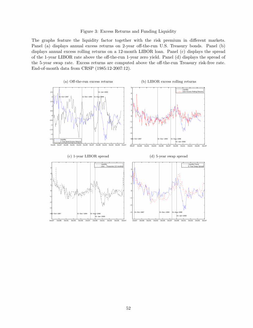
We estimate the model and obtain a measure of funding liquidity value from a sample of end-of-month bond prices running from December 1985 until the end of 2007.7 Hence, our results cannotbe attributed to the extreme influence of 2008. In a concluding section, we repeat the estimationincluding 2008 and find that the importance of funding liquidity increases. Our empirical findingscan be summarized as follows. Panel (a) of Figure 2 presents the measure of funding liquidity value.Clearly, it exhibits significant variations through normal and crisis periods. In particular, the stockcrash of 1987, the Mexican Peso devaluation of December 1994, the LTCM failure of 1998 and therecent liquidity crisis are associated with peaks in investors’ valuation of the funding liquidity ofon-the-run bonds. The relationship with the risk premium of government bonds is illustrated inFigure 3. Panel (a) compares the funding liquidity factor with annual excess returns on a 2-yearto maturity off-the-run bond. Clearly, an increase in the value of liquidity predicts lower expectedexcess returns and, thus, higher current bond prices. For that maturity, a one-standard deviationshock to liquidity predicts a decrease in excess returns of 85 basis points [bps] compared to an

5This model captures parsimoniously the usual level, slope and curvature factors, while delivering good in-samplefit and forecasting power. Moreover, the smooth shape of Nelson-Siegel curves identifies small deviations, relative toan idealized curve, which may be caused by variations in market liquidity.

6See Longstaff (2000) for evidence that liquidity is priced for short-term U.S. Treasury security and Longstaff(2004) for U.S. Treasury bonds of longer maturities. See Collin-Dufresne et al. (2001), Longstaff et al. (2005),Ericsson and Renault (2006), Nashikkar and Subrahmanyam (2006) for corporate bonds.

7A significant tax premium cannot be disentangled from the on-the-run premium using bond ages in the earlierperiod. See Section B.

3

average excess returns of 69 bps. We obtain similar results using different maturities or investmenthorizons. Intuitively, while an off-the-run bond may be less liquid relative to an on-the-run bondwith similar characteristics, it is still viewed as a liquid substitute. In particular, it can still bequickly converted into cash, at low cost, via the funding market.

Next, we consider the predictive power of funding liquidity for the risk premium on short-term Eurodollar loans. Panel (b) of Figure 3 shows that variations of LIBOR excess returns arepositively linked to variations of funding liquidity. The relationship is significant, both statisticallyand economically. Consider excess returns from borrowing at the risk-free rate for 12 monthsand rolling a 3-month LIBOR loans. On average, returns from this strategy are not statisticallydifferent from zero since the higher term premium on the borrowing leg compensates for the 3-month LIBOR spread earned on the lending leg. However, following a one-standard deviationshock to the funding liquidity factor, rolling excess returns increase by 42 bps. We reach similarconclusions using LIBOR spreads as ex-ante measures of risk premium. The effect of fundingliquidity also extends to swap markets. Panel (d) compares the liquidity factor with the spread,above the par Treasury yield, of a swap contract with 5 years to maturity. We find that a shockto funding liquidity predicts an increase of 6 bps the 5-year swap spread. This is economicallysignificant given the higher sensitivity (i.e. duration) of this contract value to changes in yields. Ineach regression, we control for variations in the level and shape of the term structure of Treasuryyields. The marginal contribution of liquidity to the predictive power is high.

Finally, we consider a sample of corporate bond spreads from the National Association ofInsurance Commissioners (NAIC). We find that the impact of liquidity is significant and follows aflight-to-quality pattern across ratings. For bonds of the highest credit quality, spreads decrease,on average, following a shock to the funding liquidity factor. In contrast, spreads of bonds withlower ratings increase. We also compute excess returns on AAA, AA, A, BBB and High YieldMerrill Lynch corporate bond indices (see Figure 4) and reach similar conclusions. Bonds withhigh credit ratings were perceived to be liquid substitutes to government securities and offeredlower risk premium following increases of the liquidity factor. This corresponds to an average effectthrough our sample, the recent events suggests that this is not always the case.

A few empirical papers document the effects of intermediation constraints on risk premium inspecific markets8 but we differ in significant ways from existing work. First, we measure the effectof intermediation constraints directly from observed prices rather than quantities. Prices aggregateinformation about and anticipations of intermediaries wealth, their portfolios and the marginsthey face. Prices also aggregate information about other aspects of liquidity such as the level andvariability of market depth and transaction costs. Second, we also differ by studying a cross-sectionof money-market and fixed-income securities, providing evidence that funding constraints shouldbe thought as an aggregate risk factor driving liquidity premia across markets.

8See Froot and O’Connell (2008) for catastrophe insurance, Gabaix et al. (2009) for mortgage-backed securities,Garleanu et al. (2009) for index options, Adrian et al. (2009) for exchange rates and Hameed et al. (2008) for equities.

4

We introduce a measure of funding liquidity value based on the higher valuation of on-the-runbonds relative to off-the-run bonds .9 The on-the-run liquidity premium was first documented byWarga (1992). Amihud and Mendelson (1991) and, more recently, Goldreich et al. (2005) confirmthe link between the premium and expected transaction costs. Duffie (1996) provides a theoreticalchannel between on-the-run premia and lower financing costs on the repo market. Vayanos andWeill (2006) extend this view and model search frictions in both the repo and the cash marketsexplicitly.10 The key frictions differentiating bonds with identical cash flows lies in their segmentedfunding markets. The link between the repo market and the on-the-run premium has been confirmedempirically. (See Jordan and Jordan (1997), Krishnamurthy (2002), Buraschi and Menini (2002)and Cheria et al. (2004).)

We differ from the modern term structure literature in two significant ways. First, the latterfocuses almost exclusively on bootstrapped zero-coupon yields11. This approach is convenientbecause a large family of models delivers zero-coupon yields which are linear in the state variables(see Dai and Singleton (2000)). However, we argue that pre-processing the data wipes out themost accessible evidence on liquidity, that is the on-the-run premium. Therefore, we use couponbond prices directly. However, the state space is no longer linear and we handle non-linearitieswith the Unscented Kalman Filter [UKF], an extension of the Kalman Filter for non-linear state-space systems (Julier et al. (1995) and Julier and Uhlmann (1996)). We first estimate a modelwithout liquidity and, notwithstanding differences in data and filtering methodologies, our resultsare consistent with CDR. However, pricing errors in this standard term structure model revealssystematic differences within pairs, correlated with ages. Estimation of the model with liquidityproduces a persistent factor capturing differences between prices of recently issued bonds and pricesof older bonds. The on-the-run premium increases with maturity but decays with the age of a bond.These new features complete our contributions to the modeling of the term structure of interestrates in the presence of a liquidity factor.

We also differ from the recent literature using a reduced-form approach that model a convenienceyield in interest rate markets (Duffie and Singleton (1997)). A one-factor model of the convenienceyield cannot match the pattern of on-the-run premia across maturities. Moreover, the link betweenthe premium and the age of a bond cannot be captured in a frictionless arbitrage-free model. Still,Grinblatt (2001) argues that the convenience yields of U.S. Treasury bills can explain the U.S. Dollarswap spread. Recently, Liu et al. (2006) and Fedlhutter and Lando (2007) evaluate the relativeimportance of credit and liquidity risks in swap spreads. Other empirical investigations are related

9The U.S Treasury recognizes and takes advantages of this price differential: “In addition, although it is not aprimary reason for conducting buy-backs, we may be able to reduce the government’s interest expense by purchasingolder, “off-the-run” debt and replacing it with lower-yield “on-the-run” debt.” [Treasury Assistant Secretary forfinancial markets Lewis A. Sachs, Testimony before the House Committee on Ways and Means].

10Kiyotaki and Wright (1989) introduced search frictions in monetary theory and Shi (2005) extends this frameworkto include bonds. See Shi (2006) for a review. Search frictions offer a rationalization of the on-the-run premium andof the spreads between bid and ask prices quoted by market intermediaries. See Duffie et al. (2005) and the discussiontherein.).

11The CRSP data set of zero-coupon yields is the most commonly used. It is based on the bootstrap method ofFama and Bliss (1987) [FB].

5

to our work. Jump risk (Tauchen and Zhou (2006)) or the debt-gdp ratio (Krishnamurthy andVissing-Jorgensen (2007)) have been proposed to explain the non-default component of corporatespreads. Finally, Pastor and Stambaugh (2003) and Amihud (2002) provide evidence of a liquidityrisk factor in expected stock returns.

The link between interest rates and aggregate liquidity is supported elsewhere in the theoreticalliterature. Svensson (1985) uses a cash-in-advance constraint in a monetary economy. Bansal andColeman (1996) allow government bonds to back checkable accounts and reduced transaction costsin a monetary economy. Luttmer (1996) investigates asset pricing in economies with frictions andshows that with transaction costs (bid-ask spreads) there is in general little evidence against theconsumption-based power utility model with low risk-aversion parameters. Holmstrom and Tirole(1998) introduce a link between the liquidity demand of financially constrained firms and assetprices. Acharya and Pedersen (2005) propose a liquidity-adjusted CAPM model where transactioncosts are time-varying. Alternatively, Vayanos (2004) takes transactions costs as fixed but intro-duces the risk of having to liquidate a portfolio. Lagos (2006) extends the search friction argumentto multiple assets: in a decentralized exchange, agents with uncertain future hedging demand preferassets with lower search costs.

The rest of the paper is organized as follows. The next section presents the model and section IIdescribes the data. Note that the state-space representation of the model, the filtering methodand the construction of the likelihood are presented in the Appendices. We report estimationresults for models with and without liquidity in Section III. Section IV evaluates the informationcontent of liquidity for excess returns and interest rate spreads while Section V identifies economicdeterminants of liquidity. Section VII concludes.

I A Term Structure Model With Liquidity

We base our model on the Arbitrage-Free Extended Nelson-Siegel [AFENS] model introduced inCDR to which we add a liquidity factor that varies with the age and maturity of a bond. Thisextension is consistent with the absence of arbitrage in an economy with frictions (Luttmer (1996)).Finally, we contrast our approach with existing models that allow for liquidity through the specifi-cation of an unobserved convenience yield.

A Term Structure Model

The term structure model of CDR belongs to the affine family (Duffie and Kan (1996)). Allthe information relevant for the evolution of interest rates is summarized by 3 latent variables, Fi,t,and the resulting zero-coupon yield curve is given by

y(Ft,m) = a(m) + F1,tb1(m) + F2,tb2(m) + F3,tb3(m), (1)

with loadings, bi(m), given in Figure 1. Details of the model are provided in Appendix A. Inparticular, these loadings are the same as in the static Nelson-Siegel representation of forward rates

6

(Nelson and Siegel (1987), NS hereafter) and this follows directly from the model assumptions.Clearly, these smooth shapes lead to the usual interpretations of factors in terms of level, slope andcurvature.

Furthermore, the NS representation is parsimonious and robust to over-fitting. It deliversperformance in line with, or better than, other methods for pricing out-of-sample bonds in the cross-section of maturities.12 Conversely, its smooth shape is useful to identify deviations of observedyields from an idealized curve. In particular, this representation cannot fit on-the-run and off-the-run bonds simultaneously.

A dynamic extension of the NS model, the Extended Nelson-Siegel model [ENS], was firstproposed by Diebold and Li (2006) and Diebold et al. (2006). Diebold and Li (2006) documentlarge improvements in long-horizon interest rate forecasting. They argue that the ENS modelperforms better than the best essentially affine model of Duffee (2002) and point toward the model’sparsimony to explain its successes. A persistent concern, though, was that the ENS model does notenforce the absence of arbitrage. This is precisely the contribution of CDR. They derive the class ofcontinuous-time arbitrage-free affine dynamic term structure models with loadings that correspondto the NS representation. Intuitively, an AFENS model corresponds to a canonical affine model inDai and Singleton (2000) where the loading shapes have been restricted through over-identifyingassumptions on the parameters governing the risk-neutral dynamics of latent factors. For ourpurposes, imposing the absence of arbitrage restricts the model from fitting price differences thatare matched by differences in cash flows. Finally, CDR compare the ENS and AFENS models andshow that implementing these restrictions improves forecasting performances further.

B Coupon Bonds

Term structure models are usually not estimated from observed prices. Rather, coupon bondprices are converted to forward rates using the bootstrap method. This is convenient since affineterm structure models deliver forward rates that are linear in state variables. Is is also thought tobe innocuous because bootstrapped forward rates achieve near-exact pricing of the original sampleof bonds. Unfortunately, this extreme fit means that a naive application of the bootstrap pushesany liquidity effects and other price idiosyncracies into forward rates. Fama and Bliss (1987)handle this sensitivity to over-fitting by excluding bonds with “large” price differences relative totheir neighbors.13 This approach is certainly justified for many of the questions addressed in theliterature, but it removes any evidence of large liquidity effects. Moreover, the FB data set focuses

12See Bliss (1997) and Anderson et al. (1996) for an evaluation of yield curve estimation methods.13The CRSP data set of zero coupon yields is based on the approach proposed by Fama and Bliss. See also the

CRSP documentation for a description of this procedure. Briefly, a first filter includes a quote if its yield to maturityfalls within a range of 20 basis points from one of the moving averages on the 3 longer or the 3 shorter maturityinstruments or if its yield to maturity falls between the two moving averages. When computing averages, precedenceis given to bills when available and this is explicitly designed to exclude the impact of liquidity on notes and bondswith maturity of less than one year. Amihud and Mendelson (1991) document that yield differences between notesand adjacent bills is 43 basis point on average, a figure much larger than the 20 basis point cutoff. The second filterexcludes observations that cause reversals of 20 basis points in the bootstrapped discount yield function. The impactof these filters has not been studied in the literature.

7

on discount bond prices at annual maturity intervals. This smooths away evidence of small liquidityeffects remaining in the data and passed through to forward rates. These effects would be apparentfrom reversals in the forward rate function at short maturity interval. Consider three quotes forbonds with successive maturities M1 < M2 < M3. A relatively expensive quote at maturity M2

induces a relatively small forward rate from M1 to M2. However, the following normal quote withmaturity M3 requires a relatively large forward rate from M2 to M3. This is needed to compensatethe previous low rate and to achieve exact pricing as required by the bootstrap. However, thereversal cancels itself as we sum intra-period forward rates to compute annual rates.

Instead of using smoothed data, we proceed from observed coupon bonds with maturity, say,M and with coupons at maturities m = m1, . . . ,M . The price, Dt(m), of a discount bond withmaturity m, used to price intermediate payoffs, is given by

Dt(m) = exp(−m(a(m) + b(m)T Ft)

)m ≥ 0,

which follows directly from equation (8) but where we use vector notation for factors Ft and factorloadings b(m). In a frictionless economy, the absence of arbitrage implies that the price of a couponbond equals the sum of discounted coupons and principal. That is, the frictionless price is

P ∗(Ft, Zt) =M∑

m=m1

Dt(m)× Ct(m), (2)

where Zt includes (deterministic) characteristics relevant for pricing a bond. In this case, it includesthe maturity M and the schedule of future coupons and principal payments, Ct(m).

C Coupon Bonds In An Economy With Frictions

With a short-sale constraint on government bonds and a collateral constraint in the repo market,Luttmer (1996) shows that the set of stochastic discount factors consistent with the absence ofarbitrage satisfies P ≥ P ∗. These constraints match the institutional features of the Treasurymarket. An investor cannot issue new bonds to establish a short position. Instead, she mustborrow the bond on the repo market through a collateralized loan. Then, we model the price,P (Ft, Lt, Zt), of any coupon bond with characteristics Zt as the sum of discounted coupons towhich we add a liquidity term,

P (Ft, Lt, Zn,t) =Mn∑

m=1

Dt(m)× Cn,t(m) + ζ(Lt, Zn,t).

Here Zt also includes the age of the bond so that the premium varies across old and new bonds.Note that the liquidity term should be positive to be consistent with Luttmer (1996).

Theoretically, Vayanos and Weill (2006) highlights the mechanisms linking the on-the-run pre-mium to the short-sale constraint on government bonds and the collateral constraint in the repomarket (see also Duffie (1996)). They show that the combination of these constraints with search

8

frictions on the repo market induces differences in funding costs that favor recently issued bonds.Intuitively, the repo market provides the required heterogeneity between assets with identical pay-offs. An investor cannot choose which bond to deliver to unwind a repo position; she must find anddeliver the same security she had originally borrowed. Because of search frictions, then, investorsare better off in the aggregate if they coordinate around one security to reduce search costs. Inpractice, the repo rate is lower for this special issue to provide an incentive for bond holders tobring their bonds to the repo market. Typically, recently issued bonds benefit from these lowerfinancing costs, leading to the on-the-run premium. Moreover, these bonds offer lower transactioncosts adding to the wedge between asset prices (Amihud and Mendelson (1986)). Empirically, bothchannels seem to be at work although the effect of lower transaction costs appears weaker than theeffect of lower funding rates.14

Grouping observations together, and adding an error term, we obtain our measurement equation

P (Ft, Lt, Zt) = CtDt + ζ(Lt, Zt) + Ωνt, (3)

where Ct is the (N ×Mmax) payoffs matrix obtained from stacking the N row vectors of individualbond payoffs and Mmax is the longest maturity group in the sample.15 Similarly, ζ(Lt, Zt) is aN × 1 vector obtained by staking the individual liquidity premium. Dt is a (Mmax × 1) vector ofdiscount bond prices and the measurement error, νt, is a (N ×1) gaussian white noise uncorrelatedwith innovations in state variables. The matrix Ω is assumed diagonal and its elements are a linearfunction of maturity,

ωn = ω0 + ω1Mn,

which reduces substantially the dimension of the estimation problem. However, leaving the diagonalelements of Ω unrestricted does not affect our results16.

D The Liquidity Premium

The liquidity premium applies to all bonds, old and new. Our specification is based on a latentfactor which drives the common dynamics but with loadings varying with the maturity and age ofeach bond. The liquidity premium is given by

ζ(Lt, Zn,t) = Lt × βMn exp(−1

κagen,t

)(4)

14Amihud and Mendelson (1991) and Goldreich et al. (2005) consider transaction costs. Jordan and Jordan (1997),Krishnamurthy (2002) and Cheria et al. (2004) consider funding costs. See also, Buraschi and Menini (2002) for theGerman bonds market.

15Shorter payoff vectors are completed with zeros.16This may be due to the fact that the level factor explains most of yield variability. Its impact on bond prices is

linear in duration and duration is approximately linear in maturity, at least for maturities up to 10 years. Bid-askspreads increase with maturity and may also contribute to an increase in measurement errors with maturity.

9

where aget is the age, in years, of the bond at time t. The parameter βM controls the averageon-the-run premium at each fixed maturity M . Warga (1992) documents the impact of age andmaturity on the average premium. We estimate β for a fixed set of maturities and the shape of β isunrestricted between these maturities.17 Next, the parameter κ controls the on-the-run premium’sdecay with age. The gradual decay of the premium with age has been documented by Goldreichet al. (2005). For instance, immediately following its issuance (i.e.: age = 0), the loading on theliquidity factor is βM × 1. Taking κ = 0.5, the loading decreases by half within any maturitygroup after a little more than 4 months following issuance : ζ(Lt, 4) ≈ 1

2ζ(Lt, 0)). While thespecification above reflects our priors about the impact of age and maturity, the scale parametersare left unrestricted at estimation and we allow for a continuum of shapes for the decay of liquidity.However, we fix β10 = 1 to identify the level of the liquidity factor with the average premium of ajust-issued 10-year bond relative to a very old bond with the same maturity and coupons.

Equation (3) shows that omitting the liquidity term will push the impact of liquidity intopricing errors, possibly leading to biased estimators and large filtering errors. Alternatively, addinga liquidity term amounts to filtering a latent factor present in pricing errors. However, Equation (3)shows that this factor captures that part of pricing errors correlated with bond ages. Our maintainedhypothesis is that any such positive factor can be interpreted as a liquidity effect. Clearly, theimpact of age on the price of a bond can hardly be rationalized in a frictionless economy.

Intuitively, our specification delivers a discount rate function (i.e. SDF) consistent with off-the-run valuation but remains silent on the linkage with the equilibrium stochastic discount factor.Instead, we capture the impact of trading and funding frictions through the positive liquidity term.Note that a more structural specification of the liquidity premium raises important challenges. Inparticular, the on-the-run premium is a real arbitrage opportunity unless we explicitly consider thecosts of shorting the more expensive bond or, alternatively, the benefits accruing to the bondholderfrom lower repo rates and search frictions. Moreover, a joint model of the term structure of reporates and of government yields may still not be free of arbitrage unless we also model the convenienceyield of holding short-term government securities. This follows from the observation that a Treasurybill typically offers a lower yield than a repo contract with the same maturity.18

Notwithstanding these modeling challenges, theory suggests that using repo rates may improvethe identification of our premium. Unfortunately, this would restrict our analysis to a much shortersample. More importantly, it is unclear how differences in repo rates translate into differencesin yields and how other aspects of liquidity affect the on-the-run premium. Furthermore, generalcollateral and special repo rates are only available for a limited term, typically shorter than theperiod of time for which the current on-the-run bond is expected to remain special. Our strategybypasses these challenging considerations, which are beyond the scope of this paper, but stilluncovers the key element of funding liquidity.

17However, we impose that β0 = 0.18These features are absent from the current crop of term structure models with the notable exception of Cheria

et al. (2004) who allow for a convenience yield, due to lower repo rates accruing to holders of an on-the-run issue.

10

II Data

We use end-of-month prices of U.S. Treasury securities from the CRSP data set. Our sample coversthe period from January 1986 to December 2008. However, we estimate the model both with andwithout 2008 data. Before 1986, interest income had a favorable tax treatment compared to capitalgains and investors favored high-coupon bonds. The resulting tax premium and the on-the-runpremium cannot be disentangled using bond ages in the earlier period. In that period, interestrates rose steadily and recently issued bonds had relatively high coupons. Then, these recent issueswere priced at a premium both for their liquidity and for their tax benefits. Green and Ødegaard(1997) document that the high-coupon tax premium mostly disappeared when the asymmetrictreatment of interest income and capital gains was eliminated following the 1986 tax reform.

The CRSP data set19 provides quotes on all outstanding U.S. Treasury securities. We filterunreliable observations and construct bins around maturities of 3, 6, 9, 12, 18, 24, 36, 48, 60,84 and 120 months.20 Then, at each date, and for each bin, we choose a pair of securities toidentify the on-the-run premium. First, we want to pick the on-the-run security if any is available.Unfortunately, on-the-run bonds are not directly identified in the CRSP database. Instead, we usetime since issuance as a proxy and pick the most recently issued security in each maturity bin.Second, we choose the security that most closely matches the bin’s maturity. Note that pinningoff-the-run securities at fixed maturities ensures a stable coverage of the term structure of interestrates. Also, by construction, securities within each pair have the same credit quality and very closetimes to maturity. We do not match coupon rates but coupon differences within pairs are low inpractice.

The most important aspect of our sample is that whenever a security trades at a premiumrelative to its pair companion, any large price difference cannot be rationalized from small couponor maturity differences under the no-arbitrage restriction. On the other hand, price differencescommon across maturities and correlated with age will be attributed to liquidity. Note that themost recent issue for a given bin and date is not always an on-the-run security. This may be due tothe absence of new issuance in some maturity bins throughout the whole sample (e.g. 18 months tomaturity) or within some sub-periods (e.g. 84 months to maturity). Alternatively, the on-the-runbond may be a few months old, due to the quarterly issuance pattern observed in some maturitycategories. In any case, this introduces variability in age differences which, in turn, identifies howthe liquidity premium varies with age.

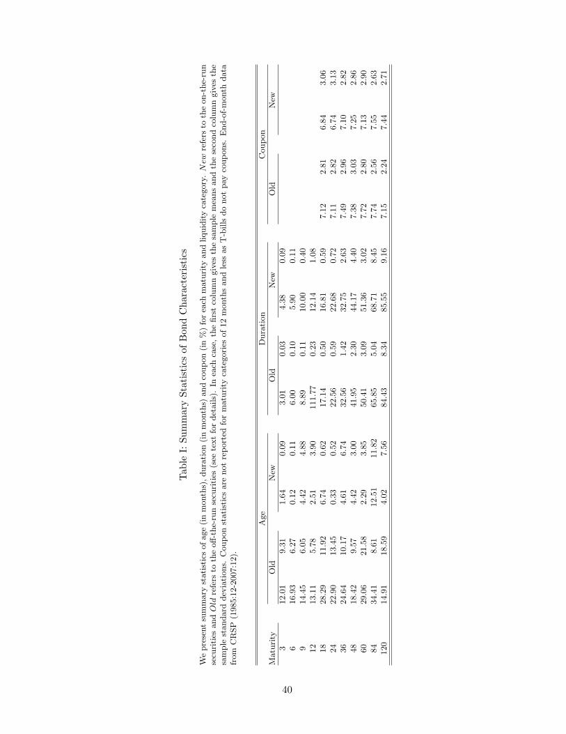
We now investigate some features of our sample of 265× 22 = 5830 observations. The first twocolumns of Table I present means and standard deviations of age for each liquidity-maturity cate-gory. The average off-the-run security is always older than the corresponding on-the-run security.Typically, the off-the-run security has been in circulation for more than a year. In contrast, theon-the-run security is typically a few months old and only a few weeks old in the 6 and 24-month

19See Elton and Green (1998) and Piazzesi (2005) for discussion of the CRSP data set.20See Apppendix B for more details on data filter.

11

categories. A relatively low average age for the recent issues indicates a regular issuance pattern.On the other hand, the relatively high standard deviations in the 36 and 84-month categories reflectthe decision by the U.S. Treasury to stop the issuance cycles at these maturities.

[Table I about here.]

Next, Table I presents means and standard deviations of duration21. Average duration is almostlinear in maturity. As expected, duration is similar within pairs implying that averages of cashflow maturities are very close. Finally, the last columns of Table I show that the term structureof coupons is upward sloping on average and the high standard deviations indicate importantvariations across the sample. This is in part due to the general decline of interest rates. Nonetheless,coupon rate differences within pairs are small on average. To summarize our strategy, differencesin duration and coupon rates are kept small within each pair but differences of ages are highlightedso that we can identify any effect of liquidity on prices that is linked to age.

III Estimation Results

Estimation is conducted via Quasi-Maximum Likelihood (QML) combined with a nonlinear filteringtechnique.22 We first estimate a restricted version of our model, excluding liquidity. Filtered factorsand parameter estimates are consistent with results obtained by CDR from zero-coupon bonds.More interestingly, the on-the-run premium reveals itself in the residuals from the benchmarkmodel. This provides a direct justification for linking the premium with the age and maturity ofeach bond. We then estimate the unrestricted liquidity model. The null of no liquidity is easilyrejected and the liquidity factor captures systematic differences between on-the-run and off-the-runbonds. Finally, estimates imply that the on-the-run premium increases with maturity but decreaseswith the age of a bond.

A Results For The Benchmark Model Without Liquidity

Estimation of the benchmark model puts the curvature parameter at λ = 0.6786, when timeperiods are measured in years. This estimate pins the maximum curvature loading at a maturityclose to 30 months. For standard errors, we reports two figures, a robust one using both the Hessiancovariance matrix and the outerproduct of the scores, which we call QML, and a second one basedon the outerproduct of the scores only, which we call OP (see details in the Appendix). Thefirst measure probably overestimates the variability23, while the second one surely underestimatesit. Therefore we decided to report both. For λ, the QML and OP standard errors are 0.0305and 0.0044, respectively. Therefore, we estimate the parameter with a lot of precision with bothmetrics.

21Duration is the relevant measure to compare maturities of bonds with different coupons.22A detailed discussion of the state-space representation and of the likelihood function is provided in Appendix C.

Non-linear filtering is based on the Unscented Kalman Filter, which is discussed in detail in Appendix D.23The Hessian is not available in closed-form and a numerical approximation for the second derivative of the entire

likelihood introduces errors.

12

[Table II about here.]

Figure 2 displays the time series of the liquidity (Panel (a)) and the term structure (Panel (b))factors. Estimates for the transition equation are given in Table IIa. The results imply averageshort and long term discount rates of 3.73% and 5.45%, respectively. The level factor is verypersistent, perhaps a unit root. This standard result in part reflects the gradual decline of interestrates in our sample. The slope factor is slightly less persistent and exhibits the usual associationwith business cycles. Its sign changes before the recessions of 1990 and 2001. The slope of the termstructure is also inverted starting in 2006, during the so-called “conundrum” episode. Finally, thecurvature factor is closely related to the slope factor.

Standard deviations of pricing errors are given by

σ(Mn) = 0.0229 + 0.0284×Mn,

(0.017, 0.0012) (0.021, 0.0006)

with QML and OP standard errors for each parameter. This implies standard deviations of %0.05and $0.31 dollars for maturities of 1 and 10 years, respectively. Using durations of 1 and 7 years,this translates into yield errors of 5.1 and 4.4 bps. Table IIIa gives more information on the fit ofthe benchmark model. Root Mean Squared Errors (RMSE) increase from $0.047 and $0.046 for3-month on-the-run and off-the-run securities, respectively, to $0.35 and $0.39 at 10-year maturity.As discussed above, the monotonous increase of RMSE with maturity reflects the higher sensitivityof longer maturity bonds to interest rates. It may also be due to higher uncertainty surroundingthe true prices, as signaled by wider bid-ask spreads. In addition, for most maturities, the RMSEis larger for on-the-run bonds. For the entire sample, the RMSE is $0.188.

Notwithstanding differences between estimation approaches, our results are consistent withCDR. Estimating using coupon bonds or using bootstrapped data provides similar pictures of theunderlying term structure of interest rates. Also, the approximation introduced when dealing withnonlinearities is innocuous. However, preliminary estimation of forward rate curves smooths awayany effect of liquidity. In contrast, our sample comprises on-the-run and off-the-run bonds. Anysystematic price differences not due to cash flow differences will be revealed in the pricing errors.

[Table III about here.]

Table IIIa confirms that Mean Pricing Errors (MPE) are systematically higher for on-the-run securities. On-the-run residuals are systematically higher than off-the-run residuals. For arecent 12-month T-Bill, the average difference is close to $0.08, controlling for cash-flow differences.Similarly, a recently issued 5-year bond is $0.25 more expensive on average than a similar but olderissue.24 To get a clearer picture of the link between age and price differences, consider Figure 6.The top panels plot residual differences within the 12-month and 48-month categories. The bottom

24Note that the price impact of liquidity increases with maturity. This is consistent with the results of Amihudand Mendelson (1991).

13

panels plot the ages of each bond in these categories. Panel (c) shows that the U.S. Treasurystopped regular issuance of the 12-month Notes in 2000. The liquidity premium was generallypositive until then but stopped when issuance ceased. Afterwards, each pair is made of old 2-yearNotes, and evidence of a premium disappears from the residuals. Panel (d) shows that there hasbeen regular issuance of 4-year bonds early in the sample. As expected, the difference betweenresiduals is generally positive whenever there is a significant age difference between the two issues.Moreover, in each case, on-the-run (i.e. low age) bonds appear overpriced compared to off-the-run(i.e. high age) bonds. This correspondence between issuance patterns and systematic pricing errorscan be observed in each maturity category. The premium increases with maturity but decreaseswith age.

Bonds with 24 months to maturity seem to carry a smaller liquidity premium than what wouldbe expected given the regular monthly issuance for this category. Note that a formal test rejectsthe null hypothesis of zero-mean residual differences. Interestingly, Jordan and Jordan (1997) couldnot find evidence of a liquidity or specialness effect at that maturity25. A smaller price premium for2-year Notes is intriguing and we can only conjecture as to its causes. Recall that the magnitudeof the premium depends on the benefits of higher liquidity, both in terms of lower transaction costsand lower repo rates. However, it also depends on the expected length of time a bond will offerthese benefits. Results in Jordan and Jordan (1997) suggests that 2-year Notes remain “special”for shorter periods of time (see Table I, p.2057). Similarly, Goldreich et al. (2005) find that theon-the-run premium on 2-year Notes goes to zero faster than other maturities, on average. This isconsistent with its short issuance cycle. Alternatively, holders of long-term bonds may re-allocatefunds from their now short maturity bonds into newly issued longer term securities. If the two-yearmark serves as a focus point for buyers and sellers, this may cause a larger volume of transactionsaround this key maturity, increasing the liquidity value of surrounding assets.

B Results For The Liquidity Model

Estimation of the unrestricted model leads to a substantial increase of the log-likelihood. Thebenchmark model is nested with 15 parameter restrictions and the improvement in likelihood issuch that the LR test-statistic leads to a p-value that is essentially zero26. The estimate for thecurvature parameter is now λ = 0.7304 with QML and OP standard errors of 0.0857 and 0.0043.Results for the transition equations are given in Table IIb. These imply average short and longterm discount rates of 4.09% and 5.76% respectively. Interestingly, the yield curve level is higheronce we account for the liquidity premium. Intuitively, the off-the-run yield curve is higher thanan otherwise unadjusted estimate would suggest. The standard deviations of measurement errors

25See Jordan and Jordan (1997) p. 2061: “With the exception of the 2-year notes [...], the average price differencesin Table II are noticeably larger when the issue examined is on special.”

26The benchmark model reached a maximum at 1998.6 while the liquidity model reached a maximum at 3482.6.

14

are given by

σ(Mn)2 = 0.0227+ 0.0251×Mn,

(0.016, 0.001) (0.0021, 0.0006)

with QML and OP standard errors for each parameter in parenthesis. Then, standard deviations are$0.048 and $0.274 for bonds with one and ten years to maturity, respectively. Using durations of 1and 7, this translates into standard deviations of 4.8 and 3.9 bps when measured in yields. Overall,parameter estimates and latent factors are relatively unchanged compared to the benchmark model.

We estimate the decay parameter at κ = 1.89 with QML and OP standard errors of 1.23and 0.45 respectively. Estimates of β are given in Table IV. Note that the level of the liquiditypremium increases with maturity.27 The pattern accords with the observations made from residualsof the model without liquidity. Moreover, Table IIIa shows that the model eliminates most of thesystematic differences between on-the-run and off-the-run bonds. There is still some evidence of asystematic difference in the 10-year category where the average error decreases from $0.31 to $0.26.We conclude that part of the variations in the 10-year on-the-run premium is not common withvariations in other maturity groups. Finally, Table IIIb shows RMSE improvements for almost allmaturities while the overall sample RMSE decreases from $0.188 to $0.151.

[Table IV about here.]

Overall, the evidence points toward a large common factor driving the liquidity premium ofon-the-run U.S. Treasury securities. We interpret this liquidity factor as a measure of the value offunding liquidity to investors. The results below show that its variations also explain a substantialshare of the risk premia observed in different interest rate markets.

IV Liquidity And Bond Risk Premia

In this section, we present evidence that variations in the value of funding liquidity, as measuredfrom a cross-section of on-the-run premia, share a common component with variations of risk premiain other interest rate markets. In other words, conditions prevailing on the funding market inducean aggregate risk factor that affects each of these markets. Of course, an increase in the liquidityfactor necessarily leads to lower excess returns for on-the-run bonds. We show here that it alsoleads to lower risk premia for off-the-run bonds as well as higher risk premia on LIBOR loans, swapcontracts and corporate bonds. Thus, although the payoffs of these assets are not directly related tothe higher liquidity of on-the-run securities, their risk premium and, hence, their price, is affectedby a common liquidity factor. To summarize, the liquidity risk in the funding market for U.S.Treasury induces a substantial price of risk in the cross-section of bond, LIBOR and swap returns.The impact across assets is similar to the often cited “flight-to-liquidity” phenomenon but remains

27The estimated average level is lower in the 10-year group relative to the 5-year and 7-year group. This is due tothe lower average age of bonds in this groups.

15

pervasive in normal market conditions. This commonality across liquidity premia accords with asubstantial theoretical literature supporting the existence of an economy-wide liquidity premium(Svensson (1985), Bansal and Coleman (1996), Holmtrom and Tirole (1998, 2001), Acharya andPedersen (2005), Vayanos (2004), Lagos (2006), Brunnermeier and Pedersen (2008), Krishnamurthyand He (2008).). The following section presents our results for various interest rate markets.28

A Off-The-Run U.S. Treasury Bonds

We first document the negative relationship between liquidity and expected excess returns onoff-the-run bonds. This is the return, over a given investment horizon, from holding a long maturitybond, in excess of the risk-free rate for that horizon. Figure 3a displays annual excess returns ona 2-year off-the-run bond along with the liquidity factor. The negative relationship is visuallyapparent throughout the sample but note the sharp variations around the crash of October 1987,the Mexican Peso crisis late in 1994, around the LTCM crisis in August 1998 and until the end ofthe millennium. At first, this tight link between on-the-run premia and returns from off-the-runTreasury bonds may be surprising. Recall that on-the-run bonds trade at a premium due to theiranticipated transaction costs and funding advantages on the cash and repo markets. However,off-the-run bonds can be readily converted into cash via the repo market. This is especially truerelative to other asset classes. In that sense, seasoned bonds are close substitutes to on-the-runbonds. Then, the risk premium of all Treasury bonds decreases in periods of high demand forthe relative funding liquidity of on-the-run bonds. Longstaff (2004) documents price differencesbetween off-the-run U.S Treasury bonds and Refcorp bonds29 with similar cash flows. He arguesthat discounts on Refcorp bond are due to “...the liquidity of Treasury bonds, especially in unsettledmarkets.”.

[Table V about here.]

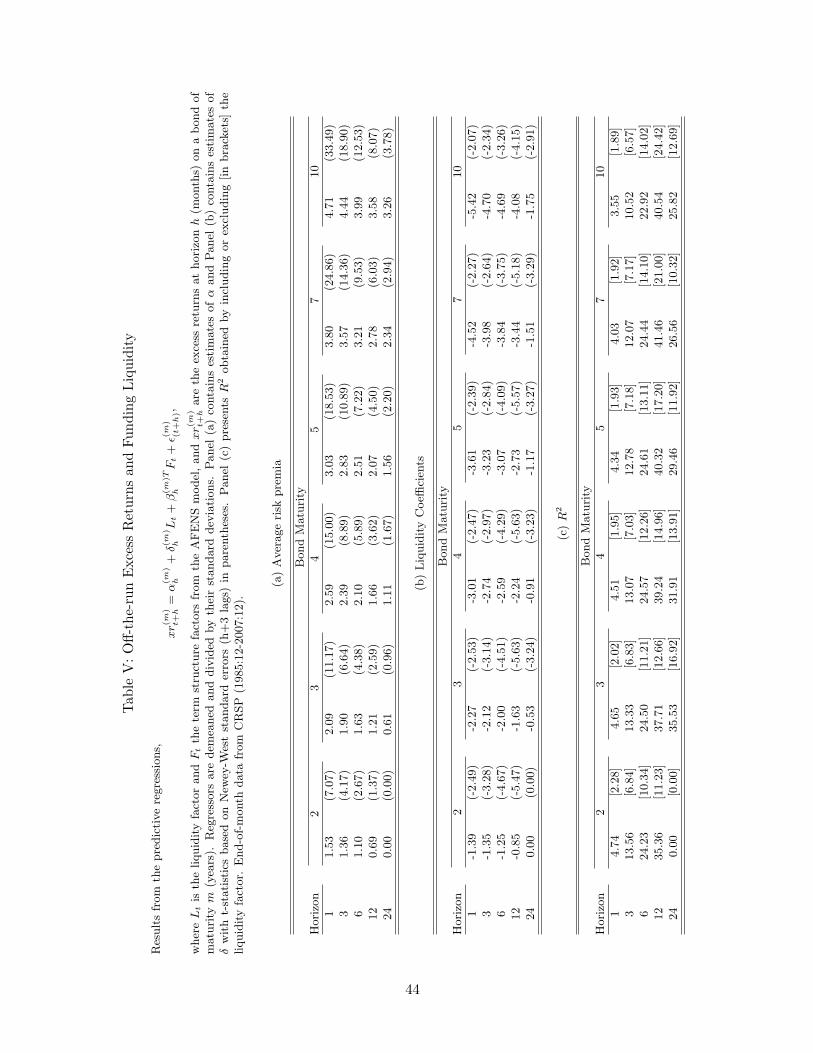
We test this hypothesis through predictive regressions of off-the-run bond excess returns onthe liquidity factor. We use the off-the-run curve from the model to compute excess returns andinclude term structure factors to control for the information content of forward rates (Fama andBliss (1987), Campbell and Shiller (1991), Cochrane and Piazzesi (2005a)). The term structurefactors spans forward rates but do not suffer from their near-collinearity. Table V presents theresults. We consider (annualized) excess returns from holding off-the-run bonds with maturities of2, 3, 4, 5, 7 and 10 years and for investment horizons of 1, 3, 6, 12, and 24 months. First, Panel (a)presents average risk premia. These range from 153 to 471 bps at one-month horizon and from 69

28All the results below are robust to choice of the off-the-run yield curve used to compute excess returns or spreads.Unless otherwise stated we use off-the-run yields computed from the model to compute excess returns. Using off-the-run zero-coupon yields from the Svensson, Nelson and Siegel method (Gurkaynak et al. (2006)) available at(http://www.federalreserve.gov/pubs/feds/2007) does not affect the results. Also, for ease of interpretation, westandardize each regressor by subtracting its mean and dividing by its standard deviation. For each risk premiumregression, the constant corresponds to an estimate of the average risk premium and the coefficient on the liquidityfactor measures the impact on expected returns, in basis points, of a one-standard deviation shock to liquidity.

29Refcorp is an agency of the U.S. government. Its liabilities have their principals backed with U.S. Treasury bondsand coupons explicitly guaranteed by the U.S. Treasury.

16

to 358 bps at annual horizon. These large excess returns are consistent with an average positiveterm structure slope and with a period of declining interest rates. Panel (b) presents estimatesof the liquidity coefficients. The results are conclusive. Estimates are negative and significant atall horizons and maturities. Moreover, the impact of liquidity on excess returns is economicallysignificant. At a one-month horizon a one-standard deviation shock to our measure of fundingliquidity lowers expected excess returns obtained from off-the-run bonds by 187 and 571 bps formaturities of two and ten years respectively. At this horizon, R2 statistics range from 7.34% to4.23% (see Panel (c)). Regressions based on excess returns at an annual horizon correspond to thecase studied by Cochrane and Piazzesi (2005a) who document the substantial predictability of USTreasury excess returns from forward rates. The impact of funding liquidity is substantial. A one-standard deviation shock decreases expected excess returns by 103 basis points at 2-year maturityand by as much as 358 basis points at 10-year maturity. At this horizon, R2 are substantially higher,ranging from 43% and 50%. Of course, these coefficients of variation pertain to the joint explanatorypower of all regressors. Panel (c) also presents, in brackets, the R2 of the same regressions butexcluding the liquidity factor. The liquidity factor accounts for more or less half of the predictivepower of the regressions.

The regressions above used excess returns and term structure factors computed from the termstructure model. One concern is that model misspecification leads to estimates of term structurefactors that do not correctly capture the information content of forward rates or that it inducesspurious correlations between excess returns and liquidity. As a robustness check against bothpossibilities, we re-examine the predictability regressions but using excess returns and forward ratesavailable from the CRSP zero-coupon yield data set. From this alternative data set, we computeannual excess returns on zero-coupon bonds with maturity from 2 to 5 years. As regressors, weinclude annual forward rates from CRSP at horizon from 1 to 5 years along with the liquidity factorfrom the model. Table VIa presents the results. Estimates of the liquidity coefficients are very closeto our previous results (see Table Vb) and highly significant. We conclude that the predictabilitypower of the liquidity factor is robust to how we compute excess returns and forward rates.

[Table VI about here.]

Furthermore, this alternative set of returns allows to check whether the AFENS model capturesimportant aspects of observed excess returns. Table VIb provides results for the regressions ofCRSP excess returns on CRSP forward rates, excluding the liquidity factor. This is a replication ofthe unconstrained regressions in Cochrane and Piazzesi (2005a) but for our shorter sample period.This exercise confirms their stylized predictability results in this sample. That is, the predictivepower of forward rates is substantial and we recover a tent-shaped pattern of coefficients acrossmaturities. Next, Table VIc provides results of a similar regressions with CRSP forward ratesbut using excess returns computed from the model. Comparing the last two panels, we see thataverage excess returns, forward rate coefficients, as well as R2s are similar across data sets. Thisis striking given that excess returns were recovered using very different approaches. The AFENSmodel captures the stylized facts of bond risk premia, which is an important measure of success for

17

term structure models.30

The evidence shows that variations of funding liquidity value induce variations in the liquiditypremium of Treasury bonds. Empirically, off-the-run US Treasury bonds are viewed as liquidsubstitutes to their recently issued counterparts and provide a hedge against fluctuations in fundingliquidity. Note that this link between conditions on the funding market and the risk premium ona Treasury bond can hardly be attributed to traditional explanations of bond risk premia such asinflation risk or interest rate risk. Instead, we argue that frictions in the financial intermediationsector affect the Treasury market. The following section considers the impact of funding liquidityon LIBOR rates.

B LIBOR Loans

In this section, we link variations of the liquidity factor with variations in the risk compensationfrom money market loans. We consider the returns obtained from rolling over a lending position inthe London inter-bank market at the LIBOR rate and funding this position at a fixed rate. Thismeasures the reward of providing liquidity in the inter-bank market. In contrast with the govern-ment bond market, higher valuation of funding liquidity predicts higher excess returns. Figure 3bhighlights the positive correlation between liquidity and rolling excess returns. Again, note thespikes in 1987, 1994, in 1998 and around the end of the millennium.

Thus, interbank loans are poor substitutes to U.S. Treasury securities in time of funding stress.The reward for providing funds in the inter-bank market is higher when the relative value of on-the-run bonds increases. Thus, the spread of a LIBOR rate above the Treasury yield reflects theopportunity costs, in terms of future liquidity, of an interbank loan compared to the liquidity ofa Treasury bonds on the repo or the cash markets. Indeed, in order to convert a loan back tocash, a bank must enter into a new bilateral contract to borrow money. The search costs of thistransaction depend on the number of willing counterparties in the market and it may be difficultat critical times to convert a LIBOR position back to cash.31

As in the previous section, we test this hypothesis formally through predictive regressions ofexcess rolling returns on the liquidity factor. As in the previous section, we consider investmenthorizons of 1, 3, 6, 12 and 24 months. However, given the short maturities of LIBOR loans weconsider the returns from rolling investments in loans with 1, 3, 6 and 12 months to maturity.Again, we use term structure factors to control for the information content of forward rates. TheLIBOR data is available from the web site of the British Bankers’ Association (BBA) and we usea sample from January 1987 to December 2007.

30Fama (1984b) originally identified this modeling challenge but see also Dai and Singleton (2002). Other stylizedfacts are documented in Fama (1976), (1984a), and(1984b), as well as Startz (1982) for maturities below 1 year. Seealso Shiller (1979), Fama and Bliss (1987), Campbell and Shiller (1991). Our conclusions hold if we use Campbelland Shiller (1991) as a benchmark. We also conclude that the empirical facts highlighted by Cochrane and Piazzesi(2005a) are not an artefact of the bootstrap method. See the discussion in Dai, Singleton, and Yang (Dai et al.) andCochrane and Piazzesi (2005b).

31Note that this does not preclude that part of the LIBOR spread is due to the higher default risk of the averageissuer compared to the U.S. government.

18

Table VII presents the results. For each loan maturity, the average excess returns is around 25bps for the shortest horizon. Returns then decrease with the horizon and become negative at thelongest horizons. This reflects the average positive slope of the term structure. In practice, fundingrolling short-term investments at a fixed rate does not produce positive returns on average.

The impact of liquidity is unambiguously positive for all horizons and maturities with t-statisticsabove 5 in most cases. Interestingly, the impact of the liquidity increases with the horizon. A one-standard deviation shock to the value of liquidity increases returns on a rolling investment in one-month LIBOR loans by 16 and 90 bps at horizons 3 and 24 months, respectively. Results are similarfor other maturities. In fact, the impact is sufficiently large that returns are positive on average,and the risk premium is higher than the slope of the term structure. This reflects the persistenceof the liquidity premium. The R2 from these regressions range from 30% to 50%. Moreover, thecontribution of the liquidity factor to the predictability of LIBOR returns is substantial, generallydoubling the R2, or more. In the case of annual excess rolling returns from 3-month loans, thepredictive power increases from 10.8% to 43.2% when we include the liquidity factor.

An alternative indicator of ex-ante returns from investment in the inter-bank market is the sim-ple spread of LIBOR rates above risk-free zero-coupon yields. As an alternative test, we computeLIBOR spreads on loans with maturities of 1, 3, 6 and 12 months and consider regressions of thesespreads on the liquidity and term structure factors. Panel (c) shows the positive relationship be-tween liquidity and the 12-month LIBOR spread. Table VIIIa presents results from the regressions.A one-standard deviation shock to liquidity is associated with concurrent increases of 16, 12, 8 and6 bps for loans with maturity of 1, 3, 6 and 12 months, respectively. Finally, one potential issue isthe use of a short-term Treasury yield in the computation of excess returns. The positive liquiditycoefficients could be due to variations of the liquidity factor that are negatively correlated withvariations in short-term zero rates. But this is not the case in practice. The impact of liquidity ispurged from these yields since we used off-the-run yields computed from the model but shutting-offthe impact of liquidity (i.e. using age = ∞). Moreover, the same results obtain if we use off-the-runyields based on Gurkaynak et al. (2006) available from the Federal Reserve Board of Governors.Finally, conditional on the term structure factors, variations of the liquidity factor have no impacton short-term off-the-run yields.32 In particular, using a projection of short-term rates on the termstructure we find that the liquidity factor has little explanatory power for the residuals.

C Swap Spreads

The impact of funding liquidity extends to the swap market. This section documents the linkbetween the liquidity factor and the spread of swap rates above Treasury yields. To the extentthat swap rates are determined by anticipations of future LIBOR rates, results from the previoussection suggest that swap spreads increase with the liquidity factor. Moreover, variations in fundingliquidity may affect the swap market directly since the same intermediaries operate in the Treasuryand the swap markets. We do not distinguish between these alternative channels here.

32Results available from the authors.

19

[Table VIII about here.]

We obtain a sample of swap rates from DataStream, starting in April 1987 and up to December2007. We focus on swaps with maturities of 2, 5, 7 and 10 years and compute their spreads abovethe yield to maturity of the corresponding off-the-run par yield. Figure 3d compares the liquidityfactor with the 5-year swap spread. The positive relationship is apparent. Next, we performregressions of swap spreads on funding liquidity. As above, we use off-the-run yields to computespreads and include the term structure factor as conditioning information. Hence the measuredimpact of funding liquidity on swap spreads cannot be attributed to the presence of short-termgovernment yields on the l.h.s.

Results are reported in Table VIIIb. First, the average spread rises with maturity, from 44 to53 bps, and extends the pattern of LIBOR risk premia. Next, estimates of the liquidity coefficientsimply that, controlling for term structure factors, a one-standard deviation shock to liquidity raisesswap spreads from 5 to 7 basis points across maturities. The estimates are significant, both staticallyand economically, given the higher price sensitivities of swap to change in yields. For a 5-year swapwith duration of 4.5, say, the price impact of a 6 basis point change is $0.27 for a notional of $100.This translates in substantial returns given the leveraged nature of swap positions.33 Finally, theexplanatory power of liquidity is high and increases with maturity.

Interestingly, funding liquidity affects swap spreads and LIBOR spreads similarly. This suggeststhat anticipations of liquidity compensation in the interbank loan market, rather than liquidity risk,is the main driver behind the aggregate liquidity component of swap risk premium. This supportsprevious literature (Grinblatt (2001), Duffie and Singleton (1997), Liu et al. (2006) and Fedlhutterand Lando (2007)) pointing toward LIBOR liquidity premium as an important driver of swapspreads. However, we show that the liquidity risk underlying a substantial part of that premium isnot specific to the LIBOR market but reflects risks faced by intermediaries in funding markets.

D Corporate Spreads

The impact of funding liquidity extends to the corporate bond market. This section measuresthe impact of the liquidity factor on the risk premium offered by corporate bonds. Empirically, wefind that the impact of liquidity has a “flight-to-quality” pattern across credit ratings. Followingan increase of the liquidity factor, excess returns decrease for the higher ratings but increase forthe lower ratings. Our results are consistent with the evidence that default risk cannot rationalizecorporate spreads. Collin-Dufresne et al. (2001) find that most of the variations of non-defaultcorporate spreads are driven by a single latent factor. We formally link this factor with fundingrisk. Our evidence is also consistent with the differential impact of liquidity across ratings found byEricsson and Renault (2006). However, while they relate bond spreads to bond-specific measuresof liquidity, we document the impact of an aggregate factor in the compensation for illiquidity.

33We do not use returns on swap investment to measure expected returns. Swap investment requires zero initialinvestment. Determining the proper capital-at-risk to use in returns computation is somewhat arbitrary. It should beclear from Figure 3d that receiving fixed, and being exposed to short-term LIBOR fluctuations, will provide greatercompensation when the liquidity premium is elevated.

20

Our analysis begins with Merrill Lynch corporate bond indices. We consider end-of-month datafrom December 1988 to December 2007 on 5 indices with credit ratings of AAA, AA, A, BBBand High Yield [HY] ratings (i.e. HY Master II index), respectively. In a complementary exercise,below, we use a sample of NAIC transaction data.34 As in earlier sections, we measure the impact ofliquidity on corporate bonds through predictive excess returns regressions. For each index, and eachmonth, we compute returns in excess of the off-the-run zero coupon yield for investment horizonsof 1, 3, 6, 12 and 24 months. We then project returns on the liquidity and term structure factors.Again, we use off-the-run yields to compute excess returns and include term structure factors tocontrol for the information content of the yield curve. The first Panel of Table IX presents theresults.

First, as expected, average excess returns are higher for lower ratings. Next, estimates of theliquidity coefficients show that the impact of a rising liquidity factor is negative for the higherratings and becomes positive for lower ratings. A one-standard deviation shock to the liquidityfactor leads to decreases in excess returns for AAA, AA and A ratings but to increases in excessreturns for BBB and HY ratings. Excess returns decrease by 1.78% for AAA index but increaseby 3.12% for the HY index. For comparison, the impact on Treasury bonds with 7 and 10 years tomaturity was -4.52% and -5.42%. Thus, on average, high quality bonds were considered substitutes,albeit imperfect, to U.S. Treasuries as a hedge against variations in funding conditions. On theother hand, lower-rated bonds were exposed to funding market shocks.

The differential impact of liquidity on excess returns across ratings suggests a flight-to-liquiditypattern. We consider an alternative sample, based on individual bond transaction data from theNAIC. While this sample covers a shorter period, from February 1996 until December 2001, the sam-ple comprises actual transaction data and provides a better coverage of the rating spectrum. Oncerestricted to end-of-month observations, the sample includes 2,171 transactions over 71 months. Topreserve parsimony, we group ratings in five categories.35 We consider regression of NAIC corporatespreads on the liquidity and term structure factors but we also include the control variables usedby Ericsson and Renault (2006). These are the VIX index, the returns on the S&P500 index, ameasure of market-wide default risk premium and an on-the-run dummy signalling whether thatparticular bond was on-the-run at the time of the transaction. Control variables also include thelevel and the slope of the term structure of interest rates.36.

The panel regressions of credit spreads for bond i at date t are given by

sprdi,t = α + β1LtI(Gi = 1) + · · ·+ β5LtI(Gi = 5) + γTh Xt + εi,t (5)

where Lt is the liquidity factor and I(Gi = j) is an indicator function equal to one if the credit34We thank Jan Ericsson for providing the NAIC transaction data and control variables. See Ericsson and Renault

(2006) for a discussion of this data set.35Group 1 includes ratings from AAA to A+, group 2 includes ratings A and A-, group 3 includes ratings BBB+,

BBB and BBB-, group 4 includes ratings CCC+, CCC and CCC- while group 5 includes the remaining ratings downto C-

36We do not include individual bond fixed-effects as our sample is small relative to the number (998) of securities.

21

rating of bond i belongs in group j = 1, . . . , 5. Control variables are grouped in the vector Xt+h.Table IXb presents the results. The flight-to-quality pattern clearly emerges from the results. Forthe highest rating category, an increase in liquidity value of one standard deviation decreases spreadsby 31 and 20 basis points in groups 1 and 2 respectively. The effect is smaller and statisticallyundistinguishable from zero for group 3. Coefficients then become positive implying increases inspreads of 25 and 26 basis points for groups 4 and 5, respectively. This is an average effect throughtime and across ratings within each group.37

The pattern of liquidity coefficients obtained from excess returns computed from Merrill Lynchindices and spreads computed from NAIC transactions differ. While results from Merrill Lynch wereinconclusive, estimates of liquidity coefficients obtained from NAIC data confirm that a shock tofunding liquidity leads to lower corporate spreads in the highest rating groups but higher corporatespreads in the lowest rating groups. Two important differences between samples may explain theresults. First, the composition of the index is different from the composition of NAIC transactiondata. The impact of liquidity on corporate spreads may not be homogenous across issues. Forexample, the maturity or the age of a bond, the industry of the issuer and security-specific optionfeatures may introduce heterogeneity. Second, Merrill Lynch indices cover a much longer time span.The pattern of liquidity premia across the quality spectrum may be time-varying.

E Discussion

Focusing on the common component of on-the-run premia filters out local or idiosyncraticdemand and supply effects on Treasury bond prices. The results above show that this measure offunding liquidity is an aggregate risk factor affecting money market instruments and fixed-incomesecurities. These assets carry a significant, time-varying and common liquidity premium. That is,when the value of the most-easily funded collateral rises relative to other securities, we observevariations in risk premia for off-the-run U.S. government bonds, eurodollar loans, swap contracts,and corporate bonds. Empirically, the impact of aggregate liquidity on asset pricing appearsstrongly during crisis and the pattern is suggestive of a flight-to-quality behavior. Nevertheless, itsimpact is pervasive even in normal times.

Note that these regressions assumed a stable relationship between risk premium and fundingliquidity. One important alternative is that the sign and the size of the impact of funding conditionsitself depend on the intensity of the funding shock, as suggested by recent experience. In particular,while corporate bonds with high ratings may be substitutes to Treasury bonds in good times,they experience large risk premium increases in funding crises. Another alternative is that therelationship between funding liquidity and risk premium experiences permanent break, or shiftsfrom one regime to another. An interesting illustration of this case is given by U.S. Agency Bonds.Figure 5 displays the funding liquidity factor against annual excess returns on an index of U.S.

37We do not report other coefficients. Briefly, the coefficient on the level factor is negative and significant. Allother coefficients are insignificant but these results are are not directly comparable with Ericsson and Renault (2006)due to differences of models and sample frequencies.

22

Agency bonds with 10 years to maturity. In the first half of the sample, up until 1998, they behavemuch like government bonds. Investors see them as substitutes and require a lower risk premiumwhen the value of funding liquidity is higher. In contrast, perhaps with the hindsight of the liquiditycrisis of the summer of 1998, Agency bonds were not considered as liquid substitutes in the secondhalf of the sample. Post-1998, the risk premium on an Agency bond rises when funding liquidity ismore valuable. We consider that these variations in the exposure to funding liquidity may explainthe weak statistical evidence for the case of corporate bonds. We leave the detailed studies of thesevariations for future research.

Jointly, the evidence is hard to reconcile with theories based on variations of default probability,inflation or interest rates and their associated risk premia. Instead, we link substantial risk premiumvariations to conditions in the funding markets. This supports the theoretical literature thatemphasizes the role of borrowing constraints faced by financial intermediaries (Gromb and Vayanos(2002), He and Krishnamurthy (2007)) and, in particular, that highlights the role of funding marketsin financial intermediation (Brunnermeier and Pedersen (2008)). Different securities serve, in part,and to varying degrees, to fulfill investors’ uncertain future needs for cash and their risk premiumdepend on the ability of intermediaries to provide immediacy in each market. In this context, itis interesting that the liquidity premium of government bonds appears to decrease when fundingliquidity becomes scarce. This confers a special status to government bonds, and possibly tohigh-quality corporate bonds, as a hedge against variations in funding liquidity. We leave forfurther research the cause of this special attribute of government bonds. The next section identifiescandidate determinants of liquidity valuation and characterizes aggregate liquidity in terms ofknown economic indicators.

V Determinants Of Liquidity Value

Funding liquidity aggregates very diverse economic information. Theory suggests that the value offunding liquidity depends on investors’ demand for immediacy on markets where intermediaries areactive. Funding costs will also vary with the capital position and the access to capital (present andfuture) of financial intermediaries that obtain leverage through secured loans. Finally, conditionsin the funding market are affected by the availability of funds and, thus, by the relative tightnessof monetary policy. In this section, we check if the funding liquidity factor is related to observableconditions in the funding markets.

Summarizing the results, we first find that the value of funding liquidity, measured by the on-the-run factor, varies with changes in monetary aggregates and in bank reserves. Second, it alsovaries with aggregate wealth and aggregate uncertainty as measured by valuation ratios and option-implied volatility of the SP500 stock index. Third, the on-the-run premium rises when recentlyissued bonds offers relatively lower bid-ask spreads. Together, the results support our interpretationof the funding liquidity factor. An important observation is that the funding liquidity factor showsno significant relationship with measures of inflation and of real activity. While these variables are

23

crucial, in the context of term structure models, for modeling interest rate dynamics, the evidencepresented here shows that funding liquidity is an important component of interest rates term premia.Moreover, the results show that the Fed affects asset prices not only through its impact on realinterest rates and inflation but, also, through its influence on funding conditions and, ultimately, onliquidity premia across markets. Finally, we found (but do not report) that the Pastor-Stambaughmeasure of liquidity risk from the stock market is unrelated to our measure of funding liquidityrisk. We conjecture that the measure of Pastor-Stambaugh differs because it relates to variationsof spot market liquidity while our liquidity factor relates to variations of funding market liquidity.

In the following, we proceed via a two-step approach. In a first set of regressions, we use themacroeconomic factors of Ludvigson and Ng (2009) that summarize 132 U.S. macroeconomic series.This approach is parsimonious and agnostic. It allows us to consider the information content froma broad set of economic indicators with no prior on their relative importance. The results fromthis first step lead us to zoom on a subset of observed macroeconomic variables, bypassing anypotential measurement errors induced in the construction of factors. This second step confirms theimportance of reserves held by commercial banks at the Fed and of the rates of growth of monetaryaggregates as determinants of funding liquidity.

A Macroeconomic Factors

Ludvigson and Ng (2009) [LN hereafter] summarize 132 US macroeconomic series into 8 princi-pal components. They then explore parsimoniously the predictive content of this large informationset for bond returns. Their main result is that that a “real” factor and an “inflation” factor38 havesubstantial predictive power for bond excess returns beyond the information content of forwardrates. They also find that a “financial” factor is significant but that much of its information con-tent is subsumed in the Cochrane-Piazzesi measure of bond risk premia. For our purposes, thesefactors provide a first way to explore the information content of a broad set of macroeconomicvariables for the funding liquidity factor. We find that the funding liquidity factor is unrelatedto the “real” and “inflation” factors. Our previous results showed that funding liquidity is alsounrelated to the Cochrane-Piazzesi factors. Table X displays results from a regression of liquidityon macroeconomic factors (Regression A) from LN and confirms that the funding liquidity factorshares tight linkages with the macroeconomy.39 The explanatory power is high, with an R2 of 58%.

[Table X about here.]

First, the “financial” factor is significant. This factor relates to different interest rate spreads,which is consistent with the evidence above that the liquidity factor predicts risk premia across

38Ludvigson and Ng (2009) use univariate regressions of individual series on each principal component to charac-terize its information content. For example, the “real” factor was labeled as such because it has high explanatorypower for real quantities (e.g. Industrial Production).

39A significant link between liquidity and one of the principal components of LN does not necessarily require thatthis component predicts bond excess returns. The liquidity factor is endogenous and its loadings on the underlyingmacroeconomic variables is unlikely to be linear or constant through time.

24

markets.40 Next, the F6 and F7 factors are significant and share a similar and extremely interest-ing interpretation: these are “monetary conditions” factors. Both are linked to the rate of changein reserves and non-borrowed reserves of depository institutions. Next, factor F6 has most in-formation for the rate of change of the monetary base and the M1 measure of money stock andsome information from the PCE indices. Beyond bank reserves, factor F7 is most informative forthe spreads of commercial paper and three-month Treasury bills above the Federal Reserve fundsrate. Overall, this suggests an important channel between monetary policy and the intermediationmechanism and, ultimately, with variations in the valuation of marketwide liquidity. These resultsare consistent with Longstaff (2004), who establishes a link between variations of RefCorp spreadsand measures of flows into money market mutual funds, Longstaff et al. (2005), who document asimilar link for the non-default component of corporate spreads and, finally, Chordia et al. (2005),who document that money flows and monetary surprises affect measures of bond market liquidity.

We also find that the liquidity factor is related to the “real”, “inflation” factors (i.e. F1 andF4), which may be caused by the impact of the Fed’s actions on funding markets. But we showbelow that their significance is not robust when we combine regressors. Factor F5 is also significantbut not robust. This is a “housing activity” factor that contains information on housing starts andnew building permits. Its significance appears to be limited to the early part of the sample and isnot robust to the inclusion of bid-ask spread information.

B Transaction Costs Variables

Coupon bond quotes from the CRSP data set include bid and ask prices. At each point in time,we consider the entire cross-section of bonds and compute the difference between the median andthe minimum bid-ask spreads. This measures the difference in transaction costs between the mostliquid bond and a typical bond. Table X presents the results from a regression of liquidity on thismeasure of relative transaction costs. The coefficient is positive and significant. The liquidity factorincreases when the median bid-ask spread moves further away from the minimum spread. Thatis, on-the-run bonds become more expensive when they offer relatively lower transaction costs.The explanatory power of bid-ask information is substantial, as measured by an R2 of 37.7%.However, there is a sharp structural break in this relationship. Most of the explanatory power andall of the statistical evidence is driven by observations preceding 1990 as made clear by Figure 7a.The first break in this process coincides with the advent of the GovPX platform while the secondbreak, around 1999, matches the introduction of the eSpeed electronic trading platform. Althoughtransaction costs contribute to the on-the-run premium (see e.g. Goldreich et al. (2005)), the lackof variability since these breaks implies a lesser role in the time variations of the premium.

40LN found that the information content of the “financial” factor for excess returns is subsumed in the CP factor.Recall from Section A that the information content of the funding liquidity factor is not subsumed by the Cochrane-Piazzesi factor.

25

C Aggregate Uncertainty

The valuation of liquidity should increase with higher aggregate uncertainty. We use impliedvolatility from options on the S&P 500 stock index as proxy for aggregate uncertainty. The S&P500index comprises a large share of aggregate wealth and its implied volatility can be interpreted asa forward looking indicator of wealth volatility. The sample comprises monthly observations ofthe CBOE VOX index from January 1986 until the end of 2007. Table X presents results from aregression of liquidity on aggregate uncertainty (Regression C). The R2 is 7.9% and the coefficientis significantly positive. A one-standard deviation shock to implied volatility raises the liquidityfactor by 0.052. Figure 7b shows the measures of volatility and funding liquidity until the end of2008. Clearly, peaks in volatility are associated with rises in liquidity valuation. The evidence ismitigated by the period around 2002 where very low funding liquidity value was not matched witha proportional decrease of implied volatility.

D Combining Regressors

Finally, Table Xa reports the results from a regression combining all the economic informa-tion considered above (Regression D). The coefficient on the relative bid-ask spread decreases butremains significant. On the other hand, the coefficient on the VXO changes sign and becomes in-significant. The information from the VXO measure is subsumed in other regressors. In particular,VXO is positively correlated with the stock market factor (i.e. F8) and this factor’s coefficient dou-bles. Finally, among the macro factors, only the “monetary conditions” factors remain significantwhen conditioning on transaction costs and aggregate uncertainty information. Note, however, thatthese results were based on unobservable macroeconomic factors estimated. In the following section,we bypass this potential measurement error issue and provide further evidence of the relationshipbetween our funding liquidity factor and conditions in funding markets.

E Reserves And Money Aggregates

To some extent, each of the macroeconomic factors of Ludvigson and Ng (2009) mixes infor-mation from all of the macroeconomic variables they consider. With the hindsight from the lastsection, we measure conditions in the market for funds directly from observable variables. Weproject the funding liquidity factor on the quantity of non-borrowed reserves held by commercialbanks at the Fed and the annual growth rates of standard monetary aggregates (i.e. M0, M1, M2).Note that these variables covers our entire sample. Moreover, we still control for transaction costsand aggregate uncertainty. Table Xb presents the results. Regression E includes bank reservesand monetary aggregate growth rates. The coefficient on bank reserves and M2 annual growth arenegative and significant. The annual growth rates of M0 and M1 are insignificant. These resultsare unchanged when we control for transaction costs and for aggregate uncertainty (see RegressionF).

Overall the evidence points toward two broad channels in the determination of the value of fund-ing liquidity. First, similar to the model of Krishnamurthy and He (2008), aggregate uncertainty

26

and aggregate wealth affect the intermediaries’ ability to provide liquidity. Second, conditions inthe market for funds, as measured by bank reserves and growth in monetary aggregates, also affectthe equilibrium value of funding liquidity.

VI The Events Of 2008

We repeat the estimation of the model including data from 2008. Figure 8 presents the liquidity(Panel 8a) and the term structure (Panel 8b) factors. The latter shows a sharp increase in the cross-section of on-the-run premium. In fact, this large shock increases the volatility of the liquidity factorsubstantially. The dramatic variations of spreads, and of the funding liquidity factor, in 2008 raisequestions as to whether a constant volatility model correctly filter the impact of liquidity on bondprices throughout the sample. With this potential issue in mind, we now report results obtainedwhen including 2008 in the estimation sample. First, looking at Figure 7b and 7a we see that thisspike was associated with a large increase in the SP500 implied volatility but, interestingly, thedifference between the minimum and median bid-ask spreads remained stable. This supports ourinterpretation that the liquidity factor finds its roots in the funding market.

Not surprisingly, including 2008 only increases the measured impact of the common fundingliquidity factor on bond risk premia. Empirically, most of the regressions above lead to higherestimates for the liquidity coefficient.41 An interesting case, though, is the behavior of corporatebond spreads. Clearly corporate bond spreads increased sharply over that period, indicating anincrease in expected returns. Figure 9 compares the liquidity factor with the spread of the AAA andBBB Merrill Lynch index. In the sample excluding 2008, the estimated average impact of a shockto funding liquidity was negative for AAA bonds and positive for BBB. The large and positivelycorrelated shock in 2008 reverses this conclusion for AAA bonds. But note that AAA spreads andthe liquidity factor were also positively correlated in 1998. This confirms our conjecture that thebehavior of high-rating bonds is not stable and depends on the nature or the size of the shock tofunding liquidity. However, this does not affect our conclusion that corporate bond liquidity premiashare a common component with other risk premia due to funding risk. Instead, it suggests thatthe relationship exhibits regimes through time.

Results about the economic determinants of liquidity are also robust to the inclusion of theyear 2008. But note that the crisis is characterized by a positive correlation between monetaryaggregates and the liquidity factor in 2008. This is in contrast with the overall sample where theavailability of funds was negatively related to the liquidity factor. However, this is due to theendogenous response of the Fed to conditions in the financial system. Clearly, had the Fed notintervened, the value of funding liquidity would have increased with reductions of funds availableto intermediaries.

41We include all tables and figures for the risk premia regressions on all markets and for the macroeconomicdeterminants of liquidity in an appendix available upon request from the authors.

27

VII Conclusion

We augment the Arbitrage Free Extended Nelson-Siegel term structure model of Christensen et al.(2007) by allowing for a liquidity factor driving the on-the-run premium. Estimation of the modelproceeds directly from coupon bond prices using a non-linear filter. We identify from a panel ofTreasury bonds a common liquidity factor driving on-the-run premia at different maturities. Itseffect increases with maturity and decreases with the age of a bond.

We interpret this factor as a measure of funding liquidity. It measures the value of the lowerfunding and transaction costs of on-the-run bonds. We find that funding liquidity predicts asubstantial share of the risk premium on off-the-run bonds. It also predicts LIBOR spreads, swapspreads and corporate bond spreads. The pattern across interest rate markets and credit ratingsis consistent with accounts of flight-to-liquidity events. However, the effect is pervasive in normaltimes. The evidence points toward the importance of the funding market for the intermediationmechanism and, hence, for asset pricing. Our results are robust to changes in the data set and tothe inclusion of term structure information.

The liquidity factor varies with transaction costs on the secondary bond market. More impor-tantly, we find that the value of liquidity is related to narrow measures monetary aggregates andmeasures of bank reserves. It also varies with measures of stock market valuations and aggregateuncertainty. The ability of intermediaries to meet the demand for immediacy depends, in part, onfunding conditions and induces a large common liquidity premium in key interest rate markets. Inparticular, our results suggest that the behavior of the Fed is a key determinant of the liquiditypremium. We leave this, as well as the potential impact of funding liquidity on stock markets, asopen research questions. In this context, the measure of funding liquidity proposed here can beused as real-time measure of liquidity premia.

28

VIII Appendix

A Arbitrage-Free Term Structure Model

This section follows Christensen et al. (2007) and provides a description of the term structuremodel. The k = 3 term structure factors are stacked in the vector Ft. Its dynamics under therisk-neutral measure Q is described by the stochastic differential equation

dFQt = KQ(θQ − Ft) + ΣdWQ

t , (6)

where dWt is a standard Brownian motion process. Combined with the assumption that the shortrate is affine in all three factors, this leads to the usual affine solution for discount bond yields. Inthis context, CDR show that if the short rate is defined as rt = F1,t +F2,t and if the mean-reversionmatrix KQ is restricted to

KQ =

0 0 00 λ −λ0 0 λ

, (7)

then the absence of arbitrage opportunity implies the discount yield function,

y(Ft,m) = a(m) + F1,tb1(m) + F2,tb2(m) + F3,tb3(m), (8)

with loadings given by

b1(m) = 1,

b2(m) =(

1− exp (−mλ)mλ

),

b3(m) =(

1− exp (−mλ)mλ

− exp (−mλ))

, (9)

where m ≥ 0 is the length of time until maturity. Finally, the constant, a(m), is given by

a(m) = −σ211

m2

6− (σ2

21 + σ222)

[1

2λ2− 1− e−mλ

mλ3+

1− e−2mλ

4mλ3

]

− (σ231 + σ2

32 + σ233)

×[

12λ2

+e−mλ

λ2− me−2mλ

4λ− 3e−2mλ

4λ2− 2(1− e−mλ)

mλ3+

5(1− e−2mλ)8mλ3

]

− (σ11σ21)[

m

2λ+

e−mλ

λ2− 1− e−mλ

mλ3

]

− (σ11σ31)[3e−mλ

λ2+

m

−2λ+

me−mλ

λ

]

− (σ21σ31 + σ22σ32)

×[

1λ2

+e−mλ

λ2− e−2mλ

λ2− 3(1− e−mλ)

mλ3+

3(1− e−2mλ)4mλ3

].

Note that the first factor has a unit root under the risk-neutral density. Then, as discussed inCDR, we have that a(m) → −∞ when m → ∞. However, this is not relevant in practice sincea(m) is relatively small for observed maturities and estimated parameter values. In particular, we

29

have that a ≈ 0 for short maturities and a(m) ≈ −1% at a maturity of 30 years. In contrast, weonly consider maturities of 10 years or less.

B Data

We use end-of-month prices of U.S. Treasury securities from the CRSP data set. We excludecallable bonds, flower bonds and other bonds with tax privileges, issues with no publicly outstandingsecurities, bonds and bills with less than 2 months to maturity and observations with either bid orask prices missing. Our sample covers the period from January 1986 to December 2008. We alsoexclude the following suspicious quotes.

CRSP ID Date#19920815.107250 August 31st 1987#19950331.203870 December 30th 1994#19980528.400000 May 30th 1998#20011130.205870 October 31th 1997#20030228.205500 February 26th 1999#20041031.202120 November 29th 2002#20070731.203870 May 31st 2006#20080531.204870 November 30th 2007

These show up as outliers in the term structure model, relative to surrounding quotes. However,including them do not affect our results. We also exclude CRSP ID #20040304.400000 sinceits maturity date precedes its issuance date, as dated by the U.S. Treasury. Finally, CRSP ID#20130815.204250 is never special and is excluded.

In 2008, the most recent 10-year issue is not always the most expensive in its maturity group.Nonetheless, the relationship between the relative valuations and ages of bonds remained stable forthe other bonds in this group. Therefore, when we extend the estimation sample to include 2008,the following bonds were selected.

Date CRSP ID#New Old

01/2008 20171115.204250 20170815.20475002/2008 20180215.203500 20171115.20425003/2008 20180215.203500 20171115.20425004/2008 20180215.203500 20171115.20425005/2008 20180515.203875 20171115.20425006/2008 20180215.203500 20171115.20425007/2008 20180215.203500 20171115.20425008/2008 20180215.203500 20170815.20475010/2008 20180215.203500 20170815.20475011/2008 20180515.203875 20170815.20475012/2008 20180515.203875 20180215.203500

C State-Space Representation And Likelihood Function

CDR show that we are free to choose the drift term, KP , in the dynamics under the physicalmeasure,

dFPt = KP (θP − Ft) + ΣdWP

t . (10)

30

Implicitly, this relies on a flexible, linear specification of the prices of risk. Intuitively, choosing aspecific set of values for the parameters of the KP matrix pins downs the parameters of the priceof risk equation. Here, we impose that KP is diagonal. In practice, the presence of the off-diagonalelements in the KP matrix does not change our results. Moreover, CDR show that allowing foran unrestricted matrix KP deteriorates out-of-sample performance. Finally, we take Σ as lowertriangular for identification purposes.

We can then cast the model within a discretized state-space representation. The state equationbecomes

(Ft − F ) = Φ(Ft−1 − F ) + Γεt, (11)

where the innovation εt is standard Gaussian, the autoregressive matrix Φ is

Φ = exp(−K

112

)(12)

and the covariance matrix Γ can computed from

Γ =∫ 1

12

0e−KsΣΣT e−Ksds. (13)

Finally, we define a new latent state variable, Lt, that will be driving the liquidity premium. Itstransition equation is

(Lt − L) = φl(Lt−1 − L) + σlεlt, (14)

where the innovation εlt is standard Gaussian and uncorrelated with εt. Then, Equations (3), (11)

and (14) can be summarized as a state-space system

(Xt − X) = ΦX(Xt−1 − X) + ΣXεt

Pt = Ψ(Xt, Ct, Zt) + Ωνt, (15)

where Xt ≡ [F Tt Lt]T and Ψ is the (non-linear) mapping of cash flows Ct, bond characteristics, Zt,

and current states, Xt, into prices, Pt.

Estimation of this system is challenging because we do not know the joint density of factors andprices. Various strategies to deal with non-linear state-space systems have been proposed in thefiltering literature: the Extended Kalman Filter (EKF), the Particle Filter (PF) and more recentlythe Unscented Kalman Filter (UKF).42 The UKF is described in greater detail in Appendix D.In practice, it delivers second-order accuracy with no increase in computing costs relative to theEKF. Moreover, analytical derivatives are not required. The UKF has been introduced in theterm structure literature by Leippold and Wu (2003) and in the foreign exchange literature byBakshi et al. (2005). Recently, Christoffersen et al. (2007) compared the EKF and the UKF for theestimation of term structure models. They conclude that the UKF improves filtering results andsubstantially reduces estimation bias.

To set up notation, we state the standard Kalman filter algorithm as applied to our model. Wethen explain how the unscented approximation helps overcome the challenge posed by a non-linearstate-space system. First, consider the case where Ψ is linear in X and where state variables and

42See Julier et al. (1995), Julier and Uhlmann (1996) and Wan and der Merwe (2001) for a textbook treatment.Another popular approach bypasses filtering altogether. It assumes that some prices are observed without errors andobtains factors by inverting the pricing equation. In our context, the choice of maturities and liquidity types thatare not affected by measurement errors is not innocuous and impacts estimates of the liquidity factor.

31

bond prices are jointly Gaussian. In this case, the Kalman recursion provides optimal estimatesof current state variables given past and current prices. The recursion works off estimates of statevariables and their associated MSE from the previous step,

Xt+1|t ≡ E [Xt+1|=t] ,

Qt+1|t ≡ E[(Xt+1|t −Xt+1)(Xt+1|t −Xt+1)T

], (16)

where =t belongs to the natural filtration generated by bond prices. The associated predicted bondprices, and MSE, are given by

Pt+1|t ≡ E [Pt+1|=t]

= Ψ(Xt+1|t, Ct+1, Zt+1), (17)

Rt+1|t ≡ E[(Pt+1|t − Pt+1)(Pt+1|t − Pt+1)T

]

= Ψ(Xt+1|t, Ct+1, Zt+1)T Qt+1|tΨ(Xt+1|t, Ct+1, Zt+1) + Ω, (18)

using the linearity of Ψ. The next step compares predicted to observed bond prices and updatestate variables and their MSE,

Xt+1|t+1 = Xt+1|t + Kt+1(Pt+1 − Pt+1|t), (19)

Qt+1|t+1 = Qt+1|t + KTt+1(Rt+1|t)−1Kt+1, (20)

where

Kt+1 ≡ E[(Xt+1|t −Xt+1)(Pt+1|t − Pt+1)T

],

= Qt+1|tΨ(Xt+1|t, Ct+1, Zt+1), (21)

measures co-movements between pricing and filtering errors. Finally, the transition equation givesus a conditional forecast of Xt+2,

Xt+2|t+1 = ΦXXt+1|t+1, (22)

Qt+2|t+1 = ΦTXQt+1|t+1ΦX + ΣXΣT

X . (23)

The recursion delivers series Pt|t−1 and Rt|t−1 for t = 1, · · · , T . Treating X1|0 as a parameter, andsetting R1|0 equal to the unconditional variance of measurement errors, the sample log-likelihoodis

L(θ) =T∑

t=1

l(Pt; θ) =T∑

t=1

[log φ(Pt+1|t, Rt+1|t)

], (24)

where φ(·, ·) is the multivariate Gaussian density.

However, because Ψ(·) is not linear, equations (17) and (18) do not correspond to the conditionalexpectation of prices and the associated MSE. Also, (21) does not correspond to the conditionalcovariance between pricing and filtering errors. Still, the updating equations (19) and (20) remainjustified as optimal linear projections. Then, we can recover the Kalman recursion provided weobtain approximations of the relevant conditional moments. This is precisely what the unscentedtransformation achieves, using a small deterministic sample from the conditional distribution offactors while maintaining a higher order approximation than linearization43. We can then use thelikelihood given in (24), but in a QML context. Using standard results, we have θ ≈ N(θ0, T

−1Ω)43See Appendix D.

32

where θ is the QML estimator of θ0 and the covariance matrix is

Ω = E[(

ζHζ−1OP ζH

)−1], (25)

where ζH and ζOP are the alternative representations of the information matrix, in the Gaussiancase. These can be consistently estimated via their sample counterparts. We have

ζH = −T−1

[∂2L(θ)∂θ∂θ′

](26)

and

ˆζOP = T−1T∑

t=1

(∂l(t, θ)

∂θ

)(∂l(t, θ)

∂θ

)T . (27)

Finally, the model implies some restrictions on the parameter space. In particular, φl and diagonalelements of Φ must lie in (−1, 1) while κ and λ must remain positive. In practice, large values ofκ or λ lead to numerical difficulties and are excluded. Finally, we maintain the second covariancecontour of state variables inside the parameter space associated with positive interest rates. Thefiltering algorithm often fails outside this parameter space. None of these constraints binds aroundthe optimum and estimates remain unchanged when the constraints are relaxed. Estimation isimplemented in MATLAB via the fmincon routine with the medium-scale (active-set) algorithm.Different starting values were used. For standard errors computations, we obtain the final Hes-sian update (BFGS formula) and each observation gradient is obtained through a centered finitedifference approximation evaluated at the optimum.

D Unscented Kalman Filter

The UKF is based on a method for calculating statistics of a random variable which undergoesa nonlinear transformation. It is based on an approximation to any non-linear transformation ofa probability distribution. It starts with a well-chosen set of points with given sample mean andcovariance. The nonlinear function is then applied to each point and moments are computed fromtransformed points. This approach has a Monte Carlo flavor but the sample is drawn accordingto a specific deterministic algorithm. It has been introduced in Julier et al. (1995) and Julier andUhlmann (1996) (see Wan and der Merwe (2001) for textbook treatment) and was first importedin finance by Leippold and Wu (2003).

Given Xt+1|t a time-t forecast of state variable for period t + 1, and its associated MSE Qt+1|tthe unscented filter selects a set of Sigma points in the distribution of Xt+1|t such that

x =∑

i

w(i)x(i) = Xt+1|t

Qx =∑

i

w(i)(x(i) − x)(x(i) − x)′ = Qt+1|t.

Julier et al. (1995) proposed the following set of Sigma points,

x(i) =

x i = 0

x +(√

Nx

1−w(0)

∑x

)(i)

i = 1, . . . ,K

x−(√

Nx

1−w(0)

∑x

)(i−K)

i = K + 1, . . . , 2K

33

with weights

w(i) =

w(0) i = 01−w(0)

2K i = 1, . . . ,K1−w(0)

2K i = K + 1, . . . , 2K

where(√

Nx

1−w(0)

∑x

)(i)

is the i -th row or column of the matrix square root. Julier and Uhlmann

(1996) use a Taylor expansion to evaluate the approximation’s accuracy. The expansion of y = g(x)around x is

y = E [g(x + ∆x)]

= g(x) + E

[D∆x(g) +

D2∆x(g)2!

+D3

∆x(g)3!

+ · · ·]

where the Di∆x(g) operator evaluates the total differential of g(·) when perturbed by ∆x, and

evaluated at x. A useful representation of this operator in our context is

Di∆x(g)i!

=1i!

n∑

j=1

∆xj∂

∂xj

i

g(x)

∣∣∣∣∣x=x

Different approximation strategies for y will differ by either the number of terms used in theexpansion or the set of perturbations ∆x. If the distribution of ∆x is symmetric, all odd-orderedterms are zero. Moreover, we can re-write the second terms as a function of the covariance matrixPxx of ∆x,

y = g(x) +(∇T Pxx∇

)g(x) + E

[D4

∆x(g)4!

+ · · ·]

Linearisation leads to the approximation ˆylin = g(x) while the unscented approximation is exactup to the third-order term and the σ-points have the correct covariance matrix by construction.In the Gaussian case, Julier and Ulhmann (1996) show that same-variable fourth moments agreeas well and that all other moments are lower than the true moments of ∆x. Then, approximationerrors of higher order terms are necessarily smaller for the UKF than for the EKF. Using a similarargument, but for approximation of the MSE, Julier and Uhlmann (1996) show that linearisationand the unscented transformation agree with the Taylor expansion up to the second-order termand that approximation errors in higher-order terms are smaller for the UKF.

34

References

Acharya, V. V. and L. Pedersen (2005). Asset pricing with liquidity risk. JFE 77.

Adrian, T., E. Etula, and H. Shin (2009). Risk appetite and exchange rates. Working Paper.

Adrian, T. and H. Shin (2008). Liquidity and leverage. Journal of Financial Intermediation,forthcoming.

Amihud, Y. (2002). Illiquidity and stock returns: cross-section and time-series effects. Journal ofFinancial Markets 5, 31–56.

Amihud, Y. and H. Mendelson (1986). Asset pricing and the bid-ask spreads. Journal of FinancialEconomics 17, 223–249.

Amihud, Y. and H. Mendelson (1991). Liquidity, maturity and the yields on U.S. treasury securities.The Journal of Finance 46, 1411–1425.

Anderson, N., F. Breedon, M. Deacon, A. Derry, and G. Murphy (1996). Estimating and interpretingthe yield curve. Series in Financial Economics and Quantitative Analysis. John Wiley & Sons.

Bakshi, G., P. Carr, and L. Wu (2005). Stochastic risk premiums, stochastic skewness in cur-rency options, and stochastic discount factors in international economies. Journal of FinancialEconomics 87.

Bansal, R. and W. Coleman (1996). A monetary explanation of the term premium, equity premiumand risk-free rate puzzle. The Journal of Political Economy 104, 396–409.

Bliss, R. (1997). Testing term structure estimation methods. Advances in Futures and OptionsResearch 9, 197–231.

Brunnermeier, M. K. and L. Pedersen (2008). Market liquidity and funding liquidity. Review ofFinancial Studies, forthcoming.

Buraschi, A. and D. Menini (2002). Liquidity risk and specialness. Journal of Financial Eco-nomics 64, 243–284.

Campbell, J. and R. Shiller (1991). Yield spreads and interest rate movements: A bird’s eye view.Review of Economic Studies 58, 495–514.

Cheria, J., E. Jacquier, and R. Jarrow (2004). A model of the convenience yields in on-the-runtreasuries. Review of Derivatives Research 7, 79–97.

Chordia, T., A. Sarkar, and A. Subrahmanyam (2005). An empirical analysis of stock and bondmarket liquidity. Review of Financial Studies 18, 85–129.

35

Christensen, J., F. Diebold, and G. Rudebusch (2007). The affine arbitrage-free class of nelson-siegelterm structure models. Technical Report 20, FRBSF.

Christoffersen, P., K. Jacobs, L. Karoui, and K. Mimouni (2007). Estimating term structure modeslusing swap rates. McGill University.

Cochrane, J. and M. Piazzesi (2005a). Bond risk premia. American Economic Review 95, 138–160.

Cochrane, J. and M. Piazzesi (2005b). Reply to Dai, Singleton and Yang.

Collin-Dufresne, P., R. Goldstein, and J. Spencer Martin (2001). The determinants of credit spreadchanges. The Journal of Finance 56, 2177–2207.

Dai, Q. and K. Singleton (2000). Specification analysis of affine term structure models. The Journalof Finance 55, 1943–1978.

Dai, Q. and K. Singleton (2002). Expectation puzzles, time-varying risk premia and affine modelof the term structure. Journal of Financial Economics 63, 415–441.

Dai, Q., K. Singleton, and W. Yang. Predictability of bond risk premia and affine term structuremodels.

Diebold, F. and C. Li (2006). Forecasting the term structure of government bond yields. Journalof Econometrics 130, 337–364.

Diebold, F., G. Rudebusch, and S. Aruoba (2006). The macroeconomy and the yield curve : Adynamic latent factor approach. Journal of Econometrics 131, 309–338.

Duffee, G. (2002). Term premia and interest rate forecast in affine model. The Journal of Fi-nance 57, 405–443.

Duffie, D. (1996). Special repo rates. The Journal of Finance 51, 493–526.

Duffie, D., N. Garleanu, and L. Pedersen (2005). Over-the-counter markets. Econometrica 73,1815–1847.

Duffie, D. and R. Kan (1996). A yield-factor model of interest rates. Mathematical Finance 6,379–406.

Duffie, D. and K. Singleton (1997). An econometric model of the term structure of interest-rateswap yields. The Journal of Finance 52, 1287–1321.

Elton, E. and T. Green (1998). Tax and liquidity effects in pricing governement bonds. The Journalof Finance 53, 1533–1562.

Ericsson, J. and O. Renault (2006). Liquidity and credit risk. The Journal of Finance 61, 2219–2250.

36

Fama, E. (1976). Forward rates as predictors of future spot rates. Journal of Financial Economics 3,361–377.

Fama, E. (1984a). The information in the term structure. Journal of Financial Economics 13,509–528.

Fama, E. (1984b). Term premium in bond returns. Journal of Financial Economics 13, 529–546.

Fama, E. and R. Bliss (1987). The information in long-maturity forward rates. American EconomicReview 77, 680–692.

Fedlhutter, P. and D. Lando (2007). Decomposing swap spreads. Working Paper.

Froot, K. and P. O’Connell (2008). On the pricing of intermediated risks: Theory and applicationto catastrophe reinsurance. Journal of Banking and Finance 32, 69–85.

Gabaix, X., A. Krishnamurthy, and O. Vigneron (2009). Limits of arbitrage: Theory and evidencefrom the mortgage-backed securities market. The Journal of Finance. Forthcoming.

Garleanu, N. and L. Pedersen (2009). Margin-based asset pricing and deviations from the law ofone price. Working Paper.

Garleanu, N., L. Pedersen, and A. Pothesman (2009). Demand-based option pricing. Review ofFinancial Studies. Forthcoming.

Goldreich, D., B. Hanke, and P. Nath (2005). The price of future liquidity : Time-varying liquidityin the U.S. treasury market. Review of Finance 9, 1–32.

Green, R. and B. Ødegaard (1997). Are there tax effects in the relative pricing of the U.S. govern-ment bonds? The Journal of Finance 52, 609–633.

Grinblatt, M. (2001). An analytic solution for interest rate swap spreads. International Review ofFinance 2, 113–149.

Gromb, D. and D. Vayanos (2002). Equilibrium and welfare in markets with financially constrainedarbitrageurs. Journal of Financial Economics 66, 361–407.

Gurkaynak, R., B. Sack, and J. Wright (2006). The u.s. treasury curve: 1961 to present. TechnicalReport 2006-28.

Hameed, A., W. Kang, and S. Vishnawathan (2008). Stock market declines and liquidity. TheJournal of Finance, forthcoming.

He, Z. and A. Krishnamurthy (2007). Intermediated asset prices. Technical report.

Holmstrom, B. and J. Tirole (1998). Private and public supply of liquidity. The Journal of PoliticalEconomy 106, 1–40.

37

Jordan, B. and S. Jordan (1997). Special repo rates: An empirical analysis. The Journal ofFinance 52, 2051–2072.

Julier, S. and J. Uhlmann (1996). A general method for approximating nonlinear transformationsof probability distributions. Robotics Research Group, University of Oxford.

Julier, S., J. Uhlmann, and H. Durrant-Whyte (1995). A new approach for filtering nonlinearsystems. The Proceedings of the American Control Conference 3, 1628–1632. Seattle.

Kiyotaki, N. and R. Wright (1989). On money as a medium of exchange. The Journal of PoliticalEconomy 97, 927–954.

Krishnamurthy, A. (2002). The bond/old-bond spread. Journal of Financial Economics 66, 463–506.

Krishnamurthy, A. and Z. He (2008). Intermediary asset prices. W14517.

Krishnamurthy, A. and J. Vissing-Jorgensen (2007). The demand for treasury debt. W12881.

Kyle, A. and W. Xiong (2001). Contagion as a wealth effect. The Journal of Finance 56, 1401–1440.

Lagos, R. (2006). Asset prices and liquidity in an exchange economy. Technical Report 373, FederalReserve Bank of Minneapolis.

Leippold, M. and L. Wu (2003). Design and estimation of multi-currency quadratic models. Euro-pean Finance Review 7, 47–73.

Liu, J., F. Longstaff, and R. Mandell (2006). The market price of risk in interest rate swaps: Theroles of default and liquidity risks. Journal of Business 79, 2337–2359.

Longstaff, F. (2000). The term structure of very short-term rates : New evidence for the expectationhypothesis. Journal of Financial Economics 58, 397–415.

Longstaff, F. (2004). The flight-to-liquidity premium in U.S. treasury bond prices. The Journal ofBusiness 77, 511–526.

Longstaff, F., S. Mithal, and E. Neis (2005). Corporate yield spreads: Default risk or liquidity?new evidence from the credit-default swap market. The Journal of Finance 60, 2213–2253.

Ludvigson, S. and S. Ng (2009). Macro factors in bond risk premia. Review of Financial Studies.forthcoming.

Luttmer, E. (1996). Asset pricing in economies with frictions. Econometrica 64, 1439–1467.

Nashikkar, A. and M. Subrahmanyam (2006). Latent liquidity and corporate bond yield spreads.Stern School of Business.

38

Nelson, C. and A. Siegel (1987). Parsimonious modeling of yield curves. The Journal of Business 60,473–489.

Pastor, L. and R. Stambaugh (2003). Liquidity risk and expected stock returns. The Journal ofPolitical Economy 111, 642–685.

Piazzesi, M. (2005). Affine term structure models. in Handbook of Financial Econometrics. Elsevier.

Shi, S. (2005). Nominal bonds and interest rates. International Economic Review 46, 579–612.

Shi, S. (2006). Viewpoint: a microfoundation of monetary economics. Canadian Journal of Eco-nomics 39, 643–688.

Shiller, R. (1979). The volatility of long-term interest rates and expectation models of the termstructure. The Journal of Political Economy 87, 1190–1219.

Shleifer, A. and R. Vishny (1997). The limits of arbitrage. The Journal of Finance 52, 35–55.

Startz, R. (1982). Do forecast errors of term premia really make a difference between long andshort rates. Journal of Financial Economics 10, 323–329.

Svensson, L. (1985). Money and asset prices in a cash-in-advance economy. The Journal of PoliticalEconomy 93, 919–944.

Tauchen, G. and H. Zhou (2006). Realized jumps on financial markets and predicting credit spreads.Technical Report 2006-35, Federal Reserve Board.

Vayanos, D. (2004). Flight to quality, flight to liquidity, and the pricing of risk. NBER (W10327).

Vayanos, D. and P.-O. Weill (2006). A search-based theory of the on-the-run phenomenon. TheJournal of Finance forthcoming.

Wan, E. and R. V. der Merwe (2001). Kalman filtering and neural network, Chapter The unscentedKalman filter. Wiley and Sons.

Warga, A. (1992). Bond returns, liquidity and missing data. The Journal of Financial and Quan-titative Analysis 27, 605–617.

39

Tab

leI:

Sum

mar

ySt

atis

tics

ofB

ond

Cha

ract

eris

tics

We

pre

sent

sum

mary

stati

stic

sofage

(in

month

s),dura

tion

(in

month

s)and

coupon

(in

%)

for

each

matu

rity

and

liquid

ity

cate

gory

.N

ewre

fers

toth

eon-t

he-

run

secu

riti

esand

Old

refe

rsto

the

off-t

he-

run

secu

riti

es(s

eete

xt

for

det

ails)

.In

each

case

,th

efirs

tco

lum

ngiv

esth

esa

mple

mea

ns

and

the

seco

nd

colu

mn

giv

esth

esa

mple

standard

dev

iati

ons.

Coupon

stati

stic

sare

not

report

edfo

rm

atu

rity

cate

gori

esof12

month

sand

less

as

T-b

ills

do

not

pay

coupons.

End-o

f-m

onth

data

from

CR

SP

(1985:1

2-2

007:1

2).

Age

Dura

tion

Coupon

Matu

rity

Old

New

Old

New

Old

New

312.0

19.3

11.6

40.0

93.0

10.0

34.3

80.0

96

16.9

36.2

70.1

20.1

16.0

00.1

05.9

00.1

19

14.4

56.0

54.4

24.8

88.8

90.1

110.0

00.4

012

13.1

15.7

82.5

13.9

0111.7

70.2

312.1

41.0

818

28.2

911.9

26.7

40.6

217.1

40.5

016.8

10.5

97.1

22.8

16.8

43.0

624

22.9

013.4

50.3

30.5

222.5

60.5

922.6

80.7

27.1

12.8

26.7

43.1

336

24.6

410.1

74.6

16.7

432.5

61.4

232.7

52.6

37.4

92.9

67.1

02.8

248

18.4

29.5

74.4

23.0

041.9

52.3

044.1

74.4

07.3

83.0

37.2

52.8

660

29.0

621.5

82.2

93.8

550.4

13.0

951.3

63.0

27.7

22.8

07.1

32.9

084

34.4

18.6

112.5

111.8

265.8

55.0

468.7

18.4

57.7

42.5

67.5

52.6

3120

14.9

118.5

94.0

27.5

684.4

38.3

485.5

59.1

67.1

52.2

47.4

42.7

1

40

Table II: Parameter Estimates - Transition Equations.

Panel (a) presents estimation results for the AFENS model without liquidity. Panel (b) presents estimation resultsfor the AFENS model with liquidity. For each parameter, the first standard error (in parentheses) is computed fromthe QMLE covariance matrix (see Equation 25) while the second is computed from the outer product of scores (seeEquation 27). End-of-month data from CRSP (1985:12-2007:12).

(a) Benchmark Model

F K Σ (×102)

0.0545 0.169 0.68Level (0.0136) (0.177) (0.42)

(0.0093) (0.069) (0.03)

-0.0172 0.182 0.76 0.84Slope (0.0277) (0.088) (0.75) (0.46)

(0.013) (0.071) (0.06) (0.04)

-0.0128 0.891 -0.14 0.41 2.31Curvature (0.0061) (0.860) (1.86) (1.64) (0.66)

(0.0045) (0.283) (0.15) (0.17) (0.13)

(b) Model With Liquidity

F K Σ (×102)

0.0576 0.198 0.85Level (0.0165) (0.165) (0.86)

(0.0154) (0.098) (0.02)

-0.0167 0.222 -0.81 0.85Slope (0.0092) (0.293) (0.85) (0.44)

(0.0165) (0.145) (0.06) (0.05)

-0.0189 0.887 0.57 0.25 2.27Curvature (0.0057) (1.414) (0.82) (1.91) (1.66)

(0.0088) (0.325) (0.13) (0.20) (0.12)

L φl σl

0.32 0.955 0.06Liquidity (0.42) (0.034) (0.066)

(0.09) (0.021) (0.011)

41

Table III: Mean Pricing Errors and Root Mean Squared Pricing Errors

Panel (a) presents MPE and Panel (b) presents RMSPE from AFENS models with and without liquidity. Thecolumns correspond to liquidity categories where New refers to on-the-run issues and Old refers to off-the-run issues.End-of-month data from CRSP (1985:12-2007:12).

(a) Mean Pricing Errors

Mean Pricing Errors

Benchmark Model Liquidity ModelMaturity Old New Old New

3 0.009 0.032 -0.010 0.0016 -0.003 0.022 0.009 -0.0119 -0.035 0.024 -0.008 0.01612 -0.043 0.035 -0.015 0.02918 -0.057 -0.054 -0.010 -0.00424 -0.022 0.000 0.007 4e−5

36 0.001 0.068 -0.020 0.01348 -0.002 0.082 -0.060 0.01860 -0.010 0.177 0.021 0.03484 -0.080 0.014 0.024 -0.021120 -0.402 0.249 -0.075 0.104All -0.058 0.059 -0.011 0.016

(b) Root Mean Squared Errors

Root Mean Squared Pricing Errors

Benchmark Model Liquidity ModelMaturity Old New Old New

3 0.048 0.060 0.037 0.0316 0.036 0.046 0.033 0.0309 0.055 0.060 0.039 0.05412 0.076 0.081 0.052 0.07318 0.091 0.088 0.048 0.04824 0.069 0.094 0.053 0.08236 0.105 0.138 0.103 0.10948 0.199 0.200 0.184 0.13460 0.234 0.271 0.231 0.17984 0.363 0.301 0.276 0.238120 0.710 0.500 0.290 0.413All 0.264 0.216 0.157 0.167

42

Table IV: On-the-run Premium

Each line corresponds to a maturity category (months). The first two columns provide the average of residualdifferences in each category for the AFENS model with and without liquidity, respectively. The last three columnsdisplay estimates of the liquidity level, β, followed by standard errors. The first standard error is computed fromthe QMLE covariance matrix (see Equation 25) while the second is computed from the outer product of scores (seeEquation 26). End-of-month data from CRSP (1985:12-2008:12).

Maturity Redidual Differences β Standard ErrorBenchmark Liquidity QMLE MLE

3 0.0111 -0.0053 0.2642 0.030411409 0.0232894726 0.0221 -0.0295 0.2837 0.032610756 0.0273977129 0.0566 0.0202 0.3158 0.03709391 0.03315794412 0.0783 0.0396 0.3026 0.036220666 0.03352791518 0.0025 -0.0036 0.0428 0.024812485 0.03527793624 0.028 -0.0117 0.2005 0.032073934 0.03500749136 0.0644 -0.026 0.5325 0.073912661 0.08429376448 0.0892 0.0165 0.7446 0.094527023 0.08806024560 0.2477 0.0102 1.227 0.136949189 0.11975963184 0.125 -0.0509 1.2174 0.102685574 0.097803022120 0.3106 0.264 1 - -

43

Tab

leV

:O

ff-th

e-ru

nE

xces

sR

etur

nsan

dFu

ndin

gLiq

uidi

ty

Res

ult

sfr

om

the

pre

dic

tive

regre

ssio

ns,

xr(m

)t+

h=

α(m

)h

+δ(m

)h

Lt+

β(m

)Th

Ft+

ε(m)

(t+

h),

wher

eL

tis

the

liquid

ity

fact

or

and

Ft

the

term

stru

cture

fact

ors

from

the

AFE

NS

model

,and

xr(m

)t+

hare

the

exce

ssre

turn

sat

hori

zon

h(m

onth

s)on

abond

of

matu

rity

m(y

ears

).R

egre

ssors

are

dem

eaned

and

div

ided

by

thei

rst

andard

dev

iati

ons.

Panel

(a)

conta

ins

esti

mate

sof

αand

Panel

(b)

conta

ins

esti

mate

sof

δw

ith

t-st

ati

stic

sbase

don

New

ey-W

est

standard

erro

rs(h

+3

lags)

inpare

nth

eses

.Panel

(c)

pre

sents

R2

obta

ined

by

incl

udin

gor

excl

udin

g[in

bra

cket

s]th

eliquid

ity

fact

or.

End-o

f-m

onth

data

from

CR

SP

(1985:1

2-2

007:1

2).

(a)

Aver

age

risk

pre

mia

Bond

Matu

rity

Hori

zon

23

45

710

11.5

3(7

.07)

2.0

9(1

1.1

7)

2.5

9(1

5.0

0)

3.0

3(1

8.5

3)

3.8

0(2

4.8

6)

4.7

1(3

3.4

9)

31.3

6(4

.17)

1.9

0(6

.64)

2.3

9(8

.89)

2.8

3(1

0.8

9)

3.5

7(1

4.3

6)

4.4

4(1

8.9

0)

61.1

0(2

.67)

1.6

3(4

.38)

2.1

0(5

.89)

2.5

1(7

.22)

3.2

1(9

.53)

3.9

9(1

2.5

3)

12

0.6

9(1

.37)

1.2

1(2

.59)

1.6

6(3

.62)

2.0

7(4

.50)

2.7

8(6

.03)

3.5

8(8

.07)

24

0.0

0(0

.00)

0.6

1(0

.96)

1.1

1(1

.67)

1.5

6(2

.20)

2.3

4(2

.94)

3.2

6(3

.78)

(b)

Liq

uid

ity

Coeffi

cien

ts

Bond

Matu

rity

Hori

zon

23

45

710

1-1

.39

(-2.4

9)

-2.2

7(-

2.5

3)

-3.0

1(-

2.4

7)

-3.6

1(-

2.3

9)

-4.5

2(-

2.2

7)

-5.4

2(-

2.0

7)

3-1

.35

(-3.2

8)

-2.1

2(-

3.1

4)

-2.7

4(-

2.9

7)

-3.2

3(-

2.8

4)

-3.9

8(-

2.6

4)

-4.7

0(-

2.3

4)

6-1

.25

(-4.6

7)

-2.0

0(-

4.5

1)

-2.5

9(-

4.2

9)

-3.0

7(-

4.0

9)

-3.8

4(-

3.7

5)

-4.6

9(-

3.2

6)

12

-0.8

5(-

5.4

7)

-1.6

3(-

5.6

3)

-2.2

4(-

5.6

3)

-2.7

3(-

5.5

7)

-3.4

4(-

5.1

8)

-4.0

8(-

4.1

5)

24

0.0

0(0

.00)

-0.5

3(-

3.2

4)

-0.9

1(-

3.2

3)

-1.1

7(-

3.2

7)

-1.5

1(-

3.2

9)

-1.7

5(-

2.9

1)

(c)

R2

Bond

Matu

rity

Hori

zon

23

45

710

14.7

4[2

.28]

4.6

5[2

.02]

4.5

1[1

.95]

4.3

4[1

.93]

4.0

3[1

.92]

3.5

5[1

.89]

313.5

6[6

.84]

13.3

3[6

.83]

13.0

7[7

.03]

12.7

8[7

.18]

12.0

7[7

.17]

10.5

2[6

.57]

624.2

3[1

0.3

4]

24.5

0[1

1.2

1]

24.5

7[1

2.2

6]

24.6

1[1

3.1

1]

24.4

4[1

4.1

0]

22.9

2[1

4.0

2]

12

35.3

6[1

1.2

3]

37.7

1[1

2.6

6]

39.2

4[1

4.9

6]

40.3

2[1

7.2

0]

41.4

6[2

1.0

0]

40.5

4[2

4.4

2]

24

0.0

0[0

.00]

35.5

3[1

6.9

2]

31.9

1[1

3.9

1]

29.4

6[1

1.9

2]

26.5

6[1

0.3

2]

25.8

2[1

2.6

9]

44

Table VI: Off-the-run Excess Returns and Funding Liquidity - Alternate Data Set

Results from the regressions,xr

(m)t+12 = α(m) + δ(m)Lt + β(m)T ft + ε

(m)

(t+12),

where xr(m)t+h are the annual excess returns on a bond with maturity m (years), Lt is the liquidity factor and ft is

a vector of annual forward rates f(h)t from 1 to 5 years. Regressors are demeaned and divided by their standard

deviations. Panel (a) presents results using returns and forward rates obtained directly from CRSP data but withthe liquidity factor from the model. Panel (b) excludes the liquidity factor. Panel (c) excludes the liquidity factorand uses excess returns from the model. Newey-West t-statistics (in parenthesis) with 15 lags. End-of-month datafrom CRSP (1985:12-2007:12).

(a) Excess returns and forward rates from Fama-Bliss data with the liquidity factor

Maturity cst f(1)t f

(2)t f

(3)t f

(4)t f

(5)t Lt R2

2 0.72 0.29 -1.31 1.88 0.93 -0.95 -0.78 41.65(3.49) (0.49) (-1.18) (1.50) (1.04) (-1.60) (-5.97)

3 1.31 0.15 -2.26 4.32 0.76 -1.49 -1.55 41.66(3.41) (0.14) (-1.13) (1.89) (0.48) (-1.27) (-5.93)

4 1.79 -0.51 -1.74 4.58 1.53 -1.85 -2.18 42.82(3.53) (-0.35) (-0.66) (1.51) (0.75) (-1.13) (-6.07)

5 1.98 -1.51 -0.24 4.57 0.36 -0.81 -2.66 40.87(3.23) (-0.84) (-0.07) (1.24) (0.15) (-0.39) (-5.83)

(b) Excess returns and forward rates from Fama-Bliss data

Maturity cst f(1)t f

(2)t f

(3)t f

(4)t f

(5)t Lt R2

2 0.72 -0.43 -1.34 2.66 0.99 -1.53 21.04(2.95) (-0.57) (-1.06) (1.50) (0.95) (-2.13)

3 1.31 -1.27 -2.33 5.86 0.88 -2.64 19.29(2.87) (-0.87) (-1.04) (1.77) (0.46) (-1.86)

4 1.79 -2.52 -1.83 6.74 1.70 -3.46 19.86(2.95) (-1.26) (-0.62) (1.51) (0.67) (-1.76)

5 1.98 -3.96 -0.35 7.20 0.56 -2.79 18.27(2.71) (-1.65) (-0.10) (1.35) (0.19) (-1.14)

(c) Excess returns from the model and forward rates from Fama-Bliss data

Maturity cst f(1)t f

(2)t f

(3)t f

(4)t f

(5)t Lt R2

2 0.66 -0.13 -1.91 2.97 0.93 -1.51 21.10(2.71) (-0.17) (-1.53) (1.69) (0.91) (-2.09)

3 1.27 -1.15 -2.04 4.97 1.19 -2.43 18.19(2.82) (-0.79) (-0.90) (1.50) (0.63) (-1.73)

4 1.74 -2.46 -1.26 6.09 1.18 -2.92 17.22(2.83) (-1.24) (-0.41) (1.34) (0.46) (-1.47)

5 2.09 -3.86 0.00 6.62 1.06 -3.12 17.15(2.80) (-1.61) (0.00) (1.20) (0.34) (-1.26)

45

Tab

leV

II:LIB

OR

Rol

ling

Exc

ess

Ret

urns

and

Fund

ing

Liq

uidi

ty

Res

ult

sfr

om

the

regre

ssio

ns,

xr(m

)t+

h=

α(m

)h

+δ(m

)h

Lt+

β(m

)Th

Ft+

ε(m)

(t+

h),

wher

exr(m

)t+

hare

the

retu

rns

at

tim

et+

h(m

onth

s)on

rollin

gin

ves

tmen

tsin

loans

of

matu

rity

m(m

onth

s),

Lt

isth

eliquid

ity

fact

or

and

Ft

isth

evec

tor

of

term

stru

cture

fact

ors

.E

ach

regre

ssor

isdem

eaned

and

div

ided

by

its

standard

dev

iati

on.

Panel

(a)

conta

ins

esti

mate

sof

aver

age

retu

rns.

Panel

(b)

conta

ins

esti

mate

sof

δ(m)

h.

New

ey-W

est

t-st

ati

stic

s(h

+3

lags)

are

inpare

nth

eses

.Panel

(c)

pre

sents

R2

from

the

regre

ssio

ns

incl

udin

gand

excl

udin

g[in

bra

cket

s]th

eliquid

ity

fact

or.

End-o

f-m

onth

data

from

CR

SP

(1985:1

2-2

007:1

2).

(a)

Aver

age

Exce

ssR

eturn

s

Loan

Matu

rity

Hori

zon

13

612

10.2

77

(0.3

47)

0.0

00

(0.0

00)

0.0

00

(0.0

00)

0.0

00

(0.0

00)

30.1

83

(0.2

48)

0.2

65

(0.2

45)

0.0

00

(0.0

00)

0.0

00

(0.0

00)

60.0

62

(0.3

22)

0.1

44

(0.2

64)

0.2

39

(0.1

65)

0.0

00

(0.0

00)

12

-0.1

53

(0.6

15)

-0.0

70

(0.5

60)

0.0

29

(0.4

39)

0.2

53

(0.1

51)

24

-0.5

37

(1.1

20)

-0.4

53

(1.0

79)

-0.3

51

(0.9

85)

-0.1

20

(0.7

43)

(b)

Liq

uid

ity

Coeffi

cien

ts

Loan

Matu

rity

Hori

zon

13

612

10.1

84

(7.8

37)

0.0

00

(0.0

00)

0.0

00

(0.0

00)

0.0

00

(0.0

00)

30.1

62

(7.8

53)

0.1

49

(6.3

64)

0.0

00

(0.0

00)

0.0

00

(0.0

00)

60.1

93

(6.1

39)

0.1

73

(6.9

85)

0.1

01

(5.6

99)

0.0

00

(0.0

00)

12

0.3

60

(5.7

00)

0.3

40

(6.3

64)

0.2

77

(7.3

29)

0.0

76

(3.6

95)

24

0.7

32

(5.5

78)

0.7

15

(5.9

09)

0.6

64

(6.3

95)

0.5

26

(7.3

66)

(c)

R2 L

oan

Matu

rity

Hori

zon

13

612

146.4

[28.0

]0.0

[0.0

]0.0

[0.0

]0.0

[0.0

]3

44.7

[16.8

]50.6

[26.5

]0.0

[0.0

]0.0

[0.0

]6

24.7

[1.4

]30.7

[2.9

]44.8

[20.4

]0.0

[0.0

]12

29.2

[7.1

]30.3

[6.6

]32.3

[6.7

]35.2

[18.6

]24

38.8

[12.3

]38.9

[11.7

]39.4

[11.2

]41.2

[10.1

]

46

Tab

leV

III:

LIB

OR

Spre

ads,

Swap

Spre

ads

and

Fund

ing

Liq

uidi

ty

Res

ult

sfr

om

the

regre

ssio

ns,

sprd

(m)

t=

α(m

)+

δ(m)L

t+

β(m

)TF

t+

ε(m)

(t)

,

wher

esp

rd(m

)t

isth

esp

read

at

tim

etand

for

matu

rity

m(m

onth

s),L

tis

the

liquid

ity

fact

or

and

Ft

isth

evec

tor

ofte

rmst

ruct

ure

fact

ors

.Spre

ads

are

com

pute

dw

ith

resp

ect

toth

eoff-t

he-

run

U.S

.Tre

asu

ryyie

ldcu

rve

and

we

use

par

yie

lds

toco

mpute

swap

spre

ads.

Each

regre

ssor

isdem

eaned

and

div

ided

by

its

standard

dev

iati

on.

Panel

(a)

pre

sents

resu

lts

for

LIB

OR

spre

ads.

Panel

(b)

pre

sents

resu

lts

for

swap

spre

ads.

New

ey-W

est

t-st

ati

stic

s(3

lags)

are

inpare

nth

eses

.Fin

ally,

R2

are

from

regre

ssio

ns

incl

udin

gand

excl

udin

g[in

bra

cket

s]th

eliquid

ity

fact

or.

End-o

f-m

onth

data

from

CR

SP

(1985:1

2-2

007:1

2).

(a)

LIB

OR

Spre

ads

1m

onth

3m

onth

s6

month

s12

month

sA

vg

Spre

ad

0.4

23

(0.0

27)

0.4

22

(0.0

23)

0.4

06

(0.0

19)

0.4

29

(0.0

19)

δ(h)

m0.1

83

(6.4

63)

0.1

53

(5.9

39)

0.1

06

(5.1

66)

0.0

80

(4.4

10)

R2

58.4

[44.9

]59.4

[47.8

]53.2

[42.2

]53.9

[37.7

]

(b)

Sw

ap

Spre

ads

24

60

84

120

Avg.

Spre

ad

0.3

84

(0.0

16)

0.4

83

(0.0

18)

0.4

77

(0.0

19)

0.4

32

(0.0

20)

δ(h)

m0.0

94

(4.5

56)

0.1

04

(4.5

25)

0.1

07

(4.3

95)

0.0

95

(3.9

17)

R2

37.8

[35.4

]38.0

[34.2

]45.5

[38.6

]51.7

[38.5

]

47

Tab

leIX

:C

orpo

rate

Bon

dE

xces

sR

etur

nsan

dFu

ndin

gLiq

uidi

ty

Res

ult

sfr

om

the

regre

ssio

ns

yt=

α(r

)h

+δ(r

)h

Lt+

β(r

)Th

Ft+

ε(r)

(t+

h),

wher

ey

tis

eith

era

spre

ad,sp

rdr t,obse

rved

ati

me

tfo

rra

ting

ror

an

exce

ssre

turn

s,xr(r

)t+

hov

eran

hori

zon

h(m

onth

s)on

an

inves

tmen

tin

the

Corp

ora

tein

dex

wit

hra

ting

r,L

tis

the

liquid

ity

fact

or

and

Ft

isth

evec

tor

of

term

stru

cture

fact

ors

.See

Equati

on(

5)

for

the

spre

ad

panel

spec

ifica

tion.

Panel

(a))

pre

sents

resu

lts

for

exce

ssre

turn

s.Panel

(b)

pre

sents

resu

lts

for

corp

ora

tesp

reads.

Indiv

idualco

rpora

tebond

yie

lds

are

obta

ined

from

NA

IC.C

orp

ora

tebond

retu

rns

are

com

pute

dusi

ng

Mer

rill

Lynch

indic

esobta

ined

from

Blo

om

ber

g.

Spre

ads

and

exce

ssre

turn

sare

com

pute

dw

ith

resp

ect

toth

eTre

asu

ryoff-t

he-

run

yie

ldcu

rve.

Each

regre

ssor

isdem

eaned

and

div

ided

by

its

standard

dev

iati

on.

New

ey-W

est

t-st

ati

stic

sin

pare

nth

eses

and

R2

are

from

regre

ssio

ns

incl

udin

gand

excl

udin

g[in

bra

cket

s]th

eliquid

ity

fact

or.

Res

ult

sfr

om

Mer

rill

Lynch

indic

esco

ver

the

enti

resa

mple

[1985:1

2-2

007:1

2].

Res

ult

sfr

om

NA

ICco

rpora

tebond

yie

lds

are

month

lyfr

om

Feb

ruary

1996

unti

lD

ecem

ber

2001. (a

)M

erri

llLynch

Indic

esE

xce

ssR

eturn

s

AA

AA

AA

BB

BH

YA

vg.

Spre

ad

3.1

62

(15.5

02)

3.1

30

(15.2

91)

3.1

62

(15.6

18)

3.2

04

(16.1

96)

3.7

85

(23.4

00)

δ(G)

h-1

.775

(-1.3

96)

-1.6

26

(-1.3

41)

-1.1

54

(-0.9

13)

0.0

73

(0.0

57)

3.1

17

(1.4

61)

R2

4.5

[3.7

]4.9

[4.2

]4.4

[4.1

]3.4

[3.4

]6.3

[5.2

]

(b)

NA

ICC

orp

ora

teSpre

ads

G1

G2

G3

G4

G5

Avg.

1.5

1(0

.19)

1.6

5(0

.21)

2.2

5(0

.30)

3.3

8(0

.59)

3.7

0(0

.54)

δ(G)

m-0

.31

(-2.9

8)

-0.2

0(-

1.9

6)

-0.0

4(-

0.3

4)

0.2

5(2

.29)

0.2

6(2

.47)

R2

3.9

[2.0

]5.7

[2.0

]6.5

[2.0

]7.0

[2.0

]7.5

[2.0

]

(c)

Mer

rill

Lynch

Spre

ad

Indic

es

Aaa

Aa

AB

aa

HY

Avg.

Spre

ad

0.9

30

(0.0

36)

0.9

76

(0.0

49)

1.2

27

(0.0

46)

1.8

56

(0.0

77)

5.3

85

(0.2

70)

δ(h)

m0.0

65

(2.2

94)

0.0

60

(1.1

88)

0.0

73

(1.2

68)

0.1

19

(1.3

79)

0.3

34

(1.1

68)

R2

59.5

[55.5

]31.4

[29.6

]39.6

[34.9

]49.7

[42.7

]39.2

[29.9

]

48

Tab

leX

:E

cono

mic

Det

erm

inan

tsof

Fund

ing

Liq

uidi

ty

Table

Xpre

sents

resu

lts

from

regre

ssio

ns

ofth

eliquid

ity

fact

or

on

sele

cted

econom

icva

riable

s.B

Ais

the

diff

eren

cebet

wee

nth

em

inim

um

and

the

med

ian

bid

-ask

spre

ads

acr

oss

bonds

on

any

giv

endate

.V

XO

isth

eim

plied

vola

tility

from

S&

P500

call

opti

ons.

Panel

(a)

pre

sents

resu

lts

base

don

pri

nci

palco

mponen

tsof

macr

oec

onom

icse

ries

from

Ludvig

son

and

Ng

(2009),

F1

toF

8.

Panel

(b)pre

sents

resu

ltsbase

don

mea

sure

sofbank

rese

rves

and

monet

ary

aggre

gate

s.R

eser

ves

isth

eaggre

gate

am

ount

of

non-b

orr

owed

rese

rves

at

the

Fed

.∆

M0,

∆M

1and

∆M

2are

annual

gro

wth

of

the

corr

espondin

gm

onet

ary

aggre

gate

mea

sure

.N

ewey

-Wes

tst

andard

erro

rs(3

lags)

are

incl

uded

inpare

nth

eses

.Panel

Xa:

end-o

f-m

onth

data

(1986:0

1-2

004:1

2).

Panel

Xb:

end-o

f-m

onth

data

(1986:0

1-2

007:1

2).

(a)

Macr

oec

onom

icFact

ors

Reg

ress

ors

Model

cst

BA

VX

OF

1F

2F

3F

4F

5F

6F

7F

8R

2

A0.3

60.0

46

0.0

91

-0.0

01

0.0

51

0.0

50

-0.0

35

0.0

37

-0.0

30

45.0

(22.2

)(2

.65)

(6.8

1)

(-0.0

7)

(2.8

7)

(3.8

6)

(-2.8

9)

(3.7

0)

(-1.7

6)

B0.3

40.1

14

37.7

(23.3

)(5

.44)

C0.3

40.0

52

7.9

(18.5

)(2

.42)

D0.3

60.0

76

-0.0

87

0.2

18

0.0

75

0.0

04

0.0

23

0.0

21

-0.0

30

0.0

31

-0.0

59

55.5

(26.0

)(4

.35)

(0.4

7)

(1.7

3)

(5.5

7)

(0.4

2)

(1.6

5)

(1.6

4)

(-2.4

0)

(2.5

9)

(-5.2

5)

(b)

Fundin

gC

ondit

ions

Reg

ress

ors

Model

cst

BA

VX

OR

eser

ves

∆M

0∆

M1

∆M

2R

2

E0.3

4-0

.121

-0.0

06

-0.0

04

-0.0

98

41.3

(23.9

)(-

7.6

2)

(-0.2

7)

(-0.2

6)

(-5.2

5)

F0.3

40.0

56

-0.0

05

-0.0

99

0.0

05

-0.0

12

-0.0

72

46.7

(19.4

)(2

.82)

(-0.4

5)

(-5.8

0)

(0.1

3)

(-0.8

7)

(-2.4

2)

49

Figure 1: Factor Loadings

Estimated level, slope and curvature factor loadings from the term structure model with liquidity.

0 1 2 3 4 5 6 7 8 9 100

0.2

0.4

0.6

0.8

1

Maturity

Load

ings

LevelSlopeCurvature

50

Figure 2: Liquidity and Term Structure Factors

Factors from the AFENS model with liquidity. Panel (a) displays the liquidity factor. Thescale is in dollars and the dotted line provides the 95% confidence interval around the filteredliquidity factor at each point. The intervals are based on the Mean Squared Errors estimatesfrom the Kalman filter. Panel (b) displays the term structure factors. The scale is in percentage.End-of-month data from CRSP (1985:12-2007:12).

(a) Liquidity Factor

Dec85 Dec87 Dec89 Dec91 Dec93 Dec95 Dec97 Dec99 Dec01 Dec03 Dec05 Dec07

−0.2

0

0.2

0.4

0.6

0.8

1

31−Oct−1987 31−Dec−1994 31−Aug−1998

(b) Term Structure Factors

Dec85 Dec87 Dec89 Dec91 Dec93 Dec95 Dec97 Dec99 Dec01 Dec03 Dec05 Dec07

−6

−4

−2

0

2

4

6

8

10

LevelSlopeCurvature

51

Figure 3: Excess Returns and Funding Liquidity

The graphs feature the liquidity factor together with the risk premium in different markets.Panel (a) displays annual excess returns on 2-year off-the-run U.S. Treasury bonds. Panel (b)displays annual excess rolling returns on a 12-month LIBOR loan. Panel (c) displays the spreadof the 1-year LIBOR rate above the off-the-run 1-year zero yield. Panel (d) displays the spread ofthe 5-year swap rate. Excess returns are computed above the off-the-run Treasury risk-free rate.End-of-month data from CRSP (1985:12-2007:12).

(a) Off-the-run excess returns

Dec85 Dec87 Dec89 Dec91 Dec93 Dec95 Dec97 Dec99 Dec01 Dec03 Dec05 Dec07

−2.5

−2

−1.5

−1

−0.5

0

0.5

1

1.5

2

2.5

31−Oct−1987 31−Dec−1994 31−Aug−1998

01−Jan−2000

Liquidity2−Year Bond Excess Returns

(b) LIBOR excess rolling returns

Dec87 Dec89 Dec91 Dec93 Dec95 Dec97 Dec99 Dec01 Dec03 Dec05 Dec07−5

−4

−3

−2

−1

0

1

2

3

4

5

31−Oct−1987 31−Dec−1994 31−Aug−1998

01−Jan−2000

LiquidityLibor Excess Rolling Returns

(c) 1-year LIBOR spread

Dec87 Dec89 Dec91 Dec93 Dec95 Dec97 Dec99 Dec01 Dec03 Dec05 Dec07

−4

−3

−2

−1

0

1

2

3

4

31−Oct−1987 31−Dec−1994 31−Aug−1998

01−Jan−2000

LiquidityLibor − Treasuries (12 months)

(d) 5-year swap spread

Dec87 Dec89 Dec91 Dec93 Dec95 Dec97 Dec99 Dec01 Dec03 Dec05 Dec07

−3

−2

−1

0

1

2

3

31−Oct−1987 31−Dec−1994 31−Aug−1998

01−Jan−2000

Liquidity Factor5−Year Swap Spread

52

Figure 4: Corporate Spread and Funding Liquidity

The graphs feature the liquidity factor and corporate bond spreads for different ratings. Panel (a)compares the liquidity factor with the spreads of Merrill Lynch indices for high quality bonds:AAA, AA and A ratings. Panel (b) compares the liquidity factor with the spread of Merrill LynchBBB and High Yield corporate bond indices. Spreads are computed with respect to the off-the-run10-year Treasury par yield.

(a) Liquidity and Merrill Lynch AAA, AA, and A indices

Dec89 Dec91 Dec93 Dec95 Dec97 Dec99 Dec01 Dec03 Dec05 Dec07−1

−0.5

0

0.5

1

1.5

2

2.5

3

31−Dec−1994 31−Aug−1998

01−Jan−2000

Liquidity FactorAAAAAA

(b) Liquidity and Merrill Lynch BBB and High Yield indices

Dec89 Dec91 Dec93 Dec95 Dec97 Dec99 Dec01 Dec03 Dec05 Dec07

0

2

4

6

8

10

31−Dec−1994 31−Aug−1998

01−Jan−2000

Liquidity FactorBBBHY

53

Figure 5: U.S. Agency Bonds Excess Returns and Funding Liquidity

This graph features the liquidity factor and excess returns on U.S. Agency bonds with 10 years tomaturity. Annual excess returns are computed with respect to the off-the-run 10-year Treasurybond. Data from Bloomberg and AFENS model (1985:12-2006:12).

(a) Liquidity U.S. Agency Bond Returns

Dec85 Dec87 Dec89 Dec91 Dec93 Dec95 Dec97 Dec99 Dec01 Dec03 Dec05 Dec07

−2.5

−2

−1.5

−1

−0.5

0

0.5

1

1.5

2

2.5

31−Oct−1987 31−Dec−1994 31−Aug−1998

01−Jan−2000

LiquidityAgency Bond Excess Returns

54

Figure 6: Residual Differences - Benchmark Model

Comparison of residual differences and ages for the benchmark AFENS model without liquidity.Panel (a) presents differences between the residuals (in dollars) of the on-the-run and off-the-runbonds in the 12-month category. Panel (b) presents the residuals 48-month category. Panel (c)and (d) display years from issuance for the more recent and the seasoned bonds in the 12-monthand the 48-month category, respectively. End-of-month data from CRSP (1985:12-2007:12).

(a) 12-month residual difference

Dec85 Dec87 Dec89 Dec91 Dec93 Dec95 Dec97 Dec99 Dec01 Dec03 Dec05 Dec07

−0.05

0

0.05

0.1

0.15

0.2

0.25

0.3

0.35

(b) 48-month residual difference

Dec85 Dec87 Dec89 Dec91 Dec93 Dec95 Dec97 Dec99 Dec01 Dec03 Dec05 Dec07

−0.2

0

0.2

0.4

0.6

0.8

1

1.2

1.4

(c) 12-month ages

Dec85 Dec87 Dec89 Dec91 Dec93 Dec95 Dec97 Dec99 Dec01 Dec03 Dec05 Dec070

0.5

1

1.5

2

2.5

3

3.5

4

(d) 48-month ages

Dec85 Dec87 Dec89 Dec91 Dec93 Dec95 Dec97 Dec99 Dec01 Dec03 Dec05 Dec070

0.5

1

1.5

2

2.5

3

55

Figure 7: Determinants of Liquidity

Panel (a) traces the liquidity factor and the difference between the median and the minimumbid-ask spread at each observation date. Panel (b) traces the liquidity factor and implied volatilityfrom S&P 500 call options. The liquidity factor is obtained from the AFENS model with liquidity.End-of-month data from CRSP (1985:12-2008:12)

(a) Bid-Ask Spread and Liquidity

Dec85 Dec87 Dec89 Dec91 Dec93 Dec95 Dec97 Dec99 Dec01 Dec03 Dec05 Dec07

−2

−1

0

1

2

3

4

5

6

7

LiquidityB−A Spread

(b) Volatility and Liquidity

Dec85 Dec87 Dec89 Dec91 Dec93 Dec95 Dec97 Dec99 Dec01 Dec03 Dec05 Dec07

−2

−1

0

1

2

3

4

31−Oct−1987 31−Dec−1994

31−Aug−1998

31−Dec−1999

LiquidityImplied Volatility

56

Figure 8: Liquidity and Term Structure Factors - Including 2008 Data

Factors from the AFENS model with liquidity. Panel (a) displays the liquidity factor. Thescale is in dollars and the dotted line provides the 95% confidence interval around the filteredliquidity factor at each point. The intervals are based on the Mean Squared Error estimatesfrom the Kalman filter. Panel (b) displays the term structure factors. The scale is in percentage.End-of-month data from CRSP (1985:12-2008:12).

(a) Liquidity Factor

Dec85 Dec87 Dec89 Dec91 Dec93 Dec95 Dec97 Dec99 Dec01 Dec03 Dec05 Dec07

−0.2

0

0.2

0.4

0.6

0.8

31−Oct−1987 31−Dec−1994 31−Aug−1998

(b) Term Structure Factors

Dec85 Dec87 Dec89 Dec91 Dec93 Dec95 Dec97 Dec99 Dec01 Dec03 Dec05 Dec07

−8

−6

−4

−2

0

2

4

6

8

10

LevelSlopeCurvature

57

Figure 9: Corporate Spread and Funding Liquidity - Including 2008 Data

The graphs feature the liquidity factor and corporate bond spreads for different ratings. Panel (a)compares the liquidity factor with the spreads of the Merrill Lynch index for AAA corporatebonds. Panel (b) compares the liquidity factor with the spreads of the Merrill Lynch index forBBB corporate bonds. Spreads are computed with respect to the off-the-run 10-year Treasury paryield. End-of-month data from CRSP and Merrill Lynch (1988:12-2008:12).

(a) Liquidity and Merrill Lynch AAA index

Dec89 Dec91 Dec93 Dec95 Dec97 Dec99 Dec01 Dec03 Dec05 Dec07

−6

−4

−2

0

2

4

6

31−Dec−1994 31−Aug−199801−Jan−2000

Liquidity FactorAAA Index

(b) Liquidity and Merrill Lynch BBB index

Dec89 Dec91 Dec93 Dec95 Dec97 Dec99 Dec01 Dec03 Dec05 Dec07

−6

−4

−2

0

2

4

6

31−Dec−1994 31−Aug−199801−Jan−2000

Liquidity FactorBBB Index

58