Book Proceed. N.10 - fao.org · production systems include cost-benefit analysis, material and...

1010

Comparative assessm

ent of the environmental costs of aquaculture and other food production sectors – M

ethods for meaningful com

parisons 10

FAO

FAO FISHERIES PROCEEDINGS

ISSN 1813-3940

FAO/WFT Expert Workshop24–28 April 2006 Vancouver, Canada

FAOFISHERIES

PROCEEDINGS

Comparative assessment of theenvironmental costs of aquacultureand other food production sectorsMethods for meaningful comparisons


FAO/WFT Expert Workshop

24–28 April 2006

Vancouver, Canada

The global food production sector is growing and in many

areas farming systems are intensifying. Although food

production from all sectors has environmental impacts and

environmental costs, public opinion and regulatory oversight

amongst the sectors in this area is uneven. In order to

understand better the place of aquaculture amidst the other

food production sectors in regards to environmental costs,

the first session of the FAO Committee on Fisheries’

Sub-Committee on Aquaculture recommended “undertaking

comparative analyses on the environmental cost of aquatic

food production in relation to other terrestrial food

production sectors”. Comparisons can be useful for

addressing local development and zoning concerns,

global issues of sustainability and trade and consumer

preferences for inexpensive food produced in an

environmentally sustainable manner.

Methods to assess environmental costs should be

scientifically based, comparable across different sectors,

expandable to different scales, inclusive of externalities,

practical to implement and easily understood by managers

and policy-makers. These proceedings include review papers

describing methods for such comparisons as well as the

deliberations of their authors, a group of international

experts on environmental economics, energy accounting,

material and environmental flows analysis, aquaculture,

agriculture and international development.

9 7 8 9 2 5 1 0 5 8 6 3 3

TC/M/A1445E/1/11.07/1000

ISBN 978-92-5-105863-3 ISSN 1813-3940

Copies of FAO publications can be requested from:

SALES AND MARKETING GROUPCommunication DivisionFood and Agriculture Organization of the United NationsViale delle Terme di Caracalla00153 Rome, Italy

E-mail: [email protected]: +39 06 57053360Web site: http://www.fao.org

The designations employed and the presentation of material in this information product do not imply the expression of any opinion whatsoever on the part of the Food and Agriculture Organization of the United Nations (FAO) concerning the legal or development status of any country, territory, city or area or of its authorities, or concerning the delimitation of its frontiers or boundaries. The mention of specific companies or products of manufacturers, whether or not these have been patented, does not imply that these have been endorsed or recommended by FAO in preference to others of a similar nature that are not mentioned.

The views expressed in this information product are those of the authors and do not necessarily reflect the views of FAO.

ISBN 978-92-5-105863-3

All rights reserved. Reproduction and dissemination of material in this information product for educational or other non-commercial purposes are authorized without any prior written permission from the copyright holders provided the source is fullyacknowledged. Reproduction of material in this information product for resale or other commercial purposes is prohibited without written permission of the copyright holders. Applications for such permission should be addressed to: Chief Electronic Publishing Policy and Support BranchCommunication Division FAO Viale delle Terme di Caracalla, 00153 Rome, Italy or by e-mail to: [email protected]

© FAO 2007

10

Edited by Devin M. BartleyAquaculture Management and Conservation ServiceFAO Fisheries and Aquaculture DepartmentRome, Italy

Cécile BrugèreDevelopment and Planning ServiceFAO Fisheries and Aquaculture DepartmentRome, Italy

Doris SotoAquaculture Management and Conservation ServiceFAO Fisheries and Aquaculture DepartmentRome, Italy

Pierre GerberLivestock Information, Sector Analysis and Policy BranchFAO Agriculture and Consumer Protection DepartmentRome, Italy

and

Brian HarveyWorld Fisheries TrustVancouver, Canada

FOOD AND AGRICULTURE ORGANIZATION OF THE UNITED NATIONSRome, 2007

FAOFISHERIES

PROCEEDINGS


FAO/WFT Expert Workshop24–28 April 2006Vancouver, Canada

iii

Preparation of this document

This publication represents the proceedings originated from the Food and Agriculture Organization of the United Nations/World Fisheries Trust Expert Workshop Comparative Assessment of the Environmental Costs of Aquaculture and Other Food Production Sectors: Methods for Meaningful Comparisons convened in Vancouver, Canada, from 24 to 28 April 2006. Nineteen experts in the fields of environmental economics, energy accounting, material and environmental flows analysis, aquaculture, agriculture and international development contributed scientific discussions and papers on various aspects of environmental costs of aquaculture and agriculture.

The workshop was jointly organized by the Aquaculture Management and Conservation Service of the FAO Fisheries and Aquaculture Department and the World Fisheries Trust; the Vancouver Aquarium provided the venue. The proceedings were compiled and technically edited by Devin M. Bartley, Cécile Brugère, Pierre Gerber, Doris Soto and Brian Harvey, with the assistance of the participants.

We acknowledge Mrs Pilar Gonzalez and Mrs Annarita Colagrossi for their assistance in word processing and editing, Ms Tina Farmer, Ms Francoise Schatto for their assistance in quality control and FAO house style, Mr Jose Luis Castilla Civit for layout design and Doris Soto for page cover design.

iv

Abstract

The global food production sector is growing. In many areas farming systems are intensifying. This rapid growth has in some cases caused environmental damage. In acknowledgement of the potential for adverse environmental impacts from food production, the first session of the FAO Committee on Fisheries’ Sub-Committee on Aquaculture recommended “undertaking comparative analyses on the environmental cost of aquatic food production in relation to other terrestrial food production sectors”. These proceedings include review papers describing methods for such comparisons as well as the deliberations of their authors, a group of international experts on environmental economics, energy accounting, material and environmental flows analysis, aquaculture, agriculture and international development discussed during the FAO/WFT Expert Workshop on Comparative Assessment of the Environmental Costs of Aquaculture and Other Food Production Sectors, held in Vancouver, Canada, from 24 to 28 April 2006.

Problems in making valid comparisons arise from the differences between the aquatic and terrestrial environments and the tremendous diversity of farming systems used in both. The values of environmental goods and services that may be impacted by farming need to be determined and included in comparisons. The way farms are managed will have a strong influence on environmental impacts and costs; a well-managed farm will have much less environmental impact and cost than a badly managed one producing the same commodity. Comparisons can be useful for addressing local development and zoning concerns, global issues of sustainability and trade and consumer preferences for inexpensive food produced in an environmentally sustainable manner. In order to be useful, however, methods to assess environmental costs should be scientifically based, comparable across different sectors, expandable to different scales, inclusive of externalities, practical to implement and easily understood by managers and policy-makers.

Environmental impacts can lead to environmental costs that can be incorporated into the analysis of the financial benefits or losses of the activity to which they are related. Environmental economists classify such costs as follows:

• private costs (cost of the damage to the activity itself, e.g. damage to production factors);

• external costs (primarily to the environment) including the cost of abatement and residual damages after control measures are in place;

• user costs (where future uses are compromised); and • rehabilitation costs.Methods for comparing the environmental cost of aquatic and terrestrial food

production systems include cost-benefit analysis, material and energy flows analysis, human appropriation of net primary productivity, life cycle analysis, ecological footprint analysis, risk analysis and environmental impact assessment. Comparative analysis requires normalization of the unit of assessment and the scope of the consequences of the activity for the environment. Because there will be trade-offs between economic gains and environmental costs, multicriteria decision analysis methods that prioritize benefits and costs (e.g. life cycle analysis) are useful. However, the interpretation and communicability of these methods to policy-makers is more difficult than for methods that produce aggregated single measures or indices (e.g. ecological footprint). No method is robust enough to capture the full suite of environmental impacts and costs associated with food production. Many of the methods can, and should, be used together where information from one links or feeds into another.

v

A balanced picture of the environmental costs of all food-producing sectors will lead to environmental policies that deal with the impacts of all sectors. Developing this balanced view will require a multidisciplinary team of ecologists, economists and social scientists working with the appropriate food production sectors. Their conclusions will need to be communicated to:

• policy-makers to establish environmental regulations, environmental impact mitigation measures and zoning of aquaculture/agriculture;

• farmers to plan production, understand and comply with environmental regulations and implement good management practices; and

• consumers to make informed choices on food production and drive appropriate policy and farming practices.

Participants discussed a variety of actions that FAO and others could undertake to help analyse environmental costs and stressed the importance for including such analyses in responsible aquaculture development.

Bartley, D.M.; Brugère, C.; Soto, D.; Gerber, P.; Harvey, B. (eds).Comparative assessment of the environmental costs of aquaculture and other food production sectors: methods for meaningful comparisons. FAO/WFT Expert Workshop. 24-28 April 2006, Vancouver, Canada.FAO Fisheries Proceedings. No. 10. Rome, FAO. 2007. 241p.

vii

Contents

Preparation of this document iiiAbstract iv

Genesis of the workshop 1

Food production: intensification and environmental impacts 3

Workshop findings 5The need for a level playing field 5

Is there overregulation of aquaculture? 5

Effects of economic and technological growth and public perception 6

The need for communication 6

Comparison of the existing methods for assessing environmental costs of food production 6

Identifying the most important impacts 10

Kind and magnitude of environmental cost 10

Choosing units for comparison 11

Trade offs and fair comparisons 11

Information and communication needs 12

A potential role for FAO 13

References 14

Annex 1 - Agenda 17

Annex 2 - List of participants 19

Annex 3 - Proposed framework for case studies that examine the environmental cost of food production 21

CONTRIBUTED PAPERS 23

Comparative environmental costs of aquaculture and other food production sectors: environmental and economic factors conditioning the global development of responsible aquaculture 25Cécile Brugère, Doris Soto and Devin M. Bartley

Environmental impacts of a changing livestock production: overview and discussion for a comparative assessment with other food production sectors 37Pierre Gerber, Tom Wassenaar, Mauricio Rosales, Vincent Castel and Henning Steinfeld

Environmental economics approaches for the comparative evaluation of aquaculture and other food-producing sectors 55Duncan Knowler

viii

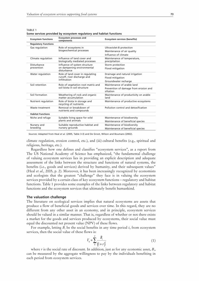
Valuation of ecosystem services supporting aquatic and other land-based food systems 71 Edward B. Barbier

Use of life cycle assessment (LCA) to compare the environmental impacts of aquaculture and agri-food produc 87 Rattanawan Mungkung and Shabbir H. Gheewala

The potential use of the Materials and Energy Flow Analysis (MEFA) framework to evaluate the environmental costs of agricultural production systems and possible applications to aquaculture 97Helmut Haberl and Helga Weisz

Considerations for comparative evaluation of environmental costs of livestock and salmon farming in southern Chile 121Doris Soto, Francisco J. Salazar and Marta A. Alfaro

Assessing the environmental costs of Atlantic salmon cage culture in the Northeast Pacific in perspective with the costs associated with other forms of food production 137Kenneth M. Brooks

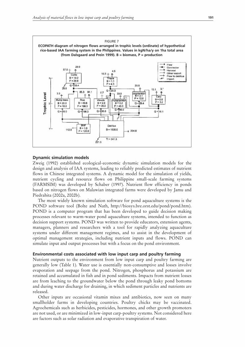
Comparative analysis of material flows in low input carp and poultry farming: an overview of concepts and methodology 183Mark Prein

Exploratory analysis of the comparative environmental costs of shrimp farming and rice farming in coastal areas 201John W. Gowing and Patricia Ocampo-Thomason

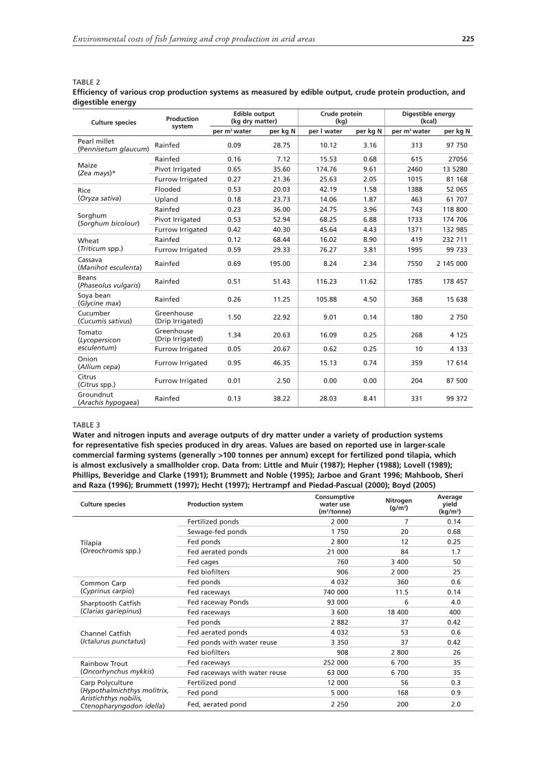
Comparative analysis of the environmental costs of fish farming and crop production in arid areas 221Randall E. Brummett

Biophysical accounting in aquaculture: insights from current practice and the need for methodological development 229Peter Tyedmers and Nathan Pelletier

1

Genesis of the workshop

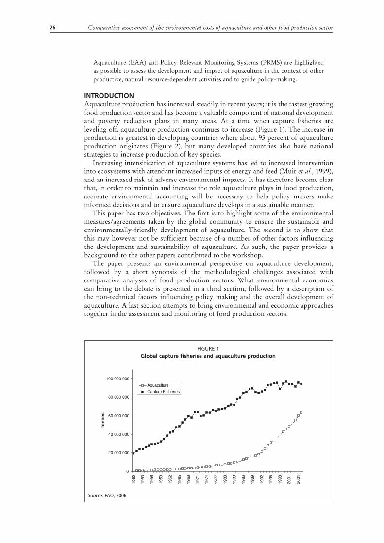
The projected global demand for fish and fish products is expected to increase over the next decade. Because many capture fisheries are at their limits of production and the energy requirements to run the world’s fisheries are increasing in spite of technological improvements in fishing, satisfying this demand will rely on increased production from aquaculture. Aquaculture is now one of the fastest-growing food-producing sectors, but it is being criticized for creating adverse environmental impacts. In order to maintain the growth of aquaculture and protect the environment, accurate environmental accounting of food production will be necessary to help policy-makers make informed decisions that will ensure aquaculture develops in a responsible manner.

The international community recognizes the need to address the environmental impacts of development. The Convention on Biological Diversity (CBD) and the FAO Code of Conduct for Responsible Fisheries (CCRF) are key international instruments that have called for development to address environmental concerns and strive to protect natural biological diversity. In acknowledging the adverse environmental impacts from the food production sector, the First Session of the FAO Committee on Fisheries’ Sub-Committee on Aquaculture held in Beijing, China, from 18 to 22 April 2002, recommended future work be devoted to “undertaking comparative analyses on the environmental cost of aquatic food production in relation to other terrestrial food production sectors”. The Sub-Committee specifically asked the FAO Fisheries and Aquaculture Department to undertake such a study and analysis.

The workshop reported here (Annex 1) is a first step to address that request. Its purpose was to provide FAO with information that could be used to advise Members on how to make development decisions that take into account the environmental costs of food production. These decisions will help determine where public and private sector investments will help optimize national food production in terms of economic viability, environmental sustainability and social acceptability. FAO’s ultimate aim would be to minimize adverse costs and impacts of food production systems through facilitating informed decisions at the national level.

To that end, a group of experts in aquaculture development, ecology, environmental economics, environmental impact analysis, energy analysis and livestock farming (Annex 2) were brought together to advise FAO on appropriate and accurate accounting approaches for comparing environmental costs of aquaculture and other terrestrial food production sectors; to evaluate the strengths and weaknesses of these accounting systems; and to advise FAO on options for moving forward in this important area. While the workshop recognized that social aspects of environmental impacts are extremely important and should be considered in analyses and in decision-making, this area was not addressed in sufficient detail to provide meaningful statements. Similarly, traditional economic impact analysis was not discussed in detail, despite clearly having application in cost-benefit analysis.

3

Food production: intensification and environmental impacts

Aquaculture may be the fastest growing food-producing sector but others are increasing as well. Consumption of animal products in the developing world rose from 15 kg per capita in 1982 to 28 kg per capita in 2002 and is expected to reach 37 kg by 2030 (Gerber et al., 2007; Soto, Salazar and Alfaro, 2007; FAO, 2004); this is nearly twice as high as predicted consumption of food from aquatic sources. Food production has in general outpaced human population growth over the last few decades but the distribution of this increased production is still inequitable (FAO, 2002).

A key driver of the increase in food production is intensification of farming systems, often characterized by increased inputs, effluents and energy demands (Prein, 2007). However, more traditional farming systems that use large amounts of land may also pose serious risks to the environment, native biodiversity and local communities. Evaluation of these risks has been attempted, but assessment has not generally included comprehensive analysis of costs to the environment, and there have been very few studies done comparing different food production sectors.

Yet all development has impacts. Progress has been made in mitigating some of them, but there is a long way to go. Production of feed has been identified as one of the most significant environmental and economic costs in both the aquaculture and livestock sectors. While farmed aquatic animals are generally more efficient converters of feed energy than are ruminants, many farmed aquatic animals are fed diets with fishmeal and fish oil. This has led to criticism of the aquaculture sector for using fish to feed fish and for causing environmental problems. Reducing the fishmeal and fish oil component in aquaculture feeds is a high priority for intensive systems; in salmon feeds, for example, some current formulations rely much less on wild fishmeal than did diets of a decade ago with a reduction from 60 to 35 percent (Tacon, 2005). The energy needs of fish farming may thus be reduced along with the dependence on fish products in the feed. However the global growth of aquaculture and the increasing use of formulated feeds present a challenge as there is a net increase in total demand for fishmeal and fish oil.

The important role of the environment in providing ecosystem services is becoming better understood, sometimes with surprising results. For example, while mangroves provide valuable feeding and nursery areas for many coastal fisheries, their value in protecting coastal communities from storm damage may in fact be greater (Barbier, 2007).

Because development agencies may need to consider a range of development or resource management scenarios, the analytical process upon which these scenarios are based should include comparison of the costs of all potential options. Comparative environmental cost assessment is therefore not only an important and potentially fertile area for study, it is also an area where research results will be extremely useful to decision-makers, the industry and the public. Nevertheless, misconceptions concerning food production and its impacts persist. These misconceptions, as well as the general lack of knowledge concerning food production and the environment, can only be eliminated through policies that are informed by science-based studies.

5

Workshop findings

The present workshop represented a scoping exercise which identified broad issues that need to be addressed in environmental cost analysis. Further action will be needed to move the analyses forward in order to promote food production systems that are economically viable, environmentally sustainable and socially acceptable.

THE NEED FOR A LEVEL PLAYING FIELDThe main conclusion of the workshop was that it is necessary to include environmental costs in any analysis of the sustainability of any food-producing sector. This message is certainly not new. The concept of “sustainable development” was explicitly identified 20 years ago in the Brundtland Report (UNGA, 1987); however, sustainability has been difficult to achieve or simply ignored. Fortunately, the tools available to address the issue are better now; unfortunately, policy- and decision-makers may still avoid using them if the result is politically unpalatable. There is thus a need to present a balanced picture of the environmental costs of all food-producing sectors and to formulate environmental policies that deal with the impacts of all sectors. Such a balanced view will require a multidisciplinary team of ecologists, economists, social scientists and policy-makers working with the appropriate food production sectors. The ultimate goal should be to balance all development sectors, e.g. tourism, municipal development and capture fisheries.

So long as this balanced picture of environmental costs is absent, policy does not reflect farming realities, the prices of food products cannot reflect the real costs of their production, especially for ecosystems and communities, and both the public and government receive very mixed messages. Inconsistencies become common. For example, the recent explosion of aquaculture has led in some cases to overregulation, while other sectors with a longer history of production have negative impacts that have traditionally been accepted (Brooks, 2007; Gowing and Ocampo-Thomason, 2007; Soto, Salazar and Alfaro, 2007).

IS THERE OVERREGULATION OF AQUACULTURE?The workshop identified two main reasons why aquaculture may be subject to more regulation than other sectors, at least in some parts of the world. First, aquaculture is relatively new, and growing rapidly. That growth impinges on established uses of land and water: hotels, farms, housing developments, industry etc. may already be established near water bodies where aquaculture is proposed or already being developed. These previously established activities have already been accepted by society; adding aquaculture to the picture invites additional scrutiny and criticism. People have become accustomed to and may even prefer seeing lighted city streets or rolling pastures, but cages in the sea may not be so palatable. Such preferences can easily affect government policy.

Second, farming and other terrestrial development often use private land with well-defined boundaries and access rights. The aquaculture ventures that are most often criticized or heavily regulated are marine and coastal operations located on common property where boundaries and access rights are less well defined and impacts more difficult to contain.

There may also be misconceptions regarding the science on which regulations are based. For example, use of certain pesticides is highly restricted in the United Kingdom of Great Britain and Northern Ireland, but these pesticides have been shown to have

Comparative assessment of the environmental costs of aquaculture and other food production sector6

minimal effects in that country (Gowing and Ocampo-Thomason, 2007). Nutrient inputs are also regulated in waters of the Pacific Ocean around Chile and also around the Canada/United States of America border. However, some studies have shown the specific nutrients being regulated to have little adverse impact in these environments (Brooks, 2007; Soto, Salazar and Alfaro, 2007). Thus, the industry may feel that regulation does not always address the real causes of environmental perturbations.

Despite these controversies, there is no question that environmental effects have been identified and all food-producing sectors need to mitigate them. Industry needs to be aware that the costs of avoiding or pre-treating hazards are often much lower than the penalties for non-compliance or the costs of cleanup or rehabilitation (e.g. mangrove replanting; Brooks, 2007; Soto, Salazar and Alfaro, 2007).

EFFECTS OF ECONOMIC AND TECHNOLOGICAL GROWTH AND PUBLIC PERCEPTIONThe workshop discussed whether economic growth is a prerequisite to managing environmental issues and mitigating adverse impacts (Brugère, Soto and Bartley, 2007). The relationship between economic growth (national income) and environmental degradation or some of its components (e.g. pesticide use) can be expressed mathematically and suggest that pollution associated with production activities decrease after a certain level of income has been reached. The relationship is complicated, however, and is affected by technological progress, relative energy prices and the presence of adequate and well-functioning institutions (Brugère, Soto and Bartley, 2007).

Another aspect complicating analyses of environmental costs is that food production systems keep changing; intensification and the use of genetically modified plants and animals are good examples. Change in the industry means that government and public perception and acceptance of farmed products are changing too. The rise in popularity of organic products, the controversy over the health and environmental effects of farmed salmon in some developed countries, the reluctance to use genetically modified fish in aquaculture, and the increased value being placed on native biodiversity are all examples of attitudes that are anything but static. In developed countries, cost may not be the most important factor: although consumers often express a preference for inexpensive food products, the rise in demand for organic products indicates that some people are willing to pay more for a product they perceive to be more environmentally or socially friendly. Therefore, there should be periodic reassessment of models and analyses that compare trade-offs between environmental impacts, consumer preferences and production efficiencies.

THE NEED FOR COMMUNICATIONThe pace of technological and social change implies that good policies on the environmental costs of food production can only come about where there is good communication. Misconceptions concerning the impact of certain effluents, the overregulation of a sector because it is the most recent, the failure to appreciate the cost-savings of early prevention of adverse impacts, the failure to place adequate value on biodiversity and ecosystem services, and the changing nature of food production are all issues that demand the sharing of information. That information will need to be packaged for three key groups: policy-makers, farmers (including aquaculturists) and consumers. A key component of that information will be provided by the methods for economic and environmental analysis discussed in the following section.

COMPARISON OF THE EXISTING METHODS FOR ASSESSING ENVIRONMENTAL COSTS OF FOOD PRODUCTION The workshop identified numerous problems that arise when one attempts to compare environmental costs of different food production sectors. These problems stem from:

7

• the many differences between terrestrial and aquatic environments;• differences in patterns of ownership, e.g. terrestrial areas are often privately

owned while aquatic areas are often common property;• the huge diversity of farmed products;• the need to choose a functional unit for comparison, e.g. kg of protein, energy,

contribution to daily nutrient or energy requirements;• the difficulty of translating impacts into monetary units;• the diversity in farming systems within a given sector, e.g. feed-lot to free range

livestock, and small-scale extensive to super-intensive aquaculture;• the influence of management practices on environmental impacts and costs of

production; and• differences in terminology between sectors and disciplines, e.g. “sustainability”

and “cost” have different meanings for ecologists and economists, while “water productivity” would be defined differently by fisheries biologists and water management engineers.

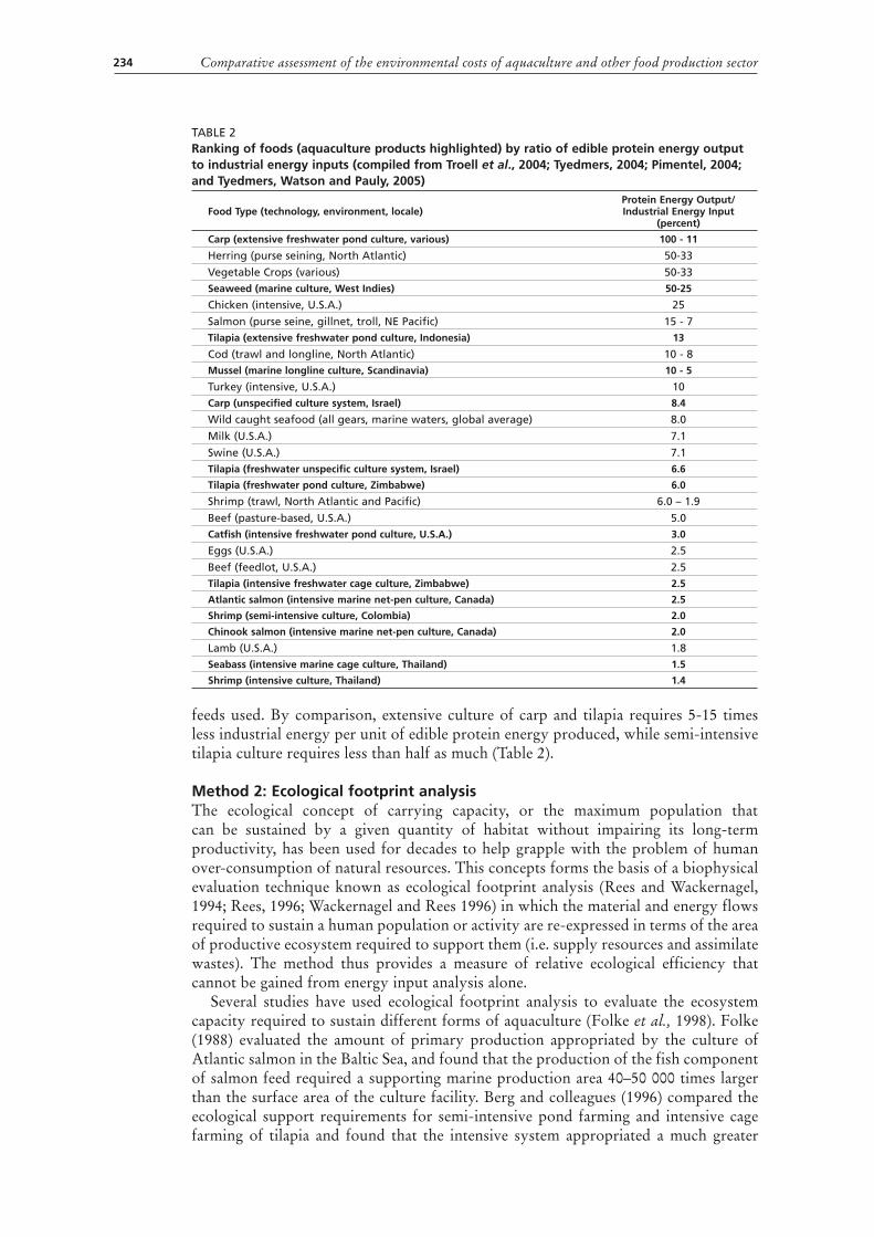
Nevertheless, valid comparisons can be useful to address local development and zoning concerns, global issues of sustainability and trade, and consumer preferences for inexpensive food produced in an environmentally sustainable manner. The workshop developed a general framework for assessing the environmental costs of food production (Annex 3). Although few comparisons have been reported, they can be done when the systems are well defined and data are available (Brooks, 2007; Brummet, 2007; Gowing and Ocampo-Thomason, 2007). Biophysical methods have a history of use and corresponding data on energy equivalents of certain activities that can be linked to methods such as Life Cycle Analysis (LCA) (Mungkung, 2007; Tyedmers and Pelletier, 2007) and material and energy flow analyses (Prein, 2007; Haberl and Weisz, 2007) to allow comparisons of different impacts or costs.

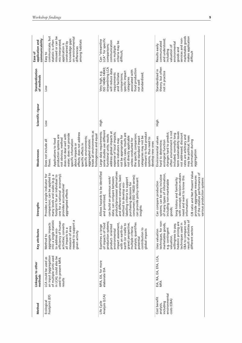
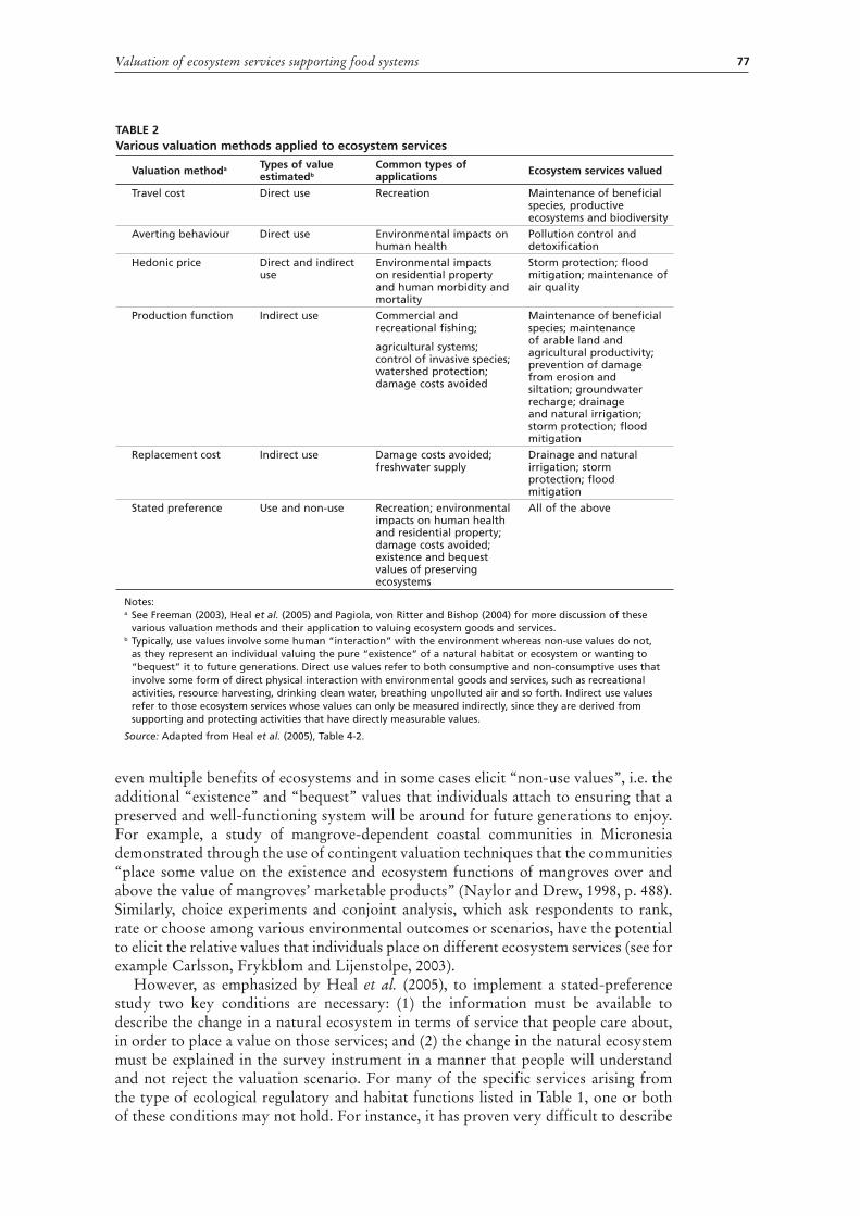
A wide range of methods has been developed in order to assess environmental costs of development (Table 1). Each has its own strengths and weaknesses. Because environmental valuation is often omitted in analyses of any of the food sectors, many of the “external costs” referred to earlier are presently not well accounted for in these methods (Barbier, 2007). In order to be useful to FAO and decision-makers, methods to assess environmental costs must not only include these externalities but should also be scientifically-based, comparable across different sectors, expandable to different scales, practical to implement and able to produce results that are easily understood and interpreted. Satisfying all these criteria will be difficult; trade-offs and combinations of methods will need to be made.

The workshop concluded that none of the existing methods captures all of environmental impacts and costs of food production. With the possible exception of Environmental Impact Assessment (EIA) and Cost-Benefit Analysis (CBA), few decisions can be made using a single method. However, many of the methods can and should be used together, and various combinations may be fruitful. For example, LCA and Material Flows Accounting (MFA) can first identify key sources of pollution, then environmental valuation and CBA can be applied to the specific environment or commodity to determine which development path to take.

Existing legislation often specifically mandates the use of EIA. Although EIA is better than nothing (and in many cases there really is no assessment at all) it may be inappropriate or incomplete in some circumstances. Risk assessment (RA, see Brooks, 2007) is another method that may also provide incomplete analyses. These two methods used alone usually do not include environmental valuation criteria, and it would be preferable to complement them with other methods that include multiple criteria and environmental valuation. There are some issues common to all methods: the need for accurate information, the problem of assigning values to un-marketed goods such as environmental goods and ecosystem services, and the problem of biased analysis.

Workshop findings


TAB

LE 1

Co

mp

aris

on

of

met

ho

ds

for

envi

ron

men

tal c

ost

an

alys

is

Met

ho

d

Lin

kag

es t

o o

ther

m

eth

od

sK

ey a

ttri

bu

tes

Stre

ng

ths

Wea

knes

ses

Scie

nti

fic

rig

ou

rSt

and

ard

izat

ion

o

f m

eth

od

s

Ease

of

app

licat

ion

an

d

com

mu

nic

abili

tyEn

viro

nm

enta

l Im

pac

t A

sses

smen

t (E

IA)

CB

A, R

APr

oje

ct-b

ased

, d

escr

ipti

ve, s

ite-

spec

ific

Pub

lic p

lan

nin

g a

nd

tra

nsp

aren

t p

roce

ss;

bas

ed o

n m

ult

iple

cri

teri

a an

d c

an b

e u

sed

in s

ensi

tivi

ty

anal

ysis

;

iden

tifi

es h

azar

ds

and

imp

acts

; al

low

s re

des

ign

of

pro

ject

to

re

du

ce im

pac

ts.

Do

es n

ot

qu

anti

fy t

rad

e-o

ffs

or

effe

cts:

do

es

no

t p

rovi

de

a si

ng

le

per

form

ance

ind

icat

or

for

com

par

iso

ns;

p

rob

lem

s w

ith

ho

w t

o

inte

rpre

t d

ata

Var

iab

le (

very

hig

h

to lo

w);

lots

of

un

cert

ain

ty d

ue

to

lack

of

dat

a; o

ften

ti

me-

con

stra

ined

d

ue

to d

evel

op

men

t d

ead

lines

Hig

h (

e.g

. Eu

rop

e) b

ut

may

var

y ac

ross

se

cto

rs, r

egio

ns

and

in n

atio

nal

le

gis

lati

on

Go

od

; oft

en

fig

ure

s p

rom

inen

tly

in

dec

isio

n-m

akin

g

Ris

k A

sses

smen

t o

r A

nal

ysis

(R

A)

Sho

uld

un

der

pin

all

oth

er m

eth

od

s fo

r h

azar

d id

enti

fica

tio

n

and

un

der

stan

din

g;

wid

ely

use

d in

to

xici

ty

anal

ysis

Too

l fo

r u

nd

erst

and

ing

en

viro

nm

enta

l p

roce

sses

Co

ntr

ibu

tes

to b

ette

r u

nd

erst

and

ing

of

envi

ron

men

tal f

low

s an

d

imp

acts

: att

emp

ts t

o b

e q

uan

tita

tive

bu

t ca

n a

lso

be

qu

alit

ativ

e; id

enti

fies

haz

ard

s an

d im

pac

ts.

Rel

ies

on

qu

alit

ativ

e ju

dg

emen

ts a

nd

es

tim

ates

du

e to

kn

ow

led

ge

gap

s;

limit

ed c

om

par

ativ

e u

se

(so

me

risk

s ap

ply

to

so

me

sect

ors

, oth

ers

no

t)

Var

iab

le a

t p

rese

nt;

q

uan

tita

tive

m

easu

res

nee

d

to b

e d

evel

op

ed

(en

viro

nm

enta

l in

dic

ato

rs)

Hig

h f

or

pro

ced

ura

l as

pec

ts

Go

od

; fo

rmal

ized

in

leg

isla

tio

n a

s d

ecis

ion

-mak

ing

to

ol

Mat

eria

l Flo

ws

Acc

ou

nti

ng

(M

FA),

Mas

s b

alan

ce, a

nd

In

pu

t/O

utp

ut

mo

del

s (I

O)

A f

irst

ste

p t

ow

ard

s m

ore

co

mp

lete

as

sess

men

ts u

sin

g E

IA,

RA

, en

erg

y an

alys

is

Exam

ines

inp

ut

and

ou

tpu

t o

f ke

y m

ater

ials

; acc

ou

nts

fo

r b

iolo

gic

al f

low

s as

soci

ated

wit

h

eco

no

mic

act

ivit

ies;

ap

plic

able

to

sys

tem

s at

man

y sc

ales

Qu

anti

fies

leve

ls o

f in

pu

ts

and

ou

tpu

ts; c

an p

rod

uce

co

mp

arab

le in

form

atio

n

ove

r ti

me

and

sp

ace;

use

d t

o

imp

rove

eco

log

ical

eff

icie

ncy

; w

ell-

kno

wn

to

ol w

ith

sta

nd

ard

p

roto

cols

.

Do

es n

ot

refl

ect

envi

ron

men

tal e

ffec

ts;

snap

sho

t p

ictu

re o

f fl

ow

s at

a s

pec

ific

po

int

in t

ime

and

pla

ce.

Hig

hH

igh

Ver

y g

oo

d

Ener

gy

anal

ysis

(E

A)

Co

uld

be

inco

rpo

rate

d

into

MFA

an

d u

sed

co

mp

lem

enta

rily

wit

h

CB

A

Exam

ines

fo

ssil

fuel

en

erg

y u

sed

in f

oo

d

pro

du

ctio

n

Pro

du

ces

a si

ng

le m

easu

re,

wh

ich

is a

pro

xy f

or

the

oth

er

com

po

nen

ts o

f th

e se

cto

r, fo

r co

mp

aris

on

; go

od

his

tory

of

anal

ysis

an

d d

ata;

co

mp

arab

le

at a

ll le

vels

.

Pres

ents

an

inco

mp

lete

p

ictu

re o

f th

e se

cto

r;

rele

van

ce is

qu

esti

on

ed

bec

ause

en

erg

y (f

uel

) h

as a

mar

ket

valu

e th

at w

ill c

han

ge;

do

es

no

t ac

cou

nt

for

the

envi

ron

men

tal e

ffec

ts o

f fu

el c

on

sum

pti

on

.

Hig

hH

igh

Go

od

; few

d

ecis

ion

s ar

e m

ade

on

EA

alo

ne

Hu

man

A

pp

rop

riat

ion

o

f N

et P

rim

ary

Pro

du

ctiv

ity

(HA

NPP

)

Can

be

use

d w

ith

M

AF,

EA

, EF

An

ind

icat

or

of

envi

ron

men

tal

effe

cts

bas

ed

on

ch

ang

es in

ec

olo

gic

al f

low

s o

f tr

op

hic

en

erg

y ca

use

d b

y la

nd

use

Ag

gre

gat

es in

form

atio

n in

to a

si

ng

le s

tati

stic

fo

r co

mp

aris

on

, e.

g. l

and

use

ch

ang

e; c

an

exam

ine

eco

no

mic

cau

ses

for

chan

ge;

eco

log

ical

ly f

ocu

sed

in

dic

ato

r; c

om

par

able

at

dif

fere

nt

scal

es, r

egio

ns

and

ac

ross

tim

e

No

t w

ell d

evel

op

ed f

or

aqu

atic

en

viro

nm

ents

; d

oes

no

t d

escr

ibe

imp

acts

an

d d

oes

no

t ad

dre

ss

spec

ific

loca

l eco

log

ical

ch

ang

es; l

imit

ed e

xper

tise

fo

r H

AN

PP a

nal

ysis

; in

so

me

case

s an

alys

is o

f se

con

dar

y o

r te

rtia

ry

pro

du

ctiv

ity

wo

uld

be

mo

re in

form

ativ

e

Hig

hM

ediu

m

Easy

to

co

mm

un

icat

e;

dif

ficu

lt t

o

inte

rpre

t

9

Met

ho

d

Lin

kag

es t

o o

ther

m

eth

od

sK

ey a

ttri

bu

tes

Stre

ng

ths

Wea

knes

ses

Scie

nti

fic

rig

ou

rSt

and

ard

izat

ion

o

f m

eth

od

s

Ease

of

app

licat

ion

an

d

com

mu

nic

abili

ty

Eco

log

ical

Fo

otp

rin

t (E

F)LC

A c

ou

ld b

e u

sed

as

an in

pu

t (a

gg

reg

atio

n

of

mu

ltip

le u

nit

s u

sed

in

LC

A);

co

uld

als

o b

e u

sed

to

pre

sen

t M

FA

resu

lts

Met

ho

d t

o

agg

reg

ate

imp

acts

in

to a

sin

gle

sta

tist

ic

to a

dd

ress

eco

-ef

fici

ency

of

hu

man

ac

tivi

ties

; co

nve

rts

all i

mp

acts

to

a

mea

sure

of

area

n

eed

ed t

o s

up

po

rt a

g

iven

act

ivit

y

Pro

vid

es a

sin

gle

ind

icat

or

for

com

par

iso

n; c

an b

e ap

plie

d t

o

man

y le

vels

an

d s

cale

s (e

.g. a

fo

otp

rin

t fo

r an

ind

ivid

ual

to

o

ne

for

a n

atio

nal

ec

on

om

y);

pro

vid

es a

ccu

mu

lati

ve/

agg

reg

ated

eff

ects

Do

es n

ot

incl

ud

e al

l fl

ow

s.

Ap

plic

atio

ns

to f

oo

d

pro

du

ctio

n s

yste

ms

are

no

t o

bvi

ou

s; m

eth

od

d

oes

no

t d

eal w

ell w

ith

w

ater

; do

es n

ot

pro

vid

e sp

ecif

ic in

form

atio

n

abo

ut

imp

acts

or

effe

cts;

do

es n

ot

add

ress

sp

ecif

ic e

ffec

ts in

sp

ecif

ic e

nvi

ron

men

ts;

agg

reg

ated

sta

tist

ic

trea

ts a

ll en

viro

nm

ents

as

ho

mo

gen

ou

s an

d e

qu

al

Low

Low

Easy

to

co

mm

un

icat

e, b

ut

stat

isti

c is

oft

en

mis

use

d o

r ca

n b

e m

is-i

nte

rpre

ted

; ap

plic

atio

n is

co

nst

rain

ed b

y kn

ow

led

ge

gap

s o

n e

nvi

ron

men

tal

dif

fere

nce

s am

on

g h

abit

ats

Life

Cyc

le

An

alys

is (

LCA

) M

FA, E

A, f

or

mo

re

elab

ora

te E

IA

Exam

ines

a r

ang

e o

f im

pac

ts o

f fo

od

p

rod

uct

ion

sys

tem

s;

pro

du

ct-

ori

ente

d

envi

ron

men

tal

imp

act

asse

ssm

ent,

w

ith

an

ear

th-t

o-

eart

h (

or

crad

le t

o

gra

ve)

per

spec

tive

, m

ult

iple

cri

teri

a an

alys

is; q

uan

tifi

es

po

ten

tial

co

ntr

ibu

tio

n t

o

glo

bal

imp

acts

Allo

ws

haz

ard

s to

be

iden

tifi

ed

and

pri

ori

tize

d;

can

bu

ild o

n p

revi

ou

s w

ork

/d

ata;

can

co

mp

are

bet

wee

n

pro

du

cts/

pro

cess

es/ a

lter

nat

ives

an

d d

iffe

ren

t sc

enar

ios;

bas

ic

met

ho

d t

o d

evel

op

eco

-la

bel

ling

cri

teri

a to

su

pp

ort

p

urc

has

ing

dec

isio

ns

for

con

sum

ers

(ISO

140

20 s

erie

s);

can

pro

vid

e p

olic

y-re

leva

nt

insi

gh

ts

Larg

e d

ata

req

uir

emen

ts;

som

e st

ud

ies

use

dif

fere

nt

fun

ctio

nal

un

its;

res

ult

s ad

dre

ss g

lob

al im

pac

ts a

t ex

pen

se o

f lo

cal i

mp

acts

; so

me

ind

icat

ors

may

n

ot

be

app

rop

riat

e fo

r sp

ecif

ic c

ases

; res

ult

s ar

e n

ot

dir

ectl

y ap

plic

able

u

nle

ss c

on

du

cted

fo

r th

e sp

ecif

ic c

om

par

iso

n;

som

e st

and

ard

imp

act

cate

go

ries

may

no

t b

e re

leva

nt

to f

oo

d p

rod

uct

sy

stem

s, t

hu

s n

eed

to

d

evel

op

new

on

es

Hig

hV

ery

hig

h, e

.g.

ISO

140

40-1

4043

; st

ream

linin

g L

CA

w

ill r

edu

ce d

ata

req

uir

emen

ts

and

fac

ilita

te

com

par

iso

ns;

sp

ecif

ic im

pac

t ca

teg

ori

es

asso

ciat

ed w

ith

fo

od

pro

du

ctio

n

no

t w

ell

stan

dar

diz

ed;

Can

“st

ream

line

LCA

” fo

r sp

ecif

ic

com

par

iso

ns;

co

mm

un

icat

ion

o

n m

ult

iple

cr

iter

ia m

ay b

e d

iffi

cult

;

Co

st b

enef

it

anal

ysis

, in

clu

din

g

envi

ron

men

tal

cost

s (C

BA

)

EIA

, RA

, EA

, EFA

, LC

A,

MFA

Use

s va

luat

ion

te

chn

iqu

es, f

or

no

n-

mar

keta

ble

go

od

s,

e.g

. co

nti

ng

ent

valu

atio

n,

will

ing

nes

s to

pay

, h

edo

nic

pri

cin

g a

re

tech

niq

ues

use

d in

C

BA

to

co

mp

are

net

re

sult

of

acti

viti

es o

f d

iffe

ren

t se

cto

rs

Can

co

mp

are

pro

du

ctio

n

syst

ems;

can

be

very

incl

usi

ve

of

man

y ty

pes

of

info

rmat

ion

, in

clu

din

g n

on

-mar

keta

ble

g

oo

ds;

lon

g h

isto

ry a

nd

fam

iliar

ity

wit

h c

on

cep

t; d

ecis

ion

-mak

ers

nee

d a

nd

wan

t to

kn

ow

th

is

info

rmat

ion

;

C/B

rat

io a

nd

Net

Pre

sen

t V

alu

e

pro

vid

e ag

gre

gat

e m

easu

res

of

the

rela

tive

per

form

ance

of

vari

ou

s p

rod

uct

ion

sys

tem

s

Envi

ron

men

tal v

alu

es

har

d t

o d

eter

min

e;

eco

log

ical

fu

nct

ion

ch

ang

es h

ard

to

pre

dic

t;

oft

en e

nvi

ron

men

t is

no

t in

clu

ded

; no

rmal

ly lo

ng

te

rm s

ust

ain

abili

ty is

sues

n

ot

add

ress

ed; d

isco

un

t ra

tes

are

arb

itra

ry a

nd

m

ay b

e p

olit

ical

; lo

ses

info

rmat

ion

du

rin

g

agg

reg

atio

n

Hig

hSt

and

ard

ized

in

theo

ry, b

ut

oft

en

no

t in

pra

ctic

e

Res

ult

s ea

sily

co

mm

un

icat

ed

and

un

der

sto

od

; in

clu

din

g

valu

atio

n o

f en

viro

nm

enta

l g

oo

ds

and

se

rvic

es a

nd

no

n-

mar

keta

ble

go

od

s m

akes

ap

plic

atio

n

dif

ficu

lt

Workshop findings


The workshop noted that application or interpretation of the results of any of these methods could be affected by development context. A developer who is responsible for cost analysis certainly has a stake in the results of the analysis. However, bias is spread between all parties (including academics industry and conservation groups) – which is why methods and their environmental, social, and economic results need to be reviewed by a multidisciplinary team.

IDENTIFYING THE MOST IMPORTANT IMPACTSThe methods provide a basic framework for analysis and impact assessment. An initial step in the framework is the identification of the hazards or adverse impacts for the sectors where valuation of environmental damage is to be compared. Those hazards or impacts need to be described in terms of probability and consequences. It is clearly important to choose impacts that will provide the most useful comparative analysis. Impacts can be classified using the following criteria (Brooks, 2007):

• amount of adequate data to address the issue;• probability of the hazard or impact occurring;• consequences if it does occur; and• level of confidence in the analysis, i.e. level of uncertainty.Using these criteria, a suite of potential hazards can be narrowed down for

comparative analysis. This is similar to standard procedures in risk analysis.

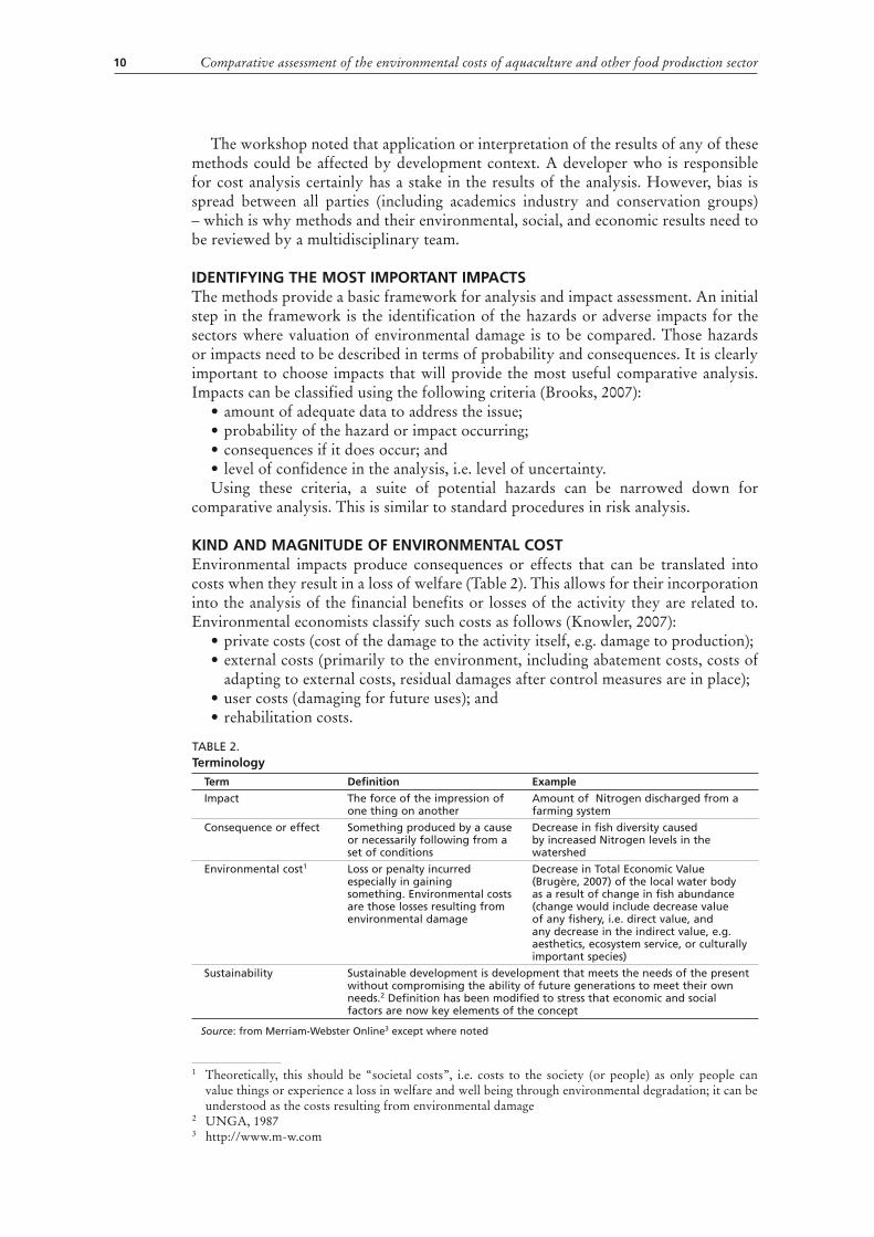
KIND AND MAGNITUDE OF ENVIRONMENTAL COSTEnvironmental impacts produce consequences or effects that can be translated into costs when they result in a loss of welfare (Table 2). This allows for their incorporation into the analysis of the financial benefits or losses of the activity they are related to. Environmental economists classify such costs as follows (Knowler, 2007):

• private costs (cost of the damage to the activity itself, e.g. damage to production);• external costs (primarily to the environment, including abatement costs, costs of

adapting to external costs, residual damages after control measures are in place);• user costs (damaging for future uses); and• rehabilitation costs.

TABLE 2.Terminology

Term Definition Example

Impact The force of the impression of one thing on another

Amount of Nitrogen discharged from a farming system

Consequence or effect Something produced by a cause or necessarily following from a set of conditions

Decrease in fish diversity caused by increased Nitrogen levels in the watershed

Environmental cost1 Loss or penalty incurred especially in gaining something. Environmental costs are those losses resulting from environmental damage

Decrease in Total Economic Value (Brugère, 2007) of the local water body as a result of change in fish abundance (change would include decrease value of any fishery, i.e. direct value, and any decrease in the indirect value, e.g. aesthetics, ecosystem service, or culturally important species)

Sustainability Sustainable development is development that meets the needs of the present without compromising the ability of future generations to meet their own needs.2 Definition has been modified to stress that economic and social factors are now key elements of the concept

Source: from Merriam-Webster Online3 except where noted

1 Theoretically, this should be “societal costs”, i.e. costs to the society (or people) as only people can value things or experience a loss in welfare and well being through environmental degradation; it can be understood as the costs resulting from environmental damage

2 UNGA, 19873 http://www.m-w.com

11

In comparative environmental cost analysis it is important to define the scale and scope of the system analyzed, including outstanding issues and the overall purpose of the analysis. Results of analyses need to be placed in the proper perspective, i.e. the results need to stated in terms of real changes to the environment, so that the consequences of different comparisons can be estimated (Knowler, 2007). Simply reporting the presence of X kg of Y nutrient in Z environment is meaningless unless the environmental consequences of the inputs are specified (Brooks, 2007). Analyses need also to include information on the consequences to the environment and a valuation of the resulting loss of ecosystem products and services – a complicated task that is rarely undertaken.

CHOOSING UNITS FOR COMPARISONComparative analysis requires normalization of the unit of assessment (Brummet, 2007; Mungkung and Gheewala, 2007) as well as the scope of the consequences to be contemplated. For example, LCA usually examines global consequences and therefore may be unsuited to determining impacts on a specific ecosystem. Analyses have often reported production as simple kilograms of product, but a kilogram of shrimp has very different nutritional and monetary values from a kilogram of chicken and corn. Some candidate units that these data could be converted to include edible output, crude protein or digestible energy equivalents (Brummet, 2007; Mungkung and Gheewala, 2007).

However, farming is above all a business that produces food to generate money. Farming systems that produce a high value product may be able to produce less while meeting economic objectives (thereby using less inputs); they may also be able to meet production objectives using intensive systems with minimal effluents, thereby having less environmental impact than extensive systems grown over a large area to produce a large amount of low value product. When comparing such sectors, conversion of product and costs into monetary units may be advisable. It is also important to keep in mind the overall objectives of the farming system, especially when comparisons of environmental costs are being made. For example, farming can increase food security, but the money it also generates can buy more food as well.

TRADE-OFFS AND FAIR COMPARISONSMany things cannot be usefully (or fairly) compared because of the differences in the commodity or the environment in which it is produced. Thus comparing the environmental costs of producing beef from a feedlot in Chile with production of tilapia in Thailand would be pointless for national policy-makers, but might be relevant for consumers who wish to know which production system has a greater influence on climate change.

In comparing aquaculture and livestock, the feed used by both sectors has a strong influence on their environmental costs. For example, the environmental costs of salmon farming become high when the costs of catching fish and processing them into fishmeal and fish oil are included, because wild populations of fish are reduced and energy expended in catching and processing them. Similarly, the water and fertilizer requirements for beef production are high when the costs of producing feed are included because the water is lost to other uses or ecosystem services, and production of fertilizer expends energy.

Comparisons should facilitate the kinds of real choices policy-makers and the consumer need to make. Decisions at the national and local levels will justifiably be based on societal needs, priorities and preferences (CBD, 1994). There will usually be trade-offs between economic gains and environmental costs and therefore a need for multicriteria decision analysis methods that prioritize benefits and costs (Mungkung and Gheewala, 2007). In such analyses, methods that include a suite of characters (e.g.

Workshop findings


LCA, MFA) rather than aggregated single measures or indices (e.g. ecological footprint and CBA) will generate more accurate comparisons.

INFORMATION AND COMMUNICATION NEEDSComparative analyses will require extensive information on farm production and effluent, material flows, prices, biodiversity affected by farming, ecosystem products and services and economics. Some of this basic information is available free of charge over the internet or by request, for example the FAO databases on livestock, fisheries and aquaculture production, land use, and food balance sheets. FishBase4 contains information on most of the world’s fishes. Other information is available for a fee, e.g. Ecoinvent5 or satellite data. Information on local biodiversity or production on private farms is often non-existent or difficult to access; for example, information on illegal farming practices such as the use of banned drugs is crucial to impact analysis, but by its very nature is difficult to obtain. There is usually a wealth of useful information in government files or in older literature that is often forgotten or not published in popular or scientific media; some comparisons could be made through specific desk studies using this grey literature.

A distinction must be made between simple lack of data and the uncertainties that are either contained within the data that do exist or inherent in the task of making predictions about far-flung biological effects. An example of the former would be information gaps on the carrying capacity of coastal ecosystems, or levels of effluent from various types of farms. An example of the latter is in the basic values of environmental goods and services. This is partly due to differences of opinion on how to assign values to intangibles such as endangered species and ecosystem services; nevertheless, data are accumulating to indicate that these services are very valuable (Barbier, 2007). Information from biophysical analysis does exist and there are additional sources of information that can be used in evaluating impacts and costs. More fundamental uncertainty would surround the long-term ecosystem consequences of environmental impacts, the area of uncertainty judged by the workshop to be the most serious.

It should be recognized that a “complete” set of all the relevant scientific information will never be available and that comparative analyses may need to be done with the best at hand. We already have general knowledge of production systems, their probable outputs and possible effects (Brummet, 2007) and should not let the incompleteness of such information stand in the way of analyses of food production sectors.

After analyses have been completed, results will need to be communicated to a variety of groups. These include:

• policy-makers (to establish environmental regulations, environmental impact mitigation measures, and for zoning of aquaculture/agriculture);

• farmers (to help plan production, understand and comply with environmental regulations, and implement good management practices); and

• consumers (to help make informed choices on food production and drive appropriate policy and farming practices).

Each of the above groups has different backgrounds, mindsets and agendas, so the language and vehicles used to communicate research results will be different for each.

4 http://www.fishbase.org 5 http://www.ecoinvent.ch

13

A potential role for FAO

It is only recently that FAO in general, the Fisheries and Aquaculture Department and the Animal Production and Health Division6 in particular, has begun to analyse the environmental costs of food production. While environmental impacts continue to be studied and separate work has been started on aquaculture economics, the actual valuation of environmental goods and services, and the merging of these fields to present a comprehensive picture of an industry or to allow comparisons among sectors, has not been undertaken. It is abundantly clear from the above summary of workshop findings that work in this multidisciplinary and multisectoral field would help make food production more sustainable; it is also clear that it will not be easy.

FAO is well positioned to provide advice on many aspects of this emerging field. Participants of the workshop recommended that FAO assist in advising members about the known impacts of all food production systems and facilitate access to methods, information, analyses and policy that would help minimize adverse impacts. Some specific examples of potential FAO actions include:

• Facilitate the development of analytical methods. While methods exist for environmental impact assessment and environmental economics, these disciplines have not been merged to allow environmental cost comparisons between sectors. The methods listed in Table 1 can be used together with specific data sets to make such comparisons. FAO can help promote the use of these combinations of methods and help decision-makers incorporate outputs of the analyses into national policies.

• Improve awareness and use of the methods of environmental valuation on the part of researchers outside the field of environmental economics.

• Establish a framework for data collection and build standardized databases while promoting access to those that exist. FAO could be a repository of relevant information that is standardized to facilitate assessment and comparison of environmental costs. As a first step, the workshop recommended that FAO collect relevant and existing bibliographic information and data sources and make the information widely available.

• Provide guidance on incorporating environmental cost analysis into the ecolabelling of fishery and aquaculture products. FAO has ongoing work on labelling of fishery and aquaculture products, including guidelines on marine fishery products (FAO, 2005). This work should be extended to include environmental costs.

• Demonstrate recommended methods by using existing data from higher profile activities. FAO Fisheries and Aquaculture, Agriculture and other interested Departments could develop case studies and compile a multidisciplinary team to carry them out. This would also include evaluation of methods and comparison of results using different methods. Such studies will require economic and human resources but will have the added benefit of improving capacity and expertise within FAO.

• Develop technical guidelines on environmental cost analysis and comparisons in support of the CCRF. Such guidelines could focus on the aquaculture sector

6 Steinfeld, H., Gerber, P., Wassenaar, T., Castel, V., Rosales, M. and De Haan, C. 2006. Livestock’s long shadow – Environmental issues and options. FAO, Rome.


with its diversity of species and farming systems, but could also extend to comparisons with other food production sectors including capture fisheries.

• Improve policy to include environmental costs of food production. Current policy often does not take into account the full costs of food production. FAO could help expand the policy discussion to include environmental valuation, social impact and environmental impact assessment. Policy or legislation could be modified to extend required analysis beyond simple environmental impact assessments by linking EIA with other economic methods.

• Provide leadership by encouraging governments and industry to think and act holistically. Beyond the farm and local watershed there is a lack of awareness and knowledge of impacts and associated costs that accumulate on a regional or international level.

• Improve communication and awareness of the value of environmental cost analysis. The value of ecosystem goods and services and other externalities are often not considered in evaluation of food production sector.

• Continue to stress the value of good management practices in terrestrial and aquatic farming systems. Impacts of individual farms will depend on farm management practices. Proper farm management will be one of the single most effective measures to reduce environmental impacts and costs. Incorrect application of therapeutics, overfeeding, careless waste-disposal and improper containment of animals or fish will increase adverse impacts regardless of the system being used.

REFERENCESBarbier, E.B. 2007. Valuation of ecosystem services supporting aquatic and other land-

based food systems. In D.M. Bartley, C. Brugère, D. Soto, P. Gerber and B. Harvey (eds). Comparative assessment of the environmental costs of aquaculture and other food production sectors: methods for meaningful comparisons. FAO/WFT Expert Workshop. 24-28 April 2006, Vancouver, Canada. FAO Fisheries Proceedings. No. 10. Rome, FAO. 2007. pp. 71–86

Brooks, K.M. 2007. Assessing the environmental costs of Atlantic salmon cage culture in the Northeast Pacific in perspective with the costs associated with other forms of food production. In D.M. Bartley, C. Brugère, D. Soto, P. Gerber and B. Harvey (eds). Comparative assessment of the environmental costs of aquaculture and other food production sectors: methods for meaningful comparisons. FAO/WFT Expert Workshop. 24-28 April 2006, Vancouver, Canada. FAO Fisheries Proceedings. No. 10. Rome, FAO. 2007. pp. 137–182

Brugère, C., Soto, D. & Bartley, D.M. 2007. Comparative environmental costs of aquaculture and other food production sectors: environmental and economic factors conditioning the global development of responsible aquaculture. In D.M. Bartley, C. Brugère, D. Soto, P. Gerber and B. Harvey (eds). Comparative assessment of the environmental costs of aquaculture and other food production sectors: methods for meaningful comparisons. FAO/WFT Expert Workshop. 24-28 April 2006, Vancouver, Canada. FAO Fisheries Proceedings. No. 10. Rome, FAO. 2007. pp. 25–36

Brummett, R.E. 2007. Comparative analysis of the environmental costs of fish farming and crop production in arid areas. In D.M. Bartley, C. Brugère, D. Soto, P. Gerber and B. Harvey (eds). Comparative assessment of the environmental costs of aquaculture and other food production sectors: methods for meaningful comparisons. FAO/WFT Expert Workshop. 24-28 April 2006, Vancouver, Canada. FAO Fisheries Proceedings. No. 10. Rome, FAO. 2007. pp. 221–228

CBD. 1994. Convention on Biological Diversity. Text and Annexes. UNEP, Nairobi.FAO. 2002. State of Food Insecurity in the World. FAO, Rome.FAO. 2004. The State of World Fisheries and Aquaculture. FAO, Rome.

15A potential role of FAO

FAO. 2005. Guidelines for the Ecolabelling of Fish and Fishery Products from Marine Capture Fisheries. Rome, FAO. ftp://ftp.fao.org/docrep/fao/008/a0116t/a0116t00.pdf

Gerber, P., Wassenaar, T., Rosales, M., Castel, V. & Steinfeld, H. 2007. Environmental impacts of a changing livestock production: overview and discussion for a comparative assessment with other food production sectors. In D.M. Bartley, C. Brugère, D. Soto, P. Gerber and B. Harvey (eds). Comparative assessment of the environmental costs of aquaculture and other food production sectors: methods for meaningful comparisons. FAO/WFT Expert Workshop. 24-28 April 2006, Vancouver, Canada. FAO Fisheries Proceedings. No. 10. Rome, FAO. 2007. pp. 37–54

Gowing, J. & Ocampo-Thomason, P. 2007. Exploratory analysis of the comparative environmental costs of shrimp farming and rice farming in coastal areas. In D.M. Bartley, C. Brugère, D. Soto, P. Gerber and B. Harvey (eds). Comparative assessment of the environmental costs of aquaculture and other food production sectors: methods for meaningful comparisons. FAO/WFT Expert Workshop. 24-28 April 2006, Vancouver, Canada. FAO Fisheries Proceedings. No. 10. Rome, FAO. 2007. pp. 201–220

Haberl, H. & Weisz, H. 2007. The potential use of the material and energy flow analysis (MEFA) framework to evaluate the environmental costs of agricultural production systems, and possible applications to aquaculture. In D.M. Bartley, C. Brugère, D. Soto, P. Gerber and B. Harvey (eds). Comparative assessment of the environmental costs of aquaculture and other food production sectors: methods for meaningful comparisons. FAO/WFT Expert Workshop. 24-28 April 2006, Vancouver, Canada. FAO Fisheries Proceedings. No. 10. Rome, FAO. 2007. pp. 97–120

Knowler, D. 2007. Environmental economics approaches for the comparative evaluation of aquaculture and other food-producing sectors. In D.M. Bartley, C. Brugère, D. Soto, P. Gerber and B. Harvey (eds). Comparative assessment of the environmental costs of aquaculture and other food production sectors: methods for meaningful comparisons. FAO/WFT Expert Workshop. 24-28 April 2006, Vancouver, Canada. FAO Fisheries Proceedings. No. 10. Rome, FAO. 2007. pp. 55–70

Mungkung, R. & Gheewala, S. 2007. Use of life cycle assessment (LCA) to compare the environmental impacts of aquaculture and agri-food products. In D.M. Bartley, C. Brugère, D. Soto, P. Gerber and B. Harvey (eds). Comparative assessment of the environmental costs of aquaculture and other food production sectors: methods for meaningful comparisons. FAO/WFT Expert Workshop. 24-28 April 2006, Vancouver, Canada. FAO Fisheries Proceedings. No. 10. Rome, FAO. 2007. pp. 87–96

Prein, M. 2007. Comparative analysis of material flows in low input carp and poultry farming: an overview of concepts and methodology. In D.M. Bartley, C. Brugère, D. Soto, P. Gerber and B. Harvey (eds). Comparative assessment of the environmental costs of aquaculture and other food production sectors: methods for meaningful comparisons. FAO/WFT Expert Workshop. 24-28 April 2006, Vancouver, Canada. FAO Fisheries Proceedings. No. 10. Rome, FAO. 2007. pp. 183–200

Soto, D., Salazar, F.J. & Alfaro, M.A. 2007. Considerations for comparative evaluation of environmental costs of livestock and salmon farming in southern Chile. In D.M. Bartley, C. Brugère, D. Soto, P. Gerber and B. Harvey (eds). Comparative assessment of the environmental costs of aquaculture and other food production sectors: methods for meaningful comparisons. FAO/WFT Expert Workshop. 24-28 April 2006, Vancouver, Canada. FAO Fisheries Proceedings. No. 10. Rome, FAO. 2007. pp. 121–136

Tacon, A. 2005. State of information on salmon aquaculture feed and the environment. Salmon Dialog Report, WWF (http://www.worldwildlife.org/cci/dialogues/salmon.cfm)


Tyedmers, P. & Pelletier, N. 2007. Biophysical accounting in aquaculture: Insights from current practice and the need for methodological development. In D.M. Bartley, C. Brugère, D. Soto, P. Gerber and B. Harvey (eds). Comparative assessment of the environmental costs of aquaculture and other food production sectors: methods for meaningful comparisons. FAO/WFT Expert Workshop. 24-28 April 2006, Vancouver, Canada. FAO Fisheries Proceedings. No. 10. Rome, FAO. 2007. pp. 221–241

UNGA. 1987. Report of the World Commission on Environment and Development. United Nations General Assembly United Nations, New York.

http://www.are.admin.ch/imperia/md/content/are/nachhaltigeentwicklung/brundtland_bericht.pdf?PHPSESSID=9aa3787af8893bea4514cbdbf2e46535

17

Annex 1 – Agenda

24 APRIL

Evening Arrival of experts and registration

25 APRIL

08:30 Registration

09:00 Session 1 Opening

Welcome by Vancouver Aquarium Heather Holden

Welcome by World Fisheries Trust Brian Harvey/Penelope Poole

Welcome by FAO Devin Bartley

Objectives of workshop Devin Bartley

10:00 Coffee

10:30 Session 2 Environmental costs and development

10:30 FAO Fisheries perspective Devin Bartley

11:00 Agriculture, Livestock and Sustainable Development

Pierre Gerber

11:30 Environmental economics Cécile Brugère

12:00 Session 3 Impacts and valuation

12:00 Environmental economic approaches for the comparative evaluation of aquaculture and other food production systems

Duncan Knowler

12:30 Lunch

14:00 Session 3 cont. Impacts and valuation Valuation of Ecosystem Services Supporting Aquatic and Other Land-Based Food Systems

Edward Barbier

14:30 Use of Life Cycle Assessment (LCA) to compare the environmental impacts of fisheries, aquaculture and agri-food products

Tam Mungkung

15:00 The potential use of the MEFA framework to evaluate the environmental costs of agricultural production systems, and possible applications to aquaculture

Helmut Haberl

15:30 Coffee

16:30 Session 4 Case studies

16:30 High input farming: Salmon and cattle farming

Kenneth Brooks and Doris Soto

17:00 Livestock Francisco Salazar

17:30 Low input farming: carp and poultry farming

Mark Prein

18:00 Close

26 APRIL

09:00 Session 5 Case studies

09:00 Exploratory analysis of the comparative environmental costs of shrimp farming and rice farming in coastal areas

Patricia Ocampo-Thomason/John Gowing

09:30 Comparative Analysis of the Environmental Costs of Fish Farming and Crop Production in Arid Areas: a Materials Flow Analysis

Randall Brummet

10:00 Biophysical sustainability accounting in aquaculture: Insights from current practice and the need for methodological development

Peter Tyedmers

10:30 Coffee

11:00 General discussion

11:30 Session 6 Working groups

Working groups Organization and goals of working groups

Secretariat


12:30 Lunch

14:00 Session 6 cont. Working groups Break into working groups

16:30 Report of working groups and plenary discussion

Working group secretary

17:30 Close

27 APRIL

Morning Session 7 Working groups

Afternoon Field trip West Vancouver Laboratory

17:00 Session 7 cont. Working groups

28 APRIL

09:00 Session 8 Working groups resume to draft report of working group

11:30 Plenary discussion and adoption of working group report

13:30 Close

19

Annex 2 – List of participants

Barbier, EdwardUniversity of WyomingDepartment of Economics and FinanceDepartment 3985, Ross Hall 123Laramie, WY 82071 United States of AmericaTel.: (+307) 766 2358E-mail: [email protected]

Brooks, Kenneth644 Old Eaglemount RoadPort Townsend, WA 98368 United States of AmericaTel.: (+360) 732 4464E-mail: [email protected]

Brummet, RandallWorldFish CentreHumid Forest Ecoregional CenterBP 2008 (Messa)YaoundéCameroonTel.: (+237) 223 74 34/(+237) 988 0200E-mail: [email protected]

Gowing, JohnDeveloping Areas Research NetworkNewcastle UniversityDevonshire Building, room 1.16United KingdomTel.: (+44) 191246 4945E-mail: [email protected]

Haberl, Helmut IFF Department of Social EcologySchottenfeldgasse 29A-1070 Vienna AustriaTel.: (+43) 1 522 40 00 406Fax: (+43) 1 522 40 00 477E-mail: [email protected]

Knowler, DuncanSchool of Resource and Environmental Management Simon Fraser University8888 University Drive Burnaby, B.C. V5A 1S6 CanadaTel.: (+604) 291 3421 Fax: (+604) 291 4968 E-mail: [email protected]

Mungkung, Rattanawan (Tam)Kasetsart University 50 Phahonyothin RoadLat Yao SubdistrictJatujak DistrictBangkok 10900PO Box 1072 KasetsartChatuchakBangkok 10903 ThailandTel.: (+66) 2942 8036, ext 119 E-mail: [email protected]

Ocampo-Thomason, Patricia School of GeographyPolitics and SociologyUniversity of Newcastle upon TyneUnited KingdomTel.: (+44) (0)1912464945Fax: (+44) (0)1912225421E-mail: [email protected]

Prein, Mark WorldFish Center GPO Box 50010670 Penang Malaysia Fax: (+60) 4 6434463E-mail: [email protected]

Salazar, Francisco DirectorEstación Experimental RemehueInstituto de Investigaciones AgropecuariasPanamericana Norte Km. 8INIA-RemehueOsorno, ChileE-mail: [email protected]

Tyedmers, PeterSchool for Resource and Environmental StudiesFaculty of Management Dalhousie University1312 Robie St.Halifax NSB3H 3J5 Canada Tel.: (+902) 494 6517Fax: (+902) 494 3728 E-mail: [email protected]


WORLD FISHERIES TRUST

Carolsfeld, Joachim World Fisheries Trust 204-1208 Wharf St.Victoria, B.C. V8W 3B9 CanadaTel.: (+1) 250 380 7585E-mail: [email protected]

Harvey, Brian1755 Emerson St.Victoria, B.C. V8R 2C2 CanadaTel.: (+1) 250 598 1140E-mail: [email protected]

Lampe, StewartWorld Fisheries Trust 204-1208 Wharf St.Victoria, B.C. V8W 3B9 CanadaTel.: (+1) 250 380 7585E-mail: [email protected] Poole, Penelope World Fisheries Trust 204-1208 Wharf St.Victoria, B.C. V8W 3B9 CanadaTel.: (+1) 250 380 7585E-mail: [email protected]

FOOD AND AGRICULTURE ORGANIZATION OF THE UNITED NATIONS (FAO)

Bartley, DevinAquaculture Management and Conservation ServiceFisheries and Aquaculture Department Viale delle Terme di Caracalla00153 Rome, ItalyTel.: (+39) 06 5705 4376Fax: (+39) 06 5705 3020E-mail: [email protected]

Brugère, CécileDevelopment and Planning ServiceFisheries and Aquaculture DepartmentViale delle Terme di Caracalla00153 Rome, ItalyTel.: (+39) 06 5705 4410Fax: (+39) 06 5705 3020E-mail.: [email protected]

Gerber, PierreAnimal Production and Health DivisionAgriculture and Consumer Protection DepartmentViale delle Terme di Caracalla00153 Rome, ItalyTel.: (+39) 06 5705 6217E-mail: [email protected]

Soto, DorisAquaculture Management and Conservation ServiceFisheries and Aquaculture Department Viale delle Terme di Caracalla00153 Rome, ItalyTel.: (+39) 06 5705 6149Fax: (+39) 06 5705 3020E-mail: [email protected]

VANCOUVER AQUARIUM

Holden, Heather Vancouver Aquarium Marine Science CentrePO Box 3232 Vancouver, B.C. V6B 3X8 CanadaTel.: (+604) 659 3448Fax: (+604) 659 3515E-mail: [email protected]

21

Annex 3

Proposed framework for case studies that examine the environmental cost of food production

Valid comparisons between food production sectors or within a sector can only be made when their scope and objective are well defined. There could, for example, be different approaches to the analyses depending on whether the comparison is at the local or macro level of development. Here we examine the elaboration of a framework for analysis and decision-making using a case study that compares tropical marine shrimp farming with rice production. This type of analysis is required when zoning questions are involved, i.e. when it is necessary to choose between activities that compete for the same space (shrimp pond vs rice field). At the local level, case studies like this one could thus help regulators choose between different zoning options – in this case deciding how much area is dedicated to shrimp farming or to rice production.

A three-part framework for analysing local level case studies is proposed. The framework includes: definition of system boundaries for comparison; assessment of environmental impacts; and evaluation of economic and environmental costs.

Definition of system boundaries for comparisonA broad approach should be taken to ensure that upstream and downstream flows, as well as inputs to and outputs from the system are included in the analysis. The production of feed and seed used by the system is particularly relevant to the definition of boundaries, and impacts related to their production or collection should be traced back to the source and the associated environmental costs included in the analysis. For example, wild shrimp larvae collected from remote areas should be considered in the analysis; if larvae were produced in a hatchery from domesticated broodstock, there would be different environmental impacts and costs.

Assessment of environmental impacts and effectsThe techniques appropriate for assessing the environmental impacts of the production activity are RA + LCA + EIA. It should be noted that EIA is limited to the assessment of impact but does not quantify the ecological consequences of this impact. For example, EIA will quantify the amount of a pollution discharge (impact), but not the resulting loss in biodiversity (effect or consequence). Since the end result is a modified environment which is not as good as it used to be before the impact, compensation or reduction in pollution effects are likely to be demanded; both measures depend on evaluation (see below).

Evaluation of economic and environmental costsOnce the impacts and effects of a given production system are determined, environmental cost analysis would evaluate the actual costs of those environmental effects for


economies and for individuals. CBA would be applicable here but its results will depend on the system boundaries defined, and on the perspective from which benefits and costs are accounted for (the “accounting stance). For example, the private and public accounting perspectives differ with regard to the extent to which the pricing of products reflects market factors or social and environmental costs.

Relevant categories of costs to be considered here have been defined by Knowler (2007) and include:

• external costs, primarily to the environment, such as abatement costs, costs of adapting to external costs, and residual damages after control measures are in place;

• user costs such as local social costs corrected to account for overall losses of welfare incurred from environmental degradation; and

• rehabilitation costs based on the life of a shrimp pond or rice paddy and their rehabilitation them to pre-farming conditions.

The framework outlined above can be used to decide between rice or shrimp production in a specific location. It could also be used in similar situations where production systems compete for the same space/land or where specific impacts are to be avoided.

Rice and shrimp are difficult commodities to compare, and the scenario described above looks at comparisons from the perspective of land use. Comparisons could also be made for other commodities using different criteria, such as substitutability of products in the market place. For example wild-caught salmon retailing at CAN$30/kg could be compared to farmed salmon at CAN$20/kg to examine how price influences consumers; farmed catfish and poultry would be another comparison of similarly priced items. The environmental impacts may be different depending on the amount of product purchased by consumers.

23

Contributed papers

25

Comparative environmental costs of aquaculture and other food production sectors: environmental and economic factors conditioning the global development of responsible aquaculture

Cécile Brugère1 Development and Planning Service (FIEP), FAO Fisheries and Aquaculture Department, Rome Doris Soto and Devin M. BartleyAquaculture Management and Conservation Service (FIMA), FAO Fisheries and Aquaculture Department, Rome

Brugère, C., Soto, D. & Bartley, D.M. 2007. Comparative environmental costs of aquaculture and other food production sectors: environmental and economic factors conditioning the global development of responsible aquaculture. In D.M. Bartley, C. Brugère, D. Soto, P. Gerber and B. Harvey (eds). Comparative assessment of the environmental costs of aquaculture and other food production sectors: methods for meaningful comparisons. FAO/WFT Expert Worshop. 24-28 April 2006, Vancouver, Canada. FAO Fisheries Proceedings. No. 10. Rome, FAO. 2007. pp. 25–36

ABSTRACTWith its growing global output, aquaculture is ever more challenged to develop in an environmentally-sustainable manner to maintain and increase the role it plays in food production. Some environmental measures and agreements such as Convention on Biodiversity and the Code of Conduct for Responsible Fisheries have been adopted by the international community as a first step in this direction but questions remain regarding the evaluation of the environmental costs of aquaculture development in comparison to other food production sectors. The diversity of fish farming activities tends to hamper the application of comparative assessment methods, and, although useful, environmental economics tools may not have been used to their full potential in the valuation of environmental resources upon which aquaculture systems are based. Furthermore, addressing non-technical factors such as diverging views of economists and environmentalists regarding pollution and levels of acceptable environmental damage, market failures and conflicts over natural resources, dis-functioning institutions, the power of consumer demand and uncertainty about the future, also constitute challenges for policy-makers. Approaches combining environmental and economic perspectives such as adapted Environmental Kuznets Curves (EKC), the Ecosystem Approach to

1 [email protected]


Aquaculture (EAA) and Policy-Relevant Monitoring Systems (PRMS) are highlighted as possible to assess the development and impact of aquaculture in the context of other productive, natural resource-dependent activities and to guide policy-making.

INTRODUCTIONAquaculture production has increased steadily in recent years; it is the fastest growing food production sector and has become a valuable component of national development and poverty reduction plans in many areas. At a time when capture fisheries are leveling off, aquaculture production continues to increase (Figure 1). The increase in production is greatest in developing countries where about 93 percent of aquaculture production originates (Figure 2), but many developed countries also have national strategies to increase production of key species.

Increasing intensification of aquaculture systems has led to increased intervention into ecosystems with attendant increased inputs of energy and feed (Muir et al., 1999), and an increased risk of adverse environmental impacts. It has therefore become clear that, in order to maintain and increase the role aquaculture plays in food production, accurate environmental accounting will be necessary to help policy makers make informed decisions and to ensure aquaculture develops in a sustainable manner.

This paper has two objectives. The first is to highlight some of the environmental measures/agreements taken by the global community to ensure the sustainable and environmentally-friendly development of aquaculture. The second is to show that this may however not be sufficient because of a number of other factors influencing the development and sustainability of aquaculture. As such, the paper provides a background to the other papers contributed to the workshop.

The paper presents an environmental perspective on aquaculture development, followed by a short synopsis of the methodological challenges associated with comparative analyses of food production sectors. What environmental economics can bring to the debate is presented in a third section, followed by a description of the non-technical factors influencing policy making and the overall development of aquaculture. A last section attempts to bring environmental and economic approaches together in the assessment and monitoring of food production sectors.

0

20 000 000

40 000 000

60 000 000

80 000 000

100 000 000

1950

1953

1956

1959

1962

1965

1968

1971

1974

1 977

1980

1983

1986

1989

1992

1995

1998

2001

2004

2004

2002

2003

2001

2000

1999

1998

1997

1996

1995

1994

1993

1992

1991

1990

1989

1988

1987

1986

1985

1984

ton

nes

Aquaculture

Capture Fisheries

0

10 000 000

20 000 000

30 000 000

40 000 000

50 000 000

60 000 000

70 000 000

Aq

uac

ult

ure

pro

du

ctio

n (

ton

nes

)

Total

Developing countries

Industrial countries

FIGURE 1Global capture fisheries and aquaculture production

Source: FAO, 2006

el running head es demasiado largo

Environmental costs of aquaculture and other food production sectors 27

ENVIRONMENTAL PERSPECTIVES ON AQUACULTURE DEVELOPMENTThe international community has recognized the need to address environmental impacts from development. The Convention on Biological Diversity (CBD, 1994) and the FAO Code of Conduct for Responsible Fisheries (FAO, 1995) are key international instruments that have called for development to address environmental concerns and strive to protect natural biological diversity (Table 1). In acknowledgement of the problems of adverse environmental impacts from the food production sector, the First Session of the Sub-Committee on Aquaculture of the Committee on Fisheries, Beijing, People’s Republic of China, 18–22 April 2002, recommended future work be devoted to, “undertaking comparative analyses on the environmental cost of aquatic food production in relation to other terrestrial food production sectors”. This request is a sign of the concerns that remain regarding sustainable aquaculture development, and an indication of the urgency to work towards the provision of a science-based and authoritative statement on the issue.

0

20 000 000

40 000 000

60 000 000

80 000 000

100 000 000

1950

1953

1956

1959

1962

1965

1968

1971

1974

1 977

1980

1983

1986

1989

1992

1995

1998

2001

2004

2004

2002

2003

2001

2000

1999

1998

1997

1996

1995

1994

1993

1992

1991

1990

1989

1988

1987

1986

1985

1984

ton

nes

Aquaculture

Capture Fisheries

0

10 000 000

20 000 000

30 000 000

40 000 000

50 000 000

60 000 000

70 000 000A

qu

acu

ltu

re p

rod

uct

ion

(to

nn

es)

Total

Developing countries

Industrial countries

FIGURE 2Aquaculture production by economic status

Source: FAO, 2006

2 “Fish” is used in its broadest sense in the Code: as a verb it includes also fish farming; as a noun it includes other aquatic organisms, such as invertebrates and plants.

TABLE 1International instruments for tackling environmental impacts of development

FAO Code of Conduct for Responsible Fisheries (1995)

Article 6.1 General Principles -The right to fish2 carries with it the obligation to do so in a responsible manner so as to ensure effective conservation and management of the living aquatic resources. Article 6.19 -... States should ensure that resources are used responsibly and adverse impacts on the environment and on local communities are minimized.Article 9.1.2 - States should promote responsible development and management of aquaculture, including an advance evaluation of the effects of aquaculture development on genetic diversity and ecosystem integrity, based on best available scientific information.Article 9.1.3 - States should produce and regularly update aquaculture development strategies and plans, to ensure that aquaculture development is ecologically sustainable and to allow the rational use of resources shared by aquaculture and other sectors. Article 9.1.5 - States should establish effective procedures to undertake environmental assessment and monitoring with the aim of minimizing adverse ecological changes and related economic and social consequences resulting from water abstraction, land use, discharge of effluents, use of drugs and chemicals, and other aquaculture activities.

Convention on Biological Diversity (1994)

Article 14.1(a) - Introduce appropriate procedures requiring environmental impact assessment of its proposed projects that are likely to have significant adverse effects on biological diversity with a view to avoiding or minimizing such effects and, where appropriate, allow for public participation in such proceduresArticle 14.1(b) - Introduce appropriate arrangements to ensure that the environmental consequences of its programmes and policies that are likely to have significant adverse impacts on biological diversity are duly taken into account;


METHODOLOGICAL CHALLENGES OF COMPARATIVE ANALYSES RELATED TO FOOD PRODUCTION SECTORSAll development will by definition have impacts. For impact analyses to be truly useful to development agencies who may be looking at a range of development or resource management scenarios, they must be comparative, and include the comparative costs of development options. In other words, the ability of aquaculture to provide food, income, and maintain an acceptable environment must be compared to other food producing sectors. Comparisons must also be of similar items or of development in similar areas. For example, useful comparisons may include analysis of production of high value protein for export and could then look at beef versus salmon farming. Conversely, decision makers who wish to know the environmental costs of developing arid sections of land may wish to compare fish production with irrigated crop production.

In relation to aquaculture, there is an incredible diversity of farming systems, even if one only examines one species of farmed fish. The farming systems may be classified as commercial/industrial and rural depending on the scale of the enterprise, and as intensive, semi-intensive or extensive depending on the level of inputs (Troell et al., 2004). Therefore to generalize on the environmental costs of, for example, European seabass or seabream, one would need to look at land-based-recirculated systems, extensive coastal ponds and raceways, and offshore cage culture – all with different environmental impacts and costs. Similar differences in culture systems can be found in most farmed species. Terrestrial animals can be farmed in diverse systems as in “free-range” systems, or in intensive feed-lots. A general approach and methodology is needed to compare the environmental costs of potential farming systems (aquatic or terrestrial) that may be proposed for a given area.

A wide range of methods, each with specific strengths and weaknesses, have been developed in order to assess environmental costs of development. Although not common, comparative analyses have been done. Troell et al., 2004 have ranked industrial energy inputs per protein energy output for some aquaculture, capture fisheries and agriculture systems and reported that intensive salmon and shrimp farming is similar to feedlot beef production. These authors pointed out that their data (i.e. rankings) should be discussed in relation with other environmental considerations and externalities. Pimentel et al., 1997 looked at the amount of water required to produce agriculture commodities and reported that vegetable crops required amounts of water of a similar order of magnitude, but that the production of beef required two orders of magnitude more water. However, in production areas where water is abundant or energy is either abundant or sustainably used, these broad comparisons and rankings lose much of their significance.

In order to be useful to FAO and in turn useful to decision makers, the challenge is to develop methods of assessment of environmental costs that are scientifically-based, comparable across different sectors, expandable to different scales, practical to implement, and easily understood.

These methodological challenges do however not only arise from the diversity of production systems and the range of environments in which they take place. They are in a large part also due to the fact that aquaculture and food production in general are economically and socially important activities, at country and farm levels, satisfying both people’s wellbeing and GDP purposes. Production takes place in a context of competition for scarce natural resources. Resource competition and welfare maximization is an economic discourse. This discourse is complicated by the monetary and non-monetary values individuals place on natural resources and by preferences and demand for produced goods. The first difficulty is thus related to the adequate valuation of these values and their reflection in the true cost they bear on the environment (or natural resource stock) in the final product price. A second difficulty


relates to the formulation of policies dealing adequately with trade-offs and which are economically and environmentally coherent, in particular when economic realities and levels of development vary widely from country to country.

ENVIRONMENTAL ECONOMIC PERSPECTIVES ON AQUACULTURE DEVELOPMENTEnvironmental economics provides tools for establishing a “total economic value” of a product; this includes the market value of goods, as well as their non-market value, i.e. the option and existence value of natural resources and habitats that may be exploited in support of production processes3 (Pearce and Turner, 1990). Environmental economic methods are generally not applied to aquaculture production (the “farm”) per se, but to the natural environment and resources upon which it depends. Quantification of these costs is based on indirect valuation methods since environmental services do not usually have a market. The applicability and relevance of methods of assessment is summarized in Table 2, with examples provided of two environments supporting intensive aquaculture use systems (coastal areas for shrimp farming and sea lochs for salmon farming).

Based on the methodological limitations highlighted above, effect on production and replacement cost methodologies may be better adapted to valuing the natural resource base used for intensive shrimp aquaculture (in a developing country context).

3 Total economic value = actual use value (market value) + option value (also called bequest value, non-market) + existence value (also called intrinsic value, non-market).

TABLE 2Application of environmental valuation methods to ecosystems supporting aquaculture production

Method of valuation Limitations of the method of valuation*

Effect on productionWhere environmental damage is responsible for a change in output and associated income, the measure of this change can reflect the value of environmental impact.

Ex-post assessment, i.e. once environmental damage is observable and has an effect on production (e.g. reduction of output or increased costs of production). May be more immediately observable in confined production systems (e.g. shrimp ponds) than open-water systems (e.g. salmon cages in a sea loch).

Replacement costCost to restore an altered environment to its original state (or in some cases, partial replacement or compensation to an agreed standard).

Willingness to pay for restoration may be lower in poorer countries. Restoration may only be partially effective in the long term (e.g. tropical coastal mangrove areas replanted or land conversion for agriculture in the presence of acid-sulphate soils).

Opportunity costs (of natural resource used) Foregone income resulting from the decision of “preserving” rather than developing.

Opportunity costs may be underestimated, especially when alternative uses are limited and competition for the resource and space is limited (e.g. mangroves, or remote and low-density population areas such as southern Chile in the case of salmon farming).

Travel costInferred value from the time and money people spend traveling to a place.

Perceived amenity value likely to be lower in poorer countries or in remote areas of low population densities.

Hedonic pricingIdentifies how much in property prices is due to environmental attributes, and how much people are willing to pay for an improvement in quality of their surrounding environment.

Dependence on well-developed and well-functioning property markets (limited in developing countries). Hedonic pricing does not capture option and existence values of sites.

Contingent valuationAssesses how people would value environmental changes based on their willingness to pay for environmental benefit or willingness to accept compensation for loss of environmental quality.

Willingness to pay for conservation likely to be lower in developing countries where tangible benefits from resource exploitation may be considered as immediately more important than environmental services (option or existence values), e.g. as in developing countries using coastal mangrove fringes to develop shrimp ponds.

*Limitations of each method in their application to aquaculture systems are further discussed in Muir et al. (1999), from which this table was developed.


On the other hand, effect on production, hedonic pricing and contingent valuation may be better adapted to valuing the environment in which salmon farming takes place. While market prices provide estimates for actual use value of products, they reflect only partially, if at all, the cost to society of the environmental degradation caused to produce goods. To correct for this, an estimate of the environmental service lost in the production process should be added to market prices. Environmental service values of aquaculture supporting environments, inferred from option and existence values of these environments, have however, with a few exceptions (Gammage, 1997; Barbier and Sathirathai, 2004 – see also this volume) been seldom calculated. This shortcoming may be attributed to the limitations faced by each type of valuation method in their application to specific contexts (Table 2), and to the fact that adequate accounting of environmental degradation in production processes and meaningful comparison across a number of food production activities remain challenges.

Table 2 also suggests that the context of application will have a critical bearing on the choice of the valuation tools, their effectiveness and accuracy, and on the outputs they generate. The dichotomy between developing versus developed country context is likely to be one of the most prominent factors influencing environmental values obtained. However, the calculation of environmental values is only relevant if taken one step further, i.e. in the policy realm where decisions made and measures taken to reflect the need to protect, to the necessary extent, the natural resource upon which economic activities are based. A number of other factors can influence the way decisions and policies are made and implemented, and the ways in which production systems impact on the environment. These are outlined in the next section.

ECONOMIC FACTORS AND CHALLENGES TO POLICY MAKING FOR SUSTAINABLE AQUACULTURE DEVELOPMENT Several factors, based on basic economic concepts and assumptions, influence the degree food production systems, or any other economic activity, can impact on the environment, and how the negative effects of such impacts may be mitigated. While the influence of technical factors is evident, those outlined hereafter are economic and institutional in essence, and set the context in which policy-making has to take place. They are reminders of the challenging environment in which policies and measures aimed at translating findings from the comparative studies discussed in this book will have to operate in.

Antagonism of economists and environmentalists’ views with regard to pollution and environmental damage Environmentalists and economists tend to regard pollution and degradation of ecosystem services differently: the physical presence of pollution, for example, does not necessarily mean that “economic” pollution, or externality, exists. First because externalities occur only when the degradation of the environment (through biological/health/aesthetics loss, chemical change, noise, etc.) is combined with a loss of human welfare, and that loss remains uncompensated for (Pearce and Turner, 1990). Second because “even if economic pollution exists, it is unlikely to be the case that it should be eliminated” (ibid, p. 62). For economists, the rationale behind this statement is that, under specific market conditions of “perfect competition”4, an optimal externality is not necessarily zero as there exists an optimal level of activity and associated with it, an optimal level of pollution. Food production will always generate waste. However, minimizing its effects on the environment may be possible through pollution abatement

4 Perfect competition is characterised by markets with a large number of buyers and sellers with no influence on market prices, no barriers to entry or exit, full knowledge (no information biais) and homogenous products.


equipment and when the waste produced remains within the assimilative capacity of the environment. When this is no longer the case, it can nonetheless be argued that a “right” amount of damage or pollutant may be left in the environment when the social cost of eliminating damage from an incremental unit of pollution equals the social benefits of doing so (Zilberman, Templeton and Khanna, 1999).

Market failures and conflicts over natural resourcesThe previous section has highlighted that economists’ argument in support of an optimal level of pollution and environmental degradation is underlined by an assumption of perfect competition. This state assumes well-functioning markets and well-defined property rights, whereby polluters and sufferers, i.e. those affected by the pollution, will tend to come together to bargain for compensating one another. Striking a deal (or bargain) will lead the system to tend towards a social optimum, regardless of who holds the property rights (the Coase Theorem, after Coase, 1960) so long as each group has equal power. However, in the real world, perfect competition is fictional, bargaining powers are uneven and bargaining often prevented by the existence of high transaction costs. The consequences in terms of pollution linked to productive activities are that optima will not be reached, with uncompensated degradation occurring to the advantage of the one with the strongest bargaining power. The likelihood of fair bargaining is further complicated in the context of common property resources, where the polluters, resource users, beneficiaries and sufferers may be the same people. Other complications can arise when some information is known to some people but not to others prevails, or when developers are powerful and influent and sufferers are not. These reasons underlie why an equilibrium is not spontaneously reached and why environmental damage keeps occurring. Governments and institutions should be correcting for these imbalances, but as the next paragraph highlights, they are often not in a position to do so.

Disfunctioning institutionsThe critical role of institutions, including states and governments, should be to create stable structures for human interactions while minimizing costs and uncertainty in transactions (North, 1990; 1993). Historical evolution, combined with the growing impact of global markets, lack of human capital and suitable communication infrastructures can be held responsible for the prevalent inadequacy, if not failure, of institutions predominantly in developing countries where transaction costs are usually higher (North, 2000). While polluters are often assumed to be private firms, they are also governments, through poor legislation and rules. By setting up inadequate incentives, ‘bad’ policies and institutions can be as damaging to the environment as inappropriate technology (Zilberman, Templeton and Khanna, 1999). One manifestation of disfunctioning institutions is the difficulty to access formal forms of credit by poorer households whose ability to smooth consumption out, as a consequence, becomes reduced and its dependency on natural resources exacerbated. Without changes in conditions to access credit, investment in environmentally-friendly production systems is unlikely to occur, and even more so if regulatory frameworks in place are not adequately tackling environmental and social equity issues. This implies that a complementary area of study in the evaluation of environmental costs would be to look at the functioning of institutions and their efficiency in terms of promotion of sustainability.

The power of consumer demand In addition to the above factors, consumers’ perception of environmental attributes of aquaculture and other agricultural food commodities condition the final value of products and their markets. On one hand, consumer demand for “green” or


ethically-produced food commodities can force producers to implement pollution and environmental damage minimization measures, and as such, “over-rule” the role of the state. The share of corporate enterprise spending to minimize environmental damage in the total production costs of a commodity, after internalization, could be an indicator of the ecological sustainability of an enterprise. However, on the other hand, while consumers may be the ultimate bearers of the environmental costs through a higher ‘green’ premium they are willing to pay, some issues remain on how this premium may be redistributed and benefit the primary users of the natural resource it aims to represent and protect (Young, Brugère and Muir, 1999).

Uncertainty about the futureUncertainty relates to our current lack of knowledge on environmental damage and wider negative effects of food production impacts (see for example Brooks, this volume). However, uncertainty also relates to the unknown benefits individuals may withdraw (called the “consumer surplus”) from maintained or enhanced environmental conditions in the future. This means that, from a demand perspective, we, as individuals may not be sure of how much we will be able to pay for environmental conservation or a product price premium in the long term. From a supply perspective, this means that we also do not know how the environment will react to a given level of exploitation, pollution or intervention, and if it will still be there for us to enjoy in years to come (Pearce and Turner, 1990). Hence the difficulty to determine the limits of exploitation for economic purposes, stand on our incomplete knowledge of environmental processes.

BRIDGING PERSPECTIVES BETWEEN ECONOMIC AND ENVIRONMENTAL APPROACHES FOR POLICY MAKINGBroadening perspectives and suggesting alternative approaches may be useful in bridging economics and biology-based methods to monitor the development of sustainable food production systems, as well as guide policy making. The definition of monitoring and policy-relevant indicators of sustainability of food production systems also requires integrated approaches encompassing both economic and ecological aspects. Although a review of the advantages and disadvantages of the approaches proposed hereafter is beyond the scope of this paper, it is felt that they deserve further investigation in their application to specific food production systems. As such they should be treated as “food for thought” for further discussion and as possible research avenues towards the design of effective ways to compare the environmental costs of all food production systems.

Environmental Kuznets CurvesEnvironmental Kuznets Curves (EKC) are curves linking environmental degradation with income (Webber and Allen, 2004). They indicate that pollution rises with income until a turning point is reached after which pollution levels will decrease (Figure 3: “conventional EKC”). Many factors, for example technology and the consequences of disfunctioning institutions as indicated above, can influence the shape of the curves (Essati, Singer and Kammen, 2001). Figure 3 illustrates alternative scenarios. “Revised EKC” (downward shift of the curve) shows the positive influence of technological change in reducing pollution. Conversely, “new toxics” curve suggests that as new and more damaging pollutants replace traditional ones, and their use is not curtailed by suitable policies and regulations, pollution is not reduced. Finally, the “race to the bottom” scenario, giving more emphasis to the situation of developing countries, stipulates that while pollution from developed countries will have been reduced by outsourcing dirty production to developing ones, the latter will find it more difficult to curtail their own emissions and pollution as they develop.


The empirical application and use of EKCs for policy formulation in relation to sustainable development are still much debated (e.g. review of case studies focusing on water quality and deforestation in Webber and Allen, 2004). However, with adequate data, modified EKCs could be built to plot pollutant release or other environmental damage from a specific food production system against income from the activity. Provided that the analysis can also incorporate feedback from the state of the environment on the economic activity (Stern, 1996), the change of the shape of the curve over time could provide an indicator of the necessity of an environmental or economic growth-focused policy and the point in time when such policy measures may be necessary. This would be the case when production and environmental degradation are tightly linked and when incomes decline because the carrying capacity of the environment has been reached, unless specific investments in environmental restoration are made.

The Ecosystem Approach to Aquaculture5

Environmental cost analysis will be a key feature of an “Ecosystem Approach to Aquaculture” (EAA). The EAA is a strategy for the integrated management of land, water and living resources that promotes conservation and sustainable use in an equitable way (UNEP/CBD, 2000). It should aim at sustainable use of aquatic environments by treating aquaculture as a part of the entire ecological and socio-economic systems, rather than as a distinct unit. By doing this humans and their activities are also specific components of the ecosystem. Although the principles upon which the EAA is based are not new, the broad interpretation of the ecosystem approach brings out four points new to traditional ecological analysis, but that will be necessary for development or conservation programmes: i) it represents an institutionalization of the concept – it is now part of binding international legislation in the Convention on Biological Diversity; ii) it stresses that decisions will be based on societal preferences; iii) it acknowledges the complexity of the real world and the problems with resource management in an age of globalization, technology, limited resources, an increasing human population; iv) it reflects the fact that developers, ecologists and resource managers will never have all the information necessary to understand and predict how an ecosystem will respond to development. In order to be operational this approach should have three main components: a) human well being, b) ecological well being, and c) good governance, that is, the ability to achieve both a and b.

Policy relevant monitoring systems (PRMS)If countries are striving to put in place economic development strategies that do not jeopardize their natural resource base, they need systems of monitoring that will allow them to react in time to ensure that productive activities do not cause irreversible environmental damage (Hazell et al., 2001). To be policy-relevant, monitoring systems should go beyond a periodic assessment of the status of natural resources in order to generate quantitative estimates of benefits and gains, leading, where necessary, to

Conventional EKC

Income turning

point

Decreasing

pollutionIncreasing

pollution

New Toxics

Race to the

Bottom

Income per Capita

Revised EKC

Pollution

FIGURE 3The simple Environmental Kuznets Curve (EKC)

Source: Stern (2004), Webber and Allen (2004), Dasgupta et al. (2002).

5 This approach was pioneered in the context of capture fisheries (FAO, 2003). The principles upon which it is based could however be applied to any other productive activity.


the implementation of corrective policy measures. By combining the attributes of an analytical framework (a pay-off matrix) fed on data from “alarm” and “diagnostic” indicators and those of a participatory, institutional framework to identify stakeholders (those who will be using, managing and monitoring the resources and food production systems) and distributional impacts, PRMS can allow policy makers to identify policy trade-offs and rank environmental externalities and associated corrective measures based on dialogue and consensus among stakeholders.

CONCLUSIONSConstant efforts are being made to address the negative impacts food production systems have on the environment. Through increased awareness both at individual, institutional and global levels, perspectives of economic and environmental strategies have started to converge. Yet, many challenges remain, a number of which are methodological in nature. They deal with the scientific comparison of production processes and their related optimal uses of resources, and whether impacts are viewed on a local or global basis, as explored in this volume’s papers. Despite progress made towards addressing them from various angles, a number of problems are likely to remain because of the fundamental nature of the concept of sustainability, of different valuation systems and of the diversity of societies and environments. Linkages among various scales e.g. increasing production intensity or increasing the number of “farms”, or local versus global impact analysis, is likely to remain problematic because the sustainability of a system is not the sum of the sustainability of its components (Ellis, 2000). Integration of the true cost of food production in final prices and basing development decisions on an accurate assessment of the cost of various food production systems are issues that need to be addressed directly. Taking into environmental factors to do so is a prerequisite, but should nonetheless not be at the expense of other less “visible” factors such as institutions and markets. This message is not new, but still remains a long way from implementation in many areas.

REFERENCES Barbier, E.B. & Sathirathai, S. (eds) Shrimp Farming and Mangrove Loss in Thailand.

Edward Elgar, London.Coase, R. 1960. The problem of social cost. Journal of Law and Economics, 3: 1-44.CBD. 1994. Convention on Biological Diversity. UNEP, Nairobi. http://www.biodiv.org Dasgupta, S., Laplante, B., Wang, H., & Wheeler, D. 2002. Confronting the environmental

Kuznets curve. Journal of Economic Perspectives, 16: 147-168.Ellis, F. 2000. Rural Livelihoods and Diversity in Developing Countries. Oxford University

Press, Oxford.Essati, M., Singer, B.H. & Kammen, D.M. 2001. Towards an integrated framework for

development and environmental policy: the dynamics of environmental Kuznets curves. World Development, 29 (8): 1421-1434.

FAO. 1995. FAO Code of Conduct for Responsible Fisheries. FAO, Rome. http://www.fao.org/DOCREP/005/v9878e/v9878e00.htm

FAO. 2003. Fisheries Management. 2. The ecosystem approach to fisheries. FAO Technical Guidelines for Responsible Fisheries, 4 suppl 2. FAO, Rome.

FAO. 2006. FISHSTAT Plus: universal software for fishery statistical time series. FAO, Rome. http://www.fao.org/fi/statist/fisoft/FISHPLUS.asp

Gammage, S. 1997. Estimating the returns to mangrove conversion: sustainable management or short-term gain? Discussion paper DP 97-02, Environment Programme, IIED, London.

Hazell, P., Chakravorty, U., Dixon, J. & Celis, R. 2001. Monitoring systems for managing natural resources: economics, indicators and environmental externalities in a Costa Rican watershed. EPTD Discussion paper No. 73, IFPRI and World Bank, Washington D.C.


Muir, J.F., Brugère, C., Young, J.A. & Stewart, J.A. 1990. Institutions, Institutional Change and Economic Performance. Cambridge University Press, New York.

Muir, J.F., Brugère, C., Young, J.A. & Stewart, J.A. 1993. The new Institutional Economics and Development. Economic History No. 9309002. Economics Working Paper Archive at WUSTL. Washington University at Saint Louis, Missouri. http://econwpa.wustl.edu/eps/eh/papers/9309/9309002.pdf

Muir, J.F., Brugère, C., Young, J.A. & Stewart, J.A. 1999. The solution to pollution? The value and limitations of environmental economics in guiding aquaculture development. Aquaculture Economics and Management, 3(1): 42-57.

North, D.C. 2000. A revolution in economics. In: Menard, C. (ed.) Institutions, Contracts and Organizations: A New Institutional Economics Perspective. Edward Elgar Publishing Ltd, Cheltenham, pp. 37-41.

Pearce, D.W. & Turner, R.K. 1990. Economics of natural resources and the environment. Harvester Wheatsheaf, Hemel Hempstead.

Pimentel, D., Houser, J., Preiss, E., White, O., Fang, H., Mesnick, L., Barsky, T., Schreck, J. & Alpert, S. 1997. Water resources: agriculture, the environment, and society. BioScience, 47: 97-106.

Stern, D.I. 1996. Economic growth and environmental degradation: the EKC and sustainable development. World Development, 7: 1151-1160.

Stern, D.I. 2004. The rise and fall of the environmental Kuznets curve. World Development, 32, 1419-1439.

Troell, M., Tyedmers, P., Kautsky, N. & Ronnback, P. 2004. Aquaculture and energy use. Encyclopedia of Energy, Vol 1. pp. 97-108. Elsevier Inc, Oxford.

UNEP/CBD. 2000. The Ecosystem Approach. Decision V/6. UNEP/CBD/COP/5/23. Decisions Adopted By The Conference Of The Parties To The Convention On Biological Diversity At Its Fifth Meeting. Nairobi, 15-26 May 2000. http://www.iucn.org/themes/CEM/documents/ecosapproach/cbd_ecosystem_approach_engl.pdf

Webber, D.J. & Allen, D.O. 2004. Environmental Kutznets Curves: mess or meaning? Discussion Paper No. 0406. School of Economics, University of the West of England, Bristol. http://carecon.org.uk/DPs/0406.pdf

Young, J.A., Brugere, C. & Muir, J.F. 1999. Green grow the fishes -oh? Environmental attributes in marketing aquaculture products. Aquaculture Economics and Management, 3(1): 7-17.

Zilberman, D., Templeton, S.R. & Khanna, M. 1999. Agriculture and the environment: an economic perspective with implications for nutrition. Food Policy, 24: 211-229.

37

Environmental impacts of a changing livestock production: overview and discussion for a comparative assessment with other food production sectors

Pierre Gerber1, Tom Wassenaar, Mauricio Rosales, Vincent Castel andHenning SteinfeldAnimal Production and Health Division, Livestock, Environment and Development Initiative (LEAD), Rome, Italy

Gerber, P., Wassenaar, T., Rosales, M., Castel, V. & Steinfeld, H. 2007. Environmental impacts of a changing livestock production: overview and discussion for a comparative assessment with other food production sectors. In D.M. Bartley, C. Brugère, D. Soto, P. Gerber and B. Harvey (eds). Comparative assessment of the environmental costs of aquaculture and other food production sectors: methods for meaningful comparisons. FAO/WFT Expert Workshop. 24-28 April 2006, Vancouver, Canada. FAO Fisheries Proceedings. No. 10. Rome, FAO. 2007. pp. 37–54

ABSTRACTGrowing populations and incomes, along with changing food preferences, are rapidly increasing demand for livestock products, while globalization is boosting trade in livestock inputs and products. While growing, the livestock production is undergoing a complex process of technical and geographical change, which is shifting the balance of environmental problems that the sector causes. The livestock sector emerges as one of the top two or three most significant contributors to the most serious environmental problems, at every scale from local to global: it is by far the single largest anthropogenic user of land, it is estimated to be responsible for 18 per cent of greenhouse gas emissions measured in CO2 equivalent (a higher share than transport) and it is a key player in increasing water use, accounting for over 8 per cent of global human water use, mostly for the irrigation of feed crops. It is also probably the largest agricultural source of water pollution. Furthermore, as a consequence of the above, the livestock sector may well be the leading player in the reduction of biodiversity.

INTRODUCTIONFuelled by a growing population, rising income and urbanisation, demand for animal products is burgeoning in the developing world: per capita consumption of meat rose from 15 kg in 1982 to 28 kg in 2002, and is expected to reach 37 kg by 2030 (FAO, 2003). In 1995, for the first time, meat volume produced in the developing countries exceeded that of developed countries and since then the gap in milk output between developing

1 [email protected]


countries and developed countries has been narrowing (Figure 1).

The livestock sector is responding to this demand-led surge in livestock products through some drastic transformations that have substantial influence on the sector’s environmental impacts. Similar trends are observed in other food production sectors, taking place at similar pace (e.g. aquaculture) or slower (e.g. cropping).

This paper aims at reviewing main changes in the livestock sector and their implications on the sector’s role in global environment issues, such as land use, climate change, water depletion

and biodiversity erosion. It also briefly discusses the relevance and approaches for comparing environmental costs of aquaculture and livestock production sectors.

CHANGES IN THE LIVESTOCK SECTORIn this section, we review both trends causing changes in the sector, such as change in demand, market internationalization and policy context, and resulting structural and technical changes in the sector. Focus is on processes that have environmental implications.

Changes in demands Consumption of meat and milk worldwide has been rapidly growing since the early 1980s. Developing countries have accounted for a large share of this increase, and growth in poultry and pork consumption in developing countries has been particularly striking. Since the early 1980s, total meat and milk consumption grew at six and four percent per year, respectively, throughout the developing world.2

In developing countries, 70 percent of the additions to meat consumption are from pork and poultry; in developed countries, the comparable figure is 81 percent. Poultry consumption in developing countries is projected to grow at 3.4 percent per annum to 2030, followed by beef at 2.2 percent and ovine at 2.1 percent. In the world as a whole, poultry consumption is projected to grow at 2.5 percent per annum to 2030, with other meats growing at 1.7 percent or less. The growth rates have been particularly high in China, India and Brazil, and the sheer size and vigour of those countries will mean that they will continue to increase their dominance of world markets for livestock products.

The pace of dietary change, both qualitative and quantitative, accelerates as countries become richer and populations become increasingly urbanized. Urbanization is accompanied by changes in habitual food consumption patterns and dramatic lifestyle changes, which include a marked reduction in levels of physical activity. In developing countries which are urbanizing, quantitative changes in dietary intake have been accompanied by qualitative changes in the diet. Changes include shifts from cereal-based diets to energy dense diets with high animal protein and fat content, as well as increased consumption of sugars and sugar-based products.

Among the various drivers of change in animal production, the literature identifies purchasing power as the most influential (Delgado et al.,1999; Zhou et al., 2003).


0

50

100

150

20019

70

1975

1980

1 985

1990

1995

2 000

2004

Year

Mill

ion

Met

ric to

nnes

DevelopingCountries

DevelopedCountries

FIGURE 1Trends in meat production in developed and developing

countries

Source: FAO (2006)

2 Compound annual growth rates were estimated between 1983 and 1997.

Environmental impacts of a changing livestock production 39

Livestock product consumption rises with purchasing power. However, the effect of increased income on diets is the greatest among lower- and middle-income populations (Delgado et al., 2002). Urbanization is recognized to be the second main factor influencing per capita consumption of animal products (Rae, 1998; Delgado et al., 1999). Explanation for this trend may lie in the wider food choices and dietary influences found in urban centres, as well as a preference for convenience and taste over maximum caloric content (Delgado et al., 1999). If purchasing power and urbanization are the most important factors contributing to patterns of per capita consumption, other factors are significant and can have great influence locally, such as culture and government intervention.

More recently, other factors have influenced consumption patterns. First is the emergence of the “concerned consumer” (Harrington, 1994) in Organisation for Economic Co-operation and Development (OECD) countries. The consumption patterns of these consumers are influenced not only by market and taste factors but by concerns about health, environmental, ethical, animal welfare and development issues. These consumers tend to reduce or even stop their consumption of particular animal products or to opt for certified products, such a free range or organic (Krystallis and Arvanitoyannis, 2006).

Trade and retailingIncreasing international trade as well as the rise of large retailers and integrated food chains are other drivers of change in the livestock sector. More precisely, they influence the relative competitiveness of producers and production systems in supplying the rising demand for animal derived foods.

Livestock production traded across international borders has increased from 4 percent in the early 1980s to approximately 10 percent at the present time. Developing countries are among the top 20 exporters and importers in value terms (FAOSTAT). Main exported products are live animals and the meat of cattle, sheep, goats, pigs, horses, chickens and ducks, fresh and condensed cow milk, as well as pig and cattle feed; while imports in large quantities include the meat of cattle, sheep, chickens and ducks, fresh and dried cow milk, ghee, animal feeds and live cattle, goats, sheep, buffaloes and chickens. Four structural developments in livestock markets can be discerned (FAO, 2005):

• International market chains: supplying livestock products from one country to retailers and consumers in another country. These chains are either controlled by large retailers, such as supermarkets, or by importing firms dealing with particular commodities.

• Chains created by foreign direct investment: vertically integrated market chains supplying a domestic, mainly urban market. Typically they are controlled by large retailers such as international or national supermarkets and fast food companies. The rapid expansion in supermarket penetration in developing countries is a fairly recent phenomenon. It has become significant only over the last five to ten years, and has proceeded at different rates in the various regions of the developing world.

• Domestic markets affected by globalization: effects of globalization on consumer demand and behaviour have led to responses in domestic market chains other than vertically integrated chains. For example, dairy processors, fast food chains and restaurants have developed and increased the diversity of products on the market, but are not part of vertically integrated chains.

• Increasing local markets: geographical concentration and intracountry specialization (cf. below) on the one hand, and urbanization on the other, lead to increasing livestock product (and feed resource) transfers at national level.


Impact of climate change on the livestock sectorRecent changes in climate, especially warmer regional temperatures, have already had significant impacts on biodiversity and ecosystems, especially in dryland environments such as the African Sahel. Ecosystem degradation is exacerbating problems of poverty and food insecurity in the developing world, particularly in the poorest countries. Global climate change is taking place against the background of a natural environment that is already stressed by resource degradation resulting from various factors including the use of some agricultural technologies and inputs.

Climate change is likely to have a significant impact on the global environment. In general, the faster the climate changes, the greater will be the risk of damage. The mean sea level is expected to rise 9–88 cm by the year 2100, causing flooding of low-lying areas and other damage. Climatic zones could shift towards the poles and vertically, disrupting forests, deserts, rangelands, and other ecosystems. As a result, many ecosystems will decline or become fragmented, and individual species could become extinct (IPCC, 2001).

Global agriculture will face many challenges over the coming decades, and conditions may be worsened by climate change. A warming of more than 2.5°C could reduce global food supplies and contribute to higher food prices (IPCC, 2001). Some agricultural regions will be threatened by climate change, while others may benefit. The impact on crop yields and productivity will vary considerably. The livestock sector will also be affected. Livestock products will become costlier if agricultural disruption leads to higher grain prices. In general, it seems that intensively managed livestock systems will more easily adapt to climate change than crop systems. This may not be the case for pastoral systems, however, where livestock depend more fully on the productivity and quality of the rangelands, which is predicted to decline and become more erratic (IPCC, 2001). In addition, extensive systems are more susceptible to changes in the severity and distribution of livestock diseases and parasites. Negative impacts of climate change on extensive systems in the drylands are therefore predicted to be substantial.

Industrialization of production3

IntensificationOver the last 24 years (1980 to 2004), off-take of pig meat, chicken and milk per unit of stock has increased by 61 percent, 32 percent and 21 percent respectively (FAO, 2006). Traditionally, livestock production was based on locally available feed resources, including local fodder, crop residues, and unconsumed portions of household food. Feed had no value as food. Traditionally, natural pastures were the venue of livestock production. In recent times, however, pasture land tends to be situated in areas which are unfit or marginal for cropping. As livestock production grows and intensifies, it depends less and less on locally available feed resources but increasingly on feed concentrates that are traded domestically and internationally. In 2004, a total of 690 million tonnes of cereals were fed to livestock (34 percent of the global cereal harvest) and another 18 million tonnes of oilseeds (mainly soy). In addition, 295 million tonnes of protein-rich processing by-products were used as feed (mainly bran, oilcakes and fish meal).

Declining grain prices, a trend that has prevailed since the 1950s, has been one of the factors driving the increased use of grains as feed. Despite growing feed demand over that period, the feed/food demand ratio remained stable and supply has not lagged behind. Conversely, the total supply of cereals increased by 46 percent over the last 24 years (1980 to 2004). In real terms (constant US$) international prices for grains have

3 This section draws on Costales et al. (2006).


halved since 1961 (FAO, 2006). Expanding supply at declining prices has been brought about predominantly by intensification of existing cropped area and to a lesser extent by area expansion (globally, the areas of cereal harvested shrank by 5.2 percent over the same period).

Intensification draws on other technical improvements, such as genetics, health and farm management. Advances in technology go with an increasing reliance of producers on external service providers and with the specialization of production units. The tendency is to shift from backyard and mixed systems to commercial, single product operations.

Scaling upEconomies of scale (cost reductions realized through increasing the size of operations) at various stages of the production process trigger the creation of large production units. As a result, the number of producers rapidly diminishes even though the sector as a whole may expand. In many rapidly growing economies, the average size of operations is increasing and the numbers of livestock producers are in decline. In Brazil, between 1985 and 1996, pig farms with more than 200 animal places doubled as a proportion of the total number of farms (Sant’Ana de Camargo Barros et al., 2003). In Thailand the proportion of large farms (more than 100 pig places) grew from 17 to 46 percent between 1993 and 1998 (Poapongsakorn et al., 2003). Similarly, in Southern Luzon region of the Philippines, one of the main pig producing regions, pigs held in backyards remained fairly stable in number from 1980 to 2000, while the pig numbers in commercial farms grew almost fourfold (Costales, Gerber and Steinfeld, 2006).

Geographical concentrationAs countries industrialise, livestock production follows a pattern of relocation. Traditionally, livestock production is based on locally available feed resources. The distribution of ruminant livestock can be explained by the availability of such resources, while the distribution of pigs and poultry follows closely that of humans, because of their role as waste converters.

As soon as urbanization and economic growth translate rising incomes into “bulk” demand for animal food products, large scale operators emerge that are initially located close to towns and cities. Livestock products are highly perishable, and their conservation without chilling and processing poses serious problems. Therefore, until effective transport infrastructures are developed, livestock are produced close to where the demand is.

Policy environmentLivestock public policies can be seen as forces that add to the drivers described above, and influence changes in the sector with the aim of achieving an identified set of societal objectives. Policies are designed and adjusted, taking into account the state of markets, available technologies and natural resources (the drivers previously described), and the current status of the sector. Experience in both developed and developing countries confirms that a laissez-faire approach, simply standing back and allowing market forces to play out, is not a viable option. In the absence of effective policies, many of the hidden costs of increased livestock production – cleaning up the environment, expanding safety nets and economic opportunities for poor traditional livestock owners, and fending off threats to veterinary and human public health, are eventually charged to governments and the public.

From this standpoint, public policies are both drivers of and responses to changes in the livestock sector. At any point in time, policies that are in existence and enforced are drivers of change, while policies in preparations are part of the public response to


changes. The main regulatory and policy frameworks that have influenced the sector include:

• market regulation, regulation of Foreign Direct Investment, regulation on property rights (including intellectual property), and regulations on credit that shape the “investment climate” in a country;

• institutional and regulatory frameworks regarding the ownership and access to land and water resources;

• labour policy, including regulations affecting the cost of labour, the employment of migrant labourers and working conditions;

• mobility, security and migration policies, which particularly affect mobile forms of livestock production such as pastoralism;

• incentive frameworks, which shape relative competitiveness and production levels and practices; farm subsidies in OECD countries (US$257 billion in 2003) have, for example, substantially contributed to increased production levels;

• sanitary standards and trade policies, as previously discussed have direct impacts on competitiveness and access to national and international markets; and

• environmental policies have affected farm practices and, to a limited extend, increased the relative competitiveness of production in countries where environmental regulations are less stringent or not enforced.

ENVIRONMENTAL ISSUES ASSOCIATED WITH LIVESTOCK PRODUCTION4

The changes detailed in the previous section are not neutral with regards to the sector’s environmental impacts. Increasing herd size generally causes overall increasing damages. Technology changes can, in contrast, either improve or worsen environmental performances expressed in impact per unit of product. The combination of these two factors determines the trend of environmental impacts. This section reviews the sector’s role in today’s major global environment issues.

Land useToday, the livestock sector is a major land user, spanning more than 3.9 billion hectares, representing about 30 percent of the world’s surface land area. The intensity with which the sector uses land is however extremely variable. Of the 3.9 billion hectares, 0.5 are crops, generally intensively managed; 1.4 are pasture with relatively high productivity and; the remaining 2.0 billion hectares are extensive pastures with relatively low productivity. The sector is the first agricultural land user, accounting for about 78 percent of agricultural land and as much as 33 percent of the cropland. If the bulk of lands used by livestock are pastures, feedcrops are now estimated to account for 0.5 billion hectares, or about 34 percent of all crop land. Driven by a growing demand for livestock products, these figures will continue to increase. As the livestock sector develops, however, not only its land requirements grow, but the sector undergoes a geographical transition involving changes in land use intensity and geographical distribution patterns.

The first aspect of this transition is land use intensification. It relates to feed supply, the main purpose for which the sector uses land (either directly as pasture or indirectly as feedcrops). Feedcrops and cultivated pastures intensify in areas with developed transport infrastructure, strong institutions and high agro-ecological suitability. Figure 2 shows the marked difference in growth rates between the global areas dedicated to pasture and feed production, compared to the meat and milk outputs of the sector. This increasing productivity is the consequence of strong intensification of the sector on a

4 This section draws on a recent assessment prepared by the Livestock, Environment and Development (LEAD) Initiative, entitled “Livestock’s Long Shadow - Environmental Issues and Options” (Steinfeld et al. 2006).


global scale. The shift from ruminant species to monogastric species fed on improved diets plays a critical role in this process.

The growth in demand for livestock products will probably still play a dominant role over the next decades and lead to a net increase in the area dedicated to livestock, despite the intensification trend. Extensive pastures and feedcrop production will expand into natural habitats with low opportunity cost. It is however likely that the bulk of pasture and feedcrop spread has already occurred, and that the intensification process will soon overcome the trend for area expansion, leading to an eventual net decrease in the area under pasture and feedcrops.

There are regional variations to these global trends. In the European Union, and more generally in OECD countries, the growth of meat and milk production happened at the same time as a reduction in the area dedicated to pasture and feedcrops. Part of the reduction in local feedcrop area was however compensated by feed imports, in particular from South America. Indeed the comparable trends in South America show a strong growth of feedcrop areas. Feedcrops grew especially rapidly in the 1970s and late 1990s, when first developed countries and then developing countries engaged in livestock industrialization and started importing protein feed. This is for example currently under way in East and Southeast Asia, where production has grown dramatically faster than the area under feedcrops and pasture (which has remained stable). This difference in growth rates has been achieved by importing feed resources, and also through a rapid intensification of the livestock industry involving breed improvement, improved animal husbandry and a shift to poultry.

The second feature of livestock’s geographical transition lies in the changing spatial distribution of production. Production and consumption mostly do not coincide anymore, as most consumption is now located in urban centres, far from the feed resources. The livestock sector has adapted to this new configuration by splitting up the commodity chain and locating each specialized production or processing segment where production costs are minimized. With the development of transport infrastructure, shipment of animal products is getting relatively cheap in comparison with other production costs. The trend towards more processed foods further contributes to reducing transport costs. Livestock production therefore moves closer to feed resources, or to places where the policy context (tax regime, labour standards, environmental standards), as well as access to services or disease conditions, minimize production costs. In essence, livestock is thus moving from a “default land user”

50

100

150

200

250

300

350

1961

1966

1971

1976

1981

1986

1991

1996

2001

Ind

exMeat production

Milk production

Crop land for feedproduction

Pasture

FIGURE 2Global trends in land area used for livestock production and total production of meat

and milk

Note: Figures indexed to 100 in 1961

Source: Steinfeld et al. (2006)


strategy (i.e. as the only way to harness biomass from marginal lands, residues and interstitial areas) to an “active land user” strategy (i.e. competing with other sectors for the establishment of feedcrops, intensive pasture and production units).

This process leads to efficiency gains in the use of resources. However it usually develops within a context of environmental and social externalities which are mostly unaddressed, and inadequate pricing of resources on the basis of private rather than social costs. As a consequence, changes in livestock geography are associated with substantial environmental impacts. For example, the private costs of transport are distortedly low and do not reflect social costs. The increasing agricultural intensification is associated with profound land degradation problems. The continuous expansion of agriculture into natural ecosystems causes climate change and biodiversity loss. The disconnection of livestock production from its feed base creates inadequate conditions for good waste management practices, which often cause soil and water pollution as well as green house gas emissions.

On current trends, the ecological footprint of the livestock sector will increase because of land use expansion and land degradation. Confronting the global environmental challenges of land use will require assessing and managing the inherent trade-offs between meeting the current demand for animal-derived foods, and maintaining the capacity of ecosystems to provide goods and services in the future. Ultimately, reaching a sustainable balance will require adequate pricing of natural resources, the internalization of externalities and the preservation of key ecosystems.

Climate changeAnimal agriculture emits green house gases at various levels of the food chain: feedcrops and pasture (mainly N2O and NH3); animal (mainly CH4 from enteric fermentation); manure (CH4, NH3, and N2O, to a lesser extent); and transport and other fossil fuel consumption (mainly CO2 and N2O). In ruminant based systems, enteric fermentation and emissions from manure represent the bulk of emissions, whereas manure management and feed production represent the bulk of emissions associated with monogastrics.

Overall, livestock activities contribute an estimated 18 percent to total anthropogenic greenhouse gas emissions from the five major sectors for greenhouse gas reporting: Energy, Industry, Waste, Land Use, Land Use Change and Forestry (LULUCF) and Agriculture. Taking agriculture alone, livestock constitute nearly 80 percent of all emissions from the agricultural sector. We summarize below the impact for the three major greenhouse gases.

Carbon dioxideWhen deforestation for pasture and feedcrop land, and pasture degradation are taken into account, livestock-related emissions of carbon dioxide are an important component of the global total (some 9 percent). However, as can be seen from the many assumptions made in preceding sections, these totals have a considerable degree of uncertainty. LULUCF sector emissions in particular are extremely difficult to quantify and the values reported to the (United Nations Framework Convention on Climate Change) UNFCCC for this sector are known to be of low reliability. This sector is therefore often omitted in emissions reporting, although its share is thought to be important.

Although small by comparison to LULUCF, the livestock food chain is becoming more fossil fuel intensive, which will increase carbon dioxide emissions from livestock production. As ruminant production (based on traditional local feed resources) shifts to intensive monogastrics (based on food transported over long distances), there is a corresponding shift away from solar energy harnessed by photosynthesis, to fossil fuels.


Table 1 summarizes livestock’s overall impact on carbon dioxide emissions, by source, and by type of production system.

MethaneFor methane emissions, the leading role of livestock has long been a well-established fact. Together, enteric fermentation and manure represent some 80 percent of agricultural methane emissions and about 35 to 40 percent of the total anthropogenic methane emissions. With the decline of ruminant livestock in relative terms, and the overall trend towards higher productivity in ruminant production, it is unlikely that the importance of enteric fermentation will grow much more. However, methane emissions from animal manure, although much lower in absolute terms, are considerable and growing rapidly.

Nitrous oxideLivestock activities contribute in a major way to the emission of nitrous oxide, the most potent of the three major greenhouse gases. They contribute almost two thirds of all anthropogenic N2O emissions, and 75–80 percent of agricultural emissions. Current trends suggest that this level will substantially increase over the coming decades.

Technical options are available to mitigate gaseous emissions of the sector. CO2 emissions can be limited by reducing deforestation (e.g. promoting agricultural intensification) and the sector can contribute to carbon sequestration through a range of practices including: restoring organic carbon to cultivated soils, reversing soil organic carbon losses from degraded pastures and sequestration through agro-forestry. Improved efficiency and diets as well as better manure management can substantially reduce methane emissions, while careful nutrient management (i.e. fertilization, feeding and waste recycling) can mitigate N2O emissions and NH3 volatilization. Among the technical options available, those that contribute to the mitigation of several gases at a time (anaerobic digestion of manure), as well as those that provide other environmental benefits in parallel (e.g. pasture management) deserve special attention.

Water resource depletion The water used by the sector exceeds 8 percent of the global human water use. The major part of this is water used for feed production, representing 7 percent of the global water use. Although it may be of local importance, for example in Botswana or in India, the water used for product processing and animal drinking and servicing

TABLE 1Current yearly total and animal food production induced emissions of carbon dioxide, expressed in billion tonnes CO2. Livestock emissions are attributed to the main production system. Values between brackets are or include emission from the Land Use, Land Use Change and Forestry category

Source Mainly related to extensive systems Mainly related to intensive systems

Livestock activities

- N fertilizer production 0.04

- on farm fossil fuel, feed ~0.06

- on farm fossil fuel, livest. ~0.03

- deforestation (~1.7) (~0.7)

- cultivated soils, tillage (~0.02)

- cultivated soils, liming (~0.01)

- desertification of pasture (~0.1)

- processing 0.01 – 0.05

- transport ~0.001

Total livestock activities ~0.16 (~2.5)

Total anthropogenic emissions 24 (~31)

Livestock activities within total ~0.7 percent (~8 percent)


remains insignificant at global level (below .1 percent of the global water use and less than 12.5 percent of the water use by the livestock sector).

Evaluating the role of the livestock sector on water depletion is a much more complex process. The volume of water depleted is only assessable for water evapotranspired by feedcrops during feed production. This represents a significant share of 15 percent of the water depleted every year.

The contribution of the livestock sector to water depletion is not easily quantified with our current knowledge but there is strong evidence that the sector is a major driver. The volume of water evapotranspired by feedcrops represents a significant share (at 15 percent) of the water depleted every year. In the sediments and nutrients are considered to be the main water-polluting agents. The livestock sector is responsible for an estimated 55 percent of erosion and for 32 percent and 33 percent respectively of the N and P load into freshwater resources. The livestock sector makes a strong contribution to water pollution by pesticides (37 percent of the pesticides applied in the United States of America), antibiotics (50 percent of the volume of antibiotics consumed in the United States of America) and heavy metals (37 percent of the Zn applied on agricultural lands in England and Wales.

Livestock land use and management appear to be the main mechanism through which livestock contribute to the water depletion process. Feed and forage production, manure application on crops, and land occupation by extensive systems are among the main drivers for unsustainable nutrient, pesticide and sediment loads in water resources worldwide. The pollution process is often diffuse and gradual and the resulting impacts on ecosystems are often not noticeable until they become severe. Therefore, the pollution process is often extremely hard to control, especially when it is taking place in areas of widespread poverty.

The pollution resulting from industrial livestock production (consisting mainly of high nutrients loads, increased BOD and biological contamination) is more acute and more noticeable than from other livestock production systems, especially when it takes place near urban areas. As it impacts human well-being very directly, and is easier to control, mitigating the impact of industrial livestock production usually receives the strongest emphasis among policy-makers.

Livestock production has diverse and complex regional impacts on water use and depletion. These impacts can be assessed through the concept of “virtual water” – defined as the volume of water required to produce a given commodity or service (Allan, 2001). For example, one litre of milk requires an average 990 litres to produce (Chapagain and Hoekstra, 2004). “Virtual water” is of course not the same as the actual water content of the commodity: only a very small proportion of the virtual water used is actually embodied in the product (e.g. 1 out of 990 litres in the milk example). Virtual water used in various segments of the production chain can be attributed to specific regions. In the case of intensive livestock production, virtual water for feed production may be used in a different region or country from water used directly in animal production.

Differences in virtual water used for different segments of livestock production may be related to differences in actual water availability. This partly helps to explain recent trends in the livestock sector (Naylor and Steinfeld, Science, 2005; Costales et al., Livestock report FAO, 2006) where there has been an increased spatial segmentation at various scales of the animal food chain, especially the separation of animal and feed production. The latter is already clearly discernable at national as well as sub-national level when the map of main global feed production areas is compared to the distribution of monogastric animal populations. At the same time international trade of the final animal products has increased strongly. Both changes lead to increased transport and strongly enhanced global connectivity.

These changes can be considered in the light of the uneven global distribution of water resources. In developing regions, renewable water resources vary from 18 percent


of precipitation and incoming flows in the most arid areas (Near East/North Africa) where precipitation is a mere 180 mm/year, to about 50 percent in humid East Asia, which has a high precipitation of about 1 250 mm/year. Renewable water resources are most abundant in Latin America. National level estimates conceal very wide variations at sub-national level – where environmental impacts actually occur. China, for instance, faces severe water shortages in the north while the south still has abundant water resources. Even a water-abundant country like Brazil faces shortages in some areas.

Regional specialization and increased trade can be beneficial to water availability in one place, while in another it may be detrimental.

Spatial transfer of commodities (instead of water) theoretically provides a partial solution to water scarcity by releasing pressure on scarcely available water resources at the receiver end. The importance of such flows was first evaluated for the case of the Middle East, i.e. the most water-challenged region in the world, with little freshwater and negligible soil water Allen (2003). The livestock sector clearly alleviates this water shortage, via the high virtual water content of the increasing flows of imports of animal products (Chapagain and Hoekstra, 2004; Molden and de Fraiture, 2004). Another strategy for saving local water by using “virtual water” from elsewhere is to import feed for domestic animal production, as in the case of Egypt which imports increasing quantities of maize for feed (Wichelns, 2003). In the future, virtual flows like these are likely to significantly increase the impact of the livestock sector on water resources, considering that a great deal of the rapidly increasing demand for animal products is met by intensive production of monogastrics, relying heavily on the use of water-costly feed.

But the global flows of virtual water also have an environmental downside. They may even lead to harmful environmental dumping if the environmental externalities are not internalized by the distant producer: in water-scarce regions like the Middle East the availability of virtual water from other regions has probably slowed the pace of reforms that could improve local water efficiency.

Multiple and effective options for mitigation exist in the livestock sector that would allow to reverse current water depletion trends. Mitigation options usually rely on three main principles: reduced water use (e.g. improved irrigation efficiency and animal cooling systems), reduced depletion process (e.g. increased water productivity and mitigated pollution from waste management and feedcrop fertilization) and improved replenishment of the water resources through better land management.

Biodiversity erosion The Millennium Ecosystem Assessment Report (2005) identifies the most important direct drivers of biodiversity loss and ecosystem service changes as:

• habitat change (such as land use changes, physical modification of rivers or water withdrawal from rivers, loss of coral reefs, and damage to sea floors due to trawling);

• climate change;• invasive alien species;• overexploitation; and • pollution.The livestock sector contributes to all these mechanisms and in particular to habitat

change, climate change and pollution. The overall cumulative loss from extensive systems to date is much higher than that induced by the more intensive systems. This legacy is partly explained by the incomparably higher land requirements of extensive systems, and partly by the fact that intensive systems appeared only a few decades ago. It is however estimated that for a number of processes, losses induced by intensive system in the future are increasing rapidly and may well surpass those of the more extensive ones. Some processes are related only to extensive systems (e.g.


desertification), others only to intensive systems (e.g. overfishing). The most dramatic losses in the past have been caused by extensive grazing, in the forms of forest fragmentation/deforestation and alien plant invasions, and by intensive systems, in the form of habitat pollution.

Conversion of forest to pasture continuous to be an important process of biodiversity loss in Latin America, but this situation is rather atypical. At the global level, the land requirements of the livestock sector may soon reach a maximum and then decrease. More marginal land will revert back into (semi) natural habitat, and from there, under some circumstances, it may lead to biodiversity recovery.

International conservation organizations have collected vast amounts of data on the global status of biodiversity over the past decades. Data from organizations like the World Wildlife Fund (WWF), Conservation International and the World Conservation Union (IUCN) contain information on the nature of current threats to biodiversity. These data collections, even though they do not cover the entire range of livestock related processes, provide clear evidence that the livestock sector’s role in biodiversity erosion is very substantial.

An analysis for this report of the 825 terrestrial ecoregions identified by WWF shows that 306 of them reported livestock as one of the current threats - even though pollution from livestock is not considered, and important segments of the animal product food chain are ignored. The ecoregions threatened by livestock are found across all biomes and all eight biogeographical realms.

The effect of livestock on biodiversity hotspots may indicate where livestock production is having the greatest impact on biodiversity. Conservation International has identified 35 global hotspots which are characterized both by exceptional levels of plant endemism and by serious levels of habitat loss.5 Twenty three of the 35 biodiversity hotspots are reported to be affected by livestock production. The reported causes are related to habitat change and associated with the mechanisms of climate change, overexploitation and invasive alien species. Major reported threats are: conversion of natural land to pastures (including deforestation), planting of soybean for animal feed, introduction of exotic fodder plants, use of fire for pasture management, overgrazing, persecution of livestock predators and feral livestock. The role of the livestock sector in aquatic impacts (pollution and overfishing) is not singled out.

An analysis for this report of the IUCN Red List of Threatened Species, the world’s most authoritative source of information on extinction risk, indicates that the 10 percent of the world’s species which face some degree of threat are suffering habitat loss from livestock production. Livestock production appears to have more impacts on terrestrial than on freshwater and marine species, as the important effects of habitat loss and habitat degradation are most significant on land.

A number of technical options could lessen the impacts of intensive livestock production. Concerning feed cropping and intensive pasture management, integrated agriculture provides a technology response by reducing pesticide and fertilizer losses. Conservation agriculture could restore important soil habitats and reduce degradation. Combining such local improvements with restoration or conservation of an ecological infrastructure at the landscape level and the adoption of good agricultural practices (sanitary measures, proper handling of seed lots avoiding contaminants, etc.) may offer a good way of reconciling the conservation of ecosystem functioning and the expansion of agricultural production. Improvements in extensive livestock production systems can also make a contribution to biodiversity conservation. Successfully tested

5 The hotspot approach aims to identify the places where the most threatened biodiversity needs to receive the most urgent action. To qualify as a hotspot, a region must meet two strict criteria: it must contain at least 1 500 species of vascular plants (> 0.5 percent of the world’s total) as endemics, and it must have lost at least 70 percent of its original habitat.


options exist to restore some of the habitat lost by expansion of badly managed grazing land. In some contexts (e.g. Europe) extensive grazing may provide a tool to maintain a threatened but ecologically valuable level of landscape heterogeneity. Such options are commonly grouped under the denominator “silvopastoral systems”.

Differences between species, products and production systemsThere are huge differences in environmental impact between the different forms of livestock production, and even the species.

Cattle provide a multitude of products and services, including beef, milk, and traction. In mixed farming systems, cattle are usually well integrated in nutrient flows and can have a positive environmental impact. In developing countries, cattle and buffaloes still provide animal draught for field operations, and in some areas, animal traction is on the increase (parts of sub-Saharan Africa) so that animals substitute for potential fossil fuel use. Livestock also use crop-residues some of which would otherwise be burned, thus making net contributions to environmental objectives. However, cattle in extensive livestock production in developing countries are often only of marginal productivity. As a result, the vast majority of feed is spent on the animal’s maintenance, leading to resource inefficiencies and high levels of environmental damage per unit of output.

The dairy sector is much better connected to land than is the case for other forms of market-oriented production. Most milk operations tend to be close to areas of feed supply because of their daily demand for fibrous feed, and so they are predominantly well integrated with nutrient flows, although excessive use of nitrogen fertilizer on dairy farms is one of the main causes of high nitrate levels in surface water in OECD countries. There is a risk of soil and water contamination by large-scale dairy operations, as witnessed by “dairy colonies” in South Asia, and by industrial-type operations in North America and increasingly also in China. Dairy production is also labour-intensive and less subject to economies of scale. Therefore, dairy is the livestock commodity where small-scale or family-based operations can resist market pressures for longer than is the case for poultry or pork.

Beef is produced in a wide range of intensities and scales. At both ends of the intensity spectrum there is considerable environmental damage. On the extensive side, cattle are instrumental in degradation of vast grassland areas and are a contributing factor to deforestation (pasture conversion), and the resulting carbon emissions, biodiversity losses and negative impacts on water flows and quality. On the intensive side, feedlots are often vastly beyond the capacity of surrounding land to absorb nutrients. While in the feedlot stage the conversion of concentrate feed into beef is far less efficient than into poultry or pork, and therefore beef has significantly higher resource requirements per unit than pork or poultry. However, taking the total life cycle into account, including the grazing phase, concentrate feed per kilogram of growth is lower for beef than for non-ruminant systems (CAST, 1999).

The production of sheep and goats is usually extensive. Except for small pockets with feed lots in West Asia and North America, intensive production based on feed concentrate barely exists. The capacity of small ruminants, in particular goats - to grow and reproduce under conditions otherwise unsuitable for any form of agricultural production - makes them useful and very often essential to poor farmers pushed into these environments for lack of alternative livelihoods. Because of their adaptive grazing, sheep and goats have extended their reach further into arid, steep and otherwise marginal territory than cattle. The browsing of goats affects land cover and the potential for forest re-growth. Under overstocked conditions, they are particularly damaging to the environment, through degradation of vegetative cover and soil. However, the low economic value of sheep and goat production means that it does not usually lead directly to mechanized large scale deforestation, as is the case for cattle ranching in Brazil.


Extensive pig production, based on use of household waste and agro-industrial by-products, performs a number of useful environmental functions by turning biomass of no commercial value – and that otherwise would be waste – into high-value animal protein. However, extensive systems are incapable of meeting the surging urban demand in many developing countries, not only in terms of volume but also in sanitary and other quality standards. The ensuing shift towards larger-scale grain-based industrial systems has been associated with geographic concentration, to such extents that land/livestock balances have become very unfavourable, leading to nutrient overload of soils and water pollution. China is a prime example of these trends. Furthermore, most industrial pig production in the tropics and sub-tropics uses waste-flushing systems involving large amounts of water. This becomes the main polluting agent, exacerbating negative environmental impact.

Poultry production has been the species most subject to structural change. In OECD countries production is almost entirely industrial, while in developing countries it is already predominantly industrial. Although industrial poultry production is entirely based on feed grains and other high value feed material, it is the most efficient form of production of food of animal origin (with the exception of some forms of aquaculture), and has the lowest land requirements per unit of output. Poultry manure is of high nutrient content, relatively easy to manage and widely used as fertilizer and sometimes feed. Other than for feedcrop production, the environmental damage, though perhaps locally important, is of a much lower scale than for the other species.

In conclusion, livestock-environment interactions are often diffuse and indirect; and damage occurs at both the high and low end of the intensity spectrum, but is probably highest for beef and lowest for poultry.

COMPARISON WITH OTHER FOOD PRODUCTION SYSTEMSThe world population of 6.0 billion of 2000 is projected to grow to 8.1 billion in 2030 and to 8.9 billion in 2050 (UN, 2005). Despite the drastic fall in the growth rate, the absolute annual increment continues to be large. Practically, all increase will come from developing countries, and in particular from sub-Saharan Africa (by 2050, 18 million of the 26 million added annually to the world population will be in sub-Saharan Africa). In parallel, per capita food consumption is expected to grow from 2 789 kcal/person/day in 2000 to 3 040 in 2030 and 3 130 in 2050. The gains predominantly take place in developing countries where per capita consumption is projected to increase from 2 654 kcal/person/day in 2000 to 2 960 in 2030 and 3 070 in 2050; generally driven by economic growth.

The agricultural sector will have to supply such growing demand in a context of limited natural resources (e.g. land, water, fossil fuel) and often saturated or declining ecosystem services (e.g. natural water depuration, food production from natural ecosystems such as oceans). In addition, there will be increasingly pressure from the civil society to reduce the environmental impacts from agriculture and improve environmental quality.

Against this background, the comparative assessment of environmental costs across food production sectors appears to be of prime importance. The assessment can be conducted at various levels, to support different types of decision making. According to the level of aggregation and the final user of the results, the analyst shall select specific techniques to evaluate and compare environmental impacts.

As demonstrated by other papers in this report, the analysis at sector level (e.g. livestock and fisheries) can be conducted either globally or nationally to support decisions in the area of public investment and national policies for sector development. Potential users of results are the “global community” (e.g. Global Environment Facility, United Nations, donors, international Non-Governmental Organizations) and national policy makers. Suitable techniques are those that can support a high level


of aggregation, such as Material Flow Analysis (MFA), Energy Analysis (EA), Human Appropriation of Net Primary Production (HANPP) or Cost Benefit Analysis (CBA). Implementing such analysis would require substantial data collection efforts to capture the variability of production systems and of their environmental impacts.

Analysis at product level (e.g. frozen chicken wings versus smoked salmon) can support consumers’ purchasing decisions. The LCA or Ecological Footprint can provide aggregated indicators that are easily understood by the consumer. The issue with such level of analysis is that results are specific to the selected product, varying with origin, production system, processing technique and distribution mode. They therefore may suffer from being rather anecdotic.

Conducting the analysis at sub-sector level (e.g. landless poultry production versus salmon aquaculture) may represent an adequate compromise in terms of data collection and representativity of results, both for the consumer and for policy making. Results from such compared analysis could also provide useful information and incentive to the private sector to identify key areas for the improvement of environmental performance.

The LEAD Initiative experienceSince 1997, the Livestock, Environment and Development (LEAD) Initiative, a multidonor project based at FAO/AGA has assessed these impacts and tested policy options to reduce the sector’s environmental impact. LEAD prepared a first global assessment of environmental impacts associated with livestock production in 1998 (De Haan et al., 1998; Steinfeld et al., 1998). The assessment was made using a livestock production classification (grazing; mixed; industrial) adapted from Sere and Steinfeld (1996) as entry point for the analysis. Impacts on the environment were grouped under land, water, air and biodiversity.

The perspective is inverted in the new assessment of livestock and environment interactions prepared by LEAD and that served as a basis for the previous section. The analysis is structured along the main global environment issues: land scarcity, depletion of water resources, climate change and biodiversity erosion. For each issue, the relative contribution of livestock is investigated.

The shift from a livestock system centred approach to a global environment centred approach has a number of advantages. In particular, the latter allows analysing the livestock sector in its context, i.e. as one of the human activities impacting the global environment. The main strength and weaknesses of the two approaches are included in Table 2.

On the basis of these two assessments, LEAD could draw a global picture of environmental impacts associated with livestock production, raise awareness, indicate technical and policy options and identify priority issues and geographical areas for action. The assessments however fell short of expressing the efficiency of the livestock food chain, in terms of natural resource use and emissions per unit of delivered product. These elements are critical to the responsible policy maker and consumer who want to compare the environmental impacts of animal derived foods to other foodstuffs.

Responding to such questions may require using complementary methodologies. Life Cycle Assessment (LCA) may prove useful in this regard. The literature provides only few examples of LCA methodology applied to the livestock sector. These include a national livestock sector analysis in Sweden , the comparison of intensive, extensive and organic grassland farming in Germany (Haas, Wetterich and Köpke, 2001), the evaluation of livestock manure management practices (Sandars et al., 2002) and the assessment of Galician milk production (Hospido, Moreira and Feijoo, 2003). These examples tend to show that for well defined products and corresponding food chain, the LCA yield valuable results. However, Cederberg (2002) concludes from her research at national level that considering the complexity of livestock production, the variety of


production systems and its interaction with all the environment compartments, LCA can not represent as a sole basis for their comprehensive assessment.

There are indeed a number of peculiarities to the livestock sector that tend to cause complexity in assessing its environmental impacts: i) tight connection to the land: extended land use and wide range of land use types, from extensive pastoralism to intensive feedcrop production and industrial land use; ii) large impact on water cycles, in terms of use (feed production), pollution (animal and feed production), and replenishment (pasture management) and iii) wide range of traded products, at various levels of the food chain: fertilizers, feed, live animals, primary products, processed products.

Comparing livestock and aquaculture production; the central role of feed productionWe have shown in section 3 that most of the environmental impacts associated with intensive livestock production are associated with feed production, processing and transport. This is particularly true with monogastric production. Animals are however not the sole users of crops, crop wastes and by-products. The food crop, aquaculture and energy sectors are competing users, thus indirectly competing with livestock for land and water resources.

FAO projections suggest that the share of cereals used as feed will remain roughly stable until 2030, driving cereal production growth from 1.9 to 2.8 billion tonnes between 1997/99 and 2030. An increasing share of this feed use will be taken by the aquaculture industry, which is expected to grow at four to six percent per year to 2015, and two to four percent per year over the following 15 years (FAO, 1997). Indeed, with feed conversion ratios6 better than those for livestock. Aquaculture will become a significant competitor to monogastric species in regions such as South East Asia and Sub-Saharan Africa.

The use of soybean meal as feed grew even more sharply, soaring from ca. 20 million tonnes in the 1970s to over 120 million tonnes in the early 2000s. Part of that increase came from the strong demand for fishmeal from the fast expanding aquaculture sector, which, with a rather inflexible supply of fishmeal, forced the livestock sector to search for other protein substitutes in livestock feed. Aquaculture is more dependent

TABLE 2Strength and weaknesses of the two approaches used by LEAD to evaluate environmental impacts associated with livestock production

Approach Strengths Weaknesses

Approach based on a Farming Systems perspective

− results are well understood by the “livestock community”

− direct link between assessment and technical options for improved livestock management, i.e. help to answer questions such as what are the key environmental management issues for each farming system?

− comparison with other food production sectors is nearly impossible

− no overall assessment of the role of livestock in global environment issues

− only production is considered: no “food chain approach”

Approach based on a Global Environment Issues perspective

− the assessment provides the basis for prioritizing action with regard to the global environment, i.e. to answer questions such as where to start to reduce the contribution of livestock to climate change?

− can support a food chain approach

− set the bases for comparison with other food production sectors and integrated assessment such as Live Cycle Analysis

− results are well understood by the “environment community”

− global perspective, lack of connection with practical livestock management

− do not support integrated assessment of all environmental impacts associated with specific products: the analysis is segmented along global environment issues

− does not evaluate environmental efficiency with regard to resource use or emissions

6 Fish are cold-blooded, use less energy to perform vital functions and do not require the heavy bone structure and energy to move on land. Fish catabolism and reproduction is also more efficient.


on fishmeal (and fish oil) than terrestrial animals, and the share of fishmeal used by aquaculture grew from 8 percent in 1988 to about 35 percent in 2000 (Delgado et al., 2003) and 45 percent in 2005 (World Bank, 2006) despite efforts to reduce the proportion of such products in the fish feed ration. Another factor is the prohibition of using animal offal in animal feed to reduce the risk of mad-cow disease, which put more pressure on the production of vegetable protein for animal feed.

How livestock and aquaculture will compete for feed resources is uncertain. Products from fish fed on similar feed as livestock (e.g. tilapia) may be increasingly substituted for livestock products. Because of their substantially better feed conversion ratio than livestock (typically 1.6 to 1.8 for tilapia), aquaculture may play the role poultry played in the past, depressing feed demand for cereals. Although possible, a significant shift to fish products would however require both the organization of supply chains and changes in consumers’ preference and would thus probably only occur over a long period. The development of comparative environmental analysis would help in designing public policies to ensure that this competition for resources improves the efficiency of their use.

CONCLUSIONThe rapid growth of the livestock sector and the technical and structural transformations that go with it shape the environmental impacts of the sector. This paper has shown the substantial impact the sector has on major environmental issues such as land degradation, climate change, water depletion and biodiversity erosion. Most impacts relate to feed production, either in the form of crops or pastures; waste management and enteric fermentation further contributing to water depletion and GHG emissions.

In a context of rapidly growing food demand, we identify a need for the comparative assessment of food production chains and their respective environmental impacts; with sub-sectoral level being identified as a potentially relevant degree of aggregation. Comparative assessments are specially relevant in the case of highly substitutable products or where new food chains are rapidly developing and require public policies to guide food production on a sustainable path.

REFERENCESAllan, J.A. 2001. Virtual Water – economically invisible and politically silent – a way to

solve strategic water problems. International Water and Irrigation, 21(4):39–41.CAST. 1999 Animal Agriculture and Global Food Supply. Council for Agricultural Science

and Technology, Ames.Chapagain, A.K. & Hoekstra, A.Y. 2004. Water footprints of nations. Volume 1: Main

Report. Value of Water Research Report Series No. 16. UNESCO-IHE. p. 76. (Available at http://www.waterfootprint.org).

Cederberg, C. 2002. Life Cycle Assessment (LCA) of animal production. Göteborg University, Göteborg.

Costales, A., Gerber, P. & Steinfeld, H. 2006. Underneath the livestock revolution.In A. McLeod (Ed.). The 2006 Livestock Report FAO, Rome. pp 15-27.

De Haan, C., Steinfeld, H. & Blackburn, H. 1998. Livestock and the environment, finding a balance. European Commission Directorate-General for Development, Food and Agricultural Organization of the United Nations.

Delgado, C., Rosegrant, M., Steinfeld, H., Ehui, S. & Courbois, C. 1999. Livestock to 2020 The next food revolution. International Food Policy Research Institute, Food and Agriculture Organisation of the United Nations, International Livestock Research Institute, Washington

Delgado, C., Narrod, C.A. & Tiongco, M.M. 2003. Policy, technical and environmental determinants and implications of the growing scale of livestock farms in four fast–growing developing countries. International Food Policy Research Institute Washington, DC.


FAO. 1997. Review of the state of world aquaculture.FAO Fisheries Circular, No. 886, Rev.1., Rome.

FAO. 2003. World agriculture: towards 2015/2030. FAO, Rome.FAO. 2006. FAOSTAT. World Agriculture Information Centre, FAO, Rome.Haas, G., Wetterich, F. & Köpke, U. 2001. Comparing intensive, extensified and organic

grassland farming in southern Germany by process life cycle assessment. Agriculture, Ecosystems and Environment, 83: 43–53.

Hospido, A., Moreira, M.T. & Feijoo, G. 2003. Simplified life cycle assessment of Galician milk production. International Dairy Journal, 13: 783–796.

IPCC. 2001. Climate change 2001: Impacts, adaptation and vulnerability - IPCC Third Assessment Report. Cambridge University Press.

Krystallis, A. & Arvanitoyannis, I.S. 2006. Investigating the concept of meat quality from the consumers perspective: the case of Greece. Meat Science, 72:164–176.

Molden, D. & de Fraiture, C. 2004. Investing in water for food, ecosystems and livelihoods. Comprehensive Assessment of Water Management in Agriculture, IMWI, Colombo.

Naylor, R., Steinfeld, H., Falcon, W., Galloway, J., Smil, V., Bradford, E., Alder, J. & Mooney, H. 2005. Losing the links between livestock and land. Science, 310: 1621-1622.

Poapongsakorn, N., NaRanong, V. , Delgado, C., Narrod, C., Siriprapanukul, P., Srianant, N., Goolchai, P., Ruangchan, S., Methrsuraruk, S., Jittreekhun, T., Chalermpao, N., Tiongco, M.M. & Suwankiri, B. 2003 Livestock Industrialization, Trade and Social-Health-Environment Impacts in Developing Countries: Phase II - Annex IV: policy, technical, and environmental determinants and implications of the scaling-up of swine, broiler, layer and milk production in Thailand. FAO - LEAD, Rome.

Rae, A.N. 1998. The effects of expenditure growth and urbanisation on food consumption in East Asia: a note on animal products. Agricultural economics 18: 291-299.

Sandars, D.L., Audsley, E., Cañete, C., Cumby, T.R., Scotford, I.M. & Williams, A.G. 2002. Environmental benefits of livestock manure management practices and technology by life cycle assessment. Biosystems Engineering, 84: 267–281.

Sant’Ana de Camargo Barros, B., De Zen, S., Rumenos Piedade Bacchi, M., Galvão de Miranda, S.H., Narrod, C. & Tiongco, M.M. 2003. Livestock Industrialization Project: Phase II - Annex V - Policy, technical, and environmental determinants and implications of the scaling-up of swine, broiler, layer and milk production in Brazil. FAO, Rome.

Sere, C. & Steinfeld, H. 1996. World livestock production systems. FAO animal production and health paper, FAO, Rome.

Steinfeld, H., De Haan, C. & Blackburn, H. 1998. Livestock and the environment, issues and options. European Commission Directorate-General for Development, Food and Agricultural Organization of the United Nations.

Steinfeld, H., Gerber, P., Wassenaar, T., Castel, V., Rosales, M. & de Haan, C. 2006. Livestock‘s long shadow - Environmental issues and options. FAO Agriculture Technical paper, Rome.

United Nations. 2005. World Population Prospects, the 2004 Revisions: highlights. United Nations, New York.

World Bank. 2006. World development indicators. Washington, DC.Zhou, Z.Y., Wu, Y.R. & Tian, W.M. 2003. Food consumption in rural China: preliminary

results from household survey data. 15th annual conference of the association from Chinese economics studies, Australia.

55

Environmental economics approaches for the comparative evaluation of aquaculture and other food-producing sectors

Duncan Knowler1

School of Resource and Environmental Management, Simon Fraser UniversityBurnaby, Canada

Knowler, D. 2007. Environmental economics approaches for the comparative evaluation of aquaculture and other food-producing sectors. In D.M. Bartley, C. Brugère, D. Soto, P. Gerber and B. Harvey (eds). Comparative assessment of the environmental costs of aquaculture and other food production sectors: methods for meaningful comparisons. FAO/WFT Expert Workshop. 24-28 April 2006, Vancouver, Canada. FAO Fisheries Proceedings. No. 10. Rome, FAO. 2007. pp. 55–70

ABSTRACTWith human population and per capita incomes increasing it seems inevitable that the demand for food will grow in the future. Meeting this increasing demand requires decisions about which food production systems to encourage over the alternatives. In this paper, I review the use of economic analysis in making comparative assessments of the social benefits and costs of food production systems, concentrating on aquaculture and comparable intensive terrestrial systems. After setting out the basic approach used in cost-benefit analysis, I examine specific issues arising in applying this method to the comparative analysis of food production systems. These include the relative importance of private versus external costs, depletion of natural capital, and different perspectives in capturing the full social costs of production. Subsequently, I present several case studies to illustrate the approach. This is followed with a discussion of the strengths and limitations of the economic analysis approach, particularly in light of competing approaches for such assessments. Finally, the paper concludes with a summary of the findings and identification of key gaps in our knowledge that should be the subject of future research.

INTRODUCTIONWith human population and per capita incomes increasing it seems inevitable that the demand for food will grow in the future (Rosegrant et al., 2001). Meeting this increasing demand requires decisions about which food production systems to encourage over the alternatives. The recent rise in aquaculture production is a case in point. Globally, cultured shrimp production has risen from a negligible amount in the mid-1970s to almost 30 percent of total shrimp production (including capture shrimp fisheries) in the last few years (FAO, 2000), while global aquaculture production doubled between

1 [email protected]


1986 and 1996 (Naylor et al., 2003). Should such production be encouraged over intensive terrestrial food production systems? How best to answer such a question and what are the key issues? Certainly, one must be cognizant of the full range of impacts arising from food production systems.

Shang and Tisdell (1997) provide a list of possible impacts from aquaculture development (Table 1). These include both positive and negative effects across a wide range of activities. Clearly, environmental damages are a key concern, one that has been expressed by a large number of researchers and advocacy groups (Naylor et al., 2003, EJF, 2004). However, environmental costs are also cited as an important factor in the production of food in terrestrial systems, both intensive and extensive (Conway and Pretty, 1991). Several attempts have been made over the last several decades to place the environmental costs of food production on a common footing with either production costs or the retail value of food items (Pretty et al., 2005; Smith, 1992; Adger and Whitby, 1991). For example, Pretty et al. (2005) state the environmental costs of food production as a percentage of the weekly food basket in the United Kingdom in 2000, finding that this amounts to about 1.69 percent (Table 2). Their analysis suggests that methane and other gaseous emissions to the atmosphere and effects of micro-organisms on human health account for just over half of the total environmental impact of the food basket.

Economic analysis provides one set of tools for assessing the environmental costs of production decisions and cost-benefit analysis (CBA) is usually the appropriate methodology. It involves identifying the full range of benefits and costs of an action, monetizing these using appropriate market or “shadow” prices and then determining the ‘net impact’ of the action. Implicit in CBA is the objective of maximizing net economic benefits from a human welfare perspective given a finite set of options. However, CBA requires detailed information on the impacts to be measured and is concerned strictly with the economic efficiency issues involved, and not with other issues which may concern decision makers. A good CBA will at least address uncertainty and distributional considerations, but is incapable of dealing with multiple objectives.

In this paper, I review the use of economic analysis in making comparative assessments of the social benefits and costs of food production systems, concentrating on aquaculture and comparable intensive terrestrial systems. After setting out the basic approach used for such an analysis, I examine specific issues arising in applying this method to the comparative analysis of environmental costs in food production systems. These include the economist’s notion of external costs, depletion of natural capital, and different perspectives in capturing the full social costs of production. Subsequently, I present several case studies to illustrate the approach. Finally, the paper concludes with a few parting thoughts and identification of key gaps in our knowledge that should be the subject of future research.

Basic considerations in cost-benefit analysisPerhaps the first question we must be concerned with in undertaking cost-benefit analysis is whether we are undertaking a financial or economic analysis, or both. The distinction between these two perspectives is important. With a financial analysis we take the viewpoint of a private firm or individual and measure the benefits and costs they would consider. In most cases, these would consist of the following:

• revenues as determined by market prices;• production costs such as wages paid to labour, as well as on-site costs, again using

market prices; and,• taxes and other payments, either paid to or received from governments.Thus, a financial analysis is concerned with actual monetary flows, either as

revenues or costs, and is useful in answering specific questions concerned with these


Environmental economic approaches for the comparative evaluation 57

flows of revenues and costs. For example, is a food production system likely to be financially attractive to private firms or individuals? What is the financial impact of the food production system on government budgets? Finally, how does the food production system affect the country’s foreign exchange balance? A financial analysis typically does not concern itself with environmental impacts, especially where these affect someone else. Occasionally, a financial perspective may be useful if the goal is to assess whether producers would be prepared to adopt particular mitigating measures which may affect the profitability of their private operations. In contrast, an economic analysis is concerned with whether expansion of a particular food production system represents an efficient use of a nation’s resources. This involves assessing the opportunity costs of the activity in question. Questions we might be concerned with include what we must forego in economic terms, as a result of the activity. Are these lost opportunities of greater or lesser value to the nation than the activity in question? Is the food production system likely to be sustainable in an economic sense? How we define sustainability will critically determine the answer here.

The emphasis is on the ‘net’ effect of an activity, regardless of who may be involved. Not surprisingly, this means that if a food production system affects third parties - that is, parties other than the interested parties considered in a financial analysis - these impacts must be taken into account. Additionally, we must extend the analysis to consider benefits or costs for which no market price exists, since these are important in assessing whether an activity has a net positive or negative effect on a nation’s welfare. Even where market prices do exist, these might need adjustment because of government intervention in the economy. By paying subsidies, charging taxes or maintaining an undervalued exchange rate, for example, a government distorts prices so that they no longer reflect true market forces. When such adjustment is called for, or prices must be estimated for a good or service and no markets exist to help us, we refer to these prices as shadow prices.

Once we have established the correct prices to use, we must go a step further. Economists are not only interested in how much is actually paid for something, but also in how much individuals would have been willing to pay over and above that price, and refer to this concept as willingness-to-pay. With this information, economists can derive what is referred to as consumers’ surplus. This measure of value captures the often greater amounts individuals would be prepared to pay, but need not pay because a single price governs the marketplace. Such amounts, while never actually collected, and difficult to measure, are an important component in the true economic value of food production. Typically, decision makers will want to adopt an economic perspective when determining how best to use a nation’s limited resources for food production. Thus, economic analysis, as opposed to financial analysis, is the appropriate perspective to adopt for the analyses described in this paper.

A further consideration is the treatment of benefits and costs that occur in different time periods. Many researchers are familiar with the principle of discounting used in the treatment of cash flows over a multi-year period. When economists evaluate benefits and costs which extend over more than one time period they take this into account using one of two approaches, both of which involve the use of a discount rate.

In the first case, they must make allowance for the fact that individuals view more distant benefits and costs differently than more immediate ones. Generally, the pattern observed is that we prefer costs to be postponed and benefits to be received as soon as possible. This situation is referred to as time preference. It is mimicked by financial institutions in that they must pay interest on bank accounts, returning a higher amount to the individual at a later date to make it attractive for individuals’ to deposit their savings right now (thus, requiring individuals to postpone their enjoyment from spending that money now). To account for time preference in valuation and cost-benefit studies, economists use a form of discount rate referred to as a social time preference


rate. Like all discount rates, the social time preference rate is used to weight benefits and costs occurring in different time periods, similarly to the use of an interest rate to calculate interest payable on bank accounts. Since we would prefer having a sum of money in the present to waiting until a later time period for it, we must place a greater emphasis (weight) on current values than on ones in distant periods. To accomplish this, we use a discount factor that incorporates the discount rate selected. Weighting a series of benefits or costs and summing these yields a present value.

A second approach is to look at the opportunity cost of capital invested in an activity, which refers to the profits which could have been obtained by investing this capital in the next best possible opportunity. These foregone profits represent the cost of the capital employed in the project. The net benefits of our project must at least equal these foregone profits if it is to be considered viable. Thus, when weighting benefits and costs in different time periods, we use the opportunity cost of capital as our discount rate to reflect what the activity should be generating in terms of benefits, if it is to be an attractive investment.

The choice of a discount rate is a controversial matter, and will depend in part on whether we are using a time preference or an opportunity cost of capital approach. Some researchers might argue that for intensive food production systems, the discount rate should be set high, since many of these activities impose damage on the environment and should be penalized. Some food production systems have positive environmental impacts, in contrast, suggesting a low or even zero discount rate might be appropriate, to encourage such activities. In reality, the impacts of food production systems on the environment range widely, suggesting that the appropriate discount rate might vary with the circumstances. However, it is generally preferable to use a single rate for all analyses to ensure consistency and to allow for comparisons amongst different activities. But if a single discount rate is to be used, then to accommodate environmental concerns we must decide whether the rate should be high, low or zero.2 To avoid such uncertainty, there is an emerging consensus that no adjustment should be made to the standard, economy-wide discount rate when evaluating activities and, instead, other techniques be used to adjust for any special conditions associated with environmental benefits and costs (Markandya and Pearce, 1988).

A conceptual model for comparative economic analysisIn this section, the application of a cost-benefit framework to a comparative analysis of food production systems is discussed. The key considerations in undertaking an economic analysis of competing food production systems include the willingness to pay of consumers for various food products and the full “social” costs of food production. Adapting Barbier (1994), we can express the comparative analysis in a very general sense as:

∆NB = NBA - NBT (1)

where the term on the left represents the difference in the present value of net benefits from alternative food production and the two terms on the right hand side refer to the present value of net benefits of aquaculture (A) and intensive terrestrial food production (T), respectively. Net benefits comprise benefits (BA,T ) and costs (CA,T)

2 Interestingly, the overall impact on the environment of a high or low discount rate applied to all projects is ambiguous. For example, a high discount rate discourages environmentally damaging activities and reduces the overall level of investment; therefore, the rate of natural resource use declines. But this result comes at the expense of emphasizing the interests of the current generation over those of future generations, since net benefits far in the future are heavily discounted. A high discount rate also discourages environmentally-friendly forest management activities (Markandya and Pearce, 1988).


of food production, expressed in present value terms. We can further disaggregate (1) to isolate these benefits and costs:

∆NB = (BA - BT) – (CA – CT) (2)

This expression allows us to discuss benefits and costs separately. The comparison of benefits is not straightforward. Consumers may value competing food sources differently and this must be taken into account; therefore, a strict assessment of competing food production systems on the basis of costs alone is liable to be misleading. While the issue of benefit estimation can be important in undertaking a comparative economic analysis of food production systems, this is not pursued further here.

For some planning purposes, it may be valid to express food production on the basis of an equivalent per unit of food value (kg of protein or whatever). In this case, the benefit terms in (2) are equal and, therefore, cancel so that (2) becomes:

∆NB = (CA – CT) (3)

In this case, we have an alternative cost model or this problem can be analyzed using a cost-effectiveness framework.3 In such a case, we need to consider several components of the full opportunity cost of food production systems in undertaking an economic analysis. Following Pearce and Markandya (1996), these include the farm level costs of production or “private” costs, as well as the off-farm or “external” costs and an allowance for the using up or depletion of natural capital, if relevant. Formally, we can define the full social costs of food production as:

Ci = PCi + ECi + UCi (4)

where PC refers to private costs, EC refers to external costs, UC is the user cost and i = A (aquaculture) or T (terrestrial). These costs may be expressed on a common basis, such as per unit of food value or per unit of land or water consumed. For example, costs can be expressed per crop (Table 3).

The private costs of food production are reasonably well-known. In this paper, we are concerned with the environmental costs of food production, consisting of the latter two terms in expression (4) above, and these are less well-known. A brief description of each component is provided below.

External costs (EC)External costs are particularly important in comparing intensive food production systems because of the perceived importance of various externalities. With respect to US aquaculture, Goldburg, Elliot and Naylor (2001) suggest five main environmental externalities: (a) biological pollution, (b) fish for fish feeds, (c) organic pollution and eutrophication, (d) chemical pollution, and (e) habitat modification. To these we can add several items more relevant to aquaculture in tropical coastal areas, most of which were cited earlier (Table 1). Economic valuation of the environmental externalities in aquaculture is in its infancy, although some estimates exist.

External costs in intensive terrestrial food production arise from several environmental impacts, e.g. nutrient runoff, amenity effects, etc. Perhaps the most familiar are the effects of pollutants released by agricultural activity. According to Conway and Pretty (1991), the key pollutants are pesticides, nitrates and nitrous

3 The alternative cost model is discussed in detail by Steiner, (1965), while Boardman et al. (1996) provide a description of the cost-effectiveness.


oxide, phosphates, organic and pathogenic wastes from livestock, silage effluents, ammonia and processing wastes, and their impacts on various systems are substantial. More research has been devoted to valuing the external costs of terrestrial agriculture but there is some overlap with aquaculture. For example, determining the external costs of nutrient runoff relies on a methodology that is similar to that used to value the eutrophication costs of aquaculture, since nutrient pollution in both cases may end up in the same freshwater and marine ecosystems and may even be indistinguishable.

The analysis of external costs can be somewhat complex, even in applied empirical studies.4 It requires an understanding of the behavioural response of agents to the environmental problem. For example, where potential damages have been averted by instigating pollution control, the residual damages from the remaining pollution will be lower, once the control measures are in place. As a result, reporting these residual effects as the external cost of pollution would be misleading, since resources have been devoted to reducing damages already. For this reason, a more comprehensive measure of the external costs of food production systems is desirable comprising the following elements (Meade, 1989):

• the costs of abatement efforts to control external costs;• the costs of adaptation to external costs; and• the residual damages arising from external costs after control measures are in

place.In the case studies later on, sometimes only one of these costs is considered or

perhaps several are captured in a more broadly specified cost measure.

User Costs (UC)Recognition of the harmful effects of the depletion of natural capital is one of the cornerstones of the emerging discipline of ecological economics (Jansson et al., 1994). This depletion is a form of user cost, since it yields short-term gains but at the expense of future income. Leaving out this user cost can lead to an understatement of true production costs. The significance of user costs in intensive food production systems has not been explored. For example, the reduction in land use with many intensive production systems results in fewer concerns about the depletion of land productivity, as occurs with extensive, but overgrazed, pastoral systems. One example of the calculation of user costs is Knowler (2005) who values the depletion effects of over harvesting of forests in Nepal. Methods for estimating user cost are discussed in Kellenberg and Daly (1994) and are not discussed further here.

Case studies of the external costs of intensive food production systemsIn this section several case studies are presented, each of which addresses a specific external cost of aquatic or terrestrial food production systems, e.g. eutrophication, pesticide use, etc. Only the external cost issue is treated since this is the most controversial and it is perhaps the least known element of costs (except for user costs in some situations). Moreover, only a selection of representative external costs is presented, due partly to the availability of such estimates in the literature and space limits. Thus, the treatment of external costs in food production systems here should not be seen as exhaustive. Two case studies are presented for each of aquaculture and intensive terrestrial food production.

4 In more formal analysis, the valuation of externalities involves assessing the adding marginal external costs to marginal production costs to form total marginal costs and then determining the point where marginal cost equals price, as determined by the demand curve. The resulting market equilibrium with externalities internalized has a lower output quantity and higher price, with consequent effects on consumer and producer welfare (Varian, 1984).


External costs of aquaculture productionNutrient Enrichment and EutrophicationAs reported earlier (Table 1), nutrient runoff is a significant external costs of aquaculture, whether this is pond-based (effects on surface or ground water) or cage culture (effluent discharge to surrounding waters). In one study, Smearman, D’Souza and Norton (1997) estimate the external costs of trout farming in West Virginia. The authors consider as separate cases the costs of controlling nutrient runoff and the resulting damages if no control is undertaken, together with a constant 10 year production scenario. In the control case, engineering costs for the installation of filtration units under an assumed flow rate are calculated. These amounted to US$0.11 per kg of trout produced (1993 prices), or about 6percent of the private production cost of US$1.94 per kg. Under an assumption of no control, the resulting damages from nutrient runoff are determined using willingness-to-pay data for the maintenance of stream quality in the region. The authors find that the damages amount to US$0.49 per kg of trout produced, when no abatement of nutrient runoff is adopted, or about 6 percent of the private production cost.

In another study, Folke, Kautsky and Troell (1994) estimate the cost of marine eutrophication from salmon aquaculture in Sweden. Their valuation of the costs is based on Swedes’ willingness-to-pay to remove nitrogen and phosphorous using sewage treatment plants.5 This approach assumes that nutrients originating from different sources have identical effects on marine coastal systems and, therefore, the resulting “marginal” values can be applied to any reductions in nutrients. Applying these values to an average salmon farm (producing 100 tonnes of salmon) leads to an estimated external cost of about US$70 000 (SEK 425 000) in 1994 prices. These external costs represent SEK 4.25/kg of salmon, compared to a production cost in the early 1990s of SEK 27/kg. Thus, nutrient damages as assessed here constitute 15–16 percent of the cost of production.

Conflicts with capture fisheriesA second key component in the external costs of aquaculture is the impact on adjoining or related capture fisheries, which has been a topic of research in the fisheries bioeconomics literature for some time (Hannesson, 2003; Ye and Beddington, 1996; and Anderson, 1985). Naylor et al. (2000) cite several ecological links between aquaculture development and capture fisheries, including habitat modification (e.g. loss of mangroves), use of wild seed to stock aquaculture ponds, food web interactions, introduction of exotic species and effluent discharge. Care is needed in assessing such impacts since they may not be distinct from those related to nutrients, discussed above. Drawing on the habitat modification aspect of aquaculture development, several attempts have been made to value the loss of mangroves as support areas for lagoon and marine fisheries (Gunawardena and Rowan, 2005; Barbier, 2003). Barbier finds that mangrove conversion for shrimp farming leads to total welfare losses from reduced capture fish catches of about US$1.3 million annually. However, when this value is expressed as a percent of the border value of shrimp exports from Thailand, the value is quite low, at only 0.1 percent.

Another analysis assesses the impact of the collection of wild shrimp seed on commercial capture shrimp fisheries in West Bengal, India [Note: relatively little mangrove conversion is occurring in this area]. Approximately 50 000 shrimp fry collectors are engaged in this practice in the vast Sundarbans mangrove region that straddles the Indian and Bangladeshi borders. Nathan et al. (2006) develop a simulation

5 Note that the willingness-to-pay estimate is based on the demand for reductions in nutrients and not the actual cost of removing these nutrients. Therefore, this valuation approach should be seen as providing a measure of “damages” and not “control costs”.


model of the integrated ecological-economic system to measure the impacts of various scenarios of aquaculture development (fry collection) and their effects on the capture shrimp fishery. Adapting this analysis for the purpose at hand, the external costs from unregulated fry collection can be stated in terms of the foregone catches in the capture fishery and lost production of farmed shrimp. Since the fry collection industry operates under essentially open access, the fry stock suffers from over-harvesting, resulting in reduced availability of fry for both the capture fishery and shrimp farming. Thus, regulation of fry collection could provide win-win benefits in both sectors (Bhattacharya and Sarkar, 2003).

Since this is a dynamic analysis, we concentrate on year 20 in the simulation and examine the differences in collection of fry and catch of shrimp in the capture fishery under two scenarios (Current Situation versus Restricted Scenario). The main difference between the two scenarios is that the number of fry collectors is reduced from 50 000 to 20 000 and regulated so that catches per collector and total fry collected rise dramatically (due to better management). The following model assumptions and outputs are used in the calculation:

• current shrimp fry collection is about 43.5 million fry per year, which is capable of producing about 825 tonnes of farmed shrimp per year;

• incremental collection of shrimp seed in year 20 under the Restricted Scenario is about 70 million fry per year, which could produce an additional 1327 t of farmed shrimp (Kumar, Birthal and Badruddin, 2004);

• gains in the capture shrimp fishery per year from regulation of fry collection are about 1 450 tonnes per year, yielding a total increase in shrimp production across both sectors of 2 777 tonnes/year due to regulation; and

• the total gain in revenue is about US$25 million at an international price for shrimp of US$9.00/kg (excluding any allowance for changes in production costs or marketing and distribution).

It should be noted that there is no allowance for the change in farming or fishing “costs” associated with higher yields so that the gains are not measured as a change in profits, which would undoubtedly be lower in reality. In addition, the use of an international price instead of an ex-vessel or farm gate price for shrimp similarly overstates the benefits. Assuming farm gate and ex-vessel prices are only 50 percent of international prices and that profit margins are 25 percent of production revenues, then a more realistic estimate of the true external costs might be estimated roughly at US$72/1 000 shrimp fry collected or about US$3.80/kg of farmed shrimp currently produced.

External costs of intensive terrestrial food productionPesticide usePesticide use in terrestrial agriculture has a variety of environmental costs. Pretty and Waibel (2005) cite these as drinking water treatment costs, pollution incidents in watercourses, health costs to humans, adverse effects on biodiversity and impacts on climate change through energy use (also see Table 1). Various efforts have been made to value these costs, beginning with the pioneering work of Pimentel and Acquay (1992), who found that external costs from pesticide in US agriculture amounted to about $5 billion per year. Updates of this value for the US suggest that the value may have been overstated (Pretty and Waibel, 2005), but is still substantial. Stating current estimates of the external cost of pesticides for the US and other countries on a per ha basis provides for a comparison (Table 4). Annual external costs range from US$8.80/ha of cropland in the US to US$46.60/ha of cropland in China, with treatment costs the most significant cost element.

We can also consider the farm level effects of pesticide use. A study conducted under the auspices of the IRRI in the 1990s examined the problem of pesticide use among


farmers in the Philippines (Pingali et al., 1995). The authors first estimated the average annual health costs per farmer based upon treatment costs and the opportunity cost of farmers’ time lost due to illness from pesticides. The equation they estimated by was:

ln (health cost) = 4.366 + 1.192 ln (age) - 0.0756 (ratio of weight to height) + 0.916 (smoking dummy) - 0.53 (drinking dummy) + 0.486 ln (insecticide dose) – 0.042 ln (herbicide dose)

R2 = 0.30, Degrees of freedom = 100

This health cost function can be used to make estimates of the health cost of pesticide per farmer for different pesticide doses as shown in Table 5.

The significance of these external costs can be understood by comparing them with the market value of irrigated rice production for a farm in the Philippines. Antle and Pingali (1995) report the average yield per ha as 3 866 kg and a farm gate price of $0.17/kg. Assuming a 2 ha farm (no average farm sizes were reported in the study), the external cost amounts to as much as 4.8 percent of the market value of rice production.

Amenity effects Amenity costs of intensive terrestrial agriculture refer to the impacts of these operations on visual values, odours arising from livestock operations and other similar effects. While in extensive agriculture the negative amenity effects may be relatively minor or perhaps even positive (e.g. as part of “multifunctionality”), this is much less true of intensive operations, particularly livestock feedlots (Naylor et al., 2005). A substantive valuation literature has developed in response to concerns about the siting of intensive livestock production near residential areas, primarily in the US and Europe. Most studies use a hedonic pricing model to assess the effect of intensive livestock production on local house prices. The hedonic method treats the negative effects of these facilities as just one of numerous characteristics influencing the value of a house and then isolates the individual contribution to house value from this one characteristic. Impacts typically depend on the distance from the facility, wind direction, the number of livestock operations already in the area and other location-specific factors.

Palmquist, Roka and Vukina (1997) examine rural residential house sales in North Carolina to determine the effect of hog operations on nearby property values. The impact of these operations resulted in declines in real estate prices by as much as 9 percent per house but varied according to distance and the number of hogs. Herriges, Secchi and Babcock (2003) developed a hedonic model based on 550 livestock operations (most but not all hogs) in five rural countries of Iowa. Not surprisingly, the disamenity effects are greatest for houses downwind and closest to the operations. When a new livestock operation is sited in the area, the results suggest that this will decrease property values by an average of 10 percent.

Finally, Ready and Abdalla (2005) consider both the positive effects (e.g. open space) and negative effects (e.g. intensive operations) from agriculture on surrounding property values. They use a much larger sample (over 8 000 real estate sales) and allow for a wider range of amenity effects in their model. For intensive livestock operations alone, they find impacts on the price of a house of 1.6 percent (1 200 m distance), 4.1 percent (800 m) and 6.4 percent (500 m). The position relative to wind direction was not significant. At 800 m, very large-sized facilities demonstrate a higher impact on house prices (15.0 percent) than medium facilities (7.5 percent), while the effect of the intermediate-sized “large facilities” was not significant (perhaps due to modernization). In addition, poultry farms (5.8 percent) showed a slightly larger impact than hog operations (3.0 percent).


Discussion and further directions for researchSeveral issues arise in considering the analysis and case studies presented above. Overall, the findings indicate that external costs can be identified and quantified over a range of environmental impacts, although the record remains spotty, particularly for aquaculture and further investigation of the credibility of the existing estimates is needed. There are few studies attempting to capture all external costs. The exception are several studies of the external costs of consumer food baskets but these do not isolate individual production systems as the source of damages. A comprehensive view of external costs from competing intensive food production systems (the “Holy Grail”) remains elusive.

One area for further exploration is the interaction of environmental effects of aquaculture and intensive terrestrial food production. For example, nutrient effluent from feedlots may impede downstream aquaculture efforts if it leads to unsuitable conditions for farmed fish. More obviously, both feedlots and aquaculture may contribute similar nutrients to the ecosystem and these may even be commingled in certain cases. Thus, damages may be interchangeable or difficult to disentangle. Issues of optimal management come into play as well. For example, the environmental impact of shrimp farming on mangroves can be viewed within an optimal land use framework (Barbier and Cox, 2004), which considers the problem of allocating land to competing natural (mangrove) or developed uses (shrimp farming). A similar debate is emerging over treatment of the opportunity cost of ocean space occupied by aquaculture cages or pens. Their position may impede fishing, recreation or other activities thereby creating an external cost if not properly internalized in private costs through a leasing or compensation scheme (Hoagland, Jin and Kite-Powell, 2003). However, this issue can also be analyzed using an optimal allocation modelling approach, as used in the assessment of competing land uses (mangroves versus shrimp).

Another interesting area not explored here is the interaction between aquaculture and intensive rice production, i.e. two alternative intensive food production systems may conflict directly, since land used for shrimp ponds may be used for rice production. Bhat and Bhatta, (2004) examine the case for Karnataka State in India, where extensive development of shrimp aquaculture has occurred on rice paddy lands. They use an optimization model to determine the optimal allocation of land to these two intensive food production activities, taking into account their respective impacts on the environment. In this case, the simple modelling framework set out in expression (1) refers to competing uses for the same land.

How do the estimates presented in this paper compare to other approaches for assessing comparative environmental impacts from intensive food production (Hospido and Tyedmers, 2005; Troell et al., 2004)? Relatively few studies have made such comparisons. In one study, Subak (1999) considers the global environmental costs of beef production using several methodologies. The methodologies used are the embodied energy valuation approach championed by Costanza (1980) and a conventional environmental economics approach. These methods are applied to the greenhouse gas emissions from livestock production on feedlots versus pastoral systems in Africa. Without going into the details of the methods, it is interesting to note that the two analyses appear to reverse the ranking of livestock production systems in terms of total private and external costs. While the feedlot system performs less well using conventional analysis, it does better than the pastoral system using embodied energy analysis. Although this represents only a single example, and the credibility of the estimates requires review, it raises concerns about the consistency of results in comparing the environmental impacts of competing production systems using differing methodological approaches. Further research in this area is clearly needed.

Other research needs emerge from this study as well. For example, much of the research considered is seen in isolation and not linked to the broader notion of total


social costs of production introduced earlier, i.e. private, external and user costs. Thus, it is difficult to make firm assessments of these total social costs. Such efforts are confounded further by the challenges of reconciling differing units of measure for presenting external costs. For example, the amenity effects of intensive livestock production are typically expressed as a change in the value of a house and not as a percentage of livestock production costs (which would be quite difficult). Such disjointed ways of measuring impacts make it more challenging to derive the full social costs of production.

TABLE 1Possible socio-economic and environmental impacts of aquaculture development

Activities Possible Impacts

Conversion of mangroves for fishponds Reduced mangrove products

Reduced fisheries production

Coastal erosion

Unemployment of unskilled labour

Increased fish production in ponds

Conversion of cropland for fishponds Reduced crop production

Unemployment of unskilled labour

Shortage of essential food

Increased fish production in ponds

Use of ground and surface water Reduced crop irrigation

Land subsidence

Saltwater intrusion

Salinization of aquifers

Effluent discharge Reduced downstream farm production

Self-pollution

Coastal or inland water pollution

Use of chemical, antibiotics, etc. Public health risks

New (exotic) species Altered biodiversity

Spread of diseases

Large-scale intensive culture Conflicts with small-scale farmers

Uneven income distribution

Reduced employment for unskilled labour

Cage and pen culture Reduced pressure on land and water

Reduced fisheries yield in same area

Conflicts with navigation, recreation, etc.

Demand for feed and fertilizer Competition leading to higher prices

Increased employment in these industries

Sea farming Preserved natural stocks

Reduced pressure on land and water

Increased marine fish production

Aquarium fish culture Preserved natural stocks

Increased export

Employment effect

Increased aquaculture production More fish and lower prices

Increased employment in various sectors

Increase in foreign exchange earnings

Conflicts with other economic activities

Source: Shang and Tisdell (1997)


TABLE 5 Estimated incremental health costs of pesticide use versus natural control by Farmers in The Philippines (US$ 1992)

Management strategy Number of doses Incremental health costs

As percent of value of rice production

Complete protection 6 62.11 4.80

Farmers’ practice 2 27.82 2.15

IPM 1 15.82 1.22

Natural control 0 - -

Note: Assumes a 2 ha farm

Source: Pingali et al. (1995)

TABLE 3Comparison of land and financial status between rice and shrimp farming in Pak Phanang, southern Thailand

Rice farming Shrimp farming

Farm area (ha) 2 0.8

Land cost (Baht/ha) 3 000 – 10 000 300 000 – 600 000

Rental (percent) 10 46

Land ownership 100 percent local 27 percent outsider

Source of income 25 percent rice/ 75 percent other 75 percent shrimp/ 25 percent other

Market 100 percent local 95 percent export

Investment (baht/ha) 500 – 15 000 100 000 – 1 500 000

Net return (baht/crop) 3 000 – 10 000 100 000 – 1 000 000

Loss (baht/crop) None 10 000 – 350 000

Source: Primavera (1997)

Note: 25 Baht = US$1

TABLE 2The negative externalities of United Kingdom agriculture (2000)

Source of adverse effects External costs as percent of consumer food basket

Pesticides in water 0.16

Nitrate, phosphate, etc. in water 0.13

Eutrophication of surface water 0.09

Monitoring of water systems 0.01

Methane, NOx, NH4 emissions to atmosphere 0.47

CO2 emissions to atmosphere 0.11

Offsite soil erosion & organic matter losses 0.07

Loss of biodiversity & landscape values 0.17

Effects on human health from pesticides 0.001

Effects on human health from micro-organisms 0.48

Total 1.69

Source: Pretty et al. (2005 )

Note: Total may not add due to rounding

TABLE 4External costs of pesticides in selected countries per Ha of cropland (US/ha/year)

Damage costs China Germany United Kingdom United States

Drinking water treatment - 7.3 16.5 5.3

Health costs to humans 30.0 1.0 0.2 0.8

Pollution in watercourses - 4.3 0.5 0.8

Effects on biodiversity 11.7 0.8 5.8 1.7

Effects on climate use 4.9 0.3 0.3 0.3

Totals 46.6 13.8 23.4 8.8

Source: Pretty and Waibel (2005)


REFERENCESAdger, N. & Whitby, M. 1991. Accounting for the impact of agriculture and forestry on

environmental quality. European Economic Review, 35(2-3): 629-641.Anderson, J.L. 1985. Private aquaculture and commercial fisheries: Bioeconomics of

salmon ranching. Journal of Environmental Economics and Management, 12: 353-370.Antle, J.M. & Pingali, P.L. 1995. Pesticides, productivity, and farmer health: A Philippine

case study. In: Pingali & P.A. Roger (eds) Impact of Pesticides on Farmer Health and the Rice Environment, pp. 361-387. Kluwer Academic Publishers, Boston.

Barbier, E.B. 1994. Valuing environmental functions: tropical wetlands. Land Economics, 70(2): 155-73.

Barbier, E.B. 2003. Habitat-fishery linkages and mangrove loss in Thailand. Contemporary Economic Policy, 21: 59-77.

Barbier, E.B. & Cox, M. 2004. An economic analysis of shrimp farm expansion and mangrove conversion in Thailand. Land Economics, 80: 389-407.

Bhat, M.G. & Bhatta, R. 2004. Considering aquaculture externality in coastal land allocation decisions in India. Environmental & Resource Economics, 29: 1-20.

Bhattacharya, A. & Sarkar, S.K. 2003. Impact of overexploitation of shellfish: Northeastern coast of India. AMBIO: A Journal of the Human Environment, 32: 70-75.

Boardman, A.E., Greenberg, D.H., Vining, A.R. & Weimer, D.L. 1996. Cost-benefit Analysis - Concepts and Practice. Prentice-Hall, Upper Saddle River, NJ.

Conway, G. & Pretty, J.N. 1991. Unwelcome Harvest. Earthscan Publications Ltd, London.

Costanza, R. 1980. Embodied energy and economic valuation. Science, 210, (Dec 12): 1219-1224.

EJF. 2004. Farming The Sea, Costing The Earth: Why We Must Green The Blue Revolution. Environmental Justice Foundation, London.

FAO. 2000. FishStat Plus: Universal software for fishery statistical time series (Version 2.3). Fisheries Department, Fishery Information, Data and Statistics Unit, Food and Agriculture Organization, Rome.

Folke, C., Kautsky, N., & Troell, M. 1994. The costs of eutrophication from salmon farming: implications for policy. Journal of Environmental Management, 40: 173-182.

Goldburg, R. J., Elliot, M.S. & Naylor, R.L. 2001. Marine Aquaculture in the United States: Environmental Impacts and Policy Options. Pew Oceans Commission, Arlington, VA.

Gunawardena, M. & Rowan, J.S. 2005. Economic valuation of a mangrove ecosystem threatened by shrimp aquaculture in Sri Lanka. Environmental Management, 36(4): 535-550.

Hannesson, R. 2003. Aquaculture and fisheries. Marine Policy, 27: 169-178.Herriges, J.A., Secchi, S. & Babcock, B.A. 2003. Living with hogs in Iowa: the impact

of livestock facilities on rural residential property values. Working Paper 03-WP- 342, Center for Agricultural and Rural Development, Iowa State University, Ames, Iowa.

Hoagland, P., Jin, D. & Kite-Powell, H. 2003. The optimal allocation of ocean space: Aquaculture and wild-harvest fisheries. Marine Resource Economics, 18: 129-147.

Hospido, A. & Tyedmers, P. 2005. Life cycle environmental impacts of Spanish tuna fisheries. Fisheries Research, 76: 174-186.

Jansson, A., Hammer, M., Folke, C. & Costanza, R. (eds). 1994. Investing in Natural Capital. Island Press, Washington, D.C.

Kellenberg, J. & Daly, H. 1994. Counting User Cost in Evaluating Projects Involving the Depletion of Natural Capital: World Bank Best Practice and Beyond. Environment Working Paper 66, Environment Department, World Bank, Washington, D.C.

Knowler, D. 2005 ‘Short cut’ techniques to incorporate environmental considerations into project appraisal: an exploration using case studies. Journal of Environmental Planning and Management, 48: 747-770.


Kumar, A., Birthal, P.S. & Badruddin. 2004. Technical efficiency in shrimp farming in India: Estimation and implications. Indian Journal of Agricultural Economics, 59: 413-421.

Markandya, A. & Pearce, D. 1988. Environmental Considerations and the Choice of the Discount Rate in Developing Countries. Environment Dept. Working Paper No. 3. Environment Dept., World Bank, Washington.

Meade, J.W. 1989. Aquaculture Management. Van Nostrand Reinhold, New York.Nathan, S., Knowler, D. & de la Mare, W. (eds). 2006. The ecological impacts of

development strategies for shrimp production in West Bengal. Working paper #REM-SFU-SHARP-5, Resource and Environmental Management, Simon Fraser University, Burnaby, British Columbia.

Naylor, R.L., Goldburg, R.J., Mooney, H., Beveridge, M., Clay, J., Folke, C., Kautsky, N., Lubchenco, J., Primavera, J. & Williams, M. 2003. Nature’s subsidies to shrimp and salmon farming. Science Magazine, 282(5390): 883.

Naylor, R.L., Goldburg, R.J., Primavera, J.H., Kautsky, N., Beveridge, M.C.M., Clay, J., Folke, C., Lubchenco, J., Mooney, H. & Troell, M. 2000. Effect of aquaculture on world fish supplies. Nature, 405: 1017-1024.

Naylor, R., Steinfeld, H., Falcon, W., Galloway, J., Smil, V., Bradford, E., Alder, J. & Mooney, H. 2005. Losing the links between livestock and land. Science Magazine, 310: 1621-1622.

Palmquist, R.B., Roka, F.M. & Vukina, T. 1997. Hog operations, environmental effects, and residential property values. Land Economics, 73: 114-124.

Pearce, D. & Markandya, A. 1996. Marginal opportunity cost as a planning concept in natural resource management. In: G. Schramm & J.J. Warford (eds) Environmental Management and Economic Development. pp. 39-55. World Bank Publication, Johns Hopkins University Press, Baltimore.

Pimentel, D. & Acquay, H. 1992. Environmental and economic costs of pesticide use. Bioscience, 42: 750-761.

Pingali, P.L., Marquez, C.B., Palis, F.G. & Rola, A.C. 1995. The impact of long-term pesticide exposure on farmer health: A medical and economic analysis in the Phillipines. In: P.L. Pingali & P.A. Roger, (eds) Impact of Pesticides on Farmer Health and the Rice Environment. Kluwer Academic Publishers, Boston. pp. 343-360.

Pretty, J.N., Ball, A.S., Lang, T. & Morison, J.I.L. 2005. Farm costs and food miles: an assessment of the full cost of the United Kingdom weekly food basket. Food Policy, 30: 1-19.

Pretty, J. & Waibel, H. 2005. Paying the price: The full cost of pesticides. In: J. Pretty (eds) The Pesticide Detox: Towards a More Sustainable Agriculture Earthscan, London. pp. 39-54.

Primavera, J.H. 1997. Socio-economic impacts of shrimp culture. Aquaculture Research, 28: 815-827.

Ready, R.C. & Abdalla, C.W. 2005. The amenity and disamenity impacts of agriculture: estimates from a hedonic pricing model. American Journal of Agricultural Economics, 87 (2): 314 – 326.

Rosegrant, M.W., Paisner, M.S., Meijer, S. & Witcover, J. 2001. 2020 Global Food Outlook – Trends, Alternatives and Choices. International Food Policy Research Institute, Washington, D.C.

Shang, Y.C. & Tisdell, C.A. 1997. Economic decision making in sustainable aquaculture development. In: J.E. Bardach (ed.) Sustainable Aquaculture. John Wiley and Sons, Inc, New York. pp. 127-148.

Smearman, S.C., D’Souza, G.E., & Norton, V.J. 1997. External cost of aquaculture production in West Virginia. Environmental and Resource Economics, 10: 167-175.

Smith, V.K. 1992. Environmental costing for agriculture: Will it be standard fare in the Farm Bill of 2000? American Journal of Agricultural Economics, 74: 1076-1088.


Steiner, P.O. 1965. The role of alternative cost in project design and selection. Quarterly Journal of Economics, 79: 417-430.

Subak, S. 1999. Global environmental costs of beef production. Ecological Economics, 30: 79-91.

Troell, M., Tyedmers, P., Kautsky, N. & Ronnback, P. 2004. Aquaculture and energy use. In: C. Cleveland (ed.) Encyclopedia of Energy, Vol. 1, Elsevier, Amsterdam. pp. 174-186

Varian, H. 1984. Microeconomic Analysis. W.W. Norton, New York.Ye, Y. & Beddington, J.R. 1996. Bioeconomic interactions between the capture fishery and

aquaculture. Marine Resource Economics, 11: 105-123.

71

Valuation of ecosystem services supporting aquatic and other land-based food systems

Edward B. Barbier1 Department of Economics and Finance, University of Wyoming, United States of America

Barbier, E.B. 2007. Valuation of ecosystem services supporting aquatic and other land-based food systems. In D.M. Bartley, C. Brugère, D. Soto, P. Gerber and B. Harvey (eds). Comparative assessment of the environmental costs of aquaculture and other food production sectors: methods for meaningful comparisons. FAO/WFT Expert Workshop. 24-28 April 2006, Vancouver, Canada. FAO Fisheries Proceedings. No. 10. Rome, FAO. 2007. pp. 71–86

ABSTRACTIncreased aquaculture production globally will require both land and water, placing additional stress on natural ecosystems. A major concern of the growth in intensive livestock production is that the resulting animal waste is overburdening the assimilative capacity of aquatic ecosystems, disrupting their provision of valuable services. This paper explains the economic approach to valuing ecosystem services generally, and especially those ecosystem regulatory and habitat functions that support aquatic and other land-based food systems. The paper uses the specific example of ecological support services for aquaculture in Thailand as a case study to illustrate some key approaches.

INTRODUCTIONOver the past three decades, global output from aquaculture grew at an annual average rate of 9.1 percent, reaching 39.8 million metric tons in 2002 (FAO, 2005). This growth rate was higher than any other animal food-producing systems, including livestock rearing for meat. By 2020, the baseline projection for global aquaculture production is 53.6 million metric tons, but could be as high as 83.6 million metric tons (Delgado et al., 2003).

In recent decades, global livestock production, particularly of cattle, swine and poultry, has undergone a major change towards industrialization. The most important trend has been the relocation of livestock from pastures, lots and pens into large buildings where the animals are confined and fed until they are ready for market. Such confined livestock units have spurred the global increase in production through intensive feedstuffs and reducing land constraints (Gollehon et al., 2001; Mallin and Cahoon, 2003). As a result, industrial livestock farming systems are growing at twice the rate of traditional mixed farming systems and six times as fast as grazing-based systems (FAO, 2000).

1 [email protected]


These trends in aquatic and intensive livestock production have important environmental implications, especially for the ecosystem services supporting the production.

Increased aquaculture production globally will require both land and water, placing additional stress on natural ecosystems. There is also concern about the environmental impacts of intensive systems, especially the large-scale production required for shrimp, salmon and other high-valued species. For instance, aquaculture accounts for 52 percent of mangrove loss globally, with shrimp farming alone accounting for 38 percent of mangrove deforestation (Valiela, Bowen and York, 2001). Accompanying the loss of these coastal habitats is the loss of a range of vital ecosystem services, ranging from nurseries for fish fry to storm protection. Intensive aquaculture systems can also lead to water shortages and pollution from effluent discharges, disrupting the functioning of coastal and aquatic ecosystems through nutrient overload (Goldburg and Naylor, 2005). A major concern of the growth in intensive livestock production is that the resulting animal waste is overburdening the assimilative capacity of aquatic ecosystems (Gollehon et al., 2001; Mallin and Cahoon, 2003), disrupting their provision of valuable services. Excessive animal manure causes a range of environmental problems for these systems, including nitrate, phosphate and ammonia pollution, increased biological oxygen demand (BOD), algal blooms and eutrophication, and contamination by fecal pathogens. The resulting loss of ecological services ranges from the destruction of aquatic fish habitats and nursery grounds, to loss of potable water supplies to human health impacts to loss of recreational and aesthetic benefits, to effects on property values.

Another important ecological support service for much farmed fish is its dependence on marine fish, such as anchovies, sardines, capelin and other lower trophic species, for the fish meal and oils used in feeds. Increased growth in aquaculture may mean increasing pressure on the “export support service” of marine fisheries supplying the input species used in feeds (Delgado et al., 2003; Naylor et al., 2000). Finally, there is growing concern that marine fish farming may increase the risk of invasive species problems in surrounding ecosystems through the increased number of escaped farm fish that interact with wild fish (Goldburg and Naylor, 2005).

The purpose of the following paper is to explain why valuing these ecological support services for aquaculture and intensive livestock production will become increasingly important as these systems expand globally. The first part of the paper will explore the economic approach to valuing ecosystem services generally. The second part of the paper will discuss the various methods available to value ecosystem services and uses the specific example of shrimp aquaculture in Thailand as an illustration. The paper concludes by examining further research issues in the valuation of ecological services that support aquatic and other food production systems.

What are ecosystem services?Broadly defined, “ecosystem services are the benefits people obtain from ecosystems” (Millennium Ecosystem Assessment 2003, p. 53). Such benefits are typically described by ecologists in the following manner: “Ecosystem services are the conditions and processes through which natural ecosystems, and the species that make them up, sustain and fulfil human life. In addition to the production of goods, ecosystem system services are the actual life-support functions, such as cleansing, recycling, and renewal, and they confer many intangible aesthetic and cultural benefits as well.” (Daily, 1997, p. 3). Thus in the current literature the term “ecosystem services” lumps together a variety of “benefits”, which in economics would normally be classified under three different categories: (i) “goods” (e.g. products obtained from ecosystems, such as resource harvests, water and genetic material), (ii) “services” (e.g. recreational and tourism benefits or certain ecological regulatory functions, such as water purification,


Valuation of ecosystem services supporting food systems 73

climate regulation, erosion control, etc.), and (iii) cultural benefits (e.g., spiritual and religious, heritage, etc.).

Regardless how one defines and classifies “ecosystem services”, as a report from The US National Academy of Science has emphasized, “the fundamental challenge of valuing ecosystem services lies in providing an explicit description and adequate assessment of the links between the structure and functions of natural systems, the benefits (i.e., goods and services) derived by humanity, and their subsequent values” (Heal et al., 2005, p. 2). Moreover, it has been increasingly recognized by economists and ecologists that the greatest “challenge” they face is in valuing the ecosystem services provided by a certain class of key ecosystem functions – regulatory and habitat functions. Table 1 provides some examples of the links between regulatory and habitat functions and the ecosystem services that ultimately benefit humankind.

The valuation challengeThe literature on ecological services implies that natural ecosystems are assets that produce a flow of beneficial goods and services over time. In this regard, they are no different from any other asset in an economy, and in principle, ecosystem services should be valued in a similar manner. That is, regardless of whether or not there exists a market for the goods and services produced by ecosystems, their social value must equal the discounted net present value (NPV) of these flows.

For example, letting Bt be the social benefits in any time period t, from ecosystem services, then the social value of these flows is:

( )00 1

Tt

t

BV

r=

+∑ (1)

where r is the social rate of discount. In addition, just as for any economic asset, Bt, can be measured by the aggregate willingness to pay by the individuals benefiting in each period from ecosystem services.

TABLE 1Some services provided by ecosystem regulatory and habitat functions

Ecosystem functions Ecosystem processes and components Ecosystem services (benefits)

Regulatory Functions

Gas regulation Role of ecosystems in biogeochemical processes

Ultraviolet-B protectionMaintenance of air qualityInfluence of climate

Climate regulation Influence of land cover and biologically mediated processes

Maintenance of temperature, precipitation

Disturbance prevention

Influence of system structure on dampening environmental disturbance

Storm protectionFlood mitigation

Water regulation Role of land cover in regulating runoff, river discharge and infiltration

Drainage and natural irrigationFlood mitigationGroundwater recharge

Soil retention Role of vegetation root matrix and soil biota in soil structure

Maintenance of arable landPrevention of damage from erosion and siltation

Soil formation Weathering of rock and organic matter accumulation

Maintenance of productivity on arable land

Nutrient regulation Role of biota in storage and recycling of nutrients

Maintenance of productive ecosystems

Waste treatment Removal or breakdown of nutrients and compounds

Pollution control and detoxification

Habitat Functions

Niche and refuge Suitable living space for wild plants and animals

Maintenance of biodiversityMaintenance of beneficial species

Nursery and breeding

Suitable reproductive habitat and nursery grounds

Maintenance of biodiversityMaintenance of beneficial species

Sources: Adapted from Heal et al. (2005, Table 3-3) and De Groot, Wilson and Boumans (2002).


However, what makes environmental assets special is that they give rise to particular measurement problems that are different than those for conventional economic or financial assets. This is especially the case for the beneficial services that are derived from the regulatory and habitat functions of natural ecosystems.

For one, these assets and services fall in the special category of “nonrenewable resources with renewable service flows” (Just, Hueth and Schmitz, 2004, p. 603). Although a natural ecosystem providing such beneficial services is unlikely to increase, it can be depleted, e.g. through habitat destruction, land conversion, pollution impacts and so forth. Nevertheless, if the ecosystem is left intact, then the flow services from the ecosystem’s regulatory and habitat functions are available in quantities that are not affected by the rate at which they are used.

In addition, whereas the services from most assets in an economy are marketed, the benefits arising from the regulatory and habitat functions of natural ecosystems generally are not. If the aggregate willingness to pay for these benefits, Bt, is not revealed through market outcomes, then efficient management of such ecosystem services requires explicit methods to measure its social value (e.g., see Freeman, 2003; Just, Hueth and Schmitz, 2004).

A further concern over ecosystem services is that their beneficial flows are threatened by the widespread disappearance of natural ecosystems and habitats across the globe (Millennium Ecosystem Assessment, 2003). As noted in the introduction, aquatic and other land-based food systems are an important cause of this disappearance, due to increased demand for land and pollution. The failure to measure explicitly the aggregate willingness to pay for otherwise non-marketed ecological services exacerbates these problems, as the benefits of these services are “underpriced” and may lead to excessive land conversion, habitat fragmentation and pollution caused by aquatic and other land-based food systems.

Figure 1 illustrates the difficulty that these environmental measurement problems pose. Assume that at any time t, the marginal social benefits of ecological services are represented by the line MBt for a natural ecosystem area of given area S . The aggregate willingness to pay for the benefits of these services, Bt, is simply the area under this curve. If there is no other use for the land occupied by the ecosystem, then the opportunity costs of maintaining it are zero, and the ecosystem will be left intact and continue to provide the same flow of services in perpetuity. However, population and economic development pressures in many areas of the world usually mean that the opportunity cost of maintaining the land for natural ecosystems is not zero, due to increased demand for land for aquatic and other land-based food systems. Suppose that

the marginal social benefits of converting natural ecosystem land for these development options is represented by

DtMB in the figure. Thus efficient use

of land would require that an amount St of ecosystem area should be converted for food systems leaving

tS S− of the natural ecosystem intact.

Both of these outcomes assume that the willingness to pay for the marginal benefits arising from ecosystem services, MBt, is explicitly measured, or “valued”. But if this is not the case, then these non-marketed flows are likely to be ignored in the land use decision. Only the marginal benefits, D

tMB , of the “marketed” outputs arising from

$

0 St S Land area, S

DtMB

tMB

1tMB +

FIGURE 1Optimal ecosystem conversion to aquatic and land-based

food systems


aquatic and other land-based food systems will be taken into account, and as indicated in the figure, this implies that the entire ecosystem area S will be converted for development.

A further problem in valuing environmental assets is the uncertainty over their future values. It is possible, for example, that the benefits of natural ecosystem services are larger in the future as more scientific information becomes available over time. This is illustrated in Figure 1. As has been already shown, based on the valuation of marginal benefits of ecosystem services in the current period, amount St of ecosystem area should be optimally converted for aquatic and land-based food systems at time t. However, suppose that in some future period t+1 it is discovered that the value of ecosystem services is actually much larger, so that the discounted marginal benefits of these services, MBt+1, is now represented by the dotted line in the figure. If the discounted marginal benefits from aquatic and other food systems in the future are largely unchanged, i.e. 1

D Dt tMB MB+ ≈ , then as Figure 1 indicates, the discounted future

benefits of ecosystem services exceed these costs, and the ecosystem area should be “restored” to its original area S .

The need to consider future ecosystem service values is further exacerbated by the problem of irreversibility. As pointed out by Krutilla and Fisher (1985), if environmental assets are irreversibly depleted, their value will rise relative to the value of other reproducible and accumulating economic assets. This is particularly the case for any natural ecosystem that is irreversibly converted or degraded as a result of expansion of aquatic and other land-based food systems or the cumulative generation of pollution by these systems. Because natural ecosystems are in fixed supply and are difficult to substitute for or restore, the beneficial services provided by their regulatory and habitat functions will decline as these assets are converted or degraded. The increasing relative scarcity of these services means that their value will rise relative to other goods and services in the economy. This also implies that any decision today that leads to irreversible conversion imposes a “user cost” on individuals who face a rising scarcity value of future ecosystem benefits as a consequence.

Figure 2 illustrates the additional measurement problem arising from irreversible conversion of fixed ecosystem assets. As in the original example of Figure 1, if only the current benefits, MBt, and opportunity costs, D

tMB , of maintaining a natural ecosystem are considered, then an amount St of ecosystem area would be converted today. But suppose that the loss of ecosystem services arising from converting St causes the value of these services to rise. As a result, individuals benefiting from these services in a future time period t+1 would choose optimally to have less land converted to aquatic and other food systems, i.e. 1t tS S+ < . However, if ecosystem conversion is irreversible, then land development for food systems remains at St in time period t+1. The welfare effect of the reduced choice for individuals in the future is the user cost of irreversible loss of ecosystem services, which in present value terms is represented as MUCt+1 in the figure. The correct land use decision would take into account this additional cost of irreversible ecosystem conversion due to expansion of aquatic and other food systems today. Deducting the marginal user cost from D

tMB yields the net marginal benefits of the development option, D

tMNB . The latter is the appropriate measure of the opportunity

$

0 St+1 St* St S Land area, S

DtMB

tMB

MUCt+1

DtMNB

FIGURE 2Irreversible conversion of ecosystems and uncertainty


costs of maintaining the ecosystem, and equating it with the marginal social benefits of ecosystem services determines the intertemporally optimal land allocation. Only

*tS

of ecosystem area should be converted for aquatic and other land-based food systems leaving *

tS S− of the natural ecosystem intact. Valuation of environmental assets under conditions of uncertainty and irreversibility

clearly poses additional measurement problems. There is now a considerable literature advocating various methods for estimating environmental values by measuring the additional amount, or “premium” that individuals are willing to pay to avoid the uncertainty surrounding such values (see Ready 1995 for a review). Similar methods are also advocated for estimating the user costs associated with irreversible development, as this also amounts to valuing the “option” of avoiding reduced future choices for individuals (Just, Hueth and Schmitz, 2004). However, the problem with such welfare measures is that they cannot be estimated from the observed behaviour of individuals and are therefore difficult to implement empirically, particularly when there is uncertainty not only about the future state of the environmental asset but also over the future preferences and income of individuals. The general conclusion from the few empirical attempts to implement environmental valuation under uncertainty is that “more empirical research is needed to determine under what conditions we can ignore uncertainty in benefit estimation….where uncertainty is over economic parameters such as prices or preferences, the issues surrounding uncertainty may be empirically unimportant” (Ready, 1995, p. 590).

Valuation methodsUncertainty and irreversible loss are important issues to consider in valuing ecosystem services affected by aquatic and other land-based food systems. However, as emphasized by Heal et al., (2005), a “fundamental challenge” in valuing these flows is that ecosystem services are largely not marketed, and unless some attempt is made to value the aggregate willingness to pay for these services, Bt, then management of natural ecosystems and their services will not be efficient.

In recent years substantial progress has been made by economists working with ecologists and other natural scientists on this “fundamental challenge” to improve environmental valuation methodologies. Table 2 indicates there are now various methods that can be used for valuing the services derived from ecological regulatory and habitat functions. It is beyond the scope of this paper, however, to discuss all the valuation methods listed in Table 2. More discussion of the methods and their application to valuing ecosystem goods and services can be found in Freeman (2003), Heal et al., (2005) and Pagiola, von Ritter and Bishop (2004). Instead, this section will make a few observations concerning these valuation methods, emphasizing both their advantages and shortcomings.

First, the application of some valuation methods is often limited to specific types of ecological services. For example, the travel cost method is used principally for those environmental values that enhance individuals’ enjoyment of recreation and tourism, averting behaviour models are best applied to the health effects arising from environmental pollution and hedonic wage and property models are used primarily for assessing work-related environmental hazards and environmental impacts on property values, respectively.

In contrast, stated preference methods, which include contingent valuation methods, conjoint analysis and choice experiments, have the potential to be used widely in valuing ecosystem goods and services. These valuation methods share the common approach of surveying individuals who benefit from an ecological service or range of services, in the hope that analysis of these responses will provide an accurate measure of the individuals’ willingness to pay for the service or services. In addition, stated preference methods can go beyond estimating the value to individuals of single and


even multiple benefits of ecosystems and in some cases elicit “non-use values”, i.e. the additional “existence” and “bequest” values that individuals attach to ensuring that a preserved and well-functioning system will be around for future generations to enjoy. For example, a study of mangrove-dependent coastal communities in Micronesia demonstrated through the use of contingent valuation techniques that the communities “place some value on the existence and ecosystem functions of mangroves over and above the value of mangroves’ marketable products” (Naylor and Drew, 1998, p. 488). Similarly, choice experiments and conjoint analysis, which ask respondents to rank, rate or choose among various environmental outcomes or scenarios, have the potential to elicit the relative values that individuals place on different ecosystem services (see for example Carlsson, Frykblom and Lijenstolpe, 2003).

However, as emphasized by Heal et al. (2005), to implement a stated-preference study two key conditions are necessary: (1) the information must be available to describe the change in a natural ecosystem in terms of service that people care about, in order to place a value on those services; and (2) the change in the natural ecosystem must be explained in the survey instrument in a manner that people will understand and not reject the valuation scenario. For many of the specific services arising from the type of ecological regulatory and habitat functions listed in Table 1, one or both of these conditions may not hold. For instance, it has proven very difficult to describe

TABLE 2Various valuation methods applied to ecosystem services

Valuation methoda Types of value estimatedb

Common types of applications Ecosystem services valued

Travel cost Direct use Recreation Maintenance of beneficial species, productive ecosystems and biodiversity

Averting behaviour Direct use Environmental impacts on human health

Pollution control and detoxification

Hedonic price Direct and indirect use

Environmental impacts on residential property and human morbidity and mortality

Storm protection; flood mitigation; maintenance of air quality

Production function Indirect use Commercial and recreational fishing;

agricultural systems; control of invasive species; watershed protection; damage costs avoided

Maintenance of beneficial species; maintenance of arable land and agricultural productivity; prevention of damage from erosion and siltation; groundwater recharge; drainage and natural irrigation; storm protection; flood mitigation

Replacement cost Indirect use Damage costs avoided; freshwater supply

Drainage and natural irrigation; storm protection; flood mitigation

Stated preference Use and non-use Recreation; environmental impacts on human health and residential property; damage costs avoided; existence and bequest values of preserving ecosystems

All of the above

Notes:a See Freeman (2003), Heal et al. (2005) and Pagiola, von Ritter and Bishop (2004) for more discussion of these

various valuation methods and their application to valuing ecosystem goods and services. b Typically, use values involve some human “interaction” with the environment whereas non-use values do not,

as they represent an individual valuing the pure “existence” of a natural habitat or ecosystem or wanting to “bequest” it to future generations. Direct use values refer to both consumptive and non-consumptive uses that involve some form of direct physical interaction with environmental goods and services, such as recreational activities, resource harvesting, drinking clean water, breathing unpolluted air and so forth. Indirect use values refer to those ecosystem services whose values can only be measured indirectly, since they are derived from supporting and protecting activities that have directly measurable values.

Source: Adapted from Heal et al. (2005), Table 4-2.


accurately through the hypothetical scenarios required by stated-preference surveys how changes in ecosystem processes and components affect ecosystem regulatory and habitat functions and thus the specific benefits arising from these functions that individuals value. If there is considerable scientific uncertainty surrounding these linkages, then not only is it difficult to construct such hypothetical scenarios but also any responses elicited from individuals from stated-preference surveys are likely to yield inaccurate measures of their willingness to pay for ecological services.

In contrast to stated-preference methods, the advantage of production function (PF) approaches is that they depend on only the first condition, and not both conditions, holding. That is, for those regulatory and habitat functions where there is sufficient scientific knowledge of how these functions link to specific ecological services that support or protect economic activities, then it may be possible to employ the PF approach to value these services. The basic modelling approach underlying PF methods, also called “valuing the environment as input”, is similar to determining the additional value of a change in the supply of any factor input (Barbier, 1994 and 2000; Freeman, 2003). If changes in the regulatory and habitat functions of ecosystems affect the marketed production activities of an economy, then the effects of these changes will be transmitted to individuals through the price system via changes in the costs and prices of final good and services. This means that any resulting “improvements in the resource base or environmental quality” as a result of enhanced ecosystem services, “lower costs and prices and increase the quantities of marketed goods, leading to increases in consumers’ and perhaps producers’ surpluses” (Freeman, 2003, p. 259).

An adaptation of the PF methodology is required in the case where ecological regulatory and habitat functions have a protective value, through various ecological services such as storm protection, flood mitigation, prevention of erosion and siltation, pollution control and maintenance of beneficial species (Table 1). In such cases, the environment may be thought of producing a non-marketed service, such as “protection” of economic activity, property and even human lives, which benefits individuals through limiting damages. Applying PF approaches requires modelling the “production” of this protection service and estimating its value as an environmental input in terms of the expected damages avoided by individuals (Barbier, 2006).

However, PF methods have their own measurement issues and limitations. For instance, applying the PF method raises questions about how changes in the ecological service should be measured, whether market distortions in the final goods market are significant, and whether current changes in ecological services may affect future productivity through biological “stock effects”. A common approach in the literature is to assume that an estimate of ecosystem area may be included in the “production function” of marketed output as a proxy for the ecological service input. For example, this is the standard approach adopted in coastal habitat-fishery PF models, as allowing wetland area to be a determinant of fish catch is thought by economists and ecologists to proxy some element of the productivity contribution of this important habitat function (Barbier, 2000; Freeman, 2003). In addition, as pointed out by Freeman (1991), market conditions and regulatory policies for the marketed output will influence the values imputed to the environmental input. For instance, in the previous example of coastal wetlands supporting an offshore fishery, the fishery may be subject to open access conditions. Under these conditions, profits in the fishery would be dissipated, and price would be equated to average and not marginal costs. As a consequence, producer values are zero and only consumer values determine the value of increased wetland area. Finally, a further measurement issue arises in the case where the ecological service supports a natural resource system, such as a fishery, forestry or a wildlife population, which is then harvested or exploited through economic activity. In such cases, the key issue is whether or not the effects on the natural resource stock or biological population of changes in the ecological service are sufficiently large that these stock effects need


to be modelled explicitly. In the production function valuation literature, approaches that ignore stock effects are referred to as “static models” of environmental change on a natural resource production system, whereas approaches that take into account the intertemporal stock effects of the environmental change are referred to as “dynamic models” (Barbier, 2000; Freeman, 2003).

In circumstances where an ecological service is unique to a specific ecosystem and is difficult to value, then economists have sometimes resorted to using the cost of replacing the service or treating the damages arising from the loss of the service as a valuation approach. Economists consider that the replacement cost approach should be used with caution. For example, the few studies that have attempted to value the storm prevention and flood mitigation services of the “natural” storm barrier function of mangrove systems have employed the replacement cost method by simply estimating the costs of replacing mangroves by constructing physical barriers to perform the same services (Chong, 2005). Shabman and Batie (1978) suggested that this method can provide a reliable valuation estimation for an ecological service, but only if the following conditions are met: (1) the alternative considered provides the same services; (2) the alternative compared for cost comparison should be the least-cost alternative; and (3) there should be substantial evidence that the service would be demanded by society if it were provided by that least-cost alternative. Unfortunately, very few replacement cost studies meet all three conditions.

In the absence of conducting reliable stated preference surveys to elicit the willingness to pay by individuals for ecological services, for some benefits an alternative to employing either replacement cost or cost of treatment methods might be the expected damage function (EDF) approach. The EDF approach is nominally straightforward; it assumes that the value of an asset that yields a benefit in terms of reducing the probability and severity of some economic damage is measured by the reduction in the expected damage. The essential step to implementing this approach, which is to estimate how changes in the asset affect the probability of the damaging event occurring, has been used routinely in risk analysis and health economics, e.g. as in the case of airline safety performance, highway fatalities, drug safety and studies of the incidence of diseases and accident rates (Cameron and Trivedi, 1998; Winkelmann, 2003). Barbier (2006) shows that the EDF approach can be applied, under certain circumstances, to value ecological services that also reduce the probability and severity of economic damages, such as the storm protection service of mangroves.

Valuation of ecosystem services supporting aquaculture in ThailandSince 1961, Thailand has lost from 1 500 to 2 000 km2 of coastal mangroves, or about 50–60 percent of the original area (Wilkie and Fortuna, 2003). Over 1975–96, 50–65 percent of Thailand’s mangroves were lost to shrimp farm conversion alone (Aksornkoae and Tokrisna, 2004).

Mangrove deforestation in Thailand has focused attention on the two principle services provided by mangrove ecosystems, their role as nursery and breeding habitats for off-shore fisheries and as natural “storm barriers” to periodic coastal storm events, such as wind storms, tsunamis, storm surges and typhoons. In addition, many coastal communities exploit mangroves directly for a variety of products, such as fuelwood, timber, raw materials, honey and resins, and crabs and shellfish. One study estimated that the annual value to local villagers of collecting these products was US$88 per hectare (ha), or approximately US$823/ha in net present value terms over a 20-year period and with a 10 percent discount rate (Sathirathai and Barbier, 2001). The same study also used the “replacement cost” method of estimating the value of the protection service of mangrove ecosystems and a “static” habitat-fishery model to estimate their role in supporting offshore fisheries. To compare these benefits, the authors also estimated the economic returns to shrimp farming that converts mangrove area, which included an


estimate of the water pollution damages and the costs of replanting lost mangroves.The above economic costs of maintaining shrimp aquaculture in Thailand suggest

that the net benefits of this activity need to be compared to the economic benefits of the ecosystem services of the mangrove area that is converted to shrimp farming. Only by comparing the returns to these two alternative uses is it possible to determine whether or not full conversion of mangroves into commercial shrimp farms is worthwhile (Figure 1).

Several analyses have demonstrated that the overall commercial profitability of shrimp aquaculture in Thailand provides a substantial incentive for private landowners to invest in such operations (Barbier, 2003; Sathirathai and Barbier, 2001; Tokrisna, 1999). However, many of the conventional inputs used in shrimp pond operations are subsidized, below border-equivalent prices, thus increasing artificially the private returns to shrimp farming. Thus the first step in the analysis of the net benefits of shrimp aquaculture is to adjust the costs of the activity for these subsidies. The results of this calculation are shown in Table 3.

The productive life of a typical commercial shrimp farm in Southern Thailand is normally five years. After this period, there tends to be problems of drastic yield

TABLE 3Economic returns to shrimp aquaculture, Thailand (1996 US$)

Year

Value(US$)/ha 1 2 3 4 5 6 7-20

BenefitsGross Returnsa 20 719 20 719 20 719 20 719 20 719

Costs Variable costsb Annualized fixed costsc

16 8003 597

16 8003 597

16 8003 597

16 8003 597

16 8003 597

Cost of pollutiond 264 264 264 264 264

Costs of forest rehabilitatione 9 521 137

Net economic returns:

Net present value (10 percent discount rate) 1 341.48



With pollution control:

Net present value (10 percent discount rate) 241.90



With forest rehabilitation:

Net present value (10 percent discount rate) –6 294.79



Notes:a Assumes non-declining yields over five-year period of investment, and based on estimates of average shrimp

yields of 3,856.25 kg/ha and farm price (1996$) of $5.373/kg.b Includes costs of shrimp larvae, feed, gasoline, oil and electricity, pond cleaning, pond and machine maintenance,

labor and miscellaneous variable costs, which are adjusted using the standard conversion factor of 0.89 for operating costs in Thailand.

c Land tax and rent, interest payments, opportunity cost of land and pond clearing costs, and depreciation, which are adjusted using the standard conversion factor of 0.961 for capital costs in Thailand.

d Based on costs of treatment of chemical pollutants in water and loss of farm income from rice production from saline water released from shrimp ponds.

e Based on costs of rehabilitating abandoned shrimp farms, replanting mangrove forests and maintaining and protecting mangrove seedlings.

Source: Adapted from Sathirathai and Barbier (2001).


decline and disease; shrimp farmers then usually abandon their ponds and find a new location. The gross returns of aquaculture are, nonetheless, very high – around US$20 719 per hectare per year in real terms (Table 3). With the operating and capital costs adjusted for subsidies, the discounted economic returns range from US$1 240 to US$1 341 per hectare.

In addition, a major external cost of shrimp ponds is the considerable amount of water pollution that they generate. This consists of both the high salinity content of water released from the ponds and agrochemical runoff. When the costs of controlling pollution are taken into account, the annual net benefits of shrimp farms fall to $58 per hectare, and the discounted net returns from aquaculture decline to US$224 to US$242 per hectare (Table 3).

There is also the problem of the highly degraded state of abandoned shrimp ponds after the five-year period of their productive life. Across Thailand those areas with abandoned shrimp ponds degenerate rapidly into wasteland, since the soil becomes very acidic, compacted and too poor in quality to be used for any other productive use, such as agriculture. This reflects the fact that converting mangroves to establish shrimp farms is an “irreversible” land use, and without considerable additional investment in restoration, these areas do not regenerate into mangrove forests. Thus one approach to account for this “user cost” of converting mangroves irreversibly is to incorporate this cost explicitly in the estimation of the net returns to shrimp aquaculture. However, as shown in Table 3, these restoration costs are considerable, and mean that the shrimp aquaculture operation makes an economic loss.

An important issue is whether it is worth restoring mangroves in the first place. If the foregone benefits of the ecological services of mangroves are not large, then mangrove restoration may not be a reasonable option. Table 4 indicates the value of three of these benefits: the net income from local mangrove forest products, habitat-fishery linkages and storm protection.

Sathirathai and Barbier (2001) estimate the value to local communities of using mangrove resources in terms of the net income generated by various wood and non-wood products from forests. If the extracted products were sold, market prices were used to calculate the net income generated (gross income minus the cost of extraction). If the products were used only for subsistence, the gross income was estimated based on surrogate prices, i.e., the market prices of the closest substitute. Based on surveys of local villagers in Surat Thani Province, the major products collected by the households were various fishery products, honey, and wood for fishing gear and fuelwood. As shown in Table 4, the net annual income from these products is $101 per hectare. Although this is the lowest benefit generated by mangrove forests, this value is still nearly twice as much as the net annual economic returns from shrimp aquaculture once the costs of pollution control are taken into account.

TABLE 4Net present value of mangrove forest benefits, Thailand (1996 US$)a

Value(US$)/ha

Net income from timber and non-timber productsb 101.49

Habitat-fishery linkagesc 248.70

Storm protectiond 1 878.98Total benefits 2 229.17




Notes:a All benefits estimated on an annual basis; net present value calculations are based on a 20-year time horizon.b Adapted from Sathiathai and Barbier (2001).c From Barbier (2003), assuming a price elasticity of demand for fish of -0.5.d From Barbier (2006).


Barbier (2003) shows how the coastal habitat-fishery of mangroves in Thailand may be modelled through incorporating the change in wetland area within a multi-period harvesting model of the fishery. The key to this approach is to model a coastal wetland that serves as a breeding and nursery habitat for fisheries as affecting the growth function of the fish stock. As a result, the value of a change in this habitat-support function is determined in terms of the impact of any change in mangrove area in the long run equilibrium conditions of the fishery. As Table 4 indicates, the net annual benefit of this service is $249 per hectare.

The methodology of the EDF valuation approach is described in Barbier (2006) for estimating the expected damage costs avoided through increased provision of the storm protection service of coastal wetlands. Two components are critical to implementing the EDF approach to estimating the changes in expected storm damages: the influence of wetland area on the expected incidence of economically damaging natural disaster events, and some measure of the additional economic damage incurred per event. Both of these components can be estimated, provided that there are sufficient data on past storm events, and preferably across different coastal areas, as well as estimates of the economic damages inflicted by each event. The most important step in the analysis is the first one, and provided that there is sufficient data on the incidence of past natural disasters and changes in wetland area in coastal regions, this step can be done through employing a count data model (Cameron and Trivedi, 1998; Winkelmann, 2003). The EDF approach is then applied to estimate the benefits from the storm protection service of mangroves in Thailand, which is calculated to be $1 879 per hectare (Table 4).

Table 4 indicates that the total annual sum of these three mangrove benefits is $2 229 per ha in constant 1996 prices. The value of the storm protection service clearly dominates these benefits. However, each one of these benefits has an annual value in excess of the annual economic returns from shrimp aquaculture net of pollution control costs. The net present value of all three mangrove ecosystem benefits ranges from $16 046 to $20 876 per hectare.

To summarize, this case study has shown the importance of valuing the ecological services that support aquaculture systems. Controlling the pollution generated by aquaculture generates substantial costs, and these must be taken into account in any economic assessment of the economic returns from aquaculture. In addition, the irreversible conversion of mangroves for aquaculture results in the loss of ecological services that generate significantly large economic benefits. This loss of benefits must be taken into account in land use decisions that lead to the widespread conversion of mangroves. Finally, the largest economic benefits of mangroves appear to arise from regulatory and habitat functions. This reinforces the importance of measuring the value of such ecological services.

CONCLUSIONSImportant advances have been made recently in the economic valuation of key ecological services supporting aquaculture and other land-based food systems. This paper has reviewed some of the key approaches.

The Thailand case study in this paper does not suggest that shrimp aquaculture should be halted in Thailand. It does suggest, however, the need for better policies to control excessive shrimp farm expansion and subsequent mangrove loss by making aquaculture in Thailand more sustainable. To achieve this objective, there are clearly several steps that the Government of Thailand could take to reduce the current perverse incentives for excessive mangrove conversion for shrimp farming. These include eliminating preferential subsidies for the inputs, such as larvae, chemicals and machinery, used in shrimp farming, ending preferential commercial loans for clearing land and establishing shrimp ponds, employing land auctions and concession fees for the establishment of new farms in the “economic zones” of coastal areas, and finally, charging replanting


fees for farms that convert mangroves (Barbier and Sathirathai, 2004). Reducing the other environmental impacts of shrimp farming in Thailand is also important, notably problems of water pollution, the depletion of wild fish stocks for feed and disease outbreaks within ponds (Goldberg and Naylor, 2005; Jory, 1996; Naylor et al., 2000). As one industry expert has commented: “the key to industry sustainability in Thailand, as it is for most shrimp farming countries, is continuing research and breakthrough in three areas: species domestication, minimizing the negative environmental impact of pond effluents on coastal ecosystems, and controlling diseases, especially those caused by viruses” (Jory 1996, p. 74).

Although this paper focused on the specific example of the ecological support services of shrimp aquaculture only, it is clear that the valuation of ecosystem services should be applied to the environmental impacts of other land-based food systems. For instance, the animal waste from the growth in intensive livestock production is overburdening the assimilative capacity of aquatic ecosystems (Gollehon et al., 2001; Mallin and Cahoon, 2003). The result is disruption of ecological services ranging from the destruction of aquatic fish habitats and nursery grounds to loss of potable water supplies, to human health impacts, to loss of recreational and aesthetic benefits, to effects on property values. All these foregone ecological benefits can and should be valued to assess the damages arising from the expansion of the intensive livestock industry.

In sum, this paper has shown that valuing the non-market benefits of ecological regulatory and habitat services is becoming increasingly important in assisting policy makers in the management of critical environmental assets that support aquaculture and other land-based food systems. However, further progress applying production function approaches and other methods to value ecological services faces two challenges.

First, for these methods to be applied effectively to valuing ecosystem services, it is important that the key ecological and economic relationships are well understood. Unfortunately, our knowledge of the ecological functions, let alone the ecosystem processes and components, underlying many of the services listed in Table 1 is still incomplete.

Second, natural ecosystems are subject to stresses, rapid change and irreversible losses, they tend to display threshold effects and other non-linearities that are difficult to predict, let alone model in terms of their economic impacts. These uncertainties can affect the estimation of values from an ex ante (“beforehand”) perspective, which is the perspective adopted by the PF approaches discussed in this paper. The economic valuation literature recognizes that such uncertainties create the conditions for option values, which arise from the difference between valuation under conditions of certainty and uncertainty (e.g., see Freeman, 2003; and Just, Hueth and Schmitz, 2004). The standard method recommended in the literature is to estimate this additional value separately, through various techniques to measure an option price, i.e. the amount of money that an individual will pay or must be compensated to be indifferent from the status quo condition of the ecosystem and the new, proposed condition.

However, in practice, estimating separate option prices for unknown ecological effects is very difficult. Determining the appropriate risk premium for vulnerable populations exposed to the irreversible ecological losses is also proving elusive. These are problems currently affecting all economic valuation methods of ecosystem services, and not just the production function approach. As one review of these studies concludes: “Given the imperfect knowledge of the way people value natural ecosystems, their goods and services, and our limited understanding of the underlying ecology and biogeochemistry of aquatic ecosystems, calculations of the value of the changes resulting from a policy intervention will always be approximate” (Heal et al., 2005, p. 218).


Finally, recent attempts have been made to extend the production function approach to the ecosystem level through integrated ecological-economic modelling. This allows the ecosystem functioning and dynamics underlying the provision of ecological services to be modelled and can be used to value multiple rather than single services. For example, returning to the Thailand case study, it is well known that both coral reefs and sea grasses complement the role of mangroves in providing both the habitat-fishery and storm protection services. Thus full modelling of the integrated mangrove-coral reef-sea grass system could improve measurement of the benefits of both services. As we learn more about the important ecological and economic role played by such services, it may be relevant to develop multi-service production function modelling to understand more fully what values are lost when such integrated coastal and marine systems are disturbed or destroyed.

REFERENCESAksornkoae, S. & Tokrisna, R. 2004. Overview of shrimp farming and mangrove loss in

Thailand. In: E.B. Barbier & S. Sathirathai (eds) Shrimp Farming and Mangrove Loss in Thailand, Edward Elgar, London. pp. 37-51.

Barbier, E.B. 1994. Valuing environmental functions: tropical wetlands. Land Economics 70: 155-173.

Barbier, E.B. 2000. Valuing the environment as input: applications to mangrove-fishery linkages. Ecological Economics, 35: 47-61.

Barbier, E.B. 2003. Habitat-fishery linkages and mangrove loss in Thailand. Contemporary Economic Policy, 21: 59-77.

Barbier, E.B. 2006. Valuing ecosystem services as productive inputs. Paper prepared for the 43rd Panel Meeting of Economic Policy, Vienna, Austria, 21-22 April 2006. Forthcoming in Economic Policy, January 2007.

Cameron, C.A. & Trivedi, P. 1998. Regression Analysis of Count Data. Cambridge University Press, Cambridge.

Carlsson, F., Frykblom, P. & Lijenstolpe, C. 2003. Valuing wetland attributes: an application of choice experiments. Ecological Economics, 47: 95-103.

Chong, J. 2005. Protective values of mangrove and coral ecosystems: a review of methods and evidence. IUCN, Gland, Switzerland.

Daily, G. (Ed) 1997. Nature’s Services: Societal Dependence on Natural Ecosystems. Island Press, Washington, D.C.

De Groot, R.S., Wilson, M.A. & Boumans R.M.J. 2002. A typology for the classification, description and valuation of ecosystem functions, goods and services. Ecological Economics, 41: 393-408.

Delgado, C., Wada, N., Rosegrant, M., Meijer, S. & Ahmed, M. 2003. Fish to 2020: Supply and Demand in Changing Global Markets. International Food Policy Research Institute, Washington, D.C.

FAO. 2000. Agriculture: Towards 2015/30. Technical Interim Report. Global Perspectives Unit. Food and Agricultural Organization of the United Nations, Rome.

FAO. 2005. The State of World Fisheries and Aquaculture 2004. Food and Agricultural Organization of the United Nations, Rome.

Freeman, A.M., III. 1991. Valuing environmental resources under alternative management regimes. Ecological Economics, 3: 247-256.

Freeman, A.M. III 2003. The Measurement of Environmental and Resource Values: Theory and Methods, 2nd ed. Resources for the Future, Washington, D.C.

Gollehon, N., Caswell, M., Ribaudo, M., Kellogg, M., Lander, C. & Letson, D. 2001. Confined Agricultural Production and Manure Nutrients. Agricultural Information Bulletin No. 771. Resource Economics Division, Economic Research Service, US Department of Agriculture, Washington, D.C.


Goldburg, R. & Naylor, R. 2005. Future seascapes, fishing, and fish farming. Frontiers in Ecology and the Environment, 3: 21-28.

Heal, G., Barbier, E., Boyle, K., Covich, A., Gloss, S., Hershner, C., Hoehn, J., Pringle, C., Polasky, S., Segerson, K., & Shrader-Frechette, K. 2005. Valuing Ecosystem Services: Toward Better Environmental Decision Making. The National Academies Press, Washington, D.C.

Jory, D.E. 1996. Marine shrimp farming in the Kingdom of Thailand: Part II. Aquaculture Magazine, July/August: 71-78.

Just, R.E., Hueth, D.L. & Schmitz, A. 2004. The Welfare Economics of Public Policy: A Practical Approach to Project and Policy Evaluation. Edward Elgar, Cheltenham, United Kingdom.

Krutilla, J.V. & Fisher, A.C. 1985. The Economics of Natural Environments: Studies in the Valuation of Commodity and Amenity Resources. Resources for the Future, Washington, D.C.

Mallin, M. & Cahoon, L. 2003. Industrialized animal production – a major source of nutrient and microbial pollution to aquatic ecosystems. Population and Environment, 24: 369-385.

Millennium Ecosystem Assessment. 2003. Ecosystems and Human Well-being: A Framework for Assessment. Island Press, Washington, D.C.

Naylor, R. & Drew, M. 1998. Valuing mangrove resources in Kosrae, Micronesia, Environment and Development Economics, 3: 471-490.

Naylor, R., Goldburg, R., Primavera, J., Kautsky, N., Beveridge, M., Clay, J., Folke, C., Lubchenco, J., Mooney, H. & Troll, M. 2000. Effect of aquaculture on world fish supplies. Nature, 405: 1017-1024.

Pagiola, S., von Ritter, K. & Bishop, J. 2004. How Much is an Ecosystem Worth? Assessing the Economic Value of Conservation. The World Bank, Washington, D.C.

Ready, R.C. 1995. Environmental valuation under uncertainty. In: D. W. Bromle (ed.) The Handbook of Environmental Economics, Blackwell Publishers, Cambridge, Mass. pp. 568-593.

Sathirathai, S. & Barbier, E. 2001. Valuing mangrove conservation, Southern Thailand. Contemporary Economic Policy, 19: 109-122.

Shabman, L.A. & Batie, S.S. 1978. Economic value of natural coastal wetlands: A critique. Coastal Zone Management Journal, 4: 231-247.

Tokrisna, R. 1999. An Economic Analysis of the Development of Marine Shrimp Culture in Thailand (Fisheries Circular), FAO, Rome.

Valiela, I., Bowen, J. & York, J. 2001. Mangrove forests: one of the world’s threatened major tropical environments. BioScience, 51: 807-815.

Wilkie, M.L. & Fortuna, S. 2003. Status and trends in mangrove area extent worldwide. Forest Resources Assessment Working Paper No. 63. Forest Resources Division, Food and Agricultural Organization of the United Nations, Rome.

Winkelmann, R. 2003. Econometric Analysis of Count Data, 4th ed. Springer-Verlag, Berlin.

87

Use of life cycle assessment (LCA) to compare the environmental impacts of aquaculture and agri-food products

Rattanawan Mungkung1 Department of Environmental Science, Faculty of Science, Kasetsart University, ThailandShabbir H. Gheewala The Joint Graduate School of Energy and Environment, King Mongkut’s University of Technology, Thailand

Mungkung, R. & Gheewala, S. 2007. Use of life cycle assessment (LCA) to compare the environmental impacts of aquaculture and agri-food products. In D.M. Bartley, C. Brugère, D. Soto, P. Gerber and B. Harvey (eds). Comparative assessment of the environmental costs of aquaculture and other food production sectors: methods for meaningful comparisons. FAO/WFT Expert Workshop. 24-28 April 2006, Vancouver, Canada. FAO Fisheries Proceedings. No. 10. Rome, FAO. 2007. pp. 87–96

ABSTRACTThis paper aims to explore the potential as well as limitations of using Life Cycle Assessment (LCA) for comparing environmental impacts associated with aquaculture and other agri-food products. LCA has been used to assess environmental impacts, to identify environmentally-friendlier farming systems, to support environmental improvement, to designate benchmarking, and to develop eco-labelling criteria. However, its main limitations are related to specific impact categories attached to aquaculture and agri-food products that are not yet included in the current LCA methodology. The non-inclusion of temporal and geographical differences as well as social and economic aspects are some of the shortcomings of LCA which is primarily an environmental assessment tool. Moreover, LCA results are often different when using different functional units. To overcome these constraints, it is suggested to use the normalization of the nutrients gained per kg of product consumed with the daily nutritional values required. It is concluded that the life cycle approach should be considered in policy development and LCA can be used to provide decision-supporting information to guide sustainable consumption and production of food products.

INTRODUCTIONFood is one of the core elements for sustainable development of our society. Food products are also the most important commodities traded in the world and the food market chains are continually being extended. However, food production systems both from agriculture and aquaculture (including marine fisheries) have been criticised

1 [email protected]


for their high usage of energy and resources as well as generating wastes along their product chains. Trade-off between food productivity and externality costs has raised a great concern over how to make the food production systems sustainable.

In this regard, a life cycle framework provides a clear understanding of the whole production and supply chain. LCA, based on the life cycle approach, has emerged as a scientifically-based and product-oriented environmental impact assessment tool. It is considered as a potential tool to systematically assess and compare the environmental impacts associated with food products as well as to identify ecoefficiency improvement options. Application of LCA is expected to provide a new insight leading to sustainable development of food production systems. The overall aim of this paper is to evaluate LCA in terms of potentials and limitations for supporting environmentally sustainable aquaculture and agriculture.

Overview of LCA methodologyLCA is an environmental assessment tool to quantify potential environmental burdens throughout the entire life cycle of a product or service. The life cycle stages of product include extraction and processing of raw materials (including packaging materials); manufacture; distribution; use/re-use/maintenance; recycling; final disposal and transport in all stages. Assessment is done via compiling relevant inputs and outputs of the product system and calculating the possible associated impacts. The environmental impacts are calculated based on a functional unit which provides a reference to which the inputs and outputs are related. The magnitude of overall environmental impacts can be used to evaluate environmental performance of the product.

The environmental impact categories assessed in LCA can be divided into three main groups: resource depletion, human health impacts and ecosystem consequences. The LCA methodology, as described in ISO 14040 series, comprises four phases: Goal and scope definition; Inventory analysis; Impact assessment; and Interpretation.

To conduct LCA studies, the objectives and intended application of the LCA study, system boundary as well as methodological choices are identified in the goal and scope definition phase. The environmental inputs and outputs associated with the product system are then quantified in the inventory analysis phase, and the results are used to calculate the potential environmental impacts in the impact assessment phase. The results of the inventory and impact assessment phase are analysed in the interpretation phase and recommendations for environmental improvement suggested.

LCA applications in aquaculture and agri-food productsThe concepts of LCA have been widely applied mainly to industrial products (Baumann, 1996; Berkhout and Howes, 1997). Its application to food products, though recent, is rather promising. The general purpose of LCA in food products is basically to identify the problem areas and possible options for environmental improvement. Comparative LCA studies have been used to evaluate different production systems or choice of management strategies to identify the most environmentally-preferred system or option (Basset-Mens and van der Werf, 2003; Cederberg and Mattsson, 2000; Hospiso, et al., 2006; Mungkung, 2005; Papatryphon et al., 2004; Papatryphon et al., 2003; Thrane, 2006; Ziegler et al., 2001). LCA results have been used as basic information to support consumer decisions (Jungbluth, Tietje and Scholz, 2000) as well as in development of eco-labeling criteria to inform consumers of the environmental characteristics of products that will be in demand in the near future (Mungkung, Udo de Haes and Clift, 2006). The studies also illustrate the inherent limitation, of current LCA methodology in terms of impact categories assessed (land use and biodiversity are not well-characterized as discussed in the sections below) and choice of methodology used (Cederberg and Darelius, 2002a; Harald and Svein Aanond, 2006). Overall, LCA is seen as a useful tool for environmental assessment covering both global and


Life cycle assessment to compare impacts of food systems 89

local impacts but its potential for application to support policy-making is still under discussion.

Potential use of LCA in comparing aquaculture and agri-food productsLCA can be used to compare the environmental performance of different food products. For doing that, however, the following methodological issues should be considered and the comparison as well as interpretation should be done with care.

Associated environmental impacts Aquaculture interacts with agriculture production systems by sharing some com-mon resources and environmental impacts, e.g. land use, emissions to water and soil, toxicity and some related to fisheries such as use of wild-caught fish for fishmeal processing which is a major component of agriculture and aquaculture feeds. It can be seen that such interactive production systems are inter-related but a definitive impact assessment method is yet to be identified.

System boundary The definition of system boundary plays a very important role in the assessment of environmental impacts associated with inputs and outputs. The LCA results are highly dependent on the product system defined. In principle, it should cover all life cycle stages from raw materials acquisition to final waste disposal. The system boundary is often limited by data and financial resources availability, or reduced to cover only the major life cycle stages i.e. cutting off the stages contributing to impacts less than 5-10 percent. For example, construction of infrastructure is often excluded for LCA studies because their contribution to the overall environmen-tal burden of the product may be less than 5 percent due to their long lifespan. However, what is included and excluded from the study must be clearly defined.

Functional unit The functional unit is the quantification of function that the product system delivers, and is used as a basis for calculating the potential impacts. The definition of functional unit is especially critical in comparative LCA studies. The functional unit used for fisheries and aquaculture products is normally potential impacts per kilogram or tonnnes, whilst per ha is used to compare the land productivity of different agriculture products. However, different units can lead to different results as highlighted by Halberg et al. (2005). For example, for the eutrophication potential, red label pig production system performs better than organic agricultural practices when the comparison is based on per ton of pig produced. However, this result is reversed when the same comparison is done per hectare.

Results from several case studies are summarized in Table 1. Based on the energy use per kg of product produced, fisheries seems to be the most energy intensive production system followed by aquaculture and agriculture. This is because of the high energy consumption during fishing. However, the energy consumed depends on the type of gear, fishing method, and intensity of fishing activities. The energy use per kg mixed fish caught can be much lower than the fishing for one target species, as shown in the case study of Danish fish products (Thrane, 2006). Intensive shrimp and trout aquaculture consumed energy nearly at the same level. It is likely that agriculture products use less energy than fisheries and aquaculture. Among different types of agriculture products, chicken is the most energy intensive followed by beef and pork. Bread production consumed slightly lower energy than pork. However, the results are not the same when comparing the environmental impacts based on the land used for production. Trawling for cod was the most land intensive due to the nature of trawling which requires sweeping through the sea bottom (in terms of impacted seafloor area per


trawled cod) whilst aquaculture and agriculture use much less land. However, it must be noted that the production of fish meal in aquaculture and agriculture feeds did not include the land use impacts associated with fishing. Intensive shrimp farming showed a very low amount of land required, whilst beef, pork and chicken required more land due to fodder consumption of the livestock and the yield of the fodder crops. The area used for producing bread is mainly related to the land required for cultivating wheat and was thus the lowest.

However, it may be misleading to compare different foods on a “per kg” basis. The functional unit is a quantification of the function that the product system delivers. As the main function of food is to provide nutrients, it is proposed to use the nutritional values gained from 1 kg of food products (based on the USDA Nutrient Database: http://www.nal.usda.gov/fnic/foodcomp/search last accessed in April 2006) as the basis for comparison rather than directly 1 kg of food or even 1 kg of protein. The proposed method is to normalize the nutrients gained by the daily nutrients required called “normalization factor”. The normalization factor can then be used to evaluate the “normalized impact indicator” as shown in the equation below. The normalized results will be on a “per Nkg” basis rather than “per kg” where “Nkg” stands for the mass of nutrients gained from consuming 1 kg of food.

Figure 1 demonstrates the results of using the new functional unit proposed in some previous case studies. The case study of wild cod, farmed salmon and chicken (Ellingsen and Aanondsen, 2006) show a similar trend with the new functional unit – wild cod has the worst environmental performance in terms of energy use and land requirement,

TABLE 1 Environmental impacts comparison of different products based on energy consumption and land use per kilogram of product

Species Energy use (MJ/kg)

Land use (m2/kg) Reference

Swedish wild-caught cod 95.0 1 711.0 Zielger (2001)

Norwegian wild-caught cod 67.5 1 075.0 Ellingsen and Aanondsen (2006)

Norwegian farmed salmon 66.0 6.0 Ellingsen and Aanondsen (2006)

French trout (very large trout) 65.1 NA Papatryphon et al. (2003)

Norwegian chicken 55.0 12.5 Ellingsen and Aanondsen (2006)

Norwegian lobster 52.3 NA Thrane (2006)

French trout (large trout) 49.5 NA Papatryphon et al. (2003)

Thai shrimp 45.6 2.2 Mungkung (2005)

Swedish beef 40.0 33.0 Cederberg Darelius (2002)

French trout (portion trout) 36.2 NA Papatryphon et al. (2003)

French pig (Agriculture Biologique)

22.2 9.8 Basset-Mens and van der Werf (2003)

Swedish pig 22.0 15.0 Cederberg and Darelius (2002b)

Icelandic cod 18.5 NA Eyjólfsdóttir et al. (2003)

French pig (Label Rouge)


French pig (Good Agricultural Practice)


German bread 15.8 1.5 Brashkay et al. (2003)

Danish flatfish 7.4 NA Thrane (2006)

Danish shrimp 7.4 NA Thrane (2006)

Danish prawn 6.6 NA Thrane (2006)

Danish mussel 2.5 NA Thrane (2006)

��

�n

1i requirednutrientdaily

gainednutrientfactorionNormalizat

factorionnormalizat

valueindicatorimpactindicatorimpactNormalized �


for both conventional as well as normalized units. However, the factors indicate relative magnitude of impacts are rather different – the land use impact of wild cod is 179 and 86 times of farmed salmon and chicken respectively in terms of conventional units, whilst it is 342 and 134 times in terms of normalized units. Similarly, the energy use impact of cod is 1 and 1.2 times of farmed salmon and chicken respectively in terms of conventional units, whilst it is 2 and 1.9 times in terms of normalized units. It is interesting to note that farmed salmon performs worse than chicken for energy use in terms of conventional units but is slightly better in terms of normalized units. It should also be noted here that all the nutrients are assumed to be equally important in the normalization scheme. Still, the authors consider the normalization by using nutrients gained to be more rational than directly calculating impacts per kg of food or protein.

Inventory data requiredCollecting primary data is not always feasible. Thus, LCA practitioners often use secondary data from databases embedded in commercially available LCA software. The sources of inventory data used in LCA must be clearly stated so as to understand uncertainties attached to the results. This is linked to interpretation as well as conclusions from LCA studies. It is worth noting here that the databases of food products – covering fish, crops, dairy, livestock, fruits and vegetables – have been developed.2

Environmental impacts assessedEfforts have been made to develop methodologies for evaluating land use impacts, seafloor effects, use of anti-fouling agents, depletion of biotic resources, and losses of biodiversity in LCA. Land-use is a very significant parameter for assessing agriculture and aquaculture systems. However, there has been no consensus regarding its characterization in LCA. Several methodologies have been proposed but there is lack of single definition due to lack of adequate impact indicators and scarcity of data (Antón, Castells and Montero, 2005). A simple way of characterizing it is by using land occupation – the area of land occupied for a certain time period, expressed as area time (e.g. m2×year) per functional unit (Guinée et al., 2002). This however, does not take into account the change in soil quality. A semi-quantitative way of taking land use change into account is to consider land transformation from type A to type B, expressed as land area (e.g. m2). The land could be classified into five types, viz., I, natural systems; II, modified systems; III, cultivated systems; IV, constructed

2 Data and references can be found at http://www.lcafood.dk/.

67.5 66

55

31.1

15.9 16.2

0

10

20

30

40

50

60

70

80

Wild cod Farmed salmon ChickenE

ne

rgy

Conventional (MJ/kg) Normalized (MJ/Nkg)

1075

6 12.5

495.4

1.4 3.70

200

400

600

800

1000

1200

Wild cod Farmed salmon Chicken

La

nd

use

Conventional (m2/kg) Normalized (m2/Nkg)

FIGURE 1Comparison of environmental impacts of wild cod, farmed

salmon and chicken using conventional and normalized indicator values (data from Ellingsen and Aanondsen, 2006

and excluding costs of producing feed)


systems; V, degraded systems (Heijungs et al., 1992). The obvious shortcoming of this classification is that all agriculture and aquaculture would fall under type III without scope for differentiation. Several more sophisticated methods have been developed to account for soil degradation, loss of biodiversity and productivity. Soil degradation is characterized in terms of its physical, chemical and biological properties (Mattsson, Cederberg and Blix, 2000, Wegener et al., 1996a, Wegener et al., 1996b) whereas biodiversity and productivity indicators are based on loss of life support (net primary productivity) and diversity of species (Antón et al., 2005, Goedkoop and Spriensma, 2000, Koellner, 2000; Weidema and Lindeijer, 2001). Even indicators based on ecosystem thermodynamics are being developed (Wagendorp et al., 2006). Thus, it is clear that a good indicator should include area of occupied surface, time of activity and change in soil quality. However, as stated earlier there is no consensus on a single indicator. Also, the data to support the computation of change in soil quality is not readily available. This issue needs to be researched further to develop a set of rigorous, but relatively easy to compute indicators which could be standardized internationally. Geographic Information System (GIS) has recently been introduced for tracking fishing vessels to assess the impacted area of seafloor (Nilsson and Ziegler, 2006). There is however still a need for further research on these issues.

Life cycle impact assessment method There are different impact assessment methods available, based on different principles and measurements resulting in different set of impact categories. Which method should be used for each case study depends upon the type of information required for further application as well as the specific impacts associated with the product being studied. As a result, the detailed comparison of foods products from different LCA studies can be done only if the same impact assessment methodology is used (Baumann and Tillman, 2004).

DISCUSSIONLCA applies a systems perspective yielding a more comprehensive and realistic environmental assessment of products. Providing the magnitude of environmental impacts in each life cycle stage in quantitative terms, the key life cycle stages, significant issues and main impact contributors can be identified. The environmental information provided by LCA can thus assist in deriving possible options for environmental improvement. LCA studies are used for comparing the environmental performance (i.e. friendliness) of different production systems as well as to set the indicators for benchmarking. LCA is also useful for identifying the key environmental criteria that can be used as ecolabelling criteria. In addition, it has also been used as a policy-support tool in assessing environmental sustainability of different production systems or management options.

However, one could argue that LCA results are practically applied only for environmental certifications or ecolabelling to indicate the environmentally-friendlier product but not practical for policy implications. This is because they do not provide the absolute values of impacts or incorporate the safety margin to support policy development in terms of regulations. Another particular concern among policy makers is related to how to compare the severity across different environmental impact categories. Nevertheless, the LCA results can still provide information regarding the better management option and could be used for supporting strategic policy development in terms of planning. The magnitude of several impacts can be combined into single score by applying the weighting factors according to the level of importance of each impact category in a specific context. However, it is rather subjective, depending on the valuation choice. Some of the weighting methodologies currently in use are based on willingness-to-pay, damage costs and panel approach (Heijungs et al.,


1992). The choice of methodology is based on the value-systems of the users and will thus yield different results.

The LCA method is still under development and the methodology to assess some potential environmental impacts are still not conclusively determined. Such impacts include biotic depletion, impacts of land use, biodiversity loss and unknown chemical toxicity. Moreover, LCA is not site specific; thus the severity of impacts from different locations cannot be distinguished. The LCA procedure, particularly the inventory step, is rather resource intensive and time consuming – which can be the constraints for LCA implementation. LCA only focuses on environmental aspects, but does not include social and economic dimensions. Therefore, the LCA results must be applied in conjunction with other tools for decision making.

CONCLUSIONS AND RECOMMENDATIONS• The life cycle framework presents a systematic approach of analyzing the

environmental impacts of a product along its entire life cycle and should be taken into consideration in policy development.

• LCA has been used to identify problematic areas and options for environmental improvement and compare the environmental performance of different food production systems.

• For agriculture, different cultivation practices should be compared to identify the better environmental performance system; impacts of land use in terms of soil quality degradation should be further investigated.

• For fisheries, different fishing gears and methods should be compared based on energy use per kg caught and identify the environmentally-preferred fishing gear and method; population dynamics of aquatic resources should be applied to evaluate their potential of renewability i.e. sustainability of production capacity.

• For aquaculture, as well as for agriculture and capture fisheries, different production systems should be compared to identify the most environmentally friendly practices. The sustainable use of resources, particularly, the interactions with other production systems should receive attention.

• LCA has been shown to be applicable for comparing aquaculture and agri-food products based on a novel normalization scheme based on nutrients gained from food products.

• The main limitations of LCA applications are related to specific impact categories associated with aquaculture and agri-food products that are not yet included in the current LCA methodology. Thus, how to include all associated impacts in LCA to obtain a more realistic assessment of environmental impacts should be further investigated for the practicality and credibility of using LCA. Such impacts are: land use impacts, chemical toxicity, seafloor effects and biodiversity losses.

• Interactive effects of agriculture, aquaculture and fisheries on ecosystem services – which are not known yet – should receive attention.

• Sustainability of production capacity from agriculture, aquaculture and fisheries should be managed in an integrated manner, due to the requirements of same resources and interaction among sectors.

• Information on environmental impacts associated with the production of aquaculture and agriculture products will be in demand for eco-labeling to support purchasing decisions for both sustainable production and consumption. Thus this area should be further researched.


REFERENCESAntón, A., Castells, F., & Montero, J.I. 2007. Land use indicators in life cycle assessment.

Case study: The environmental impact of Mediterranean greenhouses.Journal of Cleaner Production

Basset-Mens, C. & van der Werf, H.M.G. 2003. Environmental assessment of contrasting pig farming systems in France In Life Cycle Assessment in the Agri-food sector (ed.), Proceedings from the 4th International Conference, 6-8 October 2003, Bygholm, Denmark.

Baumann, H. 1996. LCA use in swedish industry, International Journal of Life Cycle Assessment 1: 122-126.

Baumann, H. & Tillman, A. 2004. The Hitch Hiker's guide to LCA: an orientation in life cycle assessment methodology and application, 543 pp., Studentlitteratur AB, Lund: Studentlitteratur AB

Berkhout, F. & Howes, R. 1997. The adoption of life-cycle approaches by industry: Patterns and impacts, Resource Conservation, Recycling 20: 71-94.

Brashkay, J., Patyk, A., Quirin, M. & Reinhardt, G.A. 2003. Life cycle assessment of bread production – a comparison of eight different scenarios. In Niels Halberg (ed.), Life Cycle Assessment in the Agri-food sector. Proceedings from the 4th International Conference, 6-8 October 2003, Bygholm, Denmark.

Cederberg, C. & Darelius, K. 2002a. System expansion and allocation in Life Cycle Assessment of milk and beef production. In Cederberg, C. (ed.) Life cycle assessment of animal production (2002) Department of Applied Environmental Science, Göteborg, Sweden.

Cederberg, C. & Darelius, K. 2002b. Using LCA methodology to assess the potential environmental impact of intensive beef and pork production In Cederberg, C. (ed.) Life cycle assessment of animal production (2002) Department of Applied Environmental Science, Göteborg University, Göteborg, Sweden.

Cederberg, C. & Mattsson, B. 2000. Life cycle assessment of milk production – a comparison of conventional and organic farming. Journal of Cleaner Production: 49-60.

Ellingsen, S. & Aanondsen, S.A. 2006. Environmental impacts of wild caught cod and farmed salmon – a comparison with chicken. International Journal of Life Cycle Assessment, 1: 60-65.

Eyjólfsdóttir, H.R., Jónsdóttir, H., Yngvadóttir, E., & Skύladóttir, B. 2003. Environmental effects of fish on the consumer dish – Life cycle assessment of Icelandic frozen cod products. Icelandic Fisheries Laboratories (IFL), Project report 06-03, Reykjavik, Island.

Goedkoop, M. & Spriensma, R. 2000. The Eco-Indicator 99. A damage oriented method for life cycle impact assessment. Amersfoort: PRe´ Consultants B.V.

Guinée, J.B., Gorrée, M., Heijungs, R., Huppes, GRK., de Koning A., & Wegener Sleeswijk A, et al. 2002. Handbook on life cycle assessment. Operational guide to the ISO standards, Eco-efficiency in industry and science. Dordrecht, The Netherlands: Kluwer.

Halberg, N., van der Werf, H. M.G., Basset-Mens, C., Dalgaard, R., & de Boer, I..J.M. 2005. Environmental assessment tools for the evaluation and improvement of European livestock production system. Livestock Production Science, 96: 33-50.

Harald, E. & Svein Aanond, A. 2006. Environmental impacts of wild caught cod and farmed salmon – A comparison with chicken. International Journal of Life Cycle Assessment, 11:60-65.

Heijungs R., Guinée JB., Huppes G., Lankreijer RM., Ansems AAM., & Eggels PG. 1992. Environmental life cycle assessment of products guide and backgrounds. Leiden: Centre of Environmental Science (CML).

Hospiso, A., Vazquez, M.E., Cuevas, A., Feijoo, G. & Moreira, M.T. 2006. Environmental assessment of canned tuna manufacture with a life cycle perspective. Resource, Conservation and Recycling, (in press).


Jungbluth, N., Tietje, O., & Scholz, R.W. 2000. Food purchasers: Impacts from the consumers’ point of view investigated with a modular LCA. International Journal of Life Cycle Assessment, 5: 134-142.

Koellner, T. 2000. Species-pool effect potentials (SPEP) as a yardstick to evaluate land-use impacts on biodiversity. Journal of Cleaner Production, 8: 293-311.

Mattsson B., Cederberg, C. & Blix, L. 2000. Agricultural land use in life cycle assessment (LCA): case studies of three vegetable oil crops. Journal of Cleaner Production, 8: 283-292.

Mungkung, R. 2005. Shrimp Aquaculture in Thailand: Application of Life Cycle Assessment to support sustainable development. PhD Dissertation. Centre for Environmental Strategy (CES), School of Engineering, University of Surrey, United Kingdom. 360 pp.

Mungkung, R., Udo de Haes, H.A., & Clift, R. 2006. Potentials and Limitations of Life Cycle Assessment in Setting Ecolabelling Criteria: A case study of Thai shrimp aquaculture product. International Journal of Life Cycle Assessment,11: 55-59.

Nilsson, P. & Ziegler, F. 2006. Spatial distribution of fishing effort in relation to seafloor habitats in the Kattegat, a GIS analysis. Aquatic Conservation: Marine and freshwater ecosystems (in press)

Papatryphon, E., Petit, J., Kaushik, S.J., Van der Werf, H.M.G. & Kaushik, S.J. 2003. Life Cycle Assessment of trout farming in France: A farm level appraoch. In N. Halberg (ed.). Life Cycle Assessment in the Agri-food sector, Proceedings from the 4th International Conference, 6–8 October 2003, Bygholm, Denmark.

Papatryphon, E., Petit, J., Kaushik, S.J., & Van der Werf, H.M.G. 2004. Environmental impact assessment of salmonid feeds using Life Cycle Assessment. Ambio, 33:316-323.

Thrane, M. 2006. LCA of Danish fish products. International Journal of Life Cycle Assessment, 11(1): 66-74.

Wagendorp, T., Gulinck, H., Coppin, P., & Muys, B. 2006. Land use impact evaluation in life cycle assessment based on ecosystem thermodynamics. Energy, 2006: 112-125.

Wegener Sleeswijk, A., Kleijn, R., van Zeitjs, H., Reus, JAWA, Meusen van Onna, H. & Leneman, H. 1996a. Application of LCA to agricultural products. Leiden: Centre of Environmental Science Leiden University (CML), Centre of Agriculture and Environment (CLM), Agricultural-Economic Institute (LEI-DLO).

Wegener Sleeswijk, A., Kleijn, R., van Zeitjs, H., Reus, JAWA, Meusen van Onna, H. & Leneman, H. 1996b. Application of LCA to agricultural products. Leiden: Centre of Environmental Science Leiden University (CML), Centre of Agriculture and Environment (CLM), Agricultural-Economic Institute (LEI-DLO)

Weidema, BP. & Lindeijer, E. 2001. Physical impacts of land use in product life cycle assessment. Technical University of Denmark.

Ziegler, F., Nilsson, P., Mattsson, B. & Walther, Y. 2001. Environmental assessment of seafood with a life cycle perspective: A case study of frozen cod product. In Ziegler, F. 2001. Environmental assessment of seafood with a life cycle perspective. Department of Marine Ecology, Göteborg University, Göteborg, Sweden.

97

The potential use of the Materials and Energy Flow Analysis (MEFA) framework to evaluate the environmental costs of agricultural production systems and possible applications to aquaculture

Helmut Haberl1 and Helga Weisz Institute of Social Ecology, IFF Vienna, Klagenfurt University, Austria

Haberl, H. & Weisz, H. 2007. The potential use of the material and energy flow analysis (MEFA) framework to evaluate the environmental costs of agricultural production systems, and possible applications to aquaculture. In D.M. Bartley, C. Brugère, D. Soto, P. Gerber and B. Harvey (eds). Comparative assessment of the environmental costs of aquaculture and other food production sectors: methods for meaningful comparisons. FAO/WFT Expert Workshop. 24-28 April 2006, Vancouver, Canada. FAO Fisheries Proceedings. No. 10. Rome, FAO. 2007. pp. 97–120

ABSTRACTGlobal aquaculture production is roughly doubling every ten years, thus raising sustainability concerns and motivating the development of tools to evaluate its environmental costs. This paper reviews the potential contribution of material flow analysis (MFA) and the human appropriation of net primary production (HANPP) in this context. MFA and HANPP are indicators included in the broad framework of material and energy flow analysis, abbreviated MEFA framework. MFA reports physical flows in tonnes per year through various socio-economic systems, including companies, economics sectors, households, national economies, villages or world regions. MFA is increasingly used to quantify material requirements and wastes/emissions of production systems, and can be used in comparative studies, given appropriate standardization. HANPP is an indicator of land-use intensity that is often used with reference to a defined territory. HANPP is the difference between the net primary productivity (NPP) of potential natural vegetation and the proportion of the NPP of actual vegetation remaining in the ecosystem after harvest. We conclude that the combined use of MFA and HANPP could support the comparative assessment of environmental costs of aquaculture, which would require further methodological developments.

INTRODUCTIONGlobally, aquaculture supplies increasing amounts of aquatic animals such as fish, crustaceans and molluscs. More than 220 aquatic species are farmed, and the output

1 [email protected]


of aquaculture doubles roughly every 10 years (Naylor et al., 2000), thus supplying valuable protein for human nutrition and economic benefits. Aquaculture currently accounts for more than one third of total global food fish production, and this share is rising constantly, as capture fisheries are stagnating due to the depletion of many fish stocks (Figure 1; Pauly et al., 2002; Troell et al., 2004).2 Aquaculture production is forecast to continue to grow, with some scenarios assuming a total output of aquaculture in 2020 of over 80 Mt/yr (Delgado et al., 2003; FAO, 2004).

The surging output of aquaculture systems has triggered concerns about environmental issues, such as pollution resulting from effluent discharge, loss of valuable habitats (e.g., mangrove forests), escape of farmed organisms affecting wild-living stocks (“biological pollution”), depletion of wild-living stocks due to the use of wild-caught juveniles in aquaculture systems, and environmental costs associated to feed procurement (Delgado et al., 2003; Naylor et al., 2000; Valiela , Bowen and York, 2001).

Many people hope that aquaculture can compensate shortfalls in ocean fish catches caused by deterioration of fish stocks (Delgado et al., 2003; FAO, 2004). Aquaculture systems, however, often require feed containing fish meal derived from capture fisheries, so it very much depends on the origin of feed whether aquaculture can relieve pressures on wild fish populations. Fish meal derived from ocean fisheries is also used in some terrestrial animal rearing systems, above all for poultry, but some aquaculture systems currently require considerably more fish protein inputs than these terrestrial systems. Sometimes aquaculture systems, above those in which predatory species are cultivated, use about 5 times more protein from wild catch than their product contains (Naylor et al., 2000; Pauly et al., 2002).

All these issues raise concerns about the sustainability of aquaculture, thus motivating efforts to develop tools to evaluate its environmental costs. This paper reviews the potential value of using methods of material and energy flow accounting (MEFA) in this context. It should be clear, in any case, that these methods cannot address all the environmental issues associated to aquaculture, i.e. they have to be seen as complementary to other methods and tools.

0

20

40

60

80

100

120

140

160

1950

1955

1960

1965

1970

1975

1980

1985

1990

1995

2000

Mill

ion

to

nn

es

0%

10%

20%

30%

40%

50%

60%

70%

80%

90%

100%

Capture fishery

Aquaculture

Total

Share of aquaculture

FIGURE 1Global production of capture fisheries and aquaculture 1950-2003. Data on the share of

aquaculture (open squares) are given in percent of the total of capture fishery and aquaculture and refer to the secondary axis. Data source: downloaded from FAO’s FIGIS homepage

(http://www.fao.org/figis/servlet/static?dom=root&xml=index.xml) on 5 April 2006

2 There are allegations of over-reporting by a major country that may affect figures reported in Figure 1 (Paul et al. 2002). Readers are advised to consult the scientific literature before using these data in cases where accuracy is crictical.


Materials and Energy Flow Analysis to evaluate environmental costs 99

A REVIEW OF MEFA METHODSAs researchers increasingly acknowledge the problems associated with a “weak sustainability” perspective, above all the difficulties in adequately monetizing the value of ecosystem services and the questionable substitutability of human-made and natural capital, there is a rising demand for integrated (i.e. social-monetary-biophysical) analyses of socio-ecological systems (Martinez-Alier, 1999). Methods of “integrated environmental-economic accounting” are therefore increasingly used to analyse the interplay between economic activities and the environment. The “MEFA framework”, an integrated toolkit to account for physical flows associated to socio-economic activities, plays an important role in this context (Haberl et al., 2004b).

MEFA stands for “material and energy flow accounting,” and it is based on the notion of socio-economic metabolism (e.g., Ayres and Simonis, 1994; Fischer-Kowalski, 1998; Fischer-Kowalski and Hüttler, 1998; Matthews et al., 2000). The MEFA framework analyses important aspects of society-nature interaction by tracing socio-economic materials and energy flows and by assessing changes in relevant patterns and processes in ecosystems related to these flows (Haberl et al., 2001b). It thus contributes to analyses of socio-economic activities from a “strong sustainability” perspective (Munasinghe and McNeely, 1995). Current work in this field seeks to analyse biophysical aspects of society in a way that is compatible with established tools for societal self-observation, above all, social and economic statistics upon which practically all modelling in economics and the social sciences rests. Such approaches were pioneered in the 1970’s (Boulding, 1973; Ayres and Kneese, 1969).

Obviously, material and energy flows related to economic activities, although indispensable to “reintegrate the natural sciences with economics” (Hall et al. 2001), do not encompass society-nature interactions in their entirety. One important aspect that can not adequately be grasped by the socio-economic metabolism approach is land use – one of the most important socio-economic driving forces of Global Change (Meyer and Turner, 1994; Vitousek, 1992). Land use can be included in the MEFA framework by comparing ecosystem patterns and processes that would be expected without human intervention with those observable today. An example for this approach is the calculation of the “human appropriation of net primary production,” or HANPP (Vitousek et al., 1986).

The notion of a “MEFA framework” refers to an integrated, consistent accounting framework comprising data on socio-ecological metabolism. The MEFA framework is work in progress. Three parts of the framework have been proposed in considerable detail: (1) Material flow accounting, or MFA, has received most attention (e.g., Eurostat, 2001; Weisz et al., 2005a). (2) Energy flow accounting (EFA) methods consistent with MFA have been proposed and applied (Haberl, 2001a; Haberl, 2001b; Haberl, 2006). (3) The Human Appropriation of Net Primary Production, or HANPP, proposed about 15 years ago (Vitousek et al., 1986), has been further developed in a way that makes it consistent with material and energy flow accounting (Haberl et al., 2001b). The MEFA framework is not necessarily complete with these three concepts. Expressing socio-economic metabolism not in terms of materials, but as carbon flow, would increase its usefulness for important applications, as would other, yet undeveloped accounting tools.

Material and energy flow analysisThe general purpose of material flow accounting (MFA) is to quantify material inputs and outputs of socio-economic systems. MFA is a physical environmental accounting approach that tracks the use of materials by socio-economy systems from extraction to manufacturing, to final uses and disposal of emissions and wastes. It reports flows in physical units, usually metric tonnes per year, and can conceptually be linked to economic accounting frameworks, e.g. the System of National Accounts (SNA). The


application of the mass balance principle ensures the consistency of the accounts. MFA can be applied to various scales and types of systems, e.g. companies, economics sectors, households, national economies, the world economy, or villages, cities, nation states and world regions.

MFA may include different types of materials. Coverage ranges from specific chemical elements or substances, for example copper (Graedel, 2002; Graedel et al., 2002) or chlorine (Ayres, 1997a; 1997b), to all material inputs, including water and air, as in the case of the physical input-output table published by the German Federal Statistical Office (Stahmer, Kuhn and Braun, 1998).

Economy-wide material flow accounting – the application of MFA to national economies – is the most advanced type of MFA in terms of methodological harmonization and implementation into official statistics (Eurostat, 2001). Economy-wide MFA covers all material inputs (raw materials and imports), outputs (emissions and wastes, dissipative uses and exports) and net changes in socio-economic materials stocks, except for water and air. Hence, national MFA focuses on flows between a national economy and its environment which comprises both the natural environment and other socio-economic systems (Figure 2). National MFA usually does not include internal flows (i.e., flows within the economy, for example between economic sectors or actors), and flows within ecosystems on the national territory are outside its system boundaries and therefore not considered. Energy flow analysis (EFA) is a complementary tool used to account for the energy throughput of socio-economic systems. It uses the same definitions of system boundaries as economy-wide MFA, but is based on energy content (gross calorific value) of all flows as common currency (Haberl, 2001a, Haberl, 2001b).

National MFA methods date back to the 1960s (Ayres and Kneese, 1969; Gofman et al., 1974; Wolman, 1965). The first national material flow accounts in the contemporary sense were published in the early 1990s for Austria, Germany, and Japan (Steurer, 1992; Japan Environment Agency, 1992; Bringezu, 1993; Fischer-Kowalski et al., 1994). In the late 1990s the World Resources Institute coordinated the first comparative national material flow studies which included the United States of America, The Netherlands, Japan, Germany and Austria (Adriaanse et al., 1997; Matthews et al., 2000). A growing number of countries within the EU and the OECD implemented material flow accounting into their official environmental accounting program (see Weisz et al., 2005a for a recent overview). In addition, MFAs have been published for a number

FIGURE 2Material flow accounting scheme as used in national MFA

Source: simplified after Eurostat 2001


of developing countries, including Chile (Giljum, 2004); Brazil (Machado, 2001); Venezuela (Castellano, 2000); Philippines (Rapera, 2004); Thailand (Weisz, Krausmann and Sangkaman, 2006); and Laos (Schandl et al., 2006). Eurostat has published economy-wide MFAs for all EU-15 member states in time series (Eurostat, 2002; Weisz et al., 2005b), an extension to the ten new member states is in preparation. In parallel, the OECD is working on MFA databases for all OECD countries.

The publication of a methodological MFA guide by Eurostat (Eurostat, 2001) marks a major step forward in methodological harmonization of national MFA. Up to now this guide is the main methodological reference for the compilation of any economy-wide MFA. The Eurostat guide specifies the basic framework, its relation to the system of national accounts, defines the system boundaries to be applied (Figure 2), clarifies terminology, and suggests a number of aggregated indicators which can be derived from national MFA. The most decisive conceptual element of MFA is the definition of the system, because the system definition affects not only the results, but also predetermines potential uses of the data. The following features of national MFA systems have been identified as crucial: (1) compatibility of the accounts across countries and across time; (2) compatibility to the system of national accounts; (3) data availability and data quality; and (4) internal consistency of the framework. To achieve these goals the Eurostat guide on economy-wide material flow accounting proposes the following definition:

“The system boundary is defined: 1. By the extraction of primary (i.e., raw, crude or virgin) materials from the national

environment and the discharge of materials to the national environment; 2. by the political (administrative) borders that determine material flows to and

from the rest of the world (imports and exports). Natural flows into and out of geographical territory are excluded” (Eurostat, 2001, p 17).

The formulation of an exact definition of a crude or raw material is far from trivial, though. Statisticians and scientists have devoted a substantial amount of time to this question. Eventually it was concluded that a practical case-by-case definition meets the identified requirements best (for details see Ayres, Ayres and Warr, 2004; Fischer-Kowalski, 1998; Weisz et al., 2005a). Eurostat, (2001) therefore proposes a number of practical conventions. Regarding agricultural systems these are: Agricultural plants are considered part of the natural system, therefore agricultural harvest as reported in agricultural statistics is accounted for as input from the natural system, while flows of nutrients between the soil and roots of agricultural plants are considered natural flows and are not part of MFA. Livestock is considered part of the economic system as long as its reproduction is under substantial human control. Consequently, uptake of grass by livestock from pastures and meadows has to be accounted for as a material input, whereas the production of meat and milk are internal flows of the economic system. Fish catch and hunted animals are considered as inputs into the system. All raw materials are conventionally accounted for in fresh weight, with the exception of grass harvest, fodder directly taken up by ruminants, and timber harvest. These latter raw materials are accounted for at a standardized water content of 15 percent (Eurostat, 2001; 2002).

At present, amendments and extensions of the original Eurostat guide regarding practical implementation of MFA including data sources as well as applicability to OECD countries are being developed by both Eurostat and the OECD in close cooperation. Eurostat installed an MFA task force consisting of representatives from national statistical offices and experts in material flow accounting, to discuss and solve open methodological questions. So far the task force met twice, in November 2004 and in January 2006, a third meeting is planned for autumn 2006. One issue that was raised in the meetings is the growing importance of aquaculture for the production of fish. It was concluded that fish from capture fishery (both sea and inland waters) is regarded


as input to the system, whereas fish production form aquaculture is regarded as internal flow and is therefore not counted as input. The assumption is that aquaculture implies the provision of food and other inputs to the systems which are already counted for in other MFA sub-accounts. Therefore, adding up the produced fish and the necessary feed inputs would result in double counting.

One major use of national MFA, so far, has been the analysis of the economy in physical terms, and the creation of highly aggregated indicators for material use and material efficiency. Among the manifold results generated by this body of work we here stress only a few which are particularly relevant for agricultural productions systems. In pre-industrial economies, biomass is the main raw material used in providing goods and energy. The transition to an industrialized mode of production additionally requires large amounts of fossil fuels, construction minerals, metals and industrial minerals (Schandl and Schulz, 2002). This agro-industrial transition normally does not result in a reduction in the overall demand for biomass, but rather supports a shift in the demand patterns of biomass from technical energy to meat production (Krausmann, 2004). Overall, we see a constantly high contribution of biomass to the overall material and energetic metabolism of industrial economies. Since 1970 biomass contributed continuously about 25 percent to the domestic material consumption and the domestic energy consumption in the EU-15 (Weisz et al., 2005a; Haberl et al., 2006b). Animal fodder constitutes a growing share of agricultural biomass inputs. Trade volumes are increasing for agricultural products (as for almost all other materials as well). In the EU, biomass production still presents the most important single cause of competitive land occupation (see Weisz et al., 2005a).

It is one of the conceptual strengths of the MEFA framework that it provides an overall picture of the physical economy in a way that is comparable across time and across countries. With regard to MFA in particular, the potential uses of this framework has been recognized recently by many countries as well as national and international organizations (e.g. the UN, OECD, EEA, US EPA, the G8), thus fostering programs aiming to implement MFA into official statistics in order to facilitate its utility for policy making. Among the policy uses of MFA, environmental issues are but one which are currently considered. Others are resource scarcity, evaluation of trade-offs between various policies, land management, substitution potentials or more generally providing new ways to think about the supply and demand of materials of our societies (National Academy of Sciences and National Research Council 2003, White House meeting on MFA, 2004; OECD, 2004; CEC, 2005). For example, in 2003 the Japanese government enacted ‘the Basic Law for Establishing a Sound Material-Cycle Society’ (OECD, 2004). The Japanese government set three quantitative sustainability targets for the period 2000 – 2010 and focused on the management of material flows.

However, to be of full use for such a broad spectrum of applications, the MEFA framework must be further developed. A number of possible directions are currently discussed: One is the attempt to provide a much higher resolution in terms of materials (Weisz et al., 2005b). This implies the development of a standardized classification scheme for materials a pursuit already under way at Eurostat. Another important line of research is the development of methods to consistently account for the amount of raw material extraction that was needed to produce imported and exported goods, a goal that requires efforts to harmonize definitions of system boundaries (i.e. the stage in the socio-economic production process where the materials are extracted from the environment) as well as solutions to conceptual (e.g., treatment of byproducts, avoidance of double-counting) and data problems. This implies a combination of MFA and LCA methods, probably by making use of input-output analysis. We will return to this issue below.

The attempt to provide a picture of the whole economy implies, however, that flows which are small compared to total economic flows are hardly visible in national MFA.


Fish catch (excluding aquaculture), for example, amounts to only about 1percent of the total quantity biomass extracted in the EU-15, while 15 percent is timber, 49 percent crops, and 35 percent agricultural byproducts and grass. Increasingly, MFA is also used to quantify the material requirement as well as waste and emission generation of specific production systems. With such information, environmental pressures associated with the material and energy uses of production systems can in principle be identified, and – given appropriate methodological standardization – compared between different production systems. If the environmental costs of a specific production system, as in this case aquaculture, are the main focus, additional methodological adoptions are necessary (see Section 3).

The human appropriation of net primary production (HANPP)In using the land, humans alter the production ecology of ecosystems in two interrelated ways: (1) by changing the productivity (NPP per unit area) of ecosystems and (2) by harvesting parts of the NPP. Both processes result in an alteration of the amount of NPP available in ecosystems as compared to their original status. The human appropriation of net primary production (HANPP) is an indicator for land-use intensity based on the measurement of changes in the availability of trophic (biomass) energy in terrestrial ecosystems induced through land-use induced changes in productivity and harvest. Technically, HANPP has been defined as the difference between the NPP of potential natural vegetation and the part of the NPP of the actually prevailing vegetation remaining in ecosystems (Figure 3, Haberl, 1997; Haberl et al., 2004a) according to the following formulae:

HANPP = NPP0 – NPPt with NPPt = NPPact – NPPh

in which NPP0 denotes the NPP of potential natural vegetation, NPPt the NPP remaining in ecosystems, NPPact the NPP of the currently prevailing vegetation and NPPh the amount of NPP harvested by humans. If we denote as ΔNPPLC the changes in productivity induced by land use (=NPP0 – NPPact) we get the following formula:

HANPP = ΔNPPLC + NPPh

HANPP may be expressed as an absolute amount of dry matter biomass (kg dry matter), carbon contained in biomass (kgC), energy equivalent of biomass (J) or as a percentage of NPP0. HANPP can be assessed for any defined area of land and can

FIGURE 3Definition of HANPP as the difference between potential NPP and NPP actually

remaining in an ecosystem under current management practices


thus be calculated on any spatial scale for which appropriate data can be gathered or measured. HANPP is applicable on all scales, from plots to municipalities to regions, national territories or the whole biosphere. Note, however, that trade (import/export) is not taken into account, so according to the present definition the HANPP of a country refers to its national territory, not to the consumption taking place within its national economy. In order to improve links to economic activities, e.g. to the activities taking place within a national economy (as measured by GDP), import and export would have to be considered, a task for which reliable methods are presently lacking.

This definition of HANPP is useful for interregional comparisons and time-series analysis. By monitoring HANPP and its various components, such as NPPact, NPPt, NPPh, the impacts of different land-use practices on ecosystem energetics as well as their socio-economic performance can be evaluated. Land use may increase or reduce productivity, it may leave more or less energy in the ecosystem, it may yield rich or poor harvests. If agricultural practices succeed in raising NPPact, this results in a decoupling of biomass harvest and HANPP (Krausmann, 2001; Krausmann and Haberl, 2002). This definition of HANPP does not exaggerate human impact by including all NPP of human-dominated ecosystems as appropriated (as some authors have done). HANPP only includes the amount of biomass actually harvested, on top of the NPP prevented by human land use. It is possible to assess HANPP in great spatial detail by combining statistical data with land-cover data derived from remote sensing (Figure 3, Haberl et al., 2001b). In principle, HANPP could be linked consistently to the System of National Accounts (SNA), thus facilitating integrated economic-ecological models of pressures on biodiversity, but actually achieving this goal will require substantial improvements in methods.

HANPP is a measure of the human domination (Vitousek et al., 1997) or colonization (Fischer-Kowalski and Haberl, 1997) of ecosystems. HANPP indicates how intensively a defined area of land is being used in terms of flows of trophic energy in ecosystems (Haberl et al., 2004d). With reference to a given territory, HANPP calculations show how much energy is diverted by humans as compared to the trophic energy potentially available. HANPP is a measure of how strongly human use of a defined land area affects its primary productivity, and how much of the NPP is diverted to human uses and consequently is not available for processes within the ecosystem.

Land use may reduce (e.g. urban settlements, infrastructure, erosion) or increase productivity (e.g. irrigation, fertilization). In arid areas, irrigation may raise productivity considerably above its natural level. HANPP can then become negative, although in many instances it will still be positive, as much of the additional NPP is harvested. For example, Figure 4d shows the Nile delta as an obvious example where NPP0 is so low that HANPP becomes negative, despite considerable biomass harvest, because of the increase in NPPact.

Trophic energy is one of the most important factors that determines patterns and processes in ecosystems. NPP is the sole energy input of all heterotroph food chains. Many aspects of ecosystem functioning, e.g., nutrient cycling, build-up of organic material in soils or in the aboveground compartment of ecosystems, vitally depend on this energy flow. HANPP demonstrates the impact of human activities on these important ecosystem processes, and thus also on ecosystems services such as carbon sequestration or buffering capacity. Theoretical considerations indicate that a sufficient amount of energy remaining in the ecosystem is necessary for ecosystems to be resilient (Kay et al., 1999). HANPP might impede ecosystem services and thus sustainability: “to the extent that (…) natural systems, species and populations provide goods or services that are essential to the sustainability of human systems, their shrunken base of operations must be a cause of concern” (Vitousek and Lubchenco, 1995, p. 60).

It is plausible that HANPP may be an important driver of biodiversity loss. The theoretical background behind this notion is the species-energy hypothesis (Brown,


1981; Hutchinson, 1959; Wright, 1983) which holds that species numbers in ecosystems depend on the availability of trophic energy. If humans remove energy from ecosystems and lower NPPt , species numbers would therefore be bound to decline (Wright, 1987; Wright, 1990). On an abstract level this seems obvious. Biomass is the mass of living or dead organisms present in a system. The very idea of trophic-dynamic process in ecosystems (Lindeman, 1942) is an abstract notion for organisms coming into being, growing, and dieing. This process is fuelled by various metabolic processes taking place within organisms. Energy enters organisms above all through two processes: photosynthesis and ingestion of dead or living organisms or parts thereof. Human-induced changes in this process affect patterns (including biodiversity), processes, functions, and services of ecosystems almost by definition.

At present, only indirect tests of the claim that a reduction in NPPt reduces species richness are possible. As data on potential species richness (S0) of current landscapes are lacking, there are also no data on the change in species richness (ΔS) compared to the potential state. Moreover there is no linear relation between HANPP and NPPt, the factor that should influence the spatial pattern of current species richness (Sact). NPPt can be low because of high HANPP, but also because of low NPP0. Without data on ΔS it is therefore not possible to directly test the HANPP/biodiversity relation. Indirect tests of HANPP assume that correlations between Sact and NPPt in current, human-dominated landscapes imply that a reduction in NPPt lowers species richness, which is exactly what was found in two studies. The first study (Haberl et al., 2004c) was based on a transect of 38 squares sized 600x600 m in east Austria. Species numbers of seven taxonomic groups (vascular plants, bryphytes, orthopterans, gastropods, spiders, ants, and ground beetles) were correlated with HANPP and its components. The study found a highly significant positive correlation between NPPt and species richness (0.13<r2<0.76, depending on taxon). A second study (Haberl et al., 2005) analyzed the interrelations between HANPP and bird species richness in Austria. Some simple measures of land-cover heterogeneity and landscape heterogeneity were also assessed.

FIGURE 4The human appropriation of NPP in Europe and the Mediterranean around the year

2000. (a) NPP0, (b) NPPact, (c) NPPt, (d) HANPP, all expressed in gC/m2/yr. Data were derived using the LPJ model (Sitch et al. 2003), a consistent 10x10 km land-use dataset and FAO

statistics on agricultural yields and biomass harvest

Source: Haberl et al. 2006a


Four different plot sizes were considered: 0.25x0.25 km, 1x1 km, 4x4 km, and 16x16 km. A nested representative sample of N=328 squares of each size was randomly chosen. The results suggest that NPP variables generally explain bird species richness much better than all available landscape heterogeneity indicators. Consistent with the species-energy hypothesis highly significant, non-linear, positive correlations between NPPt and bird species numbers were found. Selected results of the two studies are displayed in Figure 5.

It is possible to apply the HANPP concept to aquatic systems. Indeed, the seminal paper by Vitousek et al. (1986) already estimated that global ocean fish catch was 75 million t/yr wet weight in the early 1980s which equals about 20 million t dry matter. Assuming that, on average, fish caught fed on the second trophic level, and assuming 10percent ecological efficiency between levels in food chains, Vitousek et al. (1986) estimated the global amount of NPP required to support yearly fish catches to be around 2 000 million t dry matter/yer or 2.2 percent of total aquatic NPP. A later study split global annual fish catches for 1988–1991 into 39 species groups and assigned to these fractional trophic levels, based on trophic models (Pauly and Christensen, 1995). Using again an assumption of 10 percent energy transfer efficiency between trophic levels, this study estimated total primary production required (PPR) to support global fisheries in the late 1980s/early 1990s to be 6 300–14 400 million tonnes dry matter/yr or around 8 percent of total yearly aquatic NPP.3

The aggregate global figure of 8 percent seems low compared to the estimates of global terrestrial HANPP of 20-40 percent (Vitousek et al., 1986, Wright 1990; Imhoff et al., 2004, Haberl et al., 2006a), but as Figure 6 shows, the pressure is very unequally distributed to ecosystem types. In open oceans, where most aquatic productivity occurs (about 75 percent), only a small percentage of total NPP ever becomes available to higher trophic levels that could, in principle, be harvested (Pauly and Christensen, 1995). More productive systems which are more suitable for fishing are used more intensively, and most authors agree that current levels of fish harvest have already

3 Assuming a carbon content of aquatic dry matter biomass of 50percent the figure of 8 percent of 91 800 million tonnes dry matter/yr used by Pauly and Christensen (1995) would equal 3 700 million tonnes C/yr.

a)

02020198765432110-2

4x10-2

Y = -1.975 +0.485 X R² =0 .549, p < 0.0001

i)

all h

eter

otr

op

hs

NPPt

b)

0111.0

1

10

100

Y =1.32916+0.69916 X-0.22962 X2

Adj. R2 = 0.69

bree

ding

bird

spe

cies

ric

hnes

sNPPt [MJ/m²*a]

FIGURE 5Correlation analyses between log(NPPt) and the logarithm of species numbers of various

groups. a) NPPt and “all heterotrophs” (5 taxonomic groups) on 38 east-Austrian plots sized 600x600 m; source: Haberl et al. (2004) and additional unpublished data. b) NPPt (NPP

remaining in ecosystems) and bird species number on 328 plots sized 1x1 km randomly selected from Austria’s total area of about 83 000 km2; source: Haberl et al., 2005

Source: Haberl et al., 2004, 2005


depleted many fish stocks, making marked future increases in fish harvests unlikely (Pauly and Christensen, 1995; Naylor et al., 2000; Pauly et al., 2002; Delgado et al., 2003).

To summarize, this review shows that HANPP has mostly been used to account for the intensity of land use with reference to a defined territory. The contribution of different human uses of the land to total HANPP can be quantified. For example, Table 1 shows that on a global scale around the year 2000, agriculture was responsible for almost three quarters of total terrestrial HANPP. It is more difficult, however, to determine the HANPP caused by a national economy, an economic sector, a defined agricultural activity, or even a defined product. This will require to consistently assign HANPP caused by traded products, an issue that has so far not received sufficient attention in the literature on terrestrial HANPP.

While HANPP has been applied to aquatic systems, its meaning is different in this case, as humans use terrestrial and aquatic systems in different ways (Pauly et al., 2002). In terrestrial systems, purely extractive activities are limited to hunting of unmanaged, wild-living animals, rather small-scale gathering activities of plants or parts thereof, and extraction of timber or other forest products in unmanaged forests. Most biomass, however, comes from more or less intensively managed ecosystems, be they croplands,

0

5

10

15

20

25

30

35

40

Ope

n oc

ean

Upw

ellin

gs

Trop

ical

she

lves

Non

-tro

pica

lsh

elve

s

Coa

stal

/ree

fsy

stem

s

Riv

ers

and

lake

s

Wei

ghte

dav

erag

e

[% o

f an

nu

al N

PP

]

HANPP

FIGURE 6Yearly NPP required to sustain fish caught per year (average of 1988-1991), by

ecosystem type

Source: Pauly and Christensen, 1995

TABLE 1Contribution of different activities to global HANPP in the year 2000 (fishery data refer to 1995)

Global HANPP Contribution to total terrestrial HANPP

[ 000 million tonne C/yr] [percent]

Cropping 7.56 51.6 percent

Livestock grazing and hay harvest 3.20 21.8 percent

Forestry 1.49 10.2 percent

Infrastructure areas 1.27 8.7 percent

Human-induced fires 1.14 7.8 percent

Global terrestrial total 14.66 100.0 percent

Aquatic HANPP caused by fishery 3.67

Sources: Haberl et al., 2006a (terrestrial), Pauly and Christensen, 1995 (aquatic)


grazing areas or meadows, or managed forests. In aquatic systems, most of the biomass is extracted with little, if any, attempt to manage the system beyond some (often too weak) rules that limit extraction, although the increasing role of aquaculture suggests that this could change in the next decades. Moreover, animals make up the lion’s share of the biomass extracted from aquatic systems, whereas plants play only a minor role. This is completely different in terrestrial systems, where plant use is much more prominent, and hunting plays only a minor role in terms of quantity (and is consequently neglected in most HANPP studies). Applying the HANPP concept to aquaculture thus requires new methodological developments discussed in the next section.

POSSIBLE APPLICATIONS TO AQUACULTUREIssues to be addressedSustainability problems associated with aquaculture are manifold, and for some of them, MEFA methods may not be the first choice to address them. For example, escape of farmed organisms is more relevant in terms of genetic changes in wild-living populations than in terms of material flows, although escaping organisms must be regarded as part of the material output or outflow of aquaculture systems. Analyses of quantities of outflows may also be insufficient to capture pollution effects, if they are not complemented by information on chemical quality of these outflows. Adoptions and further developments of the MEFA framework can nevertheless be useful in addressing the following issues:

• Sustainability problems associated to direct and indirect material and energy inputs, above all feed, fossil fuels, industrial materials, etc. and material outputs (wastes, emissions).

• Sustainability problems associated with land demand (in terrestrial-based aquaculture systems), and possibly also those associated with space needed for aquatic systems such as seabed bottom rearing, suspended nets, cages, etc., although its application to the latter category of systems is less straightforward.

• Sustainability problems associated with the appropriation of aquatic biological productivity at different trophic levels.

The following subsections will discuss the potential of existing MEFA methods and the needs to further refine or combine them in order to tackle these issues.

Material and energy flow analysis: applications to aquacultureMaterial and energy flow analysis is a systems approach. Its application to aquaculture, as to any other system, therefore hinges on appropriate system definitions, including precise definitions of stocks and flows, and considerations of data availability. The direct inputs and outputs of material or energy, i.e. those flows that cross the boundary of the production system under consideration, are at the heart of any MEFA account. To our knowledge, until now no MFA or EFA that would apply explicit system boundary definitions and aims at covering all inputs and outputs has been carried out for aquaculture systems.4 Considering past experiences with the application of the MEFA framework to a variety of systems at different scales (villages, cities, economic sectors, companies), we do not expect substantial difficulties here. Given appropriate technical information, both the definition of the production system and the compilation of the databases should be possible. Such classical material or energy flow accounts have, as they measure the flows at their entrance and exit points, a clear conceptual link to the production system in question. This is an important feature of the MEFA framework

4 Material flow studies of fish farming systems, as the one presented by Brummett (this volume), are extremely important. They do, however, not explicitly address the issues of comparability and standardization. In our opinion, though, explicit system definitions are an essential prerequisite of comparability and therefore of utmost importance for any comparative evaluation.


which enables integrated ecological-economic analyses, by linking economic and bio-physical accounting.

To interpret material or energy flows in terms of environmental consequences, though, it is not sufficient to measure the direct material and energetic inputs and outputs of a given socio-economic system, for example an aquaculture production system. To explain why, we use the example of a national economy to which in principle the same problems apply. In contemporary economies, socio-economic systems at any level beyond the global one receive their material and energy inputs not only directly from their natural environment, but also from other socio-economic systems (through imports). Likewise, most socio-economic systems deliver their output not only directly to the environment (as wastes and emissions), but also to other socio-economic systems (as exported goods). This implies, however, that material or energy flow analysis measures input and output flows which represent different stages of the economic production chain. For example, the direct material input as accounted for in national MFA may include the primary extraction of copper ore on domestic territory and sum up this figure with imported copper or even imported copper wires in electric appliances.5

Note that both ecological and socio-economic material and energy flows are commonly represented in the form of chains that distinguish different stages. In ecosystems, these include primary producers, consumers at different trophic levels, and decomposers. In an economy we find stages such as extraction, different stages of manufacturing, final consumption, and waste disposal. Obviously, these stages correspond to different system boundaries. What MFA measures as a direct input flow into a socio-economic system may in principle be a flow at any stage of such an ecological or socio-economic material or energy flow chain. In other words, the metabolism of a socio-economic system may be situated between any stages of the ecological and economic production chain.

This has two important implications. The first implication is that a comparison of aggregates of direct input flows needs cautious interpretation (Weisz et al., 2005a; Weisz, Krausmann and Sangkaman, 2006). The second implication is that the flows are probably often not measured at the relevant stage in the ecological or socio-economics production chain. It is commonly accepted to consider only those material and energy flows that cross the boundary between the economy and the natural environmental as causing environmental pressures. For example, CO2 emissions resulting from respiration of wild-living heterotrophs are not regarded as an environmental pressure, whereas the chemically identical CO2 emissions from fossil fuel combustion are considered to be environmentally relevant. The theoretical solution would be to combine a systems-based MEFA analysis with an estimation of the upstream or downstream requirements of the direct biophysical flows.

This means to trace back the direct flows to that point in the socio-economic production chain where the extraction from or the release to the environment takes place. The question of how exactly to carry out such estimation leads to a class of problems that is being discussed intensively by material and energy flow analysts today. These problems have, however, been recognized much earlier in both ecology and economics, and the contemporary discussion can greatly profit from these earlier studies. At present two broad classes of methods exist to tackle these issues, (1) those based on an Life Cycle Analysis (LCA) approach, and (2) those using input-output (IO) tables.

LCA starts from the production chain concept and estimates the upstream biophysical requirements (not necessarily restricted to materials and energy; land, water,

5 We already mentioned the compatibility to the system of national accounts as one reason why this has become a standard in MFA. Another reason is simply data availability.


and other factors may as well be included) of producing one unit of a final product by use of coefficients. IO methods incorporate the more complex concept of networks and use matrix calculations to track the direct and indirect upstream requirements of materials or energy. Wassily Leontief was rewarded the Nobel price for economics for this innovation. Originally developed in economics (Leontief, 1936), IO models have also played a role in ecology (e.g. Hannon, 1973; Szyrmer and Ulanowicz, 1987).

Irrespective of the numerous technical variants that exist for both LCA and IO models there are some fundamental features which distinguish these two classes of models. Figures 7 and 8 describe the same, hypothetical (made-up), simplified aquaculture system. Figure 7 follows the LCA approach, Figure 8 uses the IO logic, so the differences of the two approaches can be grasped by comparing the two figures.

The LCA approach takes its start from the product (in our case marketable fish), and asks what was needed to produce a defined amount of this product. In our simplified example we assume fish production in a land-based aquaculture that requires energy in the form of oil-derived fuels and electricity and fish feed based on both cropland agriculture and fishmeal from wild-catch. LCA separately traces back the upstream resource requirements for each of these inputs, up to a predefined primary input stage. These primary inputs are called factors of production or factor inputs in economics. In our example, plant feed production needs a certain amount of plant biomass harvest on cropland. This in turn needs land, fertilizers and energy (for reasons of simplicity we again restrict this to oil products and electricity) for its production. Land is provided by the environment, it therefore represents the environment-economy boundary stage (i.e. a factor of production in economics). Both energy and fertilizers have to be

Fish

Aquaculturesystem

Feedproduction

Bioproductiveland

Croplandfarm

Oceanfish stock

Capturefishery

Fishmeal Electricpower plantproduction

Crude oil

Refinery

Phosphorus

Fertilizerproduction

FIGURE 7Representation of material and energy flows required for fish production in a

hypothetical land-based aquaculture system. Note that the direction of arrows in this figure represents the physical flows; the calculation itself works the other way

round, i.e. from final product to primary inputs and is based on technical coefficients. See text for further explanation


produced by the socio-economic system, so their life-cycle chain must be traced back further. In our case, the life-cycle chain of fuels and electricity both go back to crude oil as primary input (assuming a oil-fired thermal power plant) and land as factor input. The life cycle of fertilizers (again simplified) goes back to phosphorus and energy, the latter is going further back again to oil and land.

The overall LCA framework is represented by a multiple bifurcated product chain (Figure 7). Technical coefficients are used for quantification. The advantage of this framework is that it requires relatively few data, compared to the IO approach. The disadvantage, however, is that no consistency checks are built in, and the relations between the separate product chains are not considered (e.g., the use of by-products from one chain as input to another chain). The more complex and the larger the system is, the larger the error margins will be. These shortcomings have also been recognized by the LCA community and initiated attempts to use an IO framework instead or in combination with LCA (e.g. Lave et al., 1995; Suh, 2004).

Figure 8 shows the same production system in an IO framework. Inputs read along the columns from bottom to top and outputs read along the rows from left to right; flows (or factor requirements, respectively) are indicated by an “x”. For example, the first (left-hand side) column shows the input structure of the aquaculture system, the first row (top row) shows its output structure. The Figure shows that aquaculture production receives inputs from energy, fertilizer and plant biomass production sectors and delivers its product only to final consumption. As factor requirements aquaculture needs fish (from wild catch), and land. Therefore, a HANPP value can also be attributed to the aquaculture system, even if its direct HANPP (due to land take) may be low or inexistent.

For those not familiar with input-output analysis it is probably not immediately obvious where the decisive difference to LCA is. In the following paragraph we will elaborate this in a non-technical way. First, IO attempts to “express the total direct and indirect flows between any two compartments of a system” (Hannon, 1973). This implies a move from a bifurcated chain perspective to a network perspective expressed by the matrix structure of the IO table. It follows that for any two compartments of the system, the question has to be answered whether there are flows between them, and how large they are. In the schematic example shown in Figures 7 and 8, the LCA framework shows exactly the same connections as the IO framework does. But this is simply our built-in assumption. In real case studies the conversion of a flow diagram into an input output table will often require the consideration of new, so far unrecognized connections.

FIGURE 8 Schema of an Input-Output Table for a hypothetical aquaculture production system. Inputs are in columns (read from bottom to top), outputs in rows (read from left to

right). See discussion in the text for explanation

Aquaculture Energy sector Fertilizer production

Plant based fish feed

Final Consumption

Total Output

Aquaculture x x

Energy sector x x x x x

Fertilizer production

x x

Plant based fish feed

x x

Crude oil extraction

x

Phosphorus extraction

x

Fish catch x

Bioproductive land x x x x

HANPP x x x x


Moreover, by explicitly distinguishing between intermediate flows, factor inputs and final outputs (represented by the above left, the below left and the above right matrices in Figure 8), IO applies an unambiguous and comprehensive system definition. It follows that unlike LCA-based databases, IO databases (i.e. IO tables) clearly indicate what can be summed together and what cannot be summed together.

Finally, and most important, mathematical algorithms are available for the IO framework to compute the direct and indirect requirements (i.e. requirements via intermediate deliveries) of production factors (e.g. primary material or energetic input, land requirements, HANPP requirements) needed for the production to be allocated to one unit of final product (in our case fish). These algorithms solve the consistency and double counting problems of the LCA approach mentioned above.

One version of this calculation method is known as the Leontief system and is predominantly applied in economics (Leontief, 1941). It represents a demand-driven system, i.e. it assumes that the primary input requirements are determined by final demand. The alternative, known as the Ghosh system, is a supply driven system which assumes that the quantity of the final product is determined by the availability of the primary factor inputs (Ghosh, 1958). Ecological applications of input-output models have always used some variation of the Ghosh model (see Suh, 2005 for a recent review of the comparison between economic and ecological input-output systems). Obviously, also for biologically-based economic production systems, such as fish production, the Ghosh model is more appropriate.

When it comes to evaluation of environmental costs of productions systems, an extension of the MEFA framework (including HANPP) by IO models is in our opinion the method of choice. IO is superior to LCA regarding conceptual reliability and empirical accuracy. The mathematics of the IO models needed are also in place. Data requirements, however, are arguably higher for IO models as compared to LCA models. It will require some real case studies to check the feasibility of such an integrated MEFA-HANPP-IO approach.

Human appropriation of NPP (HANPP): applications to aquacultureAs discussed above in Section 2, HANPP can be used to evaluate ecological impacts of land use, but it has so far not often, if at all, be defined with reference to socio-economic systems, or even more specifically, to defined production systems such as aquaculture. As in the case of material and energy flow accounts, it is essential to distinguish between direct and indirect effects, i.e. HANPP caused directly by the production system (e.g. changes in NPP/biomass flows resulting from a maize field), and HANPP caused by the procurement of inputs (e.g. HANPP caused by corn-based feed used in an aquaculture system).

The application of HANPP to account for ecological pressures arising from land demand of terrestrial-based aquaculture systems is conceptually rather straightforward. A particularly relevant example is the loss of mangrove swamps due to maricultural practices. It is estimated that shrimp, prawn and fish ponds are responsible for 50percent of the loss of mangrove systems in the Philippines and 50percent-80percent in Southeast Asia (Valiela, Bowen and York, 2001). The problem is exacerbated by the short life span of such ponds of only 5-10 years due to eutrophication, accumulation of toxins, sulfide-related acidification, and crop diseases (Valiela, Bowen and York, 2001). The rate of recovery of abandoned ponds is much slower than the rate of conversion of previously untouched mangrove areas to new ponds (Valiela, Bowen and York, 2001). Assessing the HANPP caused directly by such ponds would require the quantification of NPP of untouched mangrove ecosystems, biomass harvested or destroyed in pond construction, NPP of operative ponds, and NPP of abandoned aquaculture systems over time, until the system returns to the original state (if it does so).

Not all of these data seem easy to gather, however. Data from the literature suggest


that mangrove systems are quite productive: an older study reported total NPP of a Rhizophora mangle-dominated system in southeastern Puerto Rico to be 0.93 kg DM/m2/yr (Murphy, 1975), a more recent study found above-ground NPP of two mangrove stands in Sri Lanka to be 0.7 and 1.2 kg DM/m2/yr (Amarasinghe and Balasubramaniam, 1992). An effect that should also be taken into account in this context is that mangroves have a positive effect on the availability of nutrients to adjacent primary producers, e.g. seaweeds or algae, and have been demonstrated to have a positive effect on algal production rates (Koch and Madden, 2001).

If all the above-discussed effects could be quantified, HANPP resulting directly from a shrimp or fish pond over its lifetime could be calculated and should then, for reasons of comparison, be related to its total output over its lifetime. Calculation of direct HANPP effects of other land-based aquaculture systems should be rather straightforward, at least conceptually, and would follow the same logic as the one outlined for shrimps ponds in mangrove ecosystems. It might even be possible to use the same logic also in the case of purely aquatic systems, such as cages, etc., although their effluents might even have a positive effect on the NPP of adjacent water bodies, as they are probably very nutrient rich (this may nevertheless be regarded as ecological detrimental).

In the case of most aquaculture systems, however, indirect effects are much more interesting, particularly those of feed provision. Based on appropriate material flow data it should be possible to evaluate the HANPP caused by the inputs. As discussed above, this would not have to be restricted to inputs derived from land-based systems but could, in principle also be extended to inputs derived from aquatic systems. Several difficulties emerge, however:

• One problem is that inputs needed for a production process such as aquaculture may be derived from various systems located all over the world, which raises two problems. The HANPP per unit of material required, however, depends not only on the material itself, but also on the production system with which it was supplied. For example, the HANPP caused by producing 1 kg of wheat depends on the location of production (productivity of potential vegetation) and on the yield of the cropland system; in addition, losses during transport, processing and storage would also have to be taken into account.

• Aquaculture involves inputs derived from terrestrial and aquatic systems. Although the HANPP approach has been applied to aquatic systems, it has a quite different meaning there, as humans use aquatic systems in a way that is completely different from human use of terrestrial ecosystems. Therefore it is currently not useful to directly compare the results from calculations of HANPP in terrestrial and aquatic systems, and consequently aquatic and terrestrial HANPP should not be added.

Methods developed in the framework of the Ecological Footprint approach may be useful to tackle the first problem. For example, one could use national averages of agricultural yields (Haberl et al., 2001a; Erb, 2004; Wackernagel et al., 2004), nation-specific accounts of the contribution of domestic production and import (Erb, 2004) and national averages of ΔNPPLC on cropland (Haberl et al., 2006a) to estimate the HANPP caused per unit of plant feed in any country. Based on FAO feed balances it would also be feasible to do the same for animal products. This would allow to estimate the amount of terrestrial HANPP caused by the feed used in an aquaculture system, and would at the same time also contribute to evaluating the HANPP caused by terrestrial-based agricultural production systems.

The second problem seems to be more fundamental, as it results from the fact that human use of terrestrial and aquatic systems is so different: While terrestrial systems are actively altered and controlled through application of human, animal and inanimate labour – a process that has been denoted as “colonization of natural processes”


(Fischer-Kowalski and Haberl, 1997; Haberl and Zangerl-Weisz, 1997) – the extraction of resources from aquatic systems through fishing is seldom, if ever, actively controlled or managed. At best, stocks are monitored and harvests limited (Pauly et al., 2002). Therefore, a direct comparison of the amount of dry matter biomass taken from fished aquatic and farmed terrestrial systems is of limited, if any, significance, even if the primary production required (PPR) to sustain the amount of harvested fish is taken into account. One major reason for this is that agriculture can, and does, influence the NPP of terrestrial systems, thus also allowing humans to “decouple” biomass harvest from HANPP to a quite significant extent (Krausmann, 2001). In addition, while it may be possible to sustain a large percentage of HANPP over long periods of time in managed agro-ecosystems, a much smaller relative HANPP figure may result in the depletion of huntable animals stocks.

Another difference between aquatic and terrestrial systems has to do with the level in the food chain at which extraction occurs. The bulk of the biomass gained by humans in terrestrial systems are plants, whereas in aquatic systems humans mostly extract animals, e.g. harvest occurs on another level in the food chain. As already discussed in Section 2, only a limited fraction of the NPP ever enters pelagic food chains, thus eventually supporting fish species further up in the food chain, i.e. the larger ones that can be used commercially. In such cases it might be more sensible to calculate, for example, the “human appropriation of net secondary production” in the case of a fish species that feeds on the first trophic level (and so on for the other trophic levels). On the other hand, such an approach would further complicate comparisons, as results for the different trophic levels could not be summed up, of course.

CONCLUSIONSWe conclude that a combination of material and energy flow accounts with the HANPP concept could contribute important insights in assessing the environmental costs of aquaculture. We have discussed some of the conceptual and methodological challenges to actually use this framework, and are well aware that further work is required in order to realize this potential. In our view, the MEFA framework, including HANPP, should be combined with IO methods to derive accurate, reliable, and double-counting free accounts of the inputs required per unit of product derived from aquaculture systems. The same models and system boundaries should and could also be applied to other agricultural production systems in order to derive indicators that can be directly compared across production systems. The next step would be to apply this concept to a limited number of case studies to test its applicability and real-world feasibility.

ACKNOWLEDGEMENTSThis paper has benefited from research carried out in the project P16692-G05 funded by the Austrian Science Funds (FWF), several projects funded by the research programme “Cultural landscapes research” of the Austrian Federal Ministry of Education, Science and Culture, the Integrated Project MATISSE funded by FP6 of the EU, and by Eurostat. We are grateful for collaboration with many colleagues at the Institute of Social Ecology, above all Nina Eisenmenger, Karl-Heinz Erb, Marina Fischer-Kowalski, Veronika Gaube, Simone Gingrich, Fridolin Krausmann, and Heinz Schandl. This work also contributes to Global Land Project jointly sponsored by IHDP and IGBP.

REFERENCES Adriaanse, A., Bringezu, S., Hammond, A., Moriguchi Y., Rodenburg, E., Rogich, D.

& Schütz. H. 1997. Resource Flows: The Material Basis of Industrial Economies. World Resources Institute, Washington DC.


Amarasinghe, M.D. & Balasubramaniam, S. 1992. Net primary productivity of two mangrove forest stands on the northwestern coast of Sri Lanka. Hydrobiologia, 247: 37-47.

Ayres, R.U. 1997a. The life Cycle of Chlorine: Part 1; Chlorine Production and the Chlorine-Mercury Connection. Journal of Industrial Ecology, 1: 81-94.

Ayres, R.U. 1997b. The Life Cycle or Chlorine: Part 2; Conversion Processed and Use in the European Chemicla Industry. Journal of Industrial Ecology, 1: 65-89

Ayres, R.U., Ayres, L.W. &Warr, B. 2004. Is the U.S. Economy Dematerializing? Main Indicators and Drivers. In J.C van den Bergh & A.M. Janssen (eds) Economics of Industrial Ecology. Materials, Structural Change, and Spatial Scales. MIT Press, Cambridge, Massachusetts, London, England. pp. 57-93.

Ayres, R.U. & Kneese, A.V. 1969. Production, Consumption and Externalities. American Economic Review, 59: 282-297.

Ayres, R.U. & Simonis, U.E. 1994. Industrial Metabolism: Restructuring for Sustainable Development. United Nations University Press, Tokyo, New York, Paris.

Boulding, K.E. 1973. The Economics of the Coming Spaceship Earth. In H. E. Daly (ed.) Towards a Steady State Economy. Freeman, San Francisco, CA. pp. 3 -14.

Bringezu, S. 1993. Towards increasing resource productivity: How to measure the total material consumption of regional or national economies. Fresenius Environmental Bulletin, 2: 437-442.

Brown, J.H. 1981. Two Decades of Homage to Santa Rosalia: Toward a General Theory of Diversity. American Zoologist, 21: 877-888.

Castellano, H. 2000. Material Flow Analysis in Venezuela. National Level. Centre for Environmental Studies; Universidad Central de Venezuela,

CEC. 2005. Thematic strategy on the sustainable use of natural resources. Commission of the European Communities (CEC), COM (2005), 670 final, Brussels.

Delgado, C.L., Wada, N., Rosegrant, M.W., Meijer, S. & Ahmed, M. 2003. Fish to 2020. Supply and Demand in Changing Global Markets. International Food Policy Research Institute (IFPRI) and WorldFish Centre, Washington, D.C.

Erb, K.-H. 2004. Actual Land Demand of Austria 1926 - 2000: A Variation on Ecological Footprint Assessments. Land Use Policy, 21: 247-259.

Eurostat. 2001. Economy-wide Material Flow Accounts and Derived Indicators. A methodological guide. Eurostat, European Commission, Office for Official Publications of the European Communities, Luxembourg.

Eurostat. 2002. Material use in the European Union 1980-2000. Indicators and Analysis. Eurostat, Office for Official Publications of the European Communities, prepared by Weisz, H., Fischer-Kowalski, M., Amann, C., Eisenmenger, N., Hubacek, K., and Krausmann, F., Luxembourg.

FAO. 2004. The State of World Fisheries and Aquaculture 2004. Food and Agricultural Organization (FAO), Rome.

Fischer-Kowalski, M. 1998. Society’s Metabolism. The Intellectual History of Material Flow Analysis, Part I: 1860-1970. Journal of Industrial Ecology, 2: 61-78.

Fischer-Kowalski, M. & Haberl, H. 1997. Tons, Joules and Money: Modes of Production and their Sustainability Problems. Society and Natural Resources,10: 61-85.

Fischer-Kowalski, M., Haberl, H. & Payer, H. 1994. A Plethora of Paradigms: Outlining an Information System on Physical Exchanges between the Economy and Nature. In R.U. Ayres & U.E. Simonis (eds) Industrial Metabolism: Restructuring for Sustainable Development. United Nations University Press, Tokyo, New York, Paris. pp. 337-360.

Fischer-Kowalski, M. & Hüttler, W. 1998. Society’s Metabolism. The Intellectual History of Material Flow Analysis, Part II: 1970-1998. Journal of Industrial Ecology, 2: 107-137.

Ghosh, A. 1958. Input-Output Approach in an Allocation System. Economica, 25: 58-64.Giljum, S. 2004. Trade, material flows and economic development in the South: the example

of Chile. Journal of Industrial Ecology, 8: 241-261.


Gofman, K., Lemeschew, M. & Reimers, N. 1974. Die Ökonomie der Naturnutzung - Aufgaben einer neuen Wissenschaft (orig.russ). NaUnited Kingdoma i shisn, 6: 12.

Graedel, T.E. 2002. The contemporary European copper cycle: introduction. Ecological Economics, 42: 5-7.

Graedel, T.E., Bertram, M., Fuse, K., Gordon, R.B., Lifset, R., Rechberger, H. & Spatari, S. 2002. The contemporary European copper cycle: The characterization of technological copper cycles. Ecological Economics, 42: 9-26.

Haberl, H. 1997. Human Appropriation of Net Primary Production as an Environmental Indicator: Implications for Sustainable Development. Ambio, 26: 143-146.

Haberl, H. 2001a. The Energetic Metabolism of Societies, Part I: Accounting Concepts. Journal of Industrial Ecology, 5: 11-33.

Haberl, H. 2001b. The Energetic Metabolism of Societies, Part II: Empirical Examples. Journal of Industrial Ecology, 5: 71-88.

Haberl, H. 2006. The global socioeconomic energetic metabolism as a sustainability problem. Energy - The International Journal, 31: 87-99.

Haberl, H. & Zangerl-Weisz, H. 1997. Kolonisierende Eingriffe: Systematik und Wirkungsweise. In M. Fischer-Kowalski, H.Haberl, W. Hüttler, H. Payer, H. Schandl, V.Winiwarter, H. Zangerl-Weisz, Gesellschaftlicher Stoffwechsel and V. N. Kolonisierung (eds). Ein Versuch in Sozialer Ökologie. Gordon & Breach Fakultas, Amsterdam. pp. 129-148.

Haberl, H., Erb, K.-H. & Krausmann, F. 2001a. How to calculate and interpret ecological footprints for long periods of time: The case of Austria 1926-1995. Ecological Economics, 38: 25-45.

Haberl, H., Erb, K.-H., Krausmann, F., Loibl, W., Schulz, N.B. & Weisz, H. 2001b. Changes in Ecosystem Processes Induced by Land Use: Human Appropriation of Net Primary Production and Its Influence on Standing Crop in Austria. Global Biogeochemical Cycles, 15: 929-942.

Haberl, H., Erb, K.-H., Krausmann, F. & Lucht, W. 2004a. Defining the human appropriation of net primary production. LUCC Newsletter, 16-17.

Haberl, H., Erb, K.-H., Krausmann, F. & Lucht, W. 2004b. Progress Towards Sustainability? What the conceptual framework of material and energy flow accounting (MEFA) can offer. Land Use Policy, 21: 199-213.

Haberl, H., Erb, K.-H., Krausmann, F. & Lucht, W. 2004c. Human Appropriation of Net Primary Production and Species Diversity in Agricultural Landscapes. Agriculture, Ecosystems & Environment, 102: 213-218.

Haberl, H., Erb, K.-H., Krausmann, F. & Lucht, W. 2004d. Ecological footprints and human appropriation of net primary production: A comparison. Land Use Policy, 21: 279-288.

Haberl, H., Plutzar, C., Erb, K.-H., Gaube, V., Pollheimer, M. & Schulz, N.B. 2005. Human Appropriation of Net Primary Production as Determinant of Avifauna Diversity in Austria. Agriculture, Ecosystems & Environment, 110: 119-131.

Haberl, H., Erb, K.-H., Krausmann, F., Gaube, V., Bondeau, A., Plutzar, C., Gingrich, S., Lucht, W. & Fischer-Kowalski, M. 2006a. Human appropriation of global plant production: a first spatially explicit assessment, Vienna. Unpublished manuscript.

Haberl, H., Erb, K.-H., Krausmann, F., Gaube, V., Bondeau, A., Plutzar, C., Gingrich, S., Lucht, W. &Fischer-Kowalski, M. 2006b. The energetic metabolism of the EU-15 and the United States of America. Decadal energy input time-series with an emphasis on biomass. Journal of Industrial Ecology, 10, -in press.

Hall, C.A.S., Lindenberger, D., Kümmel, R., Kroeger, T. & Eichhorn, W. 2001. The need to reintegrate the natural sciences into economics. BioScience, 51: 663-673.

Hannon, B. 1973. The structure of ecosystems. Journal of Theoretical Biology, 41: 535-546.Hutchinson, G.E. 1959. Homage to Santa Rosalia, or why are there so many kinds of

animals? The American Naturalist, 93: 145-159.


Imhoff, M.L., Bounoua, L., Ricketts, T., Loucks, C., Harriss, R. & Lawrence, W.T. 2004. Global patterns in human consumption of net primary production. Nature, 429: 870-873.

Japan Environment Agency. 1992. Quality of the Environment in Japan 1992. Japan Environment Association, Tokyo.

Kay, J.J., Regier, H.A., Boyle, M. &Francis, G. 1999. An Ecosystem Approach for Sustainability: Addressing the Challenge of Complexity. Futures, 31: 721-742.

Koch, M.S. & Madden, C.J. 2001. Patterns of primary production and nutrient availability in a Bahamas lagoon with fringing mangroves. Marine Ecology Progress Series, 219: 109-119.

Krausmann, F. 2001. Land Use and Industrial Modernization: an empirical analysis of human influence on the functioning of ecosystems in Austria 1830 - 1995. Land Use Policy, 18: 17-26.

Krausmann, F. 2004. Milk, Manure and Muscular Power. Livestock and the Industrialization of Agriculture. Human Ecology, 32: 735-773.

Krausmann, F. & Haberl, H. 2002. The process of industrialization from the perspective of energetic metabolism. Socioeconomic energy flows in Austria 1830-1995. Ecological Economics, 41: 177-201.

Lave, L., Cobas-Flores, E., Hendrickson, C. & McMichael, F. 1995. Using input-output analysis to estimate economy-wide discharges. Environmental Science & Technology A, 29: 420-426.

Leontief, W. 1936. Quantitative input-output relations in the economic system. Review of Economics and Statistics, 18: 105-125.

Leontief, W. 1941. The Structure of the American Economy. Oxford University Press, New York.

Lindeman, R.L. 1942. The Trophic-Dynamic Aspect of Ecology. Ecology, 23: 399-417.Machado, J. A. 2001. Material Flow Analysis in Brazil. Report to the European Commission

DG XI, EU FP4 INCO-DEV project “Amazonia 21”.Martinez-Alier, J. 1999. The Socio-ecological Embeddedness of Economic Activity: The

Emergence of a Transdisciplinary Field. In E. Becker & T Jahn (eds) Sustainability and the Social Sciences. Zed Books, London, New York. pp. 112-139.

Matthews, E., Amann, C., Fischer-Kowalski, M., Bringezu, S., Hüttler, W., Kleijn, R., Moriguchi, Y., Ottke, C., Rodenburg, E., Rogich, D., Schandl, H., Schütz, H., van der Voet, E. & Weisz, H. 2000. The Weight of Nations: Material Outflows from Industrial Economies. World Resources Institute, Washington, D.C.

Meyer, W.B. & Turner, B.L.I. 1994. Changes in Land Use and Land Cover, A Global Perspective. Cambridge University Press, Cambridge.

Munasinghe, M. & McNeely, J.A. 1995. Key Concepts and Terminology of Sustainable Development . In M. Munasinghe & W. Shearer (eds). Defining and Measuring Sustainability, The Biogeophysical Foundations. United Nations University and The World Bank, Washington, D.C. pp. 19-56 .

Murphy, P.G. 1975. Net Primary Productivity in Tropical Terrestrial Ecosystems. In H. Lieth & R.H. Whittaker (eds) Primary Productivity of the Biosphere. Springer, Ecological Studies 14, New York. pp. 217-231.

National Academy of Sciences & National Research Council. 2003. Materials Count: The case for material Flow Analysis. Washington.

Naylor, R.L., Goldburg, R.J., Primavera, J.H., Beveridge, M.C.M., Clay, J., Folke, C., Lubchenco, J., Mooney, H.A. & Troell, M. 2000. Effect of aquaculture on world fish supplies. Nature, 405: 1017-1024.

OECD. 2004. Material Flows and Related Indicators. Overview of Material Flow Related Acitivites in OECD Countries and Beyond. Descriptive Sheets. OECD Working Group on Environmental Information and Outlooks,

Pauly, D. & Christensen, V. 1995. Primary production required to sustain global fisheries. Nature, 374: 255-256.


Pauly, D., Christensen, V., Guénette, S., Pitcher, T.J., Sumaila, U.R., Walters, C.J., Watson, R. & Zeller, D. 2002. Towards sustainability in world fisheries. Nature, 418: 689-685.

Rapera, C.L. 2004. Southeast Asia in Transition. The Case of the Philippines 1981 to 2000. Part 1. SEARCA Publishing, Laguna.

Schandl, H., Grünbühel, C.M., Thongmanivong, S., Pathoumthong, B. & Inthapanya, P. 2006. National and Local Material Flow Analysis for Lao PDR. SEARCA Publishing, Laguna.

Schandl, H. & Schulz, N.B. 2002. Changes in United Kingdom´s natural relations in terms of society’s metabolism and land use from 1850 to the present day. Ecological Economics, 41: 203-221.

Sitch, S., Smith, B., Prentice, I.C., Arneth, A., Bondeau, A., Cramer, W., Kaplan, J.O., Levis, S., Lucht, W., Sykes, M.T., Thonicke, K. & Venevsky, S. 2003. Evaluation of ecosystem dynamics, plant geography and terrestrial carbon cycling in the LPJ dynamic global vegetation model. Global Change Biology, 9: 161-185.

Stahmer, C., Kuhn, M. & Braun, N. 1998. Physical Input-Output Tables for Germany, 1990. Metzler-Poeschel, Stuttgart.

Steurer, A. 1992. Stoffstrombilanz Österreich 1988. Vienna, Working Paper Social Ecology 26.Suh, S. 2004. Functions, commodities and environmental impacts in an ecological–economic

model. Ecological Economics, 48: 451-467.Suh, S. 2005. Theory of materials and energy flow analysis in ecology and economics.

Ecological Modelling, 189: 251-269.Szyrmer, J. & Ulanowicz, R. 1987. Total flows in ecosystems. Ecological Modelling, 48:

451-467.Troell, M., Tyedmers, P., Kautsky, N. & Rönnbäck, P. 2004. Aquaculture and Energy

Use. In C.J.Cleveland (ed.) Encyclopedia of Energy, Elsevier, Amsterdam. Volume 1, pp. 97-108.

Valiela, I., Bowen, J.L. & York, J.K. 2001. Mangrove Forests: One of the World’s Threatened Major Tropical Ecosystems. BioScience, 51: 807-815.

Vitousek, P.M. 1992. Global Environmental Change: An Introduction. Annual Review of Ecology and Systematics, 23: 1-14.

Vitousek, P.M., Ehrlich, P.R., Ehrlich, A.H. & Matson, P.A. 1986. Human Appropriation of the Products of Photosynthesis. BioScience, 36: 363-373.

Vitousek, P.M. & Lubchenco, J. 1995. Limits to Sustainable Use of Resources: From Local Effects to Global Change. In M. Munasinghe & W. Shearer (eds) Defining and Measuring Sustainability, The Biogeophysical Foundations. United Nations University and The World Bank, Washington, D.C. pp. 57-64.

Vitousek, P.M., Mooney, H.A., Lubchenco, J. & Melillo, J.M. 1997. Human Domination of Earth`s Ecosystems. Science, 277: 494-499.

Wackernagel, M., Monfreda, C., Schulz, N.B., Erb, K.-H., Haberl, H. & Krausmann, F. 2004. Calculating national and global ecological footprint time series: Resolving conceptual challenges. Land Use Policy, 21: 271-278.

Weisz, H. 2005. Accounting for raw material equivalents of traded goods: A comparison of input-output approaches in physical, monetary, and mixed units. Vienna, Working Paper Social Ecology 87.

Weisz, H., Krausmann, F., Amann, C., Eisenmenger, N., Erb, K.-H., Hubacek, K. & Fischer-Kowalski, M. 2005a. The physical economy of the European Union: Cross-country comparison and determinants of material consumption. Ecological Economics -in press.

Weisz, H., Krausmann, F., Amann, C., Eisenmenger, N., Erb, K.-H., Hubacek, K. & Fischer-Kowalski, M. 2005b. Development of Material Use in the European Union 1970-2001. Material composition, cross-country comparison, and material flow indicators. Eurostat, Office for Official Publications of the European Communities, Luxembourg.


Weisz, H., Krausmann, F. & Sangkaman, S. 2006. Resource Use in a Transition Economy. Material- and Energy-Flow Analysis for Thailand 1970/1980-2000. SEARCA Publishing, Laguna.

White House meeting on MFA. 2004. Institutionalizing Material Flow Accounts in the Federal Government. Washington.

Wolman, A. 1965. The Metabolism of Cities. Scientific American, 213: 178-193.Wright, D.H. 1983. Species-energy theory: An extension of the species-area theory. Oikos,

41: 495-506.Wright, D.H. 1987. Estimating human effects to global extinction. International Journal of

Biometeorology, 31: 293-299.Wright, D.H. 1990. Human Impacts on the Energy Flow Through Natural Ecosystems,

and Implications for Species Endangerment. Ambio, 19: 189-194.

121

Considerations for comparative evaluation of environmental costs of livestock and salmon farming in southern Chile

Doris Soto1 Aquaculture Management and Conservation Service (FIMA), FAO Fisheries and Aquaculture Department, RomeFrancisco J. Salazar and Marta A. Alfaro

National Institute for Agricultural Research (INIA); Remehue Research Centre, Osorno, Chile

Soto, D., Salazar, F.J. & Alfaro, M.A. 2007. Considerations for comparative evaluation of environmental costs of livestock and salmon farming in southern Chile. In D.M. Bartley, C. Brugère, D. Soto, P. Gerber and B. Harvey (eds). Comparative assessment of the environmental costs of aquaculture and other food production sectors: methods for meaningful comparisons. FAO/WFT Expert Workshop. 24-28 April 2006, Vancouver, Canada. FAO Fisheries Proceedings. No. 10. Rome, FAO. 2007. pp. 121–136

ABSTRACTThe farming of salmon and cattle is a quite unique characteristic of the Lake Region in southern Chile. There, both activities are of great relevance for economic and social development of the region, and government authorities should face a difficult task when dealing with the decision-making process regarding prioritizing one or the other. Comparative environmental cost assessments are needed in order to properly regulate and manage these food producing sectors and in order to establish comparable environmental requirements when both activities take place in the same areas or regions.This paper reviews available information necessary to perform comparative assessments of environmental costs of livestock and salmon production focusing on simple mass balances of nutrients, especially nitrogen (N). We also explore the use of different scales for the comparisons, local (e.g. basins) and regional.The accounting of N loads of both activities at the regional scale, including freshwater and marine environments, showed a larger impact from salmon farming than from cattle farming, although at local levels the latter was in some cases much greater (e.g., Lake Llanquihue). Therefore, it is crucial to define the scale of the approach/comparison according to the impacts and effects that need to be controlled or mitigated. However, although N surplus and loads were identified as impacts, there are limited data on the associated effects except for the information on critical nitrogen loads or critical carrying capacities in lakes.

1 [email protected]


INTRODUCTIONFood producing sectors such as intensive livestock farming and intensive aquaculture may have relevant environmental effects on ecosystems. Comparative assessments of their environmental costs are needed in order to properly manage and regulate such productive sectors and to establish comparable environmental requirements when both activities take place in the same areas or regions. Additionally, a significant problem is the need to recognize the values of environmental goods and services, that may be affected by terrestrial and aquatic farming; once this is done the challenge is to include them in relevant comparisons as part of the decision-making process towards sustainable development. Such exercises may help guiding local and regional authorities to adopt better decisions regarding farming priorities or to identify “preferable development pathways” (Tyedmers and Pelletier, 2007).

The Lakes Region in Southern Chile is a territory dominated by lakes, coastal channels, islands and fjords (39º to 44º S; 71º to 73º W). In this region, cattle farming had existed since European colonization times (ca. 200 years ago), yet environmental impacts to land and waterways have been more evident, or regarded as such, only after salmon farming started in Southern Chile in early 1980, when attention was focused on the potential deterioration of the water quality of these lakes (Soto and Campos, 1995).

The occurrence of salmon and dairy/meat production is a rather unique characteristic of the Lakes Region as both activities are of great relevance for economic and social development. Thus, government authorities often have to face decisions related to both activities which in this case are not being mutually exclusive.2 This fact also offers the opportunity to carry out comparative analyses of environmental issues associated with both production systems. In addition, the exercise may enhance the possibilities for the integration of fish and dairy production (i.e. recycling salmon waste as an input to agriculture) as a way to reduce environmental effects (Teuber et al., 2005).

There are several potential methods for comparative studies of environmental costs associated with industry and different commodity sectors; one method is material flow analysis (MFA) as shown by Gowing and Ocampo-Thomason (2007) when comparing rice and shrimp farming, and Life Cycle Assessment (LCA) for shrimp farming (e.g. Mungkung and Gheewala, 2007). The later has been shown to be a valuable technique for the environmental evaluation of food production systems (Van der Werf and Petit, 2002) and it has been applied to several agricultural products in different countries (Cederberg and Mattson, 2000; Haas et al., 2001). For agricultural products, the cycle considered is generally from “cradle-to-gate,3” for aquaculture products the corresponding would be from eggs to gate. These methodologies are usually focused on global effects, using broad-scale environmental impacts, such as total energy United States of Americage, CO2 emissions, production of acid gases, etc. (Tyedmers and Pelletier, 2007). While local decision making at the farm level or farming area (both terrestrial and aquatic) often has to deal with local effects/costs and more importantly, with the benefits of one or other activity to the local interest or development, etc.

The objective of this paper is to review the information available in order to perform comparative assessments of environmental costs of livestock and salmon production in Southern Chile. We particularly explore the potential benefits of simple mass balances of nutrients, especially N, as an exercise and preliminary approach in absence of other more complete data. We also explore the use of different spatial scales for the comparisons, local (e.g. basins), and regional.

2 Many tools for the comparison of environmental costs focus on activities which are mutually exclusive or alternatives such as rice farming vs. shrimp farming (Gowing and Ocampo-Thomason, 2007).

3 The term cradle-to-gate is often used to refer to life cycle analysis applied to the overall performance starting upstream at the cradle of material and energy inputs extracted from the earth and ending at the ”gate” before being transported for consumption.


Environmental costs of livestock and salmon farming in southern Chile 123

Comparative impacts of livestock and salmon farming under different management practicesAccording to the categories of environmental impact assessed in LCA or other approaches (resource depletion, human health impacts, and ecosystem consequences) common impacts from livestock farming and salmon farming through all the productive cycle include; i) organic and inorganic outputs from the feeding/digestion process, ii) discharge of chemicals (pesticides, antibiotics, etc.), iii) energy uses for the farming process, and iv) use of feeding resources (e.g., fish meal, maize, etc.). While some impacts are exclusive of livestock farming (e.g., soil trampling and erosion) other potential impacts are exclusive to salmon farming (e.g., those caused by escaped fish). However, these latter are usually not considered by LCA or MFA because they are related to local effects, such as biodiversity reduction, with presumably associated environmental costs which are usually unknown.

From all of the impacts mentioned above, (i) is one of the best studied for both farming systems, as it is related to the use of feeding resources and feeding process. Nutrient balances are only one component/portion of the relevant information for an LCA or MFA analysis; it seems a logical first step, however, to focus on them because more information is available, and also because impacts and associated consequences and potential environmental costs are better known by public and better considered in government regulations (e.g., Environmental Impact Assessments, EIA). Clearly, we cannot underestimate other impacts such as discharge of chemicals, resource depletion for feeds, energy costs, etc. However, in this paper we focus mostly on the inputs/outputs of feeding and digestion processes and its environmental consequences. We disregarded a full LCA (or MFA) approach for the comparison of these production systems; this was due to information limitations but also to the value of the present approach for local decision making. More specifically, for the most part of this exercise we concentrated on nitrogen (N) balances because more information was available to compare salmon and cattle farming systems, but also because productivity and plankton biomass in those southern freshwater and marine environments may be more limited by N and therefore could be more sensitive to these inputs (Soto, 2002).

Cattle production systems generally have a low nutrient efficiency,4 which represents potential risks of pollution to the environment and economic losses for the farmers (Jarvis, 1993; Oenema and Van den Pol-Van Dasselaar, 1999). On a global scale, N efficiency in all terrestrial animal production is estimated around 10 percent, while it is estimated at 7.7 percent for cattle production only. For beef and dairy farms studies in developed countries have shown N efficiency values ranging from 14 percent to 30 percent, and N surpluses or excesses to the environment of up to 470 kg N ha-1 yr-1 (Table 1). Also, low efficiencies have been reported for phosphorous (P) utilization; Haygarth et al. (1998) working with dairy systems in England have shown a surplus of 43 kg P ha-1 yr-1 with a P efficiency of 37 percent. In Chile Alfaro et al. (2005) reported P surplus of 37 kg P ha-1 yr-1 with a P efficiency of 10 percent in beef production in grasslands.

The low N efficiency of cattle production systems is caused by the inefficiency of the ruminant species in converting ingested N into milk and live weight gain. In dairy cattle, Van Vuuren and Meijs (1987) showed that the maximum N utilisation of lactating cows was 43 percent of the ingested N, whereas the average efficiency was about 15-20 percent. The unabsorbed N is excreted in dung and urine and directly deposited on pastures during grazing or accumulated in animal houses (Jarvis, 1993). Nitrogen efficiency vary greatly from country to country and within the same country, because of different cattle productions systems and management (e.g., extensive all day grazing vs. intensive all day in housing).

4 Efficiency estimates, consider all nutrient (e.g., N and P) inputs as fertilizers and feeds compared to what is retained by the animal.


Environmental impacts of intensive fish farming and particularly salmon farming have been well documented in the literature ranging from mild or negligible to high in some cases (Gowen and Bradbury, 1987). Comparatively, N and P retention efficiency are much greater in fish than in cattle, with N values ranging from 30 to 50 percent, although most common estimates are above 40 percent (Table 2) particularly for Atlantic salmon being estimated as 44 percent on improved diets (Kolstad, Grisdale-Helland and Gjerde, 2004; Refstie, Ollic and Standald, 2004). Phosphorus efficiency in fish on the other hand is quite stable around 28 to 35 percent even under diverse protein origins (Denstadli et al., 2006; Glencross et al., 2006). For each ton of harvested salmon fed with dry pellets (circa 44 percent protein), 35-78 kg of N and 7-10 kg of P are released into the environment (Ackefors and Enell, 1994; Niklitschek, Soto and Lafon, 2006) Nitrogen is mostly lost as dissolved matter: ammonia (62 percent) and urea (9 percent), the remaining solid portion is lost in the faeces (29 percent).

Nevertheless the N surplus to the environment per kg of salmon produced has been decreasing as the feed conversion ratios (FCRs) have been improving during the last decade. In early 1980 economic FCR5 values were between 4 and 6, when salmon feeds were locally made as moist pellets; during the last 20 years these feeds have been replaced with dry commercially manufactured steamed pellets, characterized by their high protein and low fat content (Tacon, 2005). Such feeds provide a much better FCR of 1.6-1.8. Yet with more recent lowering protein contents and increasing lipids (up to 40 percent by weight) salmon feeds can yield economic FCRs bellow 1.3 (Tacon, 2005). Therefore, in 20 years the industry has increased feeding efficiency at a rate not seen

5 Feed conversion ratio provides the relationship between the amount of feed used (total dry weight) and the amount of fish harvested (total wet weight). The economic FCR takes into account all the feed used, meaning that the effects of feed losses and mortalities are included.

6 According to information provided for the WWF Salmon Dialog; Infante and Pizarro’s Report (http://www.worldwildlife.org/cci/dialogues/salmon.cfm)

TABLE 1 Nitrogen gate balance for dairy or beef farms in selected countries

Country System N surplus (kg N ha-1 yr-1)

N efficiency (%) Reference

New Zealand Dairy 131 30 Ledgard, Penno and Sprosen (1997)

Holland Dairy 470 14 Aarts, Biewinga and Van Keulen (1992)

England Dairy 270 20 Jarvis (1993)

Canada Beef and dairy 288 17 Paul and Beauchamp (1995)

Sweden Dairy 173 21 Cederberg and Mattson (2000)

France Beef and dairy 150 -200 - Le Gall, Legarto and Pflimlin (1997)

United States Of America

Dairy - 19 Bacon, Lanyon and Schlauder (1990)

TABLE 2N efficiency for salmonids in different reports, mostly for laboratory testing

Country System N efficiency(%) Reference

Canada Atlantic Salmon in tanks 41fm Azevedo et al., (2004)

Canada Rainbow trout in tanks 30fm Azevedo et al., (2004)

France Rainbow trout in tanks 30l-40fm Burel et al., (1998)

Norway Atlantic Salmon in tanks 35s-45fm Refstie et al., (2000)

Norway Atlantic Salmon in tanks 48-52h Refstie, Ollic and Standald (2004)

fm diets mainly based on fishmeall diets containing lupin flour instead of fishmeals diets containing soybean flourh Protein hydrolizate


for other animal production. Today in Norway, economic FCR can be very close to 1.2 although in Chile it is still a little higher (1.35).6

In contrast, food conversion efficiency for dairy cattle (amount of milk solids produced per kg of dry matter intake) has not improved noticeable in the last decade (Oldenbroek, 1988; Thomson, Kay and Bryant, 2001).

There are numerous studies offering estimates for N balance of salmon farming, but few provide loads on an area basis (e.g., kg ha-1) as shown for cattle in Table 1; yet there are some case studies amenable for comparison. At a large scale approach, in the whole Baltic sea where the Nordic salmon farming industry produced 200 000 tonnes in 1994, discharges to the sea of N and P were equivalent to the amounts in untreated sewage from a population of 3.9 and 1.7 million people, respectively (Folke, Kautsky and Troell, 1994). Ackefors and Enell (1994) assuming 60 kg of N surplus per ton of salmon, estimated that the annual loads of nitrogen and phosphorus from salmon farming in Nordic countries were around 15 and 2.5 thousand tonnes per year respectively by 1990. However, these values represented less than 1 percent of the total loads coming from other human activities (including agriculture and livestock production).

If we focus on the impacts at the farm site scale it is possible to make better estimates of loads per area after evaluating the sedimentation shadow below the cages. In Norway average production per site is about 1 200 metric tonnes of salmon with maximum production around 4 500 metric tonnes of fish at a site, although few farms are that big. Kutti, Ervik and Kupka-Hansen (2007) describe a fjord farm site of circa 2 900 tonnes with a shadow area of 9 000 m2. However, because the cages at this site have a mobile floating system the real “impact zone” could be of approximately 76 000 m2 which diminish the organic matter load per unit area and therefore the effects on benthic ecosystems.

Comparing livestock and salmon farming impacts and environmental effects/costs in southern Chile Although global environmental costs of activities such cattle and salmon farming, can be indeed compared with approaches such as LCA, it may not be very practical or relevant for the local decision making. For example the contribution of cows to green house gases is not an issue in agriculture in Southern Chile, while the exports of excess nutrients to aquatic environments with eutrophication potential and negative effects on biodiversity can be much more relevant to local communities and decision making.

Production and impacts related to nutrient balances and efficiencyThe Lakes Region, located in the south of Chile has suitable climatic and edaphic conditions for cattle production. As a result, 56 percent of the national cattle herd is concentrated in the Lakes Region relying on natural and improved pastures for feed. The Lakes Region produces 70 percent of the country’s milk (ODEPA, 2005; Anrique, 1999), accounts for 80 percent of the dairy farmers, and for 67 percent of the total land dedicated to dairy production (Anrique, 1999). In 2004 meat and milk production in Chile were 208 258 tonnes and 2 250 million of litres, respectively (Banco Central de Chile, 2005). Most of this cattle production is consumed locally with only US$ 23 million and US$ 84 million exported in 2004 for meat and milk, respectively (ODEPA, 2005).

At least 80 percent of the Chilean salmon and trout production is concentrated in this same region. Nowadays, Chile is the second salmonid producer in the world, generating important income for the national economy (FAO, 2006). In 2005, the production of Chilean salmon and trout was 598 thousand tonnes, which generated an income (mostly from exports) of US$ 1 700 million (Chilean Salmon Farming Association, SALMONCHILE, 2006). The Chilean “salmon farming” industry


(thereafter referring to culture of both salmon and trout) is mostly based on fish cages, which are located in lakes for a large proportion of the smolt production and in the inland seas and fjords for the grow out.

One of the major issues for the comparison between livestock and salmon farming relates to the delimitation of affected areas, understanding the fate of nutrients and estimating their effects. For example, in the case of livestock, some surplus nutrients are retained in the soils until being reutilized or they are lost to bacterial degradation with CO2 emission, while some relevant amounts may go directly to waterways. Similarly, nutrients from salmon farming can be reutilized quickly in the water column around cages while those settling on sediments could be lost to bacterial degradation, and some proportion can be recycled.

Nitrogen gate balance for selected cattle farms in Southern Chile, calculated as the difference between N entering the farm (e.g., fertilizers and concentrated feed) and N exported from the farm (e.g., milk and/or meat), are shown in Table 3. High variability exists between the different dairy and beef production systems. For example, N inputs are 8 times larger in intensive dairy production systems than in those for beef or extensive milk production systems (Table 3). Nitrogen efficiencies ranging from 16 to 28 percent are similar to those observed in developed countries (Table 1), with the lowest values obtained in intensive production systems. A case study carried out in 69 Chilean dairy farms (Table 3) showed a wide range of N balances, going from 10 to 99 percent of N efficiency. On the other hand, the highest efficiency values resulted in very low or negligible N inputs to the farming areas, being these the best management cases when careful attention is given to feeding grounds and feeding conditions, such as timing and movement of the cattle.

When attempting to compare cattle vs. salmon production it is important to identify typical or average cattle production systems, since they are highly variable compared to salmon farming systems which are now a day more homogeneous.

Indeed, most salmon farms, both freshwater and marine, are of intensive production with a narrow variability range in fish density and management conditions (Rojas and Wadsworth, 2007). In addition, it is crucial to base such analyses of environmental impacts on accurate data, which may prove to be problematic, particularly in this case where more information is available from salmon farming than from livestock farming. Probably a better analysis could be achieved by implementing a characterization of cattle production systems with clear definitions of homogeneous farm types/systems.

Nitrogen balances for salmon farming are mostly available from studies funded by the Chilean Fisheries Research Fund (FIP7, 2007) for freshwater production; nevertheless some estimates are possible for marine sites. In Chile salmon farming characteristics such as farm structure, feeding systems and fish densities are quite

TABLE 3Nitrogen gate balances and Nitrogen use efficiency for selected cattle farming systems in southern Chile

Farm system N input(kg N ha-1)

N output*(kg N ha-1)

N surplus to environment

(kg N ha-1)

N efficiency( )

Beef, experimental farm 87 24 63 28

Milk, experimental farm 310 65 245 21

Milk, intensive housing 515 83 432 16

Milk, intensive grazing 505 87 417 17

Milk, farm survey (n=69)(range of values)

87(8 – 236)

20(5 – 43)

68(0 – 193)

28(10 – 99)

* in milk and meet

7 Most studies and reports available on line under “Proyectos” in the FIP site, www.fip.cl


similar to those in Norway. According to Rojas and Wadsworth (2007) fish density in marine farms would be between16 and 20 kg m-3 and between 0.11 and 0.42 tonnes m-2 in farm sites averaging 15 000 m2. Considering that the FCR are somewhat higher in Chile that in Norway, with an estimated surplus N of 60 kg per ton of salmon, the total surplus could fluctuate between 4 and 10 kg m-2 for normal production biomass ranging between 2 000 and 4 500 tonnes respectively. The area occupied by cages of farms on the same range varies from 10 000 and 18 000 m2. An aquaculture farm concession will typically have 10 to 15 ha; therefore, assuming that N stays in the allotted area the surplus loading could be very high, up to 16 000 kg ha-1. However, this does not consider the rate of dilution and rapid transport which could in reality reduce significantly the N surplus/load per area. Dilution could be especially relevant in some marine areas with large currents and tides while in others could be minimal (Soto and Norambuena, 2004); in turn, deep mixing in the lakes can also contribute to nutrient dispersion (Soto, 2002).

A general problem in this type of analysis is the difficulty to define boundaries for the areas impacted by salmon farming, while this is easier in the case of cattle since we refer to the area (pasture land) as being actually used by them or a specific watershed. The effect of salmon farming in cages can be referred to the whole area of a water body, lake, fjord, coastal zone, etc. It could also be delimited by the licensed area (or assigned area), or to the area being actually affected by inputs of organic matter.

Another important aspect, and often a requirement for meaningful comparisons, is that salmon farming and livestock effectively share a common physical area. In Southern Chile this takes place mostly during the salmon freshwater phase - smolt production - when their effects impact over common hydrographic basins shared with livestock. While most of the salmon grow out phase, where the largest amounts of feeds and nutrient inputs take place, is done in the marine coastal environment where cattle farming is less relevant. Therefore, regional level comparisons may be more meaningful if the impacts on the costal seas are to be included.

To illustrate the former situation at a local scale, we analysed a single watershed, the Maullin river basin which includes large Lake Llanquihue. This basin produces approximately 4 000 tonnes of salmonid smolt (2005 figures), accounting for around 30 percent of the country’s freshwater production phase. This biomass should release annually 240 tonnes of N to the lake (Table 4). Meanwhile the same basin has approximately 200 tonnes in the United States of America and cattle heads (82 000 tonnes live weight biomass) with a nitrogen surplus to the environment of 2 050 tonnes of N, assuming a surplus of about 25 kg per ton of live weight cattle. For cattle systems, it is likely that a portion of such surplus could be retained by the soil and be recycled on the spot. Although the figures here are not well known, undoubtedly an important proportion could get to the waterways and finally to the lake. On the other hand, it is known that about 60 percent the N surplus from salmon farming remains in the water

TABLE 4Annual Nitrogen surplus estimated for salmon farming at different scales and environments in Southern Chile in 2005. A fixed value of 60 kg N has been used as surplus to the environment for each ton of salmon produced

Site/spatial scale Species/stage N surpluskg ha-1

Lakes Region, coastal marine area Salmonids (adults) 40-50*

One typical marine farm in the X Region, Salmonids (adults) 1145**

Lake Llanquihue basin Salmonids (smolts) 2.7***

* Considering a salmon production of 450 thousand tonnes and an estimated total area of 600 thousand ha where salmon farming takes place in the inner Seas of the X Region, and where the surplus N can expand.

** Considering an average production of 2 000 tonnes per farm and an average farm area of 11 ha (Niklistcheck Soto and Lafon, (2006) with a dilution area ten times larger (110 ha).

*** Corresponds to an estimated smolt production of 4 000 tonnes to a lake area of 87 000 ha.


column with potential recycling by microalgae while a smaller proportion sinks to the sediments where some denitrification could also take place on site.

On a regional, much larger scale, considering a salmonid production in 2005 of 450 tonnes for the whole Lakes Region in Southern Chile (Subsecretaría de Pesca, 2005), the total N load should have been approximately 27 tonnes for that year. About 60 percent of this N had been released directly into the water, while the remaining N and most of the P had been deposited in the sediments, from where it could leach into the water at locally variable rates. Conversely, cattle biomass in the same region was around 714 tonnes with an estimated total N surplus of 17.8 tonnes.8 Therefore, at the larger regional scale salmon input was larger. Table 4 offers different level of impacts (N surplus) when considering such different scales. It is clear that the ecosystem boundaries and spatial scales are quite relevant when achieving conclusions from such comparisons.

Consequences and environmental costsLivestock farming, and especially poor manure management is recognized as a major source of ammonia (NH3) emission to the atmosphere, which has been shown to cause soil acidification in Europe (Van Bremen et al., 1982; European Environmental Agency, 1995) and nitrate (NO3

-) accumulation in ground and surface waters worldwide (European Environment Agency, 1995; Powlson, 2000). In addition, the importance of nitrous oxide (N2O) emissions related to the denitrification process has become more apparent (Chadwick et al., 1999). It has been estimated that livestock production contributes between 37 to 82 percent of the nitrogen input, and between 27 to 38 percent of the phosphorus input, to surface waters of Western Europe (Isermann, 1990; Hooda et al., 2000; Gerber et al., 2005). Oyarzun and Huber (2003) have also estimated relative inputs of Nitrogen to watersheds in southern Chile and the values in agriculture, cattle farming areas are significant. These can be also enhanced by fertilization practices.

On intensified cattle production systems (e.g., European cattle farming) there is an intensive use of soil and a high proportion of the farm land is contributing to animal production (Aarts, Biewinga and Van Keulen, 1992). However, especially in developing countries (e.g., Southern Chile) cattle production is based on extensive grassland systems where an important proportion of the farm could be woodland or shrub areas. On the other hand, cattle woodlands/pasture areas act as carbon “sinks”, thereby generating some positive environmental effect. Nevertheless, cattle farming takes places in areas which were once covered by forest and these ecosystems have changed in significant ways (Etcheverria et al., 2006) with no return to the original situation as long as current farming practices continue, such costs have not been evaluated. According to this, the carbon balance in the farm should be taken into account in environmental impact assessments but even more so when using global tools such as LCA. Other effects of livestock such as soil erosion and contamination of land and water due to the use of chemicals (pesticides, antibiotics, etc.) could have important negative consequences on local biodiversity, land and water productivity, etc.; their magnitude highly depending on management practices and feeding strategies. Unfortunately, we can only address and estimate impacts (e.g., N surplus) but not the effects since there is no available information on biodiversity loses or other ecosystem services being deteriorated due to cattle farming in this region.

In the case of salmon farming it is well known that the proportion of non-consumed feed, faeces and excretes, all containing nitrogen (N) and phosphorous (P) is variable between farms, mostly depending upon the feeding technology. Automatic feeders, monitoring and feed-back devices, as well as improved feeds with higher nutritional

8 25 kg of N per ton of bovine live weight (Anrique, 1976).


and pellet manufacturing standards (Cho and Bureau, 2001), have been incorporated in most fish farms since the mid 1990s. Therefore, the proportion of wasted food has been declining rapidly from levels of 20 to 30 percent in the 1980s to less than 5 percent in farms using state of the art technologies in the 2000s (Nash, 2001).

All the environmental effects should be considered if using LCA; however, for practical purposes, particularly considering local effects with local environmental costs which require specific regulations and decision making, it seems more convenient to consider the involved risks of having certain environmental costs. Such costs maybe for example eutrophication, or losing water quality, or losing biodiversity due to some of the above mentioned effects from livestock or salmon farming.

To estimate environmental costs is necessary to clearly define the effects and often we only have information on the potential impacts (e.g., the release of N ha-1 or the total N load to an area, etc.), but not enough information on costs to society as ecosystem services are being lost. Fore example, it is assumed that nutrient inputs as N and P will have negative consequences mainly related to eutrophication; however, concrete data on eutrophication are often lacking and risks are usually estimated through carrying capacity models more usually build for P in freshwaters under the assumption that this is the limiting factor to primary productivity.

In the case of salmon farming in marine environments, no formal effort has been conducted to assess the effects of such nutrient contributions to the water column at regional (ecosystemic) scales. Soto and Norambuena (2004) found only weak evidence for increased ammonia in production sites compared to control sites located 1-2 miles away. While those results suggest high dilution/recycling rates in assessed sites, long term monitoring programs and modelling efforts aimed to estimate carrying capacity are, probably, the most urgent research needs for this sector. Conversely, the same study showed significant losses in biodiversity below cages with a much localized effect.

Farming activities have faced different reactions when using freshwaters because of the more competing demands, and also due to higher public concerns about water quality. In search of decision making tools for potential expansion of salmon farming in Southern Chile lakes, the Chilean Fisheries Research Fund (FIP) has supported studies to evaluate trophic status and carrying capacity. These studies have mostly used Vollenweider’s model for P proposed by Dillon and Rigler (1974) with a modification for the estimate of Nitrogen critical carrying capacity proposed by Jorgensen and Vollenweider (1989). The major assumption here is that loads which achieve this carrying capacity will trigger eutrophication and, therefore, they can be used to assess environmental effects in a more general way.

Based on these studies a comprehensive review was done by Soto (2000) focusing on P carrying capacity and estimated loads. We have done a similar exercise here with N, using the same information sources (FIP) plus additional data for Lake Llanquihue (Soto, 1993; 2000). In most of these lakes with salmon farming the critical Nitrogen load had not been achieved at the time of the studies (1993 to 2000). Also the proportional relevance of salmon farming is variable with higher effects on smaller lakes, most of them in Chiloe island, while in large lakes (more than 20 thousand ha) their effect is comparatively lower in relation to other load sources. Unfortunately, although these studies give specific loads for each land use in the basin, there is not enough information on livestock densities associated to river or lakes basins and therefore is not possible to identify clearly livestock inputs. However, as mentioned earlier the largest cattle production density is in the Llanquihue province and therefore is likely that a large proportion of “other sources” of N load comes from livestock in the larger lakes depicted in Figure 1. Although carrying capacity estimates can provide indications of farming effects (as contributing to filling of this carrying capacity) it is not clear that ecosystems will respond in negative ways to nutrient inputs, specially when dealing with oligotrophic systems and when society may require higher productivity for


example for recreational fishing. Also, these models are built under the assumption that one or other nutrient, or both, are limiting primary production which is often not the case. In the large lakes from Southern Chile for example, it has been proposed that productivity and biomass could be more regulated by thermal cycling and lake mixing (Soto, 2002). Therefore, we may be attempting to use the wrong impacting force (e.g., N loads) to make comparisons.

Nevertheless, this exercise using simple models for estimating carrying capacity allows for a comparison of relative inputs from different activities and could eventually be used to calculate environmental costs to society, provided that adequate information is available. Such information can contribute to regulate impacts and its effects, tools such as “load quotas/permits” can be implemented and different production sectors, such as cattle and salmon farming, can be equally evaluated and regulated according to societal decisions.

In the reported case from Southern Chile, the information from salmon farming is much more objective since salmon production per farm is well known and periodically updated according to different norms and regulations; this is mostly due to the fact that more than 99 percent of the production is for exports. While livestock production, location and management systems are less known, especially the latter. Milk and meat production are essentially for the country’s internal consumption and are less regulated compared to salmon.

For all salmon farming activities which started after 1994 an environmental impact assessment (EIA) is mandatory in addition to the application of the aquaculture environmental regulation (RAMA),10 but such is not the case and there are not

9 Lakes included: Popetan, San Antonio, Auquilda, Los Palos, Tarahuin, Natri, Tepuhueico, Riesco, Chapo, Rupanco, all of them available as FIP Reports (www.fip.cl) while Lake Llanquihue data comes from Soto (1993).

10 Reglamento Ambiental para la Acuicultura (Subsecretaria de Pesca, Chile, www.subpesca.cl ). Also see Leon (2006).

0.0

25.0

50.0

75.0

100.0

163 303 590 732 770 780 1430 1 45 4 535 23 500 87 050

Lake Area (ha)

% o

f N l

oad

Other

SalmFarm

Critical N load

FIGURE 1Relative nitrogen contribution (N load) and current state (1993-1999) of Southern Chile9

lakes regarding N carrying capacity. The 100% line represents the estimated critical N load in a carrying capacity model. Contribution of salmon farming in black, while white bars

represent all other sources of N


equivalent requirements for livestock and dairy production, except when there are superficial effluents.

Other relevant considerationsThe selection and use of environmental impact assessment methodologies to com-pare cattle and salmon production systems should first of all have a clear purpose. This is obvious in the lakes example offered above (Figure 1). In practical terms, for farmers and also for local authorities is relevant to define physical boundar-ies for ecosystem effects and also being able to evaluate these. The above example with lakes may seem easier to perform and to implement its results as compared to broader scale approaches, e.g., considering whole regions, countries, commodi-ties, etc. In the latter cases it may be more difficult to establish the purpose of the comparisons.

Clearly, there are benefits and drawbacks of some methodologies for the local decision making. When the objective is avoiding eutrophication the use of some mass balance models as the one shown for N in the lakes could allow, for example, to tax nutrient inputs or even regulate maximum inputs considering social and economic benefits of the activity, which is the contribution to local economy, generation of jobs, etc. Such approach could also be possible considering the whole Lakes Region in Southern Chile. In this regard, some of the following considerations are useful; salmon farming is the activity providing most employment and generating ten times more jobs than the dairy industry in the region, while salaries are 40 percent higher than the country average for workers of farms (SALMONCHILE, 2007). In the Lakes Region salmon farming offers 11 percent of total employment with more than 35 000 job posts, creating an economic growth which generates many more indirect jobs (Niklischeck, Soto and Lafon 2006; Leon, 2006). On the other hand, agriculture and forestry represents 11 percent of the hand labour regionally (INE, 2006)11 but with much lower salaries.

CONCLUSIONSIn southern Chile both salmon and livestock farming are competing for attention regarding policy making, where salmon farming has been attracting more attention for some of the reasons stated above but livestock production have had more support and subsidies in the past. A simple comparison of N loads of both activities at the regional scale showed a larger impact from salmon farming than from cattle farming although at local levels the latter was in some cases greater (e.g., Lake Llanquihue). Therefore, it is very important to define the spatial scale of the approach/comparison according to the impacts, effects, and mitigation possibilities, as it could be the case when dealing with lake eutrophication. Although N surplus and loads were identified as impacts, there was insufficient evidence on the magnitude and type of effects, except for the information on critical nitrogen loads or critical carrying capacity which can be used as a surrogate for environmental costs associated to eutrophication. Indeed, excess Nitrogen exports to environment has been one of the most cited causes of eutrophication in Europe and the possibility of introducing taxes over N loading is been discussed (Vatn et al., 2002).

The future development of the region should include considerations of comparative environmental costs along with social benefits of farming activities and therefore at this scale comparisons should include other impacts such as soil erosion from cattle farming and escapes of farmed salmon, which are regionally relevant. As mentioned earlier, more global tools such as LCA or MFA could be very useful at regional and at national levels, especially if there are ways to include the latter two types of impacts and also costs related to losses of biodiversity.


ACKNOWLEDGEMENTSWe thank D. Bartley, P. Gerber and F. Jara for valuable comments and insightful contributions to this paper.

REFERENCESAarts, H.F.M., Biewinga, E.E. & Van Keulen, H. 1992. Dairy farming systems based on

efficient nutrient management. Netherlands Journal of Agricultural Science 40:285-299.Ackefors, H. & Enell, M. 1994. The release of nutrients and organic matter from aquaculture

systems in Nordic countries. Journal of Applied Ichthyology Ichthyologie, 10:225-241Alfaro, M., Salazar, F., Teuber, N., Iraira, S., Villarroel, D. & Ramirez, L. 2005. Balances

de nitrógeno y fósforo en sistemas de producción de carne de la X Región. Abstract of the XXX Annual Chilean Animal Production Society Meeting.

Anrique, R. 1976. Body composition and efficiency of cattle as related to body type, size and sex. Ph.D. Thesis, Cornell University, Ithaca, N.Y., UNITED STATES OF AMERICA.

Anrique, R. 1999. Caracterización del Chile lechero.In L. Latrille. (ed.). Producción Animal, Universidad Austral de Chile (Chile). pp.140-157

Azevedo, P.A., Leeson, S., Cho, C.Y. & Bureau, D.P. 2004. Growth and feed utilization of large size rainbow trout (Oncorhynchus mykiss) and Atlantic salmon (Salmo salar) reared in freshwater: diet and species effects, and responses over time. Aquaculture Nutrition, 10: 401–411

Bacon, S.C., Lanyon, L.E. & Schlauder, R.M. Jr. 1990. Plant nutrient flow in the managed pathways of an intensive dairy farm. Agronomy Journal, 82:755-761

Banco Central de Chile. 2005. Síntesis estadística de Chile 2001-2005. Banco Central de Chile, Santiago Chile. 55 p.

Burel, C., Boujard, T., Corraze, G., Kaushik, S.J., Koen, G.B., Mol, A., Van Der Cederberg, C. & Mattsson B. 2000. Life cycle assessment of milk production – a comparison of conventional and organic farming. Journal of Cleaner Production 8:49-60

Chadwick, D.R., Sneath, R.W., Phillips, V.R. & Pain, B.F. 1999. A UNITED KINGDOM inventory of nitrous oxide emissions from farmed livestock. Atmospheric Environment, 33:3345-3354

Cho, C.Y. & Bureau D.P. 2001. A review of diet formulation strategies and feeding systems to reduce excretory and feed wastes in aquaculture. Aquaculture Research, 32: 349-360.

Denstadli, V., Skrede, A., Krogdahl, Å., Sahlstrøm, S. & Storebakken, T. 2006. Feed intake, growth, feed conversion, digestibility, enzyme activities and intestinal structure in Atlantic salmon (Salmo salar ) fed graded levels of phytic acid. Aquaculture 256:365–376

Dillon P.J. & Rigler F.H. 1974. A simple method for predicting the capacity of a lake for development based on lake trophic status. Journal of Fisheries Research Board Canada, 32:1519-1531

European Environment Agency. 1995. Europe’s environment. The Dobříš Assessment. In D. Stanners & P. Bourdeau. (eds). Office for Official Publications of the European Communities (Belgium).

FAO. 2006. State of world aquaculture: 2006. FAO Fisheries Technical Paper No. 500. FAO, Rome. 134 p.

Echeverria, C., Coomes, D., Salas, J., Rey-Benayas, J. M.; Lara, A. & Newton, A. 2006. Rapid deforestation and fragmentation of Chilean Temperate Forests. Biological Conservation 130:481-494.

Folke, C., Kautsky N. & Troell, M. 1994. The costs of eutrophication from salmon farming: implications for policy. Journal of Environmental Management, 40:173-182

Fondo de Investigación Pesquera, FIP. 2007. Subsecretaria de Pesca, Valparaíso, Chile (www.fip.cl)


Gerber P., Chilonda, P., Franceschini G. & Menzi, H. 2005. Geographical determinants and environmental implications of livestock production intensification in Asia. Bioresource Technology, 96:263–276.

Geyten S. & Kuhn, E.R. 1998. Incorporation of high levels of extruded lupin in diets for rainbow trout, Oncorhynchus mykiss: nutritional value and effect on thyroid status. Aquaculture, 163: .325–345

Glencross, B., Hawkins, W. , Evans, D., Rutherford, N., Dods, K., Maas, R., McCafferty, P. & Sipsas, S. 2006. Evaluation of the nutritional value of prototype lupin protein concentrates when fed to rainbow trout (Oncorhynchus mykiss). Aquaculture 251: 66– 77.

Gowen, R.J. & Bradbury, N.B. 1987. The ecological impact of salmonid farming in coastal waters: A review. Oceanography and Marine Biology Annual Review, 25:563-575.


Grusenmeyer, D.C. & Cramer, T.N. 1997. A system approach. Journal of Dairy Science, 80:2651-2654

Haas, G., Wetterich, F. & Kopke, U. 2001. Comparing intensive, intensified and organic grassland farming in southern Germany by process of life cycle assessment. Agriculture, Ecosystems and Environment 83:43-53

Haygarth, P.M., Chapman, P.J., Jarvis, S.C. & Smith, R.V. 1998. Phosphorus budgets for two contrasting grassland farming systems in the UNITED KINGDOM. Soil Use and Management 14:160-167

Hooda P.S., Edwards, A.C., Anderson, H.A. & Miller, A. 2000. A review of water quality concerns in livestock farming areas. The Science of the Total Environment, 250:143-167.

Isermann, K. 1990. Share of agriculture in nitrogen and phosphorus emissions into the surface waters of Western Europe against the background of their eutrophication. Fertilizer Research, 26:253-269

Jarvis, S.C. 1993. Nitrogen cycling and losses from dairy farms. Soil Use and Management, 9:99-105

Jorgensen, S.E. & Vollenweider R. A. 1989. Guidelines of lake management. Vol.1. Principles of lake management. International Lake Environment Committee Foundation. Shiga, Japan. 199 pp.

Kolstad, K., Grisdale-Helland, B. & Gjerde, B. 2004. Family differences in feed efficiency

in Atlantic salmon (Salmo salar). Aquaculture, 241:169–177Kutti, T., Ervik A. & Kupka-Hansen, P. 2007. Effects of organic effluents from a salmon

farm on a fjord system. I. Vertical export and dispersal processes. Aquaculture 262: 367–381

Le Gall, A., Legarto, J. & Pflimlin, A. 1997. Place du maïs et de la prairie dans les sistèmes fourragers laitiers. III-Incidence sur l’environment. Fourrages, 150 :147-169

Ledgard, S.F., Penno, J.W. & Sprosen, M.S. 1997. Nitrogen balances and losses on intensive dairy farms. Proceedings of the New Zealand Grassland Association, 59: 49-53

Leon, J. 2006. Synopsis of salmon farming impacts and environmental management in Chile. Technical Report World Wild Life Fund Chile, 46 pp.

Magette, W.L. 2000. Controlling agricultural losses of pollutants to water and air. Are we helping the farmer enough? In 9th Workshop of the Network on Recycling of Agricultural, Municipal and Industrial Residues in Agriculture (RAMIRAN), Gargnano (Italy), 6-9 September 2000.


Mungkung, R & Gheewala, S. 2007. Use of Life Cycle Assessment (LCA) to compare the environmental impacts of aquaculture and agri-food products. In D.M. Bartley, C. Brugère, D. Soto, P. Gerber and B. Harvey (eds). Comparative assessment of the environmental costs of aquaculture and other food production sectors: methods for meaningful comparisons. FAO/WFT Expert Workshop. 24-28 April 2006, Vancouver, Canada. FAO Fisheries Proceedings. No. 10. Rome, FAO. 2007. pp. 87–96

Nash, C. E. 2001. The net-pen salmon farming industry in the Pacific Northwest. U.S. National Oceanic and Atmospheric Administration, Seattle (WA), UNITED STATES OF AMERICA. NOAA Tech. Memo. NMFS-NWFSC-49. 125 p.

Niklitschek, E., Soto, D. & Lafon, A. 2006. Trade liberalization, rural poverty and the environment. A case study of forest and salmon sectors in Chile. The Salmon Sector. World Wildlife Fund-World Bank Report CT 05-02. Santiago, Chile. 25 p.

ODEPA. 2005. Agricultura Chilena 2014: una perspectiva a mediano plazo. Oficina de Estudios y Políticas Agrarias (ODEPA). 243 p.

Oenema, O. & Van den Pol-Van Dasselaar, A. 1999. Managing nutrients budgets of grassland farming systems; options and perspectives.In A.J. Corrall. (ed.). Accounting for Nutrients. A Challenge for Grassland Farmers in the 21st Century. BGS Occasional Symposium No.33. pp. 107-116

Oldenbroek, J.K. 1988. The performance of Jersey cows and cows of larger dairy breeds on two complete diets with different roughage contents. Livestock Production Science, 18:1-17.

Oyarzun, C. & Huber, A. 2003. Nitrogen export from forested and agricultural watersheds of southern Chile. Gayana Botanica, 60: 63-68.

Paul, J.W. & Beauchamp, E.G. 1995. Nitrogen flow on two livestock farms in Ontario: A simple model to evaluate strategies to improve N utilization. Journal of Sustainable Agriculture, 5:35-50

Powlson, D.S. 2000. Tackling nitrate from agriculture; Foreword. Soil Use and Management, 16:141.

Refstie, S., Korsøen, Ø.J., Storebakken, T., Baeverfjord, G., Lein, I. & Roem, A. J. 2000. Differing nutritional responses to dietary defatted soybean meal in rainbow trout (Oncorhynchus mykiss) and Atlantic salmon (Salmo salar). Aquaculture, 190: 49–63.

Refstie, S., Ollic, J. J. & Standald, H. 2004. Feed intake, growth, and protein utilisation by post-smolt Atlantic salmon (Salmo salar) in response to graded levels of fish protein hydrolysate in the diet. Aquaculture, 239: 331–349

Rojas, A. & Wadsworth, S. 2007. A review of cage culture: Latin America and the Caribbean. Fisheries Technical paper.In M. Halwart, D. Soto and J.R. Arthur (eds). 2007. Cage aquaculture: regional reviews and global overview. FAO Fisheries Technical Paper No 498 Rome, FAO, pp. 73-100

SALMONCHILE. 2006-2007. (Asociación de Productores de Salmón y Trucha de Chile www.salmonchile.cl )

Soto, D. 1993. Estudio del impacto de las balsas jaulas y otras actividades productivas sobre el lago Llanquihue. Informe .Proyecto FNDR (Fondos de Desarrollo Regional, Intendencia) X Region-Asociacion de Productores de Trucha y Salmón. 125 p.

Soto, D. 2000. Situación actual de los efectos ambientales de la salmonicultura en el mundo y en Chile. Informe SALMONCHILE -INTESAL, Puerto Montt Chile. 94 p.

Soto, D. 2002. Oligotrophic patterns in Southern Chile lakes: the relevance of nutrients and mixing depth. Revista Chilena de Historia Natural, 75:377-393.

Soto, D. & Campos, H. 1995. Los lagos oligotroficos asociados al bosque templado húmedo del sur de Chile.In J. Armesto, C. Villagran & M. Kalin-Arroyo. (eds). Ecología del bosque Chileno, Editorial Universitaria, Santiago Chile. pp. 134-148.

Soto, D. & Norambuena., F. 2004. Evaluating salmon farming nutrient input effects in Southern Chile inland seas: a large scale mensurative experiment. 2004. Journal of Applied Ichthyology, 20:1-9.


Subsecretaría de Pesca (Chile Government). 2005. Informe sectorial de Pesca y Acuicultura. Subsecretaría de Pesca, Departamento de Análisis Sectorial, Gobierno de Chile, May 2005. 20p. www.subpesca.cl

Tacon, A. 2005. State of information on salmon aquaculture feed and the environment. Salmon Dialog Report, World Wildlife Fund (available at www.worldwildlife.org/cci/dialogues/salmon.cfm )

Tamminga, S. 1992. Nutrition management of dairy cows as contribution to pollution control. Journal of Dairy Science, 75:345-357

Teuber, N., Alfaro, M.A., Salazar, F.J. & Bustos, C. 2005. Sea salmon sludge as fertilizer: effects on a volcanic and annual ryegrass yield and quality. Soil Use and Management, 21:432-434

Thomson, N.A., Kay, J.K. & Bryant, M.O. 2001. Effect of stage of lactation on the efficiency of Jersey and Friesian cows at converting pasture to milk production or liveweight gain. Proceedings of the New Zealand Society of Animal Production, 61:213-216

Tyedmers, P. & Pelletier, N. 2007. Biophysical accounting in aquaculture: Insights from current practice and the need for methodological development. In D.M. Bartley, C. Brugère, D. Soto, P. Gerber and B. Harvey (eds). Comparative assessment of the environmental costs of aquaculture and other food production sectors: methods for meaningful comparisons. FAO/WFT Expert Workshop. 24-28 April 2006, Vancouver, Canada. FAO Fisheries Proceedings. No. 10. Rome, FAO. 2007. pp. 229–241

Van Breemen, N., Burrough, R.A., Velthorst, E.J., Van Dobben, T., Ridder, T.B. & Reijners, H.F.R. 1982. Soil acidification from atmospheric ammonium sulphate in forestry canopy throughfall. Nature, 299:548-550

Van der Hoek, K.W. 1998. Nitrogen efficiency in global animal production. Environmental Pollution, 102:127-132

Van der Werf, H.M.G. & Petit, J. 2002. Evaluation of the environmental impact of agriculture at the farm level: a comparison of twelve indicator-based methods. Agriculture Ecosystems and Environment, 93:131-145

Van Vuuren, A.M. & Meijs, J.A.C. 1987. Effects of herbage composition and suplement feeding on the excretion of nitrogen in dung and urine by grazing dairy cows.In H.G.Van der Meer, R.J. Unwin, T.A. Van Dijk & G.C. Ennik. (eds). Utilization of nitrogen from injected and surface-spread cattle slurry applied to grassland. Animal Manure on Grassland and Fodder Crops. Kluwer Academic Publishers, Dordrecht (The Netherlands). pp. 12-24.

Vatn, A., Krogh, E., Gundersen ,F. & Vedeld, P. 2002. Environmental taxes and politics - the dispute over nitrogen taxes in agriculture. European Environment, 12: 224-240.

137

Assessing the environmental costs of Atlantic salmon cage culture in the Northeast Pacific in perspective with the costs associated with other forms of food production

Kenneth M. Brooks1 Aquatic Environmental Sciences, 644 Old Eaglemount Road, Port Townsend, Washington, United States of America

Brooks, K.M. 2007. Assessing the environmental costs of Atlantic salmon cage culture in the Northeast Pacific in perspective with the costs associated with other forms of food production. In D.M. Bartley, C. Brugère, D. Soto, P. Gerber and B. Harvey (eds). Comparative assessment of the environmental costs of aquaculture and other food production sectors: methods for meaningful comparisons. FAO/WFT Expert Workshop. 24-28 April 2006, Vancouver, Canada. FAO Fisheries Proceedings. No. 10. Rome, FAO. 2007. pp. 137–182

ABSTRACTThere are environmental costs associated with every form of food production and none of these appear sustainable at the present time. The goal of a rational society should be to achieve sustainability of all food production and use of natural resources. That means understanding the environmental costs associated with all forms of agriculture, aquaculture and the harvesting of wild stocks. Those costs should then be prioritized and society should focus its energies on efficiently solving the most demanding problems. In a global sense, those most demanding problems likely involve topsoil losses and the availability of fresh water. It has been obvious for several decades that the oceans’ food resources are being over-exploited and few jurisdictions have been successful in managing the harvest of fish and shellfish. Aquaculture holds a promise to supplement the ocean’s bounty. Small scale aquaculture is an ancient practice, but industrial scale aquaculture is relatively new and because of its scale, it can potentially carry significant environmental costs which must be managed to insure that they do not become widespread or irreversible. Aquaculture’s emergence as a major source of seafood has created social and economic tensions within some societies that are played out as environmental issues using keywords and terms such as sustainability. This paper describes the near-field environmental response to organic enrichment associated with salmon aquaculture in the Northeast Pacific. It is emphasized that the conclusions reached for this region cannot be applied to all salmon producing areas. Environment Risk Analysis (ERA) and Life Cycle Analysis (LCA) must be at least regionally specific and in most cases they must be specific to individual sites or groups of sites. A methodology for categorizing aquaculture

1 [email protected]


hazards in an operative way is provided and definitions for terms such as near-field and far-field effects are suggested as is a method for prioritizing hazard assessments for salmon aquaculture. Primary production in the Northeast Pacific is generally light and not nutrient limited and salmon aquaculture has minimal potential to affect phytoplankton production in much of this region. The major environmental cost identified to date is benthic enrichment. Significant effects appear to be restricted to a few hectares within 200 m of netpens. Chemical remediation of sediments at reasonably well sited farms takes six months to a year. In the worst case studied, chemical remediation was nearly, but not totally, complete following five years in fallow. This site was predicted to be chemically remediated after seven years of fallow. Biological remediation, as defined herein, occurs within a year following completion of chemical remediation. This analysis suggests that the empirically measured reductions in the biomass of benthic invertebrates results in the loss of approximately 300 kg of wild fish during production of 2.5 million kg of Atlantic salmon. The yield of edible flesh from Atlantic salmon is 50 percent of live weight and it is 42 percent for beef cattle. In contrast to the small (1.6 ha average) and ephemeral (44 month long) effects created by salmon farming, the growing of an equivalent amount of beef is shown to require 6 982 ha of high quality pasture for 30 months plus as long as several hundred to a thousand years of remediation. Achieving sustainability requires prioritizing the costs of all forms of food production and focusing our energy on solving the most important and tractable issues first. For instance, by catch and lost fishing nets and pots waste a significant portion of the sea’s bounty each year. From a sustainability point of view, these costs represent a far greater hazard to marine life than the lost production under a salmon farm.

INTRODUCTION As the expanding human population places additional stress on earth’s resources, there is increasing interest in understanding and managing all of the costs of food production. Aquaculture is an ancient practice that holds a promise to supplement the ocean’s supply of fish and shellfish in meeting the increasing demand for seafood. However, as with all human activity, the increasing intensity and scale of aquaculture has raised concerns that it may diminish natural productivity as it increases the human food supply.

There are environmental costs associated with all forms of food production. This was brought to light by a young environmental activist several years ago when she stated that her environmental footprint was small because her diet focused on bread and vegetables. Indeed there are environmental costs associated with a loaf of bread. Figure 1a describes soil erosion in Eastern Washington and Figure 1b describes the accumulation of eroded topsoil behind one of several dams on the Columbia River in Washington State where significant quantities of wheat are produced. The annual soil loss from cropland in the United States is four tonnes/acre-year. Depending on the global region, topsoil is being lost 16 to 300 times faster than it is being replenished and forty percent of earth’s cropland is degraded (NRCS, 1999). During mediation of a major pesticide issue in Washington State, a farmer lamented that the pesticides he used to grow wheat were not tolerated by peas in their rotation. His solution was to flush the pesticides off his 6 000 acres of cropland with 15 cm of irrigation water. Both of these are examples of the environmental costs associated with a loaf of bread and discussions of the environmental costs of terrestrial agriculture are incomplete unless they include these and similar costs.

Aquaculture creates environmental costs as well. The purpose of this paper is to assess the nearfield effects associated with organic enrichment from salmon aquaculture in the Northeast Pacific and to attempt to put them into perspective with some of the costs associated with producing an equivalent amount of beef. Figure 2 describes a typical salmon production cycle lasting 32 to 34 months. Definitions for terms used in this paper are provided below.


Environmental costs of salmon culture and other food systems in the Northeast Pacific 139

Nearfield effects are those that can be measured during point in time surveys. They include organic enrichment of sediments measured through sulfide, redox potential, nutrients (N and P) and organic matter measured as Total Volatile Solids (TVS) or Total Organic Carbon (TOC). Macrobenthic community surveys provide sensitive indications of environmental effects in homogeneous substrates. However, they are expensive and time consuming and they are problematic in heterogeneous environments. Near-field benthic effects have been observed to distances of 205 m downcurrent from Northeast Pacific salmon farms (Brooks, 2001). Water column effects can often be measured within netpens and to several metres downcurrent. However, they have not been detectable 30 m downcurrent at salmon farms in the Northeast Pacific (Brooks and Mahnken, 2003a). Nearfield effects have typically been monitored by producers in compliance with government mandated programs.

Hatchery produces juveniles for stocking in

freshwater (3 months)

Freshwater rearing produces smolts for stocking in saltwater

(11 months)

Marine growout to harvest

(18 to 20 months to 4 – 6 kg)

Waste Processing

Product (FOOD)

Processing waste Dissolved waste

Biological remediation

Dissolved & sedimented waste

Sedimented waste

Chemical remediation

FIGURE 2Phases in the production of Atlantic salmon and associated waste streams. A more inclusive

list of potential hazards and environmental costs is provided in Appendix 1

FIGURE 1a) Local soil erosion in Eastern Washington. b) Accumulation of eroded topsoil behind one

of the dams on the Columbia River in Washington State

a) b)


Far-field effects are those that cannot be measured by point in time surveys. These effects include ecosystem eutrophication resulting in increased primary production; reduced oxygen tension due to cumulative effects of all organic inputs, including salmon farms, and the biological oxygen demand associated with sedimented waste and the senescence of increased system-wide primary production. Assessment of far-field effects requires long-term and widespread monitoring to include collection of baseline data. Many coastal waters receive significant nutrient inputs from terrestrial activities including urbanization and agriculture. Therefore, determining cause and effect relationships between observed far-field effects and specific sources is difficult. Mass balance models are useful in this regard, but require inventories of (for instance) all nutrient inputs, which can be difficult and expensive in large and/or complex landscapes. There is increasing interest in waterbody specific computer models that track the dispersion of nutrients and other contaminants and their uptake by macroalgae and/or phytoplankton. Few waterbodies have been modeled in this regard, but the models allow government management by partitioning the total maximum daily load (TMDL) among contributors. Monitoring and managing of waterbodies and the multitude of contributors of any stressor is usually undertaken by government. However, there are few examples of the application of this approach to aquaculture.

Ecosystem. As used herein, is defined as the body of coastal water that encompasses an area forming a relatively discrete hydrologic and biological entity. Ecosystems may be an embayment adjacent to a channel; an entire estuary; a series of interconnected estuaries or a coastal region that is hydrologically contiguous. In other words, the term ecosystem is defined as that area over which the hazard(s) associated with aquaculture can reasonably be expected to affect other resources. The extent of an ecosystem in this context is related to the effect being considered and it will increase as the scale of aquaculture expands within a region.

Economic costs refer to the value of goods and services necessary for the production of aquaculture products. They include energy, feeds, infrastructure, salaries, government fees, etc.

Environmental cost as used in this paper is defined as an imposed change that reduces the environment’s natural productivity including the abundance and diversity of plants and animals within the affected area. Environmental costs are multidimensional in that they may create effects over some three dimensional space. They also have a temporal dimension. Ephemeral costs may last a few weeks to a few years. Longer term costs may reduce natural productivity for decades, and irreversible costs create changes that affect an environment’s productivity for a century or longer. Lastly, environmental costs differ in the degree of their effects. The loss of natural productivity may be barely distinguishable or it can be dramatic resulting in near defaunation of an area. The “environmental cost” associated with an activity depends on all of these dimensions and as stated in the precautionary approach, the costs of greatest concern are those that are “significant, widespread and irreversible.”

Hazard is an input or action that results in the imposition of an environmental cost. Hazards include the release of toxins, disease vectors, eutrophication, mechanical effects, etc.

CATEGORIZING THE ENVIRONMENTAL COSTS ASSOCIATED WITH SALMON AQUACULTUREThe environmental costs and hazards associated with each phase of salmon culture are described in Appendix 1. Depending on the desired level of detail, the list could be expanded.


Cost and hazard analyses are site specific Subtle environmental differences between and within regions require individual analyses. As will be seen, upwelling delivers large quantities of nutrients to near-shore areas in the Northeast Pacific with the result that primary production is generally light limited and is seldom nutrient limited. In this region, sedimented organic waste is the primary hazard observed during the marine growout phase of salmon production. Within the Northeast Pacific Region, there is tremendous variation in the extent and consequences of organic loading. Five to 10 percent of historic farms have created significant negative effects that have proven long last-ing with chemical remediation taking as long as seven to ten years (Brooks, Stierns and Backman, 2004). At very well flushed sites with current speeds up to 125 cm/sec, the abundance and diversity of the macrobenthos has been significantly enhanced in response to salmon production (Brooks, 1995c). Varying degrees of adverse effects have been documented within 60 to 200 ms of netpens at perhaps 75 to 85 percent of Northeast Pacific sites. Sediments at several of these sites have been shown to chemically remediate in six months to a year (Brooks 1993c, 1999; Brooks et al., 2003). Thus, while it is possible to discuss regional environmental costs in general, quantitative assessments of near-field effects must be conducted on a site specific basis.

Categorizing environmental costs The environmental costs associated with any activity are, in large part, dependent on how the activity is managed and assessing environmental costs must be accomplished within the range of management options available. For instance, siting of intensive netpen operations is a management issue that has proven to be the most important factor in determining the benthic response to netpen aquaculture. Other facets of management have a direct and substantial influence on environmental effects. Definitions and typical management approaches for the following four types of hazards are provided below.

Category I hazards are common to many activities in coastal environments. These costs associated with these hazards can be minimized or avoided through known strategies such as proper engineering, worker training, inspection of infrastructure, and etc. Examples of Category 1 hazards include collision of boats with aquaculture structures, which can be mitigated by proper lighting and other programs administered by government agencies such as the Coast Guard; avoidance of fuel spills; collection and disposal of trash, including feed bags; requirements for properly engineered anchoring systems; periodic inspection of infrastructure including containment nets; noise abatement; and etc. Category 1 hazards do require some level of risk assessments because the environmental exposure to them can vary significantly from site to site. Management of Category 1 hazards is typically accomplished through imposition of Conditions on permits, use of Best Management Practices, Codes of Conduct, and government regulatory programs applicable to a broad range of coastal users.

Category II environmental hazards are inherent to the intensive cultivation of all plants and animals. They include organic enrichment from fed aquaculture (shrimp and piscivorous fish) and organic depletion associated with extractive aquaculture (bivalves, carp, etc). In the first case it is the local area’s assimilative capacity that is challenged and in the second case it is the carrying capacity of the system that must be considered. These hazards can result in either positive or negative effects. In some cases enrichment may result in increased abundance and diversity of wildlife. As the degree of enrichment increases beyond the environment’s assimilative capacity, negative responses associated with eutrophication including reduced sediment redox potential may occur. Similarly, extractive aquaculture may be critical to controlling eutrophication in some estuaries that are naturally or anthropogenically enriched. Chesapeake Bay in the United States is an excellent example of an estuary suffering


from the lack of the extraction of phytoplankton by bivalves (Newell, 1988). However, the Bay of Marennes-Oleron is an example of an estuary in which overstocking of bivalves (oysters) resulted in exceeding the estuary’s carrying capacity, causing reduced growth of the cultured species and likely reduced productivity of the entire food web (Raillard and Menesguen, 1994). In either case, Category II hazards are the inevitable result of the intensive cultivation of animals. While these hazards cannot be avoided in open culture, it can be managed to enhance environmental health in some cases and to control the temporal and spatial extent of adverse effects in others. Management typically begins with careful siting and restraints on allowable production levels at both the local and ecosystem levels. Computer models provide promise of assessing the environment’s assimilative or carrying capacity on increasing spatial scales. However, these models have not yet achieved a level of sophistication providing reliable predictions of environmental (chemical or biological) responses. In many cases, the environmental effects associated with Category II hazards are managed through implementation of Performance Standards. Monitoring and enforcement is then required to insure compliance.

Category III hazards are associated with potential, but not necessarily inevitable, release of contaminants. These hazards include sediment accumulations of trace metals originating in feed and antifouling compounds; therapeutants including antibiotics and pesticides; organic inputs associated with net cleaning, disposal of mortalities; and etc. Category 3 hazards are managed through proper siting and efforts to minimize or eliminate their effects. These hazards are frequently amenable to quantitative or semi-quantitative risk assessment.

Category IV hazards are those that are unexpected or that can possibly occur, but for which there is limited knowledge upon which to base quantitative or semi-quantitative assessments. They involve disease transfer in both directions; ecological interactions (competition for habitat and food) associated with cultured shellfish and escaped finfish; and genetic interactions between cultured and wild species. Some of these interactions have been better studied than others for example mussel genetics; transfer of disease from wild stocks to cultured stocks; disease transfer to both wild and cultured stocks of bivalves associated with poorly controlled movement of flat oysters (Ostrea edulis) resulting in Bonamia infections; or the spread of Perkinsus marinus and MSX in cultured and wild stocks of American oysters (Crassostrea virginica). Other Category IV hazards have not been well documented or remain controversial such as the contribution of sea lice from Atlantic salmon cultured in the Northeast Pacific to wild stocks of pink salmon (Oncorhynchus gorbuscha) as discussed by Brooks (2005b; 2006) or the potential for Mediterranean mussels (Mytilus galloprovincialis) to displace the more common Baltic mussel (Mytilus trossulus) in the northeastern Pacific (Brooks, 2005a). These types of hazards are difficult to assess quantitatively or semi-quantitatively and they are frequently studied only in an effort to develop management strategies when a need is observed. While Category IV hazards are not well documented, they can potentially impose high environmental costs if not adequately understood and managed.

PRIORITIZING THE HAZARD ASSESSMENT PROCESS ASSOCIATED WITH SALMON AQUACULTURE IN THE NORTHEAST PACIFICGiven the broad range of possible and/or asserted environmental costs requiring risk analysis, a first step is to prioritize hazard assessments based on the likelihood of obtaining useful information. Table 1 provides a comparison of the potential for achieving useful information associated salmon aquaculture hazard assessments. The values in Table 1 were derived using the following metrics:


Availability of empirical evidenceAvailability of empirical evidence supporting a hazard assessment is evaluated on a scale of 1 to 5. A low score is assigned if little empirical evidence describing an effect is available. A high score is assigned hazards for which there is substantial empirical evidence. Some costs, such as eutrophication or the potential for genetic interaction of Atlantic salmon with Pacific salmon are well documented. These receive scores of 3 to 5. There is little empirical evidence supporting some of the other costs, such as the potential for antibiotic transfer to humans associated with consumption of wild fish and shellfish harvested in the vicinity of salmon farms. These costs would likely receive scores of 1 or 2. The metric is considered important because it is difficult or impossible to assess the costs of an asserted hazard in the absence of empirical evidence describing those costs.

Probability that the hazard will result in a demonstrable environmental cost Such probability is measured on a scale of 1 to 5. This score is proportional to the probability that the consequences of the hazard will be realized. The probability of nutrient release to the environment in the form of dissolved and/or particulate organic waste is very high as is the probability that at least small numbers of Atlantic salmon will continue to escape from culture sites. These hazards would be scored 3 to 5. In contrast, the probability of a major fuel spill associated with salmon farming is small and would receive a score of 1.

Environmental consequences of the hazard This is evaluated on a scale of 1 to 5. The consequences of eutrophication can vary significantly from enhancement to ecosystem wide negative effects. A middle score (1.5 to 3.5) should be assigned to consequences that can vary from negative to positive. The consequences of disease transfer from cultured to wild stocks could be significant and would be judged a 4 or 5, even though the probability of occurrence might be small. The consequences of dissolved nutrient releases in an area where primary production is light limited would be small (score of 1 or 2), whereas the same degree of eutrophication in a nutrient limited waterbody would receive a high score of 4 or 5.

Confidence intervals for environmental cost assessments Understanding the precision of cost estimates is increasingly identified as a necessary component of ERA and LCA. High scores (4 or 5) should be assigned where there is sufficient empirical evidence, models, and theory to make reasonably accurate predictions that have been field verified. High scores are also associated with strong consensus among scientists studying the effect. Hazards that have not been well explored, or for which there is little descriptive empirical evidence, would be assigned low values of 1 or 2. Hazards for which there is little scientific consensus would also receive low scores in this column. The value of assessing environmental costs in the absence of factual information may be questionable.

Total score A total score was achieved by summing the scores for the first three metrics and multiplying them by the score for Confidence. Other scoring approaches might be considered.

It must be acknowledged that many of the possible effects associated with salmon aquaculture are controversial with a variety of scientific opinions available. The assignments made in Table 1 are those of the author and they would likely vary by jurisdiction and/or reviewer. Constructing such a table is best accomplished by a multidisciplinary team of experts representing differing points of view. In addition, it should be noted that numerical values would likely differ by jurisdiction. For


instance, primary production is not light limited in all salmon producing areas of the world and in nutrient sensitive areas it is likely that the environmental costs associated with dissolved nutrient additions from fed aquaculture would rank much higher than they do in the Northeast Pacific. The same is true for genetic interactions. In areas where cultured fish are also found in the wild (such as raising Atlantic salmon in the Atlantic Ocean), the potential for genetic interaction between escaped cultured salmon and their wild brethren may be quite high. Assuming some adaptation to culture through genetic selection in the cultured stock, the consequences of escapes and transfer of the culture phenotypes to wild fish could carry far more significant consequences in the Atlantic than it does in the Northeast Pacific where there is almost no potential for interbreeding between cultured Atlantic salmon and wild Pacific salmon (NRC, 1997). This procedure is not defined for purposes of evaluating the environmental consequences of the various hazards. It is designed to estimate the value of assessing the environmental cost associated with each hazard given the current state of knowledge. The assumption is that it is more profitable to spend time on analyses that will lead to dependable estimates of major stressors than it is to examine hazards for which there is insufficient information available upon which to base reliable estimates or on hazards that are not likely to significantly adversely affect the environment. That does not mean that low scoring hazards should not be researched. That determination is better assessed as the product of the probability and consequences of occurrence.

Accurate accounting of the costs associated with the hazards listed in Appendices 1 and 2 would be a major undertaking that is beyond the scope of this paper. As an exercise to show the level of detail required, the following assessment will address the environmental costs associated with nearfield organic enrichment in marine environments as this is a well studied hazard giving a relatively high confidence for the assessment. The Total Score in column 6 is a relative measure of the benefit to be derived from conducting a risk assessment. Highest total scores are achieved for well studied hazards that can cause high environmental costs. Well studied hazards for which there is scientific consensus will result in high confidence risk assessments. On the other hand, lower confidence will be achieved in assessing controversial hazards until the opposing points of view are better reconciled. The scores in Table 1 can be ranked to determine the order in which risk assessments should be undertaken at the current time. However, in terms of future research needs, hazards that can create significant environmental costs and that have a high probability of occurrence are those that should receive priority in terms of research funding.

TABLE 1Estimates of environmental hazards and possible costs associated with salmon aquaculture in the Northeast Pacific. Each metric is evaluated qualitatively on a score of one to five. The total score is the sum of the first three multiplied by the fourth (Confidence) and represents a relative measure of the benefit to be derived from conducting a risk assessment

Empirical evidence

Probability of occurrence

Consequences of occurrence

Confidence in the assessment

Total Score

Freshwater eutrophication 4 4 4 3 36.0

Marine sediment enrichment 4 5 3.5 3.5 43.8

Marine water eutrophication 3 1 2 4 24.0

Sediment contamination by Zn & Cu 3 3 3 2 18.0

Depletion of dissolved oxygen 2 1 1 4 16.0

Disease transfer from cultured to wild fish 2 2 5 1 9.0

Genetic interaction between Atlantic & Pacific salmon 1 1 2 5 20.0


ENVIRONMENT COSTS ASSOCIATED WITH ORGANIC ENRICHMENT FROM SALMON AQUACULTURE The purpose of the following sections is to show the amount of effort and detailed work, analyses required to effectively estimate environmental costs associated with only this one type impact of salmon aquaculture.

The locations of the 45 salmon farms included in the database upon which the following discussion is based are described in Figure 3. All of these sites have relatively cool water varying between approx. 6 or 7oC in winter and 16oC in summer. In 2003, British Columbia and Washington State produced approximately 65 000 tonnes of mostly Atlantic salmon (Salmo salar) and small amounts of coho (Oncorhynchus kisutch) and chinook (Oncorhynchus tshawytscha) salmon. Salmon farms in the Northeast Pacific are generally located in water depths of 18 to over 100 ms with average current speeds varying between 3 and >25 cm/sec. Maximum harmonically driven current speeds vary between 10 and 125 cm/sec.

Dissolved oxygenWeston (1986) reviewed the effects of salmon culture on ambient concentrations of dissolved oxygen (DO) and concluded that salmon farms could decrease these levels by 0.3 ppm. Brooks (1991, 1993a, 1993b, 1993c, 1994a, 1994b, 1995a, 1995b, 1995c) observed decreases of as much as 2 ppm in water passing through a large, poorly flushed farm in Puget Sound. Statistically significant reductions in DO were not observed by Brooks (1994b, 1995b, 1995c) at farms in well-flushed passages. In no cases were DO levels within 6 m of the downstream farm perimetres depressed below 6 mg/L, a minimum level for optimum culture of salmonids. Winsby et al. (1996) suggested that

FIGURE 3Site map describing the general location of 45 salmon farms monitored between 1991 and

2005 that have generated data forming the basis of the analysis presented herein


depressed oxygen levels were associated with the water column immediately overlying anaerobic sediments and that salmon farming had minimum potential to adversely oxygen concentrations in the water column. These results suggest that salmon farms do not currently impose a cost on Northeast Pacific environments associated with the consumption of oxygen. However, naturally depressed oxygen concentrations associated with upwelling have severely stressed cultured fish, leading, in a few cases, to mortality. This affects the overall environmental cost of salmon production because the dead salmon represent a wasteful sink of valuable resources associated with feed and other fixed costs that are not realized as human food. This issue is presented as an example of the importance of management (siting) on the environmental costs associated with Category III hazards.

Dissolved nutrient loading in the Northeast Pacific Salmon and most other fish excrete 75 - 90 percent of their ammonia and ammonium waste across gill epithelia (Gormican, 1989) or in concentrated urea (Persson, 1988; and Gowen et al. 1991). Brett and Zala (1975) reported a constant urea excretion rate by sockeye salmon of 2.2 mg N/kg per hour. Nitrogen and phosphorus are also dissolved from waste feed and feces during and after their descent to sediments. All of these dissolved forms of nitrogen are readily available for uptake by phytoplankton. Silvert (1994a) suggested that 66 to 85 percent of phosphorus in feed is lost in a dissolved form to the environment at salmon farms. However, phosphorus is plentiful in Northeast Pacific marine environments (Figure 4) and seldom limits primary production (Brooks, 2000a; 2006).

Statistically significant increases in soluble nutrients at salmon farms have infrequently been observed in Puget Sound (Rensel, 1989; Brooks, 1994a; 1994b; 1995a; and 1995b). Prior to 1995, Aquatic Lands Leases (ALLs) for salmon farms in Washington State required monitoring of NO3, NO2 and total ammonia (NH3 + NH4). Worst case concentrations observed between 1989 and 1995 are summarized in Table 2. Consistent with these results, monitoring by Pease (1977); Rensel (1988 and 1989), and Parametrix (1990) documented small increases in dissolved nitrogen within and on

Nutrient and Chlorophyll data for ADM002 during 1995-96

All f its are distance w eighted least squares

Oct Dec Jan Feb Mar May Jun Jul Aug Sep Nov Apr

Month

0.15

0.20

0.25

0.30

0.35

0.40

0.45

0.50

0.55

Tota

l Nitr

ogen

(N

O2

+ N

O3

+ N

H3

+ N

H4+

) (m

g/L)

-2

0

2

4

6

8

10

12

14

16

18

20

22

Chl

orop

hyll

a (m

icro

gram

s/L)

Ort

hoph

osph

ate

(mg/

L)

Total Nitrogen(L) phosphate(R) Chla(R)

Limiting DIN off the bottom of the chart

FIGURE 4Dissolved inorganic nitrogen, orthophosphate and chlorophyll a recorded in the Straits of

Juan de Fuca at Admiralty Head (WDOE, 1998; 2002)


the perimeter of salmon farms. However, all of these authors agreed that the quantity of dissolved nitrogen added by even several farms would have no measurable effect on phytoplankton production. Gowen, Weston and Ervik (1988) studied a Scottish loch with restricted water exchange to the open sea and a large salmon farm. They concluded that the farm had no measurable effect on phytoplankton density. Similar results have been found in other salmon farming regions (Soto and Norambuena, 2004).

In general, the variability between replicate samples taken at the 6 m downstream station was as great, or greater, than observed increases in nitrogen between upstream and downstream stations. No significant increases in nitrogen were observed at any of the 30 m downstream stations at any time. The greatest increase in reported DIN between upcurrent and downcurrent stations was 0.09 mg/L or 8 percent of the mean DIN values observed by Weston (1986) in Puget Sound and the highest observed level of toxic unionized ammonia (NH3) reported by Rensel (1989) inside salmon netpens was 0.0004 mg/L, which is lower by a factor of 87.5 than the U.S. Environmental Protection Agency (USEPA) chronic exposure (4-day) concentration limit of 0.035 mg/ L at pH = 8 and T = 15oC when sensitive salmonid species are present.

Burd (1997) estimated that upwelling delivered approximately 2 000 tonnes of nitrogen to coastal British Columbia and Puget Sound environments each day. River inputs added 100 tonnes and sewage inputs were estimated at 70 tonnes. At that time British Columbia salmon farms were producing approx. 22 000 tonnes of salmon/year and it was estimated that they added another 6 tonnes of DIN/day. Scaling linearly to current production of 58 000 tonnes suggests that in 2005, salmon farms contributed approx. 15.8 tonnes DIN to coastal environments or 0.7 percent of the total 2 185.8 tonnes.

Other factors affecting primary productionIn the Pacific Northwest, wind-driven vertical-mixing drives a significant proportion of the standing biomass of phytoplankton below the compensation depth where cell respiration equals photosynthesis and where phytoplankton populations no longer multiply. Where water freely circulates, flood tides replenish nutrients from offshore upwelled water. When coupled with the atmospheric and geographical factors that reduce light availability, the result is that primary productivity is generally light limited, not nutrient limited. This is especially true during winter months. In other words, there is insufficient light to use the nutrients already available in the water column. Adding nutrients to a light limited system does not increase plant growth. There are sheltered, poorly flushed, shallow embayments with long residence times (>10 to 20 days) where salinity and temperature induced stratification results in a stable water column allowing phytoplankton to remain above the compensation depth. When these conditions appear in the spring or summer, significant blooms can occur following several days or weeks of clear sunny weather. These blooms eventually

TABLE 2Water column dissolved inorganic nitrogen (µmoles/L) and unionized ammonia (in parentheses measured in mg/L) in the vicinity of salmon farms in Puget Sound, Washington (Brooks, 1993a; 1993b; 1993c; 1994a; 1994b; 1995a; 1995b; 1995c)

FarmDissolved Inorganic Nitrogen (µM)

100’ upstream 20’ upstream 100’ upstream

A (1995) 9.58 14.87 (0.0002) 11.43

B (1994) 21.34 22.87 (0.0004) 23.04

C (1989) 22.51 25.83 (0.0003) 23.87

D (1994) 12.54 11.80 (0.0003) 12.15

E (1995) 5.47 5.16 (0.0002) 5.18

F (1995) 10.70 10.83 (0.00001) 11.85

G (1995) 6.06 6.21 (0.0002) 5.71

H (1994) 9.78 11.34 (0.0001) 10.80


wane because winds increase vertical mixing; cloud cover reduces the available light; or nutrients are depleted in the surface water. In this last situation, nutrient input from intensive aquaculture could further stimulate plant growth, exacerbating the problem. In addition, shallow bays having significant freshwater input and minimal flushing, are not considered good sites for net-pen grow out operations. However, they might be deemed appropriate as smolt introduction sites.

The last point to consider in this discussion is that nitrogenous compounds are released from fish farms into currents that generally average greater than 4 to 12 cm/sec and acoustic Doppler current meter studies at British Columbia salmon farms have revealed net transport (resting current) speeds of 1.0 to 5.0 cm/sec. At temperatures of 10–15oC, it takes one to two days for an algal cell to divide, even if all of its photosynthetic needs are met (Brooks, 2000). An algal bloom may result in cell densities increasing from a few thousand cells/ml to a million or more. That requires eight or nine cell generations, which takes a minimum of 8–16 days. In open bodies of water, moving with a net speed of even 2 cm-sec-1, a phytoplankton population would move 14 km from the location at which nutrients were added during creation of a bloom. Recall that the barely significant increases in nitrogen observed 6 m downstream from farms in Puget Sound were generally not detectable 30 m downstream. Within a single algal cell division (one to two days), the water passing through the farm would have traveled at least 1.7 km. It is difficult to conclude that nutrient additions from a farm, generally undetectable at 30 m downstream, would have any affect on primary production even if the water body was nutrient limited.

Supporting these theoretical arguments are studies conducted by Banse, Horner and Postel (1990); Parsons et al. (1990); Pridmore and Rutherford (1992); Taylor (1993); Taylor, Haigh and Sutherland (1994); Taylor and Hatfield (1996) and Taylor and Horner (1994) who examined phytoplankton production and blooms of noxious phytoplankton in the Pacific Northwest and concluded that nitrogen levels and phytoplankton production at salmon farms were determined by ambient conditions and that aquaculture added little to the abundant nutrients supplied in upwelled water. These conditions are specific to the Northeast Pacific and the conclusions should not be extended to other regions without careful consideration. This issue was reviewed because it is an example of the importance of siting in minimizing the environmental costs associated with Category II hazards.

Benthic effects associated with solid wasteFrom an environmental point of view, it is sedimented waste that currently appears to carry the highest environmental costs in association with fed aquaculture. This is a Category II hazard that appears to create quantifiable and inevitable environmental costs in the near-field.

Waste feed. The amount of waste feed depends on feeding efficiency, which is principally influenced by feed composition, feeding methods, water currents at the site, and net-pen configuration. Beveridge, Phillips and Clarke (1991) stated that up to 30 percent of feed was lost during the early years of salmon farming. Rosenthal, Scarratt and McInerney-Northcott (1995) noted higher losses for wet feeds (up to 35 percent), than for dry feeds. Weston (1986) suggested that less than 5 percent of dry feed was lost at Puget Sound salmon farms. This is consistent with the research by Gowen and Bradbury (1987), who reported dry feed losses of 1–5 percent. Findlay and Watling (1994) reported maximum feed loss rates of between 5–11 percent, and that the average feed wastage was <5 percent. Dry and semi-moist feeds are now used exclusively in the Northeast Pacific and current feed loss rates are estimated at between 3 percent and 5 percent (J. Mann, EWOS Canada Ltd., personal communication). Modern monitoring systems incorporating feedback cones and underwater video or


acoustical devices described by Mayer and McLean (1995) are now commonly used to monitor feeding behavior in efforts to minimize losses of uneaten feed from net-pens. Most of the current feed loss is associated with abrasion and breakage in automatic feeders, which can result in the disintegration of 4–5 percent of the pellets. Optimum feeding systems, with short delivery distances that are operated by compressed air valves, may reduce disintegration to <0.5 percent of the pellets (J. Mann, EWOS Canada Ltd., personal communication). The results of this review are reasonably consistent and indicate that at this time, 5 percent or less of the dry feed delivered to cultured salmon in net-pens is lost to the environment. These low rates are due to the combination of improved feedback technologies and the practice of quickly feeding the fish to satiation once or twice each day. Improvements in feed delivery systems to minimize pellet disintegration will probably reduce losses further. This assessment will assume feed losses are 5 percent. It should be noted that wasted feed is accounted for in the computation of the economic food conversion ratio (FCR), but not in the calculation of a biological FCR.

Fish feces. Weston (1986) estimated that 25–33 percent of the feed consumed by fish was ejected as feces. Modern diets are approximately 87–88 percent digestible (J. Mann, EWOS Canada Ltd., personal communication). The remaining ash consists primarily of calcium and inorganic phosphate, and represents 8.0–8.5 percent of the feed. This implies that approximately 12.5 percent of the weight of ingested feed will be ejected in feces. Subtracting the 87.7 percent that is digested and assimilated by the fish and 8.25 percent for ash, leaves about 4 percent of the feed that is ejected as labile organic material in the feces. If 5 percent of the feed is uneaten (Findlay and Watling 1994) and feces contribute organic matter equivalent to 4 percent of the feed weight, then approximately 8.8 percent of the labile organic compounds delivered in feed is discharged from the net-pen structure in particulate form, contributing to biological oxygen demand (BOD) in sediments.

Fish carcasses as organic wastes. Winsby et al. (1996) reviewed the mortality of fish at BC salmon farms in 1994. Their data suggested approximately 2 000 tonnes of salmon died at farms that year, or approximately 9 percent of the total production of 22 000 tonnes. They concluded that most of the salmon carcasses were removed to government approved compost disposal locations. No inappropriate disposal of salmon carcasses has been documented in the literature. Losses of farmed salmon are generally restricted to individual fish, which may have been attacked and killed by predators; died as a consequence of toxic algal blooms; or as a result of disease. Codes of Practice require physical removal of carcasses on a daily basis and therefore they do not contribute to BOD in the environment.

Quantification of solid organic waste from salmon aquaculture. Ackefors and Enell (1989) estimated the total organic output from salmon farms on the order of 2.5 tonnes wet weight/tonnes of fish produced. Gowen, Weston and Ervik (1991) cited three studies assessing the flux of carbon through salmon net-pens. In all three cases the harvested fish retained 21–23 percent of the carbon in feed and it was estimated that 75–80 percent of the carbon was lost to the environment mostly in a dissolved form as CO2. Merican and Phillips (1985) estimated that 35.6 percent of the carbon, 21.8 percent of the nitrogen, and 65.9 percent of the phosphorus were lost to the environment in solid form. Other estimates of the total suspended solids output from intensive net-cage culture of fish by Kadowaki et al. (1980); Warrer-Hansen (1982); Enell and Lof (1983); and Merican and Phillips (1985) range from 5–50 g suspended solids/m2-day. All these publications are more than 15 years old and therefore these values do not reflect recent improvements in fish feed and feeding technologies.


Gowen and Bradbury (1987) estimated organic waste sedimentation rates of 27.4 g/ m2-day under Irish salmon farms, and an average of 8.2 g/m2-day immediately adjacent to the perimeter of the net-pens. Gowen et al. (1988) measured average rates of 82.2 g dry weight/m2-day on the perimeter of a net-pen in Washington, and Cross (1990) estimated an average overall sedimentation rate of 42.7 g TVS/m2-day with a maximum of 94.5 g total volatile solids (TVS)/m2-day at seven salmon farms in BC. More recent work by Findlay and Watling (1994) in Maine measured sedimentation rates on the perimeter of salmon farms at between 1.0–1.6 g carbon/m2-day, and Hargrave (1994) summarized sedimentation rates from less than one to over 100 g carbon/m2-day from salmon cage operations.

Brooks (2001) derived a theoretical estimate of contemporary TVS loading near fish farms. Given a feed with 11 percent moisture content and FCR of 1.2, the feed provided (1.2 kg x 89 percent dry matter) or 1.07 kg dry feed/kg of fish produced. When coupled with the previously given estimate for the percent labile organic waste of 8.8 percent this equals 0.094 kg solid organic waste/kg of fish produced. A salmon farm producing 1 500 tonnes of salmon during a 16 to 20 month production cycle would therefore discharge 141 tonnes of particulate organic waste on a dry weight basis. Furthermore, assuming a fish density of 10 kg/m3 in cages 15 m deep and a grow-out cycle of 18 months, the annual sediment load on average would be:

(10 kg fish/m3 x 15 m deep x 0.094 kg TVS/kg fish)/548 days = 25.7 g TVS/m2-day

The load would, in reality, be lower at the beginning of the grow-out cycle and increase towards maximum biomass. Brooks (2001) analyzed sediments collected in canisters deployed 5 m above the bottom at varying distances from seven farms in BC and at reference stations. The mean loading of volatile solids on the perimeter of these farms was 39.2 g TVS/m2-day. The mean deposition of volatile material at the control stations was 6.3 g TVS/m2-day and the contribution by the farm was approximately 32.9 g TVS/m2-day. These studies were completed near peak salmon biomass and the observed values would therefore be greater than the theoretical average of 25.7 g TVS/m2-day calculated above. Nonetheless, these observed and theoretical values are reasonably close.

Site specific models, such as DEPOMOD (Cromey, Nickell and Black, 2002) are now used in British Columbia to predict the deposition of organic carbon associated with proposed salmon farms. Figure 5 is an example of the model’s output. Several comparisons between DEPOMOD predictions and empirical evidence in the form of sediment physicochemical changes have been made by Brooks (unpublished). In general, these comparisons show remarkably similar patterns of responses when resuspension is turned off in the DEPOMOD program. The model only predicts deposition rates of organic carbon and it does not yet include modules predicting more meaningful physicochemical or biological responses.

Sediment physicochemical response to salmon farm inputs Findlay and Watling (1994) developed a simple model for estimating aerobic carbon degradation rates (g C/m2-d) based on the minimum two hour-average bottom current speed (cm/s). They estimated that at low bottom current speeds (<0.1 cm/s) a theoretical maximum aerobic degradation rate of approx. 4.0 g C/m2-d could be achieved. The predicted aerobic carbon degradation rate appears to asymptotically approach a value of approx. 22 g C/m2-d at bottom current speeds greater than 10 to 12 cm/s. Time weighted 15 m deep current speeds at many BRITISH COLUMBIA salmon farms averaged 3.5 to 9 cm/s and the two hour minimum mean surface current speeds are generally < 3 cm/s (Brooks, unpublished). Even assuming that bottom current speeds equal near surface speeds, the model of Findlay and Watling (1994) predicts a maximum


carbon assimilation rate of approx. 17 g C/m2-d at 3.0 cm/s. The sedimentation rates reported by Brooks (2001) at seven British Columbia salmon farms generally exceeded this value and therefore it should be expected that the assimilative capacity of sediments in the vicinity of salmon farms is exceeded and that changes in sediment chemistry will occur while the excess carbon is being assimilated. Those effects are well document in a voluminous literature describing similar benthic responses from around the world. The following paragraphs describe sediment physicochemical responses to organic inputs recorded in this literature.

Organic content of sediments. Factors affecting the accumulation of waste include fish biomass and feeding rates; fish food and fecal material particle sizes and densities; netpen configuration; water depth; current speeds; and the degradation rate of sedimented carbon which depends primarily on the availability of oxygen and sulfate. The proportion of farm derived TVS observed in sediments integrates all of these factors. In addition to farm waste, there are numerous sources of natural TVS including terrigenous material, eelgrass and macroalgae, senescent plankton, etc. Many of these natural sources are refractory creating lower biological oxygen demand (BOD) than labile farm waste. As demonstrated by Brooks (2001), these differences in the nature of TVS confound the use of sediment carbon as an indicator of benthic effects.

There is a diverse literature describing sediment organic content adjacent to salmon farms in other parts of the world (Ye et al., 1991; Holmer and Kristensen, 1992; Johnsen, Grahl-Nielson and Lunestad, 1993; Hargrave et al., 1995; 1997; Lu and Wu, 1998; Karakassis et al., 1999). These reports demonstrate consistent, but highly variable, increases in carbon under and immediately adjacent to salmon farms. This literature also suggests that waste deposits from fish farming are locally patchy with significant variability in replicates from the same sample station. Brooks (1999) described the spatial extent and temporal behavior of TVS in sediment adjacent to a British Columbia salmon farm that produced 1 200 tonnes of Atlantic salmon in 1996.

0 100 200 300 400 500 600 700 800 900 1 0000

100

200

300

400

500

600

700

800

900

1 000

0

100

200

300

400

500

600

700

800

900

gC/m2/day

Church House 14/02/05Max Feeding rate 1150 kg/cg/dayCM @ 55mHourly averagedResuspension top & bottom off averagedCarbon Flux (37,511.21) 1

2

3

4

5

6

7

8

9

10

11

12

13

14

15

16

Northeast Pacific salmon farm

FIGURE 5Output from the DEPOMOD program (Cromey, Nickell and Black, 2002) for a salmon farm

located over a rocky bottom in British Columbia


Figure 6 describes the proportion TVS observed in sediments from just before peak biomass in August 1996 through a six-month fallow period, which ended in October 1997. Sediment TVS adjacent to the netpen perimeter declined rapidly from a peak of 35 percent at peak biomass to values indistinguishable from background by June 1997, three months following completion of harvest. Increased TVS extended to at least 75 m. Samples were not collected beyond 75 m because the sediment texture changed at that point from muddy sand to sandy gravel, which continually fouled the grab. Brooks (2000b) reported the results of evaluating 676 sediment samples collected at 34 British Columbia salmon farms between 1996 and 2000. The TVS data are summarized in Figure (7). Each of the large filled circles represents the TVS value equal to the upper 90th percentile observed at British Columbia reference stations with percent fines (< 63 μm fraction) equal to 22.5 percent (lower right), 42.5 percent (center) or 62.5 percent (upper right). Exceedances of this 90th percentile TVS benchmark occurred at distances up to 80 m in fine-grained sediments; to 60 m at sites with approx. 42.5 percent fines and to 140 m downcurrent from sites located in erosional environments with < 22.5 percent sediment fines. The biological implications of exceeding the upper 90th percentile TVS observed at a reference station sharing the same water depths and grain size distribution were not investigated in that study, but Brooks (2001) provides a detailed description of the macrobenthic response to a suite of physicochemical endpoints. Figure (7) strongly suggests that salmon farm effects extended beyond 100 m and Brooks (2001) found measurable, albeit small, effects at distances up to 205 m from farms near peak biomass. Sediment carbon and nitrogen. Sediment carbon and nitrogen monitoring was required by the Washington State Department of Natural Resources as a condition of Aquatic Land Leases for salmon farms between 1989 and 1995. Because phosphorus is seldom limiting in marine environments, it has not been measured in association with marine aquaculture in either Washington State or British Columbia. Figure 8 describes sedimented organic carbon and Figure 9 is for sediment nitrogen at four Northeast Pacific salmon farms selected because they represent a range of hydraulic regimes

0

0.05

0.1

0.15

0.2

0.25

0.3

0.35

0.4

0 0.5 5 10 15 20 25 30 40 50 75

Contro

l

Prop

ortio

n To

tal V

olat

ile S

olid

s 6/1/96 8/28/96 12/13/96

4/8/97 6/21/97 10/11/97

Distance (meters) from farm's perimeter on a magnetic bearing of 300 degrees

FIGURE 6Total volatile solids observed in sediments under the Moonbeam salmon farm as a function

of time (lines) and distance (metres) from the perimeter of the farm on the downcurrent transect (300 oM) and at a remote control station


with maximum harmonically driven current speeds varying between 10 cm/sec in Port Angeles, Washington (Brooks, 1995a) to 125 cm/sec at Orchard Rocks in Rich Passage, Washington State (Brooks, 1995b). Arrow Pass is located in the Broughton Archipelago of British Columbia and data there was collected as part of a two year study reported in Brooks (2000). The point that needs to be made is that significant differences in sediment carbon and nitrogen were not observed as a function of distance

Percen carbon in sediments dow ncurrent from Pacif ic Northw est salmon farms

Distance dow ncurrent f rom the netpen's perimeter (m)

P

erce

nt c

arbo

n in

sed

imen

ts

-10 0 10 20 30 40 50 60-2

0

2

4

6

8

10

12

14

16

Carbon (%) = Distance Weighted Least Squares

Clam Bay (60 cm/sec; sandy mud)Orchard (125 cm/sec; grav el)Ediz (10 cm/sec; mud)Arrow (30 cm/sec; mixed mud)

FIGURE 8Percent sediment carbon observed downcurrent from four Northeast Pacific salmon farms

with maximum harmonically drive current speeds varying between 10 and 125 cm/sec (Brooks 1995a; 1995b; 1995c and 2000b)

3D Contour Plot of Sediment TVS Versus Distance and Percent Sediment Fines

Distance Weighted Least Squares

Distance in meters from the farm

Per

cent

sed

imen

t silt

and

cla

y

2.5

22.5

42.5

62.5

82.5

0 20 40 60 80 100 120 140 160

1.000 3.000 5.000 7.000 9.000 11.000 13.000 15.000 17.000 19.000 above

FIGURE 7Sediment TVS as a function of distance from the perimeter of British Columbia salmon

farms located in environments characterized by different proportions of silt and clay in the sediment grain size distribution. The circles filled in blue represent the upper 90th percentile

TVS observed at British Columbia reference stations having 22.5, 42.5 and 62.5 percent sediment silt and clay


from the Clam Bay netpens where Vmax = 60 cm/sec (Brooks, 1995c) or at Orchard Rocks (Vmax= 125 cm/sec) suggesting that these endpoints were not sensitive indicators of the biological effects that have been observed there (Brooks, 1995a; 1995b; 1995c; 2000b).

Table 3 is a matrix of Pearson Correlation Coefficients describing the covariance of transformed (ArcSin(Sqrt(Percent/100))) sediment carbon and nitrogen with sediment carbon, maximum current speed and distance from the netpen’s perimeter. Statistically significant correlations are bolded. Sediment carbon and nitrogen concentrations were highly correlated (p = 0.94), suggesting that both are associated with intact organic molecules and not necessarily with inorganic nitrogenous bi-products of the catabolism of waste (NH4

+, NH3, NO3, NO2). Sediment carbon was not significantly correlated with either current speed or distance. However, the insignificant correlations indicated that carbon decreased with increasing current speed and distance from the farms. Sediment nitrogen was significantly and negatively correlated with both current speed and distance. However, the correlation with distance is poor suggesting that it is not a sensitive indicator of chemical change. These data suggest that neither carbon nor nitrogen were sensitive indicators of benthic effects at these farms and that sedimented carbon (measured as either TVS or TOC) was a reasonable surrogate for sedimented nitrogen. It is acknowledged that these endpoints have proven useful in other parts of the world. However, due to the paucity of data for Northeast Pacific aquaculture sites, they will not be further discussed in this report.

Percent nitrogen in sediments at Pacif ic Northw est salmon farms

Distance dow ncurrent f rom netpen's perimeter (m)

P

erce

nt s

edim

ent n

itrog

en

-10 0 10 20 30 40 50 60-0.2

0.0

0.2

0.4

0.6

0.8

1.0

1.2

1.4

1.6

Nitrogen (%) = Distance Weighted Least Squares

Clam Bay (60 cm/sec; sandy mud)Orchard (125 cm/sec; gravel)Ediz (10 cm/sec; mud)Arrow (30 cm/sec; mixed)

FIGURE 9Percent sediment nitrogen observed downcurrent from four Northeast Pacific salmon farms

with maximum harmonically drive current speeds varying between 10 and 125 cm/sec (Brooks, 1995a; 1995b; 1995c; 2000b)

TABLE 3Matrix of Pearson Correlation Coefficients describing the relationship between sediment carbon and nitrogen and maximum current speed and distance from the netpen perimeters described in Figures 9 and 10 (Brooks, 1995a; 1995b; 1995c; 2000b). Percent carbon and nitrogen were transformed (ArcSin(Sqrt X/100)) for the analysis

Variable

Correlations (1996 Sediment Carbon and Nitrogen)Marked correlations are significant at p < .05000

N=75 (Casewise deletion of missing data)

Maximum Current Speed(cm/sec)

Distance (m) TCarbon

TCarbon -0.16 -0.20 1.00

TNitrogen -0.35 -0.26 0.94


Sediment oxidation reduction potential (Redox). Oxygen is delivered to sediments by diffusion from the overlying water column, and by mechanical infusion of overlying water into the sediments. This last transport mechanism is important in coarse-grained sediments with high porewater volume. Infusion is also enhanced by bioturbation. Mechanical infusion becomes less important as the sediment modal grain size decreases and likely has little affect on sediment redox potentials in fine-grained sediments containing >60 percent silts and clays. However, healthy infaunal communities can infuse oxygen and sulfate into the top 4 to 6 cm of fine-grained sediments. Oxygen is consumed biologically by prokaryotes and eUnited Kingdomaryotes and chemically through chemical oxidation in sediments. In sediments with high organic content, bacterial catabolism of organic materials can create significant BOD along aerobic pathways. When this BOD equals the diffusion and infusion of oxygen from the overlying water column, the sediments are at their assimilative capacity for organic matter. As organic inputs increase further, oxygen levels drop, and the sediments become reducing – leading to the exclusion of some infauna. Therefore, unlike TVS, reduced redox potential affects infaunal communities, regardless the form of TVS.

There is a rich literature describing oxygen uptake in sediments and the resulting redox potential measured using ORP probes and field meters. Measurements of sediment redox potential have been found to be highly variable (Brown, Gowen and McLusky, 1987; Hargrave et al., 1993; 1995; Wildish et al., 1999), which detracts from their use in regulatory programs (Wildish et al., 1999). Henderson and Ross (1995) noted that, “Eh, sulphide and carbon values across the whole study area showed remarkable variation, as other workers have reported and could not be easily used to generalize on the degree of impact.” However, GESAMP (1996) lists redox potential as having moderate usage, low cost and high value. Brown, Gowen and McLusky (1987) observed seasonal trends in sediment redox at salmon farm sites with highest levels reported in February followed by a decline in May and August. Sediment redox was constantly reducing within three metres of the cages (-146 to -186 mV), seasonally reducing at 11 m from the cages (-185 mV in May) and positive Eh was observed in February and August. Sediment redox was positive at all stations in all seasons at a distance of 15 m and beyond. Hargrave et al. (1993) observed similar seasonal trends with increased oxygen uptake, increased ammonium flux, and increased abundance of Capitella capitata during summer months (July through September). Interestingly, there appeared to be a direct relationship between the abundance of C. capitata and sediment redox. Pamatmat et al. (1973) observed oxygen consumption rates in Puget Sound that ranged from 4 to 56 ml O2/m2-hr. Bacteria, meiofauna and infauna accounted for 10 to 50 percent of this consumption and chemical oxidation accounted for the rest. These authors observed that oxygen uptake in sediments under the Clam Bay salmon farm were significantly higher at 125 ml O2/m2-hr. However, the oxygen consumption rates declined significantly with distance and reached reference levels within 30 m of the farm. Meijer and Avnimelech (1999) used microprobes to examine oxygen tension in sediments and water in organically enriched freshwater fishponds. They found that absent bioturbation, oxygen penetrated the sediments only to a depth of a few millimetres. The calculated oxygen consumption of 45 to 50 mg O2/m2-h was related primarily to biological (bacterial) activity. Negative Eh values were reported at all sediment depths > approx. 2.0 mm with high fish production. Redox potential was positive above a sediment depth of 20 mm at low levels of production and sediment redox was positive at all depths less than 30 mm when nitrate was added to the ponds. The other interesting point made in this paper is that even though sediments were highly reducing at depths greater than 1 to 2 mm, the overlying water was essentially oxygen saturated at a height of 1.0 mm above the sediments – emphasizing the independence of oxygen concentrations in the water and in sediments – even when the sediments were anaerobic. A similar conclusion was reached by Cross (1990) who did


not observe decreased dissolved oxygen concentrations in bottom water at seven of eight farms surveyed when compared with local reference stations. Reduced bottom water dissolved oxygen concentrations of 3.1 to 3.5 mg/L were observed at the eighth farm. In contrast, EVS (2000) reviewed other reports indicating that sediment oxygen demand can lead to depressed oxygen levels in the overlying water (Gowen, Weston and Ervik, 1991; Tsutsumi et al., 1991).

In summary, sediment redox potentials are dependent on sediment grain-size distribution, depth of the benthic boundary layer, bioturbation, organic loading and oxygen tension in the overlying water column. A variety of conditions have been observed, but the literature suggests increased oxygen demand and the potential for reducing conditions in sediments within 10 to 15 m from many (but not all) salmon farms. The literature also suggests that BOD will increase in summer and decrease in winter in enriched sediments. This will result in lower redox potential and increased biological effects in summer and lower responses in winter. The literature also suggests a great deal of variation for redox readings in sediments from a single sample station. No information was obtained that would help partition the variance into instrument, method, technician or true environmental compartments.

Sediment free sulfides (S=). Numerous sources of organic carbon contribute to sediment accumulations in coastal waters. These include authochthonous sources like benthic diatoms and dead infaunal organisms and allochthonous sources such as planktonic detritus, drift macroalgae, eelgrass and terrigenous inputs – particularly in forested regions. These organic materials are degraded aerobically on the surface of sediments. However, oxygen penetration in muddy or sandy sediments is typically restricted to the top few millimetres or centimetres (Heij et al., 1999 or Wang and Chapman, 1999). Below that depth, the oxidation of organic matter rapidly depletes free oxygen and organic matter is oxidized by the reduction of sulfate to sulfide by Desulfovibrio and Desulfotomaculum bacteria (Kristensen et al., 2000). The importance of sulfate reduction should not be underestimated (Luckge et al., 1999). Kristensen et al. (2000) observed that sulfate reduction rates in the top 10 cm of sediment under netpens accounted for 75 to 118 percent of the CO2 flux across the sediment water interface. They also observed that sediment metabolism beneath the netpens (525 to 619 mM CO2/m2-d) was ten times higher than at a local control station (24 to 70 mM CO2/m2-d). In the absence of sufficient sulfate, further catabolism of organic matter is accomplished by methanogenic bacteria, producing ammonium (NH4

+) by stripping oxygen from NO4. Figure 10 is a simplified diagram describing the cycling of sulfur in marine sediments. Other pathways involving organic sulfur have been omitted and only major pathways included. It should be noted that hydrogen sulfide (H2S) dissociates in water as a function of pH (i.e. 2H2S ⇒ 2HS- + H2). At pH 6.0, 91 percent of sulfide is in the hydrogen sulfide form. At pH 7.0 this decreases to 50 percent and at pH = 8.0, typical of seawater, only 9 percent of sulfide is in the H2S form (Wang and Chapman, 1999). The S2- form readily complexes with iron in seawater (Heijs et al., 1999) and has rarely been observed as a dominant free form of sulfur in marine environments (Wang and Chapman, 1999).

Chanton, Martens and Goldhaber (1987) observed that the quantity of sulfate reduced by heterotrophic bacteria was greater than the quantity of reduced sulfur buried in the form of iron sulfide or pyrite. That is because much of the total soluble sulfides (S=) were oxidized to sulfate in the aerobic zone of the sediments or at the sediment water interface in the presence of the sulfur oxidizing bacterium Beggiatoa. One can think of sulfate as a recyclable fuel that drives the engine. The end products of anaerobic metabolism in sediments are buried iron sulfide and pyrite, carbonate, and a variety of forms of soluble sulfur (S=) including hydrogen sulfide. These soluble sulfur compounds continue the cycle until either the organic substrate is exhausted or the soluble sulfides are bound by metals and sulfate is exhausted. Dissociated sulfides (S= or


HS-) and hydrogen sulfide (H2S) comprise most of the soluble sulfides measured using silver/sulfide probes. These soluble forms plus FeS represent the acid volatile sulfide (AVS) portion, and all of this plus pyrite is referred to as chromium reducible sulfur (CRS). Just as it is important to maintain adequate oxygen for aerobic respiration, it is equally necessary to maintain adequate sulfate levels in sediments to sustain the anaerobic pathways described in Figure 10. Once the supply of sulfate is depleted, Desulfovibrio sp. bacteria can no longer catabolize complex organic matter and the system shifts to slower methanogenic processes. Therefore, sediment characteristics that enhance the diffusion and/or infusion of seawater will not only sustain aerobic metabolism at high levels of organic input, but they will sustain anaerobic pathways for longer periods of time when the assimilative capacity is exceeded.

Kristensen et al. (2000) observed that decreased sulfide concentrations as a function of depth to 15 cm were associated with a lack of carbon substrate and not due to reduced sulfate concentrations. Data in Cranston (1994) from areas with low organic inputs also revealed adequate sulfate concentrations – even in very deep sediments. However, Cranston (1994) also presented data for a site with high organic carbon content where sulfate was depleted and a significant portion of the carbon residue was buried. That is likely why some salmon farms, located in fine-grained sediments, take a long time to remediate. In some environments, both free oxygen and sulfur pathways are overwhelmed by the oxygen demands of first, aerobic organisms, and then of sulfur reducing bacteria. It appears that the top few millimetres are where most of the action occurs with respect to both aerobic and anaerobic catabolism. The colonies of Beggiatoa bacteria are a healthy sign in that they are catalyzing the breakdown of underlying organics by efficiently oxidizing sulfide and recycling sulfate back into surficial sediments.

RPD Beggiator sp.

Sediment pool of Iron Fe2+ and Fe3+

S2- + Fe2+ �� FeS (Iron sulfide) S2- + Fe2+ �� FeS + H2S �� FeS2 (Pyrite) + H2

Burial

Beggiator sp.

Sediment pool of Iron Fe2+ and Fe3+

S2- + Fe2+ FeS (Iron sulfide) S2- + Fe2+ FeS + H2S FeS2 (Pyrite) + H2

Burial

O2 CO2 O2 SO4 H2S O2

Desulfovibrio

SO4 H2S Anaerobic metabolism H2S, HS- & S2-

Desulfovibrio (anaerobic metabolism) (SO4

2- + 2CH2O 2HCO3 + H2S)

H2S HS- & S2-

=>=> =>

=>

=>

Aerobic metabolism

FIGURE 10Major sulfur pathways in marine sediments


The capacity of the various pathways illustrated in Figure 10 depends on a number of factors including the availability and supply of divalent cations, including iron (Fe2+ and Fe3+), plus sulfate and oxygen in sediments. Heijs et al. (1999) provides a methodology for partitioning sulfide along some of these pathways. Seawater and marine sediments typically contain sufficient amounts of sulfate to fuel the catabolism of natural organic compounds. Cranston (1994) determined the concentration of ammonium, sulfate and organic carbon as a function of depth in deep (200 meter long) cores from Halifax Harbor. Cores containing low concentrations of organic carbon (<0.4 percent) also contained significant quantities of sulfate (>10 to 20 mM SO4) to depths of at least 200 metres. These cores contained small concentrations of ammonium (NH4

+) suggesting that sulfate reduction was responsible for most of the catabolism. Sediments containing intermediate quantities of organic carbon (0.4 percent <TOC<2.5 percent) demonstrated sulfate depletion beginning 20 centimetres below the surface with zero sulfate at 80 m below the surface. These cores contained up to 2.5 to 3.0 mM of NH4 indicating the increasing importance of methanogenic pathways in the presence of increasing organic content that depleted the sulfate pool. Lastly, cores containing 5.0 to 6.0 percent organic carbon were depleted of SO4 below a depth of 20 cm where HN4

+ concentrations were 2.5 to 6.0 mM. Consistent with this pattern, organic carbon was exhausted at depth in the lightly loaded sediments but persisted at all depths where carbon concentrations were 5 to 6 percent. These observations are important to the fate of organic carbon at salmon farms where surface sediment accumulations of 25 to 35 percent percent are not uncommon. At these organic carbon concentrations, particularly in fine-grained sediments, which inhibit the intrusion of oxygen to re-oxidize sulfide to sulfate, the supply of sulfate to fuel Disulfovibrio catabolism of organic carbon may become depleted. Under these circumstances, the system would essentially stall. Sulfides would be converted to iron sulfide and pyrite. When the supply of Fe2+ and Fe3+ ions is exhausted, soluble sulfide in the sediments would essentially remain at a static level and further carbon degradation would occur only along energetically more expensive and therefore slower methanogenic pathways. This hypothesis would explain the long chemical remediation times and persistence of elevated sulfide concentrations at a few farms located over fine-grained sediments (Brooks et al., 2004). This hypothesis would also suggest that increasing the flow of sulfate and oxygen into these sediments would restart the aerobic and perhaps more importantly the sulfate-sulfide engines resulting in reduced remediation times. This hypothesis should be explored by evaluating the entire sulfur pool in sediments at slowly remediating sites to determine if sulfate is exhausted and if the pool of dissociated Fe2+ and Fe3+ ions has been depleted.

Chanton et al., 1987 observed seasonal changes in dissolved sulfide flux with large summer increases annually for four years in North Carolina sediments not associated with aquaculture. They observed hydrogen sulfide concentrations as high as 2 000 μM at sediment depths of 1.0 cm during summer with a peak of 5 000 μM S= during August at a depth of 7.0 cm. Sulfide concentrations were significantly lower in winter with less than 200 μM S= at depths to 8.0 cm. Sulfides then increased to approx. 1 000 μM S= at 13 cm depth in May. Similar seasonal summer increases were observed by Kristensen et al. (2000) in Wadden Sea sediments who ascribed them to changes in temperature. Vosjan (1975 cited in Kristensen et al., 2000) observed that sulfate reduction was ten times higher at 18oC than at 4oC in Wadden Sea sediments. If temperature is the driving factor, then the relatively constant (8 to 10oC) temperatures found in deep British Columbia water under most salmon farms should mediate the seasonal changes, which could otherwise present a significant problem for regulatory programs.

Several authors (Brooks, 1999; Johnsen, Grahl-Nielson and Lunestad, 1993) have organoleptically (smell) evaluated sediments for the presence of hydrogen sulfide. As reported by Brooks (2001), biologically significant concentrations of free sulfide (>450 μM) are frequently undetected using this sensory technique and it is not recommended.


Sediment concentrations of total sulfide (S=) collected between 1996 and 2000 (Brooks, 2000b) and are summarized in Figure 11. It should be emphasized that the sulfide probes used in collecting this data measure the total soluble sulfide (HS-, H2S, and S=) available in sediments – they do not measure FeS- or FeS2 concentrations. Sulfide concentrations exceeding 4 000 μmoles were restricted to distance importance, sediment sulfide concentrations exceeding 600 micromoles were observed as far as 135 m from the perimeter of netpens. Note that higher sulfide concentrations were observed at greater distances (130 to 140 m) from farms located in depositional areas characterized by fine-grained sediments, than from farms located in erosional areas. Sediment sulfide data has been reported by Kristensen et al. (2000) and Holmer and Kristensen (1992) for sediments close to commercial netpens in the Wadden Sea. Hargrave et al. (1995) reported sulfide concentrations at 2.0 cm depth intervals in Bay of Fundy sediments from under salmon farms and at reference stations. All reference station sediments contained > 800 to 1 000 μmoles S= at sediment depths >14 cm and more generally at sediment depths >4.0 cm. Surficial sediment (0 to 2.0 cm depth) concentrations of sulfide were less than 280 μmoles. This is consistent with the previous review indicating that anaerobic conditions should be expected in fine-grained reference stations at sediment depths greater than 1.0 to 2.0 cm. It is only the surficial sediments that are typically aerobic.

In contrast to reference conditions, Hargrave et al. (1995) recorded mean (+ 95 percent confidence interval) surficial sediment sulfide concentrations of 1 084 + 475 with a range of 180 and 4 200 μm adjacent to salmon farms. Wildish et al. (1999) reported 1998 surficial (2.0 cm depth) sediment concentrations of sulfide at Bay of Fundy salmon farms that averaged 2.3 times higher at 3 280 + 472 μmoles with a range of 20 to 36 000 μmoles. The differences may have attributable to different salmon production levels during the two studies or to slight differences in analytical technique. Wildish et al. (1999) also report sulfide concentrations in surficial sediments under intensive mussel cultures that averaged 11 476 + 3 046 μmoles with a range of 180 to 57 000 μmoles and

3D Contour Plot (Distance Weighted Least Squares)

Distance from farm perimeter in meters

Per

cent

silt

and

cla

y in

sed

imen

ts

2.4

12.4

22.4

32.4

42.4

52.4

62.4

72.4

82.4

92.4

0 10 20 30 40 50 60 70 80 90 100 110 120 130 140 150 160 170

50.000 100.000 200.000 300.000 400.000 600.000 800.000 1000.000 2000.000 4000.000 8000.000 above

FIGURE 11Contour plot describing sediment sulfide concentrations (micromoles) as a function of the

percent fines in sediments and distance from the perimeter of farm netpens


Brooks (2005c) reported sulfide concentrations between 12 800 and 15 300 μM under raft cultured mussels in Washington State. These latter findings support the hypothesis that the intensive culture of all species can result in exceeding the assimilative capacity of local sediments leading to high concentrations of sulfide. The results of Brooks (2001) are generally consistent with those of Wildish et al. (1999) and suggest that sediment concentrations of sulfide under and on the perimeter of intensive aquaculture operations vary with production levels and with local bathymetry and hydrodynamics and that they can reach concentrations > 20 000 μmoles. Brooks (2001), Brooks and Mahnken (2003a), Brooks et al. (2003c) and Brooks, Stierns and Backman (2004) are the only reports found in the literature that have examined sediment physicochemical characteristics at distances greater than 100 m from salmon farms.

Biological response to physicochemical changes in sediments Brooks (2001) reported that both sulfides and redox potential were well correlated with nearly all endpoints describing macrobenthic communities near salmon tenures and at reference locations in British Columbia. Free sediment sulfides measured immediately in the field were the most reliable predictor of biological effects and subsequently became the focus of the British Columbia Marine Netpen Waste Regulation. Figure 12 describes the log transformed number of taxa observed by Brooks et al. (2004) in Carrie Bay sediments. In general, marine macrofauna are sensitive to increases in S= with a lower low effects thresholds of a few tens of micromoles. Free sulfides at reference stations are generally < approx. 350 μM. However, sulfides are elevated where ever there are large accumulations of animals including natural shellfish beds in intertidal environments and around piling, which frequently support large and diverse communities of organisms (Goyette and Brooks, 1998; 2000).

In contrast to the diversity of animals, their abundance is frequently increased near fish culture operations (Figure 13). At least eight species of annelids, mollusks and crustaceans have been identified proliferating in enriched sediments. Reference sediments in deep water typically support 50 to 60 types of organisms in an abundance

Scatterplot (Carrie Bay 2003 170v*183c)

LOG10TAXA = 2.1441-0.3044*x

0.5 1.0 1.5 2.0 2.5 3.0 3.5 4.0 4.5

Log10(Free Sediment Sulf ides in micromoles)

0.6

0.8

1.0

1.2

1.4

1.6

1.8

2.0

Log

10(n

umbe

r of

taxa

/0.1

m2 )

FIGURE 12The number of macrofaunal taxa observed in 0.1 m2 van Veen grab samples sieved on

1.0 mm screens at Carrie Bay in 2000, 2001 and 2002. A 50 percent reduction in the maximum number of taxa observed in these surveys occurred at a sulfide concentration of 447 μM S=


of about 4 500 animals/m2 (WDOE, 1996). Macrofaunal abundance reached 189 000 animals/m2 at some farms in Clayoquot Sound, British Columbia (Brooks, 2001). The most abundant organism was the crustacean Nebalia pugettensis, which has also been found proliferating around piling in Puget Sound (Brooks, 2004). Figures 14 and 15

Log(Taxa + 1) versus distance at Focused Study Farm FLog(Taxa + 1) = 0.51 + 1.20*(1-exp(-0.029*distance)) R^2 = 0.90

Distance from Farm F's netpen perimeter

Log(

Taxa

+ 1

)

386

C:387

C:388

C:389

C:390C:391

C:392C:393

C:394C:395 C:396

C:397

C:398 C:399C:4C:4C:4

0.4

0.6

0.8

1.0

1.2

1.4

1.6

1.8

2.0

50 100 150 200 250 300

FIGURE 14Number of taxa observed in 0.1 m2 modified van Veen grab samples at the Upper Retreat salmon farm in British Columbia as a function of distance (m) from the netpen’s perimeter

Infaunal abundance versus sediment free sulfides

Sediment free sulfide concentrations (micromoles)

Abu

ndan

ce (n

umbe

r org

anism

s/0.1

m2

0

1000

2000

3000

4000

5000

6000

7000

8000

9000

10000

11000

12000

13000

14000

15000

16000

17000

18000

19000

2 3 4 5 6 7 8 9 1 0 20 30 40 50 60 70 80 90 100

200

3 00

400

5 00

6 00

700

8 00

9 00

1000

2000

3000

4000

5000

6000

7000

8000

9000

1000

0

Proliferation of Opportunists

FIGURE 13Abundance of macrofauna as a function of free sediment sulfides (μM) at seven British

Columbia salmon farms reported in Brooks (2001)


describe the number of taxa and abundance of macrofauna as a function of distance from the perimeter of a salmon farm in British Columbia located in an area of relatively slow currents. At the time of the study, the farm was producing 1 500 tonnes of salmon during each 20 month growout period followed by a six month fallow. There has been no proliferation of any taxa at this farm. The macrobenthic community was dominated by mollusks, which are less likely to proliferate than are annelids.

The question arises as to the maximum cultured biomass that can be grown at a site without exceeding the sediment’s assimilative capacity for labile organic matter. Figure 16 describes a methodology developed by Brooks (2001) for assessing this question. However, the method is backward looking – not predictive. It requires a comparison of time series of sulfide concentrations and/or redox potentials with fish biomass during a production cycle.

In general, numerous studies of this kind have found that free sulfides increase rapidly during the early stages of production when salmon biomass is still small and feed rates are low. In the case of Upper Retreat, a performance standard allowing 1,000 μM S= at 100 m distance from the netpen would have restricted production to < 120 000 kg. It should be stated that the author monitors several broodstock holding sites in British Columbia where the maximum biomass is generally <50 000 kg. Detectable effects have rarely been observed in sediments at these sites. The spatial extent and degree of benthic effects do not appear to increase linearly with increasing production. Current production rates in British Columbia have increased to 3 500 to 4 000 tonnes per farm. Ongoing monitoring has not observed significant increases in the benthic footprint of these farms (Brooks, unpublished). However, chemical remediation times at these higher production levels have not been determined.

The reports cited in this paper generally result from studies of farms representing worst cases where adverse benthic effects have been observed. Brooks (1994b and 1995b) documented sediment chemistry and infauna down current from a salmon farm located in a well-flushed passage in Washington State with maximum current speeds in excess of 125 cm-sec-1. The water was shallow (15-18 m MLLW) with sediments

Log (N+1) Transformed Abundance as a function of distance at Farm FLog(Abundance + 1) = 1.08 + 1.57*(1-exp(-0.025*distance) R^2 = 0.98

Distance from Farm F's netpen perimeter (meters)

Log(

Abu

danc

e + 1

)/0.1

m^2

386

C:387

C:388

C:389

C:390

C:391C:392 C:393

C:394 C:395C:396

C:397

C:398 C:399C:4C:4C:4

0.8

1.2

1.6

2.0

2.4

2.8

3.2

50 100 150 200 250 300

FIGURE 15Number of organisms observed in 0.1 m2 modified van Veen grab samples at the Upper Retreat salmon farm in British Columbia as a function of distance (m) from the netpen’s

perimeter


dominated by large gravel, cobble and rock mixed with small amounts of sand, silt, clay and broken shell. The site was used for final grow-out as part of a complex, which produced approximately 3 000 tonnes of Atlantic salmon per year. Monitoring results demonstrated the positive environmental effects associated with this farm, which had been operating continuously for more than 10 years in the same location at the time of the study. A total of 3 953 infaunal organisms distributed in 116 species were observed at the 60 m control station in 1994. The abundance and diversity of benthic infauna was enhanced at all stations closer to the farm with a maximum of 7 350 animals distributed in 173 species observed at the 30 m station. On the periphery of the farm, 4 207 animals were observed, distributed in 142 species. Annelids dominated the infaunal community and Capitella capitata (16 percent) and Prionospio steenstrupi (17 percent) were abundant in the immediate vicinity of the farm. However, arthropods and surprisingly mollusks (Mysella tumida and Macoma spp.) were well represented in these samples. The abundance and diversity of infaunal organisms was positively correlated with sediment TOC, suggesting that organic carbon was limiting the infaunal community is this area. Significant numbers of fish, shrimp and other megafauna were observed during each annual video survey at this site, which appeared to function as an artificial reef. Three salmon farms located in close proximity to each other all shared the same characteristics. They appeared to attract megafaunal predators and to enhance the infaunal and epifaunal communities.

Changes in the local fish communitySalmon farms are known to function as fish aggregating structures. The structures attract numerous fish species, which frequently take up residence between the containment and predator nets. There are no published reports documenting this community. Brooks (1994b and 1995b) identified large numbers of pile perch (Rhacochilus vacca), shiner perch (Cymatogaster aggregata), herring (Clupea pallasi), lingcod (Ophiodon elongatus), bay pipefish (Syngnathus leptorhynchus) and several species of sole

Farm F Sediment sulfide as a function of fish biomass and distanceSulfide = 1739 - 34.0*Distance + 0.023* Biomass + 0 .098*Distance^2

- 7.03e-5*distance*biomass - 1.19e-8*biomass^2

Distance from the netpen perimeter (meters)

Salm

on b

iom

ass (

kilo

gram

s)

0

100000

200000

300000

400000

500000

600000

700000

800000

900000

1000000

1100000

1200000

1300000

1400000

1500000

1600000

0 30 60 90 120 150 180 210 240 270 300 330

200.000 600.000 1000.000 3500.000 4750.000 6000.000 7500.000 9000.000 10500.000 12000.000 above

1000 micromoles at 100 meters

120,000 kg salmon production allowed

4,750 micromoles at 30 meters

FIGURE 16Free sediment sulfide concentrations observed at the Upper Retreat salmon farm in British

Columbia as a function of distance from the netpen’s perimeter and biomass of salmon in the netpens when the samples were collected


(Pleuronichthys spp.) at a well-flushed net-pen site in Washington. At another site nearby, located over a sandy bottom, sea cucumbers (Parastichopus californicus) and geoducks (Panopea abrupta) had proliferated. All of these populations were closely associated with the farms (within 30 m). It should be added that one of these facilities is located in shallow water (15-18 m MLLW) and fast currents (115 cm/sec). The second facility is located in a moderately well flushed environment with maximum currents of 60 cm/sec and water depths of 22-30 m MLLW.

Chemical and biological remediation of sediments Chemical and biological recovery of sediments under salmon farms is well documented in the literature by, inter alia, Ritz, Lewis and Ma Shen (1989), Anderson (1992), Mahnken (1993), Brooks (1993a), Brooks (1999), Brooks et al. (2003c), Brooks, Stierns and Backman (2004), Lu and Wu (1998), Karakassis et al. (1999) and Crema et al. (2000). Brooks et al. (2003c) have defined chemical and biological remediation as follows:

Chemical remediation Chemical remediation is the reduction of accumulated organic carbon under and adjacent to salmon farms to a level at which aerobic organisms can recruit into the area. It appears that initially high levels of sedimented organic carbon decline exponentially and approach baseline conditions asymptotically. Chemical remediation is accomplished through chemical, biological and physical processes.

Biological remediation Biological remediation is defined as the restructuring of the infaunal community to include those taxa representing > 1 percent of the abundance observed at a local reference station. Recruitment of rare species representing < 1 percent of the reference area abundance is not considered necessary for biological remediation to be considered complete.

At two sites where long-term fallow studies were conducted by Brooks (2000b) and Brooks, Stierns and Bakman (2004), sediment concentrations of volatile solids declined rapidly as soon as harvests were started and reference physicochemical conditions were achieved within four to six months of fallow. Remediation at the Arrow Pass farm can be inferred from the temporal series of TVS curves in Figure 6. Figure 17 describes the temporal and spatial history of free sediment sulfides at the Upper Retreat salmon farm where chemical remediation was considered complete in 4 to 6 months. Brooks (unpublished) has continued to monitor the Upper Retreat salmon farm during an extended fallow period and it appears that biological remediation was complete after approximately 15 to 18 months of total fallow (six months for chemical remediation and 9 to 12 months for biological remediation).

Not all Northeast Pacific salmon farms remediate this quickly. Carrie Bay was a salmon farm that appeared to create more extensive and dramatic benthic effects than any other site in the Broughton Archipelago of British Columbia. As soon as the extent and degree of the benthic impacts became known to management, they terminated operations there and the site was voluntarily studied during a seven year fallow period. This farm was located in a highly depositional area and benthic conditions were exacerbated by poor feeding practices. Brooks, Stierns and Backman (2004) found that chemical remediation was nearing completion but was not yet complete after five years in fallow. The sulfide history at this site during the fallow period is described in Figure 18. Chemical remediation was proceeding steadily, but was not complete in 2002 following five years in fallow. Regression analysis suggested that seven years would pass before sediment chemistry at this site returned to baseline conditions.

Future studies may extend the range of times required for chemical and biological remediation. However, at present, it appears that most salmon farm sites chemically


remediate in six months to a year in the Northeast Pacific and that biological remediation, as defined above, occurs during the next invertebrate recruiting season, which is a year or less depending on the season when chemical remediation is complete.

Sulfide (micromoles) at all Upper Retreat sample stations

Sulfide = Distance Weighted Least Squares

-20 0 20 40 60 80 100 120 140 160 180 200 220 240 260

Distance

Oct-2000

Nov-2000

Jan-2001

Mar-2001

May-2001

Jul-2001

Sep-2001

Nov-2001

Jan-2002

Mar-2002

May-2002

Jul-2002

Sep-2002

Nov-2002

Jan-2003

Mar-2003

May-2003

Jul-2003

Sep-2003

Nov-2003

Jan-2004

Dat

e

>5000 4000 3000 2000 1000 0

Fallow in March 02Note lower sulfide concentrationsat intermediate distances than atthe reference stations

Sulfide remediation essentially completeat all stations by July 2002

FIGURE 17Free sediment sulfide history for all transects as a function of date and distance from Upper

Retreat’s netpen perimeter

Carrie Bay sediment free sulfide his tory (dis tance weighted leas t squares)

-100 -50 0 50 100 150 200 250 300

GPS determ ined dis tance from the netpen's perim eter (m )

05/17/1999

02/24/2000

08/23/2000

07/31/2001

10/25/2002

05/08/2003

Da

te

7000

6500

6000

5500

5000

4500

4000

3500

3000

2500

2000

1500

1000

750

500

250

0

FIGURE 18Distance weighted least squares contour plot describing concentrations of free sediment

sulfides near the Carrie Bay salmon farm between 1999 and 2003


ASSESSING THE ENVIRONMENTAL COSTS ASSOCIATED WITH BENTHIC EFFECTS NEAR SALMON FARMS Brooks (2001) estimated the lost fin-fish production associated with the diminished macro-invertebrate biomass within the footprint of seven salmon farms in the Broughton Archipelago. Macroinvertebrate wet tissues were weighed on a four place balance as part of the community inventories at these sites. The biomass observed at the local reference station was assumed to have been diminished within the average footprint observed at salmon farms (i.e. an area of 1.6 hectares where sulfide concentrations exceeded 4 000 μM). This biomass was assumed to replicate itself once per year and it was assumed that all of this production was consumed by a food fish at the next higher trophic level with an efficiency of 0.10. The loss of wild fish was most heavily influenced by benthic productivity at the reference station, which varied by a factor of approximately 6. Between 32 and 1 475 kg of wild fish production were predicted to be lost at these sites where between 175 010 and 1 800 000 kg of Atlantic salmon were present when the surveys were completed. The ratios of cultured salmon to lost wild fish production varied between approximatelly 1 000 and 34 000 (Table 4).

Overall view of nearfield effectsA detailed description of the nearfield benthic effects associated with salmon aquaculture in the Northeast Pacific has been presented to assess a portion of the environmental costs associated with this form of food production. From an overall perspective, the results presented herein suggest that there was an average loss in production of 306.9 + 484.5 kg of wild fish at these farms where an average of 1 081 684 + 492 374 kg of salmon was present at the time of the surveys. The production of Atlantic salmon was, on average, 12 624 + 12 521 times greater than the lost biomass of wild fish. The marine grow-out phase lasts approximately 18 to 20 months and adding another 24 months for chemical and biological remediation suggests that the sediments were negatively affected for 44 months. Several conservative assumptions (from the environment’s point of view) were necessary to define these costs and the actual loss of wild production in the near field will likely be less, on average, than 307 kg of fish during a complete production and fallow period lasting 44 months (84 kg/year for 3.7 years).

This analysis accounts only for the near-field effects of enrichment. Brooks (2001) did not detect either physicochemical or biological effects at distances >205 m from any British Columbia salmon farm. However, as the intensity of fed aquaculture within an ecosystem increases, the potential for small, but cumulative, effects from several farms may change natural productivity in the far-field. These far-field effects are difficult or impossible to detect using point in time surveys. Detection requires long-term monitoring to establish trends. Management of cumulative effects requires inventories of all of the contributors to the effect and different management techniques, such as Total Maximum Daily Loading (TMDL) approaches. Far field effects can be serious and need to be avoided. Computer modeling may provide the best approach to determining

TABLE 4Production of Atlantic salmon and estimated loss of wild fish due to reductions in the benthic invertebrate community biomass at salmon farms described in Brooks (2001)

FarmReference Station

Biomass (kg macrofauna/1.6Ha)

Wild fish lost(kg)

Salmon produced(kg) Ratio Cultured. Wild

A 300.4 110 175 010 1 589

B 172.4 59 650 000 11 024

C 121.0 38 1 100 000 28 646

D 106.0 32 1 100 000 33 951

E 543.8 311 1 800 000 1 475

F 611.7 1475 1 425 153 966

G 333.3 123 1 321 627 10 717


the assimilative capacity of an ecosystem and this information is necessary to manage the overall scale of aquaculture. At present, far-field effects have not been observed at the relatively low density of netpen operations in the Pacific Northeast. They are therefore a Category IV hazard and a quantitative environmental cost assessment is not possible at this time.

PUTTING THE ENVIRONMENTAL COSTS OF SALMON PRODUCTION IN PERSPECTIVE WITH THE COSTS ASSOCIATED WITH OTHER FORMS OF FOOD PRODUCTION Assessing the environmental costs of other food producing activities is being undertaken by other contributors in these proceedings. However, the following comments are provided in an attempt to put the costs of salmon aquaculture into perspective with the environmental costs of producing an equivalent amount of beef.

Beef cattle productionImage 1 is a photograph of an old growth forest in the Canadian Rockies. These forests and their associated wetlands support small, but diverse, communities of plants and animals. The organic debris created by wind-thrown old-growth cedar, Douglas fir, true firs, hemlocks and birch trees creates a dense detrital food web that support marvelous communities of fungi, ferns, mosses and lichens. Many of the Douglas fir trees are five and six feet in diameter. They do not have a limb on them for perhaps the first hundred feet of their 200 foot heights and they are (by actual tree-ring counts) several hundred years old. The creation of such a forest takes centuries, if not eons.

Image 2 describes a beef cattle farm on the Olympic Peninsula in Washington State, which was once home to a similar forest. Its remnants are seen in a few mature Douglas fir trees and in the eight to twelve foot diameter cedar stumps left from the original logging, which occurred in the middle of the 19th century. Today, about half of the farm has been replanted to Douglas fir and half remains as pasture for Angus beef cattle (Image 3). The hanging weight of a black Angus steer is about 70 percent of its live weight and rendering the carcass into edible meat further reduces the yield to about 42 percent of the animal’s live weight. Gutted and bled Atlantic salmon represent 84 percent of their live weight. Assuming that the heads are not consumed, the yield of salmon filets is approximately 50 percent of the live weight

IMAGE 1Old growth forest on Horsefly Lake in the Canadian

Rockies

IMAGE 2Whispering Ridge farm on the Olympic Peninsula in Washington

State, which was once covered with old growth forests


(Gary Robinson, Marine Harvest, personal communication). Therefore a salmon farm producing 2 500 tonnes of live salmon would supply 1 250 tonnes of edible filets which are equivalent to 5 411 steers weighing 550 kg each. In the Pacific Northwest, one acre of actively managed pastureland will support one cow for 7.5 months (7.5 animal month units or AMUs). It takes approximately 30 months (30 AMU) to produce a marketable steer and the 5 411 steers require 162 338 AMU or 8 658 acres (3 504 hectares) for 2.5 years. As noted earlier, the benthos under well sited salmon farms chemically remediates in six months to a year and biologically remediates in another year. In contrast, in the Pacific Northwest, it will take hundreds or a thousand years

for the pastures seen in Image 2 to remediate back to the original old growth forest seen in Image 1.

Table 5 compares the near field land use costs associated with raising equivalent amounts of edible beef and Atlantic salmon. The table does not assess the possible water column eutrophication associated with tonnes of fish and cattle waste that enters aquatic environments each year. Nor does it assess the ammonium released to the atmosphere, contributing to global warming, or the differences in oxygen resulting from photosynthesis of a mature old growth forest in comparison with pastures. A meaningful life cycle analysis that considers all of the environmental costs associated with both forms of food production would have to be accomplished with the same rigor provided herein for near-field effects and it would span volumes. That is beyond the scope of this report. However, this limited assessment suggests that the landscape directly affected for cattle production is several hundred times greater than it is for production of the same amount of food in salmon aquaculture.

Harvesting of the ocean’s natural bounty An accurate assessment of the environmental costs associated with recreational and commercial fishing must take into account not only the physical destruction associated with bottom trawling and the poorly accounted for bicatch that is discarded. It must include, among other factors, an accounting of the costs associated with lost production to derelict fishing gear. In 2004, a group of Washington State sport fishermen used side-scanning sonar to identify over 2 000 derelict (lost) shrimp and crab pots in three embayments on the North Olympic Peninsula (Port Angeles Harbor, Sequim Bay and Discovery Bay). They were able to successfully retrieve 292 of these pots. Anecdotal evidence suggests that 40 percent of the pots were not equipped with sacrificial closure devices designed to deteriorate in relatively short periods to stop long-term entrapment of sea-life. Image 4 describes the contents of just one of these pots and many similar photographs are available.

IMAGE 3Black angus cattle grazing on pasture that was once

old growth forest, but which was removed in an effort to feed Washington State’s growing population in the later part of the 19th and early part of the 20th

centuries

TABLE 5Comparisons of the physical footprints associated with production of 1,250 tonnes of the edible portions of Atlantic salmon or beef cattle

Type of food Edible portion Live weight Yield Spatial footprint Remediation time

Atlantic salmon 1 250 000 kg 2 500 000 kg 0.50 1.6 hectares 2 years

Angus beef cattle 1 250 000 kg 2 976 190 kg 0.42 6 982 hectares 200 plus years


Using grant money from Washington State, the fishermen obtained the services of a larger vessel and were able to retrieve masses of lost trawl and gill nets (Image 5). Lost fishing gear is a world-wide problem that has not been quantified or effectively managed by any jurisdiction that the author is aware of. The recreational fishermen responsible for the program described here commented that the Department of Fish and Wildlife estimated that the several thousand lost pots were killing approximately 10 percent of the allowable prawn and crab harvests. The same problem occurs in other areas.

The point in this discussion is not to decry cattle farming or commercial and recreational fishing. The point is to put a portion of the environmental costs associated with Atlantic salmon production in perspective with the environmental costs associated with these more traditional ways of producing food and to assert that the path to sustainability requires fixing the tough problems first and then moving down the scale of effects to fine-tune food production in an effort to achieve true sustainability.

CONCLUSIONS AND RECOMENDATIONSThere are costs associated with every form of food production. Certainly the loss of topsoil at rates that are 17 to 80 times faster than it is being replenished in association with the production of grains needed to bake loaves of bread is not sustainable. Wild stocks of fish are being depleted in an effort to supply humankind’s demand for aquatic protein. Almost none of these more traditional ways of producing food have received the scrutiny that aquaculture has. For instance, what are the long-term costs associated with soil loss around the world? What are the environmental costs (as defined in this paper) associated with derelict (lost) nets and pots? The scrutiny of these issues is so low that no literature was found quantifying lost fishing gear, let alone the environmental cost in terms of fish and shellfish that dies in these traps each year. In this respect, some of the current emphasis on eliminating environmental effects associated with aquaculture is akin to Nero playing his fiddle while Rome was burning. The path to sustainability can only be achieved through a holistic and scientifically rigorous approach to managing earth’s resources. A systematic approach to these assessments requires the following:

• An acknowledgement that there are environmental costs associated with all forms of food production;

• Identification of the direct and indirect environmental costs associated with all forms of food production;

• Prioritization of the identified costs of food production;

IMAGE 4One of over 2 000 lost prawn and crab pots identified using side-scanning sonar in three embayments along the Straits of Juan de Fuca in Washington State. As of 2004, 292 of these derelict traps had been retrieved

IMAGE 5Mass of derelict fishing nets retrieved from the

Straits of Juan de Fuca in Washington State containing hundreds of kilograms of dead and

dying fish


• Focused research to minimize (not eliminate) costs associated with the least sustainable production methods.

Regional nature of costs It should be emphasized that environmental responses depend not only on the hazards associated with food production, but also on specific environments. For instance, adding nutrients to open Northeast Pacific ocean water does result in a significant response. Adding the same amount of nutrient in another region or in closed estuaries in the Northeast Pacific might result in significant effects.

Identifying real effects versus effects “per se” An assessment that allows quantification of actual effects rather than effects per se associated with food production is needed. That requires development of an understanding of the environmental response to the agricultural activity. For instance, the discharge of nutrients in water from shrimp culture ponds is an effect per se. The environmental cost of that effect requires an understanding of background nutrient concentrations in the receiving water and other conditions (turbidity, light availability, etc.) affecting primary productivity. Direct measurement of natural productivity is the most direct and sensitive way of measuring environmental costs. Surrogate endpoints, such as free sulfides and redox potential are far less time consuming and expensive than macrofaunal community assessments. However, these are effects per se until quantitative cause and negative affect relationships with valuable resources are demonstrated. For instance, the discharge of nutrients can have positive or negative effect on primary production and unless the actual response is understood, it is not possible to assess the cost with confidence.

Uncertainty associated with environmental cost assessments As shown in this paper, several effects associated with Category II hazards are reasonably well understood and based on empirical evidence. Other Category II hazards, such as the environmental response to exceedances of an ecosystem’s carrying capacity are less well understood. The environmental response to many, if not most, Category IV hazards are not well understood and cannot be quantified. Development of the understanding required to quantify environmental costs typically requires years of effort and significant investment of resources. In the absence of empirical data, estimates must be made on qualitative determinations, which increase uncertainty in cost assessments (Figure 19). The point is that quantifying the costs associated with various food producing sectors will take decades and future investments in research. In these instances, people and organizations interested in sustainable food production can either throw up their hands in frustration or they can make best use of the information and experience available to complete the assessments. This is conceptually illustrated in Figure 19. The advantage of this approach is that it allows at least a qualitative understanding of the costs of food production and it allows us to focus our energy on mitigating the most pressing costs.

TransparencyIt is important that the identification and prioritization of environmental costs associated with food production be conducted in a transparent manner. That implies acknowledging, and where possible quantifying, the uncertainty described inFigure 19. Every report assessing the environmental costs associated with food production should include an acknowledgement of the costs included in the assessment and those that are excluded.

The body of this report has focused on the effects associated with organic enrichment from salmon aquaculture to illustrate the level of detail and years of work


necessary to understand just one facet of the costs associated with a single hazard. Understanding these costs is not a trivial pursuit. However, achieving sustainable use of earth’s resources is an important goal that must be undertaken in a systematic way if future generations will not look back at the 21st century and condemn us for unwise use and management of these resources. A beginning can be made by bringing together multidisciplinary teams of scientists to define the scope and context of the problem. Such an effort will help guide existing and future work to focus on the most pressing problems. This need and approach is frequently cited and often discussed. Unfortunately programs to accomplish it are infrequently, if ever, implemented.

REFERENCESAckefors, H. & Enell, M. 1989. Discharge of nutrients from Swedish fish farming to

adjacent sea areas. Ambio 19: 28-35.Anderson, E. 1992. Benthic Recovery Following Salmon Farming: Study Site Selection and

Initial Surveys. Report to the Water Quality Branch, Ministry of Environment, Lands and Parks, Province of British Columbia. 170 pp.

Banse, K.R., Horner, R. & Postel, J. 1990. Fish farms innocent. Seattle Post Intelligencer. August 4, 1990.

Beveridge, M.C.M., Phillips, M.J. & Clarke, R.M. 1991. A quantitative and qualitative assessment of wastes from aquatic animal production, In: D. Brune and J.R. Tomasso (eds), Aquaculture and Water Quality. Advances in World Aquaculture, World Aquaculture Society, Baton Rouge, LA. pp. 506-533.

Brett, J.R. & Zala, C.A. 1975. Daily pattern of nitrogen excretion and oxygen consumption of sockeye salmon (Oncorhynchus nerka) under controlled conditions. Journal of Fisheries and Research Board Canada 32: 2479-2486.

Brooks, K.M. 1991. Environmental sampling at the Sea Farm Washington, Inc., net-pen facility II in Port Angeles Harbor, Washington during 1991. Produced for the Washington Department of Natural Resources. 16 pp. plus appendices.

Brooks, K.M. 1993a. Environmental sampling at the Paradise Bay Salmon Farm located in Port Townsend Bay, Washington State in January 1993 following abandonment of the site. Produced for the Washington State Department of Natural Resources.

Brooks, K.M. 1993b. Environmental sampling at the Sea Farm Washington, Inc., net-pen facility II in Port Angeles Harbor, Washington during 1993. Produced for the Washington Department of Natural Resources.18 pp. plus appendices.

Brooks, K.M. 1993c. Environmental sampling at the Paradise Bay Salmon Farm located in Port Townsend Bay, Washington State in January 1993 following abandonment of the site. Produced for the Washington State Department of Natural Resources. 19 pp. plus appendices.

Guesses carry a high level of uncertainty

Informed scientific opinions result in intermediate uncertainty

Well informed theories can further reduce levels of uncertainty

Empirically derived models provide the first level of quantitative assessments

Empirically derived models consistent with theory result in the least uncertainty

FIGURE 19Relationship between the uncertainties of cost comparisons between food producing sectors

and the uncertainty of the assessments


Brooks, K.M. 1994a. Environmental sampling at the Sea Farm Washington, Inc., net-pen facility II in Port Angeles Harbor, Washington during 1994. Produced for the Washington Department of Natural Resources.18 pp. plus appendices.

Brooks, K.M. 1994b. Environmental Sampling at the Global Aqua USA Incorporated Saltwater II Salmon Farm Located in Rich Passage, Washington - 1994. Prepared for Global Aqua - USA, Incorporated, 600 Ericksen Avenue, N.E., Suite 370, Bainbridge Island, Washington 98110. 20 pp. plus appendices.

Brooks, K.M. 1995a. Environmental sampling at the Sea Farm Washington, Inc., net-pen facility II in Port Angeles Harbor, Washington during 1995. Produced for the Washington Department of Natural Resources.20 pp. plus appendices.

Brooks, K.M. 1995b. Environmental Sampling at the Global Aqua USA Incorporated Salmon Farm Located in Clam Bay on Rich Passage, Washington - 1994. Prepared for Global Aqua – United States of America, Incorporated, 600 Ericksen Avenue, N.E., Suite 370, Bainbridge Island, Washington 98110. 20 pp. plus appendices.

Brooks, K.M. 1995c. Environmental Sampling at the Global Aqua USA Incorporated Orchard Rocks Salmon Farm Located in Rich Passage, Washington - 1994. Prepared for Global Aqua - USA, Incorporated, 600 Ericksen Avenue, N.E., Suite 370, Bainbridge Island, Washington 98110. 20 pp. plus appendices.

Brooks, K.M. 1999. Stolt Canada Arrow Pass Salmon Farm Benthic and Shellfish Effects Study 1996 – 1997. Produced for Stolt Sea Farm Incorporated, 1405 Spruce Street, Campbell River, British Columbia, Canada.

Brooks, K.M. 2000a. Literature review and model evaluation describing the environmental effects and carrying capacity associated with the intensive culture of mussels (Mytilus edulis galloprovincialis). Technical appendix for an Environmental Impact Statement prepared for Taylor Resources, Southeast 130 Lynch Road, Shelton, WA 98584. 129 pp.

Brooks, K.M. 2000b. Database report describing sediment physicochemical response to salmon farming in British Columbia – 1996 through April 2000. Submitted to the Technical Advisory Group formed by the British Columbia Ministry of Environment and the Canadian Department of Fisheries and Oceans. 41 pp.

Brooks, K.M. 2001. An evaluation of the relationship between salmon farm biomass, organic inputs to sediments, physicochemical changes associated with those inputs and the infaunal response – with emphasis on total sediment sulfides, total volatile solids, and oxidation-reduction potential as surrogate endpoints for biological monitoring – Final Report. Technical report produced for the Technical Advisory Group (TAG) to the British Columbia Ministry of Environment, 2080-A Labieux Road, Nanaimo, British Columbia, Canada V9T 6J9. 186 pp. plus appendices.

Brooks, K.M. 2004. Environmental response to creosote treated wood structures in Puget Sound, Washington. Technical report prepared for U.S. Creosote Council II, care-of Mr. David Webb, 357 Browns Hill Road, Valencia, PA 16059. 52 pp.

Brooks, K.M. 2005a. The frequency of Mytilus edulis galloprovincialis alleles in Washington State marine waters where the species is commercially cultivated. Technical report prepared for Taylor Resources, Southeast 130 Lynch Road, Shelton, WA 98584. 14 pp.

Brooks, K.M. 2005b. The Effects of Water Temperature, Salinity, and Currents on the Survival and Distribution of the Infective Copepodid Stage of Sea Lice (Lepeophtheirus salmonis) Originating on Atlantic Salmon Farms in the Broughton Archipelago of British Columbia, Canada. Reviews in Fisheries Science, 13:177-204.

Brooks, K.M. 2005c. Benthic response at the Deepwaer Point mussel farm in Totten Inlet, Puget Sound, Washington State, United States of America. Technical report prepared for Taylor Resources, Southeast 130 Lynch Road, Shelton, WA 98584. 41 pp

Brooks, K.M. 2006. Supplemental study of dissolved nutrients and particulate organic matter in waters near the proposed mussel farm in North Totten Inlet, Washington State, United States of America. Technical report prepared for Taylor Resources, Southeast 130 Lynch Road, Shelton, WA 98584. 48 pp.


Brooks, K.M. & Mahnken, C.V.W. 2003a. Interactions of Atlantic Salmon in the Pacific Northwest Environment. II. Organic Wastes. Fisheries Research, 62: 255 – 293.

Brooks, K.M. & Mahnken, C.V.W. 2003b. Interactions of Atlantic salmon in the Pacific Northwest Environment. III. Inorganic Compounds. Fisheries Research, 62: 295-305.

Brooks, K.M., Mahnken, C. & Nash, C. 2002. Environmental Effects Associated with Marine Netpen Waste with Emphasis on Salmon Farming in the Pacific Northwest. In: Stickney and McVey (eds). Responsible Marine Aquaculture. CABI Publishing, Wallingford, United Kingdom. 391 pp.

Brooks, K.M. , Stierns, A.R. & Backman, C. 2004. Seven year remediation study at the Carrie Bay Atlantic salmon (Salmo salar) farm in the Broughton Archipelago, British Columbia, Canada. Aquaculture. Aquaculture, 239: 81-123.

Brooks, K.M., Stierns, A.R., Mahnken, C.V.W. & Blackburn, D.B. 2003. Chemical and biological remediation of the benthos near Atlantic salmon farms. Aquaculture, 219: 355-377.

Brooks, K.M. & Stucchi, D.J. 2006. The Effects of Water Temperature, Salinity and Currents on the Survival and Distribution of the Infective Copepodid Stage of the Salmon Louse (Lepeophtheirus salmonis) Originating on Atlantic Salmon Farms in the Broughton Archipelago of British Columbia, Canada (Brooks, 2005) – A Response to the Rebuttal of Krkosek et al. (2005a). Reviews in Fisheries Science. 14:13-23.

Brown, J.R., Gowen, R.J. & McLusky, D.S. 1987. The effect of salmon farming on the benthos of a Scottish sea loch. Journal of Experimental Marine Biology and Ecology. 109: 39-51.

Burd, B. 1997. Key Issue C: Waste Discharges. Submission to the British Columbia Salmon Aquaculture Review care of the Environmental Assessment Office, Government of British Columbia, 836 Yates Street, Victoria, B.C. V8V 1X4.

Chanton, J.P., Martens, C.S. & Goldhaber, M.B. 1987. Biogeochemical leveling in an organic-rich coastal marine basin. 7. Sulfur mass balance, oxygen uptake and sulfide retention. Geochimica et Cosmochimica Acta, 51: 1187-1199.

Cranston, R. 1994. Dissolved ammonium and sulfate gradients in surficial sediment pore water as a measure of organic carbon burial rate. P. 93-120. In: B.T. Hargrave (ed.). Modelling Benthic Impacts of Organic Enrichment from Marine Aquaculture. Canadian Technical Report of Fisheries and Aquatic Sciences 1949. 125 pp.

Crema, R., Prevedelli, D., Valentini, A. & Castelli, A. 2000. Recovery of the macrozoobenthic community of the Comacchio lagoon system (northern Adriatic Sea). Ophelia, 52: 143-152.

Cromey, C.J., Nickell, T.D. & Black, K.D. 2002. DEPOMOD – modeling the deposition and biological effects of waste solids from marine cage farms. Aquaculture, 214: 211-239.

Cross, S.F. 1990. Benthic impacts of salmon farming in British Columbia. Vol. I: Summary report. Aquametrix, Sydney, British Columbia. 78 pp.

Enell, M. & Lof, J. 1983. Environmental impact of aquaculture: sedimentation and nutrient loadings from fish cage culture farming. Vatten, 39: 346-375.

EVS. 2000. An evaluation of knowledge and gaps related to impacts of freshwater and marine aquaculture on the aquatic environment: A review of selected literature. Department of Fisheries and Oceans, Room S023, 10th floor, 200 Kent Street, Ottawa, ON, Canada K1A 0E6. EVS Project No. 03-0064-41. 76 pp.

Findlay, R.H. & Watling, L. 1994. Toward a process level model to predict the effects of salmon net-pen aquaculture on the benthos. In: B.T. Hargrave (ed.) Modeling Benthic Impacts of Organic Enrichment from Marine Aquaculture. Canadian Technical Report of Fisheries and Aquatic Sciences 1949. pp. 47-77.

GESAMP. 1996. Monitoring the ecological effects of coastal aquaculture wastes. GESAMP Reports and Studies, No. 57, FAO, Rome. 38 pp.

Gowen, R.J. & Bradbury, N.B. 1987. The ecological impact of salmonid farming in coastal waters: a review. Oceanography and Marine Biology Annual Review 25:563-575.


Gowen, R.J., Brown, J., Bradbury, N. & McLusky, D.S. 1988. Investigation into benthic enrichment, hypernutrification and eutrophication associated with mariculture in Scottish coastal waters (1984-1988). Report by the Department of Biological Sciences, Univ. Stirling, Scotland.

Gowen, R.J., Weston, D.P. & Ervik, A. 1991. Aquaculture and the benthic environment: a review. In: C.B. Cowey and C.Y. Cho (eds). Nutritional Strategies and Aquacultural Waste. Fish Nutrition Research Laboratory, Department of Nutritional Sciences, Univ. Guelph, Ontario, Canada. pp. 187-205

Gormican, S.J. 1989. Water circulation, dissolved oxygen, and ammonia concentrations in fish net-cages. M.Sc. Thesis. Univ. British Columbia, Vancouver, BC.

Goyette, D. & Brooks, K.M. 1998. Creosote Evaluation: Phase II. Sooke Basin Study – Baseline to 535 Days Post Construction 1995 – 1996. Published by Environment Canada. 224 West Esplanade, North Vancouver, British Columbia, Canada V7M 3H7. 568 pp.

Goyette, D. & Brooks, K.M. 2000. Addendum Report – Continuation of the Sooke Basin Creosote Evaluation Study (Goyette and Brooks, 1998). Year 4 – Days 1360 and 1540. Published by Environment Canada. 224 West Esplanade, North Vancouver, British Columbia, Canada V7M 3H7. 51 pp.

Hargrave, B.T. 1994. A benthic enrichment index. In: B.T. Hargrave (ed.), Modeling Benthic Impacts of Organic Enrichment from Marine Aquaculture. Canadian Technical Report of Fisheries and Aquatic Sciences 1949, pp. 79-91

Hargrave, B.T., Duplisea, D.E., Pfeiffer, E. & Wildish, D.J. 1993. Seasonal changes in benthic fluxes of dissolved oxygen and ammonium associated with marine cultured Atlantic salmon. Marine Ecology Progress Series, 90: 249-257.

Hargrave, B.T., Phillips, G.A., Doucette, L.I., White, M.J., Milligan, T.G., Wildish, D.J. & Cranston, R.E. 1995. Biogeochemical Observations to Assess Benthic Impacts of Organic Enrichment from Marine Aquaculture in the Western Isles Region of the Bay of Fundy, 1994. Canadian Technical Report of Fisheries and Aquatic Sciences 2062. 159 pp.

Hargrave, B.T., Phillips, G.A., Doucette, L.I., White, M.J., Milligan, T.G., Wildish, D.J. & Cranston, R.E. 1997. Assessing Benthic Impacts of Organic Enrichment from Marine Aquaculture. Water, Air and Soil Pollution, 99: 641-650.

Hatfield. 1996. The environmental effects of salmon netcage culture in British Columbia, A literature review. Report by Hatfield Consultants, Ltd. and EVS Consultants Ltd. prepared for the British Columbia, Canada, Ministry of Environment, Land and Parks.

Heijs, S.K., Jonkers, H.M., Van-gamerden, H., Schaub B.E. & Stal, L.J. 1999. The Buffering Capacity Towards Free Sulphide in Sediments of a Coastal Lagoon (Bassin d’Arcachon, France) – The Relative Importance of Chemical and Biological Processes. Estuarine and Coastal Shelf Science, 49:21-35.

Henderson, A.R. & Ross, D.J. 1995. Use of macrobenthic infaunal communities in the monitoring and control of the impact of marine cage fish farming. Aquaculture Research, 26: 659-678.

Hendrichs, S.M. & Doyle, A.P. 1986. Decomposition of 14C-labeled organic substances in marine sediments. Limnology and Oceanography, 31: 765-778.

Holmer, M. & Kristensen, E. 1992. Impact of fish cage farming on metabolism and sulfate reduction on the underlying sediments. Marine Ecology Progress Series, 80: 191-201.

Jahnke, R.A. 1990. Early diagenesis and recycling of biogenic debris at the seafloor, Santa Monica Basin, California. Journal of Marine Research, 48: 413-436.

Johnsen, R.I., Grahl-Nielson O. & Lunestad, B.T. 1993. Environmental distribution of organic waste from a marine fish farm. Aquaculture, 118: 229-244.

Kadowaki, S., Kasedo, T. Nakazono, T., Yamashita, Y. & Hirata, H. 1980. The relation between sediment flux and fish feeding in coastal culture farms. Memoirs Faculty of Fisheries Kagoshima University, 29:217-224.


Karakassis, I., Hatziyanni, E., Tsapakis, M. & Plaiti, W. 1999. Benthic recovery following cessation of fish farming: A series of successes and catastrophes. Marine Ecology Progress Series, 194: 205 – 218.

Kristensen, E., Bodenbender, J., Jensen, M.H., Rennenberg, H. & Jensen, K.M. 2000. Sulfur cycling of intertidal Wadden Sea sediments (Konigshafen, Island of Sylt, Germany): Sulfate reduction and sulfur gas emission. Journal of Sea Research, 43: 93-104.

Lu, L. & Wu, R.S.S. 1998. Recolonization and succession of marine macrobenthos in organic-enriched sediment deposited from fish farms. Environmental Pollution, 101: 241-251.

Luckge, A., Ercegovac, M., Strauss, H. & Littke, R. 1999. Early diagenetic alteration of organic matter by sulfate reduction in Quaternary sediments from the northeastern Arabian Sea. Marine Geology, 158: 1-13.

Mahnken, C.V.W. 1993. Benthic Faunal Recovery and Succession after Removal of a Marine Fish Farm. Doctoral dissertation submitted to the University of Washignton, Seattle, Washington. 290 pp.

Mayer, I. & McLean, E. 1995. Bioengineering and biotechnological strategies for reduced waste aquaculture. Water Science and Technology, 31:85-102.

Meijer, L.E. & Avnimelech, Y. 1999. On the use of micro-electrodes in fish pond sediments. Aquaculture Engineering, 21: 71-83.

Merican, Z.O. & Phillips, M.J. 1985. solid waste production from rainbow trout (Salmo gairdneri Richardson) cage culture. Aquaculture and Fisheries Management, 1:55-69.

Nash, C. 2001. The Net-pen Salmon Farming Industry in the Pacific Northwest. NOAA Technical Memorandum NMFS-NWFSC-49. 125 pp.

Newell, R.I.E. 1988. Ecological Changes in Chesapeake Bay, are they the results of overharvesting the Eastern Oyster (Crassostrea virginica)? In: Lynch, M.P. and E.C. Krome, (eds). Understanding the Estuary, Advances in Chesapeake Bay Research.Chesapeake Research Consortium Publication 129 (CBP/TRS 24/88), Gloucester Point, VA pp. 536-546.

NRC. 1997. Escaped farm salmon – environmental and ecological concerns. Technical report prepared by Natural Resources Consultants, Inc. for the Environmental Assessment Office, Government of British Columbia, 836 Yates Street, Victoria, B.C. V8V 1X4 as part of the British Columbia Salmon Aquaculture Review (BCSAR).

NRCS. 1975. Soil Survey of Jefferson County Area, Washington. United States Department of Agriculture, Soil Conservation Service.

NRCS. 1999. 1997 National Resources Inventory Summary Report. Washington, DC, Natural Resources Conservation Service, USDA.

Pamatmat, M.M., Jones, R.S., Sanorn, H. and Bhagwat, A. 1973. Oxidation of organic matter in sediments. EPA 660/3-73-005. U.S. Environmental Protection Agency, Washington, D.C.

Parametrix Inc. 1990. Final programmatic environmental impact statement fish culture in floating net-pens. Washington State Department of Fisheries, 115 General Administration Building, Olympia, WA 98504. 161 pp.

Parsons, T.R., Rokeby, B.E., Lalli, C.M. & Levings, C.D. 1990. Experiments on the effect of salmon farm wastes on plankton ecology. Bulletin of Plankton Society Japan, 37: 49-57.

Pease, B.G. 1977. The effect of organic enrichment from a salmon mariculture facility on the water pollution of the marine environment. Oceanography and Marine Biology Annual Review, 16: 229-311.

Persson, G. 1988. Relationship between feed, productivity and pollution in the farming of large rainbow trout (Salmo gairdneri). National Swedish Environmental Protection Board Report NO. 3534.

Pridmore, R.D. & Rutherford, J.C. 1992. Modeling phytoplankton abundance in a small enclosed bay used for salmon farming. Aquaculture and Fisheries Management, 23: 525-542.


Raillard, O. & Menesguen, A. 1994. an ecosystem box model for estimating the carrying capacity of a macrotidal shellfish system. Marine Ecology Progress Series, 115: 117 – 130.

Rensel, J.E. 1988. Environmental sampling at the American Aqua foods net-pen site near Lone Tree Point in north Skagit Bay. Prepared by Rensel Associates, Seattle, WA. Pacific Aqua Foods, Vancouver BC. 7 pp.

Rensel, J.E. 1989. Phytoplankton and nutrient studies near salmon net-pens at Squaxin Island, WA. Technical appendices to the final programmatic environmental impact statement, fish culture in floating net-pens. Washington Department of Fisheries, Olympia, WA. 312 pp.

Ritz, D.A., Lewis, M.E. & Ma Shen. 1989. Response to organic enrichment of infaunal macrobenthic communities under salmonid seacages. Marine Biology, 103: 211-214.

Rosenthal, H., Scarratt, D.J. & McInerney-Northcott, M. 1995. Aquaculture and the environment. In: A.D. Boghen (ed.), Cold-water aquaculture in Atlantic Canada. 2nd Edition. Universite De Moncton Institut Canadien De Recherche Sur Le developpem. pp. 451-500

Silvert, W. 1994. Modeling benthic deposition and impacts of organic matter loading. In: B.T. Hargrave (ed.), Modeling Benthic Impacts of Organic Enrichment from Marine Aquaculture. Canadian Technical Report of Fisheries and Aquatic Sciences 1949.

Soto, D. & Norambuena, F. 2004. Evaluation of salmon farming effects on marine systems in the inner seas of southern Chile: a large-scale mensurative experiment, Journal of Applied Ichthyology 20:493-501.

Tacon, A.G.J. 2005. State of information on salmon aquaculture feed and the environment. Technical report prepared for the World Wildlife Fund by Aquatic Farms Ltd., 49-139 Kamehameha Hwy., Kaneohe, Hawaii, 96744, United States of America.

Taylor, F.J.R. 1993. Current problems with harmful phytoplankton blooms in British Columbia waters. In: Smayda, T.J. and Shimizu, Y. (eds). Toxic Phytoplankton Blooms in the Sea. Elsevier. pp. 699-703.

Taylor, F.J.R., Haigh, R. & Sutherland, T.F. 1994. Phytoplankton ecology of Sechelt Inlet, a fjord system on the British Columbia coast. II. Potentially harmful species, Marine Ecology Progress Series 103:151-164.

Taylor, F.J.R. & Horner, R. 1994. Red tides and other problems with harmful algal blooms in Pacific Northwest coastal waters. In: Wilson R.C.H., R.J. Beamish, Aitkens and J. Bell (eds). Review of the marine environment and biota of Strait of Georgia, Puget Sound and Juan de Fuca Strait. Canadian Technical Report of Fisheries and Aquatic Sciences 1948 pp 175-186.

Tsutsumi, H., Kikuchi, T., Tanaka, M., Higashi, T., Imasaka, K. & Miyazaki, M. 1991. Benthic faunal succession in a cove organically polluted by fish farming. Marine Pollution Bulletin, 23:233-238.

Wang, F. & Chapman, P.M. 1999. Biological Implications of Sulfide in Sediment – A Review Focusing on Sediment Toxicity. Environmental Toxicology and Chemistry, 18: 2526-2532.

Warrer-Hansen, I. 1982. Evaluation of matter discharged from trout farming in Denmark. In: J.S. Alabaster (ed.). Workshop of fish-farm Effluents, Silkeborg, Denmark, EIFAC Technical Paper 41. pp 57-63.

WDOE. 1996. Development of Reference Value Ranges for Benthic Infauna Assessment Endpoints in Puget Sound. Prepared for WDOE by Striplin Environmental Associates, Inc. 6541 Sexton Dr. NW, Suite E-1, Olympia, WA 98502. 45 pp plus appendices.

WDOE 1998. Washington State Marine Water Quality in 1996 and 1997. Washington State Department of Ecology Publication No. 98-338. 98 pp. plus appendices.

WDOE 2002. Washington State Marine Water Quality, 1998 through 2000. Washington State Department of Ecology report 02-03-056. 111 pp. plus appendices. Available at http:///www.ecy.wa.gov/biblio/0203056.html


Weston, D. 1986. The Environmental Effects of Floating Mariculture in Puget Sound. Prepared for the Washington State Department of Fisheries and the Washington State Department of Ecology. 148 pp.

Wildish, D.J., Akagi, H.M., Hamilton, N. & Hargrave, B.T. 1999. A Recommended Method for Monitoring Sediments to Detect Organic Enrichment from Mariculture in the Bay of Fundy. Canadian Technical Report of Fisheries and Aquatic Sciences 2286, 31 pp.

Winsby, M., Sander, B., Archibald, D., Daykin, M., Nix, P., Taylor, F.J.R. & Munday, D. 1996. The Environmental Effects of Salmon Netcage Culture in British Columbia. Ministry of Environment, Lands and Parks, Environmental Protection Department, Industrial Waste/Hazardous Contaminants Branch, 1106 - 1175 Douglas Street, Victoria, B.C. 214 pp.

Ye, Li-Xun, Ritz, D.A., Fenton, G.E. & Lewis, M.E. 1991. Tracing the influence on sediments of organic waste from a salmon farm using stable isotope analysis. Journal of Exploratory Marine Biologic and Ecology, 145: 161-174.


APPENDIX 1

Environmental costs and possible hazards associated with salmon farming

1. Energy (damming of rivers; hydrocarbon pollution, CO2, nitrous oxides, acidification)

2. Metals (copper and zinc from structures and feed)

3. Aquatic feed stuffs such as fishmeal (FM) and fish oil (FO) (management of reduction fisheries; bycatch; modification of wild food-webs; infrastructure costs; energy for catching, processing and distributing FM & FO; disposition of waste; concentration of persistent organic pollutants (PCBs);

4. Terrestrial feeds (Land use; loss of biodiversity; wind and water erosion; energy costs for production of fertilizers and crops; eutrophication; contamination of groundwater and surface waters by pesticides associated with runoff; physical disruption of the landscape; surface water depletion; groundwater depletion; CO2, N2, and NH4

+ inputs to the atmosphere;

5. Construction of infrastructure (Human and environmental energy required to construct and maintain infrastructure including netpens; vessels; processing plants; office buildings).

6. Social costs (Changes in nature of work in rural areas; development of governmental bureaucracies needed to manage environmental costs; environmental compliance costs; intrusion into areas where jurisdictional authority is in dispute; change from small entrepreneurial seafood production associated with a family fishermen owning a small capture vessel to multinational corporate production.)

7. Atlantic salmon production Hatchery phase: Costs of constructing infrastructure Water use Introduction of pesticides and pharmaceuticals Eutrophication in flow-through systems Genetic modification of stocks – loss of vigor Electricity use Petroleum use Feed use

Juvenile growout to smolting: Occupies space in freshwater Eutrophication of lakes Organic enrichment of sediments Pesticides and pharmaceutical inputs to surface and groundwater

179

All of the factors involved in the production of feed Wild animal control and inadvertent loss to nets and etc.

Saltwater growout to harvest: Benthic enrichment effects (loss of diversity and biomass of benthic organisms) Physical modification of the environment (anchoring and the netpens themselves)

Copper contamination of the water and sediments

Saltwater growout to harvest continued: Zinc contamination of the water and sediments

Eutrophication in the water column (stimulation of phytoplankton & macroalgae) Pesticides and pharmaceuticals (pharmaceutical and antibiotics transfer to wild fish)

Contribution to atmospheric CO2 associated with energy use

Depletion of dissolved oxygen Accumulation of metabolic waste (NH4) Genetic pollution and introduction of exotic species Production waste – particularly harvest blood and disposal of mortalities Disposal of human waste in remote areas Energy and resources required to construct infrastructure

Ecosystem modification associated with escapee interactions with the environment

Disease transfer between wild and cultured stocks (both ways).

Processing: Land use Blood Offal Electrical power use Equipment – infrastructure Refrigeration and refrigerants Packaging Shipping Ammonia and CO2 associated with composting Waste disposal (landfills)

Appendix 1 - Environmental costs and possible hazards associated with salmon farming


APPENDIX 2

Hazards associated with various types of aquaculture. Hazards identified by GESAMP 31 that are associated with the coastal culture of bivalves, finfish, shrimp and macroalgae

Bivalve aquaculturea. Extractive – carrying capacity becomes a concern as production increases

(Category 2)b. Benthic effects can be significant (Category 2)c. Nutrient cycling can be affected (Category 4)d. Potential for genetic interaction is actually higher than for fin-fish

(Category 4)e. Potential to change hydrodynamics and sedimentation patterns (Category

4) f. Has a relatively high potential for beneficial effects, eg habitat for eider

ducks, juvenile fish, etc (Category 2)g. Habitat modification such as addition of shell to sediments, displacement

of seagrasses and/or macroalgae (Category 2) h. Disease spread associated with intensive culture – particularly

monocultures. This can pose a hazard to both the cultured and sympatric populations of uncultured bivalves (Category 4)

i. Use of pesticides, e.g. carbaryl (Category 3) j. Predator control; skate, starfish, eider ducks, crabs (Category 1)k. Zoonoses – disease transfer to humans PCP, DSP, Vibrio parahaemoliticus,

Vibrio vulnificus (Category 3)l. Harvesting (bottom disturbance during oyster dredging; turbidity during

181

mechanical harvesting in intertidal areas) (Category 3) m. Navigation hazards (Category 1)n. Debris associated with Styrofoam, and plastic protective netting and cages

(Category 1)o. Aesthetics, visual impacts and/or exclusion of other stakeholders from

intertidal areas (Category 1)

Finfish aquaculturea. Sedimentation of waste (Category 2)b. Dissolved waste – eutrophication (Category 2)c. Internal effects possible but fairly easily managed – oxygen; metabolites.

May be different for other cultivation species (Category 3)d. Susceptible to a number of environmental factors, which may create or

complicate environmental hazards. Examples include phytoplankton, low dissolved oxygen (Category 4)

e. Disease transmission to and from wild stocks (Category 4)f. Genetic interactions with wild stocks – escapes – depends on locality

(Category 4)g. Pharmaceutical/pesticide use (Category 3)h. Antifoulant use and net cleaning (Category 3)i. Biocide use such as in foot-baths (Category 3)j. Habitat modification associated with presence of structures – fish ponds

and cages, shore-side developments and jetties (Category 1)k. Predator control – seals, sea lions, otters, etc. (Category 1)l. Noise (generators, ADDs, etc.) (Category 1 for generators, Category 4 for

ADDs)m. Aesthetics, visual impacts (Category 1)

Shrimp culturea. Internal risks to the cultured species associated with nutrients and

metabolites (Category 2)b. Nutrients can enter adjacent waterways – especially when the shrimp

are harvested. However, waters in areas of shrimp culture are typically eutrophic already in association with rice farming and other activities and the added nutrients do not significantly further degrade water quality. Nutrients could be a problem in estuaries. However, turbidity generally reduces primary productivity mitigating the potential for eutrophication. (Category 2)

c. Habitat destruction, such as removal of mangroves, can be a primary hazard associated with shrimp production. The effects of this hazard on natural production can vary significantly in association with the location of the mangroves. (Category 1)

d. Ponds can become acidic associated with sulfides excavated during pond construction. This can result in reduced pH in downstream areas. Effects on estuaries – salt marsh, etc. due to the construction of ponds. (Category 1)

e. Disease transmission to and from wild stocks is a hazard that is acknowledged but not well studied or understood. (Category 4)

f. Antibiotic use, including uncertainty of fate in the environment. (Category 3)

g. Pesticide use in adjacent agriculture may adversely affect the culture. Emphasize the need to manage risks to the stocks as well as risks caused by the cultured stocks (Category 1 or Category 4).

h. Interactions with wild stocks. Depletion for production of juveniles. This

Appendix 2 - Hazards associated with various types of aquaculture.


may be particularly important with the introduction of new species such as Penaeus vannamei which may interact genetically with native species and/or which may escape. (Category 4)

i. Salinisation, salt intrusion (Category 3)j. Depletion of wild stocks for production of juveniles (harvesting of

broodstock or larvae). Associated by-catch problems. (Category 3) k. Disposal of mud from the bottom of ponds between growing cycles.

(Category 1)

Sea weed cultivationa. Competition for space with other resource users. There can be a very large

demand for space to attain a commercially viable scale (Category 1) b. Changes in hydrodynamics, for example altering sedimentation patterns

(Category 4)c. Competition for nutrients with other primary producers (Category 4) d. Losses of product during bad weather leading to nuisance on the sea bed

and beaches (Category 3).

183

Comparative analysis of material flows in low input carp and poultry farming: an overview of concepts and methodology

Mark Prein1 Aquaculture expert, Morsbach, Germany

Prein, M. 2007. Comparative analysis of material flows in low input carp and poultry farming: an overview of concepts and methodology. In D.M. Bartley, C. Brugère, D. Soto, P. Gerber and B. Harvey (eds). Comparative assessment of the environmental costs of aquaculture and other food production sectors: methods for meaningful comparisons. FAO/WFT Expert Workshop. 24-28 April 2006, Vancouver, Canada. FAO Fisheries Proceedings. No. 10. Rome, FAO. 2007. pp. 183–200

ABSTRACTAn overview is given of existing approaches and applications to account for the flow of materials within and in association with low input farming of fish and livestock, notably of carp and poultry. Statistical methods describe or quantify the effect of environmental and management factors on fish growth and yield, and the interactions between these variables. Other methods are bioresource-flow accounting (“resource-flow diagrams”), energy and nutrient flow budgeting, mass balance modelling and dynamic simulation modeling. Some of these tools were specifically designated to assess sustainability, notably of integrated agriculture-aquaculture farming systems, others to enable a wide range of system-analytical functions and purposes.

INTRODUCTIONCommon forms of low input aquaculture and livestock production systems are usually classified as “mixed” farming systems, i.e. in association with other enterprises on the same farm, usually with some degree of integration. Few types exist as “extensive/grazing” systems (zero input category). Farming operations in the “intensive” category require high levels of inputs, notably feed, electricity and/or fuel energy, capital, infrastructure, and know-how. The latter two categories of production systems, by definition, are not included within the scope of this paper, but may be studied with the described methods.

In developing countries, low input farming of carp and poultry are conducted outside the formal economy, with the major focus of the household on staple crop production and on cash crops. Livestock and fish are partly managed for home consumption, but usually are kept for cash generation. However, rural farmers often perceive these high-value enterprises in a “living cash bank” function, to be marketed in times of need of greater cash amounts (costs for medical treatment, weddings, funerals, etc.). From

1 [email protected]


their perspective, low input rearing and maintenance of these enterprises is adequate. Therefore, many farmers in rural areas are not motivated to provide higher inputs for faster growth and shorter production cycles in quick succession (which are technically feasible given adequate resources and knowledge). Enterprise level improvements are weighed against costs at the farm level and in respect to social obligations.

Low input carp cultureCarp cultivation in low input systems in developing countries is conducted mostly in polyculture to exploit available natural food niches for higher production (Figure 1). Leading countries are China (Huang, Xu and Qiao, 2001), India (Nandeesha and Rao, 1989), Vietnam and Bangladesh (Gupta et al., 1999).

Low input poultry farmingPoultry in rural smallholder farms are usually free roaming with possible night time confinement to pens. Food is usually scavenged as well as provided from the household in form of kitchen wastes or specific grain provisions. Spilling of feed around the farm homestead is common. Random manure droppings are characteristic during daytime when not confined in pens with no opportunity to collect these for recycling.

Collection of manure in pens shows that nitrogen in poultry wastes declines with the level of restricted feed given from 1.28 g N/duck/day, for birds fed ad libitum to 0.55 g N/duck/day for ducks restricted to 50 percent of ad libitum feeding levels (Little and Satapornvanit 1997). With higher density and numbers of farming, required feed inputs increase drastically, in the case of ducks and geese feed in-take is supplemented by flock grazing on harvested fields and open areas, if enabled by the farmers.

Integrated poultry-fish farming systemsIn low input systems, carp and poultry enterprises are often linked, either vertically on the same farm, or horizontally between farms and small businesses. The main purpose of integration is the reuse and recycling of otherwise unused wastes, either on-farm or near-farm, always within affordable means of transport. Therefore in this paper, the main focus is on integrated agriculture-aquaculture (IAA) systems (Pullin and Shehadeh, 1980; Little and Muir 1987; Edwards, Pullin and Gartner, 1988; NACA


FIGURE 1Qualitative representation of trophic niches exploited through polyculture of Chinese and

Indian carp species (from IIRR and ICLARM, 1992)

Analysis of material flows in low input carp and poultry farming 185

1989; IIRR and ICLARM, 1992; Edwards, 1993; Little, 1995; Edwards et al., 1996; Mathias, Charles and Hu, 1998; FAO, 2000; FAO, IIRR and ICLARM, 2001; IIRR et al., 2001; Edwards, Little and Demaine, 2002; Little and Edwards, 2003).

The pivotal role of farm ponds as a nodal nutrient storage point, digester of organic material and sediment trap has a long history (Pullin and Prein, 1995). The beneficial function of IAA in Natural Resource Management (NRM) through benign nutrient use and reduced environmental impact was conceived as an additional reason for its promotion in the context of rural development. The rationale was to minimize the effects of necessary production increases through land use intensification for agriculture based development (Lightfoot, Pingali and Harrington, 1993; Pullin, Rosenthal and Maclean, 1993; Pullin, 1998).

These systems increase the overall food production of a given farm, and can replenish nutrient fertility in depleted crop fields to where nutrients are recycled back from the pond, compost and manure pits, thereby decelerating the rate of productivity decline observed in many farming areas, notably in Africa. However, IAA systems are labor demanding for the transport of these material flows to the sites to be fertilized. Therefore, mainly homestead gardens, inner crop fields and homestead ponds are recipients of recycled materials, while outer crop fields and remotely located ponds do not receive nutrient inputs due to the high labor requirement.

To date, the expansion and adoption of IAA has been most successful in Asia, mainly based on a combination of carp polyculture receiving poultry manures, as well as other wastes and inputs such as pig manure, grains and grasses; increasing in recent years has been the addition of formulated feeds (Little and Edwards, 2003; Prein, 2002),

Environmental effects of low-input livestock-fish systems, particularly in manure fed ponds are usually very low due to the usually small scale on actual smallholder farms, the low intensity and high diversity, the high level of recycling of nutrients within the system, as well as the high contribution of primary production to overall system productivity (Little and Edwards, 2003; Kwei Lin et al., 1997; Edwards, 1993; Colman and Edwards, 1987). On the contrary, integrated farming with manure utilization is deemed to have less environmental impact than non-integrated farms (Lightfoot and Pullin, 1995).

Rice-fishConcurrent fish-in-rice paddy culture is based on a long tradition in Asia, mainly stocking carp species and animal manures as inputs (Lu and Li, 2006; Halwart and Gupta, 2004; FAO, IIRR and ICLARM, 2001; Liu and Cai, 1998; Halwart, 1998; Gupta et al., 1998; Cagauan, 1995; dela Cruz, 1994; dela Cruz, 1992). The system has to operate under a balanced management between the rice and fish components with respective requirements, and economic conditions: e.g. scheduling and quantity of inorganic fertilizer dosage is reduced and specifically tuned to avoid effects on fish; pesticide use is excluded; water management is arranged for adequate water heights (which also assists in weed suppression) and flood duration after the rice crop is harvested (to achieve a longer fish culture period, and to benefit from remaining food sources in the field.)

Alternating rice-fish culture, i.e. rotating high yielding rice culture in the dry season (often with irrigation) and fish culture (during the annual flood season) is spreading in river floodplain areas of annual rice field inundation, such as in south and southeast Asia (Dey and Prein, 2005; Dey, and Prein, 2005; Prein and Dey, 2006). Carp-dominated polycultures thrive together with naturally occurring small species behind larger fence-enclosed floodplain areas managed by communities. Usually no nutrients are applied as the system benefits from residual nutrients in the fields from the preceding rice cultivation cycle, as well as from new nutrients brought in by the river’s floodwaters. It has been observed that rice farmers reduced their fertilizer


applications in these systems. Occasionally, rice bran is fed to the fish in the final weeks before harvest when waters have receded and fish have aggregated in a smaller area of the enclosed floodplain.

Sewage-fed and biogas slurry-fed systemsWastewaters from biogas production and sewage are also considered low-input systems growing mainly carp species, often in polyculture (Edwards, 1985, 1992; Edwards and Pullin, 1990; Prein, 1990; Mukherjee, M. 2003; Preston, 2005). These systems were established to utilize nutrients that would otherwise be released into the environment, untreated, and therefore have an improving effect on the environment.

OVERVIEW OF METHODS FOR COMPARISON OF MATERIAL FLUXES IN IAA SYSTEMSA range of tools exist that have been applied for the assessment of effects of low-input aquaculture systems on the environment, either within the ponds themselves, or the natural environment external to the ponds.

Statistical analysesCause-and effect relationships resulting from material inputs (aside from other inputs) have been conducted on low-input integrated carp polyculture systems, such as analysis of variance, multiple regression, path analysis, canonical correlation analysis, principal component analysis and factor analysis (Milstein, Wahab and Rahman, 2002; Milstein et al., 2003; Prein, Hulata and Pauly, 1993). Analyses essentially considered inorganic and organic fertilization dosage and fish crowding effects from the fish production activity within the ponds. Some statistical methods can also have graphical representations of results, such as for path analysis (Figure 2) and canonical correlation analysis (Figure 3), which assist in interpretation and visualization of the studied

FIGURE 2Path diagram of nine variables controlling fish growth in length (L-GRO) with interactions

between environmental (uncontrollable) variables RAD (solar radiation), WIND (wind speed), CLOUD (cloud cover), WATEM (water temperature) and management (controllable)

variables MANU (manure loading rate), OXY (early morning dissolved oxygen), POND (pond size), DENS (fish stocking density), ML (mean length of fish) in experiments in the

Philippines. Straight lined one-headed arrows denote direct causal effects where numbers on these arrows are standardized regression coefficients describing the amount of

variation in the predicted (dependent) variable explained by the predictor (independent) variable. Curved two-headed arrows represent correlations between two independent

variables and numbers on these are correlation coefficients (r2) between them. See Prein (1993) for detailed descriptions. More explanation needed on the figures


relationships and interactions between independent and dependent variables. These methods have been chiefly applied to analyses of growth and production as a result of environmental and management factors within the production systems themselves.

Budget analysis / material flows analysisBudget analyses of Chinese integrated agriculture-aquaculture systems focusing on the operational enterprises were conducted by Ruddle and Zhong (1989); Zhong (1995) and Zhong, Wang and Wu (1997). Pond production is driven by plant residues (grass, vegetable leaves), animal manure (silkworm droppings, pig manure), grains and formulated fish feeds. A large area around the ponds is required to grow mulberry leaves to feed the silkworms. Most nutrients added to the pond end up in the pond mud as detritus, and are recycled to the dikes for fertilization of the mulberry bushes, elephant grass and vegetables, requiring considerable amounts of labor and energy, yet leading to high rates of nutrient use efficiency. Losses to the environment are minimal.

Material flow analysis based on nitrogen flows was conducted to study environmental sanitation aspects of the VAC integrated system in Vietnam which consist of three main agricultural production components: food gardening, fish rearing and animal husbandry (Montangero and Thai, 2005). Domestic sewage is utilized for manuring of crops and ponds, however the majority of nutrient inputs stems from mineral fertilizers. The study found that 80percent of the nitrogen reaching the households as food is released to the farm components as nutrients and to the off-farm environment resulting in pollution.

Resource flow diagrams (RFD)This method was originally designed (Noble, Lightfoot and Bage, 1991; Lightfoot, Noble and Morales, 1991; Lightfoot et al., 1993c) as a pictorial tool for farmer participatory diagnosis and planning of changes (e.g. new recycling flows between

FIGURE 3Relationships affecting fish growth as graphical representation of results from canonical

correlation analyses of commercial carp polyculture farms in Israel, with positive and negative effects of environmental and management variables, as well as between-species interactions (from Milstein & Hulata 1993). Species: common carp (Cyprinus carpio), silver carp (Hypophthalmichthys molitrix), tilapia (Israeli strain hybrid of Oreochromis niloticus

x O. aureus), grey mullet (Mugil sp.). CGRDAYS = common carp culture period (days), CWTI = common carp initial stocking weight, SGRDAYS = silver carp culture period (days),

SWTI = silver carp initial stocking weight, AREA = pond area, DEPTH = average pond depth, TOTDEN = total stocking density of polyculture, CDEN = common carp stocking density, tilapia stocking density, PELLETS = cumulative total of pellet weight fed, SORGHUM =

amount of sorghum fed, MANURE = amount of chicken manure added to pond as fertilizer, SEASON = duration of culture period, ranging from March until November


existing enterprises) and new technology adoption by the farmer (e.g. new enterprises, such as fish culture in rice fields or ponds, enabling additional flows). Subsequently, the tool has become an integral component of a farmer participatory whole-farm diagnosis, intervention planning, monitoring and evaluation procedure named RESTORE (see below, and Lightfoot, Noble and Morales, 1991; Lightfoot, Prein and Lopez, 1994; Lightfoot, Prein and Ofori, 1996).

The RFDs focus on internal flows, i.e. of on-farm nutrients from wastes and byproducts and auto-consumed products (Figure 4). In previous applications, external inflows (i.e. near-farm as well as from further away, such as in the case of inorganic fertilizers) and external outflows (i.e. products for sale as well as discharged wastes that leave the managed farm area to markets or through streams or into ground water) were not considered within the concept. However, in the course of varied applications it was found that tracking and accounting for these flows was vital for the understanding and budgeting of whole farm nutrient flows (see below).

The utility of relatively simple resource flow diagrams (RFDs) as an approximation to farm-level material flow analysis is established from applictions to mixed farming systems studied in a research-for-development context in Asia (Lightfoot et al., 1993a, 1993c; Prein et al., 1999, 2002) and Africa (Lightfoot and Noble, 1993; Ofori and Prein, 1996).

Whole farm natural resource management, monitoring and evaluation toolLow input carp and poultry farming are usually one of several components of mixed farms, and even occur together on the same farm. Therefore, given the diversity, complexity and variability of mixed farms in developing countries, their assessment as discrete components in partial analyses is not useful when the purpose is to assess their utility in enhancing the livelihood of farm households when all other household resources (including land and labor) need to be considered together. Consequently, a whole farm analysis (and material budgeting) was developed as a tool package to enable comparative analyses between farms, and over time (Lightfoot et al., 1993a, 1993b; Lightfoot and Pullin, 1995).

FIGURE 4Resource flow diagram of IAA farm in Ghana, before (hatched arrows) and after (solid line arrows)

integration of a fish pond. Not increase in recycling flows including use of livestock manure and plant wastes as input to fish pond, but also recycling of nutrients in pond mud to crops


RESTORE (Research Tool for Natural Resource Management, Monitoring and Evaluation) is a whole-farm monitoring and evaluation tool for assessing all on-farm and off-arm natural resources accessed and utilized by a particular household, and for measuring and economically valuing material flows in terms of biomass (Lightfoot, 1993a, 1993b; Lightfoot and Noble, 1993). It consists of a specifically compiled package of farmer participatory field-based appraisal and data collection techniques, as well as an analytical software package (Lightfoot et al., 1996). The outputs of the software analyses are financial budgets for the whole-farm as well as its management sub-units (termed ‘natural resource types’) and sustainability indicators (see below).

As a first step, a priori assessments (usually on an annual basis) of a range of farms are made before an intervention occurs (e.g. adoption of aquaculture or a major technological improvement to existing enterprises). Subsequently, these farms are monitored over a few years in the same manner and analyzed with the same protocols, enabling the impact assessment of the intervention over time, usually in annual steps. The above mentioned RFDs likewise are one contributing component of the analyses. The approach includes the derivation of sustainability indicators (see below) which enable comparisons across farms and over time.

Sustainability indicatorsThe indicators are (Lightfoot et al., 1996): 1) Diversity: number of enterprises, approximating stocks; 2) Recycling: number of actively managed material flows, including a material description (quality); origin/source and target enterprise/flow direction; biomass (usually in kg); frequency of flow; value of material flow; 3) Capacity: total biomass of material products from the farm (usually in t/ha); 4) Economic efficiency: profit-cost ratio (approximating “outputs vs. inputs”). These effects can be displayed in sustainability indicator diagrams (see Figure 5).

FIGURE 5Diagram of sustainability indicators for IAA farm in Malawi over seven production years

showing effect of variations in environmental (e.g. drought in 1994-1995) and managerial factors (diversity in farm enterprises, recycling flows in number and volume), in response

to market opportunities, leading to inter-annual variability in economic performance (data from D. Jamu, pers. comm.; see Dey et al. 2006, 2007 for details). “no” = number of species

(diversity) or number of managed nutrient flows (recycling)


The approaches focus only on the farms themselves within their agroecological and socioeconomic context, and mainly measure the ability of the farm with its enterprises to provide food and income. However, the measurement of the maintenance of an acceptable environment is an inductive process of the application of the tools over time, namely under the assumption that overall production and component productivities should only reduce over a multi-year trend if the environment is negatively affected. Here other additional assessments are necessary, i.e. of additional parameters on the farm and of impacts beyond the farm (e.g. nutrients, agrochemicals and water quality and quantity).

Negative effects of farm management on the environment are considered to lead to negative feedback on farm productivity and, with monitoring over time, be detectable in a farm’s sustainability indicators (Lightfoot et al., 1996; Bimbao and Prein, 1999).

Steady state models of trophic flows: ECOPATHFor analyses at the ecosystem level, and applying a steady state assumption, a modeling software tool is now widely used to study trophic relationships based on material flows between the main component groups of an ecosystem’s food web, and to derive comparative indicators that characterize key attributes of the ecosystem (Christensen and Pauly 1993, see also www.ecopath.org ). The ‘internal currency’ of the approach is commonly nitrogen content of the components’ biomasses and material flows, but also energy content and other nutrients have been used.

ECOPATH analyses of low-input IAA systemsChinese integrated farms based on carp polyculture systems were modeled with ECOPATH by Ruddle and Christensen (1993) (Figure 6). Tilapia polyculture systems on smallholder farms in Malawi were modeled by van Dam et al. (1993).

ECOPATH analyses of rice-fish systemsNutrient flow models using ECOPATH on fish-in-rice paddy culture were established for irrigated systems in the Philippines (Dalsgaard, 1995, 1997; Dalsgaard and Oficial, 1995, 1997, 1998; Dalsgaard and Christensen, 1997; Dalsgaard, Lightfoot and Christensen, 1995; Dalsgaard and Prein, 1999; van Dam, Lopez and Prein, 2002). These all concluded that nitrogen flows are higher in IAA systems compared to non-IAA farming (Figure 7).

FIGURE 6Quantified material flows resulting from ECOPATH analysis of low-input integrated systems in China, with carp polyculture receiving pig manure, silk worm dung, elephant grass and vegetable leaves aside from commercial feed as inputs. Note that greatest biomass results in detritus deposits in pond bottom (from Ruddle and Chistensen, 1993). Numbers on flow

arrows and in tabular listing are in tons/ha/y


Dynamic simulation modelsZweig (1992) established ecological-economic dynamic simulation models for the design and analysis of IAA systems, leading to reliably predicted estimates of nutrient flows in Chinese integrated systems. A dynamic model for the simulation of yields, nutrient cycling and resource flows on Philippine small-scale farming systems (FARMSIM) was developed by Schaber (1997). Nutrient flow efficiency in ponds based on nitrogen flows on Malawian integrated farms were developed by Jamu and Piedrahita (2002a, 2002b).

The most widely known simulation software for pond aquaculture systems is the POND software tool (Bolte and Nath, http://biosys.bre.orst.edu/pond/pond.htm). POND is a computer program that has been developed to guide decision making processes relevant to warm-water pond aquaculture systems, intended to function as decision support systems. POND was written to provide educators, extension agents, managers, planners and researchers with a tool for rapidly analyzing aquaculture systems under different management regimes, and to assist in the development of optimal management strategies, including nutrient inputs and flows. POND can simulate input and output processes but with a focus on the pond environment.

Environmental costs associated with low input carp and poultry farmingNutrient outputs to the environment from low input carp and poultry farming are generally low (Table 1). Water use is essentially non-consumptive and losses involve evaporation and seepage from the pond. Nitrogen, phosphorus and potassium are retained and accumulated in fish and in pond sediments. Impacts from nutrient losses are from leaching to the groundwater below the pond through leaky pond bottoms and during water discharge for draining, in which sediment particles and nutrients are released.

Other inputs are occasional vitamin mixes and antibiotics, now seen on many smallholder farms in developing countries. Poultry chicks may be vaccinated. Agrochemicals such as herbicides, pesticides, hormones, and other growth promoters are not used, or are minimized in low-input carp-poultry systems. Not considered here are factors such as solar radiation and evaporative transpiration of water.

FIGURE 7ECOPATH diagram of nitrogen flows arranged in trophic levels (ordinate) of hypothetical rice-based IAA farming system in the Philippines. Values in kgN/ha/y on 1ha total area

(from Dalsgaard and Prein 1999). B = biomass, P = production


DISCUSSIONIn general, low input carp and poultry systems are semi-intensive operations with diversification of enterprises enabling integration, greater resource use efficiency, and higher profits to farmers (Bosma et al., 2005). In rice-fish systems based on low input carp culture organic matter, total nitrogen and phosphorus content of the rice field soil increase by 15.6 to 38.5 percent (Lu and Li, 2006). Nitrogen and organic carbon in ponds accumulate when these are fertilized with higher amounts of pig manure than in ponds with low amounts of manure (Nhan et al., 2005), i.e. added manure is stored in the pond, not lost to the environment. Nitrogen and phosphorus accumulation is higher in manure-fed pond systems, with losses to the environment higher when formulated feed is given to the same carp polyculture system (Rahman, 2005).

In general, there is a wide portfolio of powerful methods for analysis of material flows in low input IAA systems. However, with increasing analytical performance these methods require detailed, regularly collected data which are sometimes very tedious and costly to collect. Some methods permit the use of proxies (e.g. ECOPATH) as first approximations. Although the general understanding is that IAA systems are more beneficial environmentally than existing monoculture systems (e.g. IAA systems recycle nutrients internally 4-20 times more than monoculture systems, Dalsgaard and Oficial 1997, 1998; Dalsgaard and Prein 1999), the increasing diversity of IAA systems and their establishment in new farming systems and environments (e.g. Africa, Latin America, the Pacific, parts of Asia) requires that these coming developments be comparatively studied with standardized methods such as those outlined above.

ACKNOWLEDGEMENTSThis paper is based on a presentation and the ensuing discussions at the FAO/World Fisheries Trust Workshop on Comparative Environmental Costs of Aquaculture and Other Food Production Sectors, held from 24 to 28 April 2006 in Vancouver, British Columbia, Canada. The organizers are thanked for the invitation and support to attend the workshop and give the presentation. Comments and suggestions towards improvement of the presentation and paper were received from the organizers, the workshop participants, and the editors, and are all thankfully acknowledged. A number of the issues presented in this paper are based on work conducted at the WorldFish Center (formerly known as ICLARM, the International Center for Living Aquatic Resources Management) by the author and several other colleagues over the previous 16 years within the integrated agriculture-aquaculture systems program and its projects in several countries in Africa and Asia. The author wishes to thank those colleagues (not specifically mentioned here, however some are cited in the text) for their contribution to the team effort and their strong dedication to the multi-disciplinary and multi-country research endeavor.

TABLE 1Types of material flows (carriers of N, P, K, organic carbon, or energy) in low input carp and poultry farming systems

Inflows Amount Outflows Amount

Water: rainfed, irrigation ++ Evaporation, seepage, draining ++

Fertilizer, organic ++ Excreta from fish, poultry +

Fertilizer, inorganic + Detritus from pond bottom (draining, removal for recycling) ++

Feed, plant residues + Seepage to sediments and groundwater ++

N-fixation ++ Volatilization +

Off-farm manure sources + (recycling)

Fingerlings / chicks + Eggs; consumable / marketable fish, birds; feathers; bones +


REFERENCESBimbao, M.A.P. & Prein, M. 1999. Sustainability indicators for integrated aquaculture

farming systems: ICLARM’s preliminary experiences with Philippine farmers. In O.B. Zamora (ed.) The Development of Sustainable Agriculture Indicators: Case Study Presentations and Analyses. pp. 72-78. SEAMEO-SEARCA, College, Los Baños, Laguna, Philippines.

Bosma, R.H., Nam, C.Q., Udo, H.M. & Verreth, J.A.J. 2005. Don’t accumulate but integrate farm components for higher profits. Paper presented at the International Conference on Integrating Livestock-Crop Systems to Meet the Challenges of Globalization, 14-18 November 2005, Khon Kaen, Thailand. AHAT/British Society of Animal Science.

Cagauan, A.G. 1995. Overview of the potential roles of pisciculture on pest and disease control and nutrient management in rice fields. In J.J. Symoens. & J-C Micha (eds). The Management of Integrated Freshwater Agro-Pisciculture Ecosystems in Tropical Areas. Proceedings of the International Seminar Brussels, 16-19 May 1994, the Technical Centre for Agricultural and Rural Co-operation (CTA), Wageningen, and the Belgian Royal Academy of Overseas Sciences (ARSOM), Brussels. pp. 203-244

Christensen, V. & Pauly, D. (eds). 1993. Trophic Models of Aquatic Ecosystems. ICLARM Conference Proceedings 26, International Center for Living Aquatic Resources Management, Manila.

Colman, J.A. & Edwards, P. 1987. Feeding pathways and environmental constraints in waste-fed aquaculture: balance and optimization. In D.J.W. Moriarty & R.S.V. Pullin (eds). Detritus and Microbial Ecology in Aquaculture. ICLARM Conference Proceedings 14. pp. 240-281

Dalsgaard, J.P.T. 1995. Applying systems ecology to the analysis of integrated agriculture-aquaculture farms. Naga, the ICLARM Quarterly, 18(2), 15-19.

Dalsgaard, J.P.T. 1997. Tracking nutrient flows in a multi-enterprise farming system with a mass-balance model (ECOPATH). In R.A. Morris (ed.) Managing Soil Fertility for Intensive Vegetable Production Systems in Asia. Proceedings of an international conference, Tainan, Taiwan, 4-10 November 1997. Asian Vegetable Research and Development Center. AVRDC Publication No. 97-499, pp. 325-343.

Dalsgaard, J.P.T. & Christensen, V. 1997. Flow modelling with ECOPATH: providing insights on the ecological state of agroecosystems. In P.S.Teng, M.J. Kropff, H.F.M. ten Berge, J. Dent, F.B.Lansigan & H.H. van Laar (eds). Applications of Systems Approaches at the Farm and Regional Level. pp. 203-212. Kluwer Academic Publishers, Dordrecht. 466 p.

Dalsgaard, J.P.T. & Oficial, R.T. 1995. Insights into the ecological performance of agroecosystems with Ecopath II. Naga, the ICLARM Quarterly, 18(3): 26-27.

Dalsgaard, J.P.T. & Oficial, R.T. 1997. A quantitative approach for assessing the productive performance and ecological contributions of smallholder farms. Agricultural Systems, 55, 503-533.

Dalsgaard, J.P.T. & Oficial, R.T. 1998. Modeling and Analyzing the Agroecological Performance of Farms with ECOPATH. ICLARM Technical Reports 56, International Center for Living Aquatic Resources Management, Manila. 54 p.

Dalsgaard, J.P.T. & Prein, M. 1999. Integrated smallholder agriculture-aquaculture in Asia: optimising trophic flows. In E.M.A. Smaling, O. Oenema & L.O.Fresco (eds). Nutrient Disequilibria in Agroecosystems: Concepts and Case Studies. CAB International, Wallingford. pp. 141-155.

Dalsgaard, J.P.T., Lightfoot, C. & Christensen, V. 1995. Towards quantification of ecological sustainability in farming systems analysis. Ecological Engineering, 4, 181-189.

dela Cruz, C. ed. 1994. Role of Fish in Enhancing Ricefield Ecology and in Integrated Pest Management. ICLARM Conference Proceedings 42, International Center for Living Aquatic Resources Management, Manila. 50 p.


dela Cruz, C.R., Lightfoot, C., Costa-Pierce, B.A., Carangal, V.R. & Bimbao, M.P. (eds). 1992. Rice-Fish Research and Development in Asia. ICLARM Conference Proceedings 24, 457 p.

Dey, M.M., Kambewa P., Prein, M., Jamu, D., Paraguas, F.J., Pemsl, D.E. and Briones, R.M. 2006. Impact of development and dissemination of integrated aquaculture-agriculture (IAA) technologies in Malawi. Naga, WorldFish Center Quarterly 29: 21-27.

Dey, M.M., Kambewa, P., Prein, M., Jamu, D., Paraguas, F.J., Briones, R.M. & Pemsl, D. 2007. Development and dissemination of integrated aquaculture-agriculture (IAA) technologies in Malawi. In D. Zilberman & H. Waibel (eds). Impact assessment of natural resource management research in the CGIAR. , commissioned by the CGIAR Standing Panel on Impact Assessment, CABI, Wallingford – (in press).

Dey, M. & Prein, M. 2005. Increased income from seasonally flooding rice fields in Bangladesh and Vietnam through community based fish culture. Plant Production Science, 8, 349-353.

Dey, M.M., Prein, M., Mahfuzul Haque, A.B.M., Sultana, P., Dan, N.C., Hao, N.V. 2005. Economic feasibility of community-based fish culture in seasonally flooded rice fields in Bangladesh and Vietnam. Aquaculture Economics and Management, 9: 65-88.

Edwards, P. 1985. Aquaculture: A Component of Low Cost Sanitation Technology. World Bank Technical Paper No. 36. The World Bank, Washington, D.C. 45 p.

Edwards, P. 1992. Reuse of Human Wastes in Aquaculture: a Technical Review. Water and Sanitation Program Report Series No. 2. The World Bank, Washington, D.C. 360 p.

Edwards, P. 1993. Environmental issues in integrated agriculture-aquaculture and wastewater-fed fish culture systems. In R.S.V. Pullin, H. Rosenthal & J.L. Maclean (eds). Environment and Aquaculture in Developing Countries. ICLARM Conference Proceedings 31. pp. 139-170

Edwards, P. 1998. A systems approach for the promotion of integrated aquaculture. Aquaculture Economics and Management 2(1): 1-12.

Edwards, P. & Pullin, R.S.V. (eds). 1990. Wastewater-Fed Aquaculture. 296 p. Proceedings of the International Seminar on Wastewater Reclamation and Reuse for Aquaculture, Calcutta, India, 6 to 9 December 1988. Environmental Sanitation Information Center (ENSIC), Asian Institute of Technology, Bangkok, Thailand.

Edwards, P., Little, D. & Demaine, H. (eds). 2002. Rural aquaculture in Asia. 358 p. Asian Institute of Technology, Bangkok, and CAB International, Wallingford, UNITED KINGDOM.

Edwards, P., Demaine, H., Innes-Taylor, N. & Turongruang, D. 1996. Sustainable aquaculture for small-scale farmers: need for a balanced model. Outlook on Agriculture 25(1):19-26.

Edwards, P., Pullin, R.S.V. & Gartner, J.A. 1988. Research and Education for the Development of Integrated Crop-Livestock-Fish Farming Systems in the Tropics. ICLARM Studies and Reviews 16, 53 p.

FAO. 2000. Small Ponds Make a Big Difference: Integrating Fish With Crop and Livestock Farming. Farm Management and Production Economics Service, and Inland Water Resources and Aquaculture Service, FAO, Rome. 30 p.

FAO, IIRR & ICLARM. 2001. Integrated Agriculture-Aquaculture: a Primer. FAO Fisheries Technical Paper 407, 149 p.

Gupta, M.V., Mazid, M.A., Islam, M.S., Rahman, M. & Hussain, M.G. 1999. Integration of Aquaculture into the Farming Systems of the Floodprone Ecosystems of Bangladesh: an Evaluation of Adoption and Impact. ICLARM Technical Report 56, International Center for Living Aquatic Resources Management, Manila. 32 p.

Gupta, M.V., Sollows, J.D., Mazid, M.A., Rahman, A., Hussain, M.G. & Dey, M.M. 1998. Integrating Aquaculture With Rice Farming in Bangladesh: Feasibility and Economic Viability, its Adoption and Impact. ICLARM Technical Report 55. International Center for Living Aquatic Resources Management, Manila. 90 p


Halwart, M. 1998 Trends in rice-fish farming. FAO Aquaculture Newsletter 18: 3-11.Halwart M. & Gupta, M.V. (eds). 2004. Culture of fish in rice fields. FAO and The

WorldFish Center. 83 p.Hopkins, K.D. & Cruz, E.M. 1982. The ICLARM-CLSU Integrated Animal-Fish Farming

Project: Final Report. ICLARM Technical Report 5, 96 p. International Center for Living Aquatic Resources Management, Manila.

Huang, J.K., Xu, J.T. & Qiao, F.B. 2001. Production, accessibility and consumption patterns of aquaculture products in China. In M. Dey, M. Ruckes & R. Subhasinghe (eds). Production, Accessibility, Marketing and Consumption Patterns of Freshwater Aquaculture Products in Asia: A Cross-Country Comparison. FAO Fisheries Circular No 973. 275 p. FAO, Rome.

IIRR & ICLARM, (eds). 1992. Farmer-Proven Integrated Agriculture-Aquaculture: a Technology Information Kit. International Center for Living Aquatic Resources Management, Manila and International Institute of Rural Reconstruction, Silang, Cavite, Philippines. 183 p.

IIRR, IDRC, FAO, NACA & ICLARM, (eds). 2001. Utilizing Different Aquatic Resources for Livelihoods in Asia: a Resource Book. 416 p. International Institute of Rural Reconstruction, Silang, Cavite, Philippines.

Jamu, D.M. & Piedrahita, R.H. 2002a. An organic matter and nitrogen dynamics model for the ecological analysis of integrated aquaculture/agriculture systems: I. model development and calibration. Environmental Modelling & Software, 17: 571-582.

Jamu, D.M. & Piedrahita, R.H. 2002b. An organic matter and nitrogen dynamics model for the ecological analysis of integrated aquaculture/agriculture systems: II. model evaluation and application. Environmental Modelling & Software, 17: 583-592.

Knud-Hansen, C.F. 1998. Pond Fertilization: Ecological Approach and Practical Applications. Pond Dynamics/Aquaculture Collaborative Research Support Program, Oregon State University, Corvallis, Oregon. 125 p.

Kwei Lin, C, Teichert-Coddington, D.R., Green, B.W. & Veverica, K.L. 1997. Fertilization regimes. In H.S. Egna & C.E. Boyd) (eds). Dynamics of Pond Aquaculture. CRC Press, Boca Raton, Florida. pp. 73-107.

Lightfoot, C. & Noble, R.P. 1993. A participatory experiment in sustainable agriculture. Journal of Farming Systems Research and Extension, 4(1), 11-34.

Lightfoot, C., Noble, R.P. & Morales, R. 1991. Training Resource Book on a Participatory Method for Modeling Bioresource Flows. ICLARM Education Series 14, 30 p. International Center for Living Aquatic Resources Management, Manila.

Lightfoot, C. & Pullin, R.S.V. 1995. An integrated resource management approach to the development of integrated aquaculture farming systems. In The Management of Integrated Freshwater Agro-Pisciculture Ecosystems in Tropical Areas. J.-J. Symoens & J.- C. Micha (eds). Proceedings of the International Seminar Brussels, 16-19 May 1994, the Technical Centre for Agricultural and Rural Co-operation (CTA), Wageningen, and the Belgian Royal Academy of Overseas Sciences (ARSOM), Brussels. pp. 145-167.

Lightfoot, C., Pingali, P. & Harrington, L. 1993. Beyond romance and rhetoric: sustainable agriculture and farming systems research. Naga, The ICLARM Quarterly, 16(1): 17-18. International Center for Living Aquatic Resources Management, Manila. Reprinted in FSR East India Network Newsletter, 7(1):1821; reprinted in ODI Agricultural Research and Extension Network Newsletter, 28: 27-31.

Lightfoot, C., Prein, M. & Lopez, T. 1994. Bioresource flow modeling with farmers. ILEIA Newsletter 10(3): 22-23. Center for Information on Low External Input and Sustainable Agriculture, Amersfoort, the Netherlands.

Lightfoot, C., Prein, M. & Ofori, J.K. 1996. The potential impact of integrated agriculture-aquaculture systems on sustainable farming. In M. Prein, J.K. Ofori & C. Lightfoot (eds). Research for the Future Development of Aquaculture in Ghana. ICLARM Conference Proceedings 42, International Center for Living Aquatic Resources Management, Manila. pp. 51-56.


Lightfoot, C., Bimbao, M.P., Dalsgaard, J.P.T. & Pullin, R.S.V. 1993a. Aquaculture and sustainability through integrated resources management. Outlook on Agriculture 22(3): 143-150.

Lightfoot, C., Dalsgaard, J.P.T., Bimbao, M.P. & Fermin, F. 1993b. Farmer participatory procedures for managing and monitoring sustainable farming systems. Journal of the Asian Farming Systems Association, 2(2): 67-87.

Lightfoot, C., Roger, P.A., Cagauan, A.G. & Dela Cruz, C.R. 1993c. Preliminary steady-state nitrogen models of a wetland ricefield ecosystem with and without fish. In V. Christensen & D. Pauly (eds). Trophic Models of Aquatic Ecosystems. ICLARM Conference Proceedings 26, International Center for Living Aquatic Resources Management, Manila. pp. 56-64.

Lightfoot, C., Bimbao, M.A.P., Lopez, T.S., Villanueva, F.F.D., Orencia, E.L.A., Dalsgaard, J.P.T., Paraguas, F.J., Prein, M. & McArthur, H.J. 1996. Research tool for natural resource management, monitoring and evaluation (RESTORE). Field Guide and Software. ICLARM Software Series (unpublished draft). International Center for Living Aquatic Resources Management, Manila.

Little, D.C. 1995. The development of small-scale poultry-fish integration in Northeast Thailand: potential and constraints. In J.-J. Symoens & J.-C. Micha (eds). The Management of Integrated Freshwater Agro-Pisciculture Ecosystems in Tropical Areas. Proceedings of the International Seminar Brussels, 16-19 May 1994, the Technical Centre for Agricultural and Rural Co-operation (CTA), Wageningen, and the Belgian Royal Academy of Overseas Sciences (ARSOM), Brussels. pp. 265-276.

Little D.C. & Edwards, P. 2003. Integrated livestock-fish farming systems. 177 p. FAO, Rome.

Little, D.C. & Muir, J. 1987. A Guide to Integrated Warm Water Aquaculture. 238 p. Institute of Aquaculture, University of Stirling.

Little, D.C. & Satapornvanit, K. 1997. Poultry and fish production – a framework for their integration in Asia. In C. Dalibard, R. Sansoucy & A. Speedy (eds). Livestock Feed Resources within Integrated Farming Systems. Second FAO Electronic Conference on Tropical Feeds. pp. 425-453. http://www.fao.org/AG/againfo/resources/documents/frg/conf96pdf/little2.pdf

Liu, J.K. & Cai, Q.H. 1998. Integrated aquaculture in Chinese lakes and paddy fields. Ecological Engineering, 11(1-4): 49-59.

Lu, J.B. & Li X. 2006. Review of rice–fish-farming systems in China - one of the Globally Important Ingenious Agricultural Heritage Systems (GIAHS). Aquaculture, 260:106-113.

Mathias, J.A., Charles, A.T. & Hu, B.T., (eds). 1998. Integrated Fish Farming. Proceedings of a Workshop on Integrated Fish Farming held in Wuxi, Jiangsu Province, People’s Republic of China, 11-15 October 1994. CRC Press, Boca Raton, Florida. 420 p.

Milstein, A. & Hulata, G. 1993. Factor analysis and canonical correlation analysis of fish production in commercial farms in Israel. In M. Prein, G. Hulata & D. Pauly (eds). Multivariate Methods in Aquaculture Research: Case Studies of Tilapias in Experimental and Commercial Systems. ICLARM Studies and Reviews 20. International Center for Living Aquatic Resources Management, Manila. pp. 119-160.

Milstein, A., Wahab, M.A. & Rahman, M.M. 2002. Environmental effects of common carp Cyprinus carpio (L.) and mrigal Cirrhinus mrigala (Hamilton) as bottom feeders in major Indian carp polycultures. Aquaculture Research, 33: 1103-1117.

Milstein, A., Azim, M.E., Wahab, M.A. & Verdegem, M.C.J. 2003. The effects of periphyton, fish and fertilizer dose on biological processes affecting water quality in earthen fish ponds. Environmental Biology of Fishes, 68: 247-260.

Montangero, A. & Thai, N.T.K. 2005. Material flow analysis: a tool for environmental sanitation planning. SANDEC News No. 6, pp 6. SANDEC/EAWAG, Swiss Federal Institute for Environmental Science and Technology, Duebendorf.


Mukherjee, M. 2003. Waste-fed fisheries in periurban Kolkata. Urban Agriculture Magazine, 10: 36-37. Resource Centre for Urban Agriculture (RUAF), Leusden, the Netherlands.

NACA. 1989. Integrated Fish Farming in China. NACA Technical Manual 7. Asian-Pacific Regional Research and Training Center in Integrated Fish Farming, Wuxi, China, Network of Aquaculture Centres in Asia and the Pacific, Bangkok. 278 p.

Nandeesha, M.C. & Rao, K.G. 1989. Recent developments in carp culture technology in India with special reference to the State of Andhra Pradesh. In E.A.Huisman, N. Zonneveld & A.H.M.Bouwmans (eds). Aquaculture Research in Asia: Management Techniques and Nutrition. Wageningen, Pudoc. pp. 203-210.

Nhan, D.K., Nam, C.Q., Duong, L.T., Verdegem, M.J.C., Bosma, R.H. & Stoorvogel, J. J. 2005. Effects of pig manure on pond fish yield and pond nutrient accumulation in the Mekong Delta, Vietnam. Paper presented at the Annual Meeting of the World Aquaculture Society, Bali, Indonesia. Abstract: http://www.was.org/Meetings/AbstractData.asp?AbstractId=8869.

Noble, R.P., Lightfoot, C, & Bage, J. 1991. Pictorial Modeling: a Farmer-Participatory Method for Modelling Bioresource Flows in Farming Systems. VHS-PAL (video), 12 mins. Deutsche Gesellschaft fuer Technische Zusammenarbeit, and International Center for Living Aquatic Resources Management, Manila.

Ofori, J.K. & Prein, M. 1996. Rapid appraisal of low-input aquaculture systems. In M. Prein, J.K. Ofori & C. Lightfoot (eds). Research for the Future Development of Aquaculture in Ghana. pp. 31-36. ICLARM Conference Proceedings 42, International Center for Living Aquatic Resources Management, Manila.

Prein, M. 1990. Wastewater-fed fish culture in Germany. In P. Edwards & R.S.V. Pullin (eds). Wastewater-Fed Aquaculture. Proceedings of the International Seminar on Wastewater Reclamation and Reuse for Aquaculture, Calcutta, India, 6 to 9 December 1988. Environmental Sanitation Information Center (ENSIC), Asian Institute of Technology, Bangkok, Thailand. pp. 13-47.

Prein, M. 1993. Multiple regression and path analysis of Nile tilapia growth in integrated livestock-fish culture in the Philipines. In M. Prein, G. Hulata & D. Pauly (eds). Multivariate Methods in Aquaculture Research: Case Studies of Tilapias in Experimental and Commercial Systems. pp. 50-66. ICLARM Studies and Reviews 20. International Center for Living Aquatic Resources Management, Manila.

Prein, M. 2002. Integration of aquaculture into crop-animal systems in Asia. Agricultural Systems, 71(1/2):127-146.

Prein, M. & Dey, M.M. 2006. Community based fish culture in seasonal floodplains. In M. Halwart & A.A. van Dam (eds). Integrated irrigation and aquaculture in West Africa: concepts, practices and potential. Proceedings of the ‘FAO-WARDA’ Technical Workshop on Integrated Irrigation-Aquaculture’, Bamako, Mali, 4 to 7 November 2003. FAO, Rome. pp. 17-26. http://www.fao.org/docrep/009/a0444e/A0444E04.htm#ch3

Prein, M., Hulata, G. & Pauly, D., (eds). 1993. Multivariate Methods in Aquaculture Research: Case Studies of Tilapias in Experimental and Commercial Systems. ICLARM Studies and Reviews 20, 221 p. International Center for Living Aquatic Resources Management, Manila.

Prein, M., Oficial, R.T. Bimbao, M.A. & Lopez, T.S. 2002. Aquaculture for diversification of small farms within forest buffer zone management: an example from the uplands of Quirino Province, Philippines. In P. Edwards, D.C. Little & H. Demaine (eds). Rural Aquaculture in Asia. pp. 97-109. CAB International (AIT and DFID), Wallingford, UNITED KINGDOM. 358 p.

Prein, M., Bimbao, M.A., Lopez, T. & Oficial, R. 1999. Upland Integrated Aquaculture -Agriculture Systems in Forest Buffer Zone Management. Final Report to GTZ/DENR Community Forestry Project Quirino, 91 p. International Center for Living Aquatic Resources Management, Manila.


Preston, T.R. 2005. Biodigesters in ecological farming systems. LEISA Magazine 21(1): 8-12. Center for Information on Low External Input and Sustainable Agriculture, Amersfoort, the Netherlands.

Pullin, R.S.V. 1998. Aquaculture, integrated resources management and the environment. In J.A. Mathias, A.T. Charles & H. Baotong (eds). Integrated Fish Farming. Proceedings of a workshop on integrated fish farming held in Wuxi, Jiangsu Province, People’s Republic of China, 11-15 October 1994. CRC Press, Boca Raton. pp. 19-43.

Pullin, R.S.V. & Prein, M. 1995. Fishponds facilitate natural resources management on small-scale farms in tropical developing countries. In J.-J. Symoens & J.-C. Micha (eds). The Management of Integrated Freshwater Agro-Pisciculture Ecosystems in Tropical Areas. Proceedings of the International Seminar Brussels, 16-19 May 1994, the Technical Centre for Agricultural and Rural Co-operation (CTA), Wageningen, and the Belgian Royal Academy of Overseas Sciences (ARSOM), Brussels. pp. 169-186.

Pullin, R.S.V. & Shehadeh, Z. (eds). 1980. Integrated Agriculture-Aquaculture Farming Systems. ICLARM Conference Proceedings 4, 258 p. International Center for Living Aquatic Resources Management, Manila.

Pullin, R.S.V., Rosenthal, H. & Maclean, J.L. (eds). 1993. Environment and Aquaculture in Developing Countries. ICLARM Conference Proceedings 31, 359 p. International Center for Living Aquatic Resources Management, Manila.

Rahman, M.M., Verdegem, M.C.J., Wahab, M.A., & Verreth, J.A.J. 2005. Nitrogen and phosphorus losses in semi-intensive mono and polyculture systems: very significant difference between fed and unfed ponds. Paper presented at the Annual Meeting of the World Aquaculture Society, Bali, Indonesia. Abstract:

http://www.was.org/Meetings/AbstractData.asp?AbstractId=8964Ruddle, K. & Christensen, V. 1993. An energy flow model of the mulberry dike-carp pond

farming system of the Zhujiang Delta, Guangdong Province, China. In V. Christensen & D. Pauly (eds.) Trophic Models of Aquatic Ecosystems. ICLARM Conference Proceedings 26, International Center for Living Aquatic Resources Management, Manila. pp. 48-55

Ruddle, K. & Zhong, G.F. 1989. Integrated Agriculture-Aquaculture in South China: the Dike-Pond System of the Zhujiang Delta. 173 p. Cambridge, Cambridge University Press.

Schaber, J. 1997. FARMSIM: A dynamic model for the simulation of yields, nutrient cycling and resource flows on Philippine small-scale farming systems. M.Sc. thesis (Diplomarbeit), Universitaet Osnabrueck, Fachbereich Mathematik/Informatik.

van Dam, A.A., Chikafumbwa, F., Jamu, D.M. & Costa-Pierce, B.A. 1993. Trophic interactions in a napier grass (Pennisetum purpureum)-fed aquaculture pond in Malawi, In V. Christensen & D. Pauly (eds.) Trophic Models of Aquatic Ecosystems. ICLARM Conference Proceedings 26. International Center for Living Aquatic Resources Management, Manila. pp. 65-68

van Dam, A., Lopez, T.S. & Prein, M. 2002. Quantitative estimates of ecological sustainability in upland integrated agriculture-aquaculture systems in the Philippines. Presented at Tropentag 2002, Kassel-Witzenhausen, 9-11 October 2002, SessionGroup 2, Animal Husbandry and Welfare, Subgroup 2d, Aquaculture Systems, http://www.tropentag.de/2002/proceedings/node173.html

Zhong, G.F. 1995. Integration of agriculture and fish farming (dyke ponds) in Canton Region (China). In J.-J. Symoens & J.-C.Micha (eds). The Management of Integrated Freshwater Agro-Pisciculture Ecosystems in Tropical Areas. Proceedings of the International Seminar Brussels, 16-19 May 1994, the Technical Centre for Agricultural and Rural Co-operation (CTA), Wageningen, and the Belgian Royal Academy of Overseas Sciences (ARSOM), Brussels. pp. 297-307

Zhong, G.F., Wang Z.Q. & Wu, H.S. 1997. Land-Water Interactions of the Dike-Pond System. (series: Eco-technologie des eaux continentales). 132 p. Presses Universitaires de Namur, Namur, Belgium.


Zweig, J.R. 1992. Ecological-economic computer analysis models for the design and analysis of integrated aquaculture systems. Journal of the Asian Farming Systems Association, 1:337-350.

201

Exploratory analysis of the comparative environmental costs of shrimp farming and rice farming in coastal areas

John W. Gowing1 School of Agriculture, Food and Rural Development, Newcastle University, United KingdomPatricia Ocampo-Thomason Developing Areas Research Network, Newcastle University, United Kingdom


ABSTRACTIn order to explore the possibility of using Material Flow Analysis (MFA) to evaluate comparatively the environmental cost of shrimp farming and rice farming in coastal areas, this exploratory report provides an overview of the different shrimp and rice farming systems currently use worldwide. Then, the most important environmental issues surrounding each system are presented in terms of material flows. Whilst the authors recognised that a comprehensive analysis of the rice or shrimp farming sectors should include the whole production chain, in this report the system boundary is the farm enterprise. The report shows that it is possible to adapt MFA methodology to provide quantitative data on environmentally relevant flows, but this in itself does not provide a measure of the impact of these flows on the environment. There are two inherent weaknesses of the method. Firstly, it is oriented towards material inputs and considers only a limited number of emissions. Secondly, it depends upon the notion that the resultant impact of all inputs and outputs can be deduced from their aggregate mass. This ignores obvious differences in the environmental impact of different materials. In order to make any meaningful comparison between shrimp and rice production systems there is a need to modify MFA methodology to allow for consideration of disaggregated data on environmentally relevant flows.

INTRODUCTIONThe coastal zone is home to 40 percent of the world’s population and supports much of the world’s food production and industrial, transportation and recreation needs, while also delivering vitally important ecosystem services. The environment within this zone

1 [email protected]


is under pressure and has undergone rapid change in recent times. Changes occurring in the state of the environment include altered nutrient, sediment and water fluxes; degradation of habitats and loss of biodiversity; pollution of soils, groundwater and surface water. These in turn affect human welfare through their effects on productivity, health and amenity. One of the key issues is land-use change; in particular the rapid growth of shrimp aquaculture. Natural habitats – principally mangrove forests and salt marshes – have been extensively cleared and converted to shrimp farming. However, it is important to recognise that recent expansion of shrimp farming has also encroached onto agricultural lands – principally paddy lands. Gowing, Tuong and Hoanh (2006) review the evidence of environmental and social impacts of this change and identify conflicts between agriculture, aquaculture and fishery interests within tropical coastal zones.

MATERIAL FLOW ANALYSISMaterial flow analysis (MFA) may have some merit in this context as a tool for evaluating environmental impacts of alternative resource use strategies. The analysis of material and energy flows can be traced back to the second half of the nineteenth century (Fischer-Kowalski, 1997), but current approaches rely on methods developed in the late 1960s and early 1970s (Ayres and Kneese, 1969; Boulding, 1973). The aim is to trace the physical flows of raw materials, products and wastes associated with particular economic activities. MFA can be applied on several spatial scales; the national level is most common and is most developed in terms of methodology (Eurostat, 2001; Mathews et al., 2000). However, MFA can also be applied to supra-national entities such as the European Union (Eurostat, 2002) or to sub-national entities such as economic sectors, cities or regions (Brunner, Daxbech and Baccini, 1994).

Grunbuhel et al. (2003) use MFA to assess the environmental performance of a village in Thailand where rice is the dominant crop (see Figure 1). Natural resources extracted from the immediate environment (including timber from forests, crops from agricultural land and gardens, game from hunting and gathered products) represent the main inputs. These are aggregated as “domestic extraction”. “Imports” include all finished products and resources purchased in the market, either locally or outside the community. The third input category, labelled “additional inputs”, includes oxygen and water. Outputs to the immediate environment, either land or air, are aggregated as “domestic processed outputs”. DPO to air include CO2 produced in combustion

Additional input

12.2

Additional output 1.9

Exports 0.8

Imports 1.4

Domesticextraction

2.9

DPO Air2.0

DPO Land10.8

Humans9.7

Livestock50.3

NAS1,2*

Artifacts3,173.7

Sang Saeng’s System Boundary

* In t/cap, aquals 205.2t absolute

Inputs (t/cap.a) Stock (t) Outputs (t/cap.a)

FIGURE 1Results of MFA in Sang Saeng village (Thailand) as determined by Grunbuhel et al. (2003)

*t/cap.a= tonnes per person (capita) per year


Environmental costs of shrimp farming and rice farming in coastal areas 203

processes (fuel engines and wood burning) and respiration of humans and animals, and methane gas produced by domestic animals (water buffaloes and cattle). DPO to land consist mainly of faeces produced by both humans and animals, part of which is spread onto domestic fields as fertilizer. “Exports” include produce (mostly agricultural) extracted and processed in the community, and sold outside the community (mainly rice and livestock).

This example is typical of the general approach to MFA in which material flows are commonly calculated and presented in five main categories:

• Non-renewable raw materials such as minerals and fossil fuels;• renewable raw materials such as plant biomass (cultivated and wild);• soil; • water; • air (for combustion or as raw material).The two inherent weaknesses of the method are apparent. Firstly, it is oriented

towards material inputs and considers only a limited number of emissions (because of the complexity of the systems studied). Secondly, it depends upon the notion that the resultant impact of all inputs and outputs can be deduced from their aggregate mass. This ignores obvious differences in the environmental impact of different materials. In order to make any meaningful comparison between shrimp and rice production systems there is a need to modify MFA methodology to allow for consideration of disaggregated data on environmentally relevant flows.

A comprehensive analysis of the rice or shrimp farming sectors would include the whole production chain including upstream and downstream considerations. Upstream considerations would include activities producing inputs such as fertilizers and pesticides, while downstream considerations bring in activities of handling, storing and processing output. In this paper the system boundary is the farm enterprise, we also consider different levels of farming intensity, as each level will need and produce different material flows.

Shrimp farming systems Shrimp farming is one of the most profitable and fastest-growing segments of the aquaculture industry (FAO, 2002; 2003). Latest estimates suggest there are now in the order of one billion consumers who purchase cultured shrimp, with the industry continuing to expand (World Bank et al., 2002). However, its rapid expansion has been coupled with rising concerns over the environmental and social impacts of its development, and controversy associated with shrimp culture in shrimp producing and importing countries has been growing. As an integral part of the so called “blue revolution”, shrimp farming has integrated coastal ecosystems into the global food production system, and, as in the earlier green revolution, there is mounting criticism over its social, economic and environmental consequences.

Shrimp farming is a sector with a very high degree of diversity, involving a wide range of species, farming systems and production practices, and farming locations. There are significant differences between and within countries regarding the levels of production intensity and yields, farm numbers and their sizes, and the various types of resources utilized (Barg et al., 1999). Basically the level of intensification determines the classification of the systems, though Raux and Bailly (2002) propose a typology based on both technical criteria and on modes of organization. Globally, four grow-out production systems are generally recognized, which share some characteristics, but differ in other aspects; below the most common shrimp farming systems used in the current literature are described. However such classification of shrimp farming systems is difficult, and can be rather arbitrary, given that there are additional characteristics and different criteria and terminologies in use. Farms may also use monoculture or polyculture systems (polyculture systems are usually common with low input systems);


they may be operated as mixed systems (e.g. shrimp and mangrove farms); or by alternate cropping, involving one crop of shrimp followed by a harvest of another species or crop (eg rice-shrimp alternate cropping systems in Bangladesh, India, and Viet Nam). The size of farm is also very variable. In Asia, small-scale farms dominate shrimp farming in many countries, which is in contrast to many farms in the Western Hemisphere (i.e. Brazil, Ecuador, Mexico). Thus, an important consideration when discussing shrimp farming is the diversity of farming systems in operation as well as their location.

Extensive systems (including tambak)Shrimp farms with low stocking densities, typically located in tropical water impoundments ranging from 2 ha to >100 ha and located along estuaries, bays, and coastal lagoons. Stocking densities are low, not over 25 000 postlarvae (PL) per ha that are normally collected in the wild. The tides provide a water exchange rate from 0percent to 5 percent per day (Rönnbäck, 2001). Shrimp feed on naturally occurring organisms, which may be encouraged with organic or chemical fertilizer. Lime may be applied if soils are acidic and, sometimes, animal manures or other organic materials are used to stimulate production of natural food for the shrimp. Construction and operating costs are typically low and production rarely surpasses 400 to 500 kg/ha in production cycles that last 100–140 days (Jory and Cabrera, 2003).

Semi-intensive systemsShrimp farms that operate at medium stocking densities. In many cases ponds (2 to 30 ha) are built above the high-tide line and include a pumping station and water distribution canals and reservoirs, and use of formulated feeds. Pond preparation is more elaborate, with dry-out once or twice a year, tilling and liming and fertilization with N, P and Si compounds to promote natural production (Jory and Cabrera, 2003). Stocking rates range from 100 000 to 300 000 wild and/or hatchery produced postlarvae per ha. Water exchange rates typically used are 0 percent to 25 percent of pond volume per day. Formulated and pelleted feeds with 20 percent-40 percent crude protein are usually applied 1-3 times per day. Yields range from 500 to 5 000 kilograms (head-on) per hectare per year.

Intensive systemsShrimp farms operate with high stocking densities (more than 300 000 PL per ha). Typical ponds are 0.1 to 2 ha, with preparation before stocking and more elaborate management with feed applied 6-8 times a day. Mechanical aeration is needed throughout the cycle, usually with increasing number of units and longer hours of operation as the cycle progresses. Generally 4-12 hp/ha is used, with the amount increasing as the biomass of shrimp increases. In Asia several chemicals, including calcium peroxide, burnt lime, zeolite, chlorine, iodine, formalin and bactericides, are applied to ponds to prevent water quality deterioration and disease (Jory and Cabrera, 2003). Sophisticated harvesting techniques and easy pond clean-up after harvest permit year-round production in tropical climates. Yields of 5 000 to 20 000 kg (head-on) per hectare per year are common.

Super-Intensive systemsSystems with very high stocking densities. These include the highest level of environmental control, to the point of some being located indoors in greenhouses and other structures. Annual production can reach 20-100 mt/ha and higher, but currently there are only a few of these farms, in Thailand, the United State of America, and possibly a few other countries (Rosenberry, 2001). Examples of these advanced farms and technology include the pioneer Belize Aquaculture Ltd (BAL) in Belize and the Ocean Boy Farms in Florida, United States of America (Burford et al., 2003).


Pond management is based on zero water exchange, heavy aeration (up to 50 or more hp/ha) and the promotion of a bacteria-dominated and stable ecological system. At BAL, feeding rates have exceeded 350 kg/ha/day, which encourage bacterial flocs2 to develop (Browdy et al., 2001). The flocs remove nitrogenous waste products from the water and the shrimp feed on the flocs. These systems are believed by some experts to represent the future of shrimp farming (Rosenberry, 2001).

According to the latest estimates there are at approximately 1 251 450 hectares devoted to shrimp farming worldwide (Raux and Bailly, 2002). Indonesia, Viet Nam and China have the most land devoted to shrimp farms. In terms of percentages by intensification is very difficult to get information due to high degree of diversity, however GAA (1998) estimates that approximately 10 percent of the world farms are currently using intensive or super-intensive production strategies. There are some marked regional differences in Asia, for example Thailand presents an intensive nature (Barbier and Cox, 2004) while Viet Nam, India, Bangladesh and Indonesia are characterised by extensive development. Table 1 shows the percentage of extensive, semi-intensive and intensive systems in four Asian countries.

Rice farming systemsRice is the largest irrigated crop and ranks second only to wheat as the most extensively grown crop in the world. Rice provides 23 percent of global human per capita energy and 16 percent of per capita protein. Rice is grown in four ecosystems, which are broadly defined on the basis of their water regime as: irrigated, rain-fed lowland, upland and flood-prone ecosystems. They cover 55 percent, 25 percent, 13 percent and 7 percent of the world’s rice area respectively and account for 76 percent, 17 percent, 4 percent and 3 percent of the world’s current rice production. Asia accounts for 90 percent of the world’s rice area and over 90 percent of production. The distribution of rice land between these ecosystems for the main rice producing countries of Asia is summarized in Table 2.

Irrigated rice This is grown in levelled and bunded3 fields with an assured irrigation supply for one or more crops a year. Rice is transplanted or direct seeded into puddled4 soil. Fields are flooded to shallow depth with anaerobic soil during crop growing season. Two sub-ecosystems are recognized: (i) are as served only by supplementary irrigation in the wet season; (ii) areas with wet season and dry season cropping.

Rain-fed lowland rice This grows in bunded fields that are flooded for at least part of the cropping season to water depths that may exceed 50 cm for no more than 10 consecutive days. Rain-

2 “floc”: living microbial food organisms3 surrounded by a embankment4 soil particles pack together resulting in poor air movement and poor drainage

TABLE 1Shrimp farming systems in four Asia countries

Indonesia Philippines Taiwan Province of China Thailand

Production (tonnes) 100 000 30 000 25 000 225 000

Farming area (ha) 300 000 50 000 7 000 80 000

Production (kg/ha) 333 6 000 3 571 2 813

No. of farms 6 000 1 000 2 000 20 000

percent extensive 80 35 0 5

percent semi-intensive 10 50 50 10

percent intensive 10 15 50 85

Source: adapted from Kongkeo, 1997


fed lowland systems are characterized by lack of water control and have no access to irrigation. Fields are level to slightly sloping. Soils alternate at variable intervals between aerobic and anaerobic conditions. Four sub-ecosystems are recognized: (i) favourable rain-fed lowland; (ii) drought-prone; (iii) submergence-prone; (iv) drought -and submergence-prone.

Upland rice It grows in fields where there is no attempt made to impound water and no natural flooding. It grows like any other upland crop under aerobic soil conditions and depends on rainfall. Landforms vary from flat to undulating and steeply sloping.

Flood-prone rice It is subject to submergence of more than 10 consecutive days by standing (stagnant) water ranging in depth from 50 cm to more than 300 cm. Areas in coastal plains and deltas subject to tidal influence are also affected by salinity.

For the present purpose we need to consider the rice land area that offers the potential of conversion to shrimp aquaculture. All such land falls within either irrigated or flood-prone ecosystems. Land suitable for brackish water shrimp production lies within the coastal zone and is subject to tidal influence. Much of this land will be categorised as flood-prone eg Mekong Delta in Viet Nam and Cambodia, Chao-Phraya delta in Thailand and Ganges-Brahmaputra delta in Bangladesh. A special category is tidal swamp land where acid sulphate soils are widespread.

Material flows in rice production systemsAt the scale of the individual rice farming enterprise we can identify the environmental issues which are readily presented in terms of material flows (Figure 2):

WaterLowland rice is mostly transplanted or direct (wet)-seeded into puddled, bunded fields under flooded conditions. Water input (rain + irrigation) is required to match outflows due to evapotranspiration (ET) and drainage. Typical ET rates vary from 4 to 7 mm/day5 (Tuong, 1999). Drainage includes seepage and percolation losses at rates

TABLE 2Rice ecosystems in the main rice-producing countries in Asia (wet/dry season -WS/DS)

Harvested area (‘000 ha)

Irrigated Rainfed lowland Flood-prone Upland Total

WS DS 0-30 30-100

India

China

Indonesia

Bangladesh

Thailand

Viet Nam

Myanmar

Philippines

Pakistan

Cambodia

Nepal

Korea, Rep.

Sri Lanka

Total

15 537

20 490

2 963

351

274

1 630

1 812

1 175

2 125

140

706

776

377

49 211

4 123

9 146

2 963

2 267

665

1 630

1 386

1 029

0

165

24

0

251

24 003

11 985

1 990

2 872

3 271

6 382

1 963

2 033

911

0

1069

406

326

213

34 056

4 447

0

1 006

2 873

1 778

651

478

341

0

349

166

0

26

12 131

1 364

0

2

1 220

342

177

362

0

0

152

118

0

0

3 737

5 060

499

1 209

697

203

322

214

165

0

24

68

1

0

8 853

42 516

32 125

11015

10 679

9 644

6 373

6 285

3 621

2 125

1899

1488

1103

867

131 991

WS/DS refers to Wet/dry season. 0-30/30-100 refers to depth of floodwater (cm).

Source: IRRI (2002). Rice Almanac, 3rd edition. Manila, International Rice Research Institute


varying from 1 to 5 mm/day in clay soils up to 25 to 30 mm/day in sandy soils, together with runoff losses when pond depth exceeds overflow level. Runoff may also include controlled release of impounded water at certain times for crop management. For a typical 100 day season of modern high yielding rice, total water input varies from 700 to 5 300 mm, with 1 000 to 2 000 mm as a typical value (Tuong and Bouman, 2003).

Water ‘losses’ by seepage and percolation for a 100 day crop are typically in the range 100 mm to 3 000 mm while runoff is often closely matched to rainfall, reflecting inefficient use of this input. However, it should be recognised that analysis at the level of an individual field neglects to consider the possibility that water may be reused at another location. Reliable data on the scale effect are scarce (Tuong and Bouman, 2003), but in many river basins multiple reuses can occur and coastal zones may suffer severely from reduced flows due to upstream development (Atapattu and Molden, 2006). On the other hand, where the rice production system is located within the coastal zone, opportunities for reuse are very limited.

The relationship between the hydrology and chemistry of the flooded soil system has been described by many authors and is reviewed by Greenland (1997) and Kirk (2004). The majority of paddy fields are on alluvial fans and river terraces with well drained high-yielding paddy soils (pseudogleys). In these soils seepage and percolation losses are in the range of 500 to 1 500 mm. Within the coastal zone we are concerned with areas in lower parts of deltas and valley bottoms where soils are mostly stagnogleys and there is little or no vertical percolation. However, lateral seepage flows and surface runoff flows will still occur. In considering soil nutrient balance for sustainability analysis, Greenland (1997) neglects these flows on the assumption that inflows balance outflows and net loss is nil. We cannot ignore them as we are concerned with what he calls “boundary positions” from which there is a net loss to the wider environment.

NutrientsNutrient loading from diffuse agricultural pollution is a growing problem in water quality management. Nitrogen and phosphorus are of most concern because they can cause eutrophication in lakes and rivers. Nitrate seldom forms or persists in paddy soils because of reduced conditions and losses of N by leaching are generally in the form of ammonium and are lower than in upland soils. In contrast, losses of P are greater because solubility is increased in reduced conditions. Nevertheless, P concentration is generally an order of magnitude lower than N concentration.

In order to achieve a rice yield of 5 t/ha farmers typically apply 100 kg /ha of N (Greenland, 1997 p130; Fischer, 1998). Although N supply drives productivity, poor N fertilizer use efficiency is characteristic of irrigated rice systems with fertilizer N losses

ET Rain CO2

CH4

Sun

Rice Crop

Pesticides

NPK

Drainage andrunoff

NH3

Seed

Fertilizer

Pesticide

Irrigation

Rice field

FIGURE 2Material flows in rice farming systems


generally in the range from 10percent to 65 percent. Cassman et al. (1998); Cassman, Gines and Dizon (1996) and Cassman, Kropff and Gaunt (1993) reported apparent N fertilizer recovery rates at 36 percent to 39 percent in favourable conditions. With good management on research stations, it is possible to achieve recovery efficiency of 50 percent. Low efficiency is largely attributed to rapid losses of applied N from NH3 volatilisation and denitrification.

Nutrient outputs from several studies in Japan and Korea, where fertilizer inputs are relatively high, were compared by Yoon, Ham and Jeon (2003) who showed that net output of N and P generally increased with rainfall amount. One of the important aspects of this study was to quantify the surface drainage of water, and export of nutrients, from rice fields treated with different fertilization rates. In all treatments, surface drainage constituted about half the total water loss. Fertilization rate itself did not affect nutrient loss by surface drainage. Saving water by limiting inflow could be a possible strategy to reduce surface drainage and nutrient losses. Bouman and Tuong (2001) reported that by reducing ponded water depth from 5–10 cm to the level of soil saturation did not reduce land productivity, and they found that 23 percent water savings caused only 6percent yield reductions. Less water inflow, however, needs careful field management because rainfall does not necessarily meet the water requirements for rice culture, and very accurate and timely water delivery would be required.

Agronomic practices can affect the effluent loads (Suspended Solids – SS, organic matter, nutrients, etc.). Cabangon et al. (2004) studied the effect of irrigation method and N-fertilizer management on rice yield, water productivity and nutrient-use efficiencies in typical lowland rice conditions in China. Alternate wetting and drying irrigation (AWD) has been reported to save water compared with continuous flooding (CF) in rice cultivation (Tuong and Bouman, 2003), but there was some concern that rice cultivation with AWD has very low fertilizer-use efficiency. Apparent Nitrogen Recovery (ANR) actually showed no significant difference between AWD and CF. Conditions in this experiment were typical of coastal zone with the soil in the root zone remaining moist most of the time and the perched water table seldom deeper than 20 cm.

The mechanisms of hydrology and water chemistry in paddy fields are rather complex and are modified by management practices. It is therefore difficult to generalise about nutrient flows and to make progress with MFA there is a strong case for adopting a modelling approach. Existing models can predict daily ponded-water depth, surface drainage flow, and nutrient concentrations (see for example GLEAMS, Chung, Kim and Kim, 2003 and PADDIMOD, Jeon et al., 2004).

PesticidesGreenland (1997) notes that uniform planting of modern high-yielding rice varieties combined with multiple cropping has led to increasing pest problems and increasing use of herbicides, fungicides and insecticides. Quantities used, and therefore amounts released into the environment, are much less than for nutrients, but they represent a more serious cause for concern (Greenland, 1997; p 215). Phuong, (2002) reports that pesticide use is the main cause of environmental pollution in the Mekong delta and most water samples there contain residues.

In recent years modelling has become an integral part of the pesticide registration process and efforts have been made to develop suitable models for risk assessment in rice areas (Miao et al., 2003; Karpouzas, Capri and Papadopoulou-Mourkidou, 2005, 2006; Karpouzas et al., 2005; Inao et al., 2001, 2003). As with nutrients, such models offer a way forward with MFA for pesticides. Field scale models such as RICEWQ (Williams et al., 1999) or PADDY (Inao and Kitamura, 1999) can be used to simulate pesticide concentration in water and soil, but local pesticide runoff is not reflected in the wider aquatic environment as a result of degradation and adsorption by sediment. This requires coupling a field-scale pesticide fate model to a transportation model.


Such coupled models have been successfully tested against data derived from surface water and groundwater monitoring, but, because of the diversity of compounds actually used, this can be done only for selected representative pesticides. The same problem arises with MFA for pesticides, although Phuong (2002) proposes aggregating different types on the basis of a toxicity scale.

Greenhouse gasesAs well as carbon dioxide, the other major greenhouse gases (GHGs) are methane and nitrous oxide, both of which are emissions from flooded rice fields, although only methane in amounts considered significant for global warming (Neue et al., 1995). Rice is the only agricultural crop that emits methane that is produced by the anaerobic decomposition of organic matter in the soil. The processes governing methane emissions from rice fields are described by Kirk (2004), who reports that estimates of the source strength improved greatly in the past decade. Initial estimates in the 1980’s assumed emission rates very much higher than current estimates, which are accepted by Intergovernmental Panel on Climate Change – IPCC (1997) as 200 kg CH4 per hectare per season for “irrigated and continuously flooded lowland rice ecosystems”. IPCC (1997) proposes scaling factors for drought-prone and flood-prone rice ecosystems of 0.4 and 0.8, respectively.

Wassman et al. (2000) reported a coordinated programme to collect field measurements on methane emissions from rice fields in five Asian countries. Even under identical treatment conditions of continuous flooding and no organic fertilizers, emission rates varied from 15 to 200 kg CH4 per hectare per season, thus reflecting the influence of other environmental and management variables. Soil type, temperature, recycling of crop residues, cultivation practices and water management all influence methane emission rates.

Several models have been developed in recent years to estimate emission rates under specified conditions. Early models (Anastasi, Dowding and Simpson, 1992; Huang, Sass and Fisher, 1998) used tool pools to represent soil organic matter with differing potential decomposition rates and modified them to represent the influence of soil texture and temperature. Matthews, Wassman and Arah (2000) and Matthews et al (2000a, 2000b) developed the mechanistic MERES model based on CERES-Rice model. The DNDC model (Li, Aber and Stange, 2000) is a generic model of carbon and nitrogen biogeochemistry in agricultural ecosystems, which has been validated against field data from China, Japan and Thailand. As with other aspects of MFA such models offer the best prospect of achieving a differentiated picture of environmental impact of rice production systems.

Material flows in shrimp production systemsThe shrimp farming production process has different types of environmental impacts that arise from the consumption of natural resources (land, water, seed and feed) and the subsequent release into the environment of waste products, chemical residues, parasites and feral animals (Beveridge, Phillips and Macintosh, 1997; Kautsky et al., 2000). Effects may be direct, through release of toxic chemicals, the transfer of diseases and parasites to wild stock, and the introduction of exotic and genetic material into the environment, or indirect through loss of habitat and changes in food webs (Rönnbäck, 2001).

At the scale of the individual shrimp farming enterprise we can identify the environmental issues that are readily presented in terms of material flows (Figure 3):

Water useShrimp farming requires large amounts of clean water to support the farmed animals, replenish oxygen and remove wastes; each tonne of shrimp produced in intensive farms


requires about 50 to 60 million litres of water (Gujja and Finger-Stich, 1996). However, there is still a notion that water is a relatively free good. For example water use in the industry is always presented in percentage of exchange rate and, with the exception of a few cases, the amount of water is never related to production; as Clay (2001) reflects, we never hear about water conversion ratios in the shrimp farming literature. There is also the added issue in shrimp farming of the use of freshwater to reduce salinity; this water is then mixed with saline water and discharged as brackish water; in this case we can argue that this freshwater is totally consumed by the system. As argued by Brummet (2007) aquaculture systems differ from agriculture in that the water necessary to fuel the production system is not completely consumed by the system and, in some cases, the quality of water released is good and readily available for other uses. However, in the specific case of shrimp farming we can argue that is this is not the case. The use of earthen ponds increases evaporation and seepage. For example, ponds in sand/loam soils or under high temperatures have a very high evaporation and seepage; as much as 1 percent-3 percent of the pond volume may be lost per day (Kautsky et al., 2000). Water loss by seepage and evaporation in Thailand averages 23 cm in the final month of the crop, compared with 103 cm for Indonesia and 58 cm in the Philippines (Kongkeo, 1997).

According to the experts the general trend around the world is to reduce water exchange rates. In Asia some operations use three percent or less water exchange per day and in Latin America five percent or less a day, down from 15 percent or more which was common in the past. BMP advised a 2 percent-3 percent exchange per day for traditional systems and 67 percent exchange per 130-day cycle in closed systems (Boyd, 2003) and also to base water exchange on objective reasons.

Super-intensive systems, such as Belize Aquaculture Ltd. – BAL (see page 9) are reported to be very water-efficient. There is no water exchange and most water is recycled. McIntosh et al. (1999) estimate that about 2 m3 of water are required per kilogram of shrimp produced. Boyd and Clay (2002) support this figure; they observed a harvest of 22 675 kg of shrimp from a 1.6 ha pond. The pond was 2 m deep and had been filled 1.6 times. So a total of 51 200 m3 of water was used, working out to 2.26 m3

of water per kilogram of shrimp. This contrasts with water use in semi-intensive farms in Madagascar where Boyd et al. (2006) found that 94 318 m3 of water was required for each tonne of shrimp produced; so 94.5 m3 of water is needed for each kilo of shrimp produced.

In terms of freshwater use we know that in Taiwan Province of China (Taiwan PC), for example, 90 percent of pond water supply is mixed open sea water with underground freshwater; pond salinity is kept constant at 10-15 ppt pumping underground water

ET Ra

Salinization

in CO2

CH4

Sun

Farmed shrimp

Pesticides

NPK

Drainage

Pumping energy

Seed

Fertilizer

Pesticide

Antibiotic feed

Fresh water

Shrimp farm

FIGURE 3Material flows in shrimp farming systems


(Kongkeo, 1997). Other countries such as Indonesia, Philippines and Thailand also mix sea water with freshwater, although not in the proportions of Taiwan PC (46, 10 and 4 respectively). According to Barraclough and Finger-Stich (1996) in a Thailand district an average 33 m3 of fresh-water per day is pumped in for each tonne of shrimp produced.

Nutrient and solid budgetNutrient loading from shrimp farming effluent is widely seen as a key environmental management problem in semi-intensive and intensive ponds. Two components of shrimp farm discharges have particular potential to cause environmental degradation: nitrogen (N) and phosphorus (P). The main inputs of N and P are fertilizers and feeds that are applied to ponds to promote shrimp production (Boyd, 2003).

In a study of intensive shrimp farms in Thailand, Briggs and Funge-Smith (1994) found that 95 percent of the nitrogen and 71 percent of the phosphorus applied to the ponds was in the form of feed and fertilizers and only 24 percent of the nitrogen and 13 percent of the phosphorus was incorporated into the shrimp harvested. The remainder N and P was retained in the pond and ultimately exported to the surrounding environment. The authors report that effluent water contained 35 percent of the nitrogen and 10 percent of the phosphorus discharged and that a major portion of the nitrogen (31 percent) and most of the phosphorus (84 percent) was retained in the sediments.

Nitrogen waste presents particular problems because some dissolved N components are toxic to aquatic animals and must be maintained at low concentrations in the production pond itself (Lorenzen, 1999). N locked into sediments may be re-suspended and discharged when the pond is drained for harvesting. In the case of phosphorus waste there are concerns because phosphorus enrichment of surface waters may lead to eutrophication (Naylor et al., 2000).

Several studies show that discharge loads are affected by many factors including water exchange rates, intake loads, management style and expertise, and farm design (Boyd, 2003; Jackson, Preston and Thompson, 2004; Teichert-Coddington, Martinez and Ramirez, N/D). There are also large seasonal differences for nutrient budgets. For example, Teichert-Coddintong, Martinez and Ramirez (ND) found in semi-intensive farms in Honduras that production was significantly higher during the wet than dry season, even though the total quantity of feed added to ponds was not different between the seasons. They concluded that the conversion of feed and protein to shrimp flesh was significantly more efficient during the wet season.

They also found, that nitrogen conversion ratios were directly correlated with feed conversion ratios. Nitrogen discharge from ponds increased linearly with increasing feed conversion ratios. The nitrogen conversion ratio was also correlated with percentage of nitrogen in the feed. The authors argued that nitrogen conversion is less efficient with increasing protein content of feed. In their study higher protein levels in shrimp feeds did not result in better feed conversion efficiency either.

To investigate the impact of farming intensity and water management on nitrogen dynamics Lorenzen, Struve and Cowan (1997) tested a conceptual mathematical model. The model was applied to Thai commercial shrimp farms and they found that assimilation by phytoplankton with subsequent sedimentation or discharge is the principal process of ammonia removal. When inputs of ammonia exceed the algal assimilation capacity, nitrification and volatilization of excess ammonia become significant. In terms of intensity the model shows that in low density farms (43 PL/m2) almost all dissolved nitrogen (87 percent) is assimilated by phytoplankton and is either sedimented or discharged in particulate form. In high density farms (98 PL/m2) total ammonia nitrogen (TAN) exceeds the capacity of phytoplankton for assimilation (only 54 percent is removed) and volatization and discharged dissolve nitrogen become an important removal process.


Antibiotic useRecent studies have found that large number of antibiotics are used in the shrimp farming industry not only to treat diseases but also as prophylaxis (Gräslund, Holmström and Wahlström, 2003). Traces of antibiotics above European, Canadian and US permissible levels have been found in farmed shrimp since 1990 (Rönnbäck, 2002), but the most publicized case has been the detection in 2001 of chloramphenicol in farmed shrimp from China, Viet Nam and Southeast Asia imported into the European Union. This find prompted a food safety scare and product recall (SNI, 2005).

According to Holmström et al. (2003) a large number of antibiotics are used in Thai shrimp farming. The study found that 56 percent of the farmers interviewed used antibiotics, 86percent of them as a preventive measure and 27 percent as an antiviral. The study also found that several of the antibiotics used are antibiotics used in human medicine, a factor that can contribute to the risk of resistance development.

Le and Munekage (2004) surveying residues of antibiotics such as trimethoprim (TMP), sulfamethoxazole (SMX), norfloxacin (NFXC) and oxolinic acid (OXLA) in water and mud in shrimp ponds on mangrove areas in Viet Nam, found these antibiotics in all samples of both shrimp ponds and surrounding canals. Their results show antibiotics concentration varied widely between the water and the bottom mud. They found that the highest concentrations occurred in the mud (wet weight). Table 3 illustrates the difference in concentrations between water column and bottom mud.

Interestingly they also found that there is only a slight difference in the antibiotic concentrations between improved extensive ponds and intensive ponds. This is, according to the authors, an indication that the potential pollution by antibiotics in both types of shrimp ponds varies little. This is also the case in other studied locations where concentrations were quite high and do not vary much.

In a similar study (also in Viet Nam), Quan, Thanh and Van-Ha (2003) found much smaller concentrations of antibiotics, the results of this study however showed that only in the intensive system there is a clear difference in antibiotics concentration between water and mud. In the improved extensive system there was no clear difference in antibiotic concentration between water and mud. Authors’ findings also showed two very important aspects, that antibiotic residues can be found not only in shrimp ponds but also in the surrounding areas and that antibiotic concentrations may vary greatly between water and mud.

It is also important to note that only 20-30 percent of antibiotics are absorbed by shrimp (Quan, Thanh and Van-Ha, 2003); so, a big percentage of antibiotics applied are released into the environment. Some types of antibiotics are able to stimulate growth of plankton and continue to be gradually accumulated through nutrient chains. Most antibiotics can exist for a long time in residues, leading to the development of some antibiotic resistant bacteria (Rönnbäck, 2002).

Energy useEnergy requirements and use in the shrimp farming industry are not very well documented. Normally the issue is addressed as an economic factor and the data

TABLE 3Levels of antibiotic residues (ppm) in shrimp ponds water and mud,Viet Nam

Antibiotic Water (surface layer) Water (bottom layer) Wet bottom mud(depth 5 cm)

Minimal level

Maximum level

Minimal level

Maximum level

Minimal level

Maximum level

TMP 0.08 1.04 0.08 2.03 9.02 734.61

SMX 0.04 2.39 0.04 5.57 4.77 820.49

NFXC 0.06 6.06 0.08 4.04 6.51 2 615.96

OXLA 0.01 2.5 0.01 2.31 1.81 426.31

(Adapted from Le and Munekage, 2004)


is presented as dollars spend on fuel (diesel) per crop (see for example: Valderrama and Engle, 2002), however authors such as Larsson, Folke and Kaustky (1994), Kausky et al. (1998) and Troell, (1997) give a good insight of the direct industrial energy requirements shrimp culture, these authors also describe other indirect energy requirements such as the fossil fuel energy needed to produce feed and fertilizer and to transport it to the shrimp farm. For example Larsson, Folke and Kaustky (1994) found that the total industry energy use of semi-intensive shrimp farm in Colombia was 669 GJ per ha of pond. According to this study the industrial energy input per J of edible protein is 40.3; the direct fuel energy per J edible protein is 13.9. This is comparable with other food production systems such as mussel culture (10) or vegetable crops 2-4 (Larsson, Folke and Kaustky, 1994, page 672)

We also know that every ton of shrimp harvested requires approximately 1.5 times as much industrial energy to rear as an equivalent amount of cage-cultured salmon (129-205 GJ/t) compared with 97-107 GJ/tonne of salmon (Folke and Aneer, 1988). For each kilogram (wet weight) of shrimp produced about 1.5 litre of diesel fuel is required, mainly to power the pumping of freshwater into the cultivation ponds (Larsson, Folke and Kaustky, 1994, p 671). To produce 1 J of edible shrimp protein requires GPP of 295 J, whereas 1 J of farmed salmon requires a solar energy subsidy as large as 1204 (Folke and Aneer, 1988).

According to Tyedmers and Pelletier, 2007 (this report) energy dependence of culture systems varies with intensity; this is typically a direct consequence of the high energy cost of providing feed inputs to intensive culture systems. Results from a super-intensive farm in Belize, however, show a different picture. According to Boyd and Clay (2002) the electricity required to produced 13 600 kg/ha/crop is 59 227.5 kWh/crop; so electricity for aeration will amount to 4.35 kW/h per kilogram of shrimp. The authors compare this number with their previous estimate for intensive farms in Thailand where the average production rate was 5 000 or 6 000 kg/ha, and electricity was about 4.5 kWh per kilogram of shrimp. These authors also reflect on the fact that pumping costs for the Belize Aquaculture production system were much less than for traditional shrimp aquaculture systems that use water exchange and that energy use for vehicles is much less per unit of shrimp production than for large semi-intensive ponds because much shorter travel distances are involved. With these considerations, the authors concluded that, it is likely that the intensive Belize Aquaculture production system uses less energy per kilogram of shrimp produced than the semi-intensive systems that are common throughout Latin America (Boyd and Clay, 2002). It is important to note here that these authors’ results are specifically on the energy use for aeration and do not consider energy inputs needed to produce the feed; if these are considered the most likely outcome is that the super-intensive farm in Belize is using the same or more energy as used by intensive and semi-intensive systems.

DISCUSSIONA summary analysis of material flows in rice and shrimp production systems is presented in Table 4. Given the degree of variability within each of these systems, this should be seen as indicative and is presented here as a basis for comparing their environmental impacts. It can be seen that material flows do not differ greatly, but it should be noted that shrimp value is approximately 20x rice value (a tonne of shrimp vs a tonne of rice). Key points to emerge are:

• Due to the greater storage volume and need for regular exchange of stored water, shrimp systems use more water. However, only part is drawn from freshwater resources and if this component is considered alone, then water use is comparable with rice systems.

• Release of nutrients (N and P) into the wider environment is an issue only for more intensive systems and is much the same for both shrimp and rice production.


• Release of bio-active chemicals is also an issue that affects only the more intensive systems. The nature of these chemicals differs between rice (pesticides) and shrimp (antibiotics). Quantities involved are much less than for nutrients and data on actual amounts released is problematic, but it seems likely that the two systems are broadly comparable.

• Release of greenhouse gases, particularly methane, is a significant issue for rice which has received considerable attention in the last decade such that good estimates of emissions are available. Equivalent data for shrimp systems is not readily available.

• Energy for pumping and aeration is an issue for more intensive shrimp systems. Energy use in rice production is closely related to the level of mechanisation of farm operations and therefore also tends to increase with intensity of the system.

The analysis presented here and summarised in Table 4 relates to the environmental performance of rice and shrimp production systems at the level of an individual farm enterprise. A comparative analysis of rice and shrimp farming sectors at a higher level of aggregation (regional or national) would include consideration of the whole production chain. Upstream considerations would include activities producing inputs such as fertilizers for rice and feed for shrimp. Downstream considerations would include activities of handling, storing and processing output. Such life-cycle analysis (LCA) may well change the comparative performance of the two systems. Mungkung et al. (2006) has shown that there are very important upstream and downstream issues in the shrimp production chain. In areas where shrimp farms depend on the capture of wild seed, the high mortality provoked in the by-catch species, can have a major consequences for biodiversity and capture fisheries production. For example in India and Bangladesh where the collection of wild Penaeus monodon seed supports the shrimp farming industry, up to 1 000 fish larvae and other shrimp fry are discharged for every penaid shrimp collected. Given that a yearly seed collection of one billion P. monodon in Southeast Bangladesh, the amount of by-catch destroyed is staggering (Primavera, 1998).

We have shown that it is possible to adapt MFA methodology to provide quantitative data on environmentally relevant flows, but this in itself does not provide a measure of the impact of these flows on the environment and also the associated environmental cost. Where guideline figures have been agreed, as in the case of nitrate levels in drinking water, then a basis exists against which performance can be judged. However, MFA does not provide a direct measure of degradation of the environment.

6 Values are presented on area basis but yields are broadly similar for shrimp and rice production systems so conversion from basis of per hectare to per kg is the same for both.

7 For shrimp production only part is fresh water (assume 25 percent)8 Antibiotics for shrimp production; pesticides for rice production.

TABLE 4Indicative material flows6 (per season)

MaterialShrimp Rice

Low intensity High intensity Low intensity High intensity

Yield

kg/ha

500 – 2 000 3 000 – 6 000 1 000 – 2 000 3 000 – 5 000

Water use7

m3/ha 50 000 – 100 000 150 000 – 300 000 10 000 – 50 000 10 000 – 50 000

Nutrientskg/ha

- N 50-250P 20-200

- N 50-60P 5-10

Bioactive8 chemicals

- ? - ?

GHG ? ? 200 kg/ha 200 kg/ha

Energy use - 4.5 kWh per kg - -


The impacts of both rice and shrimp production on biodiversity are numerous from the alteration of wild fish and crustacean habitats due to modified water flows and quality, to the introduction of pathogens and parasites and the transfer of alien species. The sensitivity of environmental receptors and environmental risks should be considered alongside data derived from MFA in order to allow informed judgement of likely impact. Methodologies exist to assess assimilative capacity of the environment (Gowing, Tuong and Hoanh, 2006).

While the analysis has been presented here in comparative terms, it should be noted that we are not dealing with a simple either/or analysis. Both production systems exist in coastal zones but they exhibit distinctly different environmental requirements. Rice production systems occur within a fresh water environment, while shrimp production systems occur within saline/brackish environments, therefore they are not necessarily competing activities. Seasonal variation in the fresh/brackish interface within estuarine and deltaic environments may allow for alternating rice/shrimp co-production systems. Otherwise, conversion between the two alternative production systems will require environmental manipulation as in the case of the Mekong delta in Viet Nam. It then becomes important to consider both social and environmental impacts (Gowing et al., 2006) since different stakeholders are likely to be affected differently. Poor people, whose livelihoods are at least in part dependent on access to common property resources, may well be disadvantaged by such change.

In presenting a comparative analysis, we have not considered prior land use, but one of the most widely reported environmental concerns of shrimp farming is the siting of ponds on fragile ecosystems such as mangroves According to some reports, globally, shrimp farming may be responsible for up to 25 percent of the mangrove clearance that has taken place since 1960 (Clay, 1996). In regions where shrimp farming has become important it is estimated that up to 50 percent of the mangrove destruction is due to shrimp aquaculture (FAO/NACA, 1995). Mangrove loss and its degradation has become one of the battlegrounds between local communities, environmentalists and the defenders of the shrimp farming industry.

CONCLUSIONSThe achievement of sustainable development in coastal zones will depend upon adoption of appropriate evidence-based policy particularly regarding land-use planning. The decision whether to promote rice and/or shrimp production systems will depend at least in part on an assessment of their environmental impacts. Material flow analysis (MFA) may have some merit in this context but two inherent weaknesses of the standard method are apparent. Firstly it considers only a limited number of materials and emissions. Secondly it depends upon the notion that the resultant impact of all inputs and outputs can be deduced from their aggregate mass. This ignores obvious differences in the environmental impact of different materials.

In order to make a meaningful comparison between shrimp and rice production systems, there is a need to modify MFA methodology to allow for consideration of disaggregated data on environmentally relevant flows. We have shown that this is achievable and much relevant information is available in published sources. A preliminary evaluation based on this information indicates that in general shrimp and rice production systems exhibit broadly similar material flows when considered at the level of the farm enterprise.

As proposed by Eriksson, Elmquist and Nybrant (2005), there is a need to adopt a systems analysis approach based on material flow models, which offer the best prospect of achieving a differentiated picture of variable production systems. Since the flows of resources and emissions depend greatly on environmental and management variables, there is no merit in attempting a generalised comparison of rice versus shrimp production systems. There is a strong case for an initiative to assemble a consistent set


of models for this purpose and to test them against appropriate field data particularly referring to environmental effects and associated costs

REFERENCESAnastasi, C., Dowding, M. & Simpson, V.J. 1992. Future CH4 emissions from rice

production. Journal of geophysical research–atmospheres, 97 (D7): 7521-7525.Atapattu, S. & Molden, D. 2006. Achieving food and environmental security: better river

basin management for healthy coastal zones. In Hoanh, C.T.; Tuong, T.P.; Gowing, J.W. & B. Hardy (eds) Environment and livelihoods in tropical coastal zones. CABI, Wallingford, United Kingdom. pp 293-301.

Ayres, R.U. & Kneese, A.V. 1969. Production, consumption and externalities. American Economic Review 59: 282.

Barbier, E.B. & Cox, M. 2004. An economic analysis of shrimp farm expansion and mangrove conversion in Thailand. Land Economics, 80: 389-407.

Barg, U., Subasinghe, R.P., Willmann, R., Rana, K. & Martinez, M. 1999. Towards Sustainable Shrimp Culture Development: Implementing the FAO Code of Conduct for Responsible Fisheries (CCRF). In B.W. Green, H.C. Clifford, M. McNamara, & G.M. Montaño (eds) V Central American Symposium on Aquaculture. 18-20 August 1999, San Pedro Sula, Honduras Asociación Nacional de Acuicultores de Honduras (ANDAH), Latin American Chapter of the World Aquaculture Society (WAS), and Pond Dynamics/Aquaculture Collaborative Research Support Program (CRSP). Honduras, pp. 64-81.

Barraclough, S. & Finger-Stich, A. 1996. Some ecological and social implications of commercial shrimp farming in Asia. UNRISD, WWF Discussion Paper, Geneva, 71p.

Beveridge, H.C.M., Phillips, M.J. & Macintosh, D.J. 1997. Aquaculture and the environment: the supply of and demand for environmental goods and services by Asian aquaculture and the implications for sustainability. Aquaculture Research, 228: 797-808.

Boulding, K.E. 1973. The economics of the coming spaceship earth. In H.E. Daly (ed.). Towards a steady state economy. Freeman, San Francisco, United States of America. pp. 3-14.

Bouman, B.A.M. & Tuong, T.P. 2001. Field water management to save water and increase its productivity in irrigated lowland rice. Agricultural Water Management. 49:11-30.

Boyd, C.E. 2003. Guidelines for aquaculture effluent management at farm-level. Aquaculture, 2 226: 101-112.

Boyd, C. E. & Clay, J. 2002. Evaluation of Belize Aquaculture, Ltd: a superintensive shrimp aquaculture system. World Bank, NACA, WWF and FAO Consortium Program on Shrimp Farming and the Environment, 17p.

Boyd, C.E., Corpron, K., Bernard, E. & Pengsang, P. 1994. A nutrient budget of some intensive marine shrimp ponds in Thailand. Aquaculture and Fisheries Management, 25: 789-811.

Boyd, C.E., Corpron, K., Bernard, E. & Pengsang, P. 2006. Estimates of bottom soil and effuent load of phosphorus at a semi-intensive marine shrimp farm. Journal of the World Aquaculture Society, 37: 41-47.

Browdy, C. L., Bratvold, D., Stokes, A. D. & McIntosh, R. P. 2001. Perspectives on the application of closed shrimp culture systems. In C.L. Browdy, & D.E Jory (eds) The New Wave, Proceedings of the Special Session on Sustainable Shrimp Culture, Aquaculture 2001. The World Aquaculture Society, Baton Rouge, United States of America, pp. 20–34.

Brummett, R.E. 2007. Comparative analysis of the environmental costs of fish farming and crop production in arid areas. In D.M. Bartley, C. Brugère, D. Soto, P. Gerber and B. Harvey (eds) Comparative assessment of the environmental costs of aquaculture and other food production sectors: methods for meaningful comparisons. FAO/WFT Expert Workshop. 24-28 April 2006, Vancouver, Canada. FAO Fisheries Proceedings. No. 10. Rome, FAO. 2007. pp. 221–228


Brunner, P.H., Daxbeck, H. & Baccini, P. 1994. Industrial metabolism at the regional and local level: a case-study on a Swiss region. In R.U. Ayres, & U.E. Simonis (eds) Industrial Metabolism. Restructuring for Sustainable Development. United Nations University Press, Tokyo, New York, Paris. pp. 163–193.

Burford, M.A.,Thompson, P.J., McIntosh, R.P., Bauman, R.H. & Pearson, D.C. 2003. Nutrient and microbial dynamics in high-density, zero-exchange shrimp ponds in Belize. Aquaculture, 219: 393-411.

Cabangon, R.J., Tuong T.P., Castillo, E.G., Bao, L.X., Lu, G., Wang, G., Cui, Y., Bouman, B.A.M., Li, Y., Chen, C. & Wang, J. 2004. Effect of irrigation method and N-fertilizer management on rice yield, water productivity and nutrient-use efficiencies in typical lowland rice conditions in China. Paddy Water Environment. 2(4): 195-206.

Cassman, K.G., Kropff, M.J. & Gaunt, J. 1993. Nitrogen use efficiency of rice reconsidered – what are the key constraints? Plant and Soil. 156: 359-362.

Cassman, K.G., Gines, G.C. & Dizon, M.A. 1996. Nitrogen-use efficiency in tropical lowland rice systems: Contributions from indigenous and applied nitrogen. Field Crops Research 47 (1):1-12.

Cassman, K.G., Peng, S., Olk, D.C., Reichardt, W., Doberman, A. & Singh, U. 1998. Opportunities for increased nitrogen use efficiency from improved resource management in irrigated rice systems. Field Crops Research 56: 7-39.

Chung, S.O., Kim, H.S. and Kim, J.S. (2003) Model development for nutrient loading from paddy rice fields. Agricultural Water Management. 62(1): 1-17.

Clay, J. 2001 Aquaculture’s environmental footprint. Some findings research on shrimp farming Vancouver, pp.10.

Clay, J.C. 1996. Market potential for redressing the environmental impact of wild captured and pond produced shrimp. World Wildlife Fund, Washington,

Eriksson, I.S., Elmquist, H. & Nybrant, T. 2005. SALSA: a simulation tool to assess ecological sustainability of agricultural production. Ambio. 34 (4-5): 388-392.

Eurostat. 2001. Economy-wide material flow accounts and derived indicators. A methodological guide. Office for Official Publications of the European Communities, Luxembourg.

Eurostat. 2002. Material use in the European Union 1980–2000: Indicators and analysis. Office for Official Publications of the European Communities, Luxembourg.

FAO. 2002. The state of world fisheries and aquaculture (SOFIA 2002). FAO, Rome 150p.FAO. 2003. Review of the state of world aquaculture. Inland Water Resources and

Aquaculture Service FAO, Rome, 95p.FAO/NACA. 1995. Regional Study and Workshop on the Environmental Assessment and

Management of Aquaculture Development (TCP/RAS/2253). NACA Environmental and Aquaculture Development Series No. 1, Network of Aquaculture Centres in Asia-Pacific, Bangkok, Thailand., http://www.fao.org/docrep/field/003/AC279E/AC279E00.htm#TOCp.

Fischer, K.S. 1998. Toward increasing nutrient-use efficiency in rice cropping systems. Field Crops Research 56: 1-6.

Fischer-Kowalski, M. 1997. Society’s metabolism, on the childhood and adolescence of a rising conceptual star. In Redclift, M. & G. Woodgate (eds) The International Handbook of Environmental Sociology, Edward Elgar, Cheltenham. pp. 119-137.

Folke, C. & Aneer, G. 1988. Estimations of solar and fossil energy flows in Atlantic salmon (Salmo solar) aquaculture in the Baltic. University of Stockholm, Stockholm, Sweden,

GAA. 1998 Code of Practice for responsible shrimp farming (http://www.gaalliance.org/book.html).

Gowing, J.W., Tuong, T.P. & Hoanh, C.T. 2006. Land and water management in coastal zones: dealing with agriculture-aquaculture-fishery conflicts. In C.T Hoanh, T.P. Tuong, J.W. Gowing, & B. Hardy (eds) Environment and livelihoods in tropical coastal zones. CABI, Wallingford, United Kingdom. pp1-16.


Gowing, J.W., Tuong, T.P., Hoanh, C.T. & Khiem, N.T. 2006. Social and environmental impact of rapid change in the coastal zone of Viet Nam: an assessment of sustainability issues. In C.T Hoanh, T.P. Tuong, J.W. Gowing, & B. Hardy (eds) Environment and livelihoods in tropical coastal zones. CABI, Wallingford, United Kingdom. pp. 48-60.

Gräslund, S., Holmström, K. & Wahlström, A. 2003. A field survey of chemicals and biological products used in shrimp farming. Marine Pollution Bulletin, 46: 81-90.

Greenland, D.J. 1997. The sustainability of rice farming. CABI, Wallingford, United Kingdom.Grunbuhel, C.M., Haberl, H., Schandl, H. & Winiwarter, V. 2003. Socio-economic

metabolism and colonization of natural processes in Sang Saeng village, Thailand. Human Ecology 31: 53-86.

Gujja, B. & Finger-Stich, A. 1996. What price prawn? -Shrimp cultivation in Asia. Environment, 38: 12-39.

Holmström, K., Gräslund, S., Wahlström, A., Poundshompoo, S., Bengtsson, B.-E. & Kaustky, N. 2003. Antibiotic use in shrimp farming and implications for environmental impacts and human health. International Journal of Food Science and Technology, 38: 255-266.

Huang, Y., Sass, R.L. & Fisher, F.M. 1998. A semi-empirical model of methane emission from flooded rice paddy soils. Global Change Biology 4: 247-268.

Inao, K. & Kitamura, Y. 1999. Pesticide paddy field model for predicting pesticide concentrations in water and soil in paddy fields. Pesticide Science 55: 38-46.

Inao, K., Ishii, Y., Kobara, Y. & Kitamura, Y. 2001. Prediction of pesticide behaviour in paddy field by water balance on the water management using pesticide paddy field model (PADDY) Journal of Pesticide Science 26: 229-235.

Inao, K., Ishii, Y., Kobara, Y. & Kitamura, Y. 2003. Landscape scale simulation of pesticide behaviour in river basin due to runoff from paddy fields pesticide paddy field model (PADDY) Journal of Pesticide Science 28: 24-32.

IPCC. Intergovernmental Panel on Climate Change. 1997. Revised 1996 IPCC Guidelines for National Greenhouse Gas Inventories, J.T. Houghton et al. IPCC/OECD/IEA, Paris, France.

IRRI. 2002. Rice Almanac, 3rd edition. Manila, International Rice Research Institute.Jackson, C., Preston, N. & Thompson, P. J. 2004. Intake and discharge nutrient loads at

three intensive shrimp farms. Aquaculture Research, 35: 1053-1061.Jeon, J.H., Yoon, C.G., Ham, J.H. & Jung, K.W. 2004. Model development for nutrient

loading estimates from paddy rice fields in Korea. Journal of Environmental Science and Health Part B—Pesticides, Food Contaminants, and Agricultural Wastes. B39 (5–6): pp. 845–860.

Jory, D. & Cabrera, T. 2003. Marine Shrimp (chapter 19). In J. Lucas & P.C. Southgate (eds) Aquaculture: farming Aquatic Animals and Plants. Blackwell Publishing, London, pp. 382-419.

Kaneki, R. 2003. Reduction of effluent nitrogen and phosphorus from paddy fields. Paddy Water and Environment. 1: 133–138.

Karpouzas, D.G., Ferrero, A., Vidotto, F. & Capri. E. 2005. Application of the RICEWQ-VADOFT model for simulating the environmental fate of pretilachlor in rice paddies Environmental Toxicology and Chemistry. 24 (4): 1007-1017.

Karpouzas, D.G., Capri, E. & Papadopoulou-Mourkidou, E. 2005. Application of the RICEWQ-VADOFT model to simulate leaching of propanil in rice paddies in Greece Agronomy for Sustainable Development. 25 (1): 35-44.

Karpouzas, D.G. , Capri, E. & Papadopoulou-Mourkidou, E. 2006. Basin-scale risk assessment in rice paddies: An example based on the Axios river basin in Greece. Vadose Zone Journal 5 (1): 273-282.

Kaustky, N., Folke, C., Rönnbäck, P. & Troell, M. 1998. The ecological footprint. A tool for assessing resource use and development limitations in aquaculture. Dossier Echoes of Expo’98, 11: 5-7.


Kaustky, N., Rönnbäck, P., Tedengren, M. & Troell, M. 2000. Ecosystem perspectives on management of disease in shrimp pond farming. Aquaculture, 191: 145-161.

Kautsky, N., Beveridge, M., Folke, C., Primavera, J. H., Rönnbäck, P. & Troell, M. 2000. Aquaculture and biodiversity. In S. Levin (ed.) Encyclopaedia of Biodiversity, Vol. 1 Academic Press, London, pp.185-198.

Kirk, G. 2004. The Biogeochemistry of Submerged Soils. John Wiley & Sons, Chichester, United Kingdom.

Kongkeo, H. 1997. Comparison of intensive shrimp farming systems in Indonesia, Philippines, Taiwan and Thailand. Aquaculture Research, 28: 789-796.

Larsson, J., Folke, C. & Kaustky, N. 1994. Ecological limitations and appropriation of ecosystem support by shrimp farming in Colombia. Environmental management, 18: 663-676.

Le, T.X. & Munekage, Y. 2004. Residues of selected antibiotics in water and mud from shrimp ponds in mangrove areas in Viet Nam. Marine Pollution Bulletin, 49: 922-929.

Li, C.S., Aber, J. & Stange, F. 2000. A process-oriented model of N2O and NO emissions from forest soils. Journal of Geophysical Research – atmospheres, 105: 4369-4384.

Li, C.S., Frolking, S., Xiao, X.M., Moore, B., Boles, S., Qiu, J.J., Huang, Y., Salas, W. & Sass, R. 2005. Modelling impacts of farming management alternatives on CO2, CH4 and N2O emissions. Global Geochemical Cycles. 19(3): Art. No. GB3010.

Lorenzen, K. 1999. Nitrogen recovery from shrimp pond effluent: dissolved nitrogen removals has greater overall potential than particulate nitrogen removal, but requires higher rates of water exchange than presently used. Aquaculture Research, 30: 923-927.

Lorenzen, K., Struve, J. & Cowan, V. J. 1997. Impact of farming intensity and water management on nitrogen dynamics in intensive pond culture: a mathematical model applied to Thai commercial shrimp farms. Aquaculture Research, 28: 493-507.

Matthews, E., Amann, C., Fischer-Kowalski, M., Huttler, W., Kleijn, R., Moriguchi, Y., Ottke, C., Rodenburg, E., Rogich, D., Schandl, H., Schutz, H., Voet, E.V.D. & Weisz, H. 2000. The Weight of Nations, Material Outflows From Industrial Economies. World Resources Institute, Washington, DC, United States of America.

Matthews, R.B., Wassman, R. & Arah, J. 2000. Using a crop/soil simulation model and GIS techniques to assess methane emissions from rice fields in Asia. I. Model development. Nutrient Cycling in Agroecosystems 58: 141-159.

Matthews, R.B., Wassman, R., Buendia, L.V. & Knox, J. 2000a. Using a crop/soil simulation model and GIS techniques to assess methane emissions from rice fields in Asia. II. Model validation and sensitivity analysis. Nutrient Cycling in Agroecosystems 58: 161-177.

Matthews, R.B., Wassman, R., Knox, J.W. & Buendia, L.V. 2000b. Using a crop/soil simulation model and GIS techniques to assess methane emissions from rice fields in Asia. IV. Upscaling of crop management scenarios to national levels. Nutrient Cycling in Agroecosystems, 58: 201-217.

McIntosh, R.P., Drennan, D.P. & Bowen, B.M. 1999. Belize Aquaculture: Development of an intensive, sustainable, environmentally friendly shrimp farm in Belize. In Green, B.W. (ed.) Acuacultura y Ambiente, juntos Hacia el nuevo milenio pp.85-98.

Miao, Z., Padovani, L., Riparbelli, C., Ritter, A.M., Trevisan, M. & Capri, E. 2003. Prediction of the environmental concentration of pesticide in paddy field and surrounding surface water bodies. Paddy Water Environ 1:121–132.

Mungkung, R.T., de Haes, H.A.U. & Clift, R. 2006. Potentials and limitations of life cycle assessment in setting ecolabelling criteria: A case study of Thai shrimp aquaculture product. International Journal of Life Cycle Assessment, 11: 55-59.

Naylor, R.L., Goldburg, R.J., Primavera, J.H., Kaustky, N., Beveridge, H.C.M., Clay, J., Folke, C., Lubchenco, J., Mooney, H. & Troell, M. 2000. Effect of aquaculture on world fish supplies. Nature, 405: 1017-1024.

Neue, H.U., Ziska, L.H., Matthews, R.B. & Dai, Q. 1995. Reducing global warming – the role of rice. Geojournal 35: 351-362.


Phuong, D.M. 2002. The impacts of pesticide use in rice production on aquaculture in the Mekong delta: a dynamic model. Report to economy and environment program for Southeast Asia (EEPSEA)

Primavera, J. H. 1998. Tropical shrimp farming and its sustainability. In S. de Silva, (ed.) Tropical Mariculture. Academic Press, London, pp.257-289.

Quan, T.Q.D., Thanh, N.K. & Van-Ha, M. 2003. Assessment of water quality change in shrimp farming ponds in the mangrove area of proposed Biosphere Reserve in the Red River Delta – A case study in Giao Lac Commune, Giao Thuy District, Nam Dinh Province.

Raux, P. & Bailly, D. 2002. Literature review on world shrimp farming. Individual partner report for the project: Policy research for sustainable shrimp farming in Asia. European Commission INCO-DEV Project No. IC4-2001-10042. CEMARE, University of Portsmouth, United Kingdom and CEDEM, Brest, France, 46p.

Rönnbäck, P. 2001. Shrimp aquaculture - State of the Art. Swedish EIA Centre, Swedish University of Agricultural Sciences (SLU), Uppsala, 58p.

Rönnbäck, P. 2002. Environmentally sustainable shrimp farming. Swedish Society for Nature Conservation, Stockholm, 25p.

Rosenberry, B. 2001. World Shrimp Farming 2001. Shrimp News International, San Diego, CA.

SNI. 2005. http://www.shrimpnews.com/Chloramphenicol.html. Vol. 2005 Shrimp News International. The Rise and Fall of Chloramphenicol.

Teichert-Coddington, D., Martinez, D. & Ramirez, E. (N/D) Characterization of shrimp farm effluents in Honduras and chemical budget of selected nutrients. Oregon State University, Oregon, 15p.

Troell, M. 1997. Searching for footprints. The concept of footprint is worthwhile tool for analysing different aquaculture production systems. Samudra, March: 26-28.

Tuong, T.P. & Bhuiyan, S.I. 1999. Increasing water-use efficiency in rice production: farm- level perspectives. Agricultural water Management 40 (1): 117-122.

Tuong, T.P & Bouman, B.A.M. 2003. Rice production in water-scarce environments. In J.W Kijne, R. Barker & D. Molden (eds) Water productivity in agriculture: limits and opportunities for improvement. CABI, Wallingford, United Kingdom. pp. 53-67.

Tyedmers, P. & Pelletier, N. 2007. Biophysical accounting in aquaculture: Insights from current practice and the need for methodological development. In D.M. Bartley, C. Brugère, D. Soto, P. Gerber and B. Harvey (eds) Comparative assessment of the environmental costs of aquaculture and other food production sectors: methods for meaningful comparisons. FAO/WFT Expert Workshop. 24-28 April 2006, Vancouver, Canada. FAO Fisheries Proceedings. No. 10. Rome, FAO. 2007. pp. 229–241

Valderrama, D. & Engle, C.R. 2002. Economics of Better Management Practices (BMP) for semi-intensive shrimp farms in Honduras and shrimp cooperatives in Nicaragua. World Bank, NACA, WWF and FAO, 53p.

Wassman, R., Buendia, L.V., Lantin, R.S., Bueno, C.S., Lubigan, L.A., Umali, A., Nocon, N.N., Javellana, A.M. & Neue, H.U. 2000. Mechanisms of crop management impact on methane emissions from rice fields in Los Banos, Philippines. Nutrient Cycling in Agroecosystems 58: 107-119.

Williams, W.M., Ritter, A.M., Cheplick, J. M. & Zdinak, C.E. 1999. RICEWQ: pesticide runoff model for rice crops, users manual and program documentation version 1.6.1. Waterborne Environmental, S. E. Leesburg, VA, United States of America.

World Bank, NACA,WWF & FAO. 2002. Shrimp farming and the environment. A World Bank, NACA, WWF and FAO Consortium Program. To analyze and share experiences on the better management of shrimp aquaculture in coastal areas. Published by the Consortium, 119p.

Yoon, C.G., Ham, J. & Jeon, J. 2003. Mass balance analysis in Korean paddy rice culture. Paddy and Water Environment 1: 99–106.

221

Comparative analysis of the environmental costs of fish farming and crop production in arid areas

Randall E. Brummett1 WorldFish Center, Humid Forest Ecoregional Center, Cameroon

Brummett, R.E. 2007. Comparative analysis of the environmental costs of fish farming and crop production in arid areas. In D.M. Bartley, C. Brugère, D. Soto, P. Gerber and B. Harvey (eds). Comparative assessment of the environmental costs of aquaculture and other food production sectors: methods for meaningful comparisons. FAO/WFT Expert Workshop. 24-28 April 2006, Vancouver, Canada. FAO Fisheries Proceedings. No. 10. Rome, FAO. 2007. pp. 221–228

ABSTRACTUsing published data, 20 crop and 19 fish production systems were compared for efficiency of water and nutrient (nitrogen) use. In agriculture, rain-fed cassava was most efficient, followed by rain-fed beans, pivot-irrigated maize and rain-fed wheat. Intensive vegetable production uses water most efficiently to produce edible dry matter. Maize, wheat and crop legumes are most efficient at producing protein. Cassava produces energy most efficiently. For aquaculture, sharp-tooth catfish in fed raceway-ponds are most efficient, followed by tilapia in fed cages and tilapia in sewage-fed ponds. Herbivorous and omnivorous fish are more efficient to produce than carnivores. Aquaculture is of comparable efficiency to crop production only in terms of edible dry matter output per cubic meter of water and crude protein production per kilogram of nitrogen. Aquaculture in arid areas is of comparable efficiency with agriculture only when it is highly intensive and/or strongly integrated with other farm enterprises.

INTRODUCTIONThe global natural resource base is increasingly under pressure from the food needs and demands for economic growth of expanding human populations. In addition, increasing competition in local, regional and international markets is forcing commercial farmers to reduce production costs while increasing outputs. Together, these factors are driving a global interest in more efficient food production systems.

The importance of improving management of natural resources requires that we find a proportionately robust and straightforward means of measuring the efficiency of farming systems. For most farming businesses, efficiency is measured in economic terms; that is, the amount of money spent on a farming activity (including costs of inputs, labour, management, opportunities on land and capital, etc.) is compared to the amount earned through the sale of produce. In biophysical terms, however, efficiency

1 [email protected]


is measured by the amount of water, carbon, nitrogen, phosphorus and energy that a farming system uses to grow food and process waste materials, compared to the weight of food produced. These two sets of criteria may yield very different estimates of efficiency.

When markets are efficient estimators of real prices for inputs, outputs and environmental goods and services, economic efficiency can approximate biophysical efficiency. However, this is seldom the case. Most farming systems especially neglect the costs of many environmental goods and services in their calculation of the bottom line (Berg et al., 1996; Kautsky et al., 1997). These costs may include:

• oxygen requirements for decomposition of organic wastes;• assimilation of fertilizer runoff, especially phosphorus and nitrogen;• ecological impacts of pesticides and herbicides;• human health consequences of antibiotic use in animal feeds;• production of CO2;

• land and natural resources required for feed production;• biodiversity trade-offs in land and water allocation; and• negative environmental impacts of introduced alien or genetically modified

organisms.Measuring “efficiency” as a proxy for sustainability may consequently be easier if

one looks at the biophysical materials that flow in and out of farming and other natural resource management systems. However, this “materials flow” approach may easily be confounded by the large number of environmental and production system variables that characterize modern farming, including:

• soil (composition, structure, slope);• solar radiation (intensity, periodicity);• temperature (extremes, duration);• wind (direction, intensity, frequency);• evaporation rate;• rainfall (timing, intensity, amount);• water quantity and quality;• fallowing, crop rotation, intercropping;• variety or genetic strain; and• production cycles per year.The time of cropping, for example, depends upon a number of variables, some of

which are more important in certain crops than others (e.g., photoperiod, ambient temperature, timing of rainfall, media type in greenhouses). In addition, a number of crops are rotated or intercropped, making generalizations risky. An example from fish farming is polyculture, in which a mixture of species is grown together at rates determined empirically to conform to the size of the various feeding niches available in the pond. There is no obvious way to correct for so many variables over all crops at all latitudes in which the arid zones are located, so a few critical indicators are needed.

Given the availability of published data, I attempted to find common factors that could be used to compare the wide range of farming systems that need to be looked at. Six key parameters were identified:

• edible or usable dry matter produced per unit of water used• edible or usable dry matter produced per unit of unit of nitrogen used; • crude protein produced per unit of water used;• crude protein produced per unit of nitrogen used; • digestible energy produced per unit of water used; and• digestible energy produced per unit of nitrogen used. The balance of this paper will focus on these six parameters and attempt to relate

them to the relative efficiency of various food production systems. The overall aim is to provide a practical means of comparing the efficiency and environmental costs of


Environmental costs of fish farming and crop production in arid areas 223

aquaculture and crop production, with a focus on species cultivated in arid areas.In terms of nutrient inputs, fish are generally the most efficient animals to produce

(Olah and Sinha, 1986). As poikilotherms, fish do not use energy to heat their bodies. Since they excrete ammonia, fish use minimal energy in protein catabolism and excretion (Goldstein and Forster, 1970). Also, because they are generally neutrally buoyant, fish do not need heavy bones (Tucker, 1969). Channel catfish (Ictalurus punctatus), for example, gain 0.85 g of weight for every gram of feed consumed, compared to 0.48 g in chickens, the present most efficiently farmed warm-blooded animal, and 0.13 in beef cattle (NRC, 1983, Lovell, 1989). In terms of consumptive water use, fish use no more, and in many cases less, than do other animals (Brummett 1997).

For plant crops, with which fish production competes both for nutrient inputs and for fresh water, the situation is less clear. This review is aimed at illuminating the differences in biophysical efficiency of fish farming as compared to crop production in dryer parts of the world, where water and other critical inputs are often in short supply. The main comparators used for inputs are water and nitrogen; for outputs, dry matter of human food, crude protein and energy are used.

EFFICIENCY AND ENVIRONMENTAL COSTS OF CROP PRODUCTIONAgriculture is highly variable in its scale and intensity, making generalizations difficult. Very small-scale, artisanal systems often use no fertilizers or irrigation, resulting in minimal production and generally low efficiency. Larger-scale systems rely on more inputs, but produce disproportionately more outputs per unit of input, thus making them more efficient. Also, larger-scale cropping systems are more uniform throughout the world, facilitating generalization. These more efficient, larger-scale systems are thus used for purposes of comparing crop agriculture with aquaculture.

Table 1 shows the amounts of water and nitrogen necessary to achieve average yields from a representative variety of dry zone crops produced under a range of irrigation and input regimes. Table 2 shows the estimated efficiency of production in terms of water and nitrogen use per kg of edible dry matter, kg of crude protein and kcal of digestible energy available to humans. In terms of edible dry matter output per unit of water, drip-irrigated cucumber is the most efficient, followed by drip-irrigated tomato and furrow-irrigated onion. Per unit of nitrogen, rain-fed cassava, rain-fed wheat and pivot-irrigated sorghum are the most efficient. In terms of crude protein production per unit of water consumed, pivot-irrigated maize ranks highest, followed by rain-fed beans and rain-fed soya bean, while in terms of nitrogen, rain-fed beans are better than pivot-irrigated maize which in turn is better than rain-fed wheat. In terms of digestible energy per unit of water, rain-fed cassava, pivot-irrigated maize and rain-fed beans seem most efficient; in terms of nitrogen, rain-fed cassava, rain-fed wheat and rain-fed beans are the best.

The crops most frequently in the top three for each category are rain-fed beans (four times), rain-fed cassava (three times) and pivot irrigated maize (three times). With a simple proportional weighting index (three points for first place, two for second and one for third), rain-fed cassava might be considered the most efficient overall with nine points, rain-fed beans and pivot-irrigated maize tie for second with seven points and rain-fed wheat comes third with five points.

In general, intensive vegetable production, especially in greenhouses with drip irrigation, are the most efficient way to use water to produce edible dry matter. Maize, wheat and crop legumes (beans and soya bean) are most efficient at producing protein. Cassava is by far the most efficient crop in terms of energy production.

EFFICIENCY AND ENVIRONMENTAL COSTS OF AQUACULTUREFish production systems are different from agriculture systems in that the water necessary to fuel the system is not completely consumed. Consumption is highest


in earthen ponds where seepage and evaporation can sometimes be considerable, especially in hot, dry, windy areas. Flow-through raceways must pass large quantities of water through the production unit, but the quality of water released from these systems is good and readily available for other uses, especially crop irrigation. Cages and recirculating systems consume virtually no water. Fish average about 76 percent water and this value was used as the consumptive use for those systems where water was not consumed by the production system (Lovell, 1989). For systems receiving pelleted feeds, the water requirements of the crops grown to produce those feeds is added to the amount used during the culture cycle (Piemental et al., 1997).

While the proximate analysis of fish is dependant upon the feed or fertilizer used in the system, the composition of fish flesh in terms of protein and energy varies within a relatively narrow range compared to plant crops. For purposes of this paper, an average crude protein value of 18.7 percent and energy value of 300 kcal/kg, calculated on the basis of proximate analyses of 77 fish species, were used (Herzberg and Pasteur, 1981; Hepher, 1988; Tidwell et al., 2000; Garduño-Lugo et al., 2003).

Table 3 shows output of dry matter in terms of water and nitrogen inputs for a variety of fish species and production systems. Table 4 shows the efficiencies of various fish production systems. In terms of edible dry matter per m3 of water, fed carp polyculture

TABLE 1Water and nitrogen inputs compared to outputs of dry matter, crude protein and energy, under various production systems for representative row crops produced in dry areas. Values are based on reported use in larger-scale commercial farming systems (generally >50 ha) except for pearl millet, which is almost exclusively a smallholder crop. Data from: NRC (1983); ARNAB (1989); Göhl (1992); Adeola, King and Lawrence (1996); Martin, Slack and Pegelow (1999); Cavero et al. (2001); Raemaekers (2001); Broner and Schneekloth (2003); Fasuyi and Aletor (2005)

Production System

Inputs Outputs

Water(m3/m2)

Nitrogen (g/m2)

Edible yield (kg/m2)

Edible dry matter

(percent)

Crude protein

(percent)

Digestible energy

(Kcal/kg)

Pearl millet (Pennisetum glaucum)

Rainfed 0.5 1.6 0.05 92 11.0 3 400

Maize(Zea mays)*

Rainfed 0.66 15.0 0.12 89 9.6 3 800

Furrow irrigated 1.2 15.0 0.36 89 9.6 3 800

Pivot irrigated 0.83 15.0 0.6 89 27 3 800

Rice (Oryza sativa)

Flooded 1.5 20.0-60.0 0.9 89 7.9 2 600

Upland 1.0 5.0-10.0 0.2 89 7.9 2 600

Sorghum(Sorghum bicolour)

Rainfed 0.8 2.4 0.2 90 13 3 300

Furrow irrigated 1.3 13.4 0.6 90 13 3 300

Pivot irrigated 1.2 11.9 0.7 90 13 3 300

Wheat(Triticum spp.)

Rainfed 0.5 0.9 0.07 88 13 3 400

Furrow irrigated 0.9 18.0 0.6 88 13 3 400

Cassava (Manihot esculenta) Rainfed 1.25 4.4 2.2 39 1.2 11 000

Beans (Phaseolus vulgaris) Rainfed 0.7 7.0 0.4 90 22.6 3 470

Soya bean (Glycine max) Rainfed 0.85 20.0 0.25 90 40 1 390

Cucumber (Cucumis sativus)

Greenhouse (drip irrigation) 0.2 13.1 7.9 3.8 0.6 120

Tomato(Lycopersicon esculentum)

Greenhouse (drip irrigation) 1.6 104.0 34.6 6.2 1.2 200

Furrow irrigated 3.6 9.0 3.0 6.2 1.2 200

Onion (Allium cepa) Furrow irrigated 0.5 10.2 2.4 19.7 1.6 380

Citrus (Citrus spp.) Furrow irrigated 1.8 4.2 3.0 ~35percent

juice <1percent 35 000

Groundnut(Arachis hypogaea) Rainfed 0.6 <2.0 0.084 91 22 2 600

* Refers to grain maize, which is more commonly produced in less developed countries than sweet corn.


TABLE 2Efficiency of various crop production systems as measured by edible output, crude protein production, and digestible energy

Culture species Production system

Edible output(kg dry matter)

Crude protein(kg)

Digestible energy(kcal)

per m3 water per kg N per l water per kg N per m3 water per kg N

Pearl millet(Pennisetum glaucum) Rainfed 0.09 28.75 10.12 3.16 313 97 750

Maize (Zea mays)*

Rainfed 0.16 7.12 15.53 0.68 615 27056Pivot Irrigated 0.65 35.60 174.76 9.61 2460 13 5280Furrow Irrigated 0.27 21.36 25.63 2.05 1015 81 168

Rice (Oryza sativa)

Flooded 0.53 20.03 42.19 1.58 1388 52 065Upland 0.18 23.73 14.06 1.87 463 61 707

Sorghum(Sorghum bicolour)

Rainfed 0.23 36.00 24.75 3.96 743 118 800Pivot Irrigated 0.53 52.94 68.25 6.88 1733 174 706Furrow Irrigated 0.42 40.30 45.64 4.43 1371 132 985

Wheat (Triticum spp.)

Rainfed 0.12 68.44 16.02 8.90 419 232 711Furrow Irrigated 0.59 29.33 76.27 3.81 1995 99 733

Cassava(Manihot esculenta) Rainfed 0.69 195.00 8.24 2.34 7550 2 145 000

Beans(Phaseolus vulgaris) Rainfed 0.51 51.43 116.23 11.62 1785 178 457

Soya bean(Glycine max) Rainfed 0.26 11.25 105.88 4.50 368 15 638

Cucumber (Cucumis sativus)

Greenhouse (Drip Irrigated) 1.50 22.92 9.01 0.14 180 2 750

Tomato(Lycopersicon esculentum)

Greenhouse (Drip Irrigated) 1.34 20.63 16.09 0.25 268 4 125

Furrow Irrigated 0.05 20.67 0.62 0.25 10 4 133Onion (Allium cepa) Furrow Irrigated 0.95 46.35 15.13 0.74 359 17 614

Citrus (Citrus spp.) Furrow Irrigated 0.01 2.50 0.00 0.00 204 87 500

Groundnut(Arachis hypogaea) Rainfed 0.13 38.22 28.03 8.41 331 99 372

TABLE 3Water and nitrogen inputs and average outputs of dry matter under a variety of production systems for representative fish species produced in dry areas. Values are based on reported use in larger-scale commercial farming systems (generally >100 tonnes per annum) except for fertilized pond tilapia, which is almost exclusively a smallholder crop. Data from: Little and Muir (1987); Hepher (1988); Lovell (1989); Phillips, Beveridge and Clarke (1991); Brummett and Noble (1995); Jarboe and Grant 1996; Mahboob, Sheri and Raza (1996); Brummett (1997); Hecht (1997); Hertrampf and Piedad-Pascual (2000); Boyd (2005)

Culture species Production systemConsumptive

water use(m3/tonne)

Nitrogen (g/m3)

Average yield

(kg/m3)

Tilapia(Oreochromis spp.)

Fertilized ponds 2 000 7 0.14Sewage-fed ponds 1 750 20 0.68Fed ponds 2 800 12 0.25Fed aerated ponds 21 000 84 1.7Fed cages 760 3 400 50Fed biofilters 906 2 000 25

Common Carp (Cyprinus carpio)

Fed ponds 4 032 360 0.6Fed raceways 740 000 11.5 0.14

Sharptooth Catfish (Clarias gariepinus)

Fed raceway Ponds 93 000 6 4.0Fed raceways 3 600 18 400 400

Channel Catfish (Ictalurus punctatus)

Fed ponds 2 882 37 0.42Fed aerated ponds 4 032 53 0.6Fed ponds with water reuse 3 350 37 0.42Fed biofilters 908 2 800 26

Rainbow Trout (Oncorhynchus mykkis)

Fed raceways 252 000 6 700 35Fed raceways with water reuse 63 000 6 700 35

Carp Polyculture(Hypothalmichthys molitrix, Aristichthys nobilis, Ctenopharyngodon idella)

Fertilized pond 12 000 56 0.3Fed pond 5 000 168 0.9

Fed, aerated pond 2 250 200 2.0


in ponds ranks highest, followed by tilapia in cages and biofilter systems. In terms of nitrogen used, sharptooth catfish in fed raceway ponds did the best, followed by tilapia in sewage-fed ponds and sharptooth catfish in fed raceways. In terms of crude protein production per m3 of water, tilapia in fed cages were the best, followed by tilapia in fed biofilter systems and channel catfish in fed biofilter systems, while in terms of nitrogen inputs, fed sharptooth catfish in raceway ponds were the most efficient, followed by sewage-fed tilapia ponds and sharptooth catfish in fed raceways. For digestible energy produced per m3 of water, tilapia in fed cages and biofilter systems were the most efficient, followed by channel catfish in fed biofilter systems; in terms of nitrogen inputs, sharptooth catfish in fed raceway ponds was number one, followed by sewage-fed tilapia ponds and fed sharptooth catfish raceways.

Using the evaluation system described above for crop systems , tilapia in sewage-fed ponds, cages and fed biofilter systems and sharptooth catfish in fed raceway ponds and fed raceways were each most efficient in three of the six categories. Overall, sharptooth catfish produced in fed raceway-ponds are most efficient with nine points. Tilapia in fed cages were second best with eight points, while tilapia in sewage-fed ponds came third with six points.

Except for the generally low-intensity production of carp polycultures, herbivorous (tilapia) and omnivorous (sharptooth catfish) species were more efficient to produce than were carnivores (channel catfish, rainbow trout).

Comparing effiCienCy of Crop produCtion and aquaCultureAquaculture is of comparable efficiency to crop production only in terms of edible dry matter output per cubic meter of water and crude protein production per kg of nitrogen. Only sharptooth catfish in fed raceway ponds exceeded crop production in any of the efficiency criteria. From these data, aquaculture in arid areas will be more efficient than agriculture only when it is highly intensive and/or strongly integrated with other farm enterprises so that the costs of nutrients and water can be amortized over multiple production units.

Table 4efficiency of various fish production systems as measured by edible output, crude protein production, and digestible energy

Culture species production system

edible output (kg dry matter)

Crude protein(kg)

digestible energy*(kcal)

per m3

water per kg n per l water per kg n per m3

water per kg n


Fertilized ponds 0.1200 0.0048 0.0224 0.90 360.0 14 400Sewage-fed ponds 0.1371 0.0082 0.0256 1.53 411.4 24 480Fed ponds 0.0857 0.0050 0.0160 0.94 257.1 15 000Fed aerated ponds 0.0114 0.0049 0.0021 0.91 34.3 14 570Fed cages 0.3158 0.0035 0.0591 0.66 947.4 10 590Fed biofilters 0.2649 0.0030 0.0495 0.56 794.7 9 000


Fed ponds 0.0595 0.0004 0.0111 0.07 178.6 1 200Fed eaceways 0.0003 0.0029 0.0001 0.55 1.0 8 770


Fed raceway ponds 0.0026 0.1600 0.0005 29.92 7.7 480 000Fed raceways 0.0667 0.0052 0.0125 0.98 200.0 15 650


Fed ponds 0.0833 0.0027 0.0156 0.51 249.8 8 170Fed aerated ponds 0.0595 0.0027 0.0111 0.51 178.6 8 150Fed ponds; water reuse 0.0716 0.0027 0.0134 0.51 214.9 8 170Fed biofilters 0.2643 0.0022 0.0494 0.42 793.0 6 690


Fed raceways 0.0010 0.0013 0.0002 0.23 2.9 3 760Fed raceways; water reuse 0.0038 0.0013 0.0007 0.23 11.4 3 760

Carp Polyculture(Hypothalmichthys molitrix,Aristichthys nobilis, Ctenopharyngodon idella)

Fertilized pond 0.0200 0.0013 0.0037 0.24 60.0 3 860Fed pond 0.480 0.0013 0.0090 0.24 144.0 3 860Fed, aerated pond 0.1067 0.0024 0.0199 0.45 320.0 7 200

* These figures have been amended by the author after first printing and an errata is being provided for the printed version


in ponds ranks highest, followed by tilapia in cages and biofilter systems. In terms of nitrogen used, sharptooth catfish in fed raceway ponds did the best, followed by tilapia in sewage-fed ponds and sharptooth catfish in fed raceways. In terms of crude protein production per m3 of water, tilapia in fed cages were the best, followed by tilapia in fed biofilter systems and channel catfish in fed biofilter systems, while in terms of nitrogen inputs, fed sharptooth catfish in raceway ponds were the most efficient, followed by sewage-fed tilapia ponds and sharptooth catfish in fed raceways. For digestible energy produced per m3 of water, tilapia in fed cages and biofilter systems were the most efficient, followed by channel catfish in fed biofilter systems; in terms of nitrogen inputs, sharptooth catfish in fed raceway ponds was number one, followed by sewage-fed tilapia ponds and fed sharptooth catfish raceways.

Using the evaluation system described above for crop systems , tilapia in sewage-fed ponds, cages and fed biofilter systems and sharptooth catfish in fed raceway ponds and fed raceways were each most efficient in three of the six categories. Overall, sharptooth catfish produced in fed raceway-ponds are most efficient with nine points. Tilapia in fed cages were second best with eight points, while tilapia in sewage-fed ponds came third with six points.

Except for the generally low-intensity production of carp polycultures, herbivorous (tilapia) and omnivorous (sharptooth catfish) species were more efficient to produce than were carnivores (channel catfish, rainbow trout).

Comparing effiCienCy of Crop produCtion and aquaCultureAquaculture is of comparable efficiency to crop production only in terms of edible dry matter output per cubic meter of water and crude protein production per kg of nitrogen. Only sharptooth catfish in fed raceway ponds exceeded crop production in any of the efficiency criteria. From these data, aquaculture in arid areas will be more efficient than agriculture only when it is highly intensive and/or strongly integrated with other farm enterprises so that the costs of nutrients and water can be amortized over multiple production units.

Table 4efficiency of various fish production systems as measured by edible output, crude protein production, and digestible energy

Culture species production system

edible output (kg dry matter)

Crude protein(kg)

digestible energy*(kcal)

per m3

water per kg n per l water per kg n per m3

water per kg n


Fertilized ponds 0.1200 0.0048 0.0224 0.90 360.0 14 400Sewage-fed ponds 0.1371 0.0082 0.0256 1.53 411.4 24 480Fed ponds 0.0857 0.0050 0.0160 0.94 257.1 15 000Fed aerated ponds 0.0114 0.0049 0.0021 0.91 34.3 14 570Fed cages 0.3158 0.0035 0.0591 0.66 947.4 10 590Fed biofilters 0.2649 0.0030 0.0495 0.56 794.7 9 000


Fed ponds 0.0595 0.0004 0.0111 0.07 178.6 1 200Fed eaceways 0.0003 0.0029 0.0001 0.55 1.0 8 770


Fed raceway ponds 0.0026 0.1600 0.0005 29.92 7.7 480 000Fed raceways 0.0667 0.0052 0.0125 0.98 200.0 15 650


Fed ponds 0.0833 0.0027 0.0156 0.51 249.8 8 170Fed aerated ponds 0.0595 0.0027 0.0111 0.51 178.6 8 150Fed ponds; water reuse 0.0716 0.0027 0.0134 0.51 214.9 8 170Fed biofilters 0.2643 0.0022 0.0494 0.42 793.0 6 690


Fed raceways 0.0010 0.0013 0.0002 0.23 2.9 3 760Fed raceways; water reuse 0.0038 0.0013 0.0007 0.23 11.4 3 760

Carp Polyculture(Hypothalmichthys molitrix,Aristichthys nobilis, Ctenopharyngodon idella)

Fertilized pond 0.0200 0.0013 0.0037 0.24 60.0 3 860Fed pond 0.480 0.0013 0.0090 0.24 144.0 3 860Fed, aerated pond 0.1067 0.0024 0.0199 0.45 320.0 7 200

* These figures have been amended by the author after first printing and an errata is being provided for the printed version


Using the logic of Yong-Sulem and Brummett (2006), edible yield per unit area can be considered a fair estimator of farming system intensity. Regression of yield per unit area (leaving out the very high values of 34.6 kg/m2 for greenhouse tomatoes and 400 kg/m3 for raceway sharptooth catfish) against the six pooled efficiency criteria showed a strong positive correlation between intensity and efficiency. The relationship for crops (B = 0.669, adjusted r2 = 0.42, p < 0.002) was stronger than for fish (B = 0.493, adjusted r2 = 0.20, p < 0.038). Although difficult to quantify, aquaculture efficiency was also closely related to the level of integration with other enterprises, reflecting the ability of fish production systems to take advantage of nutrients recycled from agriculture (or from humans, in the case of sewage-fed tilapia ponds) and for water from fish facilities to be recycled to other uses.

The high degree of variability within and among farming systems renders a precise estimate of efficiency extremely difficult to achieve and probably of limited use, in light of the over-riding importance of economic profitability and diversity in the selection of species and farming systems. Nevertheless, observed trends towards water recirculation and intensified production systems in the aquaculture industry closely parallel their relative efficiency in terms of water and nitrogen transformation.

REFERENCESAdeola, O., King, D. & Lawrence, B.V. 1996. Evaluation of pearl millet for swine and

ducks. In J. Janick (ed.) Progress in New Crops, ASHS Press, Alexandria, Virginia. pp. 177-182.

ARNAB (African Research Network for Agricultural By-products). 1989. Overcoming constraints to the efficient utilization of agricultural by products as animal feed. Proceedings of the Fourth Annual Workshop held at the Institute of Animal Research, Mankon Station, Bamenda, Cameroun, 20-27 October 1987. ARNAB, Addis Ababa, Ethiopia.

Berg, H., Michélsen, P., Troell, M., Folke, C. & Kautsky, N. 1996. Managing aquaculture for sustainability in tropical Lake Kariba, Zimbabwe. Ecological Economics 18:141-159.

Bosworth, B.G. & Wolters, W.R. 2001. Evaluation of bioelectric impedance to predict carcass yield, carcass composition and fillet composition in farm-raised catfish. Journal of the World Aquaculture Society 32(1):72-78.

Boyd, C. 2005. Water use in aquaculture. World Aquaculture 36:12-15+70.Broner, I. & Schneekloth, J. 2000. Seasonal water needs and opportunities for limited

irrigation for Colorado crops. Colorado State University Publication: http://www.ext.colostate.edu/pubs/crops/04718.html.

Brummett, R.E. 1997. Farming fish to save water. Bioscience 47: 402.Brummett, R.E. & Noble, R.P. 1995. Aquaculture for African smallholders. ICLARM

Tech. Rep. 46. WorldFish Center, Penang, Malaysia.Cavero, J., Playán, E., Zapata N. & Faci. J.M. 2001. Simulation of maize grain yield

variability with a surface irrigated field. Agronomy Journal 93: 773-782.Fasuyi, A.O. & Aletor, V.A. 2005. Varietal composition and functional properties of

cassava (Manihot esculenta, Cranzt) leaf meal and leaf protein concentrates. Pakistan Journal of Nutrition 4:43-49.

Garduño-Lugo, M., Granados-Alvarez, I., Olvera-Novoa, M.A. & Muñoz-Córdova, G. 2003. Comparison of growth, fillet yield and proximate composition between Stirling Nile tilapia (wild type) (Oreochromis niloticus, L.) and red hybrid tilapia (Florida red tilapia x Stirling red O. niloticus) males. Aquaculture Research, 34: 1023-1028.

Göhl, B. 1992. Tropical Feeds 3.0. Food and Agriculture Organization of the United Nations, Rome.

Goldstein, L. & Forster, R.P. 1970. Nitrogen metabolism in fishes. In: J.W. Campbell (ed.) Comparative Biochemistry of Nitrogen Metabolism Vol. 2: the vertebrates. Academic Press, New York. pp. 495-518.


Hecht, T. 1997. A review of the development of clariid catfish culture in southern Africa. Report of the Technical Consultation on Species for Small Reservoir Fisheries and Aquaculture in Southern Africa, ALCOM Report 19, Food & Agriculture Organization of the United Nations, Harare, Zimbabwe.

Hepher, B. 1988. Nutrition of pond fishes. Cambridge University Press, Cambridge, United Kingdom.

Hertrampf, J.W. & Piedad-Pascual, F. 2000. Handbook on ingredients for aquaculture feeds. Kluwer Academic, Doirdrecht, The Netherlands.

Herzberg, A. & Pasteur R. 1981. Proximae composition and preliminary data on freshness determination of silver carp (Hypothalmichthys molitrix). Bamidgeh 33: 87-99.

Jarboe, H.H. & Grant, W.J. 1996. Effects of feeding time and frequency on growth of channel catfish Ictalurus punctatus in closed recirculating raceway systems. Journal of the World Aquaculture Society, 27: 235-239.

Kautsky, N., Berg, H., Folke, C., Larsson, J. & Troell, M. 1997. Ecological footprint assessment of resource use and development in shrimp and tilapia aquaculture. Aquaculture Research, 28: 753-766.

Little, D. & Muir, J. 1987. A guide to integrated warm water aquaculture. Institute of Aquaculture, University of Stirling, Scotland, United Kingdom.

Lovell, T. 1989. Nutrition and feeding of fish. AVI, Van Nostrand Reinhold, New York.Mahboob, A., Sheri, A.N. & Raza, S.H. 1996. Proximate composition of major, common

and some Chinese carps as influenced by pond fertilization and feed supplementation in composite culture systems. Journal of Aquaculture in the Tropics, 11:277-284.

Martin, E.C., Slack, D.C. & Pegelow, E.J. 1999. Water use in vegetables: dry bulb onions. University of Arizona Publications: http://ag.arizona.edu/pubs/water/az1131/.

NRC. 1983. Nutrient requirements of warmwater fishes and shellfishes (Revised Edition), National Research Council, National Academy Press, Washington, DC.

Olah, J. & Sinha, V.R. P. 1986. Energy costs in carp farming systems. NACA/WP/86/35 Network of Aquaculture Centres in Asia, Bangkok, Thailand.

Phillips, M.J., Beveridge, M.C.M. & Clarke, R.M. 1991. Impact of aquaculture on water resources. In D.R. Brune, & J.R.Tomasso (eds) Aquaculture and Water Quality. Advances in World Aquaculture 3. World Aquaculture Society, Baton Rouge, LA, United States of America.

Piemental, D., Houser, J., Preiss, E., White, O., Fang, H., Mesnick, L., Barsky, T., Tariche, S., Schreck, J. & Alpert, S. 1997. Water resources: agriculture, the environment and society. Bioscience, 47: 97-106.

Raemaekers, R.H. (ed.) 2001. Crop production in tropical Africa. DGIC, Ministry of Foreign Affairs, External Trade & International Cooperation, Brussels, Belgium.

Tidwell, J.H., Coyle, S.D., Van Arnum, A., Weibel C. & Harkins. S. 2000. Growth, survival and body composition of cage-cultured Nile tilapia (Oreochromis niloticus) fed pelleted and unpelleted distillers grains with solubles in polyculture with freshwater prawn Macrobrachium rosenbergii. Journal of the World Aquaculture Society, 31: 627-631.

Tucker, V.A. 1969. The energetics of bird flight. Scientific American, 200: 70-80.Yong-Sulem, S. & Brummett, R.E. 2006. Intensity and profitability of Clarias gariepinus

nursing systems in peri-urban Yaoundé, Cameroon. Aquaculture Research, 37: 601-605.

229

Biophysical accounting in aquaculture: insights from current practice and the need for methodological development

Peter Tyedmers1, Nathan Pelletier School for Resource and Environmental Studies, Dalhousie University, Canada

Tyedmers, P. & Pelletier, N. 2007. Biophysical accounting in aquaculture: insights from current practice and the need for methodological development. In D.M. Bartley, C. Brugère, D. Soto, P. Gerber and B. Harvey (eds). Comparative assessment of the environmental costs of aquaculture and other food production sectors: methods for meaningful comparisons. FAO/WFT Expert Workshop. 24-28 April 2006, Vancouver, Canada. FAO Fisheries Proceedings. No. 10. Rome, FAO. 2007. pp. 229–241

ABSTRACTSeveral biophysical accounting techniques have been developed to assess the eco-efficiency of human activities and to inform decision-making. Most prominent are energy analysis, ecological footprint analysis and life cycle assessment. Their application is perhaps most pressing for food production, whose expansion and intensification has resulted in local to global scale impacts. Comparative analyses that can establish the biophysical performance and relative eco-efficiency of various food production systems are particularly important in the aquaculture industry.

Of the major biophysical accounting techniques now available, energy analysis has been applied most frequently to aquaculture systems. Where direct comparisons have been made between competing fishing and farming systems, the energy intensity of the farmed product can be substantially higher than that of the capture fishery. While applied less widely to aquaculture, ecological footprint analysis and life cycle assessment confirm the important roles that feed provision and the maintenance of water quality play in overall environmental impact.

Issues that remain unaddressed by all these methods include the proximate biological/ecological interactions associated with many aquaculture systems and, more generally, the cumulative impact of these activities on biodiversity.

INTRODUCTIONThe intersection of increasing human population, rising consumption levels, and limited biophysical resources underscores the importance of improving the environmental performance of human activities in order to ensure their long-term sustainability. This is particularly pressing within the context of food production, where rapid industrialization has precipitated numerous unintended consequences. Not only do the industrial energy inputs to modern food production systems often exceed the

1 [email protected]


caloric returns in food energy by orders of magnitude (Pimentel, 2004; Troell et al., 2004; Tyedmers, Watson and Pauly, 2005), the widespread introduction of intensive production technologies has led to the fragmentation and outright conversion of habitats (Kerr and Desguise, 2004, Hartemink, 2005), species extirpation or extinction (Kruess and Tscharntke, 1994, Kerr and Desguise, 2004), widespread losses of topsoil (Heffernan and Green, 1986, Lal, 2000), depletion and contamination of fresh surface and groundwater (Zebarth et al., 1998, Liess, Schulz and Leiss, 1999), nutrient enrichment of soils and receiving waters (Zebarth et al., 1998), proliferation of pests (Mack et al., 2000), and the general degradation of the productive capacity of both terrestrial and aquatic environments (El-Hage Sciallaba and Hattam, 2000). Transport of goods over long distances creates additional environmental burdens and allows economically advantaged regions to run ecological deficits at the expense of less developed regions (Hansson and Wackernagel, 1999).

The common root of these problems is a fundamental lack of regard for biophysical constraints. Their resolution requires restructuring human activities to maximize efficiency while respecting the limits of natural systems in supplying material and energy and absorbing wastes. Achieving this will therefore require analyses of competing food production systems in order to establish their comparative biophysical performance and facilitate informed decision-making regarding environmentally preferable development pathways. This is particularly important in the aquaculture industry, where rising demand for seafood products and concurrent declines in capture fisheries have resulted in rapid proliferation of industrial aquaculture production (FAO, 2004).

Aquaculture production systems are highly diverse, ranging from low-intensity subsistence operations to highly intensive industrial production models. Currently, more than 220 species of finfish and shellfish and dozens of aquatic plant species are cultured in a variety of freshwater, brackish and marine environments.

Depending on the form, setting, scale and intensity of the culture system, its biophysical impacts can vary widely. They can include localized nutrient enrichment or depletion (Folke, Kautsky and Troell, 1992; Merceron et al., 2002; Holmer et al., 2001), the effects of therapeutants and other chemicals on receiving waters and associated organisms (Hastein, 1995; Black et al., 1997; Collier and Pinn, 1998; Davies et al., 1998; Ernst et al., 2001; Haya,Burridge and Chang, 2001), the disturbance or replacement of local ecosystems (Finlay, Watling and Mayer, 1995; Pohle, Frost and Findlay, 2001; Janowicz and Ross, 2001; Alongi, 2002), the introduction of exotic species (Canonico et al., 2005; De Silva, Nguyen and Abery, 2006), gene flow from farmed to wild populations (Einum and Fleming, 1997; Youngson and Verspoor, 1998; Fleming et al., 2000), the amplification and transmissions of disease/parasite loads (Kautsky et al., 2000; Heusch and Mo, 2001; Bjorn, Finstad and Kristoffersen, 2001; Bjorn and Finstad, 2002; Morton, Routledge and Williams, 2005; Krkosek et al., 2006), high levels of energy dependence and associated greenhouse gas emissions (Tyedmers, 2000; Troell et al., 2004), and dependence on capture fisheries for feedstuff (Naylor et al., 2000; Naylor and Burke, 2005).

Given the diverse impacts associated with aquaculture and food production systems more generally, there is a need for systematic analyses that provide rigorous bases upon which the biophysical performance of existing systems can be compared and improved upon. The balance of this paper reviews three leading biophysical accounting techniques that have been used to evaluate various forms of aquaculture and other food production sectors (energy analysis, ecological footprint analysis and life cycle assessment), summarizes the results of research that has employed these techniques and, where possible, makes comparisons between aquaculture systems and other competing animal protein production systems. Finally, we discuss some of the major limitations of existing techniques and suggest ways in which their application to food production systems can be improved.


Biophysical accounting in aquaculture 231

ASSESSING THE BIOPHYSICAL PERFORMANCE OF AQUACULTURE Three related analytical techniques – energy analysis, ecological footprint analysis and life cycle assessment – have been used to quantitatively assess the biophysical performance of aquaculture systems and other human activities. The three techniques use different methodology and speak to specific aspects of biophysical sustainability. The information they provide is complementary; where possible they should be used in concert for the broadest possible understanding of the biophysical sustainability of alternative production systems.

Method 1: Energy analysisEnergy analysis entails quantifying the direct and indirect industrial energy inputs required to provide a product or service (Peet, 1992; Brown and Herendeen, 1996). Its primary rationale is “to quantify the connection between human activities and the demand for this important (energy) resource” (Brown and Herendeen, 1996). However, as industrial energy use - and in particular fossil energy use – is directly related to a number of major environmental effects including global climate change, acid precipitation, eutrophication and biodiversity loss, energy analysis also has value as an indicator of biophysical sustainability (Kåberger, 1991; Brown and Herendeen, 1996).

Like other food production systems, aquaculture involves the redirection, concentration and dissipation of various forms of energy from the environment (Troell et al., 2004). Different kinds of aquaculture dissipate different forms and amounts of energy. In some cases, such as the extensive culture of seaweeds or bivalves, all metabolic energy is derived from the immediate environment. Currently, however, over one third of global aquaculture output depends on auxiliary feeds from off-farm sources (Tacon, 2005). In general, these systems require a range of direct and indirect industrial energy inputs associated with the materials, labour, capital, and technology necessary to provide both feed and an appropriate culture environment.

Direct energy inputsThe direct industrial energy dependence of any culture system will vary with the means of production, the intensity of the operation, the degree of mechanization, and the quality and quantity of feed used (Troell et al., 2004). For intensive systems, this includes the energetic costs of harvesting, processing, and transporting feed components from often remote ecosystems. Additional direct energy inputs are typically required for the hatchery production or wild harvest of juveniles, and for maintaining water quality in closed containment production systems.

Indirect energy inputsThe major indirect energy inputs to aquaculture production are the energy required to sustain human labour and to build and maintain fixed capital assets such as farm infrastructure, processing facilities, harvesting machinery, and transportation equipment. Depending on the nature of the culture system, the scale and form of these inputs will vary widely.

Extensive aquaculture production systemsExtensive aquaculture supplies a relatively low yield of edible protein per unit area of production and typically requires relatively small direct and indirect energy inputs. Generally, this can be attributed both to farming practices and to the feeding requirements of the cultured organisms. Many species farmed in extensive systems subsist on locally available primary productivity (e.g. mussels) or supplemental inputs of low-grade agricultural by-products (e.g. carp and tilapia), and require little or no manufactured feed. Although production may be enhanced using organic and inorganic


fertilizers, these are typically of relatively low energetic cost. Depending on the expense and availability of labour, extensive systems in industrialized countries often have higher energy consumption than comparable systems in less developed regions because fossil fuels or electricity are substituted for human power. The energetic costs of material inputs, processing and transport will similarly vary depending on the location and specific conditions of production (Troell et al., 2004).

Intensive aquaculture production systemsIntensive aquaculture production systems have high throughput of material and energy resources and generate a significantly higher edible protein yield per unit area than do extensive systems. The considerable energy requirements of intensive aquaculture production result from a combination of factors including the level of mechanization and environmental intervention required, the intensity of the production system, the feeding requirements of the species being grown, and the degree of dependence on manufactured feeds.

Intensive land-based systems generally require substantially higher energy inputs than open water systems. This is largely due to water quality requirements. Recirculation, for example, requires aeration and waste removal and is particularly energy-intensive. In open water systems, these services are provided by the natural environment.

The feeding requirements of intensively cultured organisms often play a major role in the total energy demands. For example, approximately 90percent of the total industrial energy inputs to farmed salmon production are associated with feed (Folke, 1988; Tyedmers, 2000; Troell et al., 2004) (Figure 1, Table 1). For species that feed in the wild at mid to higher trophic levels, formulated feeds often include relatively high levels of animal-derived feedstuffs such as fish meal, fish oil and, less frequently, livestock processing wastes (Tacon, 2005). It is important to note, however, that the animal-derived fraction of a formulated diet is not inherently fixed. As long as the basic nutritional requirements of the cultured species are met, relatively high levels of substitution of plant- and animal-derived inputs are possible (Watanabe, 2002). Plant-derived inputs are in general less energy intensive than many animal-derived alternatives (Tyedmers, 2000), while transport-related energy costs can sometimes be reduced by using locally sourced inputs (Troell et al., 2004).

Comparing energy inputs of various production systems can, however, take us only so far. Inputs produce outputs, and if we are to attempt meaningful comparisons of the environmental costs of aquaculture and other food-production systems, we need to look at both sides of the energy equation. For example, proponents of aquaculture often cite the feed-to-flesh conversion efficiency of aquaculture species relative to those obtained in terrestrial livestock production systems (Hardy, 2001), and there is no doubt that fish are generally very efficient converters of the food energy they ingest. Cold-blooded aquatic organisms require much less energy to fuel metabolic processes and consequently are able to utilize a higher proportion of ingested food energy for biomass gain. In contrast, warm-blooded animals metabolize as much as 90 percent of food energy to maintain body temperature alone.

However, unless such comparisons include the full range of energetic costs associated with feed provision, this argument is somewhat misleading. Comparisons of the energy intensity of alternative animal protein production systems indicate that, despite the conversion efficiency achieved in many cultured aquatic species, the energy inputs to feed provision result in a poorer edible protein energy return on industrial energy investment relative to many terrestrial production systems. For example, the ratio of industrial energy requirements to edible protein energy output of intensive net-cage culture of salmon is actually greater than that associated with milk, egg and even broiler chicken production and similar to that of feedlot beef production (Table 2), largely due to the substantial energy inputs associated with the nutritionally dense concentrated


TAB

LE 1

D

irec

t an

d in

dir

ect

ener

gy

inp

uts

to

a r

ang

e o

f m

arin

e an

d f

resh

wat

er a

qu

acu

ltu

re s

yste

ms

(mo

dif

ied

fro

m T

roel

l et

al.,

2004

)

SYST

EM

CH

AR

AC

TER

ISTI

CS

MA

RIN

EFR

ESH

WA

TER

Shri

mp

Salm

on

Mu

ssel

Car

p (

Rec

ircu

lati

ng

p

oly

cult

ure

)

Car

p

(sem

i-in

ten

sive

p

oly

cult

ure

)C

atfi

shTi

lap

ia

Site

are

a (h

a)10

0.5

21

11

0.00

5

Pro

du

ctio

n/y

r (t

on

nes

)40

200

100

44.

33.

40.

058

Pro

du

ctio

n/y

r/h

(to

nn

es)

440

050

44.

33.

412

ENER

GY

INPU

TS (

kJ/k

g)

EI%

EI%

EI%

EI%

EI%

EI%

EI%

FIX

ED C

API

TAL

Stru

ctu

res/

equ

ipm

ent

2 50

02

5 94

06

2 70

058

3 55

67

2 11

48

11 6

9110

00

OPE

RA

TIN

G IN

PUTS

Fe

rtili

zer,

chem

ical

s22

750

150

00

09

316

1863

32

369

01

000

3

Se

ed18

750

122

970

30

015

00

011

.076

100

0

Fe

ed58

250

3778

210

790

015

.451

3128

71

86.3

8975

23.2

8097

El

ectr

icit

y, f

uel

54 2

5035

11 8

8012

1 90

042

21.9

2844

26.1

7697

5 41

55

00

TOTA

L15

6 75

099

000

4 60

050

265

27 0

9611

4 94

024

000

ENER

GY

INTE

NSI

TY

Edib

le p

rod

uct

(M

J/kg

)27

514

212

8445

192

40

Edib

le p

rote

in (

MJ/

kg)

784

688

116

272

135

575

199

LAB

OU

R IN

PUTS

Pe

rso

n-d

ays/

tn

.a.

105

6.5

66.7

3.5

172.

4


feeds used. By comparison, extensive culture of carp and tilapia requires 5-15 times less industrial energy per unit of edible protein energy produced, while semi-intensive tilapia culture requires less than half as much (Table 2).

Method 2: Ecological footprint analysisThe ecological concept of carrying capacity, or the maximum population that can be sustained by a given quantity of habitat without impairing its long-term productivity, has been used for decades to help grapple with the problem of human over-consumption of natural resources. This concepts forms the basis of a biophysical evaluation technique known as ecological footprint analysis (Rees and Wackernagel, 1994; Rees, 1996; Wackernagel and Rees 1996) in which the material and energy flows required to sustain a human population or activity are re-expressed in terms of the area of productive ecosystem required to support them (i.e. supply resources and assimilate wastes). The method thus provides a measure of relative ecological efficiency that cannot be gained from energy input analysis alone.

Several studies have used ecological footprint analysis to evaluate the ecosystem capacity required to sustain different forms of aquaculture (Folke et al., 1998). Folke (1988) evaluated the amount of primary production appropriated by the culture of Atlantic salmon in the Baltic Sea, and found that the production of the fish component of salmon feed required a supporting marine production area 40–50 000 times larger than the surface area of the culture facility. Berg and colleagues (1996) compared the ecological support requirements for semi-intensive pond farming and intensive cage farming of tilapia and found that the intensive system appropriated a much greater

TABLE 2 Ranking of foods (aquaculture products highlighted) by ratio of edible protein energy output to industrial energy inputs (compiled from Troell et al., 2004; Tyedmers, 2004; Pimentel, 2004; and Tyedmers, Watson and Pauly, 2005)

Food Type (technology, environment, locale)Protein Energy Output/Industrial Energy Input

(percent)

Carp (extensive freshwater pond culture, various) 100 - 11

Herring (purse seining, North Atlantic) 50-33

Vegetable Crops (various) 50-33Seaweed (marine culture, West Indies) 50-25

Chicken (intensive, U.S.A.) 25

Salmon (purse seine, gillnet, troll, NE Pacific) 15 - 7Tilapia (extensive freshwater pond culture, Indonesia) 13

Cod (trawl and longline, North Atlantic) 10 - 8Mussel (marine longline culture, Scandinavia) 10 - 5

Turkey (intensive, U.S.A.) 10Carp (unspecified culture system, Israel) 8.4

Wild caught seafood (all gears, marine waters, global average) 8.0

Milk (U.S.A.) 7.1

Swine (U.S.A.) 7.1Tilapia (freshwater unspecific culture system, Israel) 6.6

Tilapia (freshwater pond culture, Zimbabwe) 6.0

Shrimp (trawl, North Atlantic and Pacific) 6.0 – 1.9

Beef (pasture-based, U.S.A.) 5.0Catfish (intensive freshwater pond culture, U.S.A.) 3.0

Eggs (U.S.A.) 2.5

Beef (feedlot, U.S.A.) 2.5Tilapia (intensive freshwater cage culture, Zimbabwe) 2.5

Atlantic salmon (intensive marine net-pen culture, Canada) 2.5

Shrimp (semi-intensive culture, Colombia) 2.0

Chinook salmon (intensive marine net-pen culture, Canada) 2.0

Lamb (U.S.A.) 1.8Seabass (intensive marine cage culture, Thailand) 1.5

Shrimp (intensive culture, Thailand) 1.4


area of ecosystem support than did the pond culture system (Figure 2). Larsson and colleagues (1994) estimated the spatial ecosystem support required to operate semi-intensive shrimp aquaculture on the Caribbean coast of Colombia. The ecological footprint for this type of culture system was calculated to be 35-190 times larger than the area of the farm itself.

In the only known analysis to directly compare competing wild capture fisheries and culture systems, Tyedmers (2000) calculated the ecological footprint of salmon fisheries and aquaculture in British Columbia as of the mid1990s, and found that salmon farming was less eco-efficient than commercial salmon fisheries for chinook, coho, sockeye, chum and pink salmon (Figure 3).

The results of the above analyses underscore the need to consider a broad range of material and energetic processes when evaluating the relative sustainability of production systems. The analyses also show that, while the physical area of an aquaculture facility may be quite small, the ecosystem support area required to sustain feed and other inputs and assimilate resulting wastes can be dramatically larger. This is particularly true in intensive production, where the material and energy throughputs are largely independent of the farm’s location and dimensions. In contrast, less intensive systems may require little, if any, inputs beyond that which can be supplied by the ecosystem goods and services within the farm’s boundaries.

Method 3: Life cycle assessmentLife cycle assessment (LCA) evaluates the potential environmental impacts of human activities from a systems perspective and can thus be used to quantify the range of environmental impacts associated with each stage in the provision and use of a product or service (Consoli et al., 1993), and to pinpoint opportunities for improving environmental performance.

Modeled initially on energy analysis, formal development of LCA methodology began in the late 1980s and has been refined and improved by the International Organization for Standardization (ISO), the U.S. Environmental Protection Agency and the Society for Environmental Toxicology and Chemistry (SETAC), as well as by other national and international organizations. Now widely accepted by the scientific community, industry and policy makers, LCA methodology is formally standardized under ISO 14 040-14 043 (ISO 1997).

LCA provides high resolution with respect to the relative magnitude of environmental impacts of specific aspects of different production scenarios. In contrast to other techniques such as ecological footprint analysis, which allows an estimation of the ecosystem support required to sustain various forms of aquaculture production, the LCA framework is used to evaluate the environmental “costs” of individual energetic and material inputs and outputs associated with each stage of a production system. These costs are expressed in terms of their relative potential contributions to a range of global environmental problems (e.g. global warming, eutrophication, biotic and abiotic resource use, ozone depletion, ecotoxicity, and acidification) (Table 3). Such analyses help identify environmental “hot spots” in production systems, providing a clear basis upon which environmental performance improvements can be made.

While originally developed for evaluating manufactured products, LCA is increasingly applied to food production systems (Mattsson and Sonesson, 2003), where it has been used not only to compare environmental performance but also to identify activities or subsystems that contribute disproportionately to the environmental impacts of specific food production technologies (Andersson, Ohlsson and Olsson, 1998; Andersson and Ohlsson, 1999; Haas, Wetterich and Köpke, 2001; Hospido, Moreira and Feijoo, 2003). A considerable body of published research has reported the life cycle impacts of various agricultural systems. More recently, LCA has also been used to evaluate seafood production, including several forms of aquaculture (Christensen and Ritter,


2000; Seppälä et al., 2001; Ziegler et al., 2003; Eyjólfsdóttir et al., 2003; Thrane, 2004; Hospido and Tyedmers, 2005; Mungkung, 2005; Thrane, 2006; Ellingsen and Aanondsen, 2006; Aubin et al., 2006). The increasing number of life cycle assessments of industrial aquaculture indicates a growing interest in its use to better understand the environmental performance of alternative aquaculture production systems.

Published LCA results for aquaculture production systems include French farmed turbot in land-based facilities (Aubin, 2006), Norwegian salmon (Ellingsen and Aanondsen, 2006), Thai shrimp products (Mungkung, 2005), French farmed trout and salmonid feeds (Papatryphon et al., 2003, 2004), and Finnish trout production (Seppälä et al., 2001). While these studies have dealt with relatively diverse production scenarios (land-based, marine and fresh water) and culture organisms, a comparison of life-cycle impacts indicates some striking similarities. For example, in almost every system studied, the environmental cost of feed dominates most, if not all, impact categories. Papatryphon and colleagues (2003) found that feed production for intensive, freshwater-based rainbow trout culture in France accounted for 52 percent of the total energy use, 82 percent of the contributions to acidification, 83 percent to climate change, and 100 percent of biotic resource use. Similarly, Seppälä et al. (2001) reported that the production of raw feed materials together with the manufacturing of feed were responsible for most of the atmospheric emissions associated with rainbow trout aquaculture in Finland. More striking still, Ellingsen and Aanondsen, (2006) found that feed accounted for the majority of environmental burdens in all impact categories in their analysis of Atlantic salmon culture, while an LCA of Danish trout production showed that feed production and use accounted for the majority of impacts in six of the ten impact categories analyzed (LCA of Food, 2006).

Eutrophication from nitrogen and phosphorous emissions has also been found to be significant across production systems. Seppälä and colleagues (2001) reported that nutrient emissions to water on the farm were much more significant in terms of environmental impact than atmospheric emissions. These results are not surprising when one considers the fossil fuel and material consumption associated with reduction fisheries and plants, agricultural production systems, fish feed plants, and the associated transportation infrastructure. Efforts to mitigate the environmental impacts of intensive aquaculture must therefore pay considerable attention to improving the eco-efficiency of feed production and use.

As was the case with respect to energy inputs, the environmental costs of feed production will be relatively high, regardless of the ingredients chosen, if the feeds contain substantial fractions of animal by products (which is often the case in the culture of higher trophic level species). Decisions regarding the use of these limited resources should therefore be aimed at maximizing end-use efficiency – for example, by developing suitable plant-derived substitutes and choosing culture organisms that require less nutrients of animal origin.

TABLE 3 Impact categories commonly employed in LCA research

Impact Category Description of Impacts

Global Warming Contributes to atmospheric absorption of infrared radiation

Acidification Contributes to acid deposition

Eutrophication Provision of nutrients contributes to Biological Oxygen Demand

Photochemical Oxidant Formation Contributes to photochemical smog

Aquatic/Terrestrial Ecotoxicity Creates conditions toxic to aquatic or terrestrial flora and fauna

Human Toxicity Creates conditions toxic to humans

Energy Use Depletes non-renewable energy resources

Abiotic Resource Use Depletes non-renewable resources

Biotic Resource Use Depletes potential primary production

Ozone Depletion Contributes to depletion of stratospheric ozone


In open-water production systems such as net-cage salmon aquaculture, the majority of life cycle costs are directly attributable to feed provision. However, LCA research of land-based aquaculture facilities indicates that the energy inputs required to maintain water quality and oxygen levels can also contribute substantially to the overall environmental costs. For example, Papatryphon and colleagues (2003) found that production intensity during the dry summer months, when more fuel and electricity were required for aeration and circulation, was an important indicator of overall environmental performance. Similarly, in an LCA of Thai shrimp aquaculture, Mungkung (2005) found that energy inputs for aeration contributed heavily to the environmental costs of production. An LCA study of French turbot production in a land-based recirculating system showed that energy use, global warming, and acidification impacts were particular environmental “hot spots”, and were largely a function of both the quantity and origin of the energy used (Aubin, 2006). Danish LCA research of trout production similarly reported high global warming and toxicity impacts associated with on-farm energy inputs for aeration and recirculation because the electrical energy used was generated from natural gas (LCA of Food, 2006).

These results consistently indicate the appreciable energy demands of closed-containment aquaculture. While opponents of open-water aquaculture have often championed land-based technologies as a panacea, such a perspective fails to account for the broader range of environmental impacts related to energy consumption in these systems, and the implications for overall environmental performance.

The degree of representation of actual environmental costs that can be achieved by life cycle assessment will be determined by the range of impact categories considered. At present, the categories used in most LCA research tend to focus attention on broad-scale environmental issues that are often overlooked in public discourse regarding specific production technologies (Table 3). However, there are numerous other environmental burdens associated with aquaculture production systems, such as the transmission of diseases and parasites between farmed and wild organisms, impacts to the benthos from wastes emitted from open-water culture facilities, and the potential alteration of trophic dynamics resulting from large-scale reduction fisheries, and these are currently not quantifiable within the LCA framework. For this reason, the results derived from life cycle assessment do not alone provide sufficient grounds for decision making. LCA should therefore be treated as just one tool among many in decision-making processes.

CONCLUSIONSAquaculture represents an important and growing global source of animal protein. However, as recognized by FAO in the convening of this workshop, efforts must be made to maximize the eco-efficiency of the sector as a whole and of its various components, beginning with the identification of research tools that can be used to make meaningful comparisons with other food producing sectors.

Experience in the use of the three methods described in this paper allows us to make two preliminary generalizations:

• Although extensive culture systems typically deliver lower yields per unit area of farm site, they are generally much less material and energy intensive, and consequently result in smaller environmental burdens per unit of protein produced than do intensive systems.

• While all forms of industrialized food production are highly dependent on substantial energy inputs, extensive aquaculture systems are amongst the most energy efficient producers of animal protein currently in operation. In contrast, published data suggests that many forms of intensive aquaculture are amongst the least energy efficient protein producing systems (Table 2).

Such conclusions are just a start, but they do afford some much-needed direction for future research into the environmental cost of aquaculture. Perhaps more importantly


for the purposes of the present workshop, they have been arrived at through the use of all three of the cost-accounting methods described in this paper, a process that has not only helped bring to light areas for methodological improvement but has, most importantly, demonstrated that the creation of national policies regarding food production need not be done in the dark: they can be developed on the basis of rigorous, quantitative study.

ACKNOWLEDGEMENTSThis paper was prepared for the FAO and World Fisheries Trust, Workshop on Comparative Environmental Costs of Aquaculture and Other Food Production Sectors. It draws upon a report the authors previously prepared for the U.S. Marine Aquaculture Task Force.

REFERENCESAlongi, D. 2002. Present state and future of the world’s mangrove forests. Environmental

Conservation, 29: 331-349.Andersson, K., Ohlsson, T. & Olsson, P. 1998. Screening life cycle assessment (LCA) of

tomato ketchup: a case. Journal of Cleaner Production, 6: 277-288.Andersson, K., & Ohlsson, T. 1999. Life Cycle Assessment of Bread Produced on Different

Scales. International Journal of Life Cycle Assessment, 4: 25-40.Aubin, J., Papatryphon, E., Van der Werf, V., Petit, J. & Morvan, Y.M. 2006. Characterization

of the environmental impact of a turbot (Scophthalmus maximus) re-circulating production system using Life Cycle Assessment. Aquaculture, 261: 1259-1268.

Berg, H., Michelsen, P., Troell, M. & Kautsky, N. 1996. Managing aquaculture for sustainability in tropical Lake Kariba, Zimbabwe. Ecological Economics, 18: 141-159.

Bjorn, P., B. Finstad, & Kristoffersen, R. 2001. Salmon lice infection of wild sea trout and Artic char in marine and freshwaters: the effects of salmon farms. Aquaculture Research, 32: 947-962.

Bjorn, P. & Finstad, B. 2002. Salmon lice, Lepeophtheirus salmonis (Kroyer) infestation in sympatric populations of Artic char, Salvelinus alpinus (L.), and sea trout, Salmo trutta (L.), in areas near and distant from salmon farms. ICES Journal of Marine Sciences, 59: 131-139.

Black, K., Fleming, S., Nickell, T. & Pereira, P. 1997. The effects of ivermectin, used to control sea lice on cage farmed salmonids, on infaunal polychaetes. ICES Journal of Marine Science, 54: 276-279.

Brown, M.T. & Herendeen, R. A. 1996. Embodied energy analysis and EMERGY analysis: a comparative view. Ecological Economics, 19: 219-235.

Canonico, G., Arthington, A., Mccrary, J. & Thieme, M. 2005. The effects of introduced tilapias on native biodiversity. Aquatic Conservation – Marine and Freshwater Ecosystems, 15: 463-483.

Christensen, P. & Ritter, E. 2000. Life cycle screening of pickled herring in jars. Masters Thesis, Ålborg University, Ålborg (Denmark).

Collier, L. & Pinn, E. 1998. An assessment of the acute impact of the sea lice treatment ivermectin on a benthic community. Journal of Experimental Marine Biology and Ecology, 230: 131-147.

Consoli, F., Allen, D., Boustead, I., Fava, J., Franklin, W., Jensen, A., de Oude, N., Parrish, R., Perriman, R., Postlethwaite, D., Quay, B., Sequin, J. & Vignon, B. 1993. Guidelines for Life-cycle assessment: A “Code of Practice”. Society for Environmental Toxicology and Chemistry, Brussels and Pensacola.

Davies, I., Gilibrand, P., McHenery, J. & Rae, G. 1998. Environmental risk of ivermectin to sediment dwelling organisms. Aquaculture,163: 29-46.

De Silva, S., Nguyen, T. & Abery, N. 2006. An evalution of the role and impacts of alien finfish in Asian inland aquaculture. Aquaculture Research, 37: 1-17.


Einum, S. & Fleming, I. 1997. Genetic divergence and interactions in the wild among native, farmed and hybrid Atlantic salmon. Journal of Fish Biology, 50: 634-651.

El-Hage Scialabba, N. & Hattam, C. 2002. Organic agriculture, environment and food security. Environment and Natural Resources Service, Sustainable Development Department, Food and Agriculture Organization of the United Nations, Rome.

Ellingsen, H. & Aanondsen, S. 2006. Environmental impacts of wild caught cod and farmed salmon – a comparison with chicken. International Journal of Life Cycle Assessment, 1: 60-65.

Ernst, W., Jackman, P., Doe, K., Page, F., Julien, G., Mackay, K. & Sutherland, T. 2001. Dispersion and Toxicity to non-target aquatic organisms of pesticides used to treat sea lice on salmon in net pen enclosures. Marine Pollution Bulletin, 42: 433-444.

Eyjólfsdóttir, H.R., H. Jónsdóttir, Yngvadóttir, E. & Skuladóttir, B. 2003. Environmental Effects of Fish on the Consumers Dish: Life Cycle Assessment of Icelandic Frozen Cod Products. IFL report 06-03, IceTec report 0305/HDT05.

FAO. 2004. The state of world fisheries and aquaculture 2004. FAO Fisheries Department, Food and Agricultural Organization of the United Nations, Rome.

Finlay, R., Watling, L. & Mayer, L. 1995. Environmental impact of salmon net-pen culture on marine benthic communities in Maine – a case-study. Estuaries, 18(1A): 145-179.

Fleming, I., Hindar, K., Mjolnerod, I., Jonsson, B., Balstad, T. & Lamberg, A. 2000. Lifetime success and interactions of farm salmon invading a native population. Proceedings of the Royal Society of London B, 267: 1517-1523.

Folke, C. 1988. Energy economy of salmon aquaculture in the Baltic Sea. Environmental Management, 12(4): 525-537.

Folke, C., N. Kautsky, & Troell, M. 1992. The cost of eutrophication from salmon farming: implications for policy. Journal of Environmental Management, 40: 173-182.

Folke, C., N. Kautsky, H. Berg, Jansson, A. & Troell, M. 1998. The ecological footprint concept for sustainable seafood production: a review. Ecological Applications, 8: S63-S71.

Haas, G., Wetterich, F. & Köpke, U. 2001. Comparing intensive, extensified and organic grassland farming in southern Germany by process life cycle assessment. Agricultural Economics and Environment, 83: 43-53.

Hansson, C. & Wackernagel, M. 1999. Rediscovering place and accounting space: How to re-embed the human economy. Ecological Economics, 29: 203-213.

Hardy, R. 2001. Urban legends and fish nutrition 2. Aquaculture Magazine, 27: 57-60.Hartemink, A. 2005. Plantation agriculture in the tropics – environmental issues. Outlook

on Agriculture, 34: 11-21.Hastein, T. 1995. Disease Problems, Use of Drugs, Resistance Problems and Preventive

Measures in Fish Farming World Wide. In H. Reinertsen & H. Haaland (eds) Sustainable Fish Farming: Proceedings of the First International Symposium on Sustainable Fish Farming, Oslo, Norway, 28-31 August 1994, A.A.Balkema Rotterdam, pp. 183-194..

Haya, K., Burridge, L. & Chang, B. 2001. Environmental impact of chemical wastes produced by the salmon aquaculture industry. ICES Journal of Marine Science, 58: 492-496.

Heffernan, W. & Green, G. 1986. Farm size and soil loss – prospects for a sustainable agriculture. Rural Sociology, 51: 31-42.

Heuch, P. & Mo, T. 2001. A model of salmon louse production in Norway: effects of increasing salmon production and public management measures. Diseases of Aquatic Organisms, 45: 145-152.

Holmer, M., P. Lassus, Stewart, J. & Wildish, D. 2001. ICES symposium on environmental effects of Mariculture: Introduction. ICES Journal of Marine Science, 58: 363-368.

Hospido, A., Moreira, M.T. & Feijoo, G. 2003. Simplified Life Cycle Assessment of Galician milk production. International Dairy Journal, 13: 783–796.

Hospido, A. & Tyedmers, P. 2005. Life Cycle Environmental Impacts of Spanish Tuna Fisheries. Fisheries Research, 76: 174-186.


Janowicz, M. & Ross, J. 2001. Monitoring for benthic impacts in the southwest New Brunswick salmon aquaculture industry. ICES Journal of Marine Sciences, 58: 453-459.

Kautsky, N., Ronnback, P., Tedengren, M. & Troell, M. 2000. Ecosystem perspectives on management of disease in shrimp pond farming. Aquaculture, 191: 145-161.

Kerr, J. & Desguise, I. 2004. Habitat loss and the limits to endangered species recovery. Ecology Letters, 7(12): 1163-1169.

Krkosek, M., Lewis, M., Volpe, J. & Morton, A. 2006. Fish farms and sea lice infestations of wild juvenile salmon in the Broughton Archipelago – A rebuttal to Brooks (2005). Reviews in Fisheries Science, 14: 1-11.

Kruess, A. & Tscharntke, T. 1994. Habitat fragmentation, species loss, and biological-control. Science, 264(5156): 1581-1584.

Lal, R. 2000. Soil management in the developing countries. Soil Science, 165: 57-72.Larsson, J., Folke, C. & Kautsky, N. 1994. Ecological limitations and appropriation of

ecosystem support by shrimp farming in Columbia. Environmental Management, 18: 663-676.

LCA of Food. 2006. http://www.lcafood.dk/ (accessed February, 2006). Liess, M., Schulz, R. & Leiss, M. 1999. Determiniation of insecticide contamination in

agricultural headwater streams. Water Research, 33: 239-247.Mack, R., Simberloff, D., Lonsdale, W., Evans, H., Clout, M. & Bazzaz, F. 2000

Biotic invasions: causes, epidemiology, global consequences, and control. Ecological Applications, 10: 689-710.

Mattsson, B. & Sonesson, U. 2003 Environmentally-friendly food processing. Woodhead Publishing Limited, Cambridge (UNITED KINGDOM).

Merceron, M., Kempf, M., Bentley, D., Gaffet, J-D., Le Grand, J. & Lamort-Datin, L. 2002. Environmental impact of a salmonid farm on a well flushed marine site: I. Current and water quality. Journal of Applied Ichthyology, 18: 40-50.

Morton A., Routledge, R. & Williams, R. 2005. Temporal patterns of sea louse infestation on wild Pacific salmon in relation to the fallowing of Atlantic salmon farms. North American Journal of Fisheries Management, 25: 811-821.

Mungkung, R. 2005. Shrimp aquaculture in Thailand: Application of life cycle assessment to support sustainable development. PhD. thesis. Center for Environmental Strategy, School of Engineering, University of Surrey, England.

Naylor R. & Burke, M. 2005. Aquaculture and Ocean Resources: Raising Tigers of the Sea. Annual Review of Environment and Resources, 30: 185-218.

Naylor, R. L., Goldburg, R. J., et al. 2000. Effect of aquaculture on world fish supplies. Nature, 405: 1017-1024.

Papatryphon, E., Petit, J., Kaushik, S. & Van der Werf, H. 2004 Environmental impact assessment of salmonid feeds using Life Cycle Assessment (LCA). Ambio, 33(6): 316-323.

Papatryphon, E., Petit, J., Van der Werf, H. & Kaushik, S. 2003. Life Cycle Assessment of trout farming in France: a farm level approach. In: Life Cycle Assessment in the agrifood sector. Proceedings from the 4th International Conference Dias Report, 61: 71-77.

Peet, J. 1992. Energy and the Ecological Economics of Sustainability. Island Press, Washington, D.C.

Pimentel, D. 2004. Livestock Production and Energy Use. In: C. Cleveland (Ed.) Encyclopaedia of Energy. Elsevier, San Diego, CA, vol. 3. pp. 671-676.

Pohle, G., Frost, B. & Findlay, R. 2001. Assessment of regional benthic impact of salmon mariculture within Letang Inlet, Bay of Fundy. ICES Journal of Marine Sciences, 58: 417-426.

Rees, W.E. 1996. Revisiting Carrying Capacity: Area-Based Indicators of Sustainability. Population and Environment: A Journal of Interdisciplinary Studies, 17: 195-215.

Rees, W.E. & Wackernagel, M. 1994. Ecological Footprints and Appropriated Carrying Capacity: Measuring the Natural Capital Requirements of the Human Economy. In A.


M. Jansson, M. Hammer, C. Folke & R. Costanza (eds) Investing in Natural Capital: The Ecological Economics Approach to Sustainability. Island Press, Washington, DC. pp 362-390

Seppälä, J., Silvenius, F., Grönroos, J., Mäkinen, T., Silvo, K. & Storhammar, E. 2001. Rainbow trout production and the environment. The Finnish Environment (in Finnish). Suomen ymparisto 529. Technical Report, Helsinki.

Tacon, A. 2005. State of information on salmon aquaculture and the environment. http://www.worldwildlife.org/cci/dialogues/salmon.cfm (accessed October 15, 2005).

Thrane, M. 2004. Energy Consumption in the Danish Fishery. Journal of Industrial Ecology, 8(1-2): 223-239.

Thrane, M. 2006. LCA of Danish Fish Products: New methods and insights. International Journal of Life Cycle Assessment, 11: 66-74.

Troell, M., Tyedmers, P., Kautsky, N. & Rönnbäck, P. 2004. Aquaculture and Energy Use. In C. Cleveland (ed.) Encyclopedia of Energy. Elsevier, Amsterdam. vol. 1: pp 97-108.

Tyedmers, P. 2000. Salmon and sustainability: The biophysical cost of producing salmon through the commercial salmon fishery and the intensive salmon culture industry. PhD. Thesis, University of British Columbia, Vancouver, Canada.

Tyedmers, P. 2004. Fisheries and Energy Use. In: C. Cleveland (ed.). Encyclopedia of Energy. Elsevier, Amsterdam. vol. 2, pp 683-693.

Tyedmers, P., Watson, R. & Pauly, D. 2005. “Fueling Global Fishing Fleets” Ambio, 34: 635-638.

Wackernagel, M., & Rees, W.E. 1996. Our Ecological Footprint. New Society Publishers, Gabriola Island, BC.

Watanabe, T. 2002. Strategies for further development of aquatic feeds. Fisheries Science, 68: 242-252.

Youngson, A. & Verspoor, E. 1998. Interactions between wild and introduced Atlantic salmon (Salmo salar). American Journal of Fisheries and Aquatic Sciences, 55:153-160.

Zebarth, G., Hii, B., Liebscher, H., Chipperfield, K., Paul, J., Grove, G. & Szeto, S. 1998. Agricultural land use practices and nitrate contamination in the Abbotsford Aquifer, British Columbia, Canada. Agriculture Ecosystems and Environment 69: 99-112.

Ziegler, F., Nilsson, P., Mattsson, B. & Walther, Y. 2003. Life Cycle Assessment of frozen cod fillets including fishery-specific environmental impacts. International Journal of Life Cycle Assessment, 8: 39-47.

1010

Comparative assessm

ent of the environmental costs of aquaculture and other food production sectors – M

ethods for meaningful com

parisons 10

FAO

FAO FISHERIES PROCEEDINGS

ISSN 1813-3940

FAO/WFT Expert Workshop24–28 April 2006 Vancouver, Canada

FAOFISHERIES

PROCEEDINGS



FAO/WFT Expert Workshop

24–28 April 2006

Vancouver, Canada

The global food production sector is growing and in many

areas farming systems are intensifying. Although food

production from all sectors has environmental impacts and

environmental costs, public opinion and regulatory oversight

amongst the sectors in this area is uneven. In order to

understand better the place of aquaculture amidst the other

food production sectors in regards to environmental costs,

the first session of the FAO Committee on Fisheries’

Sub-Committee on Aquaculture recommended “undertaking

comparative analyses on the environmental cost of aquatic

food production in relation to other terrestrial food

production sectors”. Comparisons can be useful for

addressing local development and zoning concerns,

global issues of sustainability and trade and consumer

preferences for inexpensive food produced in an

environmentally sustainable manner.

Methods to assess environmental costs should be

scientifically based, comparable across different sectors,

expandable to different scales, inclusive of externalities,

practical to implement and easily understood by managers

and policy-makers. These proceedings include review papers

describing methods for such comparisons as well as the

deliberations of their authors, a group of international

experts on environmental economics, energy accounting,

material and environmental flows analysis, aquaculture,

agriculture and international development.

9 7 8 9 2 5 1 0 5 8 6 3 3

TC/M/A1445E/1/11.07/1000

ISBN 978-92-5-105863-3 ISSN 1813-3940

Date post:	11-Oct-2019
Category:	Documents
Upload:	others
View:	0 times
Download:	0 times

Book Proceed. N.10 - fao.org · production systems include cost-benefit analysis, material and...

Documents