BOOL-AN: A method for comparative sequence analysis and phylogenetic reconstruction
Éena Jakó a,b,c,*, Eszter Ari a,b,d, Péter Ittzés a,e, Arnold Horváth a, János Podani a,b
a eScience Regional Knowledge Center, Eötvös Loránd University, H-1117 Budapest, Pázmány Péter sétány 1/A, Hungaryb Department of Plant Taxonomy and Ecology, Eötvös Loránd University, H-1117 Budapest, Pázmány Péter sétány 1/C, Hungaryc Theoretical Biology and Ecology Research Group of the Hungarian Academy of Sciences, Eötvös Loránd University, H-1117 Budapest, Pázmány Péter sétány 1/C, Hungaryd Department of Genetics, Eötvös Loránd University, H-1117 Budapest, Pázmány Péter sétány 1/C, Hungarye Collegium Budapest, Institute for Advanced Study, H-1014 Budapest, Szentháromság u. 2, Hungary
* Corresponding author:
Éena JakóAddress: Theoretical Biology and Ecology Research Group of the Hungarian Academy of Sciences, Eötvös Loránd University, Budapest, Pázmány Péter sétány 1/C, H-1117, Hungary
Phone: +36-1-381 21 87
Fax: +36-1-381 21 88
E-mail: [email protected]; [email protected]
Jakó É,, Ari E, IAzés P, Horváth A, Podani J (2009) BOOL-‐AN: A method for compara@ve
sequence analysis and phylogene@c reconstruc@on Mol Phylogenet Evol. 52(3) 887-‐97.
doi: 10.1016/jympev.2009.04019
http://www.sciencedirect.com/science/article/pii/S1055790309001584
AbstractA novel discrete mathematical approach is proposed as an additional tool for molecular
systematics which does not require prior statistical assumptions concerning the evolutionary
process. The method is based on algorithms generating mathematical representations directly
from DNA/RNA or protein sequences, followed by the output of numerical (scalar or vector)
and visual characteristics (graphs). The binary encoded sequence information is transformed
into a compact analytical form, called the Iterative Canonical Form (or ICF) of Boolean
functions, which can then be used as a generalized molecular descriptor. The method provides
raw vector data for calculating different distance matrices, which in turn can be analyzed by
neighbor-joining or UPGMA to derive a phylogenetic tree, or by principal coordinates
analysis to get an ordination scattergram. The new method and the associated software for
inferring phylogenetic trees are called the Boolean analysis or BOOL-AN.
Keywords: molecular systematics, discrete mathematical method, molecular codes, molecular
descriptors, Iterative Canonical Form, ICF, Boolean analysis, BOOL-AN, phylogenetic tree.
Abbreviations: BOOL-AN: Boolean Analysis, ICF: Iterative Canonical Form; NJ: neighbor-
joining; UPGMA: Unweighted Pair Group Method with Arithmetic mean; PCoA: Principal
Coordinates Analysis.
1. IntroductionMolecular systematics involving phylogenetic reconstruction and comparative sequence
analysis is increasingly relevant to different disciplines such as epidemiology, genetics,
applied and environmental microbiology, developmental biology, biochemistry, and molecular
diagnostics. Its methods help us better understand evolutionary and functional relationships
through the analyses of DNA/RNA or protein sequences. The background of such
applications is extensively studied at all available levels. These range from the evaluation of
structure and function of individual gene or protein sequences to analyses of characteristic
patterns or frequencies of base distributions in families of functionally or evolutionarily
related sets of sequences in the genome or proteome-level analyses.
The widely used tree construction methods of molecular systematics are all based on
stochastic or probabilistic models, starting with proper sampling and alignment of sequences.
Differences arise in model selection for molecular evolution and the definition of their basic
statistical assumptions (Felsenstein, 1985; Hillis et al., 1994; Huelsenbeck et al., 2002; Lio
and Goldman, 1998; Miyamoto and Fitch, 1995; Penny and Hendy, 1986; Penny et al., 1992,
2001; Steel et al., 1993; Sullivan and Joyce, 2005). Critical reviews of dominant approaches
including maximum parsimony, distance methods, likelihood methods and Bayesian inference
of phylogeny are given by Swofford et al. (1996), Sullivan and Swofford (2001), Huelsenbeck
et al. (2001; 2002), Brocchieri (2001), Holder and Lewis (2003), and Felsenstein (2004).
Some alternative approaches have also been suggested that are based on analyses of
entire genomes (or proteomes) by using genomic signatures (Karlin and Burge, 1995), or
appearances and frequencies of characteristic sequence patterns (Gupta, 1998; Karlin and
Burge, 1995; Karlin et al., 1997). Recently, in cases of more complex evolutionary scenarios,
the application of phylogenetic networks (Huson et al., 2006), and other alternative
approaches for exploring sets of phylogenetic trees by analysis and visualization of a tree
space (Hillis et al., 2005) have been proposed.
The traditional models of molecular evolution generally treat sequences as collections
of “independently and identically” distributed sites (Cavender, 1978; Farris, 1973; Hasegawa
et al., 1985). In order to avoid computational difficulties, it is assumed that all nucleotide or
amino acid positions and changes along the sequence (and anywhere on the tree) are
independent (Swofford and Olsen, 1990; Penny et al., 1991). An exception is the method of
phylogenetic invariants as extended to any number of taxa (Steel et al. 1993) which does not
assume that mutation is independent over the sites. Thus, in contrast to chemical and
biochemical approaches, the positional information, linear ordering and interconnections of
sequence elements (nucleotides or amino acids) are disregarded by these methods.
As far as the application of molecular systematics in chemistry or biochemistry is
concerned, considerable efforts have been made to develop visual and computational methods
for studying individual gene or protein sequences, their structures, functions, repetitive
sequences, and nucleotide or amino acid frequencies (Roy et al., 1998). For studying
structural relationships in individual macromolecules, the most preferred algorithms are based
on graph-theoretical methods. One of the main drawbacks of the graph-theoretical
representations suggested thus far is, however, that the time complexity of standard graph
similarity measures is exponential to the number of nodes (Redelings and Suchard, 2005). A
number of algorithms generating first visual representations of DNA/RNA and protein
sequences and followed by derivation of numerical characteristics have also been proposed.
(Hamori, 1985; Liao, 2005; Nandy, 1996; Randič et al., 2000, 2003, 2007; Yau et al., 2003).
With increasing number and length of sequences, these algorithms encounter serious
computational difficulties. In addition, since the encoding of the primary sequence
information is biased in most cases, the above methods for 2D/3D visual representation may
produce different numerical characteristics and ambiguous phylogenetic trees.
As far as the actual problems of molecular biology are concerned, one needs effective
computational methods that (i) allow the generation of accurate trees for a relatively great
number of functionally and/or evolutionarily related sets of sequences with natural-length, (ii)
do not contradict in their methodological basic assumptions to known biochemical concepts
of structure and function and mechanisms of molecular evolution, and (iii) can be used on
different organizational levels (e.g., from comparative analysis of single macromolecules to
genome or proteome level analyses). These are the points we would like to emphasize in this
paper by suggesting that, although several, more or less sophisticated tree building procedures
exist, new discrete mathematical approaches that consider information conveyed by
macromolecular data in a way acceptable for both chemical and biological applications may
prove useful in a confirmatory approach.
The proposed novel discrete mathematical approach is based on algorithms generating
mathematical representations directly from DNA/RNA or protein sequences. The binary
encoded sequence information is transformed into a unique analytical form, called the
Iterative Canonical Form (ICF) of Boolean functions (Jakó, 1983, 1985; Ittzés et al., 2005),
used as generalized Boolean descriptors (Jakó, 2007). Depending on the objectives of the
analysis, the analytical expression of the ICF provides further molecular descriptors in scalar,
vector, matrix or graph-theoretical forms. This procedure continues with a definition of
distances computed on the basis the proposed Boolean descriptors. In turn, the computed
distances are subjected to neighbor-joining (Saitou and Nei, 1987) or other distance based tree
generating algorithms as well as multidimensional scaling. By analogy to the term “Bayesian
analysis”, this new method is referred to as “Boolean analysis” and is abbreviated as BOOL-
AN.
2. MethodThe main steps of the BOOL-AN for numerical characterization and tree generation for
functionally and/or evolutionarily related sets of sequences (DNA/RNAs or proteins) are
illustrated in Figure 1.
As a first step, the set of sequences under consideration should be aligned, possibly
according to their known secondary structures. Second, for each type of nucleotide or amino
acid, the sequence information is represented in discrete mathematical terms by using a
system of binary strings or Boolean functions, considered as generalized molecular codes
(Jakó, 2007). The encoded sequence information is then ordered in metric space (binary n-
cube), followed by transformation into a unique, logically reduced analytical form, the
Iterative Canonical Form (or ICF) of Boolean functions. The subformulae of the ICF are used
as mathematical invariants for identification and classification or generalized molecular
descriptors. The proposed molecular codes and molecular descriptors are unique, compact and
complete, allowing reconstruction without loss of the sequence information. The numerical or
vectorial representations of the ICF subformulae are used to represent functional or
phylogenetic relationships on the basis of different distance functions (Euclidean, Jaccard,
Manhattan, etc.). For this purpose, the tree generating algorithm requires simultaneous storage
of the molecular descriptors and the distance matrix. Metric multidimensional scaling
(Principal Coordinates Analysis, PCoA, see e.g., Podani 2000) provides an alternative display
of relationships in terms of ordination scattergrams. Furthermore, the ICF subformulae can be
used for generating graph-theoretical representations of the primary structures. The ICF
graphs are non-complete bipartite graphs, in which the colored (or uncolored) vertices
correspond to the presence (or absence) of the elements (nucleotides or amino acids) on
certain sequence positions. According to our previous results, the functionally or
evolutionarily related sets of sequences have similar analytical, vector or matrix
representations, and similar topology of the ICF graphs. It is important that the initial
sequence information can be unambiguously restored from the analytical expressions of the
ICF as well as from the ICF graphs. These important properties of BOOL-AN facilitate its
application to comparative sequence analysis at the level of individual DNA/RNAs (or
proteins) as well as to functionally or evolutionarily related sets of sequences in a broad range
of applications.
2.1. Encoding the sequence information and ordering in metric space
The initial sequence information is specified by a disjoint system of binary strings or Boolean
functions, considered as generalized molecular codes. A Boolean function f of n variables is a
function f(x1, …, xn), in which each binary variable xi (or its complement x’i) is 1 or 0. The
value of function f is also 1 or 0. The combinations of binary variables x1, …, xn are used for
encoding the positional information, whereas the values of function f encode the
presence/absence of data for a certain type of nucleotide residue. Thus, the presence/absence
of characters (e.g., nucleotides A, T, C, or G) in certain positions is encoded by listing all of
the on-set (‘1’) and off-set (‘0’) values of the corresponding Boolean function, represented by
its designation number DN(f). That is, the 1-s encode the positions where a certain type of
nucleotide is present, whereas the 0-s refer to the positions from which a given type of
element is absent (including gaps indicated by ‘–‘for alignment). The designation number
DN(f) = (f 0 , f 1, ..., f 2 n-1) of a Boolean function is unambiguous, while a fixed order: 0 - 2n-1
(or 1 - 2n) of listing these values is assumed. Note that the sequence information can also be
specified by using only the on-set values of functions f (x1, ..., xn) expressed in equivalent
binary or decimal forms. Here, the number of variables n is defined according to the actual
sequence length L (L 2n). In other words, n=ceiling log2L where the ceiling function
returns the next greater integer. For example, for encoding a nucleotide sequence with length
L = 1000 we should have a system of m = 4 Boolean functions with n = 10 variables (since 210
= 1024), whereas for encoding a protein sequence of the same length, a system of m = 20
Boolean functions with n = 10 variables are necessary. An example for encoding the sequence
information for an arbitrary nucleotide sequence by using the proposed molecular codes in
different forms is shown in Figure 2.
To organize the sequence data and to characterize possible relationships, it is
important to have an appropriate space of representations (Eigen, 1987). The binary encoded
initial sequence information should be ordered on a Boolean n-cube, a graph whose vertex set
consists of all the 2n binary n-tuples. In other words, the binary n-cube is a partially ordered
set or metric space, conventionally denoted by (Bn, ). Two vertices are adjacent if the
corresponding n-tuples differ in exactly one coordinate position. The number of vertices on
each level of the n-cube is determined according to the Pascal triangle: n0 + n1 + … +
nn−1 + nn = 2n. For example, if n = 4, then the number of vertices on the k = 0,n levels
of the n-cube will be 1+4+6+4+1 = 16.
There are two main alternative possibilities of ordering the initial sequence
information in sequence space: the linear (or total) ordering (denoted by ’’) or the partial
one (denoted by ’’). In case of linear ordering the decimal equivalents correspond to the
lexicographic order of the positional numbers, whereas in case of partial ordering the
positional numbers correspond to the ordering of vertices at the k levels of the n-cube, where
k (k = 0,n ) is the number of 1s in the binary vectors labeling the vertices. Correspondingly,
the sets of vertices of rank k=1: {(0,0,0,1),(0,0,1,0), (0,1,0,0),(1,0,0,0)} are ordered on the first
level, the sets of vertices of rank k = 2: {(0,0,1,1),(0,1,0,1),(0,1,1,0),(1,0,0,1),(1,1,0,0)} appear
at the second level, and so on. The colored vertices from the lower levels, connected with
some higher level vertices are in relation of inclusion () or partial order. For example,
(0,0,0,1)(0,0,1,1) or (0,0,1,0)} {(0,0,1,1),(0,1,1,0)}. This binary relation of partial order is
then used in the proposed algorithm for logical partitioning to derive some characteristic
logically reduced subsets of elements for analytical and graph representations of the initial
sequence information.
2.2. Iterative Canonical Form (ICF) of Boolean functionsFor generating mathematical representations directly from DNA/RNA primary sequences,
here we use the Iterative Canonical Form (ICF) of Boolean functions (Jakó, 1983; 1985) as
generalized molecular descriptors. In order to obtain the general analytical expressions of the
ICF, the BOOL-AN program performs logical partitioning and minimization of the initial data
structure Mf, ordered on the corresponding Boolean n-cube (Bn, ). Here, the union and
intersection of the binary n-cube subsets can be considered as a single partition, where Mf =
M f1 M f
0 , and M f1 M f
0 = . By logical partitioning and minimization according to
the algorithm of the ICF, the elements of the sets M f1 and M f
0 are transformed into some
logically reduced, mutually disjoint subsets of elements Si,1M f1 , and Si,0M f
0 . There
exists a one-to-one correspondence between the set of all binary vectors of the n-cube and the
set of all monotone conjunctions of rank 0,1, …,n in the analytical expression of the ICF. For
computing the subsets {Si1, Si0}, the ICF algorithm exploits the partial order relation between
the vertices of the colored Boolean n-cube. For this purpose, two logical operations for
reduction (β) and extension (α) of binary vectors are introduced, and termed the β- reduction,
and α-extension, respectively. The operation of β-reduction takes the given subset M f1 (M
f0 ) to the set of its minimal elements, whereas the operation of α-extension takes the subset
M f1 (M f
0 ) to the union of its elements, defined by the corresponding intervals on the
binary n-cube.
The main steps of the algorithm of the ICF for derivation of the structural units {Si1,
Si0} by using the operations β and α are as follows:
Define the initial data sets: M f1 and M f
0 .1.Open an empty list L of sets. Assign = M f
1 , i = 1; j=1;2.Until the cyclic reminder = do
Calculate Si1 = β(M) and insert the set Si1 into the list L of temporary results.Calculate the even cyclic reminder i0 = αSi1 M f
0 .Calculate Si0 = β(M) and insert the set Si,0 into the list L of temporary results.Calculate odd cyclic reminder i1=αSi0 M f
1 .Assign i = i + 1.
When the algorithm terminates, the list L will contain the sets of structural unitsSi1 and Si0.
Remark: Here i (i < n-1) is the number of iteration steps. whereas j = (1,0) denotes the parity
of the cyclic reminder ij used for calculation of the structural units Sij in the given iteration
step i. Here Si,j M f1 for j=1, and Si,j M f
0 for j=0, respectively. The process of logical
partitioning is finished when any of the odd or even cyclic reminders ij becomes empty.
Obviously, if i0 = , then Si0 = , and will not be represented in the formulae, since Si0 =
1, where the sign ‘’denotes the logical operation of negation.
When the algorithm terminates, we can build the analytical expression of the ICF from
the computed structural units by substitution of the elements of the subsets Si,1 and Si,0 into the
subformula (φ1iφ0i), where φ1,i and φ0,i are disjunctions of monotone conjunctions. As a final
result, the general expression of the Iterative Canonical Form (ICF) of Boolean functions will
be as follows:
f(x1, …, xn) = ϕ1i∧¬ϕ0i ¿ , where i [n+12 ]As seen from Figure 3i, by applying simple rules the initial data set can be unambiguously
restored from the ICF structural invariants based on the relation of inclusion (or partial order)
between the connected nodes of the n-cube B3,. Thus, the black nodes (Si,1 M f1 ) generate
(i.e. recolor to black) all the connected nodes at the higher levels of the n-cube, whereas the
white or empty nodes (Si,0 M f0 ) prohibit all the connected nodes at higher levels, and
prohibition has priority.
2.3. Distance calculationIn order to obtain the ICF-based distances between two nucleotide sequences, we start from
the calculation of the matrix D of between-object distances or dissimilarities, based on the
structured set results {Si1 and Si0}. The binary string representations of the four characters
result in four ICF sets. To extract all the biologically important information from the
nucleotide sequences predefined by the positions and chemical ordering of elements, we
applied the ICF algorithm from both directions (5‘-3‘and 3‘-5‘ for DNA/RNAs or N-terminal
to C-terminal and the reverse for protein sequences, respectively). For example, in this way,
each nucleotide sequence is represented by 4×2 = 8 ICF sets. In order to get contingency
information on two sequences, the respective ICF sets are compared. The number of
congruent positions in the respective subsets (for the same character, and iteration step) is a,
while the differences are reflected by b or c. Here b stands for the number of positions which
were found in the first sequence only, while c represents the number of positions restricted to
the second sequence. In other words, a, b and c are the values in three cells of the usual 2×2
contingency table. Distance calculation is demonstrated through a simple example, calculated
by the BOOL-AN software (see Figure 4), where the ICF was calculated with linear ordering,
only for one direction (left-to-right). In case of real sequences, this process should be repeated
for all the four characters and in both chemical directions. To calculate distance matrices from
the ICF results, two well-known measures were used. The Euclidean distance is
EDxy=b+c , whereas the Jaccard similarity index is calculated as JACxy=aa+b+c
(Podani, 2000), where a, b and c stand for the cells of the respective contingency table. The
Jaccard-index may be transformed into a distance by JACDxy=1−JACxy . Examples of
matrices calculated by these measures are shown in Table 1 for a combined dataset derived for
12 mammal species (Penny et al., 1991).
Regarding distance calculations based on the ICF-graphs, it should be noted that
among suboptimal matching algorithms recently preferred techniques apply bipartite graph
matching, which is considerably simpler than arbitrary graphs, and can be solved in
polynomial time (Riesen et al., 2007). In our case, there is a matching between two sets of
nodes (Si1 and Si0) with a merged graph structure (for the four characters A, T, C, and G
represented on a single n-cube). Correspondingly, the dissimilarity of two ICF graphs can be
defined by determining the minima of distortions needed to transform one graph into the other
(Riesen et al., 2007).
2.4. Visualization of resultsGeneration of trees from the ICF distance matrices is performed by the unweighted pair group
method (UPGMA), or neighbor-joining (NJ) supplied within the BOOL-AN software (or by
the NEIGHBOR program of the PHYLIP program package (Felsenstein, 2005)). The distance
relationships among sequences can also be represented as two or three dimensional ordination
scattergrams by using principal coordinates analysis, as well as in the form of ICF graphs.
2.4.1. Visualization in form of treesIn UPGMA, the distance between two groups of objects is understood to be the arithmetic
average of all between-group distance values. The well-known steps are (i) in the dissimilarity
matrix D the reciprocally nearest pairs of objects (or groups) are identified to form new
groups, (ii) the distances between the newly obtained groups and all others are recalculated by
considering the number of objects previously merged in each group. Calculations continue
until all objects are merged into a single group.
By the neighbor-joining (NJ) method, the evolutionary distances are represented as an
additive tree (Podani, 2000). This tree may be rooted in different ways, usually to an outgroup
or by the midpoint method. The major difference between UPGMA and rooted NJ trees is that
in the first all objects are equidistant from the root, which is usually not so in NJ trees.
An example of visualization of a tree derived from the combined dataset for 12
mammals (Penny et al., 1991) and for the same dataset with randomized site order by using
the BOOL-AN software (ICF algorithm) and standard methods is shown in Figure 5: BOOL-
AN (a and d), maximum parsimony (b and e); Bayes statistical, maximum likelihood and
minimum evolution with neighbor-joining trees (c and f); from the original sequences and
from the randomized sequences as well. Maximum parsimony trees were searched by the
branch-and-bound exact algorithm (Penny et al. 1982) using program PAUP* (Swofford
2003). The MRBAYES program (Huelsenbeck & Ronquist 2001) was used to generate
Bayesian trees with the GTR nucleotide substitution model, 25% burn in and MC3 running for
1 million generations. Minimum evolution analysis with the parameter model suggested by
Felsenstein (1984) with neighbor joining (Saitou & Nei 1987) was performed by PHYLIP
(Felsenstein 2005). Maximum likelihood analysis was also done by PAUP* with settings from
the best-fit model (Felsenstein 1981).
As seen from this example, the standard phylogenetic methods were not sensitive to
the rearrangement of the sequence sites. After randomization of the initial ordering of
sequence sites, these trees did not change their topology (tree b = tree e; tree c = tree f). In
contrast, the BOOL-AN produced a different topology (tree a tree d), since for the BOOL-
AN, the positional information and ordering of sequence sites are essential, whereas standard
molecular phylogenetic methods ignore them. What is biologically important in this result is
that the BOOL-AN tree (Fig. 5a) is the only one which includes the clade of Euarchontoglires
(i.e., primates sister to the group of rabbits and rodents, cf. Murphy et al. 2001). The
performance of BOOL-AN and the known methods of phylogenetic tree generation will be
evaluated based on mitochondrial tRNA sequences of great apes in a forthcoming survey.
We also tested the performance of BOOL-AN on simulated DNA sequences. The
simulations were made by the seq-gen sequence generator (Rambaut and Grassly 1997) along
a predefined tree with ten ingroup taxa and an outgroup. 500 and 1000 bases long sequences
were generated under the HKY (Hasegawa et al 1985) and GTR+G+I (Tavaré 1986)
nucleotide substitution models. All the eight possible combinations of three BOOL-AN
parameters (linear or partial coding, starting position 0 or 1, Euclidean or Jaccard distance)
were applied. In most cases (12 out of 16), the BOOL-AN tree had the same topology as the
predefined one, and the remaining four trees were only slightly different from the original
one.
2.4.2. Visualization in form of scattergramsThe structure of the distance matrix obtained through the ICF method can also be visualized
as a 2D (or 3D) scattergram by a multidimensional scaling algorithm. Principal Coordinates
Analysis (PCoA) has been most commonly applied to produce a metric ordination of objects
according to their distances or dissimilarities. The main steps involve the following: (i) the
distance matrix is transformed into another symmetric matrix considered as a cross-products
matrix among objects (ii), the cross-products matrix is analyzed for eigenvalues and
eigenvectors which in turn are used to calculate the coordinates of objects themselves. PCoA
is included in the BOOL-AN program. The 2D or 3D scattergrams may be displayed by the
3D Studio software (Anderson, 2008) or SYN-TAX 2000 (Podani, 2001). An example for
visualization of the previous example by a 3D scattergram is shown in Figure 6.
2.4.3. Visualization in form of ICF graphsIn the field of structural pattern recognition and classification, graphs constitute a powerful
way of representing discrete objects (e.g., RNA/DNAs). Noteworthy, graphs allow us to
describe relational information between the elements of the structures. As it was mentioned
before, one of the main drawbacks of graphic representations is that the computation of
measures of standard graph similarity is exponential to the number of involved nodes. Thus,
such computations with known methods are feasible only for relatively small graphs, usually
with maximum 60 nodes (Riesen et al., 2007). Here, we propose a novel, efficient method for
computing distances between molecular descriptors by matching non-complete bipartite
graphs, derived from the Iterative Canonical Forms (or ICF) of Boolean functions and named
ICF-graphs. An exploration of the proposed sequence space and visualization of the sequence
information for two types of nucleotides (G and T) by using the ICF-graphs are given in
Figure 7 on samples of the combined dataset for ape, human and dog (Penny et al., 1991). As
seen, for evolutionarily more closely related species (ape and human) the topology of the ICF
graphs is very similar, whereas it differs substantially from the topology of the ICF graph
derived for dog.
3. The BOOL-AN softwareA prototype of a software package has been made for comparative sequence analysis,
reconstruction of phylogenetic trees, and supervised (Jakó et al., 2007) or unsupervised
classification, based on ICF, which combines several functionalities. These include commonly
used input formats, a sequence editor, the ICF algorithm, an ICF graph generating algorithm
to estimate sequence similarity, a variety of distance metrics, graphical, text and printable
outputs, and export to other programs. The ICF program package can be interfaced easily to
the SYN-TAX 2000 multivariate statistical package (Podani 2001) and to the PHYLIP
program package (Felsenstein, 2005). After loading the input sequences (in fasta and PHYLIP
interleave or sequential formats), the software computes the ICF molecular descriptors
(subsets Sij) in different (binary or decimal) forms. From these subsets, distance matrices can
be calculated by different functions (e.g., Jaccard or Euclidean). At the end of the process, the
BOOL-AN software can generate trees (NJ or UPGMA) or metric multidimensional scaling
(PCoA) ordinations from the distance matrices. The ICF Sij subset can be saved as a text file;
the distance matrices as text or PHYLIP lower matrix format or SYN-TAX 2000 format; and
the trees as a picture file or in newick format (suitable for example for TreeView software
(Page, 1996)); and the PCoA results in 3D Studio or SYN-TAX 2000 format. The ICF graph
outputs can be visualized with Yed software (yWorks, 2008). The BOOL-AN software can
generate a phylogenetic tree and it is possible to zoom the graph in and out at each node.
Owing to the ICF algorithm and the effectiveness of the programs, the BOOL-AN software
performs the computations for average length sequences (e.g., from 100 to few tens of
thousands bases) extremely fast, actually within seconds. Table 2 shows the time (in seconds)
needed to complete ICF calculations with BOOL-AN. Note that the BOOL-AN software is
platform independent (it is based on JAVA), and has graphical setup for Windows. A User’s
manual is also supplied with the program. A demo version of the software is freely
downloadable from http://ramet.elte.hu/ICF.
4. DiscussionIn most of the current methods of phylogeny reconstruction, emphasis is focused on
computationally efficient algorithms that have been implemented and tested on real and
simulated data (Karlin, 2005). It is also imperative to have a system of compatible models and
software which can be used in different fields and at different organizational levels.
Concerning molecular systematics, critical attention has been paid recently to the problems of
inferring evolutionary distances from patterns of similarity between sequences (Schwartz and
Maresca, 2006). According to the basic, and generally accepted assumption by Zuckerkandl
and Pauling (1962), the degree of molecular similarity reflects the degree of relatedness.
“However, the relationship between evolutionary distance (distance in the tree) and sequence
dissimilarity is not linear and other complications arise: for example, the rate of substitutions
can vary across the tree and across the sequence sites” (Steel, 2005). It can be concluded,
therefore, that some principal restrictions that are due to the basic assumptions of similarity
based methods, cannot be avoided in the framework of statistical models. The standard
sequence analysis and phylogenetic methods tend to group sequences on the basis of their
nucleotide composition (Lockhart et al., 1994), whereas the positional information, ordering
and interrelations of elements are completely neglected.
Mathematical models, assuming that sites evolve at different rates (Chang, 1996;
Fitch, 1971; Uzzell and Corbin, 1971; Yang, 1996) may in principle allow the recovery of
some ancient divergences if we require that each site maintains its characteristic rate over the
entire evolutionary period (Penny et al., 2001). However, this assumption contradicts with
results of structural biology which suggest that tertiary structures should diverge with time
during the evolution (Penny et al., 2001). There is a substantial amount of evidence
suggesting also that the interactions of neighbouring or even relatively distant sites can have a
strong influence on types and rates of mutational events which may occur at a given sequence
position (Arndt et al., 2003).
Furthermore, the widely used distance methods assume that, in general, minor changes
in gene or protein sequences lead only to minor changes in functional properties. The validity
of this assumption is by no means guaranteed, however. For instance, in vivo and in vitro
tRNA identity conversion experiments (Giegé et al., 1998; Hou and Schimmel, 1988;
McClain and Foss, 1988; McClain et al., 1991; Normanly et al., 1992) ascertained that
functional equality or differences can be revealed irrespective of sequence similarities. It is
known that tRNAs that have quite similar sequences may be charged by different amino acids,
whereas some isoacceptor tRNAs are quite dissimilar if compared using sequential
information. This is because some characteristic structural features (sets of relatively few
sequence elements) can be major determinants of the functional identity of tRNAs (Giegé et
al., 1998, 2007).
Thus, in the context of biochemistry, the statistical concept of sequence information
based on independence of elements in the primary structures should be revisited. This is
because in chemical and biological applications the sequences of DNA/RNA or proteins are
considered as structural/functional units, where the positional information, ordering and
interrelations of elements are of primary importance. On samples of mammalian sequences it
was shown (see Figure 5) that if we consider the sequence information as a “collection of
independent characters”, the resulting trees do not change if the sites are randomly reordered.
In contrast, if we consider the ordering of sites, as in the case of the BOOL-AN, then the trees
obtained from the original and randomized sets of sequences will be different. Such a result
seems more realistic, according to the biochemical understanding of the structural and
functional identity of natural macromolecules. It has been proven for all standard methods
that reconstructing ancestral phylogenies is mathematically impossible if mutation rates are
high and the number of characters is less than a low-degree polynomial in the number of taxa
(Mossel 2003), but this may not be the case for BOOL-AN, because this method uses
positional information as well.
In this paper, we proposed a novel discrete mathematical approach which does not
require prior statistical assumptions about the sequence information or the evolutionary
process. Instead of ‘random assemblages’ of elements, the sequences are considered as finite,
linearly ordered sets of symbols which represent macromolecules as certain
structural/functional units. In mathematical sense, ordered sets are the simplest kinds of all
structures, whereas their characteristic properties can be considered as structural invariants.
The most important novelty in the proposed method is therefore perhaps the possibility of
formal representation of sequence information by generalized molecular codes and molecular
descriptors in discrete mathematical terms. As it was shown on numerous examples, the
method allows us to generate mathematical representations directly from DNA/RNA or
protein sequences, and then to derive numerical and visual characteristics. Note that the basic
requirements formulated earlier by Read (1983) and Randič (1991) for chemical codes are
satisfied by the proposed generalized molecular codes and molecular descriptors, because
these are:
• unique, that is, they are defined by strings of symbols corresponding to
single partitions of ordered sets;
• compact, that is, they are expressed in logically reduced analytical
form, called the Iterative Canonical Form (ICF) of Boolean functions; and
• complete, in that they allow reconstruction without loss of information.
Thanks to these features, the ICF descriptors can reveal an inherent abstract structure
of the nucleotide (or protein) sequences in different forms. This underlying abstract structure,
in form of ICF invariants shows a correct size and gradual change dependence in the primary
structures of macromolecules under consideration. The ICF descriptors produce numerical
data in conventional vector and matrix formats which can be subsequently evaluated by
distance-based methods of tree generation (e.g., UPGMA and NJ) and metric
multidimensional scaling (e.g., PCoA) to reveal characteristic structural properties in the
sequence space. We provided the BOOL-AN software to complete all the required
calculations for the possible different forms of visualization, although the package flexibly
interfaces with other programs as well, if one wishes to use alternative methods.
The ICF based tree construction (i.e. the BOOL-AN) may become more relevant for
phylogenetic studies since the method is able to extract additional biologically important
structural information from DNA/RNA or protein sequences (such as orientation, positions
and interrelations of elements). Also, the method is computationally effective, due to the
proposed concepts of the sequence information and sequence space and the applied
optimization algorithm (ICF) with global properties.
It is well-known that the initial concept of sequence space for proteins was proposed
by Maynard Smith (1970), and reinvented afterwards by a number of authors (Eigen 1985,
1987, 1988; Kauffman, 1993; Schuster, 1986; and others). The sequence space for protein (or
nucleic acid) sequences is a high-dimensional space, which simultaneously represents a total
number of all possible sequences of length L, that is 20L proteins (or 4L nucleic acid
sequences). The original idea of Maynard Smith was that if, in general, adaptive evolution
occurs, then evolution is a ‘walk’ between adjacent vertices in protein space. The question is
whether in order to improve the function such a walk is a “move” to a one-mutant neighbour
or there can be certain “jumps” to higher level neighbours as well. Any peptide (or nucleotide
sequence), which is “functionally improved” is a kind of “local optimum” in such a sequence
space. However, if the natural alphabet and length of the sequences are considered, we have
two principal difficulties in modeling adaptive walks in a sequence space. The first difficulty
is due to the high dimensionality of the space itself. Second, the standard heuristic
optimization algorithms have local properties and thus they have tendency to converge to a
local rather than a global optimum. It excludes also “jumps” between the different levels of
the n-cube. The mathematical aspects and unsolved problems concerning local versus global
properties of metric spaces motivated by applications in combinatorial optimization are
discussed in a special literature (Tenenbaum et al. 2000, Silva and Tenenbaum 2003, Arora et
al. 2006).
Without addressing the problem of dimension reduction in the general case, here we
propose to define the concept of the sequence space on the level of individual DNA/RNA or
protein sequences and their elements (nucleotides or amino acids), instead of “all possible
sequences of length L”, as it is defined by the extant models. Thus, each point in our sequence
space (Boolean n-cube) will represent the presence of a single nucleotide or amino acid site as
a structural/functional unit of the given macromolecule. Since the dimensionality n in such a
space can be considerably reduced, the global optimization problem is not computationally
heavy. The optimized ICF algorithm is able to handle Boolean functions with maximum 63
variables (e.g., for sequences with length from 100 to few tens of thousands bases). It means
also that the BOOL-AN software performs the computations for average length sequences
extremely fast, actually within seconds. Similarly, the ICF graphs can be derived without
restrictions upon the number of nodes. Our method for estimating functional similarity by
computing distances between the ICF-graphs was initially tested on different tRNA model
systems. These results will be published elsewhere.
Note that the same concept of sequence space can be used not only at the level of
single macromolecules, but for the analysis of sets of sequences or consensus sequences
derived from functionally or evolutionarily related families of macromolecules. As mentioned
above, the BOOL-AN software can handle sets of hundreds of sequences with natural length
and, as a further step, it can be expanded (by redefinition of the alphabets of elements) to
genome-level analyses. Therefore, BOOL-AN is a promising tool for phylogenetic
reconstruction and its use is suggested whenever increased “methodological support” of gene
trees is required. This is especially the case for situations with fairly low phylogenetic signal.
5. ConclusionsThe trends in molecular systematics indicate clearly a strong need for novel methods and
computationally efficient algorithms that can be used for the analysis of functional and/or
evolutionary relationships both in biological and chemical contexts. Since phylogenetic
methods are currently applied to extensive datasets and for proteome- or genome- level (e.g.
for expressed sequence tags, single nucleotide polymorphisms (SNPs), genomic signatures,
etc.) sequence analysis and phylogenetic methods at all levels should be considered. It is also
important, therefore, that the methodological basic assumptions should not contradict known
chemical concepts of structure and function on different organizational levels. The proposed
BOOL-AN software can be used also for congruence analysis and evaluation of the
conflicting results obtained with other methods and/or by using different data sets.
AcknowledgementsWe are most grateful to the anonymous referees for their valuable comments and suggestions. This work was supported by the grant of National Office for Research and Technology at the eScience Regional Knowledge Center. We thank Steve Bates (COH/Backman ResearchInstitute, Duarte, Ca) for his comments and linguistic corrections. Financial support to É. J. and J. P. in form of a Hungarian Scientific Research Fund grant no. NI68218 is greatly acknowledged.
ReferencesAnderson, M., 2008, The 3D studio, Mesa, AZ, The 3D Studio.com.Arndt, P.F., Burge, C.B., Hwa, T., 2003. DNA sequence evolution with neighbor-dependent
mutation. Journal of Computational Biology. 10, 313-322.Arora, S., Lovasz, L., Newman, I., Rabani Y., Rabinovich, Y., and Vempala S. 2006. Local
versus global properties of metric spaces. Proc. of the Seventeenth Annual ACM-SIAM Symposium on Discrete Algorithm, ACM Press, New York, pp. 41-50.
Brocchieri, L., 2001. Phylogenetic inferences from molecular sequences: Review and critique. Theoretical Population Biology. 59, 27-40.
Cavender, J., 1978. Taxonomy with confidence. Mathematical Biosciences. 40, 271-280.Chang, J.T., 1996. Inconsistency of evolutionary tree topology reconstruction methods when
substitution rates vary across characters. Mathematical Biosciences. 134, 189-215.Eigen, M., 1985. Macromolecular evolution: Dynamical ordering in sequence space. in Pines,
D. ed., Emerging synthesis in science: Proceedings of the founding workshops of the Santa Fe Institute. Santa Fe Institute, Santa Fe, N.M.
Eigen, M., 1987. New concepts for dealing with the evolution of nucleic-acids. Cold Spring Harbor Symposia on Quantitative Biology. 52, 307-320.
Eigen, M., Winkler-Oswatitsch, R., Dress, A., 1988. Statistical geometry in sequence space - a method of quantitative comparative sequence-analysis. Proceedings of the National Academy of Sciences of the United States of America. 85, 5913-5917.
Farris, J.S., 1973. A probability model for inferring evolutionary trees. Systematic Zoology. 22, 250-256.
Felsenstein, J. 1981. Evolutionary trees from DNA-sequences – a maximum likelihood approach. J. Mol. Evol. 17, 368-376.
Felsenstein, J: 1984. Distance methods for inferring phylogenies: A justification. Evolution 38, 16-24.
Felsenstein, J., 1985. Phylogenies and the comparative method. American Naturalist 125, 1-15.
Felsenstein, J., 2004. Inferring phylogenies. Sunderland, Massachusetts, Sinauer Associates, pp. 664.
Felsenstein, J., 2005, PHYLIP (phylogeny inference package) version 3.6., Department of Genome Sciences, University of Washington, Seattle.
Fitch, W.M., 1971. Rate of change of concomitantly variable codons. Journal of Molecular Evolution. 1, 84-96.
Giegé, R., Sissler, M., Florentz, C., 1998. Universal rules and idiosyncratic features in tRNA identity. Nucleic Acids Research. 26, 5017-5035.
Gupta, R.S., 1998. Protein phylogenies and signature sequences: A reappraisal of evolutionary relationships among Archaebacteria, Eubacteria, and Eukaryotes. Microbiology and Molecular Biology Reviews. 62, 1435-1491.
Hamori, E., 1985. Novel DNA sequence representations. Nature. 314, 585-586.Hasegawa, M., Kishino, H., Yano, T., 1985. Dating of the human-ape splitting by a molecular
clock of mitochondrial DNA. Journal of Molecular Evolution. 22, 160-174.Hillis, D.M., Heath, T.A., St John, K., 2005. Analysis and visualization of tree space.
Systematic Biology. 54, 471-482.Hillis, D.M., Huelsenbeck, J.P., Cunningham, C.W., 1994. Application and accuracy of
molecular phylogenies. Science. 264, 671-677.Holder, M., Lewis, P.O., 2003. Phylogeny estimation: Traditional and Bayesian approaches.
Nature Reviews Genetics. 4, 275-284.Hou, Y.M., Schimmel, P., 1988. A simple structural feature is a major determinant of the
identity of a transfer-RNA. Nature. 333, 140-145.Huelsenbeck, J.P., Larget, B., Miller, R.E., Ronquist, F., 2002. Potential applications and
pitfalls of Bayesian inference of phylogeny. Systematic Biology. 51, 673-688.Huelsenbeck, J.P. and F. Ronquist. 2001. MRBAYES: Bayesian inference of phylogenetic
trees. Bioinformatics 17, 754-755.Huelsenbeck, J.P., Ronquist, F., Nielsen, R., Bollback, J.P., 2001. Bayesian inference of
phylogeny and its impact on evolutionary biology. Science 294, 2310-2314.Huson, D.H., Bryant, D., 2006. Application of phylogenetic networks in evolutionary studies.
Molecular Biology and Evolution. 23, 254-267. Ittzés, P., É. Jakó, Á. Kun, A. Kun and J. Podani. 2005. A discrete mathematical method for
the analysis of spatial pattern. Community Ecology 6, 177-190.Jakó, É., 1983, Iterative canonical decomposition of Boolean functions and its application to
logical design - phd thesis: Ph.D. dissertation thesis, Technical University, Moscow, and Technical University, Budapest 1985.
Jakó, É., 2007, Generalized boolean descriptors for biological macromolecules: Special Issues of International Conference on Computational Methods and Engineering (ICCMSE), p. 552-557.
Jakó, É., Ittzés, P., Szenes, Á., Kun, Á., Szathmáry, E., Pál, G., 2007. In silico detection of tRNA sequence features characteristics to aminoacyl-tRNA synthetase class membership. Nucleic Acids Research. 35, 5593-5609.
Karlin, S., 2005. Statistical signals in bioinformatics. Proceedings of the National Academy of Sciences of the United States of America. 102, 13355-13362.
Karlin, S., Burge, C., 1995. Dinucleotide relative abundance extremes - a genomic signature. Trends in Genetics. 11, 283-290.
Karlin, S., Mrazek, J., Campbell, A.M., 1997. Compositional biases of bacterial genomes and evolutionary implications. Journal of Bacteriology. 179, 3899-3913.
Kauffman, S.A., 1993. The origins of order: Self-organization and selection in evolution. Oxford University Press. p. 101.
Lio, P., Goldman, N., 1998. Models of molecular evolution and phylogeny. Genome Research. 8, 1233-1244.
Lockhart, P.J., Steel, M.A., Hendy, M.D., Penny, D., 1994. Recovering evolutionary trees under a more realistic model of sequence evolution. Molecular Biology and Evolution. 11, 605-612.
McClain, W.H., Foss, K., 1988. Changing the acceptor identity of a transfer-RNA by altering nucleotides in a variable pocket. Science. 241, 1804-1807.
McClain, W.H., Foss, K., Jenkins, R.A., Schneider, J., 1991. 4 sites in the acceptor helix and one site in the variable pocket of transfer RNA-Ala determine the molecules acceptor identity. Proceedings of the National Academy of Sciences of the United States of America. 88, 9272-9276.
Miyamoto, M.M., Fitch, W.M., 1995. Testing species phylogenies and phylogenetic methods with congruence. Systematic Biology. 44, 64-76.
Mossel, E. 2003. On the impossibility of reconstrucgting ancestral data and phylogenies. Journal of Computational Biology 10, 669-676.
Murphy W.J., Eizirik, E., O'Brien, S.J., Madsen, O., Scally, M., Douady, C.J., Teeling, E., Ryder, O.A., Stanhope, M.J., de Jong, W.W. and Springer, M.S. 2001. Resolution of the early placental mammal radiation using Bayesian phylogenetics. Science 294, 2348-51.
Nandy, A., 1996. Two-dimensional graphical representation of DNA sequences and intron-exon discrimination in intron-rich sequences. Computer Applications in the Biosciences. 12, 55-62
Normanly, J., Ollick, T., Abelson, J., 1992. 8 base changes are sufficient to convert a Leucine-inserting transfer-RNA into a Serine-inserting transfer-RNA. Proceedings of the National Academy of Sciences of the United States of America. 89, 5680-5684.
Page, R.D.M., 1996. Treeview: An application to display phylogenetic trees on personal computers. Computer Applications in the Biosciences. 12, 357-358.
Penny, D., Foulds, L.R. and Hendy, M.D. 1982. Testing the theory of evolution by comparing phylogenetic trees constructed from 5 different protein sequences. Nature 297, 197-200.
Penny, D., Hendy, M., 1986. Estimating the reliability of evolutionary trees. Molecular Biology and Evolution. 3, 403-417.
Penny, D., Hendy, M.D., Steel, M.A., 1991. Testing the theory of descent. in Miyamoto, M.M., Cracraft, J., eds., Phylogenetic analysis of DNA sequences. New York, Oxford, Oxford University Press, pp. 155-183.
Penny, D., Hendy, M.D., Steel, M.A., 1992. Progress with methods for constructing evolutionary trees. Trends in Ecology and Evolution. 7, 73-79.
Penny, D., McComish, B.J., Charleston, M.A., Hendy, M.D., 2001. Mathematical elegance with biochemical realism: The covarion model of molecular evolution. Journal of Molecular Evolution. 53, 711-723.
Podani, J., 2000. Introduction to the Exploration of Multivariate Biological Data. Leiden, Backhuys Publishers, 407.
Podani, J., 2001. SYN-TAX 2000: Computer Programs for Multivariate Data Analysis in Ecology and Systematics. User’s manual. Budapest, Scientia.
Rambaut, A, and N.C. Grassly. 1997. Seq-Gen: an application for the Monte Carlo simulation of DNA sequence evolution along phylogenetic trees. Comput. Appl. Biosci. 13, 235-238.
Randič, M., 1991. Generalized molecular descriptors. Journal of. Mathematical Chemistry. 7, 155-168.
Randič, M., Vračko, M., Nandy, A., Basak, S.C., 2000. On 3-D graphical representation of DNA primary sequence and their numerical representation. Journal of Chemical Information and Computer Sciences. 40, 1235-1244.
Randič, M., Vračko, M., Lers, N., Plavsič, D., 2003. Analysis of similarity/dissimilarity of DNA sequences based on novel 2-D graphical representation. Chemical Physics Letters. 371, 202-207.
Randič, M., Zupan, J., Vikic-Topic, D., 2007. On representation of proteins by star-like graphs. Journal of Molecular Graphics and Modelling. 26, 290-305.
Read, R.C., 1983. A new system for the designation of chemical compounds, 1 Theoretical preliminaries and coding of acyclic compounds. Journal of Chemical Information and Computer Sciences. 28, 135-149.
Redelings, B.D., Suchard, M.A., 2005. Joint Bayesian estimation of alignment and phylogeny. Systematic Biology. 54, 401-418.
Riesen, K., Neuhaus, M., Bunke, H., 2007. Bipartite graph matching for computing edit distances of graphs. in Escolano, F., Vento, M., eds., GBRPR 2007, lncs 4538. Berlin, Heidelberg, Springer Verlag, pp. 1-12.
Roy, A., Raychaudhury, C., Nandy, A., 1998. Novel techniques of graphical representation and analysis of DNA sequences - a review. Journal of Biosciences. 23, 55-71.
Saitou, N., Nei, M., 1987. The neighbor-joining method: A new method for reconstructing phylogenetic trees. Molecular Biology and Evolution. 4, 406-425.
Schuster, P., 1996. The physical basis of molecular evolution. Chemica Scripta. 26B, 27-41.Schwartz, J.H., Maresca, B., 2006. Do molecular clocks run at all? A critique of molecular
systematics. Biological Theory. 1, 357-371.Silva, V.d. and Tenenbaum, J.B. 2003. Global versus local methods in nonlinear
dimensionality reduction. In: S. Becker, S.T., Obermayer, K., (eds.), Advances in Neural Information processing Systems 15. MIT Press, Cambridge, MA. pp. 705-712.
Smith, J.M., 1970. Natural selection and the concept of a protein space. Nature. 225, 563-564.Steel, M., 2005. Should phylogenetic models be trying to 'fit an elephant'? Trends in Genetics.
21, 307-309.Steel, M.A., Lockhart, P.J., Penny, D., 1993. Confidence in evolutionary trees from biological
sequence data. Nature. 364, 440-442. Steel, M.A., L. Székely, P.L. Erdös and P. Waddell. 1993. A complete family of phylogenetic
invariants for any number of taxa under Kimura's 3ST model. NZ Journal of Botany 13, 289-296.
Sullivan, J., Joyce, P., 2005. Model selection in phylogenetics. Annual Review of Ecology, Evolution, and Systematics. 36, 445-466.
Sullivan, J., Swofford, D.L., 2001. Should we use model-based methods for phylogenetic inference when we know that assumptions about among-site rate variation and nucleotide substitution pattern are violated? Systematic Biology. 50, 723-729
Swofford, D.L. 2003. PAUP*. Phylogenetic analysis using parsimony (*and other methods). Version 4. Sunderland, Massachusetts, Sinauer Associates.
Swofford, D.L. and Olsen, G.J., 1990. Phylogeny reconstruction. in Hillis, D.M., Moritz, C., eds., Molecular systematics. Sunderland, Massachusetts, Sinauer Associates, pp. 411-501.
Swofford, D.L., Olsen, G.J., Waddell, P.J., Hillis, D.M., 1996. Phylogenetic inference. in Hillis, D.M., Moritz, C., Mable, B.K., eds., Molecular systematics. Sunderland, Massachusetts, Sinauer Associates, pp. 407-514.
Tavaré, S. 1986. Some Probabilistic and Statistical Problems in the Analysis of DNA Sequences. American Mathematical Society: Lectures on Mathematics in the Life Sciences 17, 57-86.
Tenenbaum, J.B., Silva V.d. and Langford, J.C. 2000. A global geometric framework for nonlinear dimensionality reduction. Science 290: 2319-2323.
Uzzell, T., Corbin, K.W., 1971. Fitting discrete probability distributions to evolutionary events. Science. 172, 1089-1096.
Yang, Z., 1996. Among-site rate variation and its impact on phylogenetic analyses. Trends in Ecology and Evolution. 11, 367-372.
Yau, S.S.T., Wang, J., Niknejad, A., Lu, C., Jin, N., Ho, Y.K., 2003. DNA sequence representation without degeneracy. Nucleic Acid Research. 31, 3078-3080.
yWorks, G., 2008, Yed - java™ graph editor, Tübingen, Germany, http://www.yworks.com/en/products_yed_about.html.
Zuckerkandl, E., Pauling, L., 1962. Molecular disease, evolution, and genetic heterogeneity. in Kasha, M., Pullman, B., eds., Horizons in biochemistry. New York, Academic Press, pp. 189-225.
Table captions
Table 1. ICF + Jaccard (a) and ICF + Euclidean (b) distance matrices for the combined data set of 12 mammals (Penny et al., 1991) with BOOL-AN settings as follows: partial ordering, starting position 1, and two chemical directions (bidirectional ordering).
Table 2. CPU time(s) required for ICF calculations by the BOOL-AN software. ICF and BOOL-AN settings were as follows: linear coding, random sequences with equal nucleotide composition, 260 MB used memory. Major hardware features were: Intel Pentium M, 2.26GHz, 1GB Ram.
Figure captions
Fig. 1. Main steps of the BOOL-AN and visualization of the results. a: alignment; b: encoding of the sequence information; c: ICF computation; d: distance calculation; visualization: e: ICF graphs, f: tree construction (UPGMA, NJ), g: metric multidimensional scaling (PCoA).
Fig. 2. Molecular codes for a nucleotide sequence of length L=15, a: specified by using the designation numbers of Boolean functions DN(f) = A, T, C or G for each type of the nucleotide residue, listing the site numbers in equivalent decimal (b) or binary (c) forms.
Fig. 3. The ICF calculation on n-cubes:a) The initial data set Mf = M f
1 M f0 , where M f
1 = {(0,1,0),(1,0,0),(0,1,1),(1,1,0)}
B3, and M f0 = {(0,0,0), (0,0,1),(1,0,1),(1,1,1)} B3.
b) The set β(M f1 ) = β{(0,1,0),(1,0,0),(0,1,1),(1,1,0)} = {(0,1,0),(1,0,0)} = Si,1 as a result of
β-reduction.c) The set α(β(M) = α{(0,1,0),(1,0,0)} = {(0,1,0),(1,0,0),(0,1,1),(1,0,1)(1,1,0),(1,1,1)} = (x,1,x) (1,x,x) = αSi1 is the result of α-expansion following the β-contraction.d) Calculation of the even cyclic reminder i0 = αSi1 M f
0 = {(1,0,1),(1,1,1)}.e) The β-reduction of the first cyclic reminder βi0 = Si,0 = (1,0,1).f) Calculation of α-expansion αSi,0 = {(1,0,1),(1,1,1)}= (1,x,1).g) Calculation of the odd cyclic reminder: i1 = αSi0 M f
1 = . Since the cyclic reminder i1 = yields an empty subset, the iteration process terminates.h) Result of the ICF computing: two disjoint logically reduced subsets of structural unitsSi,1 = {(0,1,0),(1,0,0)}, and Si,0 = (1,0,1).i) Getting back the initial data set Mf from the structural units Si,1, and Si,0 without loss of information.
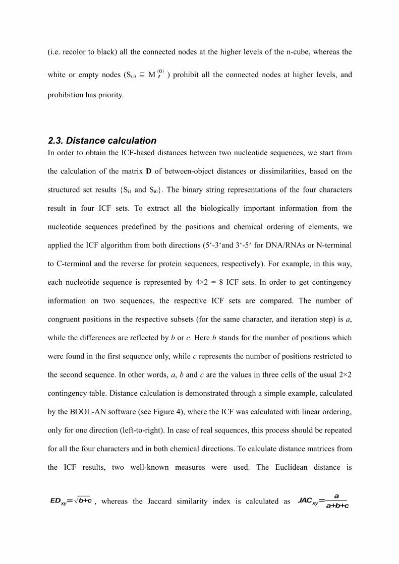
Fig. 4. Calculation of Jaccard and Euclidean distances between two binary strings: Encoding the positions for one type of nucleotide (e.g. adenine) of Sequences X and Y (a). The ICF subsets of the strings (b). Based on the cells of the 2×2 contingency table (c), a is the number of ICF subsets that are common in both ICF results, b is the number of ICF subsets that are characteristic for Sequence X exclusively and c is the number of ICF subsets that are characteristic for Sequence Y exclusively (d). From the a, b and c values of the ICF subsets Euclidean (EDxy) and Jaccard (JACDxy) distances (e) were calculated (see text, for formulae).
Fig. 5. Trees derived from the original sequences of 12 mammals (Penny et al., 1991) (a-c) and from the randomized versions (d-e).
Fig. 6. Principal Coordinates Analysis of 12 mammals (Penny et al. 1991) based on the distance matrix of Table 1.
Fig. 7. Guanine (G) and thymine (T) ICF graphs derived for 3 mammalian sequences by using the combined dataset (Penny et al. 1991). (BOOL-AN settings: partial ordering, starting position: 1, bidirectional ordering)
Tab.1
a) ICF + Jaccard distanceKangaroo: 0.0 - - - - - - - - - - -Monkey : 0.6887 0.0 - - - - - - - - - -Sheep : 0.7264 0.7421 0.0 - - - - - - - - -Horse : 0.6746 0.6635 0.6651 0.0 - - - - - - - -Rodent : 0.7174 0.6532 0.7637 0.6405 0.0 - - - - - - -Rabbit : 0.7088 0.6828 0.7367 0.6247 0.5988 0.0 - - - - - -Dog : 0.632 0.7166 0.769 0.652 0.6624 0.6523 0.0 - - - - -Pig : 0.6374 0.6359 0.5802 0.5141 0.626 0.6315 0.6516 0.0 - - - -Cat : 0.7051 0.7411 0.7953 0.7207 0.6454 0.7185 0.5651 0.6795 0.0 - - -Human : 0.7473 0.3862 0.7635 0.6956 0.6902 0.669 0.7366 0.6737 0.7779 0.0 - -Cow : 0.7377 0.7642 0.4652 0.6513 0.7511 0.7754 0.7796 0.6167 0.7424 0.7792 0.0 -Ape : 0.7708 0.4675 0.7747 0.7254 0.72 0.6989 0.7362 0.6983 0.7848 0.1636 0.7875 0.0
b) ICF + Euclidean distanceKangaroo: 0.0 - - - - - - - - - - -Monkey : 24.1661 0.0 - - - - - - - - - -Sheep : 25.1396 25.6125 0.0 - - - - - - - - -Horse : 23.8747 23.622 23.622 0.0 - - - - - - - -Rodent : 25.1396 23.4521 26.4197 23.1948 0.0 - - - - - - -Rabbit : 24.7184 24.0624 25.4755 22.6053 22.0227 0.0 - - - - - -Dog : 22.7376 25.04 26.4386 23.388 23.7697 23.3238 0.0 - - - - -Pig : 23.1948 23.1948 21.6795 20.0499 23.1084 23.0868 23.6854 0.0 - - - -Cat : 24.7386 25.7682 27.2397 25.2982 23.3666 25.1595 21.1424 24.4949 0.0 - - -Human : 26.1343 16.5831 26.5895 24.8395 24.7992 24.0416 25.9615 24.5561 27.1846 0.0 - -Cow : 25.3772 26.1534 18.2757 23.1948 26.0 26.4764 26.6646 22.5832 25.6905 26.9629 0.0 -Ape : 26.8887 18.7883 27.0 25.7488 25.7099 24.9399 26.0384 25.318 27.4773 10.2956 27.2947 0.0
Number of sequences
Length of sequences
10 100 1 00010 ~ 0 ~ 0.02 ~ 0.2
100 ~ 0.02 ~ 0.12 ~ 1.551 000 ~ 0.4 ~ 4 ~ 40
10 000 ~ 128 ~ 1 280 ~ 12 80020 000 ~ 817 ~ 8 170 ~ 81 700