36
Boosting for tumor Boosting for tumor classification classification with gene expression with gene expression data data Kfir Kfir Barhum Barhum
| Date post: | 22-Dec-2015 |
| Category: |
Documents |
| View: | 224 times |
| Download: | 2 times |
Boosting for tumor Boosting for tumor classification classification
with gene expression with gene expression datadata
Kfir Kfir BarhumBarhum
Overview – Today:Overview – Today:
Review the Classification ProblemReview the Classification ProblemFeatures (genes) PreselectionFeatures (genes) PreselectionWeak Learners & BoostingWeak Learners & BoostingLogitBoost AlgorithmLogitBoost AlgorithmReduction to the Binary CaseReduction to the Binary CaseErrors & ROC CurvesErrors & ROC CurvesSimulationSimulationResultsResults

Classification ProblemClassification Problem
Given n training data pairs:Given n training data pairs:
With : and With : and Corresponds to: X – features vector, p featuresCorresponds to: X – features vector, p features
Y – class labelY – class label
Typically: n between 20-80 samplesTypically: n between 20-80 samples
p varies from 2,000 to 20,000p varies from 2,000 to 20,000
nn yxyx ,,,, 11
pi Rx }1,...,0{ Jyi

Our Goal:Our Goal:
Construct a classifier C:Construct a classifier C:
From which a new tissue sample is classified From which a new tissue sample is classified based on it’s expression vector X. For the optimal based on it’s expression vector X. For the optimal C holds:C holds:
is minimalis minimal
We first handle only binary problems, for which:We first handle only binary problems, for which: Problem: p>>n Problem: p>>n
}1,...,0{)(: JXCXC
])(P[ YXC
}1,0{Y
we use boosting in conjunction with decision we use boosting in conjunction with decision trees !trees !

Features (genes) PreselectionFeatures (genes) Preselection
Problem: p>>n: sample size is much smaller than Problem: p>>n: sample size is much smaller than the features dimension (number of genes – p).the features dimension (number of genes – p).
Many genes are irrelevant for discrimination.Many genes are irrelevant for discrimination.
Optional solution:Optional solution: Dimensionality Reduction – was discussed earlierDimensionality Reduction – was discussed earlier
We score each individual gene g, with g {1,We score each individual gene g, with g {1,…,p}, according to it’s strength for phenotype …,p}, according to it’s strength for phenotype discrimination.discrimination.

Features (genes) PreselectionFeatures (genes) Preselection
We denote:We denote:
the expression value of gene g for individual Ithe expression value of gene g for individual I
Define:Define:
Which counts, for each input s.t. Y(x) = 0, the number of Which counts, for each input s.t. Y(x) = 0, the number of inputs of the form Y(x)=1, such that their expression inputs of the form Y(x)=1, such that their expression difference is negative. difference is negative.
)(gix
},...1{, 10 nNN Corresponding to set of indices having response Y( )=0, Y( )=1
ix ix
0 1
)()( 01)(
Ni Nixx gj
gi
gs

Features (genes) PreselectionFeatures (genes) Preselection
A gene does not discrimintate, if it’s score is about A gene does not discrimintate, if it’s score is about
It discriminates best when or even s(g) = It discriminates best when or even s(g) = 0 !0 !
Therefore defineTherefore define
We then simply take the genes with the highest values of q(g) as our top features.
Formal choice of can be done via cross-validation
0 1
)()( 01)(
Ni Nixx gj
gi
gs 1,0, iNn ii
2
10nn
1)( 0nngs
))(1),(max(:)( 0 gsnngsgq
pp ~
p~
Weak Learners & BoostingWeak Learners & Boosting
Suppose we had a “weak” learner, which can Suppose we had a “weak” learner, which can learn the data, and make a good estimation. learn the data, and make a good estimation.
Problem: Our learner has an error rate which is Problem: Our learner has an error rate which is too high for us.too high for us.
We search for a method to “boost” those weak We search for a method to “boost” those weak classifiers.classifiers.
Suppose…
Weak Learners & BoostingWeak Learners & Boosting
create an accurate combined classifier from a create an accurate combined classifier from a sequence of weak classifierssequence of weak classifiers
Weak classifiers are fitted to iteratively Weak classifiers are fitted to iteratively reweighedreweighed versions of the data.versions of the data.
In each boosting iteration In each boosting iteration mm, with m = 1…M:, with m = 1…M: Weight of data observations that have been Weight of data observations that have been
misclassified at the previous step, have their weights misclassified at the previous step, have their weights increasedincreased
The weight of data that has been classified correctly is The weight of data that has been classified correctly is decreaseddecreased
Introduce: …… Boosting !!!

Weak Learners & BoostingWeak Learners & Boosting
The The m m th weak classifier - - is forced to th weak classifier - - is forced to concentrate on the individual inputs that were concentrate on the individual inputs that were classified wrong at earlier iterations.classified wrong at earlier iterations.
Now, suppose we have remapped the output Now, suppose we have remapped the output classes Y(x) into {-1, 1} instead of {0,1}.classes Y(x) into {-1, 1} instead of {0,1}.
We have M different classifiers. How shall we We have M different classifiers. How shall we combine them into a stronger one ?combine them into a stronger one ?
)(mf

Weak Learners & BoostingWeak Learners & Boosting
Define the combined classifier to a weighted Define the combined classifier to a weighted majority vote of the “weak” classifiers:majority vote of the “weak” classifiers:
Points which need to be clarified, and specify the Points which need to be clarified, and specify the alg. :alg. : i) Which weak learners shall we use ? i) Which weak learners shall we use ?
ii) reweighing the data, and the aggregation weightsii) reweighing the data, and the aggregation weights
iii) How many iterations (choosing M) ?iii) How many iterations (choosing M) ?
“The Committee”
)()( )(
1
)( XfsignXC mM
mm
M

Weak Learners & BoostingWeak Learners & Boosting
Which type of “weak” learners: Which type of “weak” learners: Our case, we use a special kind of decision trees, Our case, we use a special kind of decision trees,
called stumps - trees with two terminal nodes. called stumps - trees with two terminal nodes.
Stumps are simple “rule of thumb”, which test Stumps are simple “rule of thumb”, which test on a single attribute.on a single attribute.
Our example:Our example:
7)26( ix
yes no
1iy 1iy
Weak Learners & BoostingWeak Learners & Boosting
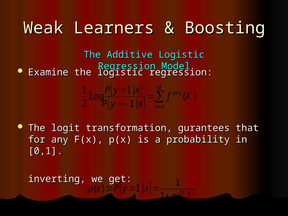
Examine the logistic regression:Examine the logistic regression:
The logit transformation, gurantees that for any The logit transformation, gurantees that for any F(x), p(x) is a probability in [0,1].F(x), p(x) is a probability in [0,1].
inverting, we get:inverting, we get:
M
m
m XfxyP
xyP
1
)( )(|1
|1log2
1
The Additive Logistic Regression The Additive Logistic Regression ModelModel
)(21
1|1:)(
xFexyPxp

LogitBoost AlgorithmLogitBoost Algorithm
So.. How to update the weights ?So.. How to update the weights ? We define a loss function, and follow gradient We define a loss function, and follow gradient
decent principle. decent principle.
AdaBoost uses the exponential loss function:AdaBoost uses the exponential loss function:
LogitBoost uses the binomial log-likelihood:LogitBoost uses the binomial log-likelihood:Let Let
DefineDefine
)()( xyFeEFJ
)))(1)(log(1())(log(:))(,( *** xpyxpyxpyl
)1log( )(2 xyFe
2/)1(* yy

LogitBoost AlgorithmLogitBoost Algorithm

LogitBoost AlgorithmLogitBoost Algorithm
Step 1: InitializationStep 1: Initialization
committee function:committee function:
initial probabilities:initial probabilities:
Step 2: LogitBoost iterationsStep 2: LogitBoost iterations
for m=1,2,...,M repeat:for m=1,2,...,M repeat:
0)()0( xF
21)()0( xp

LogitBoost AlgorithmLogitBoost Algorithm
A. Fitting the weak learnerA. Fitting the weak learner(i)(i) Compute working response and Compute working response and
weights for i=1,...,nweights for i=1,...,n
(ii)(ii) Fit a regression stump by weighted Fit a regression stump by weighted least squaresleast squares
)1( )1()1()( mmmi ppw
)(mf
)(
)1()( )(
mi
im
imi w
xpyz
n
ii
mi
mif
m xfzwf1
2)()()( ))((minarg
LogitBoost AlgorithmLogitBoost Algorithm
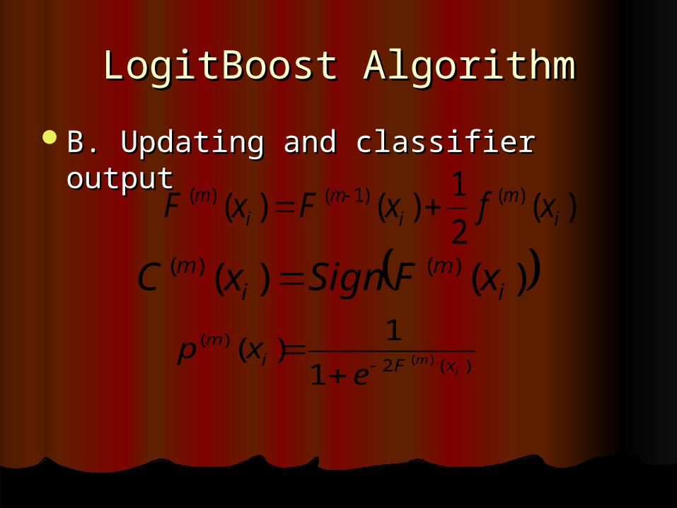
B. Updating and classifier outputB. Updating and classifier output
)(2
1)()( )()1()(
im
im
im xfxFxF
)(2
)()(
1
1)(
im xFi
m
exp
)()( )()(i
mi
m xFSignxC
LogitBoost AlgorithmLogitBoost Algorithm
Choosing the stop parameter M:Choosing the stop parameter M:
overfitting: when the model no longer overfitting: when the model no longer concentrates on the general aspects of the concentrates on the general aspects of the problem, but on specific it’s specific learnning setproblem, but on specific it’s specific learnning set
In general: Boosting is quite resistant to In general: Boosting is quite resistant to overfitting, so picking M higher as 100 will be overfitting, so picking M higher as 100 will be good enoughgood enough
Alternatively one can compute the binomial log-Alternatively one can compute the binomial log-likelihood for each iteration and choose to stop likelihood for each iteration and choose to stop on maximal approximationon maximal approximation
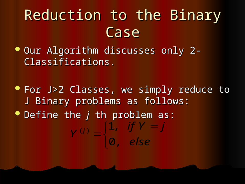
Reduction to the Binary CaseReduction to the Binary Case
Our Algorithm discusses only 2-Our Algorithm discusses only 2-Classifications. Classifications.
For J>2 Classes, we simply reduce to J For J>2 Classes, we simply reduce to J Binary problems as follows:Binary problems as follows:
Define the Define the jj th problem as: th problem as:
else
jYifY j
,0
,1)(

Reduction to the Binary CaseReduction to the Binary Case
Now we run J times the entire procedure, Now we run J times the entire procedure, including features preselection, and including features preselection, and estimating stopping parameter on new estimating stopping parameter on new data.data. different classes may preselect different different classes may preselect different
features (genes)features (genes)
This yields estimation probabilities:This yields estimation probabilities:
for j = 1,...,Jfor j = 1,...,J]|1[ˆ )( XYP j

Reduction to the Binary CaseReduction to the Binary Case
These can be converted into probability These can be converted into probability estimates for J=j via normalization:estimates for J=j via normalization:
Note that there exists a LogitBoost Note that there exists a LogitBoost Algorithm for J>2 classes, which treats the Algorithm for J>2 classes, which treats the multiclass problem simultaneously. It multiclass problem simultaneously. It yielded >1.5 times error rate.yielded >1.5 times error rate.
j
k
k
j
XYP
XYPXjYP
1
)(
)(
]|1[ˆ]|1[ˆ
]|[ˆ
Errors & ROC CurvesErrors & ROC Curves
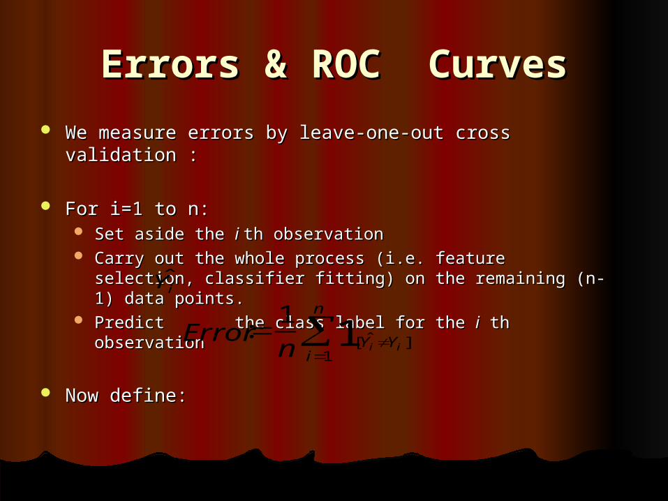
We measure errors by leave-one-out cross validation :We measure errors by leave-one-out cross validation :
For i=1 to n:For i=1 to n: Set aside the Set aside the i i th observationth observation Carry out the whole process (i.e. feature selection, classifier Carry out the whole process (i.e. feature selection, classifier
fitting) on the remaining (n-1) data points.fitting) on the remaining (n-1) data points. Predict the class label for the Predict the class label for the ii th observation th observation
Now define: Now define:
iY
n
iYY iin 1]ˆ[1
1:Error

Errors & ROC CurvesErrors & ROC Curves
False Positive Error -False Positive Error - when we classify a positive result as a negative onewhen we classify a positive result as a negative one
False Negative Error –False Negative Error – when we classify a negative result as a positive onewhen we classify a negative result as a positive one
Our Algorithm uses Equal misclassification Costs.Our Algorithm uses Equal misclassification Costs. (i.e. punish false-positive and false-negative errors (i.e. punish false-positive and false-negative errors
equally)equally)
QuestionQuestion: : Should this be the situationShould this be the situation ? ?
)1,0ˆ( ii YY
)0,1ˆ( ii YY

Recall Our Problem…Recall Our Problem…
NO !NO !
In our case: In our case: false positivefalse positive - means we diagnosed a normal - means we diagnosed a normal
tissue as a tumorous one. Probably further tissue as a tumorous one. Probably further tests will be carried out.tests will be carried out.
false negativefalse negative – We just classified a tumorous – We just classified a tumorous tissue as a healthy one. Outcome might be tissue as a healthy one. Outcome might be deadly.deadly.
Errors & ROC CurvesErrors & ROC Curves ROC Curves illustrate how accurate classifiers are under ROC Curves illustrate how accurate classifiers are under
asymmetricasymmetric losses losses
Each point corresponds to a specific probability which was Each point corresponds to a specific probability which was chosen as a threshold for positive classification.chosen as a threshold for positive classification.
Tradeoff between false positive and false negative errors.Tradeoff between false positive and false negative errors.
The closer the curve is to (0,1) on graph, the better the test.The closer the curve is to (0,1) on graph, the better the test.
ROC is: ROC is: Reciever Operating CharacteristicReciever Operating Characteristic – comes from field – comes from field called “Signal Detection Theory”, developed in WW-II, when called “Signal Detection Theory”, developed in WW-II, when radar had to decide whether a ship is friendly, enemy or just a radar had to decide whether a ship is friendly, enemy or just a backgroud noise.backgroud noise.

Errors & ROC CurvesErrors & ROC Curves
X-axis: negative examples X-axis: negative examples classified as positive classified as positive (tumorous ones)(tumorous ones)
Y-axis positive classified Y-axis positive classified correctlycorrectly
Each point on graph, Each point on graph, represents a Beta chosen represents a Beta chosen from [0,1] – as a threshold from [0,1] – as a threshold for positive classificationfor positive classification
Colon data w/o features Colon data w/o features preselectionpreselection
SimulationSimulation
The algorithm worked better than benchmark The algorithm worked better than benchmark methods for our real examination. methods for our real examination.
Real datasets are hard / expensive to getReal datasets are hard / expensive to get
Relevant differences between discrimination Relevant differences between discrimination methods might be difficult to detectmethods might be difficult to detect
Let’s try to simulate gene expression data, with Let’s try to simulate gene expression data, with large datasetlarge dataset

SimulationSimulation
Produce gene expression profiles from a Produce gene expression profiles from a multivariate normal distributionmultivariate normal distribution
where the covariance structure is from the colon where the covariance structure is from the colon datasetdataset
we took p = 2000 geneswe took p = 2000 genes Now assign one of two respond classes, with Now assign one of two respond classes, with
probabilities:probabilities:
,0~ pNX
))((~| xpBernoullixXY

SimulationSimulation
The conditional probabilities are take as follows:The conditional probabilities are take as follows: For j=1,...,10:For j=1,...,10:
Pick Cj of of size uniformly random from {1,...,10}Pick Cj of of size uniformly random from {1,...,10}
- - Mean values across random geneMean values across random gene
The expected number of relevant genes is therefore The expected number of relevant genes is therefore 10*5.5=5510*5.5=55
Pick from normal distrubtion with stddevPick from normal distrubtion with stddev 2,1,0.5 2,1,0.5
respectivelyrespectively
))((~| xpBernoullixXY
},...,1{ pC j
j
j
Cgj
gC
C
xx
)()(
jjj ,
)()(
1
)(11
)(1
)(log
jjj C
j
C
j
n
j
C
j xxxx
xp

SimulationSimulation
The trainning size was set to n=200 samples, The trainning size was set to n=200 samples, and tested on 1000 new observations testand tested on 1000 new observations test
The whole process was repeated 20 times, The whole process was repeated 20 times, and was tested against 2 well-known and was tested against 2 well-known benchmarks: 1-Nearest-Neighbor and benchmarks: 1-Nearest-Neighbor and Classification Tree.Classification Tree.
LogitBoost did better than both, even on LogitBoost did better than both, even on arbitrary fixed number of iterations (150)arbitrary fixed number of iterations (150)
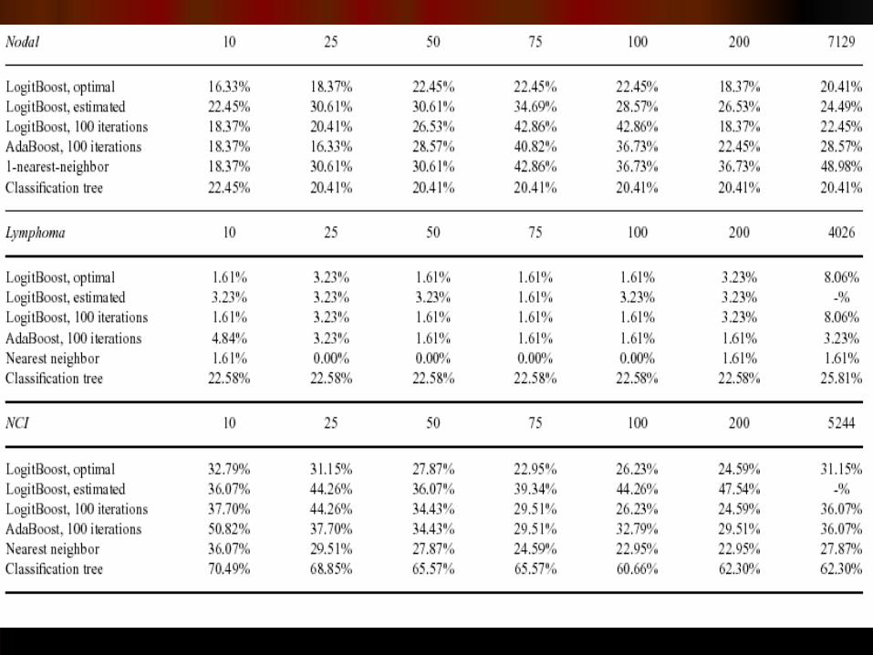
ResultsResults Boosting method was tried on 6 publicly avilable Boosting method was tried on 6 publicly avilable
datasets (Lukemia, Colon, Estrogen, Nodal, datasets (Lukemia, Colon, Estrogen, Nodal, Lymphoma, NCI).Lymphoma, NCI).
Data was processed and tested against other Data was processed and tested against other benchmarks: AdaBoost, 1-Nearest-Neighbor, benchmarks: AdaBoost, 1-Nearest-Neighbor, Classification Tree.Classification Tree.
On all 6 datasets the choice of the actual On all 6 datasets the choice of the actual stopping parameter did not matter, and the stopping parameter did not matter, and the choice of 100 iterations, did fairly well.choice of 100 iterations, did fairly well.

ResultsResults
Tests were made for several numbers of Tests were made for several numbers of preselected features, and all of them.preselected features, and all of them.
Using all genes, the classical method of 1-Using all genes, the classical method of 1-nearest-neighbor is interrupted by noise nearest-neighbor is interrupted by noise variables, and the boosting methods outperforms variables, and the boosting methods outperforms it.it.

ResultsResults

-fin-


![Delta Boosting Machine and its Application in Actuarial ... · (MARS), regression trees [22] and boosting. 1.1. The Boosting Algorithms. Boosting methods are based on an idea of com-bining](https://static.documents.pub/doc/80x56/5f39fd86e92ad51969114a8c/delta-boosting-machine-and-its-application-in-actuarial-mars-regression-trees.jpg)


