Boosting the Actor with Dual Critic * Bo Dai 1 , * Albert Shaw 1 , Niao He 2 , Lihong Li 3 , Le Song 1 1 Georgia Institute of Technology {bodai, ashaw596}@gatech.edu, [email protected]2 University of Illinois at Urbana-Champaign [email protected]3 Google AI [email protected]January 1, 2018 Abstract This paper proposes a new actor-critic-style algorithm called Dual Actor-Criticor Dual-AC. It is derived in a principled way from the Lagrangian dual form of the Bellman optimality equation, which can be viewed as a two-player game between the actor and a critic-like function, which is named as dual critic. Compared to its actor-critic relatives, Dual-AC has the desired property that the actor and dual critic are updated cooperatively to optimize the same objective function, providing a more transparent way for learning the critic that is directly related to the objective function of the actor. We then provide a concrete algorithm that can effectively solve the minimax optimization problem, using techniques of multi-step bootstrapping, path regularization, and stochastic dual ascent algorithm. We demonstrate that the proposed algorithm achieves the state-of-the-art performances across several benchmarks. 1 Introduction Reinforcement learning (RL) algorithms aim to learn a policy that maximizes the long-term return by sequentially interacting with an unknown environment. Value-function-based algorithms first approximate the optimal value function, which can then be used to derive a good policy. These methods (Sutton, 1988; Watkins, 1989) often take advantage of the Bellman equation and use bootstrapping to make learning more sample efficient than Monte Carlo estimation (Sutton and Barto, 1998). However, the relation between the quality of the learned value function and the quality of the derived policy is fairly weak (Bertsekas and Tsitsiklis, 1996). Policy-search-based algorithms such as REINFORCE (Williams, 1992) and others (Kakade, 2002; Schulman et al., 2015a), on the other hand, assume a fixed space of parameterized policies and search for the optimal policy parameter based on unbiased Monte Carlo estimates. The parameters are often updated incrementally along stochastic directions that on average are guaranteed to increase the policy quality. Unfortunately, they often have a greater variance that results in a higher sample complexity. Actor-critic methods combine the benefits of these two classes, and have proved successful in a number of challenging problems such as robotics (Deisenroth et al., 2013), meta-learning (Bello et al., 2016), and games (Mnih et al., 2016). An actor-critic algorithm has two components: the actor (policy) and the critic (value function). As in policy-search methods, actor is updated towards the direction of policy improvement. However, the update directions are computed with the help of the critic, which can be more efficiently learned as in value-function-based methods (Sutton et al., 2000; Konda and Tsitsiklis, 2003; Peters et al., 2005; * The first two authors equally contributed. 1 arXiv:1712.10282v1 [cs.LG] 29 Dec 2017
Transcript
Boosting the Actor with Dual Critic∗Bo Dai1, ∗Albert Shaw1, Niao He2, Lihong Li3, Le Song1
This paper proposes a new actor-critic-style algorithm called Dual Actor-Criticor Dual-AC. It isderived in a principled way from the Lagrangian dual form of the Bellman optimality equation, whichcan be viewed as a two-player game between the actor and a critic-like function, which is named as dualcritic. Compared to its actor-critic relatives, Dual-AC has the desired property that the actor and dualcritic are updated cooperatively to optimize the same objective function, providing a more transparentway for learning the critic that is directly related to the objective function of the actor. We then providea concrete algorithm that can effectively solve the minimax optimization problem, using techniques ofmulti-step bootstrapping, path regularization, and stochastic dual ascent algorithm. We demonstratethat the proposed algorithm achieves the state-of-the-art performances across several benchmarks.
1 Introduction
Reinforcement learning (RL) algorithms aim to learn a policy that maximizes the long-term return bysequentially interacting with an unknown environment. Value-function-based algorithms first approximatethe optimal value function, which can then be used to derive a good policy. These methods (Sutton, 1988;Watkins, 1989) often take advantage of the Bellman equation and use bootstrapping to make learning moresample efficient than Monte Carlo estimation (Sutton and Barto, 1998). However, the relation between thequality of the learned value function and the quality of the derived policy is fairly weak (Bertsekas andTsitsiklis, 1996). Policy-search-based algorithms such as REINFORCE (Williams, 1992) and others (Kakade,2002; Schulman et al., 2015a), on the other hand, assume a fixed space of parameterized policies and searchfor the optimal policy parameter based on unbiased Monte Carlo estimates. The parameters are oftenupdated incrementally along stochastic directions that on average are guaranteed to increase the policyquality. Unfortunately, they often have a greater variance that results in a higher sample complexity.
Actor-critic methods combine the benefits of these two classes, and have proved successful in a numberof challenging problems such as robotics (Deisenroth et al., 2013), meta-learning (Bello et al., 2016), andgames (Mnih et al., 2016). An actor-critic algorithm has two components: the actor (policy) and the critic(value function). As in policy-search methods, actor is updated towards the direction of policy improvement.However, the update directions are computed with the help of the critic, which can be more efficiently learnedas in value-function-based methods (Sutton et al., 2000; Konda and Tsitsiklis, 2003; Peters et al., 2005;
∗The first two authors equally contributed.
1
arX
iv:1
712.
1028
2v1
[cs
.LG
] 2
9 D
ec 2
017
Bhatnagar et al., 2009; Schulman et al., 2015b). Although the use of a critic may introduce bias in learningthe actor, its reduces variance and thus the sample complexity as well, compared to pure policy-searchalgorithms.
While the use of a critic is important for the efficiency of actor-critic algorithms, it is not entirely clearhow the critic should be optimized to facilitate improvement of the actor. For some parametric family ofpolicies, it is known that a certain compatibility condition ensures the actor parameter update is an unbiasedestimate of the true policy gradient (Sutton et al., 2000). In practice, temporal-difference methods areperhaps the most popular choice to learn the critic, especially when nonlinear function approximation is used(e.g., Schulman et al. (2015b)).
In this paper, we propose a new actor-critic-style algorithm where the actor and the critic-like function,which we named as dual critic, are trained cooperatively to optimize the same objective function. Thealgorithm, called Dual Actor-Critic, is derived in a principled way by solving a dual form of the Bellmanequation (Bertsekas and Tsitsiklis, 1996). The algorithm can be viewed as a two-player game between theactor and the dual critic, and in principle can be solved by standard optimization algorithms like stochasticgradient descent (Section 2). We emphasize the dual critic is not fitting the value function for current policy,but that of the optimal policy. We then show that, when function approximation is used, direct application ofstandard optimization techniques can result in instability in training, because of the lack of convex-concavityin the objective function (Section 3). Inspired by the augmented Lagrangian method (Luenberger and Ye,2015; Boyd et al., 2010), we propose path regularization for enhanced numerical stability. We also generalizethe two-player game formulation to the multi-step case to yield a better bias/variance tradeoff. The fullalgorithm is derived and described in Section 4, and is compared to existing algorithms in Section 5. Finally,our algorithm is evaluated on several locomotion tasks in the MuJoCo benchmark (Todorov et al., 2012), andcompares favorably to state-of-the-art algorithms across the board.
Notation. We denote a discounted MDP by M = (S,A, P,R, γ), where S is the state space, A the actionspace, P (·|s, a) the transition probability kernel defining the distribution over next-state upon taking actiona in state x, R(s, a) the corresponding immediate rewards, and γ ∈ (0, 1) the discount factor. If there is noambiguity, we will use
∑a f(a) and
∫f(a)da interchangeably.
2 Duality of Bellman Optimality Equation
In this section, we first describe the linear programming formula of the Bellman optimality equation (Bertsekaset al., 1995; Puterman, 2014), paving the path for a duality view of reinforcement learning via Lagrangianduality. In the main text, we focus on MDPs with finite state and action spaces for simplicity of exposition.We extend the duality view to continuous state and action spaces in Appendix A.2.
Given an initial state distribution µ(s), the reinforcement learning problem aims to find a policy π(·|s) :S → P(A) that maximizes the total expected discounted reward with P(A) denoting all the probabilitymeasures over A, i.e.,
Es0∼µ(s)Eπ[∑∞
i=0 γiR(si, ai)
], (1)
where si+1 ∼ P (·|si, ai), ai ∼ π(·|si).Define V ∗(s) := maxπ∈P(A) E
[∑∞i=0 γ
iR(si, ai)|s0 = s], the Bellman optimality equation states that:
V ∗(s) = (T V ∗)(s) := maxa∈A
R(s, a) + γEs′|s,a [V ∗(s′)]
, (2)
which can be formulated as a linear program (Puterman, 2014; Bertsekas et al., 1995):
P∗ := minV
(1− γ)Es∼µ(s) [V (s)] (3)
s.t. V (s) > R(s, a) + γEs′|s,a [V (s′)] , ∀(s, a) ∈ S ×A.
For completeness, we provide the derivation of the above equivalence in Appendix A. Without loss of generality,we assume there exists an optimal policy for the given MDP, namely, the linear programming is solvable.
2
The optimal policy can be obtained from the solution to the linear program (3) via
π∗(s) = argmaxa∈A
R(s, a) + γEs′|s,a [V ∗(s′)]
. (4)
The dual form of the LP below is often easier to solve and yield more direct relations to the optimal policy.
D∗ := maxρ>0
∑(s,a)∈S×A
R(s, a)ρ(s, a) (5)
s.t.∑a∈A ρ(s′, a) = (1− γ)µ(s′) + γ
∑s,a∈S×A ρ(s, a)P (s′|s, a)ds,∀s′ ∈ S.
Since the primal LP is solvable, the dual LP is also solvable, and P∗ − D∗ = 0. The optimal dual variablesρ∗(s, a) and optimal policy π∗(a|s) are closely related in the following manner:
Theorem 1 (Policy from dual variables)∑s,a∈S×A ρ
∗(s, a) = 1, and π∗(a|s) = ρ∗(s,a)∑a∈A ρ
∗(s,a) .
Since the goal of reinforcement learning task is to learn an optimal policy, it is appealing to deal with theLagrangian dual which optimizes the policy directly, or its equivalent saddle point problem that jointly learnsthe optimal policy and value function.
Theorem 2 (Competition in one-step setting) The optimal policy π∗, actor, and its correspondingvalue function V ∗, dual critic, is the solution to the following saddle-point problem
maxα∈P(S),π∈P(A)
minV
L(V, α, π) := (1− γ)Es∼µ(s) [V (s)] +∑
(s,a)∈S×A
α(s)π (a|s) ∆[V ](s, a), (6)
where ∆[V ](s, a) := R(s, a) + γEs′|s,a[V (s′)]− V (s).
The saddle point optimization (6) provides a game perspective in understanding the reinforcement learningproblem (Goodfellow et al., 2014). The learning procedure can be thought as a game between the dual critic,i.e., value function for optimal policy, and the weighted actor, i.e., α(s)π(a|s): the dual critic V seeks thevalue function to satisfy the Bellman equation, while the actor π tries to generate state-action pairs thatbreak the satisfaction. Such a competition introduces new roles for the actor and the dual critic, and moreimportantly, bypasses the unnecessary separation of policy evaluation and policy improvement proceduresneeded in a traditional actor-critic framework.
3 Sources of Instability
To solve the dual problem in (6), a straightforward idea is to apply stochastic mirror prox (Nemirovskiet al., 2009) or stochastic primal-dual algorithm (Chen et al., 2014) to address the saddle point problemin (6). Unfortunately, such algorithms have limited use beyond special cases. For example, for an MDPwith finite state and action spaces, the one-step saddle-point problem (6) with tabular parametrization isconvex-concave, and finite-sample convergence rates can be established; see e.g., Chen and Wang (2016) andWang (2017). However, when the state/action spaces are large or continuous so that function approximationmust be used, such convergence guarantees no longer hold due to lack of convex-concavity. Consequently,directly solving (6) can suffer from severe bias and numerical issues, resulting in poor performance in practice(see, e.g., Figure 1):
1. Large bias in one-step Bellman operator: It is well-known that one-step bootstrapping in temporaldifference algorithms has lower variance than Monte Carlo methods and often require much fewersamples to learn. But it produces biased estimates, especially when function approximation is used.Such a bias is especially troublesome in our case as it introduces substantial noise in the gradients toupdate the policy parameters.
3
2. Absence of local convexity and duality: Using nonlinear parametrization will easily break thelocal convexity and duality between the original LP and the saddle point problem, which are known asthe necessary conditions for the success of applying primal-dual algorithm to constrained problems (Lu-enberger and Ye, 2015). Thus none of the existing primal-dual type algorithms will remain stable andconvergent when directly optimizing the saddle point problem without local convexity.
3. Biased stochastic gradient estimator with under-fitted value function: In the absence of localconvexity, the stochastic gradient w.r.t. the policy π constructed from under-fitted value functionwill presumably be biased and futile to provide any meaningful improvement of the policy. Hence,naively extending the stochastic primal-dual algorithms in Chen and Wang (2016); Wang (2017) for theparametrized Lagrangian dual, will also lead to biased estimators and sample inefficiency.
4 Dual Actor-Critic
In this section, we will introduce several techniques to bypass the three instability issues in the previoussection: (1) generalization of the minimax game to the multi-step case to achieve a better bias-variancetradeoff; (2) use of path regularization in the objective function to promote local convexity and duality; and(3) use of stochastic dual ascent to ensure unbiased gradient estimates.
4.1 Competition in multi-step setting
In this subsection, we will extend the minimax game between the actor and critic to the multi-step setting,which has been widely utilized in temporal-difference algorithms for better bias/variance tradeoffs (Suttonand Barto, 1998; Kearns and Singh, 2000). By the definition of the optimal value function, it is easy to derivethe k-step Bellman optimality equation as
V ∗(s) =(T kV ∗
)(s) := maxπ∈P
Eπ[∑k
i=0 γiR(si, ai)
]+ γk+1Eπ [V ∗(sk+1)]
. (7)
Similar to the one-step case, we can reformulate the multi-step Bellman optimality equation into a formsimilar to the LP formulation, and then we establish the duality, which leads to the following mimimaxproblem:
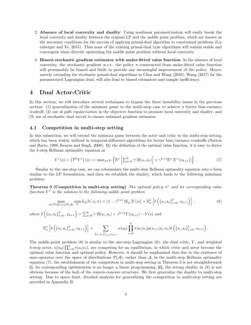
Theorem 3 (Competition in multi-step setting) The optimal policy π∗ and its corresponding valuefunction V ∗ is the solution to the following saddle point problem
The saddle-point problem (8) is similar to the one-step Lagrangian (6): the dual critic, V , and weighted
k-step actor, α(s0)∏ki=0 π(ai|si), are competing for an equilibrium, in which critic and actor become the
optimal value function and optimal policy. However, it should be emphasized that due to the existence ofmax-operator over the space of distributions P(A), rather than A, in the multi-step Bellman optimalityequation (7), the establishment of the competition in multi-step setting in Theorem 3 is not straightforward:i), its corresponding optimization is no longer a linear programming; ii), the strong duality in (8) is notobvious because of the lack of the convex-concave structure. We first generalize the duality to multi-stepsetting. Due to space limit, detailed analyses for generalizing the competition to multi-step setting areprovided in Appendix B.
4
4.2 Path Regularization
When function approximation is used, the one-step or multi-step saddle point problems (8) will no longer beconvex in the primal parameter space. This could lead to severe instability and even divergence when solved bybrute-force stochastic primal-dual algorithms. One then desires to partially convexify the objectives withoutaffecting the optimal solutions. The augmented Lagrangian method (Boyd et al., 2010; Luenberger and Ye,2015), also known as method of multipliers, is designed and widely used for such purposes. However, directlyapplying this method would require introducing penalty functions of the multi-step Bellman operator, whichrenders extra complexity and challenges in optimization. Interested readers are referred to Appendix B.2 fordetails.
Instead, we propose to use path regularization, as a stepping stone for promoting local convexity andcomputation efficiency. The regularization term is motivated by the fact that the optimal value functionsatisfies the constraint V (s) = Eπ∗
[∑∞i=0 γ
iR(si, ai)|s]. In the same spirit as augmented Lagrangian, we will
introduce to the objective the simple penalty function Es∼µ(s)[(Eπb
Note that in the penalty function we use some behavior policy πb instead of the optimal policy, sincethe latter is unavailable. Adding such a regularization enables local duality in the primal parameter space.Indeed, this can be easily verified by showing the positive definite of the Hessian at a local solution. We namethe regularization as path regularization, since it exploits the rewards in the sample path to regularize thesolution path of value function V in the optimization procedure. As a by-product, the regularization alsoprovides the mechanism to utilize off-policy samples from behavior policy πb.
One can also see that the regularization indeed provides guidance and preference to search for the solutionpath. Specifically, in the learning procedure of V , each update towards to the optimal value function whilearound the value function of the behavior policy πb. Intuitively, such regularization restricts the feasibledomain of the candidates V to be a ball centered at V πb . Besides enhancing the local convexity, such penaltyalso avoid unbounded V in learning procedure which makes the optimization invalid, and thus more numericalrobust. As long as the optimal value function is indeed in such region, there will be no side-effect introduced.Formally, we can show that with appropriate ηV , the optimal solution (V ∗, α∗, π∗) is not affected. The mainresults of this subsection are summarized by the following theorem.
Theorem 4 (Property of path regularization) The local duality holds for Lr(V, α, π). Denote (V ∗, α∗, π∗)as the solution to Bellman optimality equation, with some appropriate ηV ,
(V ∗, α∗, π∗) = argmaxα∈P(S),π∈P(A)
argminV
Lr(V, α, π).
The proof of the theorem is given in Appendix B.3. We emphasize that the theorem holds when V is givenenough capacity, i.e., in the nonparametric limit. With parametrization introduced, definitely approximationerror will be introduced, and the valid range of ηV , which keeps optimal solution unchanged, will be affected.However, the function approximation error is still an open problem for general class of parametrization, weomit such discussion here which is out of the range of this paper.
4.3 Stochastic Dual Ascent Update
Rather than the primal form, i.e., minV maxα∈P(S),π∈P(A) Lr(V, α, π), we focus on optimizing the dualform maxα∈P(S),π∈P(A) minV Lr(V, α, π). The major reason is due to the sample efficiency consideration.In the primal form, to apply the stochastic gradient descent algorithm at V t, one need to solve themaxα∈P(S),π∈P(A) Lr(V
t, α, π) which involves sampling from each π and α during the solution path for thesubproblem. We define the regularized dual function `r(α, π) := minV Lr(V, α, π). We first show the unbiased
5
gradient estimator of `r w.r.t. θρ = (θα, θπ), which are parameters associated with α and π. Then, weincorporate the stochastic update rule to dual ascent algorithm (Boyd et al., 2010), resulting in the dualactor-critic (Dual-AC) algorithm.
The gradient estimators of the dual functions can be derived using chain rule and are provided below.
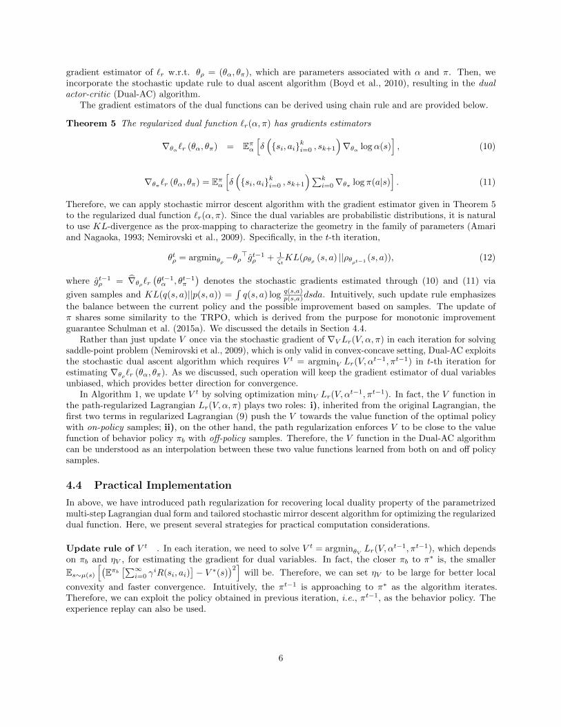
Theorem 5 The regularized dual function `r(α, π) has gradients estimators
∇θα`r (θα, θπ) = Eπα[δ(si, aiki=0 , sk+1
)∇θα logα(s)
], (10)
∇θπ`r (θα, θπ) = Eπα[δ(si, aiki=0 , sk+1
)∑ki=0∇θπ log π(a|s)
]. (11)
Therefore, we can apply stochastic mirror descent algorithm with the gradient estimator given in Theorem 5to the regularized dual function `r(α, π). Since the dual variables are probabilistic distributions, it is naturalto use KL-divergence as the prox-mapping to characterize the geometry in the family of parameters (Amariand Nagaoka, 1993; Nemirovski et al., 2009). Specifically, in the t-th iteration,
θtρ = argminθρ −θρ>gt−1ρ + 1
ζtKL(ρθρ (s, a) ||ρθρt−1 (s, a)), (12)
where gt−1ρ = ∇θρ`r(θt−1α , θt−1π
)denotes the stochastic gradients estimated through (10) and (11) via
given samples and KL(q(s, a)||p(s, a)) =∫q(s, a) log q(s,a)
p(s,a)dsda. Intuitively, such update rule emphasizes
the balance between the current policy and the possible improvement based on samples. The update ofπ shares some similarity to the TRPO, which is derived from the purpose for monotonic improvementguarantee Schulman et al. (2015a). We discussed the details in Section 4.4.
Rather than just update V once via the stochastic gradient of ∇V Lr(V, α, π) in each iteration for solvingsaddle-point problem (Nemirovski et al., 2009), which is only valid in convex-concave setting, Dual-AC exploitsthe stochastic dual ascent algorithm which requires V t = argminV Lr(V, α
t−1, πt−1) in t-th iteration forestimating ∇θρ`r (θα, θπ). As we discussed, such operation will keep the gradient estimator of dual variablesunbiased, which provides better direction for convergence.
In Algorithm 1, we update V t by solving optimization minV Lr(V, αt−1, πt−1). In fact, the V function in
the path-regularized Lagrangian Lr(V, α, π) plays two roles: i), inherited from the original Lagrangian, thefirst two terms in regularized Lagrangian (9) push the V towards the value function of the optimal policywith on-policy samples; ii), on the other hand, the path regularization enforces V to be close to the valuefunction of behavior policy πb with off-policy samples. Therefore, the V function in the Dual-AC algorithmcan be understood as an interpolation between these two value functions learned from both on and off policysamples.
4.4 Practical Implementation
In above, we have introduced path regularization for recovering local duality property of the parametrizedmulti-step Lagrangian dual form and tailored stochastic mirror descent algorithm for optimizing the regularizeddual function. Here, we present several strategies for practical computation considerations.
Update rule of V t . In each iteration, we need to solve V t = argminθV Lr(V, αt−1, πt−1), which depends
on πb and ηV , for estimating the gradient for dual variables. In fact, the closer πb to π∗ is, the smaller
Es∼µ(s)[(Eπb
[∑∞i=0 γ
iR(si, ai)]− V ∗(s)
)2]will be. Therefore, we can set ηV to be large for better local
convexity and faster convergence. Intuitively, the πt−1 is approaching to π∗ as the algorithm iterates.Therefore, we can exploit the policy obtained in previous iteration, i.e., πt−1, as the behavior policy. Theexperience replay can also be used.
6
Algorithm 1 Dual Actor-Critic (Dual-AC)
1: Initialize θ0V , θ0αand θ0π randomly, set β ∈ [ 12 , 1].2: for episode t = 1, . . . , T do3: Start from s ∼ αt−1(s), collect samples τlml=1 follows behavior policy πt−1.
4: Update θtV = argminθV Lr(V, αt−1, πt−1) by SGD based on τlml=1.
5: Update αt(s) according to closed-form (14).6: Decay the stepsize ζt in rate C
n0+1/tβ.
7: Compute the stochastic gradients for θπ following (11).8: Update θtπ according to the exact prox-mapping (16) or the approximate closed-form (17).9: end for
Furthermore, notice the L(V, αt−1, πt−1) is a expectation of functions of V , we will use stochastic gradientdescent algorithm for the subproblem. Other efficient optimization algorithms can be used too. Specifically,the unbiased gradient estimator for ∇θV L(V, αt−1, πt−1) is
We can use k-step Monte Carlo approximation for Eπbµ[∑∞
i=0 γiR(si, ai)
]in the gradient estimator. As
k is large enough, the truncate error is negligible (Sutton and Barto, 1998). We will iterate via θt,iV =
θt,i−1V + κi∇θt,i−1V
Lr(V, αt−1, πt−1) until the algorithm converges.
It should be emphasized that in our algorithm, V t is not the estimation of the value function of πt.Although V t eventually becomes the estimation of the optimal value function once the algorithm achieves theglobal optimum, in each update, the V t is one function which helps the current policy to be improved. Fromthis perspective, the Dual-AC bypasses the policy evaluation step.
Update rule of αt . In practice, we may face with the situation that the initial sampling distribution isfixed, e.g., in MuJoCo tasks. Therefore, we cannot obtain samples from αt(s) at each iteration. We assumethat ∃ηµ ∈ (0, 1], such that α(s) = (1− ηµ)β(s) + ηµµ(s) with β(s) ∈ P(S). Hence, we have
Eπα[δ(si, aiki=0 , sk+1
)]= Eπµ
[(α(s) + ηµ) δ
(si, aiki=0 , sk+1
)]where α(s) = (1− ηµ)β(s)µ(s) . Note that such an assumption is much weaker comparing with the requirement
for popular policy gradient algorithms (e.g., Sutton et al. (1999); Silver et al. (2014)) that assumes µ(s) to bea stationary distribution. In fact, we can obtain a closed-form update for α if a square-norm regularizationterm is introduced into the dual function. Specifically,
Theorem 6 In t-th iteration, given V t and πt−1,
argmaxα>0
Eµ(s)πt−1(s)
[(α(s) + ηµ) δ
(si, aiki=0 , sk+1
)]− ηα ‖α‖2µ (14)
=1
ηαmax
(0,Eπ
t−1[δ(si, aiki=0 , sk+1
)]). (15)
Then, we can update αt through (14) with Monte Carlo approximation of Eπt−1[δ(si, aiki=0 , sk+1
)],
avoiding the parametrization of α. As we can see, the αt(s) reweights the samples based on the temporaldifferences and this offers a principled justification for the heuristic prioritized reweighting trick used in (Schaulet al., 2015).
7
Update rule of θtπ . The parameters for dual function, θρ, are updated by the prox-mapping operator (12)following the stochastic mirror descent algorithm for the regularized dual function. Specifically, in t-thiteration, given V t and αt, for θπ, the prox-mapping (12) reduces to
θtπ = argminθπ −θπ>gtπ + 1
ζtKL
(πθπ (a|s)||πθt−1
π(a|s)
), (16)
where gtπ = ∇θπ`r (θtα, θtπ). Then, the update rule will become exactly the natural policy gradient (Kakade,
2002) with a principled way to compute the “policy gradient” gtπ. This can be understood as the penaltyversion of the trust region policy optimization (Schulman et al., 2015a), in which the policy parametersconservative update in terms of KL-divergence is achieved by adding explicit constraints.
Exactly solving the prox-mapping for θπ requires another optimization, which may be expensive. To furtheraccelerate the prox-mapping, we approximate the KL-divergence with the second-order Taylor expansion,and obtain an approximate closed-form update given by
θtπ ≈ argminθπ
−θπ>gtπ +
1
2
∥∥θπ − θt−1π
∥∥2Ft
= θt−1π + ζtF
−1t gtπ (17)
where Ft := Eαtπt−1
[∇2 log πθt−1
π
]denotes the Fisher information matrix. Empirically, we may normalize
the gradient by its norm√gtπF
−1t gtπ (Rajeswaran et al., 2017) for better performances.
Combining these practical tricks to the stochastic mirror descent update eventually gives rise to the dualactor-criticalgorithm outlined in Algorithm 1.
5 Related Work
The dual actor-criticalgorithm includes both the learning of optimal value function and optimal policy in aunified framework based on the duality of the linear programming (LP) representation of Bellman optimalityequation. The linear programming representation of Bellman optimality equation and its duality have beenutilized for (approximate) planning problem (de Farias and Roy, 2004; Wang et al., 2008; Pazis and Parr, 2011;O’Donoghue et al., 2011; Malek et al., 2014; Cogill, 2015), in which the transition probability of the MDP isknown and the value function or policy are in tabular form. Chen and Wang (2016); Wang (2017) applystochastic first-order algorithms (Nemirovski et al., 2009) for the one-step Lagrangian of the LP problem inreinforcement learning setting. However, as we discussed in Section 3, their algorithm is restricted to tabularparametrization and are not applicable to MDPs with large or continuous state/action spaces.
The duality view has also been exploited in Neu et al. (2017). Their algorithm is based on the duality ofentropy-regularized Bellman equation (Todorov, 2007; Rubin et al., 2012; Fox et al., 2015; Haarnoja et al.,2017; Nachum et al., 2017), rather than the exact Bellman optimality equation used in our work. Meanwhile,their algorithm is only derived and tested in tabular form.
Our dual actor-criticalgorithm can be understood as a nontrivial extension of the (approximate) dualgradient method (Bertsekas, 1999, Chapter 6.3) using stochastic gradient and Bregman divergence, whichessentially parallels the view of (approximate) stochastic mirror descent algorithm (Nemirovski et al., 2009)in the primal space. As a result, the algorithm converges with diminishing stepsizes and decaying errors fromsolving subproblems.
Particularly, the update rules of α and π in the dual actor-criticare related to several existing algorithms.As we see in the update of α, the algorithm reweighs the samples which are not fitted well. This is related tothe heuristic prioritized experience replay (Schaul et al., 2015). For the update in π, the proposed algorithmbears some similarities with trust region poicy gradient (TRPO) (Schulman et al., 2015a) and natural policygradient (Kakade, 2002; Rajeswaran et al., 2017). Indeed, TRPO and NPR solve the same prox-mappingbut are derived from different perspectives. We emphasize that although the updating rules share someresemblance to several reinforcement learning algorithms in the literature, they are purely originated from astochastic dual ascent algorithm for solving the two-play game derived from Bellman optimality equation.
Figure 1: Comparison between the Dual-AC and its variants for justifying the analysis of the source ofinstability.
6 Experiments
We evaluated the dual actor-critic (Dual-AC) algorithm on several continuous control environments fromthe OpenAI Gym (Brockman et al., 2016) with MuJoCo physics simulator (Todorov et al., 2012). Wecompared Dual-AC with several representative actor-critic algorithms, including trust region policy optimiza-tion (TRPO) (Schulman et al., 2015a) and proximal policy optimization (PPO) (Schulman et al., 2017)1.We ran the algorithms with 5 random seeds and reported the average rewards with 50% confidence interval.Details of the tasks and setups of these experiments including the policy/value function architectures and thehyperparameters values, are provided in Appendix C.
6.1 Ablation Study
To justify our analysis in identifying the sources of instability in directly optimizing the parametrizedone-step Lagrangian duality and the effect of the corresponding components in the dual actor-criticalgorithm,we perform comprehensive Ablation study in InvertedDoublePendulum-v1, Swimmer-v1, and Hopper-v1environments. We also considered the effect of k = 10, 50 besides the one-step result in the study todemonstrate the benefits of multi-step.
We conducted comparison between the Dual-AC and its variants, including Dual-AC w/o multi-step,Dual-AC w/o path-regularization, Dual-AC w/o unbiased V , and the naive Dual-AC, for demonstrating thethree instability sources in Section 3, respectively, as well as varying the k = 10, 50 in Dual-AC. Specifically,Dual-AC w/o path-regularization removes the path-regularization components; Dual-AC w/o multi-stepremoves the multi-step extension and the path-regularization; Dual-AC w/o unbiased V calculates thestochastic gradient without achieving the convergence of inner optimization on V ; and the naive Dual-AC isthe one without all components. Moreover, Dual-AC with k = 10 and Dual-AC with k = 50 denote thelength of steps set to be 10 and 50, respectively.
The empirical performances on InvertedDoublePendulum-v1, Swimmer-v1, and Hopper-v1 tasks are shownin Figure 1. The results are consistent across the tasks with the analysis. The naive Dual-AC performs theworst. The performances of the Dual-AC found the optimal policy which solves the problem much fasterthan the alternative variants. The Dual-AC w/o unbiased V converges slower, showing its sample inefficiencycaused by the bias in gradient calculation. The Dual-AC w/o multi-step and Dual-AC w/o path-regularizationcannot converge to the optimal policy, indicating the importance of the path-regularization in recoveringthe local duality. Meanwhile, the performance of Dual-AC w/o multi-step is worse than Dual-AC w/o path-regularization, showing the bias in one-step can be alleviated via multi-step trajectories. The performances ofDual-AC become better with the length of step k increasing on these three tasks. We conjecture that the
1As discussed in Henderson et al. (2017), different implementations of TRPO and PPO can provide different performances.For a fair comparison, we use the codes from https://github.com/joschu/modular rl reported to have achieved the best scoresin Henderson et al. (2017).
9
main reason may be that in these three MuJoCo environments, the bias dominates the variance. Therefore,with the k increasing, the proposed Dual-AC obtains more accumulate rewards.
6.2 Comparison in Continuous Control Tasks
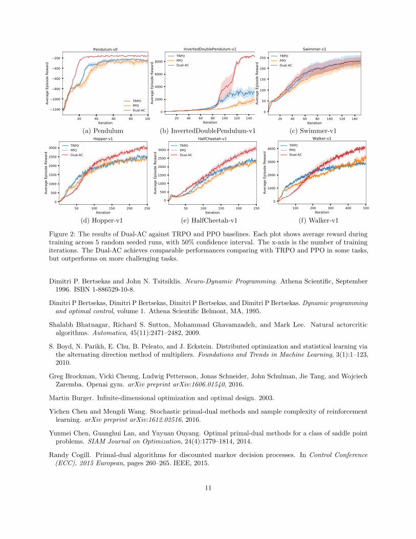
In this section, we evaluated the Dual-AC against TRPO and PPO across multiple tasks, including theInvertedDoublePendulum-v1, Hopper-v1, HalfCheetah-v1, Swimmer-v1 and Walker-v1. These tasks havedifferent dynamic properties, ranging from unstable to stable, Therefore, they provide sufficient benchmarksfor testing the algorithms. In Figure 2, we reported the average rewards across 5 runs of each algorithm with50% confidence interval during the training stage. We also reported the average final rewards in Table 1.
Table 1: The average final performances of the policies learned from Dual-AC and the competitors.
The proposed Dual-AC achieves the best performance in almost all environments, including Pendulum,InvertedDoublePendulum, Hopper, HalfCheetah and Walker. These results demonstrate that Dual-AC is aviable and competitive RL algorithm for a wide spectrum of RL tasks with different dynamic properties.
A notable case is the InvertedDoublePendulum, where Dual-AC substantially outperforms TRPO andPPO in terms of the learning speed and sample efficiency, implying that Dual-AC is preferable to unstabledynamics. We conjecture this advantage might come from the different meaning of V in our algorithm. Forunstable system, the failure will happen frequently, resulting the collected data are far away from the optimaltrajectories. Therefore, the policy improvement through the value function corresponding to current policy isslower, while our algorithm learns the optimal value function and enhances the sample efficiency.
7 Conclusion
In this paper, we revisited the linear program formulation of the Bellman optimality equation, whoseLagrangian dual form yields a game-theoretic view for the roles of the actor and the dual critic. Althoughsuch a framework for actor and dual critic allows them to be optimized for the same objective function,parametering the actor and dual critic unfortunately induces instablity in optimization. We analyze thesources of instability, which is corroborated by numerical experiments. We then propose Dual Actor-Critic,which exploits stochastic dual ascent algorithm for the path regularized, multi-step bootstrapping two-playergame, to bypass these issues. The algorithm achieves the state-of-the-art performances on several MuJoCobenchmarks.
References
Shun-ichi Amari and H. Nagaoka. Methods of Information Geometry. Oxford University Press, 1993.
Irwan Bello, Hieu Pham, Quoc V Le, Mohammad Norouzi, and Samy Bengio. Neural combinatorialoptimization with reinforcement learning. arXiv preprint arXiv:1611.09940, 2016.
D. P. Bertsekas. Nonlinear Programming. Athena Scientific, Belmont, MA, second edition, 1999.
Figure 2: The results of Dual-AC against TRPO and PPO baselines. Each plot shows average reward duringtraining across 5 random seeded runs, with 50% confidence interval. The x-axis is the number of trainingiterations. The Dual-AC achieves comparable performances comparing with TRPO and PPO in some tasks,but outperforms on more challenging tasks.
Dimitri P. Bertsekas and John N. Tsitsiklis. Neuro-Dynamic Programming. Athena Scientific, September1996. ISBN 1-886529-10-8.
Dimitri P Bertsekas, Dimitri P Bertsekas, Dimitri P Bertsekas, and Dimitri P Bertsekas. Dynamic programmingand optimal control, volume 1. Athena Scientific Belmont, MA, 1995.
Shalabh Bhatnagar, Richard S. Sutton, Mohammad Ghavamzadeh, and Mark Lee. Natural actorcriticalgorithms. Automatica, 45(11):2471–2482, 2009.
S. Boyd, N. Parikh, E. Chu, B. Peleato, and J. Eckstein. Distributed optimization and statistical learning viathe alternating direction method of multipliers. Foundations and Trends in Machine Learning, 3(1):1–123,2010.
Greg Brockman, Vicki Cheung, Ludwig Pettersson, Jonas Schneider, John Schulman, Jie Tang, and WojciechZaremba. Openai gym. arXiv preprint arXiv:1606.01540, 2016.
Martin Burger. Infinite-dimensional optimization and optimal design. 2003.
Yichen Chen and Mengdi Wang. Stochastic primal-dual methods and sample complexity of reinforcementlearning. arXiv preprint arXiv:1612.02516, 2016.
Yunmei Chen, Guanghui Lan, and Yuyuan Ouyang. Optimal primal-dual methods for a class of saddle pointproblems. SIAM Journal on Optimization, 24(4):1779–1814, 2014.
Randy Cogill. Primal-dual algorithms for discounted markov decision processes. In Control Conference(ECC), 2015 European, pages 260–265. IEEE, 2015.
Bo Dai, Bo Xie, Niao He, Yingyu Liang, Anant Raj, Maria-Florina F Balcan, and Le Song. Scalable kernelmethods via doubly stochastic gradients. In Advances in Neural Information Processing Systems, pages3041–3049, 2014.
D. Pucci de Farias and B. Van Roy. On constraint sampling in the linear programming approach toapproximate dynamic programming. Mathematics of Operations Research, 29(3):462–478, 2004.
Roy Fox, Ari Pakman, and Naftali Tishby. Taming the noise in reinforcement learning via soft updates. arXivpreprint arXiv:1512.08562, 2015.
Ian Goodfellow, Jean Pouget-Abadie, Mehdi Mirza, Bing Xu, David Warde-Farley, Sherjil Ozair, AaronCourville, and Yoshua Bengio. Generative adversarial nets. In Advances in Neural Information ProcessingSystems, pages 2672–2680, 2014.
Tuomas Haarnoja, Haoran Tang, Pieter Abbeel, and Sergey Levine. Reinforcement learning with deepenergy-based policies. arXiv preprint arXiv:1702.08165, 2017.
Peter Henderson, Riashat Islam, Philip Bachman, Joelle Pineau, Doina Precup, and David Meger. Deepreinforcement learning that matters. arXiv preprint arXiv:1709.06560, 2017.
S. Kakade. A natural policy gradient. In T. G. Dietterich, S. Becker, and Z. Ghahramani, editors, Advancesin Neural Information Processing Systems 14, pages 1531–1538. MIT Press, 2002.
M. Kearns and S. Singh. Bias-variance error bounds for temporal difference updates. In Proc. 13th Annu.Conference on Comput. Learning Theory, pages 142–147. Morgan Kaufmann, San Francisco, 2000.
Vijay R. Konda and John N. Tsitsiklis. On actor-critic algorithms. SIAM Journal on Control and Optimization,42(4):1143–1166, 2003.
David G. Luenberger and Yinyu Ye. Linear and Nonlinear Programming. Springer Publishing Company,Incorporated, 2015. ISBN 3319188410, 9783319188416.
Alan Malek, Yasin Abbasi-Yadkori, and Peter Bartlett. Linear programming for large-scale markov decisionproblems. In International Conference on Machine Learning, pages 496–504, 2014.
Volodymyr Mnih, Adria Puigdomenech Badia, Mehdi Mirza, Alex Graves, Timothy P. Lillicrap, Tim Harley,David Silver, and Koray Kavukcuoglu. Asynchronous methods for deep reinforcement learning. InProceedings of the 33rd International Conference on Machine Learning, pages 1928–1937, 2016.
Ofir Nachum, Mohammad Norouzi, Kelvin Xu, and Dale Schuurmans. Bridging the gap between value andpolicy based reinforcement learning. arXiv preprint arXiv:1702.08892, 2017.
A. Nemirovski, A. Juditsky, G. Lan, and A. Shapiro. Robust stochastic approximation approach to stochasticprogramming. SIAM J. on Optimization, 19(4):1574–1609, January 2009. ISSN 1052-6234.
Gergely Neu, Anders Jonsson, and Vicenc Gomez. A unified view of entropy-regularized markov decisionprocesses. arXiv preprint arXiv:1705.07798, 2017.
Brendan O’Donoghue, Yang Wang, and Stephen Boyd. Min-max approximate dynamic programming. InComputer-Aided Control System Design (CACSD), 2011 IEEE International Symposium on, pages 424–431.IEEE, 2011.
Jason Pazis and Ronald Parr. Non-parametric approximate linear programming for mdps. In AAAI, 2011.
Jan Peters, Sethu Vijayakumar, and Stefan Schaal. Natural actor-critic. In Machine Learning: ECML 2005,16th European Conference on Machine Learning, Porto, Portugal, October 3-7, 2005, Proceedings, pages280–291. Springer, 2005.
Martin L Puterman. Markov decision processes: discrete stochastic dynamic programming. John Wiley &Sons, 2014.
Aravind Rajeswaran, Kendall Lowrey, Emanuel Todorov, and Sham Kakade. Towards generalization andsimplicity in continuous control. arXiv preprint arXiv:1703.02660, 2017.
Jonathan Rubin, Ohad Shamir, and Naftali Tishby. Trading value and information in mdps. Decision Makingwith Imperfect Decision Makers, pages 57–74, 2012.
Tom Schaul, John Quan, Ioannis Antonoglou, and David Silver. Prioritized experience replay. arXiv preprintarXiv:1511.05952, 2015.
John Schulman, Sergey Levine, Pieter Abbeel, Michael I Jordan, and Philipp Moritz. Trust region policyoptimization. In ICML, pages 1889–1897, 2015a.
John Schulman, Philipp Moritz, Sergey Levine, Michael Jordan, and Pieter Abbeel. High-dimensionalcontinuous control using generalized advantage estimation. arXiv preprint arXiv:1506.02438, 2015b.
John Schulman, Filip Wolski, Prafulla Dhariwal, Alec Radford, and Oleg Klimov. Proximal policy optimizationalgorithms. arXiv preprint arXiv:1707.06347, 2017.
David Silver, Guy Lever, Nicolas Heess, Thomas Degris, Daan Wierstra, and Martin Riedmiller. Deterministicpolicy gradient algorithms. In ICML, 2014.
R. S. Sutton. Learning to predict by the methods of temporal differences. Machine Learning, 3(1):9–44, 1988.
R. S. Sutton, David McAllester, S. Singh, and Yishay Mansour. Policy gradient methods for reinforcementlearning with function approximation. In S. A. Solla, T. K. Leen, and K.-R. Muller, editors, Advances inNeural Information Processing Systems 12, pages 1057–1063, Cambridge, MA, 2000. MIT Press.
Richard S Sutton, David A McAllester, Satinder P Singh, Yishay Mansour, et al. Policy gradient methodsfor reinforcement learning with function approximation. In NIPS, volume 99, pages 1057–1063, 1999.
R.S. Sutton and A.G. Barto. Reinforcement Learning: An Introduction. MIT Press, 1998.
Emanuel Todorov. Linearly-solvable markov decision problems. In Advances in neural information processingsystems, pages 1369–1376, 2007.
Emanuel Todorov, Tom Erez, and Yuval Tassa. Mujoco: A physics engine for model-based control. InIntelligent Robots and Systems (IROS), 2012 IEEE/RSJ International Conference on, pages 5026–5033.IEEE, 2012.
Mengdi Wang. Randomized Linear Programming Solves the Discounted Markov Decision Problem InNearly-Linear Running Time. ArXiv e-prints, 2017.
Tao Wang, Daniel Lizotte, Michael Bowling, and Dale Schuurmans. Dual representations for dynamicprogramming. 2008.
C. J. C. H. Watkins. Learning from Delayed Rewards. PhD thesis, King’s College, Oxford, May 1989. (To bereprinted by MIT Press.).
Ronald J. Williams. Simple statistical gradient-following algorithms for connectionist reinforcement learning.Machine Learning, 8:229–256, 1992.
Puterman (2014); Bertsekas et al. (1995) provide details in deriving the linear programming form of theBellman optimality equation. We provide a briefly proof here.Proof We rewrite the linear programming 3 as
V ∗ = argminV>T V
Eµ [V (s)] . (18)
Recall the T is monotonic, i.e., if V > T V ⇒ T V > T 2V and V ∗ = T ∞V for arbitrary V , we have for ∀Vfeasible, V > T V > T 2V > . . . > T ∞V = V ∗.
Theorem 1 (Optimal policy from occupancy)∑s,a∈S×A ρ
∗(s, a) = 1, and π∗(a|s) = ρ∗(s,a)∑a∈A ρ
∗(s,a) .
Proof For the optimal occupancy measure, it must satisfy∑a∈A
ρ∗(s′, a) = γ∑
s,a∈S×Aρ∗(s, a)p(s′|s, a) + (1− γ)µ(s′), ∀s′ ∈ S
⇒ (1− γ)µ+∑
s,a∈S×A(γP − I)ρ∗(s, a) = 0,
where P denotes the transition distribution and I denotes a |S| × |SA| matrix where Iij = 1 if and onlyif j ∈ [(i− 1) |A| + 1, . . . , i |A|]. Multiply both sides with 1, due to µ and P are probabilities, we have〈1, ρ∗〉 = 1.
Without loss of generality, we assume there is only one best action in each state. Therefore, by the KKTcomplementary conditions of (3), i.e.,
ρ(s, a)(R(s, a) + γEs′|s,a [V (s′)]− V (s)
)= 0,
which implies ρ∗(s, a) 6= 0 if and only if a = a∗, therefore, the π∗ by normalization.
Theorem 2 The optimal policy π∗ and its corresponding value function V ∗ is the solution to the followingsaddle problem
maxα∈P(S),π∈P(A)
minV
L(V, α, π) := (1− γ)Es∼µ(s) [V (s)] +∑
(s,a)∈S×A
α(s)π (a|s) ∆[V ](s, a)
where ∆[V ](s, a) = R(s, a) + γEs′|s,a[V (s′)]− V (s).Proof Due to the strong duality of the optimization (3), we have
minV
maxρ(s,a)>0
(1− γ)Es∼µ(s) [V (s)] +∑
(s,a)∈S×A
ρ(s, a)∆[V ](s, a)
= maxρ(s,a)>0
minV
(1− γ)Es∼µ(s) [V (s)] +∑
(s,a)∈S×A
ρ(s, a)∆[V ](s, a).
Then, plugging the property of the optimum in Theorem 1, we achieve the final optimization (6).
14
A.2 Continuous State and Action MDP Extension
In this section, we extend the linear programming and its duality to continuous state and action MDP. Ingeneral, the only weak duality holds for infinite constraints, i.e., P∗ > D∗. With a mild assumption, we willrecover the strong duality for continuous state and action MDP, and most of the conclusions in discrete stateand action MDP still holds.
Specifically, without loss of generality, we consider the solvable MDP, i.e., the optimal policy, π∗(a|s),exists. If ‖R(s, a)‖∞ 6 CR, ‖V ∗‖∞ 6 CR
1−γ . Moreover,
‖V ∗‖22,µ =
∫(V ∗(s))
2µ(s)ds =
∫ (R(s, a) + γEs′|s,a [V ∗(s′)]
)2π∗(a|s)µ(s)d(s, a)
6 2
∫(R(s, a))
2π∗(a|s)µ(s)ds+ 2γ2
∫ (Es′|s,a [V ∗(s′)]
)2π∗(a|s)µ(s)ds
6 2 maxa∈A‖R(s, a)‖2µ + 2γ2
∫ (∫P ∗(s′|s)µ(s)ds
)(V ∗(s′))
2ds′
6 2 maxa∈A‖R(s, a)‖2µ + 2γ2 ‖V ∗(s′)‖2∞
∫ ∫P ∗(s′|s)µ(s)dsds′
6 2 maxa∈A‖R(s, a)‖2µ + 2γ2 ‖V ∗(s′)‖2∞ ,
where the first inequality comes from 2〈f(x), g(x)〉2 6 ‖f‖22 + ‖g‖22.∥∥V ∗ − γEs′|s,a [V (s′)]∥∥2µπb
6 2 ‖V ∗‖2µ + 2γ2∥∥Es′|s,a [V ∗(s′)]
∥∥2µπb
6 2 ‖V ∗‖2µ + 2γ2 ‖V ∗(s′)‖2∞ ,
for some πb ∈ P that πb(a|s) > 0 for ∀ (s, a) ∈ S × A. Therefore, with the assumption that ‖R(s, a)‖2µ 6CµR,∀a ∈ A, we have R(s, a) ∈ L2
µπb(S ×A) and V ∗(s′) ∈ L2
µ(S). The constraints in the primal form oflinear programming can be written as
(I − γP)V −R L2µπb
0,
where I − γP : L2µ(S) → L2
µπb(S × A) without any effect on the optimality. For simplicity, we denote
as L2µπb
and 〈f, g〉 =∫f(s, a)g(s, a)µ(s)πb(a|s)dsda. Apply the Lagrangian multiplier for constraints in
ordered Banach space in Burger (2003), we have
P∗ = minV ∈L
max%0
(1− γ)Eµ [V (s)]− 〈%, (I − γP)V −R〉. (19)
The solution (V ∗, %∗) also satisfies the KKT conditions,
(1− γ)1− (I − γP)>%∗ = 0, (20)
%∗ 0, (21)
(I − γP)V ∗ −R 0, (22)
〈%∗, (I − γP)V ∗ −R〉 = 0. (23)
where > denotes the conjugate operation. By the KKT condition, we have⟨1, (1− γ)1− (I − γP)
>%∗⟩
= 0⇒ 〈1, %〉 = 1. (24)
The strongly duality also holds, i.e.,
P∗ = D∗ := max%0
〈R(s, a), %(s, a)〉 (25)
s.t. (1− γ)1− (I − γP)>% = 0 (26)
15
Proof We compute the duality gap
(1− γ)〈1, V ∗〉 − 〈R, %∗〉= 〈%∗, (I − γP)V ∗〉 − 〈R, %∗〉= 〈%∗, (I − γP)V ∗ −R〉 = 0,
which shows the strongly duality holds.
B Details of The Proofs for Section 4
B.1 Competition in Multi-Step Setting
Once we establish the k-step Bellman optimality equation (7), it is easy to derive the λ-Bellman optimalityequation, i.e.,
V ∗(s) = maxπ∈P
(1− λ)
∞∑k=0
λkEπ[
k∑i=0
γiR(si, ai) + γk+1V ∗(sk+1)
]:= (TλV ∗)(s). (27)
Proof Denote the optimal policy as π∗(a|s), we have
V ∗(s) = Eπ∗
sti=0|s
[k∑i=0
γiR(si, ai)
]+ γk+1Eπ
∗
sk+1|s [V ∗(sk+1)] ,
holds for arbitrary ∀k ∈ N. Then, we conduct k ∼ Geo(λ) and take expectation over the countable infinitemany equation, resulting
V ∗(s) = (1− λ)
∞∑k=0
λkEπ∗
[k∑i=0
γiR(si, ai) + γk+1V ∗(sk+1)
]
= maxπ∈P
(1− λ)
∞∑k=0
λkEπ[
k∑i=0
γiR(si, ai) + γk+1V ∗(sk+1)
]
Next, we investigate the equivalent optimization form of the k-step and λ-Bellman optimality equation,which requires the following monotonic property of Tk and Tλ.
Lemma 7 Both Tk and Tλ are monotonic.
Proof Assume U and V are the value functions corresponding to π1 and π2, and U > V , i.e., U(s) > V (s),∀s ∈ S, apply the operator Tk on U and V , we have
(TkU) (s) = maxπ∈P
Eπsiki=1|s
[k∑i=0
γiR(si, ai)
]+ γk+1Eπsk+1|s [U(sk+1)] ,
(TkV ) (s) = maxπ∈P
Eπsiki=1|s
[k∑i=0
γiR(si, ai)
]+ γk+1Eπsk+1|s [V (sk+1)] .
Due to U > V , we have Eπsk+1|s [U(sk+1)] > Eπsk+1|s [V (sk+1)], ∀π ∈ P, which leads to the first conclusion,TkU > TkV .
16
Since Tλ = (1− λ)∑∞k=1 Tk = Ek∼Geo(λ) [Tk], therefore, Tλ is also monotonic.
With the monotonicity of Tk and Tλ, we can rewrite the V ∗ as the solution to an optimization,
Theorem 8 The optimal value function V ∗ is the solution to the optimization
V ∗ = argminV>TkV
(1− γk+1
)Es∼µ(s) [V (s)] , (28)
where µ(s) is an arbitrary distribution over S.
Proof Recall the Tk is monotonic, i.e., V > TkV ⇒ TkV > T 2k V and V ∗ = T ∞k V for arbitrary V , we have
for ∀V , V > TkV > T 2k V > . . . > T ∞k V = V ∗, where the last equality comes from the Banach fixed point
theorem (Puterman, 2014). Similarly, we can also show that ∀V , V > T ∞λ V = V ∗. By combining these twoinequalities, we achieve the optimization.
We rewrite the optimization as
minV
(1− γk+1)Es∼µ(s) [V (s)] (29)
s.t. V (s) > R(s, a) + maxπ∈P
Eπsik+1i=1 |s
[k∑i=1
γiR(si, ai) + γk+1V (sk+1)
],
(s, a) ∈ S ×A,
We emphasize that this optimization is no longer linear programming since the existence of max-operatorover distribution space in the constraints. However, Theorem 1 still holds for the dual variables in (32).
Proof Denote the optimal policy as π∗V = argmaxπ∈P Eπsik+1i=1 |s
[∑ki=1 γ
iR(si, ai) + γk+1V (sk+1)], the
KKT condition of the optimization (29) can be written as
(1− γk+1
)µ(s′) + γk+1
∑si,aiki=0
p(s′|sk, ak)
k−1∏i=0
p(si+1|si, ai)k∏i=1
π∗V (ai|si)ρ∗(s0, a0)
=∑
a0,si,aiki=1
k∏i=0
p(si+1|si, ai)ρ∗(s′, a)
k∏i=1
π∗V (ai|si).
Denote Pπk (sk+1|s, a) =∑si,aiki=1
p(sk+1|sk, ak)∏k−1i=0 p(si+1|si, ai)
∏ki=1 π(ai|si), we simplify the condition,
i.e., (1− γk+1
)µ(s′) + γk+1
∑s,a
Pπ∗Vk (s′|s, a)ρ∗(s, a) =
∑a
ρ∗(s′, a).
Due to the Pπ∗Vk (s′|s, a) is a conditional probability for ∀V , with similar argument in Theorem 1, we have∑
s,a ρ∗(s, a) = 1.
By the KKT complementary condition, the primal and dual solutions, i.e., V ∗ and ρ∗, satisfy
ρ∗(s, a)
(R(s, a) + Eπ
∗V ∗
sik+1i=1 |s
[k∑i=1
γiR(si, ai) + γk+1V ∗(sk+1)
]− V ∗(s)
)= 0. (30)
Recall V ∗ denotes the value function of the optimal policy, then, based on the definition, π∗V ∗ = π∗ whichdenotes the optimal policy. Then, the condition (30) implies ρ(s, a) 6= 0 if and only if a = a∗, therefore, wecan decompose ρ∗(s, a) = α∗(s)π∗(a|s).
17
The corresponding Lagrangian of optimization (29) is
minV
maxρ(s,a)>0
Lk(V, ρ) = (1− γk+1)Eµ [V (s)] +∑
(s,a)∈S×A
ρ(s, a)
(maxπ∈P
∆πk [V ](s, a)
), (31)
where ∆πk [V ](s, a) = R(s, a) + Eπstk+1
i=1 |s
[∑ki=1 γ
iR(si, ai) + γk+1V (sk+1)]− V (s).
We further simplify the optimization. Since the dual variables are positive, we have
minV
maxρ(s,a)>0,π∈P
Lk(V, ρ) = (1− γk+1)Eµ [V (s)] +∑
(s,a)∈S×A
ρ(s, a) (∆πk [V ](s, a)) . (32)
After clarifying these properties of the optimization corresponding to the multi-step Bellman optimalityequation, we are ready to prove the Theorem 3.Theorem 3 The optimal policy π∗ and its corresponding value function V ∗ is the solution to the followingsaddle point problem
maxα∈P(S),π∈P(A)
minV
Lk(V, α, π) := (1− γk+1)Eµ [V (s)] (8)
+∑
si,aiki=0,sk+1
α(s0)
k∏i=0
π(ai|si)p(si+1|si, ai)δ[V ](si, aiki=0 , sk+1
)
where δ[V ](si, aiki=0 , sk+1
)=∑ki=0 γ
iR(si, ai) + γk+1V (sk+1)− V (s).
Proof By Theorem 1 in multi-step setting, we can decompose ρ(s, a) = α(s)π(a|s) without any loss. Pluggingsuch decomposition into the Lagrangian 32 and realizing the equivalence among the optimal policies, wearrive the optimization as minV maxα∈P(S),π∈P(A) Lk(V, α, π). Then, because of the strong duality as weproved in Lemma 9, we can switch min and max operators in optimization 8 without any loss.
Lemma 9 The strong duality holds in optimization (8).
Proof Specifically, for every α ∈ P(S), π ∈ P(A),
`(α, π) = minV
Lk(V, α, π) 6 minV
Lk(V, α, π); δ[V ]
(si, aiki=0 , sk+1
)6 0
6 minV
(1− γk+1)Es∼µ(s) [V (s)] ,
s.t. δ[V ](si, aiki=0 , sk+1
)6 0
= (1− γk+1)Es∼µ(s) [V ∗(s)] .
On the other hand, since Lk(V, α∗, π∗) is convex w.r.t. V , we have V ∗ ∈ argminV Lk(V, α∗, π∗), by checkingthe first-order optimality. Therefore, we have
maxα∈P(S),π∈P(A)
`(α, π) = maxα∈P(S),π∈P(A),V ∈argminV Lk(V,α,π)
Lk(V, α, π)
> L(V ∗, α∗, π∗) = (1− γk+1)Es∼µ(s) [V ∗(s)] .
Combine these two conditions, we achieve the strong duality even without convex-concave property
(1− γk+1)Es∼µ(s) [V ∗(s)] 6 maxα∈P(S),π∈P(A)
`(α, π) 6 (1− γk+1)Es∼µ(s) [V ∗(s)] .
18
B.2 The Composition in Applying Augmented Lagrangian Method
We consider the one-step Lagrangian duality first. Following the vanilla augmented Lagrangian method, onecan achieve the dual function as
`(α, π) = minV
(1− γ)Es∼µ(s) [V (s)] +∑
(s,a)∈S×A
Pc (∆[V ](s, a), α(s)π(a|s)) ,
where
Pc (∆[V ](s, a), α(s)π(a|s)) =1
2c
[max (0, α(s)π(a|s) + c∆[V ](s, a))]
2 − α2(s)π2(a|s).
The computation of Pc is in general intractable due to the composition of max and the condition expectationin ∆[V ](s, a), which makes the optimization for augmented Lagrangian method difficult.
For the multi-step Lagrangian duality, the objective will become even more difficult due to constraints areon distribution family P(S) and P(A), rather than S ×A.
B.3 Path Regularization
Theorem 4 The local duality holds for Lr(V, α, π). Denote (V ∗, α∗, π∗) as the solution to Bellman optimalityequation, with some appropriate ηV , (V ∗, α∗, π∗) = argmaxα∈P(S),π∈P(A) argminV Lr(V, α, π).Proof The local duality can be verified by checking the Hessian of Lr(θV ∗). We apply the localduality theorem (Luenberger and Ye, 2015)[Chapter 14]. Suppose (V ∗, α∗, π∗) is a local solution tominV maxα∈P(S),π∈P(A) Lr(V, α, π), then, maxα∈P(S),π∈P(A) minV Lr(V, α, π) has a local solution V ∗ withcorresponding α∗, π∗.
Next, we show that with some appropriate ηV , the path regularization does not change the optimum. LetUπ(s) = Eπ
[∑∞i=0 γ
iR(si, ai)|s], and thus, Uπ
∗= V ∗. We first show that for ∀πb ∈ P(A), we have
E[(Eπb
[∑∞i=0 γ
iR(si, ai)]− V ∗(s)
)2]= E
[(Uπb (s)− Uπ∗(s) + Uπ
∗(s)− V ∗(s)
)2]= E
[(Uπb(s)− Uπ∗(s)
)2]6 E
(∫ ( ∞∏i=0
πb(ai|si)−∞∏i=0
π∗(ai|si)
) ∞∏i=0
p(si+1|si, ai)
( ∞∑i=1
γiR(si, ai)
)d si, ai∞i=0
)2
6 E
∥∥∥∥∥∞∑i=1
γiR(si, ai)
∥∥∥∥∥2
∞
∥∥∥∥∥( ∞∏i=0
πb(ai|si)−∞∏i=0
π∗(ai|si)
) ∞∏i=0
p(si+1|si, ai)
∥∥∥∥∥2
1
6 4
∥∥∑∞i=1 γ
iR(si, ai)∥∥2∞ 6 4
(1−γ)2 ‖R(s, a)‖2∞
where the last second inequality comes from the fact that πb(ai|si)p(si+1|si, ai) is distribution.We then rewrite the optimization minV maxα∈P(S),π∈P(A) Lr(V, α, π) as
minV
maxα∈P(S),π∈P(A)
Lk(V, α, π)
s.t. V ∈ Ωε,πb :=V : Es∼µ(s)
[(Eπb
[∑∞i=0 γ
iR(si, ai)]− V (s)
)2]6 ε,
due to the well-known one-to-one correspondence between regularization ηV and ε Nesterov (2005). If weset ηV with appropriate value so that its corresponding ε(ηV ) > 2
1−γ ‖R(s, a)‖∞, we will have V ∗ ∈ Ωε(ηV ),which means adding such constraint, or equivalently, adding the path regularization, does not affect theoptimality. Combine with the local duality, we achieve the conclusion.
In fact, based on the proof, the closer πb to π∗ is, the smaller Es∼µ(s)[(Eπb
[∑∞i=0 γ
iR(si, ai)]− V ∗(s)
)2]will be. Therefore, we can set ηV bigger for better local convexity, which resulting faster convergence.
19
B.4 Stochastic Dual Ascent Update
Corollary 5 The regularized dual function `r(α, π) has gradients estimators
∇θα`r (θα, θπ) = Eπα[δ(si, aiki=0 , sk+1
)∇θα logα(s)
],
∇θπ`r (θα, θπ) = Eπα[δ(si, aiki=0 , sk+1
)∑ki=0∇θπ log π(a|s)
].
Proof We mainly focus on deriving ∇θπ`r (θα, θπ). The derivation of ∇θα`r (θα, θπ) is similar.By chain rule, we have
∇θπ`r (θα, θπ) =(∇V Lk(V (α, θ), α, θ)− 2ηV
(Eπb
[∑∞i=0 γ
iR(si, ai)]− V ∗(s)
))︸ ︷︷ ︸0
∇θπV (α, θ)
+Eπα
[δ(si, aiki=0 , sk+1
) k∑i=0
∇θπ log π(a|s)
]
= Eπα
[δ(si, aiki=0 , sk+1
) k∑i=0
∇θπ log π(a|s)
].
The first term in RHS equals to zero due to the first-order optimality condition for V (α, π) = argminV Lr(V, α, π).
B.5 Practical Algorithm
Theorem 6 In t-th iteration, given V t and πt−1,
argmaxα>0
Eµ(s)πt−1(s)
[(α(s) + ηµ) δ
(si, aiki=0 , sk+1
)]− ηα ‖α‖2µ
=1
ηαmax
(0,Eπ
t−1[δ(si, aiki=0 , sk+1
)]).
Proof Recall the optimization w.r.t. α is maxα>0 Eµ[α(s)Eπ
[δ(si, aiki=0 , sk+1
)]− ηαα2(s)
], denote
τ(s) as the dual variables of the optimization, we have the KKT condition asηαα = τ + Eπ
[δ(si, aiki=0 , sk+1
)],
τ(s)α(s) = 0,
α > 0,
τ > 0,
⇒
α =
τ+Eπ[δ(si,aiki=0,sk+1)]ηα
,
τ(s)(τ(s) + Eπ
[δ(si, aiki=0 , sk+1
)])= 0,
α > 0,
τ > 0,
⇒ τ(s) =
−Eπ[δ(si, aiki=0 , sk+1
)]Eπ[δ(si, aiki=0 , sk+1
)]< 0
0 Eπ[δ(si, aiki=0 , sk+1
)]> 0
.
Therefore, in t-th iteration, αt(s) = 1ηα
max(
0,Eπ[δ(si, aiki=0 , sk+1
)]).
20
C Experiment Details
Policy and value function parametrization. For fairness, we use the same parametrization across allthe algorithms. The parametrization of policy and value functions are largely based on the recent paperby Rajeswaran et al. (2017), which shows the natural policy gradient with the RBF neural network achievesthe state-of-the-art performances of TRPO on MuJoCo. For the policy distribution, we parametrize it asπθπ (a|s) = N (µθπ (s),Σθπ ), where µθπ (s) is a two-layer neural nets with the random features of RBF kernelas the hidden layer and the Σθπ is a diagonal matrix. The RBF kernel bandwidth is chosen via mediantrick (Dai et al., 2014; Rajeswaran et al., 2017). The same as Rajeswaran et al. (2017), we use 100 hiddennodes in Pendulum, InvertedDoublePendulum, Swimmer, Hopper, and use 500 hidden nodes in HalfCheetah.Since the TRPO and PPO uses GAE (Schulman et al., 2015b) with linear baseline as V , we also use theparametrization for V in our algorithm. However, the Dual-AC can adopt arbitrary function approximatorwithout any change.Training details. We report the hyperparameters for each algorithms here. We use the γ = 0.995 for all thealgorithms. We keep constant stepsize and tuned for TRPO, PPO and Dual-AC in 0.001, 0.01, 0.1. Thebatchsize are set to be 52 trajectories for comparison to the competitors in Section 6.2. For the Ablationstudy, we set batchsize to be 24 trajectories for accelerating. The CG damping parameter for TRPO isset to be 10−4. We iterate 20 steps for the Fisher information matrix computation. For the ηV , ηµ,