A Design Methodology for Hysteretic Dampers

by

Bora M. Tokyay

B.S., Lafayette College, PA (2001)

A.B., Lafayette College, PA (2001)

Submitted to the Department of Civil and Environmental Engineering

in partial fulfillment of the requirements for the degree of

Master of Engineering in Civil and Environmental Engineering

at the

MASSACHUSETTS INSTITUTE OF TECHNOLOGY

June 2002

@ Massachusetts Institute of Technology 2002. All rights reserved.

Author......... ........................... ........Department 'f AYvil and Environmental Engineering

May 15, 2002

Certified by ..............

Professor of Civil

Accepted by .....

.Jerome J. Connorand Environmental Engineering

Thesis Supervisor

K Oral Biiyiik6ztiirk

Chairman, Department Committee on Graduate Students

MASSACHUSETTS INSTITUTEOF TECHNOLOGY

J UN 3 2002JUN BARKER

LIBRARIES

2

A Design Methodology for Hysteretic Dampers

by

Bora M. Tokyay

Submitted to the Department of Civil and Environmental Engineeringon May 15, 2002, in partial fulfillment of the

requirements for the degree ofMaster of Engineering in Civil and Environmental Engineering

Abstract

In this thesis, a design methodology for hysteretic dampers, which are energy dissi-pation devices for buildings, is proposed. The increasing repair and insurance costsin the construction industry suggest a trend towards following a damage-controlleddesign philosophy in which the motion of the structure is the design parameter, asopposed to strength. Damage-controlled structures consist of energy dissipation sys-tems, such as hysteretic dampers, in addition to the primary structural elements. Theproposed design methodology is developed and explained using a typical building andthen evaluated by running computer simulations.

Thesis Supervisor: Jerome J. ConnorTitle: Professor of Civil and Environmental Engineering

3

4

Thank you all.

In order of appearance:

Mom and Dad - for getting it ALL started

My big brother - for being proud of me

achers at Robert College - for setting up the strong foundation

RC'97 - for helping me be who I am

YAH'97 - for not letting me forget who I am

Profs at Lafayette - for helping me get here

Prof. Saliklis - for making me a structural engineer

Friends at Lafayette - for making me have a great four years

MIT - for not being as bad as I thought you would be

Special Thanks to...

nnor - for broadening my horizons and making me see the Big Picture

Franny - for being and saying "canim benim"

Kevin - for too many things

Carmen - for our not "supposed to be had" conversations

Fiona - for your sweet tone of speech

Marc - for understanding

Charisis - for being aaa, you know.... aaaa. He he he..

Tzu-Yang - for being the Master

Paul - for your valuable procrastination skills

Lisa - for winning our love

Onur -- for the fresh food, the clean fridge, the clean room

a crazy nine-months here at MIT. Never thought I would be sad leaving

but somehow you guys just managed to make me. Until we meet again,

enjoy,

bora

5

Acknowledgments

Prof. Co

It sure was

this place,

Te

6

Contents

1 Introduction 13

2 The Design Philosophy 15

2.1 Introducing Damage Controlled Structures ............... 15

2.2 Establishing the Design Standard . . . . . . . . . . . . . . . . . . . . 17

2.2.1 Structural Performance Levels and Ranges . . . . . . . . . . . 18

2.2.2 Seismic Hazard . . . . . . . . . . . . . . . . . . . . . . . . . . 19

3 Hysteretic Dampers 23

3.1 Applications of Hysteretic Dampers . . . . . . . . . . . . . . . . . . . 23

3.2 How Do Hysteretic Dampers Work? . . . . . . . . . . . . . . . . . . . 24

3.3 Recent Research on Hysteretic Dampers . . . . . . . . . . . . . . . . 27

4 Application Studies 31

4.1 Building Description . . . . . . . . . . . . . . . . . . . . . . . . . . . 31

4.2 Strength Based Design . . . . . . . . . . . . . . . . . . . . . . . . . . 32

4.3 Design with Hysteretic Dampers: Method 1 . . . . . . . . . . . . . . 35

4.3.1 Conclusion . . . . . . . . . . . . . . . . . . . . . . . . . . . . . 40

4.4 Design with Hysteretic Dampers: Motion Based Design Approach . . 41

4.4.1 Conclusion . . . . . . . . . . . . . . . . . . . . . . . . . . . . . 45

5 SAP Analyses 47

5.1 Introduction . . . . . . . . . . . . . . . . . . . . . . . . . . . . . . . . 47

5.2 Input . . . . . . . . . . . . . . . . . . . . . . . . . . . . . . . . . . . . 48

7

5.2.1 Assigning the "optimal" stiffness and damping values . . . . . 48

5.3 Results and Interpretation . . . . . . . . . . . . . . . . . . . . . . . . 52

5.4 What Went Wrong? . . . . . . . . . . . . . . . . . . . . . . . . . . . . 54

5.4.1 Expressing Hysteretic Damping as Equivalent Viscous Damping 55

5.4.2 The Earthquake . . . . . . . . . . . . . . . . . . . . . . . . . . 56

6 Cost Study 61

6.1 Cost of the Primary Lateral Support System . . . . . . . . . . . . . . 61

6.2 Cost of the Hysteretic Dampers . . . . . . . . . . . . . . . . . . . . . 62

6.3 Cost of the Retrofit . . . . . . . . . . . . . . . . . . . . . . . . . . . . 64

7 Conclusion 65

A Los Angeles Ground Motion Records 67

B Stiffness Calculations for the Original Structure 69

8

List of Figures

2-1 Repair Costs vs Earthquake Intensity for Conventional and Damage-

Controlled Structures. . . . . . . . . . . . . . . . . . . . . . . . . . . 16

2-2 Concept of Damage Controlled Structures: (a)Actual Structure; (b)Primary

Structure; (c)Damping System. Taken from [8]. . . . . . . . . . . . . 17

2-3 Time history plots of the ground acceleration for Imperial Valley, 1940

earthquake and its BSE-1 and BSE-2 versions. . . . . . . . . . . . . . 21

3-1 A hysteretic damper installed in a 44-story building . . . . . . . . . . 26

3-2 Load-deflection curves for a yielding core element. . . . . . . . . . . . 26

3-3 Idealized Hysteresis loop for an elastic-perfectly plastic material. Taken

from [5] . . . . . . . . . . . . . . . . . . . . . . . . . . . . . . . . . . 28

3-4 The unbonded-brace elements used in the Bennett Federal Building

Project. Taken from [4] . . . . . . . . . . . . . . . . . . . . . . . . . 29

3-5 Cross-section of an hysteretic damper proposed by KCI . . . . . . . . 29

4-1 Floorplan and elevation views of the original structure. Taken from [3]

and [5] . . . . . . . . . . . . . . . . . . . . . . . . . . . . . . . . . . . 31

4-2 The lumped-mass model of the original building with shear forces. . . 33

4-3 The chevron brace configuration used for the stiffness and hysteretic

damper installations. . . . . . . . . . . . . . . . . . . . . . . . . . . . 34

4-4 The modal shape of the original structure subjected to BSE-1. . . . . 37

4-5 Response Spectra for BSE-1. . . . . . . . . . . . . . . . . . . . . . . . 43

9

5-1 The force experienced by the dampers is negligible, considering the

dampers have a yield strength of 386.4 kips . . . . .

5-2 The dialog box in SAP2000 where the properties of

are defined. . . . . . . . . . . . . . . . . . . . . . .

5-3 Maximum displacement observed on third floor vs.

dampers for 50-50 stiffness distribution scheme. . .

5-4 Maximum displacement observed on third floor vs.

dampers for 30-70 stiffness distribution scheme. . .

5-5 Maximum displacement observed on third floor vs.

dampers for 10-90 stiffness distribution scheme. . .

NLLink elements

. . . . . . . . . .

yield strength of

. . . . . . . . . .

yield strength of

. . . . . . . . . .

yield strength of

5-6 Time history of the force the hysteretic dampers (F, = 122.8 kips) in

the first story experience under BSE-1 excitation. . . . . . . . . . . .

5-7 Time history of the force the hysteretic dampers (F, = 122.8 kips) in

the first story experience under BSE-2 excitation. . . . . . . . . . . .

10

49

57

58

58

58

59

59

List of Tables

3.1 Tall steel buildings in Japan designed using hysteretic dampers. . . . 24

4.1 The mass of each story . . . . . . . . . . . . . . . . . . . . . . . . . . 32

4.2 Results of runs 1-6. . . . . . . . . . . . . . . . . . . . . . . . . . . . . 38

4.3 Results of Runs 7-10. . . . . . . . . . . . . . . . . . . . . . . . . . . . 39

4.4 Number of iterations required for Runs 7-10. . . . . . . . . . . . . . . 40

4.5 Results of Runs 101-106. . . . . . . . . . . . . . . . . . . . . . . . . . 44

5.1 Results of Runs 1-12. . . . . . . . . . . . . . . . . . . . . . . . . . . . 53

A. 1 50/50 Set of Records (72 years Return Period). Taken from [3] . . . . 67

A.2 10/50 Set of Records (475 years Return Period). Taken from [3] . . . 68

A.3 2/50 Set of Records (2475 years Return Period). Taken from [3] . . . 68

11

12

Chapter 1

Introduction

The advances in the practice of earthquake engineering, coupled with the increased

use of sophisticated computer analysis tools, have led engineers around the world to

consider the use of energy dissipation devices in both large- and small-scale structures.

These seismic energy dissipation devices are passive control devices that provide re-

liable sources of seismic energy absorption.

There are a number of energy dissipation or damping mechanisms currently avail-

able for structural engineers. Some of the most common ones are viscous dampers,

frictional dampers, tuned-mass dampers, viscoeleastic dampers and hysteretic dampers.

The design methodology presented in this thesis is for hysteretic dampers. As such,

hysteretic dampers will be investigated in greater detail in the following sections.

The use of damping mechanisms, hysteretic dampers in specific, to control the

response of a structure is not limited to new buildings. In fact, the use of damping

mechanisms in retrofit applications is gaining more popularity and acceptance ev-

eryday. A good example to that is the Seismic Retrofit of the Wallace F. Bennett

Federal Building in Salt Lake City, UT. Although the reinforced concrete structure

was designed and constructed according to the codes that prevailed during its time

of construction in the 1960s, the advances in seismic resistant design show that the

building would not be capable of resisting the large magnitude earthquakes the nearby

Wasatch Fault could generate [4]. The use of hysteretic dampers was found appropri-

ate for that particular project considering parameters and constraints such as cost,

13

aesthetics and continuous functionality of the building during construction.

The Bennett Building is not the only structure that does not comply with the

current building codes. In fact, the number of such structures is so large that Federal

Emergency Management Agency (FEMA) funded a study to address this issue and

arrive at feasible rehabilitation methods for such buildings. To achieve this goal,

following a detailed investigation of numerous structures, FEMA identified several

model buildings for analysis purposes according to parameters such as height and

location.

In what follows, the concept of Damage Controlled Structures and the associated

design philosophy will be introduced first. Following that, the thesis describes the

mechanics of how hysteretic dampers work and then introduces three design method-

ologies for retrofitting buildings with dampers. These methodologies are applied

to a three-story building located in Los Angeles to provide a basis for comparison.

Although a rehabilitation strategy is the main interest of this thesis, the proposed

design methodology is not restricted to retrofit applications and can be adapted for

new buildings.

The optimal stiffness and damping combination from the Analyses section will

be taken as inputs for the nonlinear analyses. The methods and simplifications used

to model the structure and the associated difficulties that arose in the process are

included to provide insight for further work.

The thesis concludes by addressing an important aspect of the rehabilitation pro-

cess; the cost. The cost analysis is reduced to material cost calculations and finding

the relative importance of each element in a rehabilitation project where hysteretic

dampers are utilized.

14

Chapter 2

The Design Philosophy

2.1 Introducing Damage Controlled Structures

An optimal design for a building is the one that satisfies the predefined safety and

serviceability requirements for the minimum amount of cost. Historically strength

based design has been followed in practice. The current building codes, such as the

Uniform Building Code, are based on the strength based design philosophy, in which

the structure is designed with respect to strength constraints. The stiffness properties

of the structure are established according to strength requirements, and then the

building is checked for serviceability criteria. Usually an iterative process is necessary

to obtain an acceptable design that satisfies both sets of requirements. This kind of

design results in a structure in which the stiffness and energy absorption mechanisms

are combined in one, as a result of which the building deforms inelastically.

Strength based design has been appropriate in the past where strength was the

dominant design requirement. However, recent developments, especially the increase

in repair and insurance costs suggest a new design philosophy should be used, one that

minimizes the damage in the structure. Proposed by J. J. Connor1 and A. Wada2 ,

a damaged controlled structure is "a combination of several structural systems and

energy transformation devices that are integrated in such a way as to restrict damage

'Massachusetts Institute of Technology, Cambridge, MA2Tokyo Institute of Technology, Tokyo, Japan

15

to a specific set of structural elements that can be readily repaired" [8]. The justifi-

cation of using damage-controlled structure is depicted in Figure 2-1, taken from [8],

which relates the repair cost to earthquake intensity for a conventional structure and a

damage-controlled structure. The figure indicates that damage-controlled structures

are most effective for moderate earthquakes.

Repair Co

Total Loss

Design Level

Design Level

It

.... ......... ....-........... ....... ... ...

Conventional

------------------ -------.--... .... Damage Controlled Sftctut(DCS)

Medlum() Large(U)

Figure 2-1: Repair Costs vs Earthquake Intensity for Conventional and Damage-Controlled Structures.

Since the main reason for damage is motion, creating a damage-controlled struc-

ture involves controlling the motion of the structure. Connor and Wada argue in their

earlier works [9], [7] that the spatial distribution of the structure's motion (i.e. the

modal shape) is determined by stiffness, while the amplitude of the motion is a func-

tion of both stiffness and energy absorption (or damping). Therefore in the design

methods that are presented in this thesis as alternatives to strength based design,

first the stiffness distribution that yields the desired displacement profile is obtained,

and then the damping is added to adjust the magnitude of the response. It is worth

remembering that the damping or energy absorption mechanism is separated from the

primary system that provides both lateral and vertical support. Figure 2-2 depicts

16

EBtreme (III)

the concept graphically. The structure (a) consists of (b) the primary structure and

(c) the damping system.

(b) (c)

Figure 2-2: Concept of Damage Controlled Structures: (a)Actual Structure;(b)Primary Structure; (c)Damping System. Taken from [81.

2.2 Establishing the Design Standard

In October of 1997, Federal Emergency Management Agency (FEMA) released FEMA-

273: NEHRP Guidelines for the Seismic Rehabilitation of Buildings. This document,

which will be referred to as the Guidelines, is the latest and most appropriate stan-

dard for any rehabilitation project. The Guidelines detail the requirements and steps

of a systematic retrofit for a broad range of building types, performance levels, and

seismic hazards.

One of the first steps in a rehabilitation process is to decide on a set of Rehabili-

tation Objectives for the building. Rehabilitation Objectives are "statements of the

desired building performance when the building is subjected to earthquake demands

of specified severity" [1]. Therefore in order to establish a set of Rehabilitation Ob-

jectives, the structural engineer needs to know about Performance Levels and Seismic

17

(a)

-1-1-i-

Hazard. Performance Levels Building performance can be described qualitatively in

terms of several factors:

" The safety afforded building occupants during and after the event

" The cost and feasibility of restoring the building to pre-earthquake condition

" The length of time the building is removed from service to effect repairs

" Economic and architectural impacts on the larger community

In light of these factors, building performance levels and ranges are separated into

two groups: Structural and Nonstructural. Since the main interest of this thesis lies in

the structural problems caused by seismic excitations, the descriptions Performance

Levels and Ranges are limited to those of Structural ones. In terms of notation,

Structural Performance Levels are denoted by both names and numbers (following S-),

while Nonstructural Performance Levels are identified by a name and an alphabetical

designator (following N-).

2.2.1 Structural Performance Levels and Ranges

Three discrete Structural Performance Levels and two intermediate Structural Perfor-

mance Ranges are defined. The Structural Performance Levels are the Intermediate

Occupancy Level (S-1), the Life Safety Level (S-3), and the Collapse Prevention Level

(S-5), while the Ranges are the Damage Control Range (S-2) and the Limited Safety

Range (S-4). Acceptance criteria are well defined for the levels, while design parame-

ters for the ranges need to be interpolated from the values obtained for the preceding

and the subsequent performance levels. The relevant Performance Levels and Ranges

are explained below based on the definitions provided in the Guidelines:

Immediate Occupancy Performance Level (S-1)

The post-earthquake damage state in which only very limited structural damage has

occurred. The basic vertical- and lateral- force resisting systems retain nearly all of

their pre-earthquake strength and stiffness.

18

Damage Control Performance Range (S-2)

Continuous range of damage states that entail less damage than that defined for the

Life Safety Level, but more than that defined for the Immediate Occupancy Level.

Life Safety Performance Level (S-3)

The post-earthquake damage state in which significant damage to the structure has

occurred, but some margin against either partial or total structural collapse remains.

There might be injuries during the earthquake, however life-threatening injuries are

very unlikely.

Limited State Performance Range (S-4)

Continuous range of damage states between the Life Safety and Collapse Prevention

Levels.

Collapse Prevention Performance Level (S-5)

The building is on the verge of experiencing partial or total collapse. Substantial

damage is done to the structural systems, including degradations in strength and

stiffness in vertical and lateral force resisting members. However, all significant com-

ponents of the gravity-load-resisting system must continue to carry their gravity load

demands. The structure may not be technically practical to repair and is not safe for

reoccupancy, as aftershock activity could induce collapse.

For more detailed explanation of the Structural Performance Levels and Ranges

as well as information on Nonstructural Performance Levels, the reader is advised to

visit Chapter 2 of the Guidelines, [1].

2.2.2 Seismic Hazard

Seismic Hazard presents methods for determining earthquake shaking demands. Earth-

quake demands are a function of the location of the building with respect to causative

faults, the regional and site-specific geologic characteristics and the hazard level(s)

19

selected in the Rehabilitation Objective. In this study hazard levels defined on a

probabilistic basis are used, which state the probability that more severe demands

will be experienced (probability of exceedance) in a 50-year period. Hazard levels

used in this study are given below:

Earthquake having probability of exceedance Mean Return Period (years)

50%/50 year 72 (rounded to 75)

10%/50 year 474 (rounded to 500)

2%/50 year 2475 (rounded to 2500)

In the Guidelines, and also in this thesis, frequent reference is made to two levels of

earthquake hazard that are useful for the formation of the Rehabilitation Objective.

These are termed Basic Safety Earthquake 1 (BSE-1) and Basic Safety Earthquake 2

(BSE-2). They are taken as 10%/50 and 2%/50, respectively. Appendix A includes

tables of basic characteristics of Los Angeles Ground Motion Records. Taken from

FEMA-355C, this table provides a set of earthquake excitations for the hazard levels

mentioned above. In the examples given in this thesis the Imperial Valley, 1940

earthquake is taken as the representative earthquake and is scaled up to a peak

ground acceleration (PGA) of 261.0 in/sec2 (6.63 m/sec2 ) for BSE-1. The same

earthquake is scaled up to a PGA of 391.5 in/sec2 (9.95 m/sec2 ) to be used as BSE-2.

Figure 2-3 shows the time history record of the acceleration for the Imperial Valley,

1940 earthquake as well as its scaled up versions corresponding to BSE-1 and BSE-

2. The time history data for this earthquake were obtained from the University of

California, Berkeley Website.

Three levels of objectives are specified in the Guidelines, Basic Safety Objective

(BSO), Enhanced Rehabilitation Objectives and Limited Rehabilitation Objectives.

In order to achieve BSO the building rehabilitation must be designed to attain the

Life Safety Performance Level for BSE-1 and the Collapse Prevention Level for BSE-2

earthquake demands. A structure that is retrofitted to provide a performance superior

to BSO is said to have an Enhanced Rehabilitation Objective. Conversely if the goal of

the retrofit is to provide a performance inferior to BSO, the Rehabilitation Objective

is called Limited. It should be noted that structures designed and constructed in

20

0 10 20 30 40 50 6Time (sec)

0 10 20 30 40 50 6

Time (sec)

0 10 20 30 40 50 60Time (sec)

Figure 2-3: Time history plots of the ground acceleration for Imperial Valley, 1940earthquake and its BSE-1 and BSE-2 versions.

21

0

accordance with the latest building codes, namely BOCA 1993, SBCC 1994, ICBO

1994, may be deemed to meet the BSO.

Since the Guidelines provide a formal procedure to be followed only for BSO, it

is suggested that according to FEMA attaining BSO should be the goal of a typical

rehabilitation project. However, in light of Connor's and Wada's work on the sig-

nificance and benefits of keeping the damage on the structure within economically

repairable limits, and the definitions of the performance levels the BSO corresponds

to, selecting BSO as the primary objective is deemed inadequate.

Therefore the Rehabilitation Objective set for this thesis consists of attaining

Immediate Occupancy Performance Level for BSE-1 and Collapse Prevention Perfor-

mance Level for BSE-2 excitation. This objective would be considered as an Enhanced

Rehabilitation Objective, and is likely to cause higher initial costs. However it is ar-

gued here that the initial higher costs will be offset by the savings in repair costs

throughout the life of the structure.

The Guidelines have converted the qualitative descriptions of the Performance

Levels into quantitative design criteria in terms of the allowable drift. According to

these parameters, a structure consisting of Braced Steel Frames (which is the main

structural system in the rehabilitated building in this thesis) can have 0.5% transient

and negligible permanent drift for BSE-1 to satisfy the Immediate Occupancy Level

and 2% transient or permanent drift for BSE-2 to satisfy the Collapse Prevention

Level.

22

Chapter 3

Hysteretic Dampers

3.1 Applications of Hysteretic Dampers

To date, the use of hysteretic dampers has not been as popular in the United States

as it has been in Japan, where this mechanism is used in more than 160 building [4].

However, there are reasons to believe its applications will gain popularity in the United

States, especially in the seismic West Coast. Nippon Steel Corporation, the Japanese

producers of the propriety low-yield strength steel used in the hysteretic dampers

in Japan, are gradually entering the market in the West Coast. For instance, The

Bennett Building, mentioned earlier in Section 1 is the first federally owned building

to employ the buckling-restrained braces manufactured by Nippon Steel.

Table 3.1 below, modified from [10] lists some of the buildings in Japan where

hysteretic damping systems are used. Two of the more interesting examples are

briefly introduced below

Central Government Building

This 100 m high building serves as the headquarters for the Government Police Board

and therefore has great importance. It is designed to behave elastically even under

large intensity earthquakes. The hysteretic dampers used in this building are steel

walls made of extra-low yield point steel (yield strength 10OMPa). The Hysteretic

Damping system is accompanied by an additional viscous damping system which

23

Table 3.1: Tall steel buildings in Japan designed using hysteretic dampers.

Year Project Name Location Usage Height (m)

1995-6 International Congress Osaka Congress 104

1995-8 Central Government Tokyo Office 1001996-3 Passage Garden Tokyo Office 611996-6 Art Hotel Sapporo Hotel 961996-4 Shiba 3 Chome Tokyo Office 1521998-5 Kouraku Mori Tokyo Office, Shop 821998-7 Harumi 1 Chome Tokyo Office, Shop 881998-4 East Osaka City East Osaka Office 120

consists of two movable steel plates and three fixed steel plates.

Passage Garden in Shibuya, Tokyo

This 61.4m building has 14 stories and no vertical columns. The entire structural

system consists of two distinct systems; elastic column system and unbonded brace

system (which provides hysteretic damping). The damage is clearly confined to the

unbonded braces, which are installed in easy to replace locations.

3.2 How Do Hysteretic Dampers Work?

In pure frame elements (i.e. no braces, no dampers), the energy is dissipated through

the yielding that occurs at the flange welded part of the beam ends for steel struc-

tures [10]. In essence the beam ends are "sacrificed" for the structural integrity of

the whole building. However, the yielding that occurs at the end of the beams is

not enough to dissipate all the energy that enters the system and therefore large

deformations are inevitable in case of seismic excitations.

Underlying the use hysteretic damping mechanisms is the same philosophy of

sacrificing a member or members to avoid excessive damage in the building. Unlike

in pure frames however, the yielding occurs in the core elements of the unbonded-brace

members, which are usually installed diagonally in the chevron or V configuration.

The design of such an element involves ensuring adequate yielding to absorb the

24

required energy.

To ensure that yielding occurs at the specified locations (i.e. at the hysteretic

elements) and not anywhere else in the building, the core element of the damper

is designed to have a relatively low yield strength in comparison to the primary

structural elements. Currently all applications of hysteretic dampers use an ultra low

yield steel produced by Nippon Steel, Japan as the core material. Although the use

of low yield strength steel may be desirable with respect to yield considerations, the

low buckling strength of the member is an unwanted consequence of such a selection.

The fact that these members have low yield strength naturally leads to a buckling

problem, since these members experience both tensile and compressive forces. That

is why unbonded-braces are introduced.

Figure 3-1 shows a hysteretic damper installed by Mori Building Company of

Japan in a 44-story building. The low yield strength steel core is encased over its

length in a steel tube which is filled with concrete. The steel tube sleeve or jacket

restrains the inner core from buckling by providing extra bending rigidity. However,

a slip interface, or an "unbonding" layer between the steel core and the surrounding

concrete is necessary so that all the axial force is taken by the core element. Hence

the material and the geometry of the slip layer must be such that relative movement

is allowed between the steel core and the concrete considering shearing and Poisson's

effects, but at the same time buckling is prevented as the core member yields in

compression.

The name hysteretic dampers comes from the behavior these yielding elements

exhibit under cyclic loading. Figure 3-2 shows the Load-Deflection plot obtained from

the testing of a material that is used as a yielding core element. In this particular

example the curves are for ±0.4% and ±0.55% strain cycles. The loops that form are

called Hysteresis loops, hence the name, hysteretic damper.

Extensive testing has been done both in University of California, Berkeley and

Japan on unbonded-braces to produce repeatable symmetric behavior in tension and

compression, up to ductility ratios of 15-20 [4], where ductility ratio is defined as

the ratio of deformation at failure to deformation at yield. The advantage of the

25

Figure 3-1: A hysteretic damper installed in a 44-story building.

i-C

PIsn Had DWpmiqt (nhs)

Figure 3-2: Load-deflection curves for a yielding core element.

26

10

5

.5 0.2 - .16 .1 -0.06 0.06 0.1 0.16 0.2 0- 5

symmetric behavior for design purposes is that the element will be using its full

capacity in both tension and compression. In traditional braces, where buckling is not

prevented, the member is over-designed to avoid buckling, which means it has much

more tensile strength than it needs. With the buckling-restraining system however,

there is no need to over-design and members will utilize their full capacity, both in

tension and compression. The test results indicate another advantage of unbonded-

braces, namely the well-defined elastic-plastic bilinear behavior of the member. This

allows for rational capacity design methods for the members.

3.3 Recent Research on Hysteretic Dampers

As mentioned in the previous section, hysteretic dampers absorb energy through

yielding. Figure 3-3 shows an idealized axial load - displacement plot for an elastic-

perfectly plastic material. The energy dissipated by the mechanism is represented by

the area within the curve. Hence, more energy dissipation is achieved with increasing

F. (yield strength of the material), increasing ductility ratio or decreasing u, (dis-

placement at yield). This realization has triggered the use of hysteretic dampers as

elements that become effective at higher level of excitations (high Fy). In other words

for low levels of excitation the braces simply provide stiffness for the structure, while

at high levels they yield and dissipate seismic energy.

This has been the methodology used most widely so far and hence the braces

that are produced by Nippon Steel, Japan, are heavy and large as can be seen in the

pictures included in this chapter. These braces have a steel yielding core, inside a steel

jacket with concrete filling in the gap between the two steel components. Although

this system performs its structural duties well, the use of these materials results in a

heavy member, necessitating the use of machinery for installation.

It can be argued that if the installation of these members were easier and less costly

they would be more widely accepted by the conservative construction industry that

prevails in the United States. With that in mind, KaZaK Composites Incorporated

(KCI) of Woburn, MA is working on different design schemes that would result in

27

tension

displa ment

typical ,buckling

brace

unbondedbrace

compression

Figure 3-3: Idealized Hysteresis loop for an elastic-perfectly plastic material. Taken

from [5]

lighter brace elements, such that two construction workers without any machinery

help could perform their installation. Some of KCI's findings are promising and are

given below. It should be stated however that the axial force capacity of the braces

KCI is planning to develop will not be as high as that of the larger and heavier ones

produced by Nippon Steel. Therefore the target applications for these new designs

are the rehabilitations of low-rise buildings. Hence, the investigation of the uses of

these new devices is very fitting for the purposes of this thesis.

To solve the problem of heavy weight, KCI proposes the of use composite mate-

rials for the anti-buckling sleeve and the spacer. Although the production cost may

be higher, due to the use of composite materials, it can be argued that the savings

incurred during construction will offset these extra costs. In that respect KCI inves-

tigated several options before deciding on replacing the low yield strength steel core

by 1100-0 annealed aluminum [2]. This selection was due to its reported 5-7 ksi yield

strength and approximately 25% strain to failure. A major advantage of using 1100-0

aluminum as the yielding strut material is that its weight-specific energy absorption

is approximately twice that of the Nippon Steel alloy (i.e. 2/3 the yield stress at 1/3

28

Figure 3-4: The unbonded-brace elements used in the Bennett Federal BuildingProject. Taken from [4]

the density). Replacing the steel buckling suppressing sleeve by a graphite/glass fiber

sleeve and the concrete spacer by a foam spacer also results in weight reductions of

about 70%. The resulting cross-section is shown in Figure 3-5.

- BondWd Surfacm

Unbonded Sufaces

Figure 3-5: Cross-section of an hysteretic damper proposed by KCI.

As stated earlier the findings so far are promising but naturally inconclusive.

There are still many aspects of the issue that are unresolved, such as the connection

details between the damper and the primary structure or the marketing of the new

29

product. Therefore KCI is continuing the investigation and testing with the help of

outside consultants.

30

Chapter 4

Application Studies

4.1 Building Description

This thesis concentrates on the rehabilitation of a three-story special moment resisting

frame (SMRF) originally developed for a series of nonlinear time history analyses in

Phase 2 of the FEMA/SAC Steel Project [5]. The building is assumed to be in Los

Angeles (seismic zone 4) on stiff soil (UBC soil type S2), and was designed to meet

the 1994 UBC provisions. Figure 4-1 shows the plan view of the structure along

with the geometry and the member sizes of one of the moment-resisting frames in the

North-South direction of the building. It should be noted that grade beams were used

at the foundation level to achieve full fixity of the column bases. All the columns in

the perimeter of the building bend about their strong axes, which are oriented in the

North-South direction. Further details of the building can be found in Appendix B

of Reference [3].

A B C D E

-26 126 W24d W21U4

Mod MWIS W3WlO W2U44

1II -AtIIkE J3-STORY I7'/7777777 /7777777 777777 77

Figure 4-1: Floorplan and elevation views of the original structure. Taken from [3]and [5].

31

T

ya l VM

The designs of the moment frames are almost identical in the two orthogonal di-

rections, therefore only half of the structure is analyzed. Also, the difference between

the North-South (NS) and East-West (EW) is due to the difference in gravity load

effects caused by the beams and sub-beams, since they are both oriented in the NS

direction. However, because these load effects are negligible in moment frames, the

analysis of the structure can safely be reduced to the analysis of only the NS direc-

tion. Since only half of the structure is being analyzed the seismic masses, given as

per floor values, were divided by two to obtain the values given in Table 4.1.

Table 4.1: The mass of each story

Story mass(kips-sec 2 /ft) mass(kg)1 32.77 478,5602 32.77 478,5603 35.45 517,780

In accordance with the Rehabilitation Objective selected for this study, under

BSE-1 excitation the primary structure is to remain in the elastic range and have

a maximum drift of 0.5%, which corresponds to a maximum allowable shear strain

of 2,na = 1/200. Considering the height each floor the following design criteria are

obtained:

Maximum drift at the top, u* = 0.195 ft (0.06m)

Maximum allowable interstory drift, Au* = 0.065 ft (0.02m)

In what follows, three different design methodologies will be introduced and walked

through step-by-step. Then these methods will be compared to each other in an

attempt to identify the optimal one.

4.2 Strength Based Design

As mentioned in the Chapter 1, Strength Based Design is the design philosophy used

in the current building codes. In order to understand the merits and disadvantages

32

of the alternative design methodologies this thesis proposes, one needs to attain an

understanding of how Strength Based Design is performed and how the final structure

behaves under the specified loads. In that respect, the building introduced in Sec-

tion 4.1 is designed here according to the Uniform Building Code (UBC). However,

chevron bracing is used to provide lateral stiffness, replacing the moment carrying

frame system.

The strategy offered by UBC is to apply a quasi-static inertia force that is equiva-

lent of an earthquake loading. The building is modeled as a simple beam with masses

lumped at story heights, where these inertia forces are applied (see Figure 4-2). The

shear caused by these inertia forces are then computed per floor along with the neces-

sary stiffness to prevent extreme deformation. The cross-sectional areas of the bracing

elements is calculated by taking into account the geometry (of the chevron brace) and

by assuming the brace is acting at the yield stress. The latter is a code criteria for

eccentric braced frames.

7 V3

V2

Figure 4-2: The lumped-mass model of the original building with shear forces.

The shear force experienced by the first floor (base shear) is given as V = 0.099W,

where W is the weight of the building. The base shear is proportioned and applied

at each floor according to the weight of the stories above that particular floor. The

obtained shear forces are increased by 50% as required by allowable stress design to

obtain the following values:

V1 = 483 kips

33

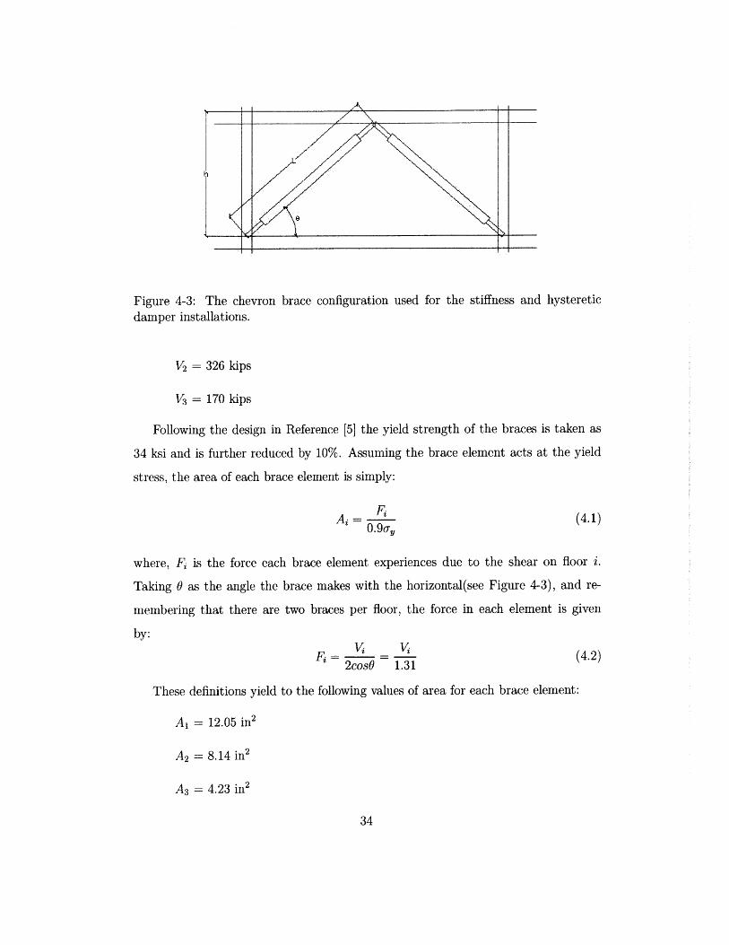
I _ 0

Figure 4-3: The chevrondamper installations.

brace configuration used for the stiffness and hysteretic

V2 = 326 kips

V3 = 170 kips

Following the design in Reference [5] the yield strength of the braces is taken as

34 ksi and is further reduced by 10%. Assuming the brace element acts at the yield

stress, the area of each brace element is simply:

(4.1)Ai = ^0.9ory

where, F is the force each brace element experiences due to the shear on floor i.

Taking 6 as the angle the brace makes with the horizontal(see Figure 4-3), and re-

membering that there are two braces per floor, the force in each element is given

by:

F - i * - (4.2)2cosO 1.31

These definitions yield to the following values of area for each brace element:

A1 = 12.05 in 2

A 2 = 8.14 in 2

A 3 = 4.23 in 2

34

In order to see the response of the structure under certain seismic loads, the stiffness

per floor was calculated using Equation 4.3.

A 2ki = 2 (A )Cos2o, (4.3)L i

The resulting stiffness values were then entered into MotionLab' No damping was

assigned to the structure in this analysis as the design procedure followed in this

section does not incorporate any damping. The low damping (i.e. 1-2%) provided

by the structural frame is ignored.

k, = 1258 kip/in2 = 220 MN/M 2

k2 = 850 kip/in2 = 149 MN/M 2

k3 = 442 kip/in2 = 77.4 MN/M 2

The displacement results from MotionLab indicated that the structure had deformed

more than the allowable limit defined in Section 4.1. The maximum displacement

observed on the third floor was u3 = 0.43 m, while the interstory displacement was

Au = 0.15 m.

4.3 Design with Hysteretic Dampers: Method 1

As the first step, the building is modeled as a discrete shear beam with lumped masses

(as calculated in Section 4.1) at story heights and varying lateral stiffness for each

floor. The stiffness per floor was calculated using the following equations:

For interior columns:12EIc

kint = 2~ (4.4)h3(1 + r)

For exterior columns:12EIc

kext = (4.5)h3(1 + 2r)

1MotionLab is a computer analysis software developed by J. J Connor. It analyzes lumped massmodels (in the linear region) using conventional or modal state-space formulations. It allows theanalyst to enter different values of mass, stiffness and damping values for each story.

35

where,

h: floor height

h Ib

E: Modulus of Elasticity

I, Moment of Inertia of the column

Ib: Moment of Inertia of the beam

Lb: Length of the beam

The calculations in Appendix B result in the following stiffness values:

k= 465 kip/in (81,440 kN/m)

k2= 411 kip/in (72,030 kN/m)

k3 = 188 kip/in (32,920 kN/m)

It should be mentioned that the bending deformation effects were neglected in these

calculations since experience shows that low-rise buildings such as the one under

investigation show a shear-beam response as opposed to a bending-beam response [6].

The modal shape observed when the original structure was subjected to BSE-1

excitation is given in Figure 4-4. Note that the modal shape gives relative values

of displacement, not absolute, as the displacement of each node is normalized with

respect to the maximum nodal displacement. Although the modal shape is close

enough to the desired modal shape (i.e. constant interstory displacement) for the

first mode the magnitude of the displacements, given below, are much higher than the

design limits specified Section 2.2. These two findings were the basis for attempting to

the bring the response of the building down to acceptable limits by applying damping

to the system, without increasing the stiffness.

U3 = 0.75m (29.53in) Au = 0.25m (9.84in)

T1 = 1.23sec T2 = 0.52sec T3 = 0.30sec

36

Modal displacement profile - real part - structure3

-0.6 -0.4 -0.2 0amplituc

0.2 0.4 0.6 0.8 1

Figure 4-4: The modal shape of the original structure subjected to BSE-1.

Many simulations were run with various values of ca, (the damping coefficient

per floor) with the objective of reducing the response. Results of some of the runs

are tabulated in Table 4.2. These results indicate that additional damping causes

considerable increase in the damping of the second and third modes, while, the modal

damping for the first mode is not as sensitive to the changes in the ca, value.

Around c,=5 500 000 Ns/m an interesting phenomenon was observed. The modal

periods and modal displacement profiles changed orders. As the value of the damping

coefficient was increased even further the second mode became overdamped and the

period of the second mode jumped up to around 600 seconds, which suggested that

the solution blew up and should be discarded. This unexpected phenomena is worth

investigating in greater detail. However, as it did not fit into the scope of this thesis,

the problem was avoided by selecting c, values that were smaller than the limiting

value.

37

- First mode- Second mode- - Third mode

-0-0.8

Table 4.2: Results of runs 1-6.

Run# ca,(MN-s/m) .j1(%) 2(%) 3(%) Ti(s) T2 (s) T3 (s) u3(m) Au(m)

1 1.50 7.0 21.5 23.0 1.23 0.53 0.31 0.260 0.0872 2.50 11.5 36.0 38.5 1.23 0.55 0.32 0.200 0.0673 3.50 15.5 51.0 54.0 1.23 0.57 0.33 0.175 0.0584 4.50 20.0 67.0 71.5 1.23 0.65 0.47 0.157 0.0525 5.00 22.0 74.0 81.0 1.23 0.69 0.58 0.157 0.0526 5.45 23.0 94.0 77.0 1.23 1.12 0.67 0.144 0.048

Change in Strategy

The initial strategy was to increase damping while keeping the stiffness constant

until the response of the structure was decreased to the allowable values. The value

of damping at which the structure's response was within the allowable values was

going to be taken as the upper limit for damping.

However, the phenomenon observed around ca, = 5 500 000 Ns/m lead to a

modification of the strategy. Damping coefficient of 5 450 000 Ns/m was taken as the

upper limit for damping and the stiffness values of each floor were adjusted. It should

be noted however, that the value of 5 450 000 Ns/m was the limiting value for the

damping coefficient, for the structure with no additional stiffness. As more stiffness

was added to the structure, the value of 5 450 000 Ns/m for damping was no longer

a limiting value and the overdamping of the second mode was avoided. The modified

strategy is as follows:

1. For the first run, enter the original stiffness values (i.e. the stiffness of the

original building, ki's used in Runs 1-6) as the initial stiffness values, however

utilize the "iterate on stiffness" option of MotionLab 2. As for the damping

coefficient value, use the upper limit value of c, = 5 450 000 Ns/m.

2. Record the displacement results.

3. For the subsequent runs, enter the original stiffness values as the initial stiffness

2The algorithm MotionLab follows consists of iterating on the stiffness values on a per floor basisuntil the displacements obtained are less than the design value. The outline of the algorithm can befound in Chapter 2 of [6].

38

values and click on the "iterate on stiffness" option, just like in Step 1. However,

pick different ca, values depending on the results from the previous run.

4. Record the displacement values and repeat Step 3 as many times as necessary,

until the displacements converge on the design values.

The results of the runs following this procedure are listed in Table 4.3.

The results of Run 7 show that the structure's response is under the maximum

allowable deformation. However, the values are considerably lower than the design

values, suggesting the existence of a more efficient design (i.e. a stiffness and damping

combination) that yields a response that is closer to the desired response. Just like

in any design, an iterative process is followed after Run 7 by changing the damping

values to obtain a response that is as close to the design response as possible.

Table 4.3: Results of Runs 7-10.

Run k1 k2 k3 Cay 1 2 63 U3 AU(MN/m) (MN/m) (MN/m) (MN-s/m) (%) (%) (%) (m) (m)

7 920 690 410 5.45 7.0 22.5 26.5 0.049 0.0168 720 520 280 9.50 15.0 48.0 53.0 0.053 0.0189 660 480 250 11.5 19.0 62.0 68.0 0.058 0.01910 650 480 240 12.5 21.0 68.5 26.0 0.058 0.019

Since the structure was "too stiff" in Run 7 a higher damping coefficient value

(ca=9 500 000 N-s/m) is used in the next run, leading to smaller iterated stiffness

values. The resulting displacement values are once again considerably lower than the

design values, hence value of the damping coefficient is increased once more to Ca,=

11 500 000 N-s/m in Run 9.

The results of Run 9 are "pretty good" and most likely adequate for preliminary

designs. However, an additional run was completed as a way to check that the results

really are converging on the design values. Although the displacement values obtained

from Run 10 were indeed closer to the design values, the difference was negligible.

It needs to be mentioned here that the controlling value for the iterations performed

on the stiffness values is the interstory displacement. The iterations continue until

39

the average of the interstory displacements is equal to the design value, which in this

case is 0.02m. If this happens to be an unsatisfactory or an inappropriate controlling

criteria, then one can use the stiffness values from the previous run, modify them

slightly and run a new analysis without iterations.

The results of Run 10 also indicate that increasing the damping coefficient to 12

500 000 N-s/m (8.6% increase) caused only a negligible decrease (1.4%) in the total

required stiffness of the building. This may be an important factor to consider for

design since the magnitude of total stiffness and damping are related to the cost. This

issue will be discussed in more detail in Chapter 6.

An additional factor that may be of importance is the number of iterations per-

formed on the stiffness values for each run. Table 4.4 shows how many iterations were

required to achieve the desired interstory displacement for each run. As one might

imagine, the more the iterations, the higher the cost of calculations, especially for

larger projects.

Table 4.4: Number of iterations required for Runs 7-10.

Run # of Iterations7 38 49 610 8

4.3.1 Conclusion

The results of this analysis shows that the original structure is extremely vulnerable

to BSE-1 earthquake and that its stiffness is about a magnitude smaller than what it

should be for the deformations to be acceptable. This confirms that moment frame

systems do not provide much lateral stiffness, even when hefty members are used. In

addition to being a moment frame, the relatively long bay widths, also caused the

effective lateral stiffness to be small for this particular building.

Most of the work involved in this method was about finding approximate values

40

for the optimal damping and stiffness values. Additional and sometimes considerable

number of iterations were necessary afterwards for fine-tuning the response.

4.4 Design with Hysteretic Dampers: Motion Based

Design Approach

The design approach followed in Section 4.3 consisted of increasing the stiffness of the

original building and adding damping to it until the desired response was achieved.

One can however, take a different approach to obtain close estimates to the stiffness

and damping values directly. This method, which is explained below, is taken from

[6] and is named the Motion Based Design (MBD) approach. Similar to the previous

method, once the approximate values of optimal stiffness and damping are obtained,

fine-tuning is necessary.

The starting point is the equilibrium equation for a damped system:

Mb*4+ C(D*q + KCD*q = P (4.6)

where, q is the displacement variable and the mass, M and the stiffness, K, matrices

are given as:

M1 0 0 k1 +k2 -k2 0

M= 0 m2 0], K= -k 2 k2 -+k3 -kj (4.7)

0 0 M3 0 -k3 k3

where the subscripts denote the story number.

The * matrix is the desired modal shape. Since the desired modal shape for

mode 1 corresponds to a constant interstory displacement, * is given as:

1/3

* = 2/3 (4.8)

1

41

The construction of the damping matrix, C depends on how the designer wishes to

vary the damping throughout the structure. In this study, damping is distributed

uniformly between the three floors, i.e. every floor has the same damping coefficient,

Cay. For this type of damping distribution the C matrix has the same form as the K

matrix:

C1 + C2 -C2 0 2Cav -Cav 0

C [-C2 C2 + C -C3 = cav 2Cav -Cav (4.9)

0 -C3 C3 0 -Cav Cav

Since in seismic excitations the nodal forces are proportional to the nodal masses, the

force matrix, P is defined as:

MI

P = -ag m2 (4.10)

M3)

where mi are the floor masses and ag is the ground acceleration.

Multiplying Equation 4.6 by (<D*)T yields:

in-4 + q + Iq = P (4.11)

where the quantities with superscript tilde are equivalent one degree of freedom mass,

damping, stiffness and force quantities. They are defined and calculated as:

i = ()*)TM(* = 7.836 x 105kg (4.12)

a = (,*)TCb* = 2 w(hn (4.13)

kW 2fn (4.14)

S=(lt*)Tp (4.15)

j is usually expressed in terms of the equivalent mass, ?'n- and the modal participation

factor, F, as:

= -Fhag (4.16)

42

where,

r = . * - 1.271M

(4.17)

Using these definitions and results, the stiffness for each floor is obtained. During the

process one utilizes the response spectra shown in Figure 4-5. Since the maximum

100

EI

101

5

10 -

10,

101

-- - - ........I ...

-. - -... .... ........ ............: .....

............... ~~~~- ... .. p..ng. ....... .. . . . . . . . . . ... 2................................................ Damping.. .. t. ....... ..

.. ~~~~~~~~~ ~ ~ ~ ~ ~ .a p n .a i . .. -.

.~~~~~~ ~ ~ ~ ~ .a p n .a i . . .......1 . ... .. . . ..............~~~~- ... .. .p.. .ng. R.. ... .. .. .. .. 2. .

10100Period - seconds

Figure 4-5: Response Spectra for BSE-1.

allowable maximum displacement is u* = 0.06m at the top, from the response spectra,

one can obtain what the period of the structure should be by assuming a damping

ratio for the system. However, since response spectra plots are for SDOF systems,

one uses the modal participation factor F to express the current 3-DOF problem as

a SDOF problem. Hence, the design spectral displacement is:

S = -U3 = 0.0467m (4.18)

In this study the stiffness calibration was based on a damping ratio of, = 20%. This

damping ratio along with the maximum allowable shear deformation lead to a struc-

43

ture with a period of T = 0.50 seconds (from Figure 4-5). The stiffness distribution

that yields that period value is:

472

k = 396 x 10 6N/m (4.19)

245)

The damping coefficient per floor is obtained by:

c = 2w&n = -cay (4.20)3

cay = 11.8 x 10 6N-s/m (4.21)

These values of stiffness and damping should theoretically yield a response that is

equal to the design limit. As a check these values are entered into MotionLab, the

response is observed and modifications are made in a fashion similar to the method

of Section 4.3. Results of these runs, Runs 101-106 are listed in Table 4.5.

Table 4.5: Results of Runs 101-106.

Run k, k2 k3 Cay ' 2 3 U3 AU

(MN/m) (MN/m) (MN/m) (MN-s/m) (%) (%) (%) (m) (m)101 472 397 245 11.8 20.0 62.0 81.0 0.078 0.026102 472 397 245 13.0 22.0 90.0 68.0 0.075 0.025103 700 510 360 13.0 22.0 67.0 77.0 0.052 0.017104 650 500 330 13.0 19.0 58.5 77.0 0.052 0.017105 550 450 330 13.0 20.0 59.0 82.0 0.062 0.021106 570 440 330 13.0 20.0 83.0 58.0 0.060 0.020

During Runs 101-103 the limiting value for the damping coefficient was found to

be cav=13 000 000 N-s/m. On Run 103, the iteration function was selected, so that

the stiffness values would be iterated until an interstory displacement of Au = 0.020m

is obtained. However, results of Run 103 and some intermediate runs that are not

given here, showed that the iterations caused the building to be too stiff. Therefore in

Runs 104 to 106 manual iterations were performed based on the result of the previous

run, until the desired response was achieved.

44

4.4.1 Conclusion

In the MBD approach stiffness and damping values that yield approximately the

design deformations are obtained initially following a simple algorithm introduced

above. Then, several manual "iterations" are necessary to achieve the design criteria.

The main difference between MBD approach and approach of Method 1 is the amount

of flexibility (and hence responsibility) given to the designer. The designer needs to

be able to interpret the results of a run properly in order to make the necessary

modifications on certain parameters for the next run. In addition, the number of

iterations required in Run 103 was only one. Attaining an approximate value for

stiffness using the MBD approach required less iterations. Again this may have

significant impact on the cost of the calculations for larger scale projects.

45

46

Chapter 5

SAP Analyses

5.1 Introduction

In Chapter 4, three design methodologies were presented, one being the more tra-

ditional Strength Based Design. The latter two methodologies are associated with

damage controlled design and introduce stiffness and damping to the structural sys-

tem. In this chapter the optimal design values obtained in Chapter 4 will be input

into SAP2000 1 to observe the structure's response under BSE-1 and BSE-2 loadings.

Since the Performance Level to be used for design purposes allows the structure to

enter the nonlinear region under BSE-2 loading, the use of SAP2000 Nonlinear was

necessary.

It was previously shown, in Section 4.2 that the structure resulting from the

Strength Based Design would experience unacceptable deformations even under BSE-

1 loading. Therefore, that design approach is discarded. Although the remaining two

methods were very similar in nature the results of the Motion Based Design Approach

will be used here simply because it is the approach that provided the designer with

more flexibility and responsibility during the process.

1A widely used finite element structural analysis program produced by Computers & Structures,Inc.

47

5.2 Input

The first step in the SAP2000 analysis was to enter the geometry of the building

and then to assign sections to the frame members in accordance with the original

building. After this was completed the two loading Time History Functions and

Cases were defined for the BSE-1 and BSE-2 excitations.

Then the retrofit began, i.e. the additional stiffness and dampers were installed

using the chevron brace configuration. Both the braces that provide the stiffness

and the damping elements were defined as NonLinearLink (NLLink) elements, as

discussed in the next section. For analysis purposes that the dampers and the main

lateral stiffness members were placed in different bays for reasons of clarity2 . During

actual construction the location of these elements would be governed by other factors,

such as accidental torsion effects. It should be noted however, there is no reason for

the dampers not to be put in the same bay as the braces that provide stiffness. How

the necessary properties for the stiffness and damper members were obtained and

entered into SAP2000 are explained next.

5.2.1 Assigning the "optimal" stiffness and damping values

From the results of the Motion Based Design approach required stiffness and damping

values per floor are given as:

k1 = 570 MN/m = 3255 kip/in

k2 = 440 MN m = 2512 kip/in

k3 = 330 MN/m = 1884 kip/in

The first thought that comes to mind is to provide the total floor stiffness by the

brace elements, which are the traditional braces using normal 36ksi steel, and add the

dampers totally separately. The dampers themselves would be providing some lateral

2 The analyses were performed using only a two bay structure, rather than the four bay structure.

This simplification could be made, since eliminating the additional stiffness provided by the bending

of the members in the other bays lead to a more conservative analysis.

48

stiffness, however that value could be kept to a negligible magnitude by adjusting the

length of the yielding core element since the stiffness is given by:

SAEL

where L is the length of the yielding element.

However, the analysis of the structure revealed that the damping mechanism was

not functioning at all. The time history plot in Figure 5-1 clearly shows there is

practically no force taken by the damper elements. This was confirmed when the

response was checked and found to be close to that obtained in the case with no

damping. Although, surprising and discouraging at first, these results were justified

and rationalized shortly after. Load will always follow the path of most stiffness to

find its way to the foundations. Since all of the stiffness in the structure is provided by

the brace elements, all of the lateral load is resisted by them as well, leaving negligible

forces to be experienced by the dampers. The magnitude of the forces the dampers

experienced were not large enough to cause the necessary yielding for damping to

take effect.

a.

Ua-0IL

4

2

0

-2

-6

40 50 6020 30

Time (sec)0 10

Figure 5-1: The force experienced by the dampers is negligible,dampers have a yield strength of 386.4 kips

considering the

49

ALLAI "AIL --1 04

This realization lead to a solution in which the required lateral stiffness per floor

was divided between the dampers (kd) and the braces (kb). How one would design

the elements to achieve these values in real life is discussed in the following sections.

A more complicated issue is determining the optimal distribution of the total story

stiffness (k,) between the dampers and the braces. The distribution should be done

such that the dampers "draw" enough force to yield as many times as possible during

the excitation. However, the distribution should also be such that,

kd

kb ~

This criteria ensures that the stiffness provided by the dampers is at most equal to

that provided by the braces. Ideally this ratio should be as small as possible, because

hysteretic damper elements are designed to be replaced every so often3 and it is not

desirable for the structure to lose a significant amount of its lateral resistance during

the replacement process. Depending on the owner's and/or the designer's wishes, this

criteria could be made more stringent.

The theoretical method to arrive at the correct distribution of the story stiffness,

k., and why that methodology was deemed inappropriate is discussed in the following

sections. As an alternative to the theoretical approach, numerical simulations were

run using SAP2000 with varying parameters to attain relationships that can be used

to determine the ideal stiffness distribution.

As mentioned in Section 5.2, both the stiffness braces and the dampers are modeled

as NLLink members in SAP2000, because it is expected that especially under BSE-2

both mechanisms may go into the plastic region. The Plastic type NLLink elements

in SAP2000 are those that have an initial stiffness until yielding and a reduced,

secondary stiffness post-yielding. As such, this type of NLLink elements are deemed

to be most appropriate to model both the braces and the dampers. Figure 3-3 shows

3These elements can only take up to a certain number of cycles, after which they become inef-

fective. The number of cycles until that stage is reached varies with many factors and is a design

parameter that needs to be considered. For the purposes of this study, it is adequate to say that the

hysteretic dampers are designed to be replaced

50

the idealized Force-deformation curve for a elastic-perfectly plastic4 material.

Figure 5-2 shows the dialog box one uses to enter the properties of a plastic

NLLink element. There are two sections to fill in this dialog box; Linear Properties

and NonLinear Properties. The Effective Stiffness and the Stiffness values in these

sections refer to the same parameter, and should be assigned the value of the stiffness

of the member in the elastic region. Effective damping box is not applicable to

neither the hysteretic dampers nor the stiffening braces, hence value of zero should

be assigned. The yield strength is the magnitude of the force required to yield the

element. The Post Yield Stiffness Ratio is the ratio of the post yield stiffness to

stiffness (or effective stiffness). Since both elements are idealized as elastic-perfectly

plastic this ratio is taken as zero as well5 . The yielding exponent is kept at its default

value of 2.

The two parameters one can utilize to attain the optimal stiffness distribution are

the stiffness and the yield strength for both the dampers and the braces. To see how

the response of the structure was related to these two parameters a total of 12 runs

were performed. In these runs the stiffness distributions were:

Runs 1-4: kd = 50% k, and kb = 50% k,

Runs 5-8: kd = 30% k, and kb = 70% ks

Runs 9-12: kd = 10% k, and kb = 90% k,

The stiffness distribution schemes are named as 50-50, 30-70 and 10-90, where the

first number specifies the percentage of story stiffness provided by the dampers and

the second number specifies the percentage of stiffness provided by the braces. For

instance in Runs 5-8, 70% of the total desired story stiffness, (see beginning of Sec-

tion 5.2.1) is to be provided by the brace elements. Hence their cross-sectional areas

4 Perfectly plastic means post-yield stiffness is zero'A very small value such as 0.0001 is used for analysis purposes, because entering zero creates

instabilities in the structure

51

are designed to give the following stiffness values per floor.

k = 70%(3255) kip/in = 2279 kip/in (5.1)

k = 70%(2512) kip/in = 1758 kip/in

k = 70%(1884) kip/in = 1319 kip/in

Each stiffness distribution lead to new values of yield strength for the braces,

which was calculated by the following formulas:

.LA'=2k (5.2)

b s2ECOs20

FZ =Aloi (5.3)

where superscript i denotes the story number, subscript y stands for "yield", L is

the length of the brace element, and 0 is the angle the brace element makes with the

horizontal.

For each stiffness distribution 4 values of damper yield strengths were considered

to vary the effective damping and observe the effect on the response of the structure.

These values correspond to a maximum value of Fd,= 368.4 kips and fractions of that

maximum value. Selection of Fd,= 368.4 kips is justified in Section 5.4. Note that

the same yield strength is used for all floors, since this parameter is kept constant

throughout the building in this analysis.

5.3 Results and Interpretation

Table 5.1 provides the maximum displacement observed at the top floor for BSE-1

and BSE-2 excitations for these 12 runs.

Figures 5-3 - 5-5 show how the response of the structure varies with the yield

strength of the dampers and how it relates to the design displacements for BSE-1 and

BSE-2 (shown as thick horizontal lines). Here are some of the conclusions that can

52

Table 5.1: Results of Runs 1-12.

Run Stiffness Fda U3max (in) drift (%)Distribution (kip) BSE-1 BSE-2 BSE-1 BSE-2

1 50 - 50 368.4 6.532 10.61 1.40 2.272 184.2 7.302 11.37 1.56 2.433 122.8 7.385 11.56 1.58 2.474 92.10 7.720 11.83 1.65 2.535 30 - 70 368.4 4.273 8.045 0.91 1.726 184.2 5.217 9.130 1.11 1.957 122.8 5.740 9.875 1.23 2.118 92.10 6.050 10.18 1.29 2.189 10 - 90 368.4 5.473 6.537 1.17 1.4010 184.2 4.283 7.134 1.12 1.4611 122.8 5.224 6.847 0.92 1.5212 92.10 5.036 7.356 1.08 1.57

be drawn from these graphs:

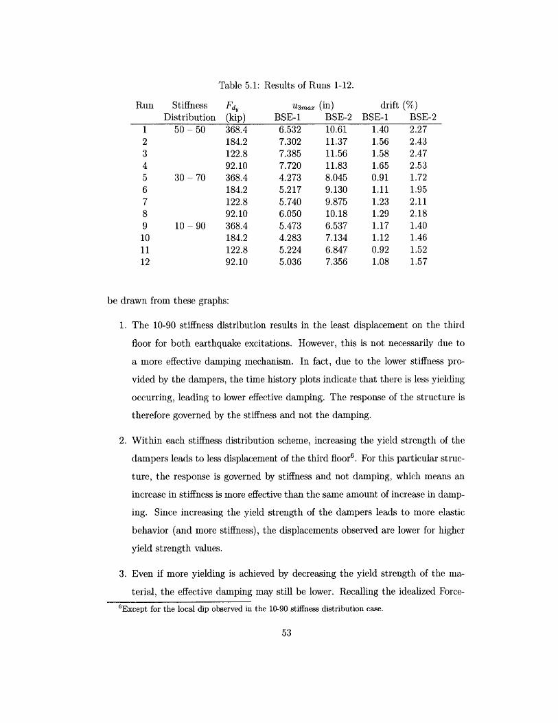
1. The 10-90 stiffness distribution results in the least displacement on the third

floor for both earthquake excitations. However, this is not necessarily due to

a more effective damping mechanism. In fact, due to the lower stiffness pro-

vided by the dampers, the time history plots indicate that there is less yielding

occurring, leading to lower effective damping. The response of the structure is

therefore governed by the stiffness and not the damping.

2. Within each stiffness distribution scheme, increasing the yield strength of the

dampers leads to less displacement of the third floor 6 . For this particular struc-

ture, the response is governed by stiffness and not damping, which means an

increase in stiffness is more effective than the same amount of increase in damp-

ing. Since increasing the yield strength of the dampers leads to more elastic

behavior (and more stiffness), the displacements observed are lower for higher

yield strength values.

3. Even if more yielding is achieved by decreasing the yield strength of the ma-

terial, the effective damping may still be lower. Recalling the idealized Force-6Except for the local dip observed in the 10-90 stiffness distribution case.

53

deformation plot in Figure 3-3, it can be seen that less energy dissipation (i.e.

less area inside the curve) is achieved with decreasing yield strength. Hence the

optimal yield strength is a function of the interaction of these two phenomena:

Amount of yielding and size of the Hysteresis loop.

4. None of the stiffness distribution and yield strength combinations resulted in a

structure that satisfied the displacement criteria for BSE-1. This is surprising

since, previous analyses in Chapter 4 had shown that certain combinations

of stiffness and damping per floor would result in a satisfactory design. The

reason, for the discrepancy between two analyses has to do with how hysteretic

damping is modeled as an equivalent viscous damping and is discussed further

in Section 5.4.

5. It is possible to achieve a response that satisfies the design criteria for BSE-

2 excitation. This is partially due to an increase in the effectiveness of the

hysteretic dampers for larger excitations.

Concluding that the structure's response is dominated by stiffness has significant

consequences. It suggests that damping does not contribute significantly to the design,

and the best design consists of stiffness only (i.e. no damping). Section 5.4 attempts

to explain the reasons for this and other unexpected results of these runs.

5.4 What Went Wrong?

As mentioned earlier, analyses performed by MotionLab and discussed in Chapter 4

suggested that damping had a significant effect on the response of the building. How-

ever, in the previous section it is concluded that stiffness is the only important factor.

What is the reason for this paradox?

54

5.4.1 Expressing Hysteretic Damping as Equivalent Viscous

Damping

In fact there is no paradox. The conclusion drawn in the previous section is only true

for hysteretic dampers. The root of the problem lies in the expression used to convert

hysteretic dampers into equivalent viscous dampers. The conversion formula, Equa-

tion 5.47, holds true if the excitation is periodic with an amplitude ii and frequency

Q and if in every cycle the material yields.

Fjz = ( Ca (5.4)- 4 -1

where p is the ductility ratio, defined as the ratio of the maximum extension of the

member to the extension at which the member yields.

Figures ?? and ?? show the Time Histories of the forces the hysteretic damping

elements in the first story experience. The dampers were given a yield strength of

122.8 kip in this particular case. A careful examination of the plot shows that the

dampers reach the yielding point many more times for the BSE-2 excitation, hence

making the effective damping larger for that case. In fact, if the excitation was so large

that the elements yielded at every cycle, Equation 5.4 would work almost8 perfectly.

In other words, Equation 5.4 represents the ideal case in which the energy dis-

sipation is maximized. When the correct value are given to the parameters in that

equation, the yield strength one obtains is 368.4 kips. That is why that value was

taken as the maximum value for the yield strength of the hysteretic dampers. A value

more than that would result in no yielding for some of the cycles in the loading, which

corresponds to linear behavior and no energy dissipation hence less effective damping

(i.e. no area within the Force-displacement curve).

This also justifies the attempts to increase the effective damping by decreasing

the yield strength of the dampers. When one looks at Equation 5.4, it is clear that

7 This formula is based on equating the energy dissipated per cycle of excitation to that of a linearviscous damper.

8 "Almost" because the frequency of the excitation is not constant and the natural frequency ofthe structure is used to replace ( in Equation 5.4

55

taking a smaller value for R would mean a smaller value for Fde and therefore allow

the elements to yield earlier and more frequently, ideally every cycle, during the

excitation. However, as mentioned earlier, whether decreasing the yield strength of

the member achieves more effective damping depends on an additional factor. Since

energy dissipation per cycle is given by the area within the Force-deformation curve

(see Figure 3-3), there is a limit as to how low the yield strength should be.

5.4.2 The Earthquake

The design earthquake chosen for this study was the Imperial Valley 1940 earthquake,

because it is a representative earthquake for the Mid-California region; the region that

is of most interest in the United States. As the time history of the ground acceleration

in Figure 2-3 shows, this earthquake shows an impulsive behavior, meaning that it

reaches its peak ground acceleration (PGA) of 134.5 in/sec2 (3.42 m/sec2 ) very early

on and doesn't get close to that maximum value many times after that. It is not hard

to see that this type of earthquake is probably the farthest one away from a periodic

loading, for which Equation 5.4 holds. A study with a larger variety of earthquakes

would yield more acceptable and reliable results.

56

Figure 5-2: The dialog box in SAP2000 where the properties of NLLink elements aredefined.

57

50-50 St01ness DisfIbution

w VA zo 260 3w, 390 twYW4i Wtrnoth (ktp)

Figure 5-3: Maximum displacement observed on third floor vs.dampers for 50-50 stiffness distribution scheme.

30-70 SWfmsm DIutrlbution

I

4-080

900-

Y141d *Is011Uth01P)

Figure 5-4: Maximum displacement observed on third floor

dampers for 30-70 stiffness distribution scheme.1040 SMnSS DilOIU n

V

A

vs.

7

- --- 650.1

2 - -2

so 10D 19D 3wSOS 4w

Figure 5-5: Maximum displacement observed on third floor vs.

dampers for 10-90 stiffness distribution scheme.

58

yield strength of

9

yield strength of

yield strength of

9

BSE-1 ExcItatIon

I.10

S 10 Is 2 25 30 35 40 45 so 56

Time(9

Figure 5-6: Time history of the force the hysteretic dampers (F, 122.8 kips) inthe first story experience under BSE-1 excitation.

200

Figure 5-7: Time history of the force the hysteretic dampers (F, = 122.8 kips) inthe first story experience under BSE-2 excitation.

59

60

Chapter 6

Cost Study

An important consideration in every engineering solution is the cost associated with it.

As mentioned earlier, the optimal solution to a civil engineering problem is one that

provides satisfactory results within the cost limits determined prior to the project.

Since this thesis proposes several concepts and methodologies one could follow to

attain the desired performance, it is fitting to discuss the cost associated with each

of the solutions.

Due to the limited amount information available on costs associated with the

design, manufacturing and installation of hysteretic dampers, a very detailed cost

analysis will not be presented here. What is of greater interest is the factors affect-

ing the cost of the whole project and their relative importance in the overall cost

calculations. In that respect only the costs associated with the hysteretic dampers

and the primary lateral support system will be of interest. In addition, no such

costs as construction costs will be considered, but rather the material costs will be

investigated.

6.1 Cost of the Primary Lateral Support System

The primary lateral support system in this retrofit example consists of pairs of chevron

braces, made out of steel. In the construction industry, for ordinary steel, the pricing

is done on a per weight units. Hence, determining the weight of the steel used should

61

be adequate for understanding how the cost varies with stiffness. The process to find

the relationship between the stiffness and the cost of the material is presented below:

C=pW

W = y AL

A= LA = k2ECOs20

p: Price of steel per weight

C: Cost

W: Weight of Steel used

m: Weight density of steel

A: Cross-sectional area

L: Length of steel

k: Stiffness of each element

E: Modulus of elasticity for steel

C = p E 2 0 k2Ecosg

.-. C = f >k f: A factor

The final line states that the cost of steel is directly proportional to the sum of

the stiffness values provided by these steel members throughout the structure.

6.2 Cost of the Hysteretic Dampers

Establishing a relationship between the cost of hysteretic dampers and the effective

damping due to those dampers is more involved than it is for stiffness members.

Assuming that Equation 5.4 holds, one can rewrite it as:

Cay - ( 4 1)c7,=F(6.1)

62

Assuming the length of the damper is fixed, the amount of damping achieved is a

function of the yield strength, which can be correlated to the required area through

the yield stress, a material specific parameter. Therefore it can be concluded that

damping and cross-sectional area of the hysteretic damper are inversely proportional:

1Cay =q-

where g is a factor. Assuming the cost is related only to the volume of the yielding

material used and the total length of hysteretic dampers is fixed, the cost is inversely

proportional to the damping desired on each floor. In other words, the owner would

pay less to achieve more damping.

1Cost = h

Cay

In reality however this conclusion will not hold, simply because the cost is not deter-

mined only by the amount of material to be used. There are many other factors that

need to be incorporated into the cost analysis, such as:

1. Costs associated with using proprietary material.

2. Initial costs incurred in producing and marketing the material.

3. Economies of scale that may prevail if large production facilities exist.

4. The competitiveness in the market for energy dissipation devices.

As hysteretic dampers and energy dissipation devices in general, are relatively new

concepts, there are many ambiguities associated with their costs. Enough time needs

to pass for hysteretic dampers to become more of a commodity, rather than a propri-

etary idea, for cost calculations to be as simple and direct as those for steel members.

63

6.3 Cost of the Retrofit

The different design methodologies presented in Chapter 4 resulted in different com-

binations of damping and stiffness values that produce an acceptable design. In fact,

number of possible stiffness-damping combinations could be increased even further

by performing more numerical simulations. Therefore there is no single number for

the cost of a retrofit project. To obtain the optimal stiffness-damping combination in

terms of cost, one would generate a number of more stiffness-damping combinations

that work and then evaluate the cost of each one to determine the lowest cost one.

An additional complexity in the cost calculations exists due to the fact that the

hysteretic dampers need to generate stiffness as well as damping for the damping

mechanism to function effectively. Since the stiffness provided by the damper is

related to its geometric properties such as area and length, there exist many possible

designs even for one stiffness-damping combination.

64

Chapter 7

Conclusion

Studies show that the traditional Strength Based Design methodology is becoming

inadequate in responding to the changes in the construction industry, such as the

increase in costs of repairs and insurance. As owners become more aware of this fact

and attain a better understanding of structural performance levels, there will be a

trend towards the use of Damage-Controlled Structures. These structures involve the

use of energy dissipation devices to restrict the deformation and therefore the damage

of the structure.

The Motion Based Design Approach is recommended here for establishing the

stiffness and damping combinations required for the structure's response to be within

the design limits. Then cost analysis should be performed to identify the optimal

stiffness and damping combination.

The use of hysteretic dampers in Damage-Controlled Structures is common in

Japan and is expected to increase in the United States. These devices can be used to

attain the optimal stiffness and damping combination that are determined in earlier

steps of the design process. However, simulations show that it is difficult to achieve the

desired effective damping by using hysteretic dampers due to the assumptions made

when expressing hysteretic damping as equivalent viscous damping; a necessary step

for the design. In specific, inaccuracies arise due to the fact that the earthquake loads

are not periodic functions with constant frequencies.

The effective damping generated by hysteretic dampers is represented by the area

65

bounded by the Force-displacement curve for the member. Therefore increasing the

yield strength of the damper should lead to an increase in the energy dissipation.

However, there is a limit to how high the yield strength should be because the hys-

teretic damper should yield considerably earlier than the primary structure. Finding

the optimal yield strength for the hysteretic damper is the main challenge in design

process.

The simulations show that the desired response of the three-story structure ana-

lyzed in this thesis cannot be achieved by using hysteretic dampers. However, one of

the reasons is the impulsive characteristics of the representative earthquake used in

the analyses. A wide range of earthquakes should be incorporated into the analysis

in order to obtain more reliable conclusions.

66

Appendix A

Los Angeles Ground Motion

Records

Table A. 1: 50/50 Set of Records (72 years Return Period). Taken from [3]

Designation Record Info Duration

(sec)Magnitude(Mw)

R(km)

Scale

LA41 Coyote Lake, 1979 39.38 5.7 8.8 2.28LA42 Coyote Lake, 1979 39.38 5.7 8.8 2.28LA43 Imperial Valley, 1979 39.08 6.5 1.2 0.40LA44 Imperial Valley, 1979 39.08 6.5 1.2 0.40LA45 Kern, 1952 78.60 7.7 107.0 2.92LA46 Kern, 1952 78.60 7.7 107.0 2.92LA47 Landers, 1992 79.98 7.3 64.0 2.63LA48 Landers, 1992 79.98 7.3 64.0 2.63LA49 Morgan Hill, 1984 59.98 6.2 15.0 2.35LA50 Morgan Hill, 1984 59.98 6.2 15.0 2.35LA51 Parkfield, 1966, Cholame 5W 43.92 6.1 3.7 1.81LA52 Parkfield, 1966, Cholame 5W 43.92 6.1 3.7 1.81LA53 Parkfield, 1966, Cholame 8W 26.14 6.1 8.0 2.92LA54 Parkfield, 1966, Cholame 8W 26.14 6.1 8.0 2.92LA55 North Palm Springs, 1986 59.98 6.0 9.6 2.75LA56 North Palm Springs, 1986 59.98 6.0 9.6 2.75LA57 San Fernando, 1971 79.46 6.5 1.0 1.30LA58 San Fernando, 1971 79.46 6.5 1.0 1.30LA59 Whittier, 1987 39.98 6.0 17.0 3.62LA60 Whittier, 1987 39.98 6.0 17.0 3.62

67

PGA(in/sec

2)

227.7128.755.443.155.761.4130.4118.8123.0211.0301.4243.8267.7305.1199.8146.397.789.2296.7184.7

Table A.2: 10/50 Set of Records (475 years

Record Info

Imperial Valley, 1940Imperial Valley, 1940Imperial Valley, 1979Imperial Valley, 1979Imperial Valley, 1979Imperial Valley, 1979Landers, 1992Landers, 1992Landers, 1992Landers, 1992Loma Prieta, 1989Loma Prieta, 1989Northridge, 1994, NewhallNorthridge, 1994, NewhallNorthridge, 1994, RinaldiNorthridge, 1994, RinaldiNorthridge, 1994, SylmarNorthridge, 1994, SylmarNorth Palm Springs, 1986North Palm Springs, 1986

Duration

(sec)39.3839.3839.3839.3839.0839.0879.9879.9879.9879.9839.9839.9859.9859.9814.9514.9559.9859.9859.9859.98

Return Period). Taken from [3]

Magnitude(Mw)6.96.96.56.56.56.57.37.37.37.37.07.06.76.76.76.76.76.76.06.0

R(km)10.010.04.14.11.21.236.036.025.025.012.412.46.76.77.57.56.46.46.76.7

Scale PGA(in/sec2

)2.01 178.02.01 261.01.01 152.01.01 188.40.84 116.40.84 90.63.20 162.63.20 164.42.17 200.72.17 139.11.79 256.91.79 374.41.03 261.81.03 253.70.79 206.00.79 223.90.99 219.90.99 315.52.97 393.52.97 380.9

Table A.3: 2/50 Set of Records (2475 years Return Period). Taken from [3]

Designation Record Info Duration(sec)

1995 Kobe1995 Kobe1989 Loma Prieta1989 Loma Prieta1994 Northridge1994 Northridge1994 Northridge1994 Northridge1974 Tabas1974 TabasElysian Park (simulated)Elysian Park (simulated)Elysian Park (simulated)Elysian Park (simulated)Elysian Park (simulated)Elysian Park (simulated)Palos Verdes (simulated)Palos Verdes (simulated)Palos Verdes (simulated)Palos Verdes (simulated)

59.9859.9824.9924.9914.9514.9559.9859.9849.9849.9829.9929.9929.9929.9929.9929.9959.9859.9859.9859.98

Magnitude(Mw)6.96.97.07.06.76.76.76.77.47.47.17.17.17.17.17.17.17.17.17.1

H.R(km)3.43.43.53.57.57.56.46.41.21.217.517.510.710.711.211.21.51.51.51.5

Scale PGA(in/sec2 )

1.151.150.820.821.291.291.611.611.081.081.431.430.970.971.101.100.900.900.880.88

495.3355.4161.4182.6335.3364.3357.8513.4312.4382.9500.5458.1302.1262.8383.1424.9274.7299.7193.1241.4

68

Designation

LA01LA02LA03LA04LA05LA06LA07LA08LA09LA10LA11LA12LA13LA14LA15LA16LA17LA18LA19LA20

LA21LA22LA23LA24LA25LA26LA27LA28LA29LA30LA31LA32LA33LA34LA35LA36LA37LA38LA39LA40

Appendix

Stiffness

Original

Calculations for the

Structure

69

B

Stiffness Calculations for the example building given in FEMA 355C. LA version.

Ib 1:= 5900in

Ib2 := 4930in

lb3 := 183011

Lb:= 360in

h:= 156in

IcA:= 3400in4

IcB:= 4330in4

Ic= 4330in4

IcD: 34000

IcE:= 723in4

I CA]LbrIA:= - -_

h Lb1

ICA Lb

ICA Lbt3A:= -- 1

h Ib2

Icc it1U h Ib,

IC Lb IcC 4b:= --- r :=

hPIb hIb2

ICB Lbh Ib3

Icc Lb.h Ib3

E:= 29000000psi

ICD LbrID

h Lb1

ICD Lbh Ib2

ICD Lbh Ib3

12-E-IcA

h(1 + 2-rA)

12-E-IcA

h3(1 + 2-rA)

12-E-IcAk3A:=

h3(1 + 2-r3A)

ki kIA + kiB + kic + kiD

k2 k2A + k2B + k2C + k2D

k: k3A + k3B + k3C + k3D

12-E-Ic

h3(1 + r28)

12-E-IcB12B 2

h 3(1 + r2B)

12-E-IcBk3B:=

h3(1 + r3B)

kc=-12-E-IcC

h3(1 + rnc)

12-E-Icc

h3(1 + r2c)

12-E-Icc

h3(1 + r3c)

k1=8-144x10-m

7 Nk2 = 8.144 x 10 -

k2 =7.203 x Gm

k3 = 3.292x 167M

k = 4.65 x d03- in

k2 = 4.113 X d _

5 lbfk3 = 1.88 x 10 --

in

12-E-cD

h3(l + 2-rD)

12-E-IcDk2D

h 3(1 + 2-r2D

12-E-IcDk3D

h3(1 + 2-r3D)

70

ICB Lbh IbI

Bibliography

[1] FEMA-273: NEHRP Guidelines for the Seismic Rehabilitation of Buildings.

Technical report, Federal Emergency Management Agency, 1997.

[2] Automated Production of Low Cost Pultruded Composite Bracing for Seismic

Energy Dissipation Structures: Phase I Final Technical Report. Technical report,

Kazak Composites Incorporated, 2000.

[3] FEMA-355C: Systems Performance of Steel Moment Frames Subject to Earth-

quake Ground Shaking. Technical report, Federal Emergency Management

Agency, 2001.

[4] Parry Brown, Ian D. Aiken, and F. Jeff Jafarzadeh. Seismic retrofit of the

Wallace F. Bennett Federal Building. Modern Steel Construction, August 2001.

[5] Peter Clark, Ian Aiken, Eric Ko, Kazuhiko Kasai, and Isao Kimura. Design

procedures for buildings incorporating hysteretic damping devices.

[6] J. J. Connor. Introduction to Structural Motion Control in progress.

[7] J. J. Connor and A. Wada. Performance based design methodology for structures.

In Proc., Int. Workshop on Recent Developments in Base-Isolation Techniques

for Buildings, Tokyo, Japan, 1992. Arch. Institute of Japan.

[8] J. J. Connor, A. Wada, M. Iwata, and Y.H. Huang. Damage-Controlled Struc-

tures. I: Preliminary design methodology for seismically active regions. Journal

of Structural Engineering, 123(4):423-431, 1997.

71

[9] A. Wada, J. J. Connor, H. Kawai, M. Iwata, and A. Watanabe. Performance

based design methodology for structures. In Proc., 5th U.S.-Japan Workshop

on the Improvment of Build. Struct. Des. and Constr. Practices. Appl. Technol.

Council, 1992.

[10] Akira Wada, Yi-Hua Huang, and Mamoru Iwata. Passive damping technology

for buildings in Japan. Prog. Struct. Engng. Mater., (2):335-350, 2000.

72