1

IIIdddiiiooommmaaattteeerrriiiaaalll UUUnnniiivvveeerrrssseee:::

TTThhheee UUUNNNUUUMMM aaasss MMMooonnnoooiiidddaaalll CCCaaattteeegggooorrryyy ooofff

OOObbbjjjeeeccctttsss aaannnddd MMMooorrrppphhhiiisssmmmsss aaasss CCCooonnntttiiinnnuuuuuummm

MMMuuullltttiiillleeevvveeellleeeddd MMMaaannniiifffooolllddd ––– AAA WWWooorrrkkk iiinnn

PPPrrrooogggrrreeessssss ooofff NNNeeeeeedddeeeddd MMMaaattthhheeemmmaaatttiiicccsss aaannnddd

PPPrrrooobbbllleeemmmsss AAAhhheeeaaaddd

AAA... RRR... BBBOOORRRDDDOOONNN LLLiiifffeee PPPhhhyyysssiiicccsss GGGrrrooouuuppp --- CCCaaallliiifffooorrrnnniiiaaa

LLLiiimmmiiittteeeddd CCCiiirrrcccuuulllaaatttiiiooonnn,,, MMMaaayyy 222000000444 ––– EEEdddiiittteeeddd JJJuuunnneee---JJJuuulllyyy,,, 222000000999

2

IIIdddiiiooommmaaattteeerrriiiaaalll UUUnnniiivvveeerrrssseee:::

TTThhheee UUUNNNUUUMMM aaasss MMMooonnnoooiiidddaaalll CCCaaattteeegggooorrryyy ooofff OOObbbjjjeeeccctttsss aaannnddd

MMMooorrrppphhhiiisssmmmsss aaasss CCCooonnntttiiinnnuuuuuummm MMMuuullltttiiillleeevvveeellleeeddd

MMMaaannniiifffooolllddd ––– AAA WWWooorrrkkk iiinnn PPPrrrooogggrrreeessssss ooofff ttthhheee NNNeeeeeedddeeeddd

MMMaaattthhheeemmmaaatttiiicccsss aaannnddd PPPrrrooobbbllleeemmmsss AAAhhheeeaaaddd

AAA... RRR... BBBOOORRRDDDOOONNN

LLLiiifffeee PPPhhhyyysssiiicccsss GGGrrrooouuuppp --- CCCaaallliiifffooorrrnnniiiaaa

Category theory is a very general formalism, but there is a certain special way that

physicists use categories which turns out to have close analogues in topology, logic and

computation (1). A category has objects and morphisms, which represent things and ways to go

between things. In physics, the objects are often physical systems, and the morphisms are

processes turning a state of one physical system into a state of another system | perhaps the same

one. In quantum physics we often formalize this by taking Hilbert spaces as objects, and linear

operators as morphisms.

Sometime around 1949, Feynman [52] realized

that in quantum field theory it is useful to draw linear

operators as diagrams (see figure on this page).

This lets us reason with them pictorially. We

can warp a picture without changing the operator it

stands for: all that matters is the topology, not the

geometry. In the 1970s, Penrose realized that

generalizations of Feynman diagrams arise throughout

quantum theory, and might even lead to revisions in our

understanding of spacetime [71]. In the 1980s, it

became clear that underlying these diagrams is a powerful analogy between quantum physics and

topology! Namely, a linear operator behaves very much like a `cobordism' | that is, an n-

dimensional manifold going between manifolds of one dimension less.

3

Quite separately, logicians had begun using categories where the objects represent

propositions and the morphisms represent proofs. The idea is that a proof is a process going from

one proposition (the hypothesis) to another (the conclusion).

Later, computer scientists started using categories where the objects represent data types

and the morphisms represent programs. They also started using `ow charts' to describe programs.

Abstractly, these are very much like Feynman diagrams!

The logicians and computer scientists were never very far from each other. Indeed, the

`Curry-Howard correspondence' relating proofs to programs has been well-known at least since

the early 1970s, with roots stretching back earlier [33, 48]. But, it is only in the 1990s that the

logicians and computer scientists bumped into the physicists and topologists. One reason is the

rise of interest in quantum cryptography and quantum computation [26]. With this, people begain

to think of quantum processes as forms of information processing, and apply ideas from

computer science. It was then realized that the loose analogy between between flow charts and

Feynman diagrams could be made more precise and powerful with the aid of category theory [3].

By now there is an extensive network of interlocking analogies between physics,

topology, logic and computer science. They suggest that research in the area of common overlap

is actually trying to build a new science: a general science of systems and processes. Building

this science will be very difficult. There are good reasons for this, but also bad ones. One bad

reason is that different fields use different terminology and notation. So what is it that was

needed to get everyone speaking out of the same page? A new Rosetta Stone – one that would

bring together physicists, logicians/mathematicians, computer scientists, information scientists,

and topologists together. John Baez and Mike Stay built us a new one:

At present, the deductive systems in mathematical logic look like

hieroglyphs to most physicists. Similarly, quantum field theory is Greek to

most computer scientists, and so on. So, there is a need for a new Rosetta

Stone to aid researchers attempting to translate between fields.

What would it look like? They offered a table in their 2008 essay as Table 1. We reproduce it

below to show their guess as to what this Rosetta Stone might look like.

Table 1: John Baez and Mike Stay’s Rosetta Stone

These different fields focus on slightly different kinds of categories. Though most physicists

don't know it, quantum physics has long made use of `compact symmetric monoidal categories'.

Knot theory uses `compact braided monoidal categories', which are slightly more general.

However, it became clear in the 1990's that these more general gadgets are useful in physics too.

Logic and computer science used to focus on `cartesian closed categories.' However, thanks to

work on linear logic and quantum computation, some logicians and computer scientists have

Category Theory Physics Topology Logic Computation

object system manifold proposition data type

morphism process cobordism proof program

4

dropped their insistence on cartesianness: now they study more general sorts of `closed

symmetric monoidal categories'.

QQQuuuaaannntttuuummm GGGrrraaavvviiitttyyy::: AAA DDDoooooorrr tttooo ttthhheee UUUNNNUUUMMM

We agree with Baez and Stay on the following: something is schizophrenic in Kansas,

Toto. But it is not our worldview, we don’t need help with that; it is the paradigm share by

scientists. But that’s were they stop and we continue. General relativity and the Standard Model

are no longer enough, nor do they account for all forces in the swell scoop attempted by grand

unified theories valiantly attempting to make whole what is profoundly ripped at the theoretical

seams. Current struggles by theoreticians lie in quantum gravity, where a solution demands that

gravity be treated in a way that it is that it is a quantal phenomenon, in so many words. In other

words, it must take quantum theory into account. Right now, the two contenders on the ring (no

pun intended) have their champions lined up at center square: they are physicists who theorize

about loop quantum gravity and about strings.

Interestingly, both string theory and loop quantum gravity theory, as Baez and Stay tell us

in a broadbrush of exquisitely clear conceptual pictures, call upon analogies between physics and

topology that they distilled in a second table; here we are going to again borrow their useful

framework, but with a modification, as you will see. Let’s now place the table forth for

consideration.

Table 2: Physics and topology analogies

Physics Topology

Hilbert space (n - 1)-dimensional manifold

(system) (space)

operator between cobordism between

Hilbert spaces (n - 1) dimensional manifolds

(process) (spacetime)

de Sitter space (n – 1)-dimensional manifold

(system) (space)

operator between cobordism between

de Sitter spaces (n – 1) dimensional manifolds

(process) (spacetime)

composition of operators composition of cobordisms

identity operator identity cobordism

5

The elemental aspects of quantum theory (excluding de Sitter space, which we will consider as

elemental aspect of our Working Model of the Unum) are on the left - the category Hilb whose

objects are Hilbert spaces, used to describe physical systems, and whose morphisms are linear

operators, used to describe physical processes. The same is said of the category de Sit whose

objects are de Sitter spaces, used to describe physical systems, and whose morphisms are also

linear operators. On the right we have a basic structure in differential topology: the category

nCob. Here the objects are (n -1)-dimensional manifolds, used to describe spaces, and whose

morphisms are n-dimensional cobordisms, used to describe spacetime. Why de Sitter spaces as

well? Because our gnosive evidence shows that there are de Sitter spaces that host life. And there

is only one more thing I will mention here regarding spaces considered: gnosive evidence shows

us that de Sitter and Hilbert spaces behave more like nCob than Set, and therefore, we look at

Hilbert and de Sitter spaces as manifolds of varying dimensions, some with more spatial ones

than our reference spacetime, some with less; in our extensions spacelike and timelike, whenever

entering either or, it was like going from spacetimes of dimension one less to another of

dimension one more. Or vice versa.

Here we are not going to dwell on simple but practical means used by physicists to get a

handle in a spacetime, any spacetime. Instead, we are going to, as it were, go straight for the

jugular – topological quantum field theory – that uses higher dimensional cobordisms which can

be described by morphisms of a quite unique kind; these are categories that go by the name of

“compact symmetric monoidal categories.” Why? Well, we have now conceptual, gnosive, and

mathematical bases to suspect the Unum to be a symmetric monoidal category.

DDDoooiiinnnggg SSSccciiieeennnccceee iiinnn aaa UUUnnniiiqqquuueee SSSyyymmmmmmeeetttrrriiiccc MMMooonnnoooiiidddaaalll

IIIdddiiiooommmaaattteeerrriiiaaalll OOObbbjjjeeeccctttsss CCCaaattteeegggooorrryyy

Here, as already noted above, we are attempting to use analogies from physics, topology,

logic and computer science.

In day-to-day practice of quantum physics, what really matters is not sets of states and

functions between them, but Hilbert space and operators. One of the qualities of category theory

is that it frees us from the Set-centered perspective in traditional mathematics and lets us see

quantum physics and the Unum on its own terms. This places our understanding of the quantum

realm in a new light, extending our understanding of the realm of the Unum.

To avoid technical issues that would take us far afield, we will take Hilb to be the

category where objects are infinite-dimensional Hilbert spaces and morphisms are linear

operators (automatically bounded in this case), with a healthy sprinkle of de Sitter spaces and

their morphisms also as bounded linear operators. Finite-dimensional Hilbert spaces suffice for

some purporses; infinite-dimensional ones are often important, but treating them correctly would

require some significant extensions of the ideas we want to explain here.

We are going to use categories where the objects represent choices of space, and the morphisms

represent choices of spacetime. The simplest is nCob, where the objects are (n - 1)-dimensional

manifolds, and the morphisms are n-dimensional cobordisms. For us here, we are going to treat a

cobordism f:X → Y as an n-dimensional manifold whose boundary is the disjoint union of the

(n - 1)-dimensional manifolds X and Y.

6

We will also use another category of objects representing collections of particles, and

morphisms representing their worldlines and interactions. But, as the edges in Feynman diagrams

do not represent reality in Hilbert- and de Sitter spaces, we are not going to treat them as particle

trajectories; instead, we are

goint to treat them as objects

in Tangk or more simply put,

a collection of points in a k-

dimensional curved space.

The morphism then is a

tangle – a collection of arcs

and circles smoothly

embedded in a (k + 1)-

dimensional sphere, such that

the circles lie in the interior

of the sphere, while the arcs

touch the boundary of the

sphere only at right angles,

and only at their boundary. A

bit more precisely, tangles are

isotopy classes of such

embedded arcs and circles,

meaning that as an

equivalence relation only the

topology of the tangle

matters, not its geometry. We

compose tangles by attaching

one sphere to another at

tangent top to bottom or side

to side. We can also compose tangles as resonant harmonics of each other, occupying the same

spacetime, as we shall see shortly.

Please take note that we can think of a morphism in Tangk as actually a multi-dimensional

cobordism embedded in a k-dimensional sphere. This is why Tangk and nCob behave similarly in

some respects. In applications to Unun and subquantum physics relative to a frame spacetime,

these curves represent worldlines of particles, and the arrows say whether each particle is going

forwards or backwards in time, following Feynman's idea that antiparticles are particles going

backwards in time. We can also consider `framed' tangles. Here each curve is replaced by a

`ribbon'. In applications to physics, this keeps track of how each particle twists. This is especially

important for fermions, where a 2π twist acts nontrivially. Mathematically, the best-behaved

tangles are both framed and oriented, and these are what we should use to define Tangk. The

category nCob also has a framed oriented version. However, these details will barely matter in

what is to come. It is difficult to do much with categories without discussing the maps between

them. A map between categories is called a functor, but here, again, we are moving onward, so

we will dispense with the discussion of maps between categories.

7

DDDoooiiinnnggg SSSccciiieeennnccceee iiinnn ttthhheee UUUnnnuuummm::: TTTooowwwaaarrrddd aaa OOOnnneee SSSyyymmmmmmeeetttrrriiiccc

MMMooonnnoooiiidddaaalll IIIdddiiiooommmaaattteeerrriiiaaalll OOObbbjjjeeecccttt aaasss CCCaaattteeegggooorrryyy ttthhhaaattt cccooonnntttaaaiiinnnsss

SSSyyymmmmmmeeetttrrriiiccc aaannnddd AAAsssyyymmmmmmeeetttrrriiiccc PPPrrroooddduuuccctttsss

When we think of two systems, A and B, in physics, if they are sitting next to each other,

physicists find it convenient to think of them as a single system. Systemically, they form a single

system. Topologically, the rearticulated union of two manifold as one is again a manifold in it

own right. Logically, the conjunction of two separate statements is again a statement. In

programming, we can have a single product type out of two data streams or types. And the idea

of a monoidal category unifies them all into a single framework. Does it not?

It does.

To pursue this further,

please see (1). Here we will

explore briefly the way of doing

sience in the Unum as one

symmetric monoidal physical

object as category. To do so, we

need to see if the Unum is

amenable to being portrayed as a

model and described as a theory.

To do so, we need to base the

model on actual gnosive data sets

which have yielded useful

information from cumuli

interfaced since 2001. In (2) and

(3), we have presented first pass

information on which much of the

present Working Model, from

which we derive deciphered

information used here. The

graphic representation of the

model is given in Figure 1 left.

Here, we will use category theory

to build an open monoidal

idiomaterial object as category.

The gnosive evidence shows us a

Unum that consists what we yet

simply refer to as idiomaterial

substance that suffuses everything manifest by imbuing it with qualities and characteristics that

are self-consistent and completely integrated – even in 4-space/time. We can then basically

postulate that everything we refer henceforth will be expressed as if everything occurred in a 3-

space, 1-time space/time ratio.

As such, we are proposing that everything in Figure 1 can be considered as (1) a

collection of objects, where if X is an object of C we write X ∈ C, and (2) for every pair of

8

objects (X, Y); a set hom(X, Y) of morphisms from X to Y. This set is called hom(X, Y ) a homset.

If ƒ∈ hom(X, Y), then we write ƒ:X → Y, such that: (3) for every object X there is an identity

morphism 1X: X → X; (4) morphisms are composable: given f:X → Y and g: Y → Z; there is a

composite morphism gƒ:X → Z; sometimes also written g o ƒ. (5) an identity morphism is both

a left and a right unit for composition: if ƒ:X → Y; then ƒ1X = ƒ = 1 Y ƒ; and (6) composition is

associative: (hg)ƒ = h(gƒ) whenever either side is well-defined. A category is the simplest

framework where we can talk about systems (objects) and processes (morphisms). To visualize

these, we can use `Feynman diagrams' of a very primitive sort. In applications to linear algebra,

these diagrams are often called `spin networks', but category theorists call them `string diagrams',

and that here has little to do with string theory.

Traditionally, mathematics has been founded on the category Set, where the objects are

sets and the morphisms are functions. So, when we study systems and processes in physics, it is

tempting to specify a system by giving its set of states, and a process by giving a function from

states of one system to states of another.

However, in quantum physics we do something subtly different: we use categories where

objects are Hilbert spaces and morphisms are bounded linear operators. We specify a system by

giving a Hilbert space, but this Hilbert space is not really the set of states of the system: a state is

actually a ray in Hilbert space. Similarly, a bounded linear operator is not precisely a function

from states of one system to states of another. Functors and natural transformations are useful for

putting extra structure on categories. Here is a rather different use for functors: we will think of a

functor F:C → D as giving a picture, or representation, of C in D (a model?). The idea is that F

can map objects and morphisms of some abstract category C to objects and morphisms of a

more concrete category D.

So, consider an abstract group G. This is the same as a category with one object and with

all morphisms invertible. The object is uninteresting, so we can just call it ●, but the morphisms

are the elements of G, and we compose them by multiplying them. A representation of G on a

finite-dimensional Hilbert space is the same as a functor F:G → Hilb. Similarly, an action of G

on a set is the same as a functor F:G → Set. Both notions are ways of making an abstract group

far more concrete. Since the early 1960s, functors as representations have become omnipresent.

Since, logicians have called the category C a theory, and the functor F:C → D a model of this

theory. However, other have referred to F as an algebra of the theory, but here D will be our

default choice for the category Set. So here the default choice of D is either the category we are

calling Hilb or a similar category of infinite-dimensional Hilbert spaces. And since here we are

dealing with objects which can be treated as set of a category or infinite-dimensional Hilbert

spaces, both conformal field theories and topological quantum field theories can be seen as

functors of this sort. And what is useful then is that if we can think of functors as models, natural

transformations can then serve as maps between models.

Without getting into a whole lot of mathematics, we can say that given two functors (F,

F’:C → D), a natural transformation (ά: F ⇒ F’ ) can assign a morphism (ƒ: X → Y) to every

object in the category C, such that for any morphism in C, the equation άY F(ƒ) = F’(ƒ) άX holds

in D. Furthermore, a natural isomorphism between the functors is a natural transformation,

such that άX is an isomorphism for every X ∈ C. This brings us to a category with a single

monoidal category of the product type – a cartesian product category. This category consists of

two objects, each with a morphism apiece, each with composition and identity morphism done

by component. The subtlety of the definition is that (X ⊗Y ) ⊗ Z and X ⊗ (Y ⊗ Z) are not

usually equal, in which case we need to specify isomorphisms and satisfy specifiable equations.

9

The definition of a monoidal category has already been offered above. We leave the triangle

equation and pentagon equation (with the four tensors)

In a monoidal category we can do processes in `parallel' as well as in `series'. Doing

processes in series is just composition of morphisms, which works in any category. But in a

monoidal category we can also tensor morphisms ƒ:X → Y and f’:X

’ → Y

’ and obtain a parallel

process ƒ ⊗ ƒ’:X ⊗ X’ → Y ⊗ Y’. The rules of a monoidal category permit the neglect of

associators and unitors when dealing with Unum objects, without getting in trouble. The reason

is that Mac Lane's Coherence Theorem (see 1) says any monoidal category is equivalent, in a

suitable sense, to one where all associators and unitors are identity morphisms, such that we can

consider picture-objects deformed in various ways and still have the morphism remain the same.

Baez and Stay suggest that anyone using string diagrams explore for him/herself the rules of the

game. We did. And we realized that, as we needed to deform objects in the Unum when

considering upward and downward causal chains, we could use string diagrams and yet deform

objects as needed in dealing with the behavior of protocondensate (pre-unisonic protomatter) and

protoparticulate (post-unisonic proto) matter along causal chains.1 For a more formal exposition

of string diagram rules, see (4) and (5).

To learn to use this mathematics in the analysis and description of Unum behavior, we

treated it as a set and used the cartesian product as a monoidal category. But there are also ways

to make Hilb into a monoidal category where the tensor product is the direct sum: Cn ⊗ Cm ⊗ �

Cn+m

. In this case the unit object is the zero-dimensional Hilbert space, {0}and this object can be

then treated as C*.

In causal chain behavior in the Unum, we also encountered specific phenomena which

required us to treat them as initiator or initiant objects and terminal objects. As such, we then

defined a 0 object in a category C* as initiant or initiator if for any object A ∈ C there is a unique

morphism from Q to 0, which we can then denote it as !Q:Q → 0. Same with a terminal object.

This then allowed us to proceed with causal chain behavior as deformed object in a multi-

dimensional space without having to change morphism.

However, the strangeness of the Unum does not stop here. As indicated in (2), the Unum

behaved as a onion-like ovoid globular form having its initiation at a boundary range we called

the T-boundary. Its metaorganization indicated that it arranges itself by means of resonance and

by harmonics of the initiator or 0 object in the category C*. There are seven harmonics in total,

the second of which (or what we dubbed the Prime-causal superdomain) displayed a function of

being a superlibrary, in which objects were “stored” in digital, trigital, quintigital and hexagital

formats. We yet don’t understand the reason for this multiple formatting. But we do know that

formatting and the storage medium were “translatable” into each other and a “handshake”

procedure was common to both – much like a new software added to an operating system relies

on a “handshake” signature to connect and integrate itself into the whole. Even stranger was that

entries into this superlibrary behaved with us as though everything was digital. So, to understand

the workings of it all, we could treat each “entry” as a finite, binary product with initiant and

terminal objects – which all did! This then behaved as a full-fledged crtesian category, which

also allowed for the duplication and deletion of information in any product – in other words, a

modification with a new morphism to boot!

And then there were braided objects that were systems wrapped around each other that,

topologically speaking, switch each other around in a tangle that describes the process of

switching two points. If we referred to this category Cb (and an object in a cartesian set C) as a

braided monoidal category, then a natural isophormism known as the braiding assigns to every

10

pair, quad or hex of objects an isomorphism bx,y:X ⊗ Y → Y ⊗ X, such that hexagon equations

are possible. Phenomena in the Prime-causal (see Fig. 1) behaved very much like symmetric

monoidal categories in the Prime-causal, were real and very weird. Baez and Stay say that a

symmetric monoidal category is a braided category where the braiding satisfies bX;Y = b Y,X – 1

Any cartesian category automatically becomes a symmetric monoidal category, so Set is quite

symmetric.

Another useful device is an n-category. An n-category has not only morphisms going

between objects, but 2-morphisms going between morphisms, 3-morphisms going between 2-

morphisms and so on up to n-morphisms. In topology we can use n-categories to describe

tangled higher-dimensional surfaces, and in physics they are use to describe not just particles but

also strings and higher-dimensional membranes. We, on the other hand, will use them to deal

with higher-dimensional spacetime, especially media in superdomains where there are variant

space/time ratios within the same medium. What we have, and will continue to use, is probably

just a fragment of much larger, as Baez and Stay say, still buried n-categorical Rosetta Stone.

Theory-making: From logical theories from categories to a model for

the generation of a collapsed 4-d Minkowsky space from a 7-d and a

10-d space – Useful tools

Different categories give rise to different systems of logic.

Proof theory lends us another key to use by way of Gentzen’s (6) few axioms-many

different inference rules approach. Its usefulness to us is the very mirror image it demands.

Aspects of the Unum it reveals to itself lays before us a range of change from homopolar

idiomaterial protomatter to polarelectric protomatter condensate; in the first two harmonics of the

T-boundary – Prime-causal and Thought – (see Fig. 1), we encountered idiomaterial matter

protopatterns of a substance we could only define as idiomaterial homopolar quintessence

(essence being another definition of the medium in which essences become quintessences in

order to become idiomaterial matter protopattern forms). At the third – Unisonic – idiomaterial

homopolar quintessences change from protopattern forms to dielectric protomatter condensate of

particulate quality. We needed something that would make possible for us to handle mirror-

image process in variable symmetry environments.

Gentzen realized mirror symmetry arises from the duality between a category and its

opposite, and used sequent calculus. But it wasn’t enough, not until Girard introduced some new

linear connectives and a new constant I. He also kept certain other connectives in his system, and

introduced an operation (!) called the exponential. Why intuitionistic logic in classical logic? It is

possible to make extremely fine distinctions without losing any deductive power. It turns out to

be that multiplicative intuitionistic linear logic is precisely what we needed to deal with natural

phenomena that behaved as closed symmetric monoidal categories. Closed symmetric monoidal

systems as braided monoidal theories let us build categories from logical systems. In other

words, we can take objects to be propositions and the morphisms as equivalence classes of

proofs, where the equivalence relations are generated as equations and such sequents are

meaning. Thus, instead of treating propositions appearing in an inference rule as fixed, we can

treat them as a variable, and thereby treat any inference rule as a schema to get new proof from

old and be able to update the detected variables in real (local) time, such that it may even be

possible to predict change status of a chain.

11

The descriptions given by neurosensors of Unum behavior and, more specifically, the

performance of superdomains, requires us to look at all superdomains simultaneously as both

integrated and specific at once. For some of the things we will need to do, it is necessary to

develop canonical forms, perturbation theory that measures how the eigensystems change when

the parameters in the matrix are perturbed, and information about the possible eigensystems. In a

linear transformation, an eigenvector of that linear transformation is a nonzero vector which,

when that transformation is applied to it, may change in length, but it remains along the

same line (the direction will "flip" if the eigenvalue is negative). For each eigenvector of a linear

transformation, there is a corresponding scalar value called an eigenvalue for that vector, which

determines the amount the eigenvector is scaled under the linear transformation.

An example of it would be an eigenvalue of +2 meaning that the eigenvector is doubled in length

and points in the same direction. An eigenvalue of +1 means that the eigenvector is unchanged,

while an eigenvalue of −1 means that the eigenvector is reversed in sense. An eigenspace of a

given transformation for a particular eigenvalue is the set (linear span) of the eigenvectors

associated with this eigenvalue, together with the zero vector (which has no direction).

A condition often found in gnosive work and in the reporting of gnosive information is

that a given superdomain may behave as space of dimensions higher than three, and time

according to the energy available in that specific domain. In these domains, condensates behave

like objects with vectors. Thus, we may treat them as mathematical objects with vectors:

functions, harmonic modes, quantum states, and frequencies, for example. In these cases,

gnosively and mathematically speaking, the idea of direction loses its ordinary meaning, and is

given an abstract definition. Even so, if this abstract direction is unchanged by a given linear

transformation, the prefix "eigen" is used, as in eigenfunction, eigenmode, eigenstate, and

eigenfrequency.2

But for transformation in “real” vector spaces, we run into some interesting situations.

For transformations on real vector spaces, the coefficients of the characteristic polynomial are all

real, and the the roots are not necessarily real; they may include complex numbers with a non-

zero imaginary component. Over a complex space, the sum of the algebraic multiplicities will

equal the dimension of the vector space, but the sum of the geometric multiplicities may be

smaller. In a sense, then it is possible that there may not be sufficient eigenvectors to span the

entire space. This is intimately related to the question of whether a given matrix may be

diagonalized by a suitable choice of coordinates.

Dimensionality in superdomains

As a one-dimensional vector space, consider the example of a rubber string tied to

unmoving support in one end, much like that on a child's sling. Pulling the string away from the

point of attachment stretches it and elongates it by some scaling factor λ which is a real number.

Each vector on the string is stretched equally, with the same scaling factor λ, and although

elongated, it preserves its original direction. For a two-dimensional vector space, consider a

rubber sheet stretched equally in all directions such as a small area of the surface of an inflating

balloon. All vectors originating at the fixed point on the balloon surface (the origin) are stretched

equally with the same scaling factor λ. Expressed in words, the transformation is equivalent to

multiplying the length of any vector by λ while preserving its original direction. Since the vector

taken was arbitrary, every non-zero vector in the vector space is an eigenvector.

12

Whether the transformation is stretching (elongation, extension, inflation), or shrinking

(compression, deflation) depends on the scaling factor: if λ > 1, it is stretching; if λ < 1, it is

shrinking. Negative values of λ correspond to a reversal of direction, followed by a stretch or a

shrink, depending on the absolute value of λ.

Many illustrative mathematics are needed in the descriptive endeavor of capturing live,

real time gnosive events in the referent space/time ration of the neurosensor. Another is the

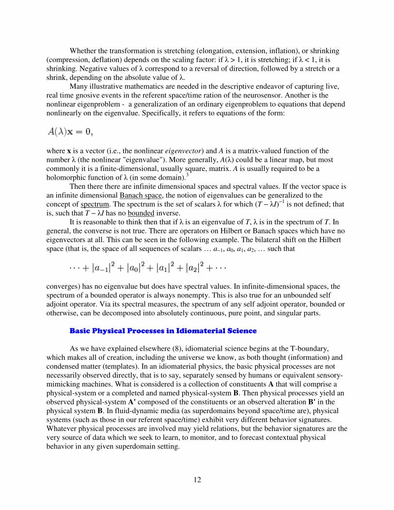
nonlinear eigenproblem - a generalization of an ordinary eigenproblem to equations that depend

nonlinearly on the eigenvalue. Specifically, it refers to equations of the form:

where x is a vector (i.e., the nonlinear eigenvector) and A is a matrix-valued function of the

number λ (the nonlinear "eigenvalue"). More generally, A(λ) could be a linear map, but most

commonly it is a finite-dimensional, usually square, matrix. A is usually required to be a

holomorphic function of λ (in some domain).3

Then there there are infinite dimensional spaces and spectral values. If the vector space is

an infinite dimensional Banach space, the notion of eigenvalues can be generalized to the

concept of spectrum. The spectrum is the set of scalars λ for which (T − λI)−1

is not defined; that

is, such that T − λI has no bounded inverse.

It is reasonable to think then that if λ is an eigenvalue of T, λ is in the spectrum of T. In

general, the converse is not true. There are operators on Hilbert or Banach spaces which have no

eigenvectors at all. This can be seen in the following example. The bilateral shift on the Hilbert

space (that is, the space of all sequences of scalars … a−1, a0, a1, a2, … such that

converges) has no eigenvalue but does have spectral values. In infinite-dimensional spaces, the

spectrum of a bounded operator is always nonempty. This is also true for an unbounded self

adjoint operator. Via its spectral measures, the spectrum of any self adjoint operator, bounded or

otherwise, can be decomposed into absolutely continuous, pure point, and singular parts.

Basic Physical Processes in Idiomaterial Science

As we have explained elsewhere (8), idiomaterial science begins at the T-boundary,

which makes all of creation, including the universe we know, as both thought (information) and

condensed matter (templates). In an idiomaterial physics, the basic physical processes are not

necessarily observed directly, that is to say, separately sensed by humans or equivalent sensory-

mimicking machines. What is considered is a collection of constituents A that will comprise a

physical-system or a completed and named physical-system B. Then physical processes yield an

observed physical-system A' composed of the constituents or an observed alteration B' in the

physical system B. In fluid-dynamic media (as superdomains beyond space/time are), physical

systems (such as those in our referent space/time) exhibit very different behavior signatures.

Whatever physical processes are involved may yield relations, but the behavior signatures are the

very source of data which we seek to learn, to monitor, and to forecast contextual physical

behavior in any given superdomain setting.

13

We cannot treat presumed physical laws thought to be valid in any one or another

superdomain environment, and thus we cannot treat anything yet as theory that can behave like a

black box which displays any given set of behavior parameters. There are no mathematical

expressions or discernible geometric figures embedded in the flows and eddies of the medium of

which superdomains are made. Everything is beyond form, and all lies in the idiomateriality of

information. Information in these media is beyond anything Shannon ever dream about. But

using mathematical logic, we are learning to model thought behavior (or behavior produced by

informatic interplay between aspects, sectors and domains) of various superdomains of the

Unum.

In quantum theory, hypothesized objects and processes can be characterized by

mathematical ideas, and from observable behavior, behavior signatures of these objects and

processes can be mathematically predicted. Methods of prediction include a combination of the

mathematics plus an interpretation and human logic which use the same or similar logic

modalities used in the mathematics themselves. This kind of interpretation then allows for a

replacement of the abstract mathematical terms for useful terms taken from a list of physical or

other discipline terms.

Finally, data comes to what one’s choice of virtual or undetectable physical object is

admitted as valid source. What is admitted as data depends on personal choice and prejudice,

training and predisposition. Nevertheless, those objects don’t have to correspond to reality

because there are other theories which, according to (9),few know about, that don't employ many

of them and that predict the same results using the same philosophy of science. More

importantly for what follows is that the philosophy can also be applied to gnosive notions and to

what is defined in life physics as not directly detectable idiomaterial stuff. This then makes the

following adaptation of Hermann’s immaterial and basic model scientific in character, and it

can't be rejected by mere or simple claims to the contrary. This, however, is also beyond the

scope of this short essay.

One more thing, though, before closing: the idea of the immaterial we use is quite distinct

from the defined objects used throughout the GGU-model ultranatural world. (9) defines the

ultranatural world as comprised of any mathematical representation for physical world entities as

well as others that form a not directly detectable background universe or substratum. The

operators used therein represent "physical-like" processes. Due to how the mathematics is

employed, technically, as operators, physical processes are members of the set of all ultranatural

processes. Operators within the ultranatural world represent physical-like processes in the same

manner that physical process relations are represented in the physical world except that the

physical-like processes are not members of the set of all physical processes.

NNOOTTEESS

1. In this regard, gnosive evidence we generated in the early years of the 2000-2010 decade

showed that matter generated at a formless boundary range (not singularity) we dubbed the T-

boundary was protocondensate thought behaving like protoparticulate matter would until it

reached a resonance superfunction in the resonant harmonics of the Unum we called unisonic

superdomain. Anything beyond the unisonic superfunction would then begin to demonstrate

functional characteristics of protoparticles agglutinating as protoparticulate matter. The process

is quite more complex, for which we then refer you to (4).

14

2. At the start of the 20th century, Hilbert studied the eigenvalues of integral operators by

viewing the operators as infinite matrices (7). He was the first to use the German word eigen to

denote eigenvalues and eigenvectors in 1904, though he may have been following a related usage

by Helmholtz. "Eigen" can be translated as "own", "peculiar to", "characteristic", or “individual,"

emphasizing how important eigenvalues are to defining the unique nature of a specific

transformation.

3. For example, an ordinary linear eigenproblem , where B is a square matrix,

corresponds to A(λ) = B − λI, where I is the identity matrix. One common case is where A is a

polynomial matrix, which is called a polynomial eigenvalue problem. In particular, the specific

case where the polynomial has degree two is called a quadratic eigenvalue problem, and can be

written in the form:

in terms of the constant square matrices A0,1,2. This can be converted into an ordinary linear

generalized eigenproblem of twice the size by defining a new vector . In terms of x and

y, the quadratic eigenvalue problem becomes:

where I is the identity matrix. More generally, if A is a matrix polynomial of degree d, then one

can convert the nonlinear eigenproblem into a linear (generalized) eigenproblem of d times the

size. Besides converting them to ordinary eigenproblems, which only works if A is polynomial,

there are other methods of solving nonlinear eigenproblems based on the Jacobi-Davidson

algorithm or based on Newton's method (related to inverse iteration).

RREEFFEERREENNCCEESS

1. Baez, J. C. & Stay, M. Physics, Topology, Logic and Computation: A Rosetta Stone. Narch

15, 2008.

2. Bordon, A. R. Ultimate causation (T-boundary) as causal sui-genesis of all superdomains,

including 4-spacetime. Foundation Reports in Life Physics 1, 1, 60-108, 2004(a).

3. Bordon, A. R. Ultimate causation (T-boundary) as causal sui-genesis of all superdomains,

including 4-spacetime. Foundation Reports in Life PhysicsFoundation Reports in Life PhysicsFoundation Reports in Life PhysicsFoundation Reports in Life Physics 1, 1, 60-108, 2004(b).

4. Joyal, A. and R. Street, The geometry of tensor calculus I, Adv. Math. 88 (1991), 55-113.

5. Yetter, D. N. Functorial Knot Theory: Categories of Tangles, Coherence, Categorical

Deformations, and Topological Invariants, World Scientific, Singapore, 2001.

6. Szabo, M . E., ed., Collected Papers of Gerhard Gentzen. North Holland, Amsterdam, 1969.

7. Cohen-Tannoudji, Claude. Quantum mechanics. New York, Wiley & Sons, 1977 (Chapter II.

The mathematical tools of quantum mechanics).

8. Bordon, A. R. & Wienz, E. M. How the Life Physics Group – California came about. LPG-

California, Los Angeles Hub, 2009.

9. Herrmann, R. A. Thought control: A rational model for immaterial mental influences.