NASA Technical Memorandum

ICOMP-94-22

106737 ?7-J£0

Boundary Conditions for UnsteadyCompressible Flows

S.I. Hariharan

Institute for Computational Mechanics in PropulsionLewis Research Center

Cleveland, Ohio

and The University of AkronAkron, Ohio

and

D.K. Johnson

The University of AkronAkron, Ohio

(NASA-TM-I06737) BOUNDARY

CONDITIONS FOR UNSTEADY

COMPRESSIBLE FLOWS (NASA.

Research Center) 2B p

Lewis

G3/}4

N95-12380

Unclas

0027030

Sep_mber 1994

National Aeronauticsand

Space Administration

https://ntrs.nasa.gov/search.jsp?R=19950005967 2018-06-17T07:06:58+00:00Z

BOUNDARY CONDITIONS FOR UNSTEADY COMPRESSIBLE FLOWS

S.I. Hariharan*

/nst/tute for Computational Mechanics in PropulsionLewis Research Center

Cleveland, Ohio 44135

and The University of Akron

Department of Mathematical SciencesAkron, Ohio 44325

D.K. Johnson

The University of Akron

Department of Mathematical SciencesAkron, Ohio 44325

Abstract

This paper explores solutions to the spherically symmetric Euler equations.

Motivated by the work of Hagstrom and Hariharan [7] and Geer and Pope [5],

we model the effect of a pulsating sphere in a compressible media. The literature

available on this suggests that an accurate numerical solution requires artificial

boundary conditions which simulate the propagation of nonlinear waves in open

domains. Until recently, the boundary conditions available are in general linear,

and based on non-reflection. Exceptions to this are the nonlinear non-reflective

conditions of Thompson [11], and the nonlinear reflective condition of [7]. The

former is based on the rate of change of the incoming characteristics, while the

latter relies on asymptotic analysis and the method of characteristics and accounts

for the coupling of incoming and outgoing characteristics. Furthermore in [7] it

was shown in a test situation in which the flow would reach a steady state over

a long time, the method proposed in [11] could lead to an incorrect steady state.

The current study considers periodic flows. Moreover, all possible types and

techniques of boundary conditions are included in this study. The technique

recommended by [7] proved superior to all others considered, and matched the

results of asymptotic methods which are valid for low subsonic Mach numbers.

*Supported in part by NSF Grant DMS-8921189, and by NASA cooperative

agreement NCC-3-104.

1 Introduction

This paper deals with an exterior problem governed by compressible, inviscid gas dynam-

ics equations. The nonlinear nature of the problem calls for a numerical solution to the

problem. As common to most exterior problems, the condition(s) that must be satisfied

at inf_ty is the key to solve these problems uniquely. The conditions that are physically

correct are not necessarily mathematically correct for the well-posed-ness of the problem.

Among the well known examples the one that stands out in the literature is the exterior

problem governed by the Helmholtz equation. The class of problems that is governed by

this equation include scattering of acoustic and electromagnetic waves. While physically,

the quantities decay to zero at in_quity, the requirement being exactly zero at infinity is

not a well posed condition, as observed by Hellwig (see reference[10]). The same holds

true for the Euler equations under consideration. Moreover, the computational consider-

ations require that these problems are to be solved in a finite domain with the aid of an

artificial boundary placed sufHciently far away from the region of local flows that are of

interest. This introduces another parameter L (eg. the radius of the artificial bounda-.-y)

and the requirement of boundary condition(s) that should be consistent with the true

inf_te domain problem. Several efforts have been marie along these lines. Most ei_orts

consider linearized flows (linearized about the state at in6nlty) to obtain such classes of

boundary conditions (For example see [2] and [6]). Among the first nonlinear versions of

the boundary conditions for gas dynamics problems was that of Hedstrom [9]. Recently

Thompson [11] extended the ideas of Hedstrom to multie]i,n_n_onal problems. His pro-

cedure works well for two dimensional problems described in Cartesian coordinates with

rectangular boundaries. Thompsons method works because in Cartesian coordinates the

flux term of the equation for the outgoing w_ve can be neglected. Although this technique

can be implemented in spherical and cylindrical coordinate systems, it will produce poor

results because the equations for the outward and inward propagating wave variables are

coupled in the flux term.

There is another parameter that is present in the computational model. This param-

eter is the total length of computational time, T. For problems that require long time

stability, such as the ones considered in this paper, the ideas of [3] cannot be used as

these are high frequency boundary conditions. They will be accurate for short times and

one cannot expect them to work well for any long time calculations.

Motivated by the work of Hagstrom and Hariharan [7] and the asymptotic work of

Geer and Pope [5] as well as Hardin and Pope [8], we model the external flow around a

sphere pulsating in the air. This problem is of considerable interest from a mathematical

2

standpoint as a testing ground for various versions of time dependant open boundary

conditions and asymptotic methods. Until recently, such boundary conditions have all

been linear, and based on non-reflection_ however for many problems such as the pulsating

sphere, or jet flow computations, the the nonlinearity is important, and the waves are

coupled such that an outward propagating wave will generate an inward travelling wave.

Exceptions to these kind of conditions are the technique of [7], which is a nonlinear

reflective condition that is based on asymptotic analysis, and the nonlinear non reflective

technique of Thompson [11]. This work applied the above methods to the case of fully

unsteady flow resulting from a pulsating sphere. Furthermore various other boundary

condRions were assessed along with the ones in [7] and [Ii].

2 Model and Derivation

Considering isentropic, compressible flow the Euler equations are given by

a p + V-(_) = 0, (1)0t

vp + p(!_ + (¢. v)_ = 0, (2)p = kf. (3)

Equations (1) and (2) are known as the conservation of mass and momentum equations,

and (3) is an isentropic constitutive l_w. Here p is density, _ is the velocity field vector,

p is pressure, t is time, and k and 7 are constants characteristic to the medium. The

model problem considered is the special case of a sphere harmonically ptdsating in a fluid

medium. Accordingly, the first assumption in this problem is that the flow is spherically

symmetric and the governing equations take the form

ap 0 2pu+ _(_) = , ,

__ o (p+p,,,) : 2_'(_)+ _ _ ,p = kf.

Then we scale the variables in the following manner:

(4)

p = po#, (7)

: u_, (8), = L#, (9)

t =(L/Co)i, (10)

where U, po, and L are a radial velocity, density, and length characteristic to the problem

and the local speed of sound of the medium is defined by

_' = _ = k-yf-' (11)Op

Co = C(po), (12)

with the Mach number given as M = U/co. This scaling along with lettingz = M_

and implementing (6) yield the followingnondimensionalized system

0p cgz -2z (13)aT+ o-7= T'

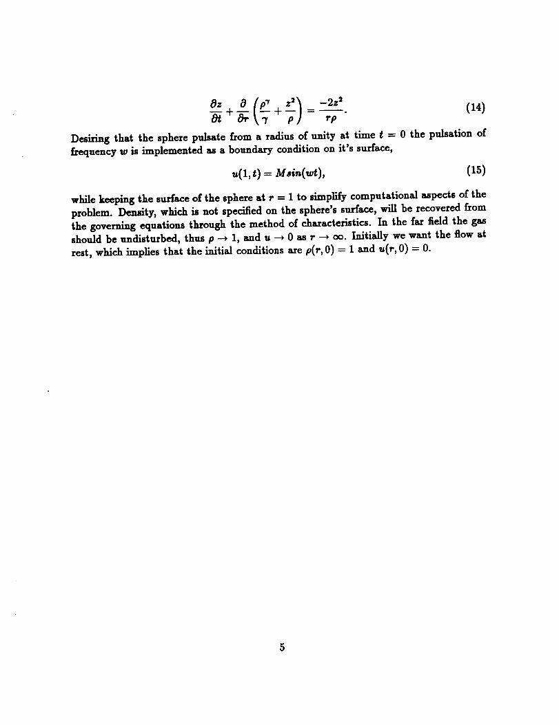
az a I_ _) -2z 2 (14)+ = ,pDesiring that the sphere pulsate from a radius of unity at time t -- 0 the pulsation of

frequency w is implemented as a boundary condition on it's surface,

u(1, t)- Msin(wt), (15)

while keeping the surface of the sphere at r = 1 to simplify computational aspects of the

problem. Density, which is not specified on the sphere's surface, will be recovered from

the governing equations through the method of characteristics. In the far field the gas

should be undisturbed, thus p --, i, and u --, 0 as r --* oo. Initially we want the flow at

rest, which implies that the initial conditions are p(r, 0) -- 1 and u(r, 0) = 0.

5

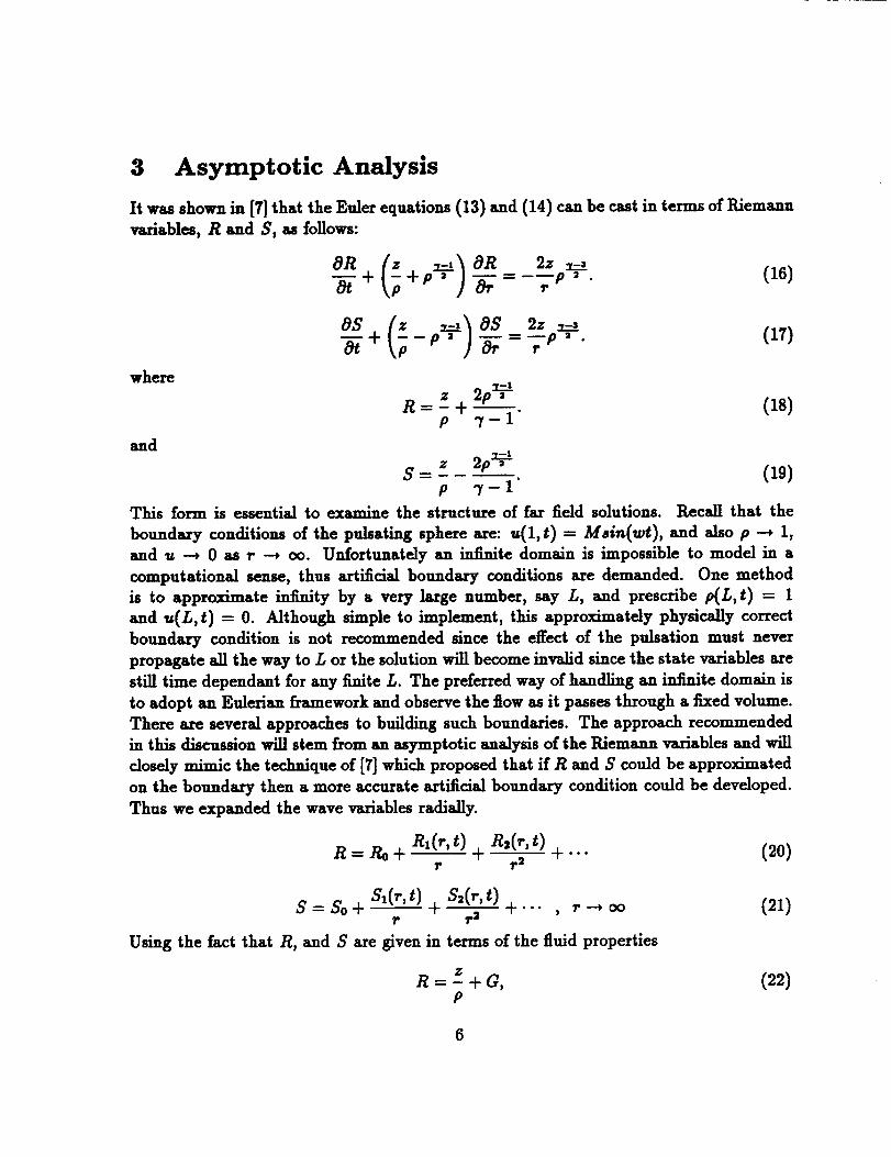
3 Asymptotic Analysis

It was shown in [7] that the Euler equations (131 and (141 can be cast in terms of Riemann

variables, R and 3, as follows:

where

and

R- z + --2P2_'_. (18)p 7-1

S-- z 2p_-_ (19)p "7-1"

This form is essential to examine the structure of far field solutions. Recall that the

boundary conditions of the pulsating sphere are: u(1,t) = Msin(_at), and also p -* 1,

and 1= --* 0 as r --, oo. Unfortunately an hifinite domain is impossible to model in a

computational sense, thus artificial boundary conditions are demanded. One method

is to approximate infinity by a very large number, say L, and prescribe p(L, t I = 1

and u(L, t ! = O. Although simple to implement, this approximately physically correct

boundary condition is not recommended since the effect of the pulsation must never

propagate all the way to L or the solution will become invalid since the state variables are

still time dependant for any finite L. The preferred way of handling an infinite domain is

to adopt an Eulerian framework and observe the flow as it passes through a fixed volume.

There are several approaches to building such boundaries. The approach recommended

in this discussion will stem from an asymptotic analysis of the Riemann variables and will

closely mimic the technique of [7] which proposed that if R and ,.q could be approximated

on the bounds, T then a more accurate artificial boundary condition could be developed.

Thus we expanded the wave variables radially.

/h(r,t)R- Ro + R1(r,t) + _ + ... (20)I" r 2

s,(,,t) s,(,,t)S=So+--+ +.-. , r--,co

/,, /,2

Using the fact that R, and S axe given in terms of the fluid properties

(21)

,¢R= -+G,

P(22)

6

ZS'- -- --G,

P

the values of Ro, and So come from direct application of the fax field data.

RO'-- _&"-- w

2

7-1

Then by substituting

andz R+S

p 2 '

the wave vaxJable equations assume the following form,

_-+ _+( ) _-= (R'-s'),

o-7+ 2 ( )Applying the asymptotic expansions

+

-_(R_/_+ R_/_' +...) +

+(7- i)12(Ro+ (R,- S,)I2,+ (R2+ S2)12,'+...)j-_(RII,+ ...)L= -,_,' (2(e,oR,- SOS,)/,+ (2RoR2+ _ - 2SOS,- S_)I; + ...),

mad,

+

o S_/,'_(s,/,+ +...)+[ oR,+s,)/_,+c_,+s,)/_,,+... 1_

(7- 1)/2(P,o+ (R, - s,)12, + (R, + s_)12,,+...) __ (s,/, +...)[= -=-_ (2(_R, - sos,)l, + (2_R, + PJ- 2SOS,- S_)l,, +...)

2r

we obtain the first order problem,

( R1 + $1 - R1 + $1 OR1

0S1 I R_ + $1

-_T + _ _, 7-1( R, + S, ) ) OS,2 _ + 2, -_r = o,

(23)

(24)

(25)

(26)

(2z)

(28)

(29)

(30)

(31)

(32)

7

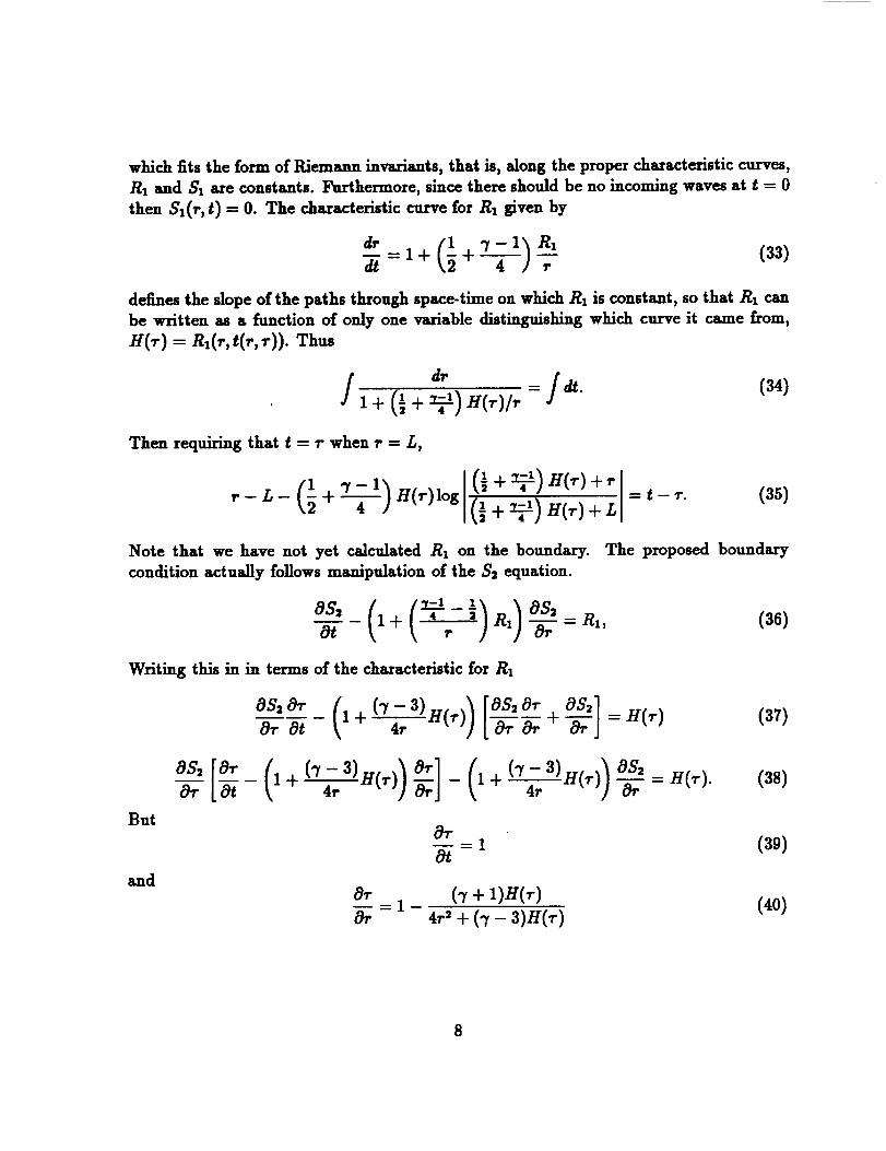
which fits the form of Riemann inva_uts, that is, along the proper characteristic curves,

Rx and $I are constants. Furthermore, since there should be no incoming waves at t = 0

then St(r, t) -" O. The characteristic curve for RI given by

= 1 + + --r (33)

defines the slope of the paths through space-time on which Rz is constant, so that Rx can

be written as a function of only one vm-isble distinguishing which curve it came from,

H(,') = R,C,-, t(,', ,')). Thus

/,+ (34)

Then requiring that t - _" when r = L,

r-/"- (2 + "_)H(r)log (__ + 4::_)H('r)+ L,= t- (35)

Note that we have not yet caJculsted Rz on the boundary. The proposed boundary

condition actually follows manipulation of the Sz equation.

1 + 4 1P -_1 --_ --- ,R1, (36)

Writing this in in terms of the characteristic for R,

@r Ot (1+ ('7_ 3)H("r))[._.__.S_ 0"ra_rr+ OS21=H(r)Orj (37)

But

and

aS, = H('r). (38)a,.S'2_[______(1-I--('7-3.---)H('r))4r _]-(1-I--('7_ 3)H('r))-_-

= 1 (39)

01" _ 1 (7 + 1)H(r) (40)Or 4r' + (7 - 3)H(_')

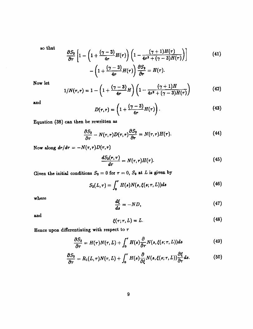
sothat

Now let

and

[1-(1+ 3)H0"))(1-4ri 3- (r)JJ(7+

(7 + 1)H

1/N(r,r) = 1-(1+ (7_r3)H) (1- 4,, .._ _,_'_-'_H(,r) j

Equation (38) can then be rewritten as

-- - N(,-,,.)D(,-,"1--_"os, = N(_,,-)Hff).OS_

_T

Now_o_ d,./d,-= -Nff,,)D(_,,)

dS,(,',,') = N(,-,,')_(,-).dr

Given the initial conditions ,5'2 = 0 for r = 0, $2 at L is given by

S2(L, r) = fo" H(s)N(s,_C(a; r,L))ds

whered_

- ND,d_

and

_(r;r,L) = L.

Hence upon differentiating with respect to T

f0 _ 0OS, _ H(r)N(r,L) + H(s)_-_rNCs,/_Cs;r,L))ds

0 rL O_dsOS2 = R_(L,r)NCr, L) + /o'H(s)_-_N(s,((s; , ))_-_ •

(41)

(42)

(43)

(44)

(45)

(46)

(47)

(48)

(49)

(50)

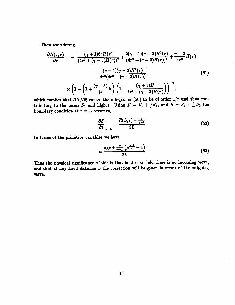
Then considering

oN(y,,) I" (_+ I)S,.H0-)= - L(4,':+ (_,- 3)H0"))'

2(7 - 1)(q - 3)H_(_ ") - s+

(4r' + (7 - 3)H(r))' + 4r 2 H(_')

(7 + 1)(7 - 3)H'(r) ]

(7 + 1)H 1 I-'

x (1-(1+ ('7_3'H)(1-4r,_-(_l'_--_-_H(Ir))) ,

(51)

which implies that aN/O_ causes the integral in (50) to be of order 1/r and thus con-

= ;'Rz, and S = So + _$2 thetributing to the terms Ss and higher. Using R Re + x

boundary condition at r : L becomes,

as] R(L,O '= ,-I (52)"_" :,. _'L

In terms of the primitive variables we have

zlP-l- _-_--f_1(p=_'31--1)

2L(53)

Thus the physical significance of this is that in the far field there is no incoming wave,

and that at any fixed distance L the correction will be given in terms of the outgoing

wave.

10

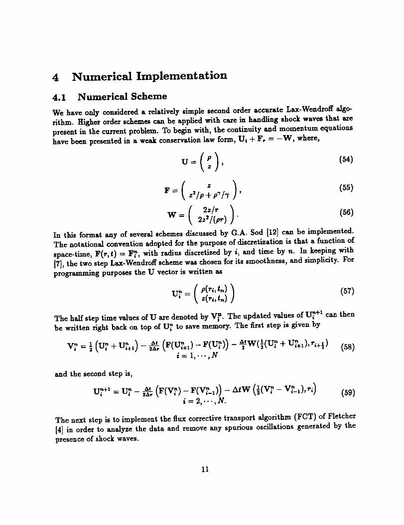
4 Numerical Implementation

4.1 Numerical Scheme

We have only considered a relatively simple second order accurate Lax-Wendroff algo-

rithm. Higher order schemes can be applied with care in handling shock waves that axe

present in the current problem. To begin with, the continuity and momentum equations

have been presented in a weak conservation law form, Ut ÷ F, - -W, where,

P= z2/O+f/_, ,

w = 2.'/[_) "

In this format any of several schemes discussed by G.A. Sod [12] can be implemented.

The notational convention adopted for the purpose of discretization is that a function of

space-time, F(r, t) - F_, with radius discretized by i, and time by n. In keeping with

[7], the two step Lax-Wendroff scheme was chosen for its smoothness, and simplicity. For

programming purposes the U vector is written as

U'_= ( p(vi'tn) ) (57)z(r,,t_)

The half step time values of U are denoted by V n. The updated values of U_i +1 can then

be written right back on top of U_ to save memory. The first step is given by

V_-- I (U_ -[- UinF1)- At _'_'-' +us_)"_+i) (58)i= 1,.-.,N

and the second step is,

1 n: -i-- 2,...,N.

(50)

The next step is to implement the flux corrective transport algorithm (FCT) of Fletcher

[4] in order to analyze the data and remove any spurious oscillations generated by the

presence of shock waves.

11

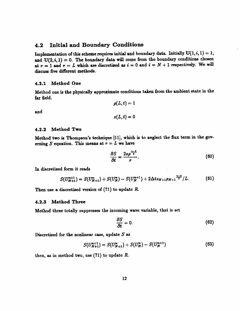
4.2 Initial and Boundary Conditions

Implementation of this scheme X_lUires initial and boundazy data. Initially U(1, i, 1) = 1,

and U(2, i, 1) - 0. The boundary data wig come from the boundaxy conditions chosenat r = 1 and r -- L which aze discretized as i = 0 and i = N + 1 respectively. We will

discuss five different methods.

4.2.1 Method One

Method one is the physically approximate conditions taken from the ambient state in the

far field.p(L,t) = 1

and•(L,t)= 0

4.2.2 Method Two

Method two is Thompson's technique [11], which is to neglect the flux term in the gov-

erning S equation. This means at r = L we have

In discretized form it reads

08 2zp_, "

Ot r

H(_++_) = H(_+z) -t- S(_) - H(_ +z) -t- 2_tzN+zpN+z = IL.

Then use a discretized version of (71) to update R.

(60)

(61)

4.2.3 Method Three

Method three totally suppresses the incoming wave vaxiable, that is set

0S--=0.0t

Discretized for the nonline_ case, update 5' as

= + - +')

then, as in method two, use (71) to update R.

(62)

(63)

12

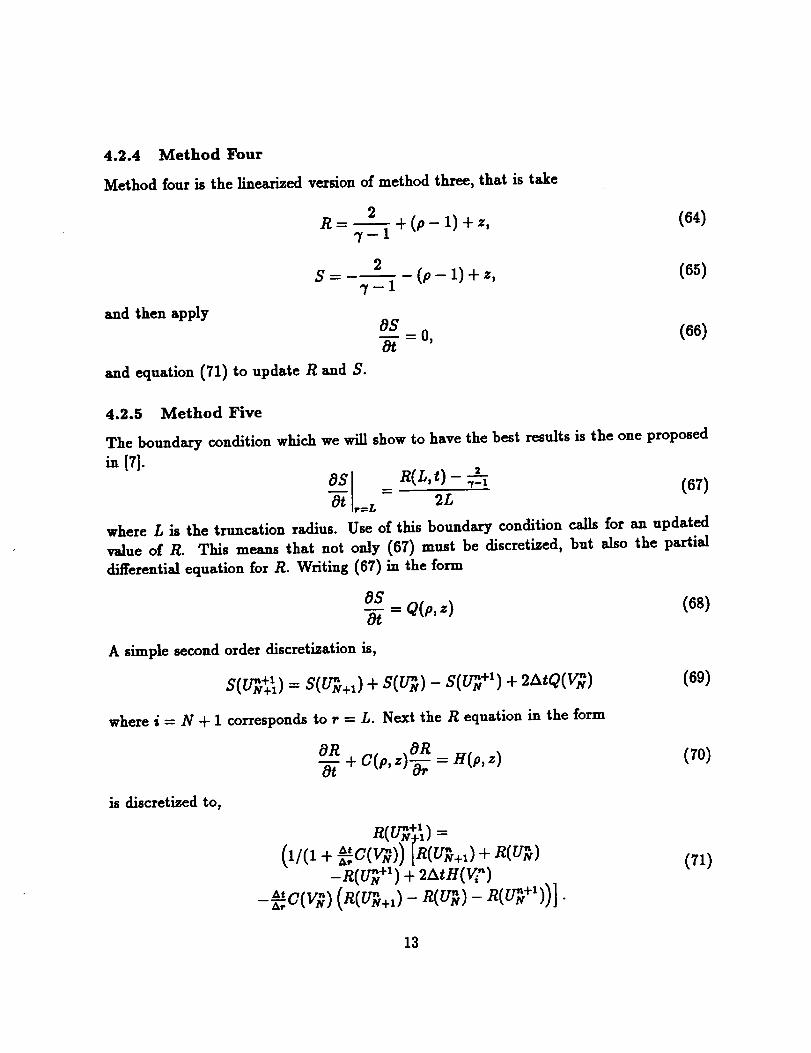
4.2.4 Method Four

Method four is the linearized version of method three, that is take

2R=--+(p- Z)+z,

_/-1

and then apply

2S- (p- 1)+z,

"y-1

(64)

and equation (71) to update R and 5'.

(65)

OE-_ = o, (66)

4.2.5 Method Five

The boundary condition which we will show to have the best results is the one proposed

in [7]

O=qI R( L,t) == ,,-1 (61')"_",.=L _-L

where L is the truncation radius. Use of this boundary condition calls for an updated

value of R. This means that not only (67) must be discretized, but also the partial

differential equation for R. Writing (67) in the form

0$= O(p,z) (6s)

A simple second order discretization is,

S(_) = S(_+,) + S(_) - S(_ +') + 2Z_tQ(_) (69)

where i = N + 1 corresponds to r = L. Next the R equation in the form

is discretized to,

T7 + c(p,z) = H(p,,)

+1R(_+,) =_' " " R(_)(,/(1+

-R(_ +') + 2AtH(V,")/,t C,,V_ _ _ _ .,

(70)

(71)

13

Then the primitive v_ables canbeupdatedat the boundary usingthe updatedboundaryvaluesof R and S with ,

))-p- R- S "-', (72)

(73)z(R+s)z=_ p.

14

5 Results and Comparisons

As mentioned earlier, the governing equations were disc_etized using the two step Lax-

Wendroff scheme. All numerical tests were conducted with the surface of the sphere

pulsating with radial velocity u = Msin(wt) where w = 1.5, and the Mach number set

at, M = 0.5. The tests were designed to produce radial density and momentum profiles

at time value t = 10. Initially we ran tests using a computational domain that was larger

than the radius of propagation. This guaranteed that we had a solution that was inde-

pendent of any boundary conditions. With a Math number of M = 0.5 Gibbs phenomena

became visible near the shock waves, displaying highly oscillatory behavior. A flux cor-

rective transport subroutine by Fletcher [4] was employed to help capture the shocks and

mi_ oscillations as they occurred. To reassure the validity of the numerical solution

it was necessary to compare it with a completely independent method. Asymptotics are

often considered as _ltematives to numerical solutions. Asymptotic solutions use the

Mach as a parameter of expansion, thus requiring very low Math numbers. The multiple

scales technique of Geer and Pope [5] was chosen to compare with method one. Their

first order approximation for velocity is given as

(,- 1 +11,')sinO-)= (] cosO-)+ (1+ (74)

and the second order correction is given as

,,l(r,t) = (b_i,_+ 2_,1,)cos(2,.) + (b_l, _ - 2b_,l,)sin(_.,)

where

and

( (29 - 3"y)w _ w2Cw 2 - 1) ) (1 + "y)w_ log(r)+ _l_rS_+z0n)2 +r_C1+w2)2 cos(2r)- 4r2(1+w2)

_t_((29 - 3"y)w( w2-1 ) 2wS )32rs(1 + w') 2 - r2(1 + w')' sin(21")

f(t) = (sinC,.t)- ,.cosC,.t)l (1 + w')

_' = ¢ + (._+ 1)M(, - 1)f(t + 1- ,_)

_" - w(t + 1 - 11)

= _ 3w'(14 - 2'7 + 17w: + "/w:)16(1 + w')'(1 + 4w 2)

bs = w(29 - 3"y - 17w 2 + 15_w _ - 64w 4)32(1 + w2)2(1 + 4w'-)

(75)

(76)

(77)

(78)

(79)

(80)

15

Then the velocity is calculated as

uC,,t)= + (81)

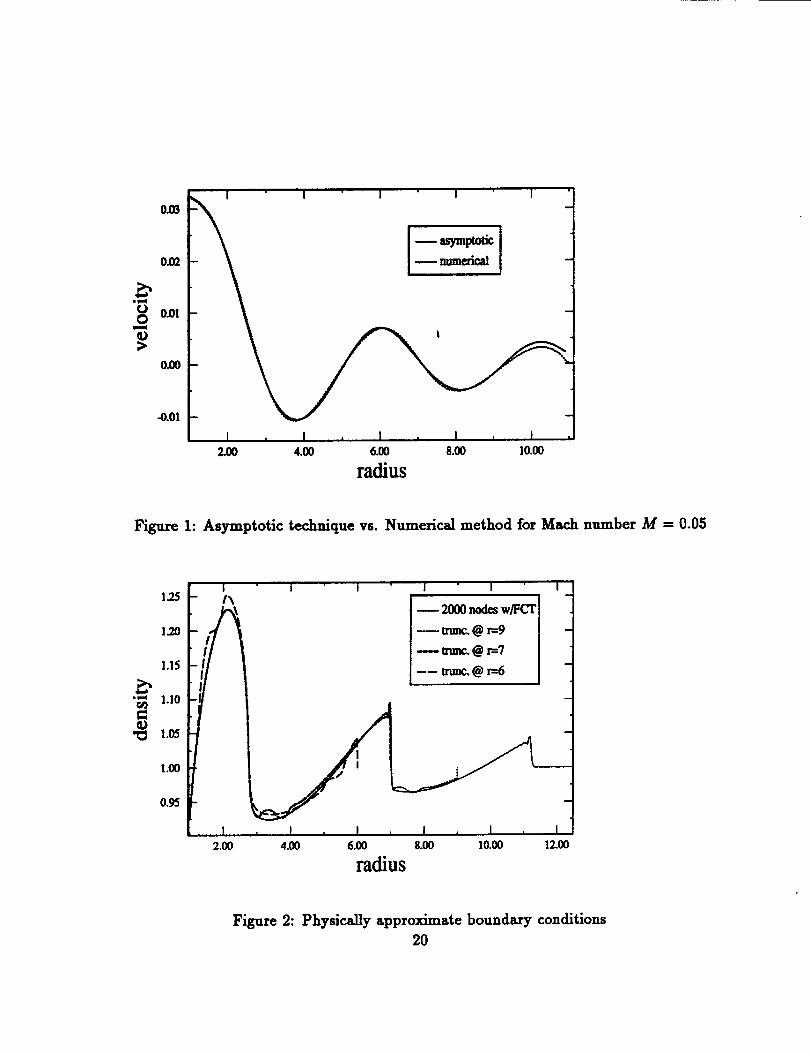
Figure 1 shows a velocity profile of [5] compared with the numerical method at time,

t = 10, generated with Math number, M = 0.05. These solutions agree fairly closely.

If an artificial boundary was placed at a radius where waves would pass through it

by time t = 10 then the effect of the artificial boundary conditions could be evaluated

by comparing it to the profiles calculated in a large domain which was independent of

boundary conditions. A perfect boundary condition would yield a profile that perfectly

matched these examples regardless of where the radius was truncated. In figure 2 the

physically approximate boundary conditions of method one were evaluated at r = 6,

r = 7, and r = 9. Figure 2 clearly shows that this physical approximation is invalid for

truncations inside of the radius of propagation.

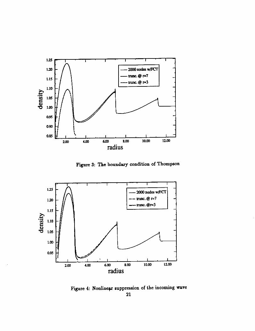
In figure 3 Thompsons method [11], method two, has been run at three different

truncation radii, L = 21 (L = 21 corresponds to 2000 nodes.), L = 7, and L - 3. If the

method two boundary condition was numerically correct, the profiles for L = 7, and L = 3

should virtually coincide with the profile for L = 21. Thompson's boundary condition

has caused the numerical scheme to undershoot the L = 21 profile when truncated at

L = 3, this is because Thompsons boundary condition will go to zero in the far field

independent of the behavior of the density.

The results of method three, the nonlinear suppression of the incoming wave, also

truncated at L = 21, L = 7, and L = 3, are given in figure 4. The basic difficulty is

the fact that even though this method was based on the Riemann variables, it did not

simulate the movement of the waves because it did not exploit the governing equations

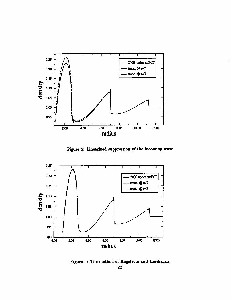
ofthe ables (16)and(17).Figure 5 presents the results of method four, the linearized suppression of the incoming

wave, when truncated at L = 21, L = 7, and L = 3 as in the previous tests. Although

not perfect, this technique does not perform badly for ten time units. The amplitude of

overshoot from the L = 3 truncation indicates that this method will not stay stable in a

far time application. Thus as time is increased the profile would continue to deviate.

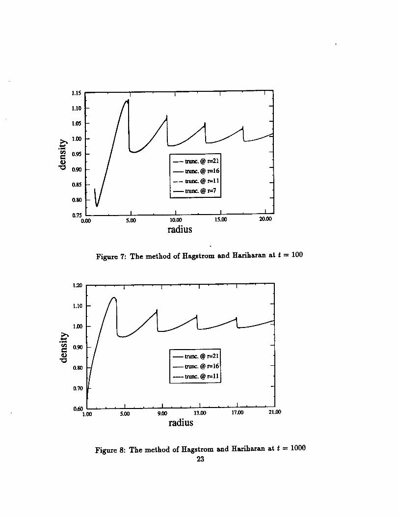
The results of the technique proposed in [7], method five, as shown in figures 6, 7,

and 8, are far superior to the other four methods which offer no hope for solutions in

long time calculations . In figure 6 the profiles generated with truncations at L = 3 and

L = 7 lay precisely on the profile of truncation at L = 21. This same style test was then

performed on method five at time t = 100 and t = 1000 (one ml]llon time steps) to see if

it would remain stable for a far time situation. In figures 7 and 8 the truncated profiles

continue to coincide, indicating that this technique precisely simulates waves passing the

artificial boundary and is dependable regardless of the time value to which the scheme is

run.

16

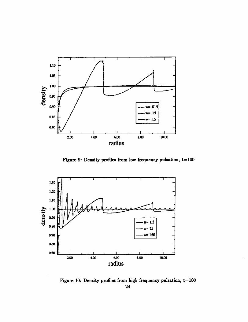
It is useful to examine the nature of the solutions as w --, 0 and as w --_ oo. As

one would expect, the variation of the solution in the computational domain are small

for low frequencies. Figure 9 shows this for decreasing values of u_ using method five.

(In this case the nonlinear effects are more prominent in the far field than in the near

field.) On the other hand for high frequency waves an increase in the frequency reflects

more periodic structures of the shock waves. Figure 10 shows a tenfold increase in the

number of shock fronts by going from w = 1.5 to w = 15. However further increase

in the frequency poses a challenge for the numerical computations. As the frequency

increases the fronts are closer to each other. In the extreme cases one must develop an

asymptotic solution to these problems. For example figure 10 suggests that the solution

rapidly attenuates for w = 150. These asymptotic aspects require further study.

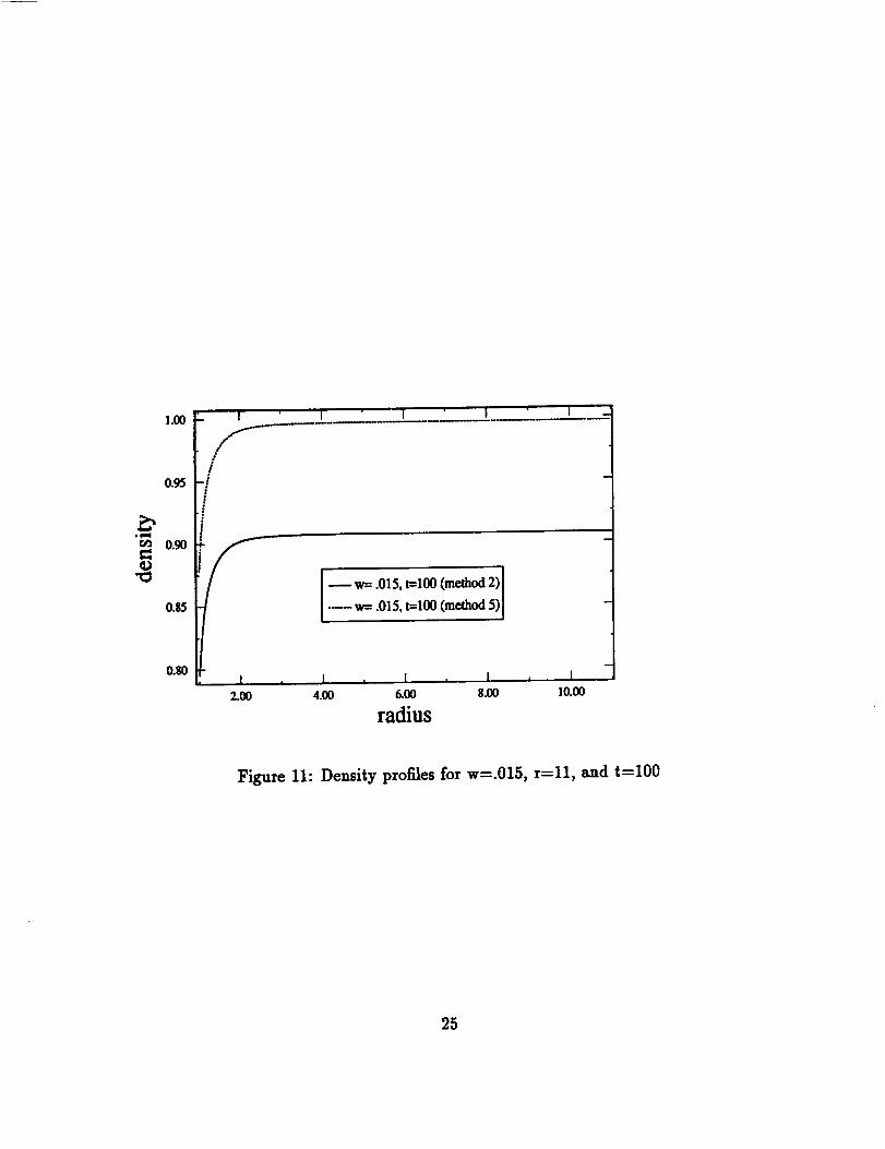
Considering figure 9, method five works quite we]] for low frequency problems, but

this was not the case for all other classes of boundary conditions. In figure ll we show

the solution of Thompson for w = .015, with L = 11 and t = 100. For t = 100 the

sphere will not have gone through a full oscillation, but the wave will have passed our

truncation point at L = ll. This solution approaches an incorrect state well below what

would be expected (compare with figure 9), Thus it is not uniformly accurate in time.

The method proposed in [7] is indeed a uniformly valid condition due to its derivation

that is based on uniform asymptotic expemsions.

17

6 Conclusion

This paper has modeled the flow field generated by a pulsating sphere. This model-

ing process involved exploring the laws of gas dynamics and combining these laws with

mathematical analysis in order to obtain numerical solutions for the flow field. Because

of the intrinsic spherical symmetry of the problem the solutions naturally took the form

of radial density and velocity profiles for specified times of interest. The numerical ira-

plementation of the governing equations was of particular mathematical interest because

it became necessary to include a flux corrective transport algorithm to help control the

numerical instabilities generated by the presence of shock waves.

The next topic to be addressed in the modeling process was to come up with suitable

numerics] boundary conditions. Following the lead of Hagstrom and Hariharan [7] a

method of characteristics representation was created to sense the presence of incoming

and outgoing waves, and then implemented as a numerical boundary condition. The

boundary condition was then evaluated along with several other techniques for stability

far in time, and consistency regardless of the radius at which the domain was truncated.

This discussion revealed that for the numerical solution of problems in gas dynamics the

modeling of the open boundary conditions is critical. The wrong form of these conditions,

especia/]y in fuXly unsteady flow, can lead to a completely incorrect solution. Yet from

all this, the technique of [7] has proven to be a dependable method for problems that

can be modeled as having spherical wavefronts in the far field. Future work in this field

is the generalized boundaxy condition for frilly three dimensional unsteady flow.

References

[1] M.B. Abbot, An Introduction To The Method of Characteristics, Thames and Hud-

son, 1966.

[2] A. Bayliss, E. Turkel, Far field boundary conditions for compressible flows, J. Comp.

Phys., 1982, 48, 182-199.

[3] B. Enquist, A. Majda, Absorbin9 boundary conditions for the numerical simulation

of waves, Math. Comp., 1977, 31, 629-651.

[4] C.A.J. Fletcher, Computational Techniques for Fluid Dynamics, Vol. II, Springer-

Verlag, 1988

[5] J. Geer, D. Pope, A Multiple Scales Approach to Sound Generation by Vibrating

Bodies, ICASE Report No. 92-73, 1992.

18

[6] B. Gustagsson, Far field boundary conditions for time dependant hyperbolic systems,

SIAM J. Sci. Star. Comp., 1988, 9, 812-828.

[7] T. Hagstrom, S.I. Harihaxem, Accurate Boundary Conditions for Ezterior Problems

in Gas Dynamics, Mathematics of Computation, Vol.51,No.184, Oct. 1988.

[8] J.C. Hardin, D.S. Pope, A New Technique for Aerodynamic Noise Calculation,

DGLR/AIAA 92-02-076.

[9] G. W. Hedstrom, J. Comp. Phys., 1979, 30,222

[10] G. Hellwig, Partial differential equations, Blaisdell, Waltham, Mass., 1964.

[11] K. Thompson, Time Dependant Boundary Conditions for Hyperbolic Systems, Jour-

nal of Computational Physics, Vol.68, No.l, 1987.

[12] G. Sod, A Survey of Several Finite Difference Methods for Systems of Nonlinear

Hyperbolic Conservation Laws, Journal of Computational Physics 27, 1-31 (1978).

19

0..08

0.02

_'_ 0.01

0.00

4).01

Figure 1: Asymptotic technique vs. Numerical method for Mach number M = 0.05

125

1.20

1.15

°_ 1.10

"_ 1._

1.00

0.95

I i i I I I

.d _ l_m_.@ _9 I

I/ X I

1 , I , I , I , I , I2.00 4.00 6.00 8.00 10.00 12.00

radius

Figure 2: Physically approximate boundary conditions20

1.2_

1.20

1.15

1.05

0._

0.90

0.85

/

lj!J

/II

I I I I

--2ooon_w_"I_tnmc.@ r=7 I

_ mmc.@ r=3 I

I

k, I , I , I , I , I

4.00 6.00 8.00 !0.00 12.00

radius

Figure 3: The boundaxy condition of Thompson

O

1.25

1_0

1.15

1.10

1.05

1.00

0.95

I

/7//7

I I I I

2000 nodes w/FCT I

___@__7 Ithroe. @r=-3 I

, I , I , I , I ,4.00 6.00 8.00 10.00

radius

I12.00

Figure 4: Nonline_ suppression of the incoming wave

21

1.25

1.20

1.15

1.10

1.OO

0.95

I

//#II

m

1

I I

i I Iuuac.@ _7 /

u'_.@ _3 /

, I , I , I , I , I4.oo 6.oo 8.oo 10.oo 12.oo

radius

Figure 5: Linesrized suppression of the incoming wave

1.20 -

1.15 -

J

1.oo -

0.95 -

0.90 -0.OO

,_ 1.10,¢.,_

r_

1.05

, I2.OO

I I I I I

-- 2000 nodes wlFCr II

--mmc.@ r=-7 l

--mmc.@ r=3 l

, I , I , I , I , I4.OO 6.OO 8.00 10.00 12.00

radius

Figure 6: The method of Hagstrom and Harihsran

22

1,15

1.10

1.05

1.00

0.95

'_ 0.90

0.85

0.80

0.750.00

I I I

_ , I , I o I , I_5.00 10.00 15.00 20.00

radius

Figure 7: The method of Hagstrom and Hariharan at t = 100

**,,4

r_

O

1_0

1.10

1.00

0.90

0.80

0.70

0.601.00

I I I I

, , I . , , I . . I , . , I , ,

5.00 9.00 13.00 17.00 21.00

radius

Figure 8: The method of Hagstrom and Hariharan at t = 1000

23

1.10

1.0_

g 1.00

0.95

'_ 0.90

0.85

0.80

I

!!

I I I

/

/ I , I

2.00 4.00

I

I--w=-ol5 I

--.w=.15

--w=l.5

, i , i , i

6.00 8.00 10.00

radius

Figure 9: Density profiles from low frequency pulsation, t=100

1.30

1.70

1.I0

1.000.90

'_ 0.80

0.70

0.60

O.5O

I i

I , I , I , I , I -2.00 4.00 6.00 8.00 10.00

radius

Figure 10: Density profiles from high frequency pulsation, t=100

24

r_

1.00

0.95

0.90

0.85

0.80

SI

-!i

i

I I I I -

w= .015, t=-100 (method 2)[

•--- w=- .015, t=100 (method 5>j

I , I , 1 , I , I

2.00 4.00 6.00 8.00 10.00

radius

Figure 11: Density profiles for w=.015, r=11, and t=100

25

Form Ap/_'orodREPORT DOCUMENTATION PAGE OMBNo.07040188

Pub4icraportingburd.enfor this collectionof infon'r_ion is astimated, to avorage 1 I'_Jr per response.,includingthe time for reviewinginstructions,seamhing existing data soumes,gathenng _ maJrttaimr_the _ rmeded.,and co._.=ng .andrev_lwmgthe .o.o1..lectmnof Informal=on.Send _commentsregardingthis burden estimateor any =her aspect of thiscollectionof anfonTk'dmn,nncludmg suggastm¢rs1orreduQng this burden, to WashingtonHeadquarters ServKms,Directoratefor InformationOperations and Reports, 1215 JollersonDavis Highway,Suite 1204, Adington.VA 22202-4302, and to the Office of Management and Budget,Paperwork ReductionProject (0704-0188), Washington. DC 20503.

1. AGENCY USE ONLY (Leave blank)

4. TITLE AND SUBTITLE

2. REPORT DATE

September 1994

Boundary Conditions for Unsteady Compressible Flows

6. AUTHOR(S)

S.I. Hariharan and D.K. Johnson

7. PERFORMINGORGANIZATIONNAME(S)AND ADDRESS{ES)

National Aeronautics and Space AdministrationLewis Research Center

Cleveland, Ohio 44135-3191

9. SPONSORING/MONITORINGAGENCYNAME(S)ANDADDRESS(ES)

National Aeronautics and Space Administration

Washington, D.C. 20546-0001

3. REPORT TYPE AND DATES COVERED

Technical Memorandum

5. FUNDING NUMBERS

WU-505-90-5K

8. PERFORMING ORGANIZATIONREPORT NUMBER

E-9138

10. SPO NSORINGAMON ITOPJ NG

AGENCY REPORT NUMBER

NASA TM- 106737ICOMP-94--22

11. SUPPLEMENTARY NOTES

S.I. Hariharan, Institute for Computational Mechanics in Propulsion, NASA Lewis Research Center, (work funded under NASA Cooperative Agreement

NCC3-233 and supported in part by NSF Grant DMS-8921189 and NASA Cooperative Agreement NCC3-104), and the University of Akron, Akron,

Ohio 44325; D. K. Johnson, the University of Akron, Akron, Ohio 44325. ICOMP Program Director, Louis A. Povinelli, organization code 2600, (216)433-5818.

12a. DISTRIBUTION/AVAILABILITY STATEMENT

Unclassified - Unlimited

Subject Category 34

12b. DISTRIBUTION CODE

13. ABSTRACT (Maximum 200 words)

This paper explores solutions to the spherically symmetric Euler equations. Motivated by the work of Hagstrom and Hariharan andGeer and Pope, we modeled the effect of a pulsating sphere in a compressible medium. The literature available on this suggests that anaccurate numerical solution requires artificial boundary conditions which simulate the propagation of nonlinear waves in open domains.Until recently, the boundary conditions available were in general linear and based on nortreflection. Exceptions to this are the nonlinearnonreflective conditions of Thompson, and the nonlinear reflective conditions of Hagstrom and Hariharan. The former are based on therate of change of the incoming characteristics; the latter rely on asymptotic analysis and the method of characteristics and account forthe coupling of incoming and outgoing characteristics. Furthermore, Hagstrom and Hariharan have shown that, in a test situation inwhich the flow would reach a steady state over a long time, Thompson's method could lead to an incorrect steady state. The eta'rent

study considers periodic flows and includes all possible types and techniques of boundary conditions. The technique recommended byHagstrom and Hariharan proved superior to all others considered and matched the results of asymptotic methods that are valid for lowsubsonic Mach numbers.

14. SUBJECTTERMS

Unsteady flow; Boundary conditions

17. SECURITY CLASSIFICATIONOF REPORT

Unclassified

18. SECURITY CLASSIFICATIONOF THIS PAGE

Unclassified

NSN 7540-01-280-5500

19. SECURITY CLASSIFICATIONOF ABSTRACT

Unclassified

15. NUMBER OF PAGES

2716. PRICE CODE

A03

20. LIMITATION OF ABSTRACT

Standard Form 298 (Rev. 2-89)

Prescribed by ANSI Std. Z39-18298-102