Computers and Geotechnics 71 (2016) 136–146

Contents lists available at ScienceDirect

Computers and Geotechnics

journal homepage: www.elsevier .com/ locate/compgeo

Boundary effects on the Soil Water Characteristic Curves obtainedfrom lattice Boltzmann simulations

http://dx.doi.org/10.1016/j.compgeo.2015.09.0080266-352X/� 2015 Elsevier Ltd. All rights reserved.

⇑ Corresponding author at: Research Group on Complex Processes inGeo-Systems, School of Civil Engineering, The University of Queensland, Brisbane,QLD 4072, Australia.

E-mail address: s.galindotorres@uq.edu.au (S.A. Galindo-Torres).

S.A. Galindo-Torres a,b,⇑, A. Scheuermann a,b, L. Li b

aGeotechnical Engineering Centre, School of Civil Engineering, The University of Queensland, Brisbane, QLD 4072, AustraliabResearch Group on Complex Processes in Geo-Systems, School of Civil Engineering, The University of Queensland, Brisbane, QLD 4072, Australia

a r t i c l e i n f o

Article history:Received 30 June 2015Received in revised form 18 August 2015Accepted 18 September 2015

Keywords:Lattice Boltzmann MethodsUnsaturated soil physics

a b s t r a c t

Pore-scale simulations using a Lattice Boltzmann Method (LBM)-based numerical model were conductedto examine how the capillary pressure ðPcÞ and saturation (S) evolve within a virtual porous mediumsubjected to drainage and imbibition cycles. The results show the presence of a sharp front (interfaceseparating the wetting and non-wetting fluids) across the cell during the test, which expectably movesup and down as the controlling non-wetting fluid pressure at the upper boundary varies to simulatedifferent Pc levels over the drainage and imbibition cycle. This phenomenon, representing inhomogeneityat the simulated scale, is in conflict with the homogenization applied to the pressure cell for deriving theconstitutive Pc—S relationship. Different boundary conditions, adopted to achieve more homogeneousstates in the virtual soil, resulted in different Pc—S curves. No unique relationship between Pc and S, evenwith the interfacial area ðAnwÞ included, could be found. This study shows dependence of theLBM-predicted Pc—S relation on the chosen boundary conditions. This effect should be taken into accountin future numerical studies of multiphase flow within porous media.

� 2015 Elsevier Ltd. All rights reserved.

1. Introduction

The Lattice Boltzmann Method (LBM) is growing in popularityfor simulations of complex multiphase systems involving fluids.Since the method is based on the Boltzmann equation instead ofthe traditional Navier Stokes equations, it is easier to include mod-els representing processes and effects at even the molecular scalesuch as those producing phase separation and immiscibility. Oneof the most popular models to reproduce the phase separation isby Shan and Chen (SC model) [1]. In this model, the molecularforces are included at a mesoscale by taking the average of theseforces over large assemblies of particles.

The SC model has been tested with experimental data bySchaap et al. [2]. In this work, a small sub volume was simulatedmainly because of the well-known, large computational intensityof the LBM. The results showed a remarkable agreement betweenthe LBM simulations and experimental data with only minimalcalibration efforts on the surface tension parameters. The pressuresof the different phases were controlled by fixing the density ofthe components at opposite sides of the domain. Such boundary

conditions have been used afterwards in similar modelling studies(e.g., [3]). These works show that in LBM-SC simulations there isusually a front connected to the injection point of either phase.During imbibition the wetting phase invades the porous mediaby this front followed by pockets of fluid broken from it duringdrainage. During the next imbibition cycle, these pockets becomeconnected to the front again.

The question remains whether the close link of the wetting frontto the boundary conditions is a realistic feature reproduced by theLBM-SC or it is an artefact of the method. To address this question,we present here results from extensive simulations carried out toexplore the dependence of the Soil Water Characteristic Curves(SWCC) simulated by the LBM-SC model on the choice of boundaryconditions. The analysis focuses on the relationship between thecapillary pressure ðPcÞ and saturation (S) of wetting fluid but alsoinvolves a third variable, the interfacial area ðAnwÞ between thewet-ting and non-wetting phases. Hassanizadeh and Gray [4] analysedthe multiphase porous media flow system and derived a multivari-ate relation among the three variables: Anw; Pc and S. The hystereticcycles shown in the Pc—S curves could then be explained as projec-tions of the Pc—S—Anw relation, which forms a new basis for the con-stitutive soil water retention characteristic. Various studies havebeen carried out to validate this multivariate relation using predic-tions by pore-network models [5] and LBM models [3] as well asmeasurements from laboratory experiments [6].

S.A. Galindo-Torres et al. / Computers and Geotechnics 71 (2016) 136–146 137

The paper is divided as follows: Section 2 explains the details ofthe LBM-SC implementation used for this study. Section 3describes how the key variables used in the analysis are deter-mined from the simulation results. The analyses for different con-figurations of boundary conditions are given in Section 4 followedby the discussions and conclusions in Section 5.

2. Model

For the simulations that were carried out, the LBM D3Q15scheme [7] was chosen. In this formalism the space is divided ina cubic grid. In order to solve the Boltzmann equation, further dis-cretization is needed in the velocity domain. For each cell, a set of15 discrete velocities (Fig. 1) are assigned and a probability func-tion f i is associated with each velocity. The velocities have indexesgoing from 0 to 14 with the first being the rest case with null veloc-ity. As an example the ~e14 discrete velocity is the vector Cð1;1;1Þ,where C is a lattice constant given by C ¼ dx=dt with dt being thetime step and dx the side length of each square cell. To define thefluid velocity~u and density q at a given cell, the following relationsare applied:

q ¼X14i¼0

f i

~u ¼X14i¼0

f i~ei

ð1Þ

It is also important to set a weight xi for each direction. For theD3Q15 scheme the weights are given as follows:

x0 ¼ 29;

xi¼1�6 ¼ 19;

xi¼7�14 ¼ 172

:

ð2Þ

After the velocities are defined, an evolution rule is imple-mented to solve the Boltzmman equation [8]:

f ið~xþ~ei; t þ dtÞ ¼ f ið~x; tÞ þXcol; ð3Þwhere ~x is the position of the given cell, t is the current time stepandXcol is an operator accounting for the collision of all the particlesthat exist within the cell. For this study, the widely accepted BGKmodel for the collision operator [9] was used, which assumes that

xy

z

e1

e2

e3

e4

e5

e6

e7

e8

e9

e10

e11

e12e13

e14

Fig. 1. LBM cell of the D3Q15 showing the direction for each of the 15 discretevelocities.

the collision processes drive the system into an equilibrium statedescribed by an equilibrium function f eqi ,

Xcol ¼ f eqi � f is

ð4Þ

where s is a characteristic relaxation time. Further research hasdemonstrated that the Navier Stokes equations for fluid flow [10]are recovered if,

f eqi ¼ xiq 1þ 3~ei �~uC2 þ 9ð~ei �~uÞ2

2C4 � 3u2

2C2

!ð5Þ

and the dynamic viscosity of the fluid m is given by,

m ¼ ðs� 0:5Þ d2x3dt

: ð6Þ

Eq. (6) imposes a constraint on the choice of s, which must begreater than 0.5 for the viscosity to be physically correct. It has beenknown that values close to 0.5 produce unstable numerical beha-viour [8]; hence it is always advisable to keep its value close to one.

In order to simulate multicomponent and multiphase flows aswell as body forces like gravity [11], a net force is introduced

for each cell. The net force ~F modifies the velocity used in thecalculation of the equilibrium function according to,

~u0 ¼ ~uþ dt~Fq

: ð7Þ

In the case of gravity, the force is simply~Fg ¼ q~g where~g is a vectorrepresenting the direction of the gravitational acceleration. Severalcomponents can also be simulated by assigning an independentlattice to each of them [12]. Then both fluid (lattices) interact by

way of repulsive forces ~Fr ,

~Fr ¼ �Grq1ð~xÞX14i¼1

xiq2ð~xþ dt~eiÞ~ei; ð8Þ

where Gr controls the repulsion intensity. With multiplecomponents considered, the equilibrium velocity (Eq. (1)) must becorrected by,

~u ¼P

rP14

i¼11sr f

riP

rqrsr

ð9Þ

where the contribution of each component r is accounted for [12].The interaction of the fluids with solids is twofold. The fluids

must be repelled by solid cells. Hence, the bounce-back boundarycondition [8] is implemented for cells that are tagged as solids.In the bounce-back condition, after the collision step, the distribu-tion functions are swapped symmetrically as,

f�i ¼ f i ð10Þwhere the subscript �i refers to the opposite direction to the ithvelocity. However, to model capillarity effects, the fluid should alsobe attracted to the solid in a similar way as described in Eq. (8),

~Fa ¼ �Gsqð~xÞX14i¼1

xisð~xþ dt~eiÞ~ei; ð11Þ

where Gs controls the intensity of the fluid–solid attraction and thefunction s is unity when the neighbouring cell is tagged as solid andzero otherwise. Through parameters Gr and Gs, important quantitiessuch as the contact angle, surface tension and immiscibility ofmultiple components, can be controlled. For instance the contactangle h can be shown to follow [3],

cos h ¼ G1s � G2

s

Grð12Þ

where the superscripts indicate the different fluids.

Table 1Parameters values used in the simulations.

Parameter Value

dx 10�4 ms 1.1Gr 1.0Gs �0.5a

q0, equilibrium density for both fluids 1.0 g/cm3

rp 0.028 N/m

a The sign differentiates the wetting and non-wetting fluids.

138 S.A. Galindo-Torres et al. / Computers and Geotechnics 71 (2016) 136–146

The surface tension rL (in lattice units) depends on the Gr

parameter in a non-linear way. The best way to determine its valueis by using the Young–Laplace law,

Pinside � Poutside ¼ 2rL

Rð13Þ

which gives rL as a function of the pressure outside and inside thebubble and its radius. To find the pressure inside and outside, thefollowing relation is used for the pressure of one cell sharing bothfluids [3],

Pð~xÞL ¼q1 þ q2 þ Grq1q2

3; ð14Þ

with the pressure being in lattice units ðdx ¼ dt ¼ C ¼ 1Þ. Fig. 2shows bubbles of two different sizes simulated as well as the resultsindicating a linear relation between the pressure difference and theinverse of the radius.

To convert the pressure into real physical units Pp, the followingformula is used [3],

Pp ¼ rL

rpdxPL ð15Þ

which uses the value of the surface tension measured in lattice andphysical units with the value of the grid size in physical units toobtain the proportionality constant needed for the conversion. Tofinalize the description of the model, Table 1 shows the parametervalues used in the model. It is important to note that although thedensities for both fluids are equal, this discrepancy with the exper-imental case can be disregarded as demonstrated in Ref. [2].

(a) (b)

0 0.02 0.04 0.06 0.080

0.002

0.004

0.006

0.008

0.01

0.012

0.014

0.016

1/R (δx−1)

P c (l.u

.)

LBM datalinear fitting

(c)

Fig. 2. Bubble simulations of a lighter fluid (red) inside the denser one (blue) fortwo different radii: (a) 20 dx and (b) 70 dx . (c) Linear relation between the pressuredifference (in lattice units) and the inverse of the radius. (For interpretation of thereferences to colour in this figure legend, the reader is referred to the web version ofthis article.)

3. Upscaling variables and equilibrium condition

There are 3 main variables that are quantified and analysed inthis study, namely: the capillary pressure Pc , the saturation S ofwetting fluid and the interfacial area Anw. To determine these threevariables requires the identification of the volumes occupied by thedifferent fluids. With the multicomponent LBM as described in theprevious section, both fluids co-exists in a given cell but with dif-ferent densities. Therefore a threshold value must be defined todifferentiate the volumes of the fluids. The threshold is set to behalf the initial density. Fig. 3 shows a square grid that has beenprocessed in this way.

Once the volumes are identified, the key variables are deter-mined. The simplest one is the saturation S, which can be deter-mined as the number of cells in the wetting fluid volume dividedby the number of non-solid cells (total void cells). To determinePc , the pressure is calculated independently at each cell using Eq.(14). Then the pressure of each phase is determined by the averagepressure of the cells belonging to the enclosed volumes. We haveobserved some variance in the distribution of pressure within thefluid specially when there are individual fluid pockets discon-nected from the main front. However in the situations where thisstudy are focussed on, there is a clear front of connected fluid ansmall variance for the average pressure. Once this average isobtained, the difference gives the value for Pc . Although the pres-sures are controlled at the boundaries, the boundary pressure val-ues are not representative of the pressure values within the LBMdomain. In fact they can be quite different mainly because of thevariance in densities within the sample. Finally for the interfacialarea, the isosurface function of MATLAB was used. Once the trian-gular mesh enclosing one of the volumes is obtained, the surfacearea is determined by the addition of the triangles areas. This givesthe surface area enclosing the volume occupied by each fluid (Aw

for the wetting fluid and An for the non-wetting fluid). These sur-face areas contain contact surfaces with solids but Anw includesonly the area of the interfaces separating both fluids. To obtainAnw from Aw and An, the following formula is used [6],

Anw ¼ Aw þ An � As

2; ð16Þ

where As is the surface area of the solids. It is important to remem-ber that the definition of Anw is per void volume and thus it has unitof mm�1.

To construct a complete Pc—S curve, 100 simulations were car-ried out for each model configuration with the boundary non-wetting fluid pressure increased or decreased (according to theimbibition or drainage cycle) incrementally over a large range thatcorresponds with the whole saturation range. Under each presetpressure, the simulation ran for 5000 iterations (LBM time steps)to ensure that the system reached the equilibrium state for theSWCC analysis, i.e., Pc and S becoming invariant. This was validatedby re-running the simulations with doubled number of iterations.As shown in Fig. 4), a larger number of iterations did not lead toany considerable changes of the results, which suggests that for

Fig. 3. LBM cells are classified according to the fluid they contain the most. Thecolours signal different fluids. A line is drawn to divide both volumes. The line, orsurface in 3D, can be obtained from an iso-surface algorithm. (For interpretation ofthe references to colour in this figure legend, the reader is referred to the webversion of this article.)

0 0.2 0.4 0.6 0.8 1−0.8

−0.6

−0.4

−0.2

0

0.2

0.4

0.6

0.8

5e5 iterations

1e6 iterations

Fig. 4. Equilibrium test showing a consistent Pc � S curve obtained from simula-tions using different numbers of iterations. The solid lines are added for visual aid.

S.A. Galindo-Torres et al. / Computers and Geotechnics 71 (2016) 136–146 139

both sets of simulations, equilibrium conditions were attained.Therefore, 5000 iterations were sufficient and applied in all thesimulations presented here.

4. Dependence of simulated Pc – S –Anw relation on boundaryconditions

4.1. Uniform boundary conditions

The simulated porous medium was made of spherical particlesof a uniform size, packed in regular and irregular arrays within acubic pressure cell. The initial regular packing combined with the

neglect of the gravity force ensures the symmetry of the problemwith respect to the axes so that the study can be focused on the dif-ferent boundary and flow conditions. As explained in the previoussection, the pressure of the non-wetting fluid is changed at theboundaries in sequence to gradually increase and decrease the Pc

level to simulate the drainage and imbibition cycle, respectively.The simulation continued until the steady state condition wasreached for each value of Pc .

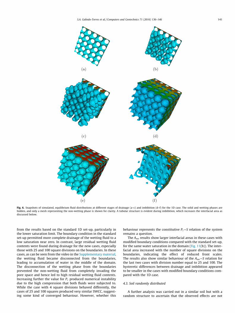
In the first case (called 1D hereafter), the simulation was basedon a 1D configuration with wetting and non-wetting fluid pres-sures set on two opposing boundaries respectively as shown inFig. 5(c). This is similar to the set-up of a pressure cell standarddevice used to measure the Pc—S curve (see Fig. 5(a)). This is awidely used design to measure the SWCC [13] where the boundaryconditions are the same as in the 1D case. Snapshots of thesimulated fluid distributions at different stages (Pc level) of thesimulation are shown in Fig. 6. Note that these are equilibriumresults. During drainage, the non-wetting fluid invaded the porousmedium with a pattern of tubular structures moving through thechannels (connected pore space) formed by the regular spherepacking. Clear separation between the wetting and non-wettingfluids across the cell was evident. During imbibition of the wettingphase, the separation of the two fluids at the cell scale becameeven more profound, with a relatively uniform, flat interfacialgeometry. A video of animated simulation results included in theSupplementary material shows these changes in sequence. Thestandard 1D set-up according to the pressure cell results in a sharpfront separating the wetting and non-wetting fluids across the sim-ulation domain/device, which is strongly linked with vertical fluidflows during the transient state in response to changes of the non-wetting fluid pressure on the top boundary.

The analysis led to the SWCC as shown in Fig. 7, where theprimary drainage and imbibition curves are fitted with the VanGenuchten (VG) function [14]. To show the bounds set by theprimary curves, several scanning curves (similar Pc—S drainageand imbibition curves but with smaller Pc ranges) obtained fromsimulations with different limit values of Pc are also plotted.Overall these simulated water retention curves are in qualitativeagreement with experimental observations, including the non-zero and non-unity limits of S, which reflect the trapped residualcontents of wetting and non-wetting fluid towards the end ofdrainage and imbibition, respectively (Fig. 6).

In the second case (called 3D hereafter), pressure boundary con-ditions are applied to the six faces of the cubic domain (Fig. 5(d)).These conditions replace the no flow boundary conditions onopposing four faces adopted in the first case. Three adjacent facescontrol the pressure for the wetting phase and the remaining threefaces control the pressure of the non-wetting phase. As shown inFig. 8, the change of the boundary conditions led to different fluiddistributions from those simulated in the 1D case at all stages ofthe drainage and imbibition cycles. The non-wetting fluid comingfrom the three controlling faces merged close to the corners, elim-inating the tubular structures during drainage (which was evidentin the 1D case). The flatter/smoother front in the 3D case wouldresult in a lower interfacial area Anw for the same saturation duringdrainage.

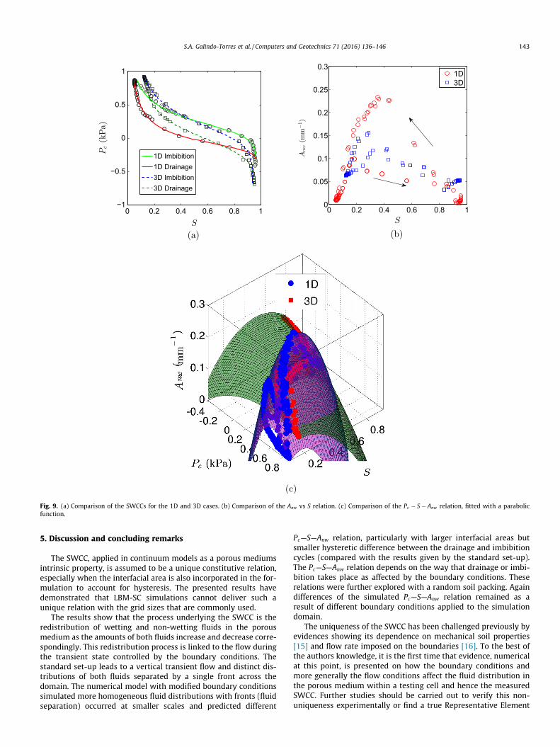
The SWCC curves were also determined for the 3D case simula-tion. The primary drainage and imbibition curves were found todiffer significantly from those for the 1D case (Fig. 9(a)). The 3Dcase exhibits a smaller hysteresis loop area. The lower limits ofthe wetting fluid saturation are also very different between thetwo cases, showing how the amount of the fluids trapped withinthe cycles depends on the boundary conditions. To further examinethe upscaling of the Pc—S relation, the interfacial area per void vol-ume (Anw in units of mm�1) between the wetting and non-wetting

(a) (b)

(c) (d)

Fig. 5. (a) Shows a typical pressure cell where water and air enter from opposite sides. (b) Shows the LBMmodel configuration for the standard pressure set-up with a regulararray of spheres representing the granular material. For the purpose of convenience, a cubic cell is simulated with a 1 cm side length and grains with a diameter of 2 mm. Theresults from the simulation show clearly the presence of a sharp front across the cell with the standard set-up. In the figure only the non-wetting phase is shown for the casewith the standard cell set-up. (c) and (d) Shows that different boundary conditions applied to a pressure cell produce different wetting fronts, even for the same saturation of50%, potentially leading to different SWCC.

140 S.A. Galindo-Torres et al. / Computers and Geotechnics 71 (2016) 136–146

fluids was also determined from the simulation results. Asdescribed previously, cells forming the interface between wettingand non-wetting fluids were identified and subsequently meshedwith a triangular tessellation to facilitate the calculation of theinterfacial area. Fig. 9(b) shows the measured area for the twocases with different boundary conditions. The tubular structureevident in the snapshots shown in Fig. 6 produced a large interfa-cial area during drainage in the 1D case while the more homoge-neous 3D condition presented a small variation in the interfacialarea between the two main cycles.

As discussed in the introduction, the multivariate Pc—S—Anw

relation has been assumed to represent the porous mediumsintrinsic property, taking a unique form with hysteresis incorpo-rated. This relation was also examined based on the simulationresults. The Pc—S—Anw data were fitted with a second orderbi-dimensional polynomial function for the 1D and 3D case,respectively. The fitting results were satisfactory with very highregression coefficients obtained for both cases (Fig. 9(c)). However,the fitted functions differed significantly between the two cases, asshown by the surfaces plotted in Fig. 9(c) and fitted coefficientvalues of the functions. No unique Pc—S—Anw relation could befound. Attempt was also made to fit all the data with a single

function; however, the result was far from satisfactory with a verylow regression coefficient value, indicating scatters in the data andnon-unique Pc—S—Anw relation between the cases.

4.2. Non uniform boundary conditions

To explore the effect of the front formed in the simulations forboth cases in relation to this non-unique Pc—S—Anw behaviour,we modified the boundary conditions to avoid net flows in anyparticular direction. The cube faces were divided equally into anumber of squares where alternating wetting and non-wettingfluid pressures were specified (Fig. 10(a)–(d)). Four cases were con-sidered with different numbers of square divisions. Both fluids,being equally injected into or pushed out of the cell from all sides,experienced zero net flow in all directions. As a result, the frontbecame fragmented with smaller length scales than the size ofthe domain. The system became increasingly more homogeneousacross the domain with the length scale of the front decreasingas the number of square divisions on the boundaries increased(Fig. 10(e)–(h)).

The SWCCs obtained from the simulations for the four addi-tional cases also showed different Pc—S behaviours (Fig. 11(a))

(a) (b)

(c) (d)

(e) (f)

Fig. 6. Snapshots of simulated, equilibrium fluid distributions at different stages of drainage (a–c) and imbibition (d–f) for the 1D case. The solid and wetting phases arehidden, and only a mesh representing the non-wetting phase is shown for clarity. A tubular structure is evident during imbibition, which increases the interfacial area asdiscussed below.

S.A. Galindo-Torres et al. / Computers and Geotechnics 71 (2016) 136–146 141

from the results based on the standard 1D set-up, particularly inthe lower saturation limit. The boundary condition in the standardset-up permitted more complete drainage of the wetting fluid to alow saturation near zero. In contrast, large residual wetting fluidcontents were found during drainage for the new cases, especiallythose with 25 and 100 square divisions on the boundaries. In thesecases, as can be seen from the video in the Supplementary material,the wetting fluid became disconnected from the boundaries,leading to accumulation of water in the middle of the domain.The disconnection of the wetting phase from the boundariesprevented the non-wetting fluid from completely invading thepore space and hence led to high residual wetting fluid contents.Increasing further the value for Pc produced numerical instabilitydue to the high compression that both fluids were subjected to.While the case with 4 square divisions behaved differently, thecases of 25 and 100 squares produced very similar SWCC, suggest-ing some kind of converged behaviour. However, whether this

behaviour represents the constitutive Pc—S relation of the systemremains a question.

The Anw results show larger interfacial areas in these cases withmodified boundary conditions compared with the standard set-up,for the same water saturation in the domain (Fig. 11(b)). The inter-facial area increased with the number of square divisions on theboundaries, indicating the effect of reduced front scales.The results also show similar behaviour of the Anw—S relation forthe last two cases with division number equal to 25 and 100. Thehysteretic differences between drainage and imbibition appearedto be smaller in the cases with modified boundary conditions com-pared with the 1D case.

4.3. Soil randomly distributed

A further analysis was carried out in a similar soil but with arandom structure to ascertain that the observed effects are not

0 0.2 0.4 0.6 0.8 1−0.5

0

0.5

1

Drainage

Imbibition

Fig. 7. SWCC for the 1D case showing the drainage and imbibition curves fittedwith the VG model. The different symbols show results from simulations ofdifferent scanning curves. The arrows indicate the progression of the drainage andimbibition cycle.

(a)

(c)

Fig. 8. Snapshots of simulated, equilibrium fluid distributions at different stages of drainare hidden, and only a mesh representing the non-wetting phase is shown for clarity.

142 S.A. Galindo-Torres et al. / Computers and Geotechnics 71 (2016) 136–146

due to the highly organized soil structure simulated. The porosityis slightly lower in the random soil (0.40 compared with 0.43 inthe regular soil). The same 1D and 3D boundary conditions areimposed over the domain. Fig. 12 shows different snapshots ofthe results for each boundary condition. These results show thatthe fluid is distributed in a more random way with more discon-nected pockets after each imbibition and drainage cycles. Thereis no longer a tubular structure like that shown in the previouscase, which explains the large difference in the interfacial areacompared with previous cases (for the regular soil).

Fig. 13 shows the different variables plotted for the 1D and 3Dcases. The Pc—S curves are now narrower for both cases but thedependence of the Pc—S relation on the boundary conditions areclearly evident in the simulations with the random soil. The limitvalues for Pc are smaller compared to the cases with the regularsoil. This indicates an increased capillary effect on the wetting ofthe porous medium due to its lower porosity and pore size, whichin turn reduces the value of Pc required to fully drain the med-ium. The dependence of the Pc—S—Anw relation on the boundaryconditions remains evident in the difference of the resultsbetween the 1D and 3D cases. The boundary effect seems to beless pronounced due to the absence of tubular structures duringthe imbibition of the non-wetting phase seen in the regular soilcases.

(b)

(d)

age (a and b) and imbibition (c and d) for the 3D case. The solid and wetting phases

0 0.2 0.4 0.6 0.8 1−1

−0.5

0

0.5

1

1D Imbibition1D Drainage3D Imbibition3D Drainage

(a)

0 0.2 0.4 0.6 0.8 10

0.05

0.1

0.15

0.2

0.25

0.31D3D

(b)

(c)

Fig. 9. (a) Comparison of the SWCCs for the 1D and 3D cases. (b) Comparison of the Anw vs S relation. (c) Comparison of the Pc � S� Anw relation, fitted with a parabolicfunction.

S.A. Galindo-Torres et al. / Computers and Geotechnics 71 (2016) 136–146 143

5. Discussion and concluding remarks

The SWCC, applied in continuum models as a porous mediumsintrinsic property, is assumed to be a unique constitutive relation,especially when the interfacial area is also incorporated in the for-mulation to account for hysteresis. The presented results havedemonstrated that LBM-SC simulations cannot deliver such aunique relation with the grid sizes that are commonly used.

The results show that the process underlying the SWCC is theredistribution of wetting and non-wetting fluids in the porousmedium as the amounts of both fluids increase and decrease corre-spondingly. This redistribution process is linked to the flow duringthe transient state controlled by the boundary conditions. Thestandard set-up leads to a vertical transient flow and distinct dis-tributions of both fluids separated by a single front across thedomain. The numerical model with modified boundary conditionssimulated more homogeneous fluid distributions with fronts (fluidseparation) occurred at smaller scales and predicted different

Pc—S—Anw relation, particularly with larger interfacial areas butsmaller hysteretic difference between the drainage and imbibitioncycles (compared with the results given by the standard set-up).The Pc—S—Anw relation depends on the way that drainage or imbi-bition takes place as affected by the boundary conditions. Theserelations were further explored with a random soil packing. Againdifferences of the simulated Pc—S—Anw relation remained as aresult of different boundary conditions applied to the simulationdomain.

The uniqueness of the SWCC has been challenged previously byevidences showing its dependence on mechanical soil properties[15] and flow rate imposed on the boundaries [16]. To the best ofthe authors knowledge, it is the first time that evidence, numericalat this point, is presented on how the boundary conditions andmore generally the flow conditions affect the fluid distribution inthe porous medium within a testing cell and hence the measuredSWCC. Further studies should be carried out to verify this non-uniqueness experimentally or find a true Representative Element

0 0.2 0.4 0.6 0.8 1−1

−0.5

0

0.5

1

1.5100 Squares25 Squares4 Squares1 Square1D Imbibition1D Drainage

(a)

0 0.2 0.4 0.6 0.8 10

0.05

0.1

0.15

0.2

0.25

0.3

0.35100 Squares25 Squares4 Squares1 Squares

(b)

Fig. 11. (a) SWCCs for the four cases with modified boundary conditions illustrated in Fig. 10. The main cycles are fitted with the VG function for the first two cases only. TheVG fitted for the 1D case of Fig. 7 is also shown for comparison. (b) Interfacial area Anw as a function of saturation. A line is drawn between consecutive points to help visualizethe point sequence.

(a) (b) (c) (d)

(e) (f) (g) (h)

Fig. 12. Snapshots of simulated, equilibrium fluid distributions at different stages of drainage and imbibition for both the 1D (a–d) and 3D (e–h) cases within the random soil.The solid and wetting phases are hidden, and only a mesh representing the non-wetting phase is shown for clarity.

(a) 1 square (b) 4 squares (c) 25 squares (d) 100 squares

(e) 1 square (f) 4 squares (g) 25 squares (h) 100 squares

Fig. 10. (a)–(d) Four different boundary conditions. The faces of the cube are divided in equal square areas with alternating injection of wetting and non-wetting fluids. In thelast three cases, the same number of injection squares are introduced for both phases. The only exception is the first case where 4 faces contain the non-wetting fluid with theremaining 2 injecting the wetting phase. (e)–(h) Different snapshots of the four cases showing how the fluid front becomes fragmented and how the fluid distributionstrongly depends on the boundary conditions.

144 S.A. Galindo-Torres et al. / Computers and Geotechnics 71 (2016) 136–146

0 0.2 0.4 0.6 0.8 1−0.2

−0.1

0

0.1

0.2

0.3

0.41D Imbibition1D Drainage3D Imbibition3D Drainage

(a)

0 0.2 0.4 0.6 0.8 11.25

1.3

1.35

1.4

1.45

1D3D

(b)

−0.10

0.10.2

0.3 0.20.4

0.60.8

0.5

1

1.5

1D

3D

(c)

Fig. 13. (a) Comparison of the SWCCs for the 1D and 3D cases in the random soil. (b) Comparison of the Anw vs S relation. (c) Comparison of the Pc � S� Anw relation, fittedwith a parabolic function.

S.A. Galindo-Torres et al. / Computers and Geotechnics 71 (2016) 136–146 145

Volume for the LBM simulations, which, as shown by this work,may be considerably larger than previously expected.

Acknowledgements

This work was funded by the ARC Discovery project(DP140100490) Qualitative and quantitative modelling of hydrau-lic fracturing of brittle materials. The first author also wants toacknowledge the support from the University of Queensland EarlyCareer Research Award (RM2011002323). The simulations werecarried out using the Mechsys open source library on the Macondohigh performance computing cluster of the University ofQueensland.

Appendix A. Supplementary data

Supplementary data associated with this article can be found, inthe online version, at http://dx.doi.org/10.1016/j.compgeo.2015.

09.008.These data include MOL files and InChiKeys of the mostimportant compounds described in this article.

References

[1] Shan X, Chen H. Lattice Boltzmann model for simulating flows with multiplephases and components. Phys Rev E 1993;47:1815–9. http://dx.doi.org/10.1103/PhysRevE.47.1815.

[2] Schaap M, Porter M, Christensen B, Wildenschild D. Comparison of pressure–saturation characteristics derived from computed tomography and latticeBoltzmann simulations. Water Resour Res 2007;43(12):W12S06.

[3] Porter ML, Schaap MG, Wildenschild D. Lattice-Boltzmann simulations of thecapillary pressure saturation interfacial area relationship for porous media.Adv Water Resour 2009;32(11):1632–40. http://dx.doi.org/10.1016/j.advwatres.2009.08.009. URL<http://www.sciencedirect.com/science/article/pii/S0309170809001328>.

[4] Hassanizadeh S, Gray WG. Mechanics and thermodynamics of multiphase flowin porous media including interphase boundaries. Adv Water Resour 1990;13(4):169–86. http://dx.doi.org/10.1016/0309-1708(90)90040-B. URL <http://www.sciencedirect.com/science/article/pii/030917089090040B>.

[5] Joekar-Niasar V, Hassanizadeh S, Leijnse A. Insights into the relationshipsamong capillary pressure, saturation, interfacial area and relative permeability

146 S.A. Galindo-Torres et al. / Computers and Geotechnics 71 (2016) 136–146

using pore-network modeling. Transp. Porous Media 2008;74(2):201–19.http://dx.doi.org/10.1007/s11242-007-9191-7. URL <http://dx.doi.org/10.1007/s11242-007-9191-7>.

[6] Culligan KA, Wildenschild D, Christensen BSB, Gray WG, Rivers ML, TompsonAFB. Interfacial area measurements for unsaturated flow through a porousmedium. Water Resour Res 2004;40(12):n/a–a. http://dx.doi.org/10.1029/2004WR003278. URL <http://dx.doi.org/10.1029/2004WR003278>.

[7] Galindo-Torres S. A coupled discrete element lattice Boltzmann method for thesimulation of fluid solid interaction with particles of general shapes. ComputMethods Appl Mech Eng 2013;265(0):107–19. http://dx.doi.org/10.1016/j.cma.2013.06.004.

[8] Sukop M, Thorne D. Lattice Boltzmann modeling: an introduction forgeoscientists and engineers. Springer Verlag; 2006.

[9] Qian Y, d’Humieres D, Lallemand P. Lattice BGK models for Navier–Stokesequation. EPL (Europhys Lett) 1992;17:479.

[10] He X, Luo L. Lattice Boltzmann model for the incompressible Navier–Stokesequation. J Stat Phys 1997;88(3):927–44.

[11] Martys NS, Chen H. Simulation of multicomponent fluids in complex three-dimensional geometries by the lattice Boltzmann method. Phys Rev E1996;53:743–50. http://dx.doi.org/10.1103/PhysRevE.53.743.

[12] Shan X, Doolen G. Multicomponent lattice-Boltzmannmodel with interparticleinteraction. J Stat Phys 1995;81(1):379–93.

[13] Drake SS, O’Carroll DM, Gerhard JI. Wettability contrasts between fresh andweathered diesel fuels. J Contam Hydrol 2013;144(1):46–57. http://dx.doi.org/10.1016/j.jconhyd.2012.09.008. URL <http://www.sciencedirect.com/science/article/pii/S0169772212001301>.

[14] Van Genuchten MT. A closed-form equation for predicting the hydraulicconductivity of unsaturated soils. Soil Sci Soc Am J 1980;44(5):892–8.

[15] Malaya C, Sreedeep S. Critical review on the parameters influencing soil–watercharacteristic curve. J Irrigat Drain Eng 2012;138(1):55–62. http://dx.doi.org/10.1061/(ASCE)IR.1943-4774.0000371.

[16] Wildenschild D, Hopmans J, Simunek J. Flow rate dependence of soil hydrauliccharacteristics. Soil Sci Soc Am J 2001;65(1):35–48.