Boundary Element and Finite Element Methods

MTH-ME82 Boundary Element and Finite Element Methods

Course details

20 Lectures

3 hour exam. Choose 3 out of 4 questions.

Recommended Text

Pozrikidis, C. (1992) Boundary Integral & Singularity Methods for Linearised Viscous Flow,

Cambridge.

There is one copy of this book in the library.

Problem sheet

One exercise sheet contains assorted problems covering the whole course. One question

from the exercise sheet will appear verbatim on the summer exam paper.

Contents

1. Background material.

2. Boundary integral methods for potential flow: Laplace’s equation, Poisson’s equation.

3. Boundary integral methods for Stokes flow

4. The Finite Element Method


1. Background

We will start by covering some background material, some of which you may already

be familiar with, to prepare for the main course material.

1.1 Index notation

In standard index notation, we represent the components of a vector using a subscript.

So

ui

for i = 1, . . . , 3 represents the three-dimensional vector u = (u1, u2, u3).

Definition: The Kronecker delta, δij , is defined by

δij =

0 if i 6= j

1 if i = j

So δ12 = 0 and δ22 = 1 and so on. If we write this as a matrix (assuming i = 1, 2 and

j = 1, 2) we have (1 0

0 1

),

we recognise it as the 2× 2 identity matrix.

Definition: The alternating tensor, εijk, is defined as

εijk =

0 if any of i, j, k are equal

1 if i, j, k are in cyclic order

−1 otherwise.

So, for example,

ε123 = ε231 = 1, ε132 = −1, ε133 = 0.

The alternating tensor provides a convenient way of expressing a vector (cross) product in

index notation.

Exercise: Show that εijkajbk is equal to the ith component of a × b by writing out the

components.

Einstein’s summation convention: According to this convention we sum over an index when-

ever we see it repeated (the range of the sum will be obvious from the context). For example,

for a calculation in three dimensions, i = 1, 2, 3, and

aii means3∑i=1

aii.

2


For a calculation in two dimensions, i = 1, 2, and

bii means2∑i=1

bii.

For example, δii = 2 in two dimensions, and δii = 3 in three dimensions.

Index shifting: The Kronecker delta is useful for shifting the index of a vector. For example,

we can write

ui = δij uj .

The summation convention is being used here to sum over the repeated index j on the right

hand side. Note that the only non-zero contribution to the sum comes when i = j, and

thus we recover the term on the left hand side.

1.2 The delta function

The delta function is an example of a generalised function or distribution. Informally,

we express the delta function as

δ(x) =

0 if x 6= 0

∞ if x = 0

We will not need the formal theory behind the delta function here1. However, we will make

use of the following property.

Sifting property: When a delta function multiplies another function inside an integral, the

result is the value of that function at the point where the argument of the delta function

vanishes. So, ∫ ∞−∞

δ(x)f(x) dx = f(0).

The delta function sifts out all values of f except that at x = 0. Also,∫ ∞−∞

δ(x− a)f(x) dx = f(a).

The delta function sifts out all values of f except that at x = a.

1.3 The principal value of an integral

Consider the following divergent (or improper) integral,∫ 1

−1

1

xdx.

1If you are interested, a good book is Applied Functional Analysis by D. Griffel.

3


There is evidently a problem with the integrand at x = 0. Proceeding carefully, we re-write

the integral as ∫ 1

−1

1

xdx = lim

ε→0

[ ∫ −ε−1

1

xdx+

∫ 1

ε

1

xdx].

Integrating, we have

limε→0

[ln |ε| − ln | − 1|+ ln |1| − ln |ε|

]= 0.

However, we could equally have re-written the integral as∫ 1

−1

1

xdx = lim

ε→0

[ ∫ −aε−1

1

xdx+

∫ 1

ε

1

xdx],

for any a > 0. Integrating, we find

limε→0

[ln |aε| − ln | − 1|+ ln |1| − ln |ε|

]= ln a,

and we can choose a to get any result we want!

Definition: The principal value of the integral∫ 1

−1

1

xdx

is defined to be

PV

∫ 1

−1

1

xdx = lim

ε→0

[ ∫ −ε−1

1

xdx+

∫ 1

ε

1

xdx]

= 0.

The principal value of other improper integrals is defined in a similar way.

1.4 Applications of the Boundary Integral Method

Potential Flow

A potential flow is one which is both inviscid and irrotational. Consider a steady (time-

independent) flow with velocity field u. If the flow is inviscid, then u satisfies the Euler

equations

(u · ∇)u = −∇p,

where p is the fluid pressure. The flow is irrotational if

∇× u = 0.

In this case we can define a scalar potential, φ, such that

u = ∇φ.

Conservation of mass requires that

∇ · u = 0.

4


Substituting u = ∇φ, we find

∇2φ = 0. (1.1)

So a potential flow satisfies Laplace’s equation.

For a potential flow, the boundary condition at a solid wall is

u · n = 0,

where n is the normal to the wall. This is called the normal flow condition and it demands

that fluid not pass through the solid wall. Since u = ∇φ, the condition may be written

∇φ · n = 0 or∂φ

∂n= 0, (1.2)

on the solid wall.

A typical potential flow problem might require us to solve (1.1) subject to (1.2). If the

geometry of the flow domain is simple, like a circle say, then this may be straightforward.

Example: Solve the equation

∇2φ = 0

in the circle 0 ≤ r ≤ 1 with φ = 1 on r = 1. In polar coordinates (assuming no θ

dependence), Laplace’s equation becomes

1

r

d

dr

(r

dφ

dr

)= 0.

Integrating, we find

φ = A log r +B.

We set A = 0 to remove the singularity at r = 0, and require B = 1 to satisfy the boundary

condition on the circle. So the solution is φ = 1.

Exercise: Think about how you would solve the same problem as above in a domain with

a more complex geometry. How would you satisfy the boundary condition φ = 1 on a

boundary with a complicated shape?

Electrostatics

A conducting metal sphere of given radius is charged to a potential φ = 1 and held above

flat ground at z = 0 where the potential is zero, φ = 0. The electric field outside the sphere

satisfies Laplace’s equation,

∇2φ = 0.

Compute the electric potential φ outside the sphere. This problem can be solved using the

Boundary Integral Method. Moreover, it can still be solved if the sphere is deformed to

some other shape.

5


Stokes flow

Stokes flow occurs at small values of the Reynolds number (we will discuss this more closely

later in the course). The Boundary Integral Method has been applied to a host of different

problems in Stokes flow. Examples include:

• Oscillations of a gas bubble

• Bursting of a bubble near to a wall or a free surface

• Flow of a viscous fluid film over a shaped surface

• Deformation of red blood cells passing through capillaries

• Break-up of a viscous liquid jet

2. The boundary integral method (BIM) for potential flow

Over the last 30 or so years, a very popular method for solving Stokes flows in intricate

geometries has developed and matured. This nifty method calculates a Stokes flow solely by

reference to what happens at the flow boundaries. As we will see, we can write the velocity

at any point in the flow field purely in terms of the flow quantites on the boundaries. The

method is called the boundary integral method.

The historical development of the mathematical machinery sitting behind the boundary

integral method is nicely reviewed in the paper Cheng & Cheng (2005) Heritage and early

history of the boundary element method, Eng. Analysis Bound. Elem., 29, 268-302.

The main advantage of the boundary integral method for solving certain classes of PDEs is

as follows: Since reference is only made to boundary values, the dimension of the problem

is effectively reduced by one. So a three dimensional problem effectively becomes a two

dimensional problem. This brings about a tremendous saving in computing time.

Its is an extremely powerful method for this reason: It can cope with any geometry at

all. Since many practical applications involve very complex geometries, this constitutes a

major advantage over other methods such as finite differences which are very clumsy if the

geometry is not simple.

The boundary integral method can be applied to both potential flows and Stokes flows.

Since the implementation of the former is slightly easier, it is these which we shall discuss

first.

2.1 The BIM for potential flow in two dimensions

Aim: To solve Laplace’s equation inside a domain D, with boundary C whose unit normal

n is defined to point inside D.

6


We take as our starting point Green’s second identity,

ψ∇2φ− φ∇2ψ = ∇ · (ψ∇φ− φ∇ψ). (2.1)

We choose ψ = G, where G satisfies the equation

∇2G+ δ(x− x0) = 0, (2.2)

where the second term is the delta function.

Definition: We call x0 the pole or the singular point or just the singularity.

nb: G is called a fundamental solution of Laplace’s equation or Green’s function2 (we will

discuss these in more detail later).

Let us define

r = |x− x0|,

so that r is the distance from x0 to x. When r 6= 0 (2.2) becomes

∇2G = 0, (2.3)

or (assuming G only depends on r)

1

r

d

dr

(r

dG

dr

)= 0.

We notice that

G = λ log r, (2.4)

for constant λ, is a solution. For reasons to be revealed, we choose λ = −1/2π.

Definition: The fundamental solution to Laplace’s equation,

G = − 1

2πlog r, (2.5)

is called the free-space Green’s function.

In the next step, we integrate (2.1) over the domain D. In fact, to avoid the problem with

the delta function at x = x0, we delete from D a small disk, Dε, of radius ε centred at x0.

Then we define D′ = D −Dε and integrate (2.1) over D′:∫∫D′

(G∇2φ− φ∇2G) dS =

∫∫D′∇ · (G∇φ− φ∇G) dS = 0,

since both ∇2G = 0 and ∇2φ = 0 within D′. Using the divergence theorem we obtain∫C+Cε

(G∇φ− φ∇G) · n dl = 0, (2.6)

2Strictly speaking one should only refer to this as a Green’s function when it satisfies a boundary value

problem, that is G adopts prescribed values on a given boundary

7


where C is the boundary to D and Cε is the boundary to Dε, and l measures arc length

along either C or Cε.

Consider now the integral around Cε,

Iε =

∫Cε

(G∇φ− φ∇G) · n dl

In the limit ε→ 0, the radius of the disk shrinks to zero. From (2.4)

G = λ log r.

Therefore

Iε =

∫Cε

(λ log r

∂φ

∂r− λφ

r

)dl.

Since r = ε on Cε, letting ε→ 0, we find

Iε = λ(log ε)∂φ

∂r(x0)

∫Cε

dl−λφ(x0)

ε

∫Cε

dl = 2πλ(ε log ε)∂φ

∂r(x0)−2πλε

φ(x0)

ε= −2πλφ(x0).

Rearranging (2.6) we have ∫C

(G∇2φ− φ∇2G) dS = 2πλφ(x0),

and so

φ(x0) = − 1

2πλ

∫C

(φ∇2G−G∇2φ) dS. (2.7)

For tidiness, we choose λ = −1/2π. Substituting for G we have

φ(x0) =1

2π

[ ∫C

log r n · ∇φ dl −∫Cφ n · ∇ log r dl

]. (2.8)

This is called Green’s third identity. In fact equation (2.7) applies for a general Green’s

function G which satisfies (2.2) and any chosen boundary conditions.

Definition: The boundary integral equation (BIE) for potential flow is given by

φ(x0) =

∫Cφ n · ∇G−G n · ∇φ dl, (2.9)

where the unit normal to the boundary C, n, points inside the solution domain D.

Note : Equation (2.8) is an example of an integral equation. Although φ appears as the

subject on the left hand side, the function φ and its derivatives also appear on the right

hand side inside the integrals.

Other Green’s functions

8


It is worth emphasizing at this stage that a Green’s function is simply a device to enable us

to solve problems. In the present scenario, we will use a Green’s function to help us solve

Laplace’s equation

∇2φ = 0

subject to some boundary condition, for example

φ = 0 on Γ,

where Γ represents a boundary. The solution which we end up with does not depend on the

Green’s function used to obtain it. In this sense, we can think of a Green’s function simply

as a tool which is used to create an end product; but the end product itself is not changed

by the particular choice of tool used to put it together.

Above we derived the free space Green’s function,

G = − 1

2πlog r,

where r = |x − x0| and x0 is the location of the singularity. In some cases, it is expedient

to select a Green’s function which vanishes (or its derivative vanishes) on the boundary. A

simple example is a Green’s function for a singularity x0 = (x0, y0) (with y0 > 0) placed

above a plane wall at y = 0. The Green’s function is required to vanish at the wall, that is

G = 0 when y = 0.

We can construct this Green’s function by placing an image singularity of opposite

sign3 below the wall at y = −y0. We write down the free-space Green’s function for each

singularity and add them together, thus

G = − 1

2πlog r +

1

2πlogR,

where

r =√

(x− x0)2 + (y − y0)2, R =√

(x− x0)2 + (y + y0)2.

So

G = − 1

4πlog

(x− x0)2 + (y + y0)2

(x− x0)2 + (y − y0)2

Now, setting y = 0 we obtain

G = − 1

4πlog

(x− x0)2 + y2

0

(x− x0)2 + y20

= 0,

as required.

Alternatively, we may instead wish to construct a Green’s function whose y-derivative

vanishes at the wall. After come experimenting, we notice that

G = − 1

2πlog r − 1

2πlogR,

3By this we mean that we take G = (1/2π) log r rather than G = −(1/2π) log r

9


fits the bill. To check, we differentiate with respect to y to obtain

Gy = − 1

2π

ryr− 1

2π

RyR.

Now,

ry =y − y0

r, ry =

y + y0

R.

So,

Gy = − 1

2π

y − y0

r2− 1

2π

y + y0

R2.

Setting y = 0 we find

Gy =1

2π

y0

r2− 1

2π

y0

R2= 0,

as required.

Periodic Green’s functions

Sometimes it is useful to work with a periodic Green’s function which satisfies a periodic

relation, for example

G(x, y;x0, y0) = G(x+ L, y;x0, y0),

for some L > 0. One example is a periodic array of singularities located at the positions

(x0 ± nL, y0)

for n = 0, 1, 2, . . .. After some working we find

G = − 1

4πlog

2cosh(k[y − y0])− cos(k[x− x0]),

where k = 2π/L.

For a periodic array of singularities located above a wall at y = 0, with G required to vanish

at the wall, we have

G = − 1

4πlog

2cosh(k[y−y0])−cos(k[x−x0])

+1

4πlog

2cosh(k[y+y0])−cos(k[x−x0]).

Exercise: Check that the periodic Green’s function above has the property G = 0 when

y = 0. How would you modify the formula so that Gy = 0 on y = 0?

The Boundary Integral Method

Our goal is to solve (2.9) for φ. To make this more explicit, we write out (2.9) again showing

explicitly all the dependencies:

φ(x0) =

∫Cφ n(x) · ∇G(x,x0)−G(x,x0) n(x) · ∇φ(x) dl(x).

Note that

10


• x0 is the singular point in the interior of the domain D.

• x is the so-called field point.

• Integration is done with respect to arclength around C. Note that the local increment

of arc length, dl depends on x.

We notice that on the right hand side, the unknown function φ appears inside integrals

which are defined over the boundary C. So the right hand side is only concerned with

boundary values of φ. This suggests the following way to proceed:

(i) Take the point x0 to lie on the boundary C. Then the integral equation involves only

values of φ on the boundary.

(ii) Solve the integral equation for the boundary values of φ.

(iii) Once the boundary values of φ are known we can compute the right hand side of (2.8)

for any x0 inside D. Hence we can find φ everywhere in the domain D.

Points (i-iii) form the basic steps of the boundary integral method.

Step (i) requires us to take the point x0 to lie on C. This requires some careful thought.

Let’s work with a general Green’s function, G, and write out the boundary integral equation

(2.9)

φ(x0) =

∫Cφ(x) n · ∇G(x,x0) dl(x)−

∫CG(x,x0) n · ∇φ(x) dl(x). (2.10)

nb: We’ve written out explicitly the arguments on each function in (2.10) to keep clear the

functional dependencies.

On the right hand side of (2.10), there are two integrals,∫CG(x,x0) n · ∇φ(x) dl(x) and

∫Cφ(x) n · ∇G(x,x0) dl(x).

We call the first integral the single layer potential (SLP).

We call the second integral the double layer potential (DLP).

The limit x0 → C

It can be shown that the SLP is continuous as the point x0 approaches and then crosses C.

In contrast, as x0 crosses C, the double-layer potential undergoes a jump discontinuity. As

x0 approaches C from inside the domain D, we find (see the Problem Sheet)

limx0→C

∫Cφ(x) [n · ∇G(x,x0)] dl(x) =

∫ PV

Cφ(x)[n · ∇G(x,x0)] dl(x) +

1

2φ(x0), (2.11)

11


and when x0 approaches C from outside D, we find

limx0→C

∫Cφ(x) [n · ∇G(x,x0)] dl(x) =

∫ PV

Cφ(x)[n · ∇G(x,x0)] dl(x)− 1

2φ(x0). (2.12)

Note that on the right hand side of these equations x0 is located on C. (For multiply-

connected domains, inside is taken to mean the area into which the normal vector points.)

The superscript PV means that we are taking the principal value of the integral.

Example

Suppose that the domain D occupies the strip −1 ≤ x ≤ 1, y > 0, and label as L that part

of C lying on y = 0. Consider what happens to the DLP as x0 travels down the y axis

through L.

We have that x0 = (0, y0) as we are interested in what happens as y0 passes down

through zero from above. The unit normal on L pointing into D is the unit vector in the

positive y direction. So we have

n · ∇G =∂G

∂y.

Taking the free space Green’s function we have

∂G

∂y= − 1

2π

∂

∂y(log r) = − 1

2π

(y − y0)

r2.

since r2 = x2 + (y − y0)2 and∂r

∂y=

(y − y0)

r2.

So the DLP over L is

D =

∫Lφ(x) n · ∇G dx =

∫ 1

−1φ(x)

∂G

∂y

∣∣∣y=0

dx =1

2π

∫ 1

−1

φ(x) y0

x2 + y20

dx.

A difficulty will arise in the integral at x = 0 when y0 = 0. We rewrite as

D =1

2πy0

∫ 1

−1

φ(x)− φ(0)

x2 + y20

dx+1

2πφ(0)

∫ 1

−1

y0

x2 + y20

dx,

Consider the first integral. For small x, φ(x) = φ(0) + xφ′(0) + · · · . Hence near to x = 0,

limy0→0+

[φ(x)− φ(0)

x2 + y20

]≈ lim

y0→0+

[φ′(0)

x

x2 + y20

]= φ′(0)

1

x.

Therefore in the limit y0 → 0+ the first integral is improper and behaves like the integral∫ 1

−1

1

xdx.

To make sense of it in this limit, we take the principal value of the original integral. Therefore

we write, for y0 → 0+,

D =1

2πy0 PV

∫ 1

−1

φ(x)− φ(0)

x2 + y20

dx+1

2πφ(0) PV

∫ 1

−1

y0

x2 + y20

dx,

12


For the second integral, ∫ 1

−1

y0

x2 + y20

dx = 2 tan−1

(1

y0

).

We can see that the value of this integral is discontinuous at y0 = 0 since

limy0→0+

∫ 1

−1

y0

x2 + y20

dx = π, limy0→0−

∫ 1

−1

y0

x2 + y20

dx = −π.

When y0 is on L (so that y0 = 0) the integrand vanishes so that

PV

∫ 1

−1

y0

x2 + y20

dx = 0.

Putting everything together, then, we have that in the limit y0 → 0+,

D =1

2πy0 PV

∫ 1

−1

φ(x)− φ(0)

x2 + y20

dx+1

2πφ(0) PV

∫ 1

−1

y0

x2 + y20

dx+1

2ππφ(0),

and so

D =1

2πPV

∫ 1

−1

y0φ(x)

x2 + y20

dx+1

2φ(0).

Or, in the original form

D =

∫ PV

Lφ(x) n · ∇G dx+

1

2φ(0).

We can work along similar lines to show that as y0 approaches L from outside D, that is as

y0 → 0−,

D =

∫ PV

Lφ(x) n · ∇G dx− 1

2φ(0).

To complete step (i) of the boundary integral method, we let the point x0 approach C from

the inside in (2.10) and then, using (2.11), we obtain

φ(x0) =

∫ PV

Cφ(x) [n · ∇G(x,x0)] dl(x) +

1

2φ(x0)−

∫CG(x,x0) n · ∇φ(x) dl(x),

where x0 lies on C. So,

1

2φ(x0) =

∫ PV

Cφ(x) [n · ∇G(x,x0)] dl(x)−

∫CG(x,x0) n · ∇φ(x) dl(x),

where the unit normal to the boundary C, n, points inside the solution domain D. We now

introduce the flux q, which is defined4 so that q ≡ n · ∇φ. Then we have

1

2φ(x0) =

∫ PV

Cφ(x) [n · ∇G(x,x0)] dl(x)−

∫CG(x,x0) q(x) dl(x), (2.13)

4Why do we call this the flux? Fick’s law states that a substance flows down its concentration gradient

(like heat, for example). If φ represents the concentration of some substance, then −∇φ is its flow rate

according to Fick’s law. Then the flux out of a closed region with inward pointing normal n will be n · ∇φ.

13


where x0 lies on C.

If φ is prescribed on the boundary, then we have a Fredholm integral equation of the first

kind for the flux q, ∫CG(x,x0) q(x) dl(x) = F (x0),

where

F (x0) =

∫ PV

Cφ(x) [n · ∇G(x,x0)] dl(x)− 1

2φ(x0).

It is called an integral equation of the first kind since the subject (in this case q) appears

inside the integral but not on the right hand side.

If instead q is prescribed on the boundary C, we have a Fredholm integral equation of the

second kind for the boundary distribution of φ,

1

2φ(x0) =

∫ PV

Cφ(x) [n · ∇G(x,x0)] dl(x) + Φ(x0),

where

Φ(x0) = −∫CG(x,x0) q(x) dl(x).

It is called an integral equation of the second kind because the subject (in this case φ)

appears both inside the integral and outside of it.

Example problem 2.1

The function φ satisifes Laplace’s equation in the domain D inside the circle C of radius a,

∇2φ = 0,

with the boundary condition φ = 1 on C. Formulate the solution for φ using the BIM.

First let us note that the exact solution, which is regular everywhere inside the circle,

is φ = 1. Now, we start with the BIE for a point x0 lying on C, namely (2.13),

1

2φ(x0) =

∫ PV

Cφ n · ∇G−G q dl.

where q = n · ∇φ and noting that φ = 1 on C we have

1

2=

∫ PV

Cn · ∇G−G q dl.

We will use polar coordinates (ρ, θ) with origin at the centre of the circle. The unit normal

points into D in the negative radial direction, and so

1

2= PV

∫ 2π

0

(−∂G∂ρ

)ρ=a

a dθ − a∫ 2π

0G q dθ.

14


We will utilise the free space Green’s function, G = −(1/2π) log r, where r = [(x − x0)2 +

(y − y0)2]. It will be useful to note that when both (x, y) and (x0, y0) lie on C, using the

cosine rule we have

r2 = 2a2(1− cos θ), (2.14)

where θ is the angle subtended between the points (x, y) and (x0, y0) and the origin. Also,

when (x0, y0) lies at a general point in space,

r2 = a2 + ρ2 − 2aρ cos θ,

where again θ is the angle subtended between the points (x, y) and (x0, y0) and the origin.

Hence∂G

∂ρ=∂G

∂r

∂r

∂ρ= − 1

2πr

ρ− a cos θ

r= − 1

2π

ρ− a cos θ

r2.

So on ρ = a,

−∂G∂ρ

=a

2π

1− cos θ

r2=

1

4πa.

Therefore the BIE becomes1

2=

1

2+

a

2π

∫ 2π

0q log r dθ

and so ∫ 2π

0q log r dθ = 0. (2.15)

This is satisfied if we take q = 0 on ρ = a. According to the exact solution, φ = 1, we have

q(ρ = a) = n · ∇φ∣∣∣ρ=a

= φρ

∣∣∣ρ=a

= 0,

and so the two solutions are consistent.

Cautionary warning: When we reformulate a partial differential equation, such as

Laplace’s equation, as an integral equation, as we are doing here, we introduce the pos-

sibility of spurious solutions which satisfy the integral equation but not the original PDE.

To illustrate this, let us revisit the example above. We start by noting that when both x

and x0 are on C, using (2.14),∫ 2π

0log r dθ =

1

2

∫ 2π

0log[2a2(1− cos θ)] dθ = π log(2a2) +

1

2

∫ 2π

0log(1− cos θ) dθ.

Exercise: Show that ∫ 2π

0log(1− cos θ) dθ = −2π log 2.

So ∫ 2π

0log r dθ = 2π log a.

15


For the example problem, we derived the constraint on the boundary flux (2.15),∫ 2π

0q log r dθ = 0.

Consider what happens if we take the circle to be of unit radius, so that a = 1. Then we

have that ∫ 2π

0log r dθ = 0,

and so we may choose q = κ, where κ is any constant, to satisfy (2.15). But we know from

the exact solution that the only admissible value is κ = 0. This serves as a warning to be

on our guard when dealing with the integral formulation of a PDE.

2.2 The BIM for potential flow at a corner

The arguments in the previous section relied on the use of the divergence theorem,

which is applicable provided that the boundary C is piecewise smooth5. However, there

is a difficulty with allowing the point x0 to approach a point on a curve, such as a sharp

corner, where the normal vector is not continuous. In this case, the argument needs some

modification.

In practice, we are often interested in computing solutions in domains which involve corners

or kinks, for example a rectangular domain. In this section, we address how to adapt the

boundary integral method for potential flow to such regions.

To proceed, we go back to the beginning of the argument: Green’s second identity. This

states that

ψ∇2φ− φ∇2ψ = ∇ · (ψ∇φ− φ∇ψ).

Integrating over the domain, D, we obtain∫∫Dψ∇2φ− φ∇2ψ dS =

∫∫D∇ · (ψ∇φ− φ∇ψ) dS =

∫C

(ψ n · ∇φ− φ n · ∇ψ) dl

by the divergence theorem, which we note is still valid for a boundary with a corner.

As before, φ satisfies Laplace’s equation, ∇2φ = 0. For the sake of argument, we take ψ to

be the free-space Green’s function,

ψ = G = − 1

2πlog r,

satisfying

∇2G+ δ(x− x0) = 0.

5A curve is smooth if its normal vector is a continuous function of position. Such a curve or surface is

also called Lyapunov. A curve is piecewise smooth if its normal vector is continuous at finitely many points.

One such example is a square (e.g., Kreysig §10.5).

16


So,

−∫∫

Dφ∇2G dS =

∫C

(G n · ∇φ− φ n · ∇G) dl.

Consider now a point x0 which lies outside of the domain D. It follows that ∇2G = 0

leaving

0 =1

2π

∫C

(G n · ∇φ− φ n · ∇G) dl.

Substituting for G,

0 =1

2π

∫C

(log r n · ∇φ− φ n · ∇ log r) dl.

Since r = |x− x0|,

∇ log r =( ∂∂x,∂

∂y

)log r =

(x− x0

r2,y − y0

r2

)=

x− x0

r2.

Thus,

0 =1

2π

∫C

(log r n · ∇φ− φ n · x− x0

r2) dl (2.16)

(a) (b)

α

n

x0

ε

n

θ

x0

n

Figure 1: A domain with a sharp corner of angle α.

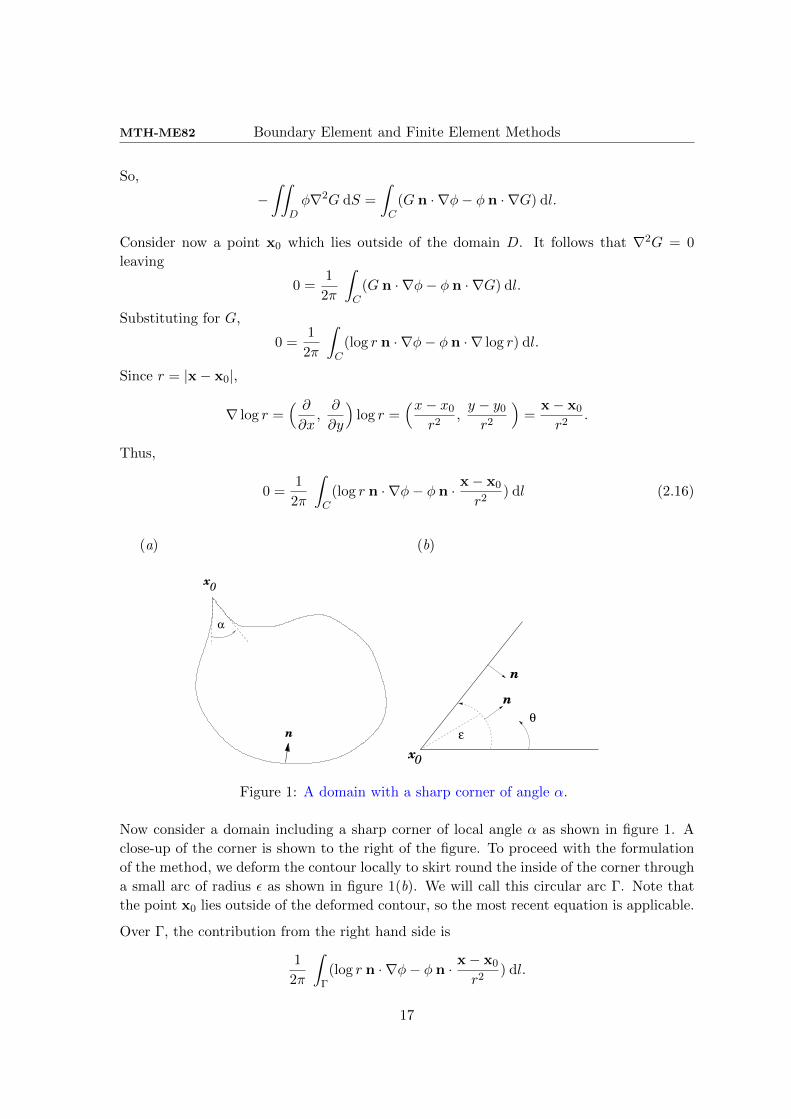
Now consider a domain including a sharp corner of local angle α as shown in figure 1. A

close-up of the corner is shown to the right of the figure. To proceed with the formulation

of the method, we deform the contour locally to skirt round the inside of the corner through

a small arc of radius ε as shown in figure 1(b). We will call this circular arc Γ. Note that

the point x0 lies outside of the deformed contour, so the most recent equation is applicable.

Over Γ, the contribution from the right hand side is

1

2π

∫Γ(log r n · ∇φ− φ n · x− x0

r2) dl.

17


On the arc, r = ε, x − x0 = ε cos θ and y − y0 = ε sin θ, where θ is the angle shown, and

dl = ε dθ giving,1

2πε

∫ α

0(log ε n · ∇φ− φ n · x− x0

ε2) dθ.

The unit normal to the arc

n =x− x0

r,

leaving

1

2πε

∫ α

0(log ε n · ∇φ− φ |x− x0|2

ε3) dθ =

1

2πε

∫ α

0(log ε n · ∇φ− φ

ε) dθ.

Also,

n · ∇φ =x− x0

r· ∇φ =

x− x0

r

∂φ

∂x+y − y0

r

∂φ

∂y,

giving1

2πε

∫ α

0

[log ε

(cos θ

∂φ

∂x+ sin θ

∂φ

∂y

)− φ

ε

]dθ

(since x− x0 = ε cos θ and y − y0 = ε sin θ)

=1

2π

∫ α

0

[ε log ε

(cos θ

∂φ

∂x+ sin θ

∂φ

∂y

)− φ

]dθ.

Now we let the arc Γ shrink to the corner point by taking the limit ε→ 0, i.e. we consider

limε→0

1

2π

∫ α

0

[ε log ε

(cos θ

∂φ

∂x+ sin θ

∂φ

∂y

)− φ

]dθ

Note that limε→0 ε log ε = 0. So,

limε→0

1

2π

∫ α

0

[ε log ε

(x− x0

r

∂φ

∂x+y − y0

r

∂φ

∂y

)− φ(x)

]dθ = − 1

2πφ(x0)

∫ α

0dθ = − α

2πφ(x0).

In summary,1

2π

∫Γ(log r n · ∇φ− φ n · x− x0

r2) dl = − α

2πφ(x0).

So,1

2π

∫C

(log r n · ∇φ− φ n · x− x0

r2) dl

=1

2πPV

∫C

(log r n · ∇φ− φ n · x− x0

r2) dl + lim

ε→0

1

2π

∫Γ(log r n · ∇φ− φ n · x− x0

r2) dl,

where the principal value PV refers to the fact that the small arc of radius ε has been

excluded from the integration.

Thus, (2.16) becomes1

2π

∫C

(log r n · ∇φ− φ n · x− x0

r2) dl

18


=1

2πPV

∫C

(log r n · ∇φ− φ n · x− x0

r2) dl − α

2πφ(x0) = 0.

Rearranging,α

2πφ(x0) =

1

2πPV

∫C

(log r n · ∇φ− φ n · x− x0

r2) dl

The previous equation was derived working with the free-space Green’s function. But it is

equally applicable to any Green’s function. So we may write in general,

α

2πφ(x0) = −

∫CG(x,x0) n · ∇φ(x) dl(x) +

∫ PV

Cφ(x) n · ∇G(x,x0) dl(x).

Note that the PV is only required on the 2nd integral as the first is continuous as x0

approaches the contour.

nb: If α = π, then there is no corner, and we recover our original boundary integral equation

(2.13),

1

2φ(x0) = −

∫CG(x,x0) n · ∇φ(x) dl(x) +

∫ PV

Cφ(x) n · ∇G(x,x0) dl(x).

Summary: Potential Flow

In this section we have:

• starting from Green’s second identity, derived the boundary integral equation (BIE)

for potential flow valid for a point x0 inside the domain of interest.

• introduced the notion of a Green’s function

• using the notion of a principal value, obtained the form of the BIE valid for a point

x0 lying on the contour enclosing the domain of interest.

• derived the form of the BIE valid for a contour with a sharp kink

3. The boundary element method (BEM) for potential flow

We have now established how to reformulate a partial differential equation as an integral

equation, and we have seen that the advantage in doing this is that the new formulation is

defined over a boundary of any shape. In contrast, traditional methods of solving PDEs,

for example separation of variables, usually require the boundary geometry to be relatively

simple.

Aim: The aim of this section is to see how to go about solving an integral equation for

potential flow numerically. The procedure is known as the Boundary Element Method

(BEM).

19


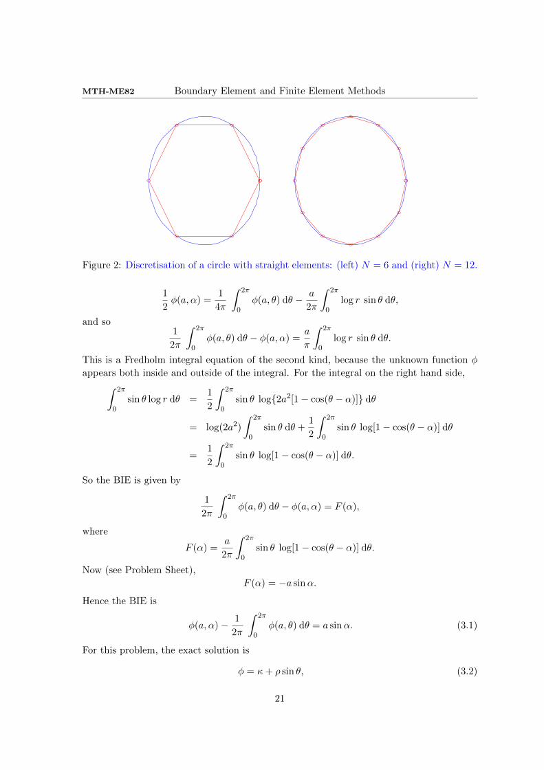
We demonstrate the method by way of a specific example. In short, the idea is to discretise

the boundary C of the solution domain D using a sequence of straight or curved boundary

elements over each of which the solution is approximated using constants or polynomial

approximations.

Example problem 3.1

Consider the inviscid, irrotational motion of fluid through a circle C of radius a. Inside the

circular domain, D, the velocity potential, φ, satisfies Laplace’s equation ∇2φ = 0. Fixing

polar coordinates (ρ, θ) with origin at the centre of the circle, fluid flows into and out of D

such that the normal component of velocity on C is given by

−n · ∇φ =∂φ

∂ρ

∣∣∣ρ=a

= sin θ,

where n = −eρ, where eρ is the unit vector pointing in the positive ρ direction, points into

D. Thus fluid flows out of D through ρ = a, 0 ≤ θ ≤ π, and fluid flows into D through

ρ = a, π ≤ θ ≤ 2π.

We reformulate the problem as an integral equation. Taking the BIE with the point,

x0, placed on C, we make use of equation (2.13), namely

1

2φ(x0) =

∫ PV

Cφ(x) [n · ∇G(x,x0)] dl(x)−

∫CG(x,x0) q(x) dl(x).

We will use the free space Green’s function,

G = − 1

2πlog r,

where r = |x−x0|. Using the information given in the question, we have q = n·∇φ = − sin θ,

and so the BIE becomes

1

2φ(a, α) = a PV

∫ 2π

0φ(a, θ)

(−∂G∂ρ

)ρ=a

dθ − a

2π

∫ 2π

0log r sin θ dθ.

Here θ is the angle subtended between x, x0 and the origin, and θ = α is the location of

the point x0 on the circle C. Using the cosine rule we know that

r2 = a2 + ρ2 − 2aρ cos(θ − α), r2 = 2a2[1− cos(θ − α)],

when ρ takes a general value and ρ = a respectively. Also

∂G

∂ρ=∂G

∂r

∂r

∂ρ= − 1

2πr

ρ− a cos(θ − α)

r= − 1

2π

ρ− a cos(θ − α)

r2.

and so (−∂G∂ρ

)ρ=a

=a

2π

1− cos(θ − α)

r2=

1

4πa.

So we have

20


Figure 2: Discretisation of a circle with straight elements: (left) N = 6 and (right) N = 12.

1

2φ(a, α) =

1

4π

∫ 2π

0φ(a, θ) dθ − a

2π

∫ 2π

0log r sin θ dθ,

and so1

2π

∫ 2π

0φ(a, θ) dθ − φ(a, α) =

a

π

∫ 2π

0log r sin θ dθ.

This is a Fredholm integral equation of the second kind, because the unknown function φ

appears both inside and outside of the integral. For the integral on the right hand side,∫ 2π

0sin θ log r dθ =

1

2

∫ 2π

0sin θ log2a2[1− cos(θ − α)] dθ

= log(2a2)

∫ 2π

0sin θ dθ +

1

2

∫ 2π

0sin θ log[1− cos(θ − α)] dθ

=1

2

∫ 2π

0sin θ log[1− cos(θ − α)] dθ.

So the BIE is given by

1

2π

∫ 2π

0φ(a, θ) dθ − φ(a, α) = F (α),

where

F (α) =a

2π

∫ 2π

0sin θ log[1− cos(θ − α)] dθ.

Now (see Problem Sheet),

F (α) = −a sinα.

Hence the BIE is

φ(a, α)− 1

2π

∫ 2π

0φ(a, θ) dθ = a sinα. (3.1)

For this problem, the exact solution is

φ = κ+ ρ sin θ, (3.2)

21


for any constant κ. Substituting this into the BIE, we confirm that it satisfies the equation.

Note in particular that we can add an arbitrary constant to φ in (3.1) without altering the

equation. We will return to this point below.

Assuming that we don’t know the exact solution, we proceed by discretising the bound-

ary with a sequence of boundary elements. We will use straight elements, and approximate

the circle with a regular polygon with N sides, with each vertex of the polygon lying on

C. Next we approximate the value of φ along the ith side/element with a constant φi,

for i = 1 . . . N . Then if θi is the angle subtended by the ith element and the origin, we

approximate the BIE (3.1) by replacing it with

φ(a, α)− 1

2π

N∑i=1

∫ θi+1

θi

φi dθ = a sinα,

where θN+1 = θ1. Notice that we have approximated the integral with a sum over the N

elements. Since we’re assuming that the φi are constant, we have

φ(a, α)− 1

2π

N∑i=1

φi

∫ θi+1

θi

dθ = a sinα,

and so

φ(a, α)− 1

2π

N∑i=1

φi di = a sinα, (3.3)

where

di = θi+1 − θi.

Next we apply (3.3) at the mid-point of each element to obtain the N equations

φj −1

2π

N∑i=1

φi di = a sinαj , (3.4)

for j = 1, . . . , N , where

αj =1

2(θj + θj+1),

and φj = φ(a, αj). We may write the system of N equations in (3.4) as a matrix system

A · x = b, (3.5)

where

x = (φ1, φ2, . . . , φN )T , b = a (sinα1, sinα2, . . . , sinαN )T ,

and A is a N ×N matrix which has the appropriate structure.

Problem: We noted above that the integral equation (3.1) is unchanged by adding a

constant to φ and so it has an infinite number of solutions. We should expect the linear

system (3.5) to have the same property, that is for the matrix A to be singular.

22


0 1 2 3 4 5 6−2.5

−2

−1.5

−1

−0.5

0

0.5

1

1.5

θ

φ(a

,θ)

BEM solution with N=16 straight elements

BEM

Exact

Figure 3: BEM solution to integral equation (3.3) with N = 16 elements and a = 2.0.

To get around the problem that detA = 0 and to obtain a solution to the problem, we will

fix the value of φ to be zero at the mid-point of the first element (this is tantamount to

fixing the constant κ in the exact solution 3.2), and solve the algebraic equations (3.4) for

j = 2, . . . , N . So now we have the adjusted linear system:

φ1 = 0, A · x = b, (3.6)

where

x = (φ2, . . . , φN )T , b = a (sinα2, . . . , sinαN )T ,

where A is a (N − 1) × (N − 1) matrix which has the appropriate structure (see Matlab

code BEMexample1.m).

We solve the linear system in (3.6) for x, using Gaussian elimination for example,

to determine the values of φ on the elements. This gives us an approximation to the

solution. As we increase N and take polygons with more and more sides, we more closely

approximate the circular boundary, and more closely approximate the true solution on the

boundary, φ = a sin θ. The result of an example calculation carried out using the Matlab

code BEMexample1.m with N = 16 elements for a = 2.0 is shown in figure 3.

3.1 The BEM for Poisson’s equation

Here we briefly discuss methods to solve Poisson’s equation, namely

∇2φ = −s(x), (3.7)

23


using the boundary element method.

Starting from Green’s second identity,

ψ∇2φ− φ∇2ψ = ∇ · (ψ∇φ− φ∇ψ).

we proceed as in the formulation for Laplace’s equation, choose G to satisfy

∇2G+ δ(x− x0) = 0, (3.8)

and derive

φ(x0) =

∫Cφ n(x) · ∇G(x,x0)−G(x,x0) n(x) · ∇φ dl(x) +

∫∫Ds(x)G(x,x0) dA(x), (3.9)

which is the corresponding form of (2.9) for Poisson’s equation. The last term in (3.9)

threatens to compromise the method by introducing an integral over the entire domain D.

To get round this problem, we re-express this term as a line integral by making use of

Green’s theorem in the plane, namely∫∫ (∂M

∂x− ∂L

∂y

)dA =

∮C

(Ldx+Mdy).

Example

We illustrate the last point for the simplest case when s is a constant and G is the free-space

Green’s function, G = −(1/2π) log r. We select

M = − 1

4π

(x log r − x

2

), L =

1

4π

(y log r − y

2

). (3.10)

Noting that rx = x/r, we have that

Mx = − 1

4π

(log r +

x2

r2− 1

2

), Ly =

1

4π

(log r +

y2

r2− 1

2

).

Then

Mx − Ly = − 1

4π

(2 log r +

x2 + y2

r2− 1

)= − 1

2πlog r = G.

So we can now write∫∫DG(x,x0) dA(x) = − 1

4π

∫CLdx+Mdy =

∫C

a · dx,

where a = (L,M). Alternatively,∫∫DG(x,x0) dA(x) = − 1

4π

∫CLdx+Mdy =

∫C

a · t dl,

24


where t is the unit tangent to the curve C pointing in the direction of increasing arc length

l. We may then proceed using the BEM to solve the integral equation (3.9) now written in

the form

φ(x0) =

∫Cφ n(x) · ∇G(x,x0)−G(x,x0) n(x) · ∇φ dl(x) + s

∫C

a · t dl, (3.11)

where a = (L,M) and M , L are given by (3.10).

As an alternative to the preceding method we could instead break down φ into two parts

as follows,

φ = ψ + w, (3.12)

where ∇2ψ = 0 and ∇2w = −s(x). Then (3.12) solves (3.7) by construction. We would

then proceed by solving Laplace’s equation for ψ as above, remembering to modify the

boundary conditions to account for the decomposition (3.12). Depending on the form of

the inhomogeneity s(x) it may be a straightforward matter to obtain a solution for w in

closed form, in which case the solution to the problem is completed without difficutly.

Example problem 3.2

Solve the Poisson equation ∇2φ = 1 on a circular disk D of radius a with boundary C

subject to the boundary condition φ = a2/4 on C.

We re-formulate as an integral equation using (3.11). Working similarly to Example Problem

2.1, we arrive at the integral equation for the boundary flux q,∫Cq G(x,x0) dl = −

∫C

a · t dl, (3.13)

where, choosing to use the free-space Green’s function,

G = − 1

2πlog r, r = |x− x0|,

we have a = (L,M) with L and M defined in (3.10). The exact solution to the problem is

φ =r2

4.

This gives q = φr|r=a = a/2. Table 3.1 summarises results obtained from a BEM computa-

tion using N = 80 straight elements to discretise C:

Notice that the case a = 1 is excluded from the Table. This is because the integral equation

(3.13) does not have a unique solution for a unit disk (see Example Problem 2.1 for further

details).

4. The boundary integral method (BIM) for Stokes flow

25


a q Exact

2 0.9996 1

3 1.4992 1.5

4 1.9988 2.0

Table 3.1: Comparison of BEM-computed q (with N = 80 straight elements) and the

exact value for the Poisson problem of Example Problem 3.1.

The equations describing creeping fluid motion are called the Stokes equations:

0 = −∇P + ρF + µ∇2u, ∇ · u = 0, (4.1)

where ρ is the fluid density, µ is the viscosity, and F is a body force acting per unit

mass (e.g., gravity). The first equation is the momentum equation for Stokes flow and is

an expression of Newton’s second law of motion. The second equation is the continuity

equation expressing conservation of mass.

You will note that equation (4.1) is linear. This is a crucial property for the theory which

we shall develop in the following lectures.

4.1 Derivation of the governing equations

4.1.1 Internal stress in a fluid

What is the stress at any point in a fluid due to the surrounding fluid? Consider a fluid

and mentally isolate within it a parcel of fluid of volume V and surface S. The force acting

on an element of the surface dS with unit outward normal n is defined to be

(σij nj)dS or (σ · n)dS.

So the total force acting on the surface S is∫∫Sσij nj dS.

Note that summation over j is implied in the above equation, according to the Einstein

summation convention discussed in section 1.1, so it really means∫∫S

3∑j=1

σij nj dS.

We will be using the summation convention throughout.

4.1.2 Conservation of mass

26


Consider a closed volume V which is fixed in space inside a moving fluid. As the

fluid moves past, the rate of change of the mass of fluid within V must equal the net

amount of fluid coming into (or out of) it, assuming there are no sources of fluid within V .

Mathematically,d

dt

∫∫∫VρdV +

∫∫Sρ u · n dS = 0,

where ρ is the fluid density, S is the volume surface, and n is the normal to V pointing

outwards. Using the fact that V is fixed in space and applying the divergence theorem, this

becomes ∫∫∫V

∂ρ∂t

+∇ · (ρ u)

dV = 0.

Since our choice of volume V was arbitrary, it must be true that

∂ρ

∂t+∇ · (ρu) = 0. (4.2)

If ρ is constant, this reduces to

∇ · u = 0. (4.3)

Equation (4.3) therefore expresses the principle of mass conservation. It is usually referred

to as the continuity equation.

4.1.3 Newton’s second law

We now derive the equation of motion of a slow moving viscous fluid. Let F represent

some body force per unit mass acting on the fluid (e.g., gravity). We apply Newton’s second

law of motion to a volume of fluid V (t), with surface area S(t) and unit outward normal n,

moving with the flow.

Following this line of argument, and ignoring any inertia present in the fluid, we even-

tually derive the Stokes equations of fluid motion.

∇ · u = 0, 0 = ρF−∇P + µ∇2u. (4.4)

These are the Stokes equations for an incompressible Newtonian fluid moving under the

conditions of Stokes flow.

Alternatively, it can be shown that these can be written as

∇ · u = 0, 0 = ρF−∇ · σ,

with the understanding that ∇ · σ means

∂σij∂xj

.

Here,

σij = −Pδij + 2µeij ,

27


where

eij =1

2

(∂ui∂xj

+∂uj∂xi

).

Note that in index notation, ∇ · u is written as

∂ui∂xi

.

4.2 The Lorentz reciprocal relation

The boundary integral method for potential flow discussed came from Green’s second

identity (2.1). The boundary integral method for Stokes flow emereges from a similar, but

less familiar, identity which is valid for a velocity and pressure field which satisfy the Stokes

equations of motion (4.1). It is called the Lorentz reciprocal relation6.

To derive this relation, consider two different, independent regular7 Stokes flows with ve-

locity fields ui and u′i, and respective stress tensors, σij and σ′ij . We have

∇ · u = 0, ∇ · σ = 0 and ∇ · u′ = 0, ∇ · σ′ = 0

We form the product

u′i∂σij∂xj

=∂

∂xj(u′iσij)− σij

∂u′i∂xj

,

by the product rule of differentiation. Then

u′i∂σij∂xj

=∂

∂xj(u′iσij)−

[−Pδij + µ

(∂ui∂xj

+∂uj∂xi

)]∂u′i∂xj

,

=∂

∂xj(u′iσij) + P

∂u′i∂xi− µ

(∂ui∂xj

+∂uj∂xi

)∂u′i∂xj

.

So

u′i∂σij∂xj

=∂

∂xj(u′iσij)− µ

(∂ui∂xj

+∂uj∂xi

)∂u′i∂xj

, (4.5)

by continuity. By swapping primed and unprimed variables we have

ui∂σ′ij∂xj

=∂

∂xj(uiσ

′ij)− µ

(∂u′i∂xj

+∂u′j∂xi

)∂ui∂xj

. (4.6)

Now (4.5)-(4.6) yields

u′i∂σij∂xj

− ui∂σ′ij∂xj

=∂

∂xj(u′iσij − uiσ′ij).

6This was derived by H. A. Lorentz in 1907 (his paper is reproduced in the Journal of Engineering

Mathematics 1996, volume 30).7By regular we mean there are no singular points in the domain of interest, that is neither of the velocity

fields or the stress fields blow up in the domain.

28


But, by the momentum equation (4.4) for each flow,

∂σij∂xj

= 0∂σ′ij∂xj

= 0,

and we are left with

∂

∂xj(u′iσij − uiσ′ij) = 0. (4.7)

This is the Lorentz reciprocal identity for Stokes flow. Note that, according to the Einstein

convention discussed in section 1.1, there is summation here over both i and j. In vector

form it is written as

∇ · (u′ · σ − u · σ′) = 0.

Note: To derive the above we assumed the two flows were for fluids with the same viscosity.

To generalize to flows with different viscosities, see the Problem Sheet.

4.3 Green’s functions for Stokes flow

Before proceeding to the boundary integral formulation, we must first discuss the notion

of a Green’s function for Stokes flow. As we saw for Laplace’s equation, a Green’s function

is the solution to a singularly forced differential equation (this is just a fancy way of saying

the equation has a delta function in it).

For Laplace’s equation, we had

∇2G+ δ(x− x0) = 0.

Including a singular forcing term in the Stokes equations we have

0 = −∇P + b δ(x− x0) + µ∇2u. (4.8)

Here the singular forcing term is given by

b δ(x− x0).

It represents a point force acting in the direction b at the point x0. Here

b = bxi + byj + bzk

is a constant vector.

b

x0

29


We write the solution of (4.8) in the general form

ui(x) =1

8πµGij(x,x0)bj , (4.9)

where the Green’s function Gij is yet to be determined. The factor of 1/8πµ is included

purely for convenience.

nb: The solution (4.9) gives the fluid velocity u at a general point in space x provoked by

the point force of strength b acting at the point x0.

We write the solution for the pressure as

P =1

8πpj bj (4.10)

where pj is yet to be determined. The factor of 1/8π is purely for convenience.

In index notation, the momentum equation (4.4) is

0 = − ∂P∂xi

+ bi δ(xi − x0,i) + µ∂2ui∂x2

k

.

Substituting in the Green’s function solution (4.9) and (4.10), we find

0 = − 1

8π

∂pj∂xi

bj + bi δ(xi − x0,i) +1

8π

∂2Gij∂x2

k

bj .

This can be re-written as

0 = − 1

8π

∂pj∂xi

bj + δijbj δ(xi − x0,i) +1

8π

∂2Gij∂x2

k

bj ,

or

0 = bj

[− 1

8π

∂pj∂xi

+ δij δ(xi − x0,i) +1

8π

∂2Gij∂x2

k

],

Assuming bj is not the zero vector, we have leave

−8πδ(xi − x0,i) = −∂pj∂xi

+∂2Gij∂x2

k

. (4.11)

So we must ensure that the Green’s function Gij and the pressure vector pj satisfy this

equation.

In due course we will consider specific examples of Green’s functions. First, we discuss

generic properties common to all Green’s functions.

4.4 Properties of Green’s functions for Stokes flow

4.4.1 Conservation of mass

30


We have shown that a Stokes flow Green’s function, Gij is a solution of equation (4.11),

together with a suitable choice for the pressure vector pj . The velocity field associated with

the Green’s function was given above,

ui = Gijbj .

Taking the divergence, we have

∂ui∂xi

=∂

∂xi(Gijbj) = 0,

since∂ui∂xi

= 0,

by continuity. If we integrate over a closed volume V with unit outward normal ni, then∫∫∫V

∂ui∂xi

dV =

∫∫∫V

∂

∂xi(Gijbj) dV = 0.

Applying the divergence theorem8, we obtain∫∫∫V

∂

∂xi(Gijbj) dV =

∫∫SniGijbj dS = 0.

Since b is a constant vector, this shows that∫∫SGij(x,x0)ni dS = 0. (4.12)

This integral identity is satisfied by all Green’s functions and effectively expresses conser-

vation of mass of the flow.

4.4.2 Symmetry of the Green’s function

A Green’s function is symmetric in the following sense:

Gij(x,x0) = Gji(x0,x).

i.e. swapping i and j and also x and x0 leaves the Green’s function unchanged.

Proof: See Appendix C.

5. Examples of Green’s functions for Stokes flow

Green’s functions are the cornerstone of the boundary integral method. In this section,

we discuss some examples.

5.1 The free space Green’s function or stokeslet

8For a more formal argument, see Appendix D

31


Consider a point force in free space. We call the associated Green’s function the free

space Green’s function or stokeslet. The analysis depends on whether we are in two or three

dimensions.

5.1.1 The stokeslet in three-dimensional flow

A Stokes Green’s function is a solution of the singularly forced equation

0 = −∇P + b δ(x− x0) + µ∇2u. (5.1)

The solution is written in the form

ui =1

8πµGij(x,x0)bj ,

where the vector b is known and Gij is to be found.

Definition: The stokeslet , or free-space Green’s function for Stokes flow (sometimes called

the Oseen-Burger’s tensor), is a solution of (5.1) when there are no boundaries in the flow,

that is when the point force at x0 acts in an unbounded fluid.

It can be shown that (see Appendix E) the three-dimensional stokeslet has the form

Gij =δijr

+xixjr3

. (5.2)

where x = x− x0 and r = |x− x0| = |x|. The stokeslet induces a pressure field in the fluid

given by

P =1

8πpj bj ,

where

pj =2xjr3.

Example: Suppose that x0 = (0, 0, 0) and that b = 8πµ(1, 0, 0) so that the point force

points along the x axis. Then

uj = G1j .

So,

u1 =1

r+x2

r3=

1

(x2 + y2 + z2)1/2+

x2

(x2 + y2 + z2)3/2.

If we set x = z = 0, then

u1|x=z=0 =1

y.

Thus the horizontal velocity component induced by the point force decays like 1/y. In

general the velocity induced by a point force decays like the inverse distance from the point

at which the force is acting.

5.1.2 The stokeslet in two-dimensional flow

32


In two dimensions the stokeslet takes the form

Gij = −δij log r +xixjr2

, (5.3)

and the corresponding velocity field is

ui =1

4πµGij(x,x0)bj ,

where the 4π is included purely for convenience. The stokeslet induces a pressure field in

the fluid given by field is

P =1

4πpj(x,x0)bj ,

where

pj = 2xjr2.

5.2 Green’s function for flow above a plane wall

Sometimes it is convenient to work with a Green’s function which vanishes over a bound-

ary of the flow. In this section we compute the Green’s function Gij such that

G(x,x0) = 0,

whenever the point x lies on the wall at x = −1.

The correct form of the Green’s function is given by Blake (1971) to be

Gij(x,x0) = Sij(x− x0)− Sij(x− xIM0 ) + 2GDij (x− xIM0 )− 2GSDij (x− xIM0 ) (5.4)

where x0 is the singular point, and xIM0 = (−x0−2, y0, z0) is its image reflected in the plane

wall, and

Sij(x) =δij|x|

+xixj|x|3

,

GDij (x) = ±(δij|x|3− 3

xixj|x|5

),

GSDij (x) = x1GDij (x)±

(δj1xi − δi1xj|x|3

).

The plus sign applies for j = 2, 3 and the minus sign for j = 1. Sij is the stokeslet discussed

above; GD is called a potential dipole and GSD is called a stokeslet doublet.

The construction of (5.4) is complicated and we will not go through it here. Instead we will

simply check that it has the desired property,

Gij(x,x0) = 0,

33


when x = (−1, y, z), i.e. that the Green’s function always vanishes on the wall at x = −1.

We will check by scrutinising the components of Gij . For simplicity, we consider the case

when x0 = (0, 0, 0). In this case,

xIM0 = (−2, 0, 0), |x− x0| = |x− xIM0 |.

Henceforth we write |x− x0| = R. With our choice of x0, we have simply

x− x0 = (x, y, z) = x

and

x− xIM0 = (x+ 2, y, z).

Since we are only interested in points lying on the wall at x = −1, we have

x− x0 = (−1, y, z), x− xIM0 = (1, y, z).

Consider Gyy:

Syy(x− x0) = Syy(x) =1

R+y2

R3

Syy(x− xIM0 ) =1

R+y2

R3= Syy(x− x0)

GSDyy (x− xIM0 ) = 1×GDyy(x− xIM0 ) +

(δ21x2 − δ21x2

R3

),

and so

GSDyy (x− xIM0 ) = GDyy(x− xIM0 ).

The full Green’s function gives

Gyy(x− x0) = Syy(x− x0)− Syy(x− xIM0 ) + 2GDyy(x− xIM0 )− 2GSDyy (x− xIM0 )

= Syy(x− x0)− Syy(x− x0) + 2GDyy(x− xIM0 )− 2GDyy(x− xIM0 )

= 0

as required.

Next, consider Gxy:

Sxy(x− x0) = Sxy(x) =1

R− y2

R3

since x− x0 = (−1, y, z).

Syy(x− xIM0 ) =1

R+

y

R3

34


since x− xIM0 = (1, y, z).

GSDxy (x− xIM0 ) = 1×GDij (x− xIM0 ) +

(δ21x1 − δ11x2

R3

),

so

GSDxy (x− xIM0 ) = GDxy(x− xIM0 )− y

R3,

So the full Green’s function gives

Gxy(x− x0) = Sxy(x− x0)− Sxy(x− xIM0 ) + 2GDxy(x− xIM0 )− 2GSDxy (x− xIM0 )

=

(1

R− y2

R3

)−(

1

R+

y

R3

)+ 2GDxy − 2GDxy + 2

y

R3.

= 0

as required.

By the symmetry property of the Green’s function, Gyx will also be zero. See the Problem

Sheet for the remaining components.

Notes:

1. In two dimensions one may derive the expression for a stokeslet above a plane wall using

a complex variable formulation which makes use of so-called Goursat functions. A very nice,

and easy-to-follow description of this is given by Crowdy & Or (2010) in Physical Review

E, volume 81, manuscript number 036313.

2. A recently published paper in J. Fluid Mechanics gives a simpler solution for the stokeslet

above a plane wall than that given in this section. The simpler solution makes use of

Papkovich-Neuber potentials. The full citation is:

Gimbutas, Z., Greengard, L. & Veerapaneni, S. (2015) Simple and efficient representations

for the fundamental solutions of Stokes flow in a half-space, J. Fluid Mech., 776.

5.2 The Green’s function stress tensor

In three-dimensions we expressed the velocity field due to a point force in the form,

ui =1

8πµGij(x,x0)bj , (5.5)

and we wrote the corresponding pressure field as

P =1

8πpj(x,x0)bj . (5.6)

The stress in the fluid induced by the point force may be expressed in a similar way,

σik(x,x0) =1

8πTijk(x,x0)bj . (5.7)

35


For the stokeslet in three-dimensions, Tijk takes the form,

Tijk(x,x0) = −δik pj(x,x0) +∂Gij∂xk

+∂Gkj∂xi

.

Substituting this into (5.7) and using (5.5), we can confirm by differentiation that

σik = −Pδik + µ

(∂ui∂xk

+∂uk∂xi

). (5.8)

We note that the stress tensor, σik is symmetric (we can confirm this by swapping i and k

in 5.8). Since

σik(x,x0) =1

8πTijk(x,x0)bj ,

and since σik = σki, it follows that

Tijk = Tkji.

5.2.1 Stress tensor identity in three dimensions

Using all of the information at our disposal, we can obtain the following identity

∫∫DTijk(x,x0)ni(x) dS(x) = −

8π

4π

0

δjk, (5.9)

where D is a closed surface, and the unit normal n points out of D. Note that

• 8π applies when x0 is inside D.

• 4π applies when x0 is on D.

• 0 applies when x0 is outside D.

Derivation of (5.9)

By definition (see section 4.1.1) the hydrodynamic force due to the surrounding fluid which

acts on a parcel of fluid of volume V , with bounding surface D and with unit outward

normal n, is

F =

∫∫Dσikni dS =

∫∫∫V

∂σik∂xi

dV,

by the divergence theorem. But the singularly-forced Stokes momentum equation states

that∂σik∂xi

+ bk δ(x− x0) = 0.

and so,

F =

∫∫∫V

∂σik∂xi

dV = −bk∫∫∫

Vδ(x− x0) dV.

36


Using (5.7),

F =

∫∫Dσikni dS =

1

8πbj

∫∫DTijkni dS = −bk

∫∫∫Vδ(x− x0) dV.

Writing bk = δjkbj (see section 1.1), we have

1

8πbj

∫∫DTijkni dS = −bjδjk

∫∫∫Vδ(x− x0) dV.

But since b is an arbitrary vector, it must be true that

1

8π

∫∫DTijkni dS = −δjk

∫∫∫Vδ(x− x0) dV,

and the result follows on using given properties of the delta function,∫∫∫Vδ(x− x0) dV =

1 if x0 lies inside V12 if x0 lies exactly on S

0 if x0 lies outside V .

The middle property is explained in Appendix B.

5.2.2 Stress tensor identity in two dimensions

The two dimensional equivalent of the identity (5.9) is,∫CTijk(x,x0)ni(x) dl(x) = −

4π

2π

0

δjk, (5.10)

where C is a closed contour, and the unit normal n points out of C. Note that

• 4π applies when x0 is inside C.

• 2π applies when x0 is on C.

• 0 applies when x0 is outside C.

5.3 The stress tensor for the stokeslet

The stress tensor corresponding to the three-dimensional stokeslet is

Tijk(x,x0) = −6xixj xkr5

.

The stress tensor corresponding to the two-dimensional stokeslet is


. (5.11)

5.4 Summary

In this section on Stokes flow, we have

37


• Derived the governing equations

• Computed the Green’s function in free space

• Discussed the Green’s function with a plane wall boundary

• Introduced the Green’s function stress tensor Tijk(x,x0)

6. The boundary integral equation for Stokes flow in three dimensions

We are now in a position to derive the boundary integral equation for Stokes flow. Our

starting point is the Lorentz reciprocal identity derived in section 4.2,

∂

∂xk(u′iσik − uiσ′ik) = 0. (6.1)

Consider two different flows with velocity and stress fields (u, σ) and (u′, σ′) respectively.

We choose u′ to be the velocity field induced by a point force of strength b at the point x0,

i.e.

u′i =1

8πµGijbj , σ′ik(x) =

1

8πTijkbj .

Substituting into (6.1), we obtain,

∂

∂xk(Gijσik − µ uiTijk) bj = 0.

Dropping the arbitrary vector bj , we have

∂

∂xk(Gij(x,x0)σik(x)− µ ui(x)Tijk(x,x0)) = 0. (6.2)

We now subdivide the argument into two sections.

6.1 When x0 is outside V.

We integrate equation (6.2) over a closed volume V with boundary D, as shown in the

figure. ∫∫V

∂

∂xk[Gij(x,x0)σik(x)− µ ui(x)Tijk(x,x0)] dV (x) = 0.

Applying the divergence theorem,∫∫D

[Gij(x,x0)σik(x)− µ ui(x)Tijk(x,x0)]nk dS(x) = 0.

where the unit vector nj points out of the volume V as required by the divergence theorem.

38


VD

D

n

n

For later convenience we redefine the unit normal to point into the volume V and write the

equation for convenience as

− 1

8πµ

∫DGij(x,x0)fi(x) dS(x) +

1

8π

∫Dui(x)Tijk(x,x0)nk dS(x) = 0. (6.3)

where fi = σiknk as usual.

nb: We were able to apply the divergence theorem because the integrand is analytic ev-

erywhere inside the domain of integration. This is a requirement of the theorem. The

integrand is analytic because x0 is outside V and so neither Gij nor Tijk become singular

inside V .

6.2 When x0 is inside V.

The divergence theorem requires that the function being integrated does not become

infinite anywhere inside the integration domain. If x0 is inside V , the Green’s function

Gij(x,x0) diverges at x0 inside the integration domain. To get around this problem, we

integrate (6.2) over the volume enclosed by S excluding a a small sphere of radius ε 1,

with surface Sε and volume Vε, which is centred on the point x0 as shown in the figure. We

call this new region V ′ = V − Vε.

x0

Sε

VD

D

n

n

ε

Vε

39


Performing the integration we have∫∫∫V ′

∂

∂xk(Gij(x,x0)σik(x)− µ ui(x)Tijk(x,x0)) dV (x) = 0.

Notice that V ′ is a multiply-connected domain9. Fortunately, the divergence theorem can

be easily extended to such domains (see the Problem Sheet). Applying the divergence

theorem, ∫∫Sε+D

[Gij(x,x0)σik(x)− µ ui(x)Tijk(x,x0)]nk dS(x) = 0 (6.4)

where the unit normal is chosen to point into the volume of integration. The idea now is

to take the limit ε→ 0.

Consider the integral over Sε,

Iε ≡∫∫

Sε

[Gij(x,x0)σik(x)− µ ui(x)Tijk(x,x0)]nk dS(x). (6.5)

The point x lies on the surface Sε. As ε decreases, |x − x0| = ε decreases and so x moves

closer to x0.

Examining the behaviour of Gij and Tijk as x → x0, it is found that these always behave

as a stokeslet Green’s function and a stokeslet stress tensor as x → x0. Hence, as ε → 0

and x→ x0, we have

Gij ∼δijε

+xixjε3

, Tijk ∼ −6xixj xkε5

. (6.6)

The normal to the surface of Sε is n = x− x0, so the unit normal is

n =(x− x0)

|x− x0|=

x− x0

ε.

With our usual notation, x− x0 = x, so,

n =x

ε, ni =

xiε

The integral (6.5) becomes, as ε→ 0,

Iε =

∫∫Sε

([δijε

+xixjε3

]σik(x)− µ ui(x)

[−6

xixj xkε5

])nk dS(x).

Taking spherical polars (r, ψ, θ), so that dS = r2 sin θ dθ dψ, we have

Iε =

∫∫Sε

([δijε

+xixjε3

]σik(x)− µ ui(x)

[−6

xixj xkε5

])nk ε

2 sin θ dθ dψ.

9A simply connected domain is one for which we may shrink a closed loop lying inside the domain down

to a point without any point on the loop leaving the domain (e.g. a circular disk is simply-connected). If

this is not possible the domain is multiply-connected. For example an annulus is multiply-connected for a

circular loop inside the domain cannot be shrunk to a point without leaving the annulus.

40


So,

Iε =

∫∫Sε

([εδij +

xixjε

]σik(x) + 6µ ui(x)

[xixj xkε3

])nk sin θ dθ dψ.

Consider the first term in Iε:∫∫Sε

[εδij +

xixjε

]σik(x)nk sin θ dθ dψ

As ε→ 0, x→ x0 and σik(x)→ σik(x0), so we can write,∫∫Sε

[εδij +

xixjε

]σik(x)nk sin θ dθ dψ → σik(x0)

∫∫Sε

[εδij +

xixjε

]nk sin θ dθ dψ

Also, as ε→ 0,xixjε∼ ε2

ε→ 0.

So the whole of the first term vanishes in the limit ε→ 0.

So this leaves

Iε =

∫∫Sε

6µ ui(x)

[xixj xkε3

]nk sin θ dθ dψ =

∫∫Sε

6µ ui(x)

[xixjε3

]xknk sin θ dθ dψ.

But

xknk =1

εxkxk =

1

ε|x|2 = ε.

Therefore the remaining term is∫∫Sε

6µ ui(x)

[xixjε2

]sin θ dθdψ.

In the limit ε→ 0, ui(x)→ ui(x0), so it becomes

6µ ui(x0)

∫∫Sε

[xixjε2

]sin θ dθdψ =

6

ε4µ ui(x0)

∫∫Sε

xixj dS,

since dS = ε2 sin θ dθ dψ.

Now (see the Problem Sheet) ∫∫Sε

xixj dS =4

3δijπε

4,

and so the integral over the small sphere is

Iε = 8µπ uj(x0).

41


Summary: We have just shown that

limε→0

∫∫Sε

[Gij(x,x0)σik(x)− µ ui(x)Tijk(x,x0)]nk dS(x) = 8µπ uj(x0).

So (6.4) becomes∫∫D

[Gij(x,x0)σik(x)− µ ui(x)Tijk(x,x0)]nk dS(x) = −8µπ uj(x0).

Rearranging, we have

uj(x0) = − 1

8πµ

∫∫DGij(x,x0)σik(x)nk dS(x) +

1

8π

∫∫Dui(x)Tijk(x,x0)nk dS(x).

Definition: We define f = σ · n to be the surface stress or surface traction.

Substituting for the traction, we have the boundary integral equation (BIE) for Stokes

flow

uj(x0) = − 1

8πµ

∫∫Dfi(x)Gij(x,x0) dS(x) +

1

8π

∫∫Dui(x)Tijk(x,x0)nk dS(x), (6.7)

where the unit normal n points into the domain enclosed by D.

Notes:

1. Equation (6.7) is quite remarkable. It states that the velocity at a general point x0 in

the flow field can be expressed purely in terms of boundary values of the velocity and stress.

2. The choice of Green’s function Gij and Green’s function stress tensor Tijk is arbitrary.

The only requirement is that they satisfy the singularly forced momentum equation (4.8).

3. In equation (6.7), the boundary surface D can take any smooth shape.

5. Equation (6.7) applies for a point x0 inside but not on the boundary S. We will say

more on this below.

Terminology: In (6.7)∫∫Dfi(x)Gij(x,x0) dS(x) is the single-layer potential

and ∫∫Dui(x)Tijk(x,x0)nk dS(x) is the double-layer potential

6.3 When x0 is on D.

42


We turn to the case when the point x0 lies on the boundary of the domain D. The

discussion here is analogous to that for the integral formulation of Laplace’s equation de-

scribed in section 2.1. We start by discussing the behaviour of the two potentials in (6.7)

as the point x0 crosses D.

6.3.1 The single-layer potential

The single-layer potential is given by

ISLj (x0) =

∫∫Dfi(x)Gij(x,x0) dS(x).

It can be shown that ISLj is continuous as x0 crosses D.

6.3.1 The double-layer potential

The double-layer potential is given by

IDLj (x0) =

∫∫Dui(x)Tijk(x,x0)nk dS(x). (6.8)

We ask the question: How does IDL behave as the point x0 crosses the boundary D?

Example:

To illustrate the behaviour of the the double-layer potential as x0 crosses the flow boundary

D, it is simplest to give an example in two dimensions. In this case the DLP is written as

IDLj (x0) =

∫Cui(x0)Tijk(x,x0)nk dl(x).

and the flow boundary is the curve C.

For simplicity, let’s consider the case when C is the x axis, y = 0 and choose x0 = (0, y0).

Then

IDLj (x0, y0) =

∫ ∞−∞

ui(0, y0)Tijk(0, y0)nk dx.

In two dimensions the free space Green’s function stress tensor has the form


.

So,

IDLj = −4

∫ ∞−∞

ui(0, y0)

(xixj xkr4

)y=0

nk dx.

The unit normal is n = (0, 1) and so ni = δ2i. We assume that the flow is purely in the x

direction, so that u = (U, 0). Then we have

IDLj = −4

∫ ∞−∞

U(y0)

(x1xj xkr4

)y=0

δ2k dx = −4

∫ ∞−∞

U(y0)

(x1xj x2

r4

)y=0

dx.

43


But

x1 = x1 − x0,1 = x, x2 = x2 − x0,2 = y − y0,

so

IDLj (y0) = 4

∫ ∞−∞

U(y0)

(x xjy0

r4

)dx.

Consider now the limit as y0 approaches zero from above, namely y0 → 0+. We rewrite the

last equation as

IDLj (y0) = 4

∫ ∞−∞

[U(y0)− U(0)]

(x xjy0

r4

)dx+ 4 U(0)

∫ ∞−∞

(x xjy0

r4

)dx.

For small y0,

U(y0) = U(0) + y0U′(0) + · · ·

Therefore,

IDLj (y0) ≈ 4

∫ ∞−∞

U ′(0)

(x xjy

20

r4

)dx+ 4 U(0)

∫ ∞−∞

(x xjy0

r4

)dx,

for small y0, where

r2 = (x− x0)2 + (y − y0)2 = x2 + y20.

Now, setting j = 1,

IDL1 (y0) ≈ −4 U ′(0) y20

∫ ∞−∞

x2

(x2 + y20)2

dx+ 4 U(0) (y − y0)

∫ ∞−∞

x2

(x2 + y20)2

dx.

Carrying out the integrations, we find

∫ ∞−∞

x2

(x2 + y20)2

=

π

2y0if y0 > 0

− π2y0

if y0 < 0

and so for y0 small and positive

IDL1 (y0) ≈ −2π U ′(0) y0 + 2π U(0),

but for y0 small and negative

IDL1 (y0) ≈ 2π U ′(0) y0 − 2π U(0).

Thus

limy0→0+

IDL1 (y0) = 2π U(0), limy0→0−

IDL1 (y0) = −2π U(0),

and so the double-later potential jumps in value as y0 crosses C.

Exercise: Finish the above argument by considering the case j = 2.

44


In general, returning to a three-dimensional setting, we simply state the result that as x0

crosses D we have

limx0→D+

IDLj (x0) = 4πuj(x0) +

∫∫ PV

Dui(x)Tijk(x,x0)nk dS(x), (6.9)

where D+ denotes the fluid side of D (i.e. the region into which n points; see figure below)

and

limx0→D−

IDLj (x0) = −4πuj(x0) +

∫∫ PV

Dui(x)Tijk(x,x0)nk dS(x), (6.10)

where D− denotes the side of D exterior to the fluid.

n

dm

dp

dm

dp

F

n

Remembering our intention to derive the form of the BIE when x0 is on D, we recall the

BIE (6.7)

uj(x0) = − 1

8πµISLj (x0) +

1

8πIDLj (x0),

where x0 is inside D. Taking the limit x0 → D+ and using (6.9), we obtain

uj(x0) = − 1

8πµISLj (x0) +

1

8π

[4πuj(x0) +

∫∫ PV

Dui(x)Tijk(x,x0)nk dS(x)

].

Rearranging, we get

1

2uj(x0) = − 1

8πµISLj (x0) +

1

8πIDL−PVj (x0).

Or, in full,

1

2uj(x0) = − 1

8πµ


1

8π

∫∫ PV

Dui(x)Tijk(x,x0)nk dS(x).(6.11)

45


This is the form of the BIE when x0 is positioned precisely on the boundary S.

Notes:

1. Equation (6.11) is almost identical to the BIE, except for the half factor on the LHS.

2. Equation (6.11) could equally we have been derived by starting with (6.3) and then

taking x0 → D−.

Summary for three-dimensional flow:

When the point x0 is inside D, the boundary integral equation is

− 1

8πµ

∫∫DGij(x,x0)fi(x) dS(x) +

1

8π

∫∫Dui(x)Tijk(x,x0)nk dS(x)

When the point x0 is outside D, the boundary integral equation is

0 = − 1

8πµ


1

8π

∫∫Dui(x)Tijk(x,x0)nk dS(x).

When the point x0 is on D, the boundary integral equation is

1

2uj(x0) = − 1

8πµ

∫Dfi(x)Gij(x,x0) dS(x) +

1

8π

∫ PV

Dui(x)Tijk(x,x0)nk dS(x).

6.4 The BIEs for two-dimensional flow

The equivalent boundary integral equations for two-dimensional flow bounded by a

contour C are as follows.

When the point x0 is inside C, the boundary integral equation is

uj(x0) = − 1

4πµ

∫CGij(x,x0)fi(x) dl(x) +

1

4π

∫Cui(x)Tijk(x,x0)nk dl(x) (6.12)

When the point x0 is outside C, the boundary integral equation is

0 = − 1

4πµ

∫Cfi(x)Gij(x,x0) dl(x) +

1

4π

∫Cui(x)Tijk(x,x0)nk dl(x).

When the point x0 is on C, the boundary integral equation is

1

2uj(x0) = − 1

4πµ


1

4π

∫ PV

Cui(x)Tijk(x,x0)nk dl(x). (6.13)

7. The Boundary Element Method for Stokes flow

46


We have now derived the boundary integral equation (6.11) which is valid when x0

lies on the boundary D. The procedure for solving the integral equation is very similar to

that discussed for solutions of Laplace’s equation in section 3. The boundary geometry is

discretised into a set of flat/straight or curved elements and the unknown velocity or traction

is approximated over each element with constants or with polynomial representations.

Example: The driven cavity problem

This is a well-known problem in Fluid Mechanics and is often used as a benchmark for

checking a new numerical method for computing fluid flow. Consider a two dimensional

square box, as shown in the figure, which contains viscous liquid. The lid of the box moves

at a prescribed speed U in the x direction. The fluid velocity on the remaining walls of the

box is zero. The length of each cavity wall is equal to one.

F

U

y

x

The moving lid drives a flow within the cavity. Our goal is to compute the traction on the

walls created by this flow. We will label the box lid L and the other three walls W .

We will use the two-dimensional BIE (6.13), namely,

1

2uj(x0) = − 1

4πµ


1

4π

∫ PV

Cui(x)Tijk(x,x0)nk dl(x).

Taking the point x0 to lie on the cavity walls, we have

− 1

4πµ


1

4π

∫ PV

Cui(x)Tijk(x,x0)nk dl(x)

=

12 Uδ1j if x0 is on L

0 if x0 is on W ,

(7.1)

where the unit normal n points into the fluid inside the box. Note that the contour C

includes both L and W .

47


For the double layer integral we have

1

4π

∫ PV

Cui(x)Tijk(x,x0)nk dl(x) =

1

4πUδ1i

∫ PV

LTijk(x,x0)nk dl(x),

and so

1

4π

∫ PV

Cui(x)Tijk(x,x0)nk dl(x) =

1

4πU

∫ PV

LT1jk(x,x0)nk dl(x) = Dj(x0), say.

So the BIE (7.1) becomes

1

4πµ

∫Cfi(x)Gij(x,x0) dl(x) =

Dj(x0)− 1

2 Uδ1j if x0 is on L

Dj(x0) if x0 is on W ,

(7.2)

We will use the stokeslet or free space Green’s function (5.3), namely

Gij = −δij log r +xixjr2

,

where x = x− x0 and r = |x− x0|. The stress tensor is given by (5.11),


.

We discretise each side of the contour C using straight elements of equal length

1

N/4=

4

N,

where N (a multiple of 4) is the total number of elements. We will label the elements

clockwise starting from the left end of the lid as element 1.

We approximate the traction f as a constant over each element, setting fk as the constant

on the kth element.

The discretised form of the BIE (7.2) is

1

4πµ

N∑k=1

fki (x) Ikij(x0) =

Dj(x0)− 1

2 Uδ1j if x0 ∈ Ek for 1 ≤ k ≤ N4

Dj(x0) if x0 ∈ Ek for N4 + 1 ≤ k ≤ N

(7.3)

where Ek denotes the kth element, and where

Ikij(x0) =

∫EkGij(x,x0) dl(x) =

∫Ek

[−δij log r +

xixjr2

]dl(x).

Left vertical elements

48


For a vertical element parallel to the y axis at x = 0, we have

Ikij(x0) =

∫ yk+1

yk

[−δij log r +

xixjr2

]x=0

dy,

where yk is the y coordinate of the lowermost point of the kth vertical element. Here

r2 = (x− x0)2 + (y − y0)2 = x20 + (y − y0)2

So,

Ikij(x0) =

∫ yk+1

yk

[−1

2δij log r2 +

xixjr2

]x=0

dy.

For example,

Ik11(x0) =

∫ yk+1

yk

[−1

2log[x2

0 + (y − y0)2] +x2

0

x20 + (y − y0)2

]dy,

and

Ik12(x0) =

∫ yk+1

yk

−x0(y − y0)

x20 + (y − y0)2

dy.

These integrals can be done exactly. Most often, however, we end up with integrals which

we have to evaluate numerically.

Remaining elements

These may be written down in a similar way.

Boundary integral method

We apply the discretised BIE (7.3) at the mid-points of the elements. That is we take x0

to lie at the mid-point of element k for k = 1, . . . , N . In this way we produce 2N algebraic

equations for the 2N unknown traction values

(f11 , f

12 ), (f2

1 , f22 ), · · · (fN1 , f

N2 ).

The left hand side of (7.3) is

1

4πµ

N∑k=1

fki (x) Ikij(x0).

We express this in the matrix form

1

4πµ

I11 I2

1 · · · IN1

I12 I2

2 · · · IN2

......

......

I1N I2

N · · · INN

f1

f2

...

fN

49


Here

Ikm(x0) =

Ik11(x0) Ik12(x0)

Ik21(x0) Ik22(x0)

when x0 lies on element m,

and

fk =

fk1

fk2

contains the two components of the constant traction on element k. So the complete linear

system to be solved is

1

4πµ

I11 I2

1 · · · IN1

I12 I2

2 · · · IN2

......

......

I1N I2

N · · · INN

f1

f2

...

fN

=

D1

D2

...

DN

− 1

2U

1

0...

1

0

−−0...

0

, (7.4)

where

Dm =

D1(x0)

D2(x0)

when x0 is on element m.

We solve this linear system using Gaussian elimination.

Once we have computed the wall tractions, we can determine the fluid velocity at any point

in the flow using the BIE (6.12),

uj(x0) = − 1

4πµ

∫CGij(x,x0)fi(x) dl(x) +

1

4π

∫Cui(x)Tijk(x,x0)nk dl(x).

In the present case, using the identity (5.10) this reduces to

uj(x0) = − 1

4πµ

∫CGij(x,x0)fi(x) dl(x)− U

4π

∫LT1j2(x,x0) dl(x).

The Matlab code (see my webpage) cavity.m solves the driven cavity problem as described

above. (NB: The code uses a method of numerical integration called Gauss-Legendre

integration. Do not worry about this part.) Figure 4(a) shows the discretisation of the

cavity with N = 16 elements. Figure 4(b) shows the computed tractions using N = 64

elements. Note that the traction at a 90 corner in Stokes flow diverges, and this is why

we see the sharp spikes at the corners. This is therefore a property of the flowfield and not

50


(a) (b)

−0.5 0 0.5 1 1.5−0.5

0

0.5

1

1.5

0 0.5 1 1.5 2 2.5 3 3.5 4−150

−100

−50

0

50

100

150

200

s

f

fx

fy

Figure 4: (a) Cavity with N = 16 boundary elements (mid-points shown with red circles).

(b) The computed tractions with N = 64 boundary elements.

(a) (b)

0 0.1 0.2 0.3 0.4 0.5 0.6 0.7 0.8 0.9 1−0.6

−0.4

−0.2

0

0.2

0.4

0.6

0.8

1

1.2

y

u

ux

uy

−0.5 0 0.5 1 1.5−0.5

0

0.5

1

1.5

Figure 5: (a) Velocity profiles along x = 0.75L using N = 64 elements. (b) Computed

streamlines using N = 64 elements.

a failure of the method. In figure 5 velocity profiles of the horizontal and vertical velocity

components, ux and uy respectively, are plotted along the line x = 0.75L, and typical

streamlines are shown, both using N = 64 boundary elements.

8. Applications

The boundary integral method has two very powerful features

• It reaches a solution using only the boundary data

51


• It can handle complex flow geometries

In this section, we discuss some practical applications.

8.1 Shear flow over an obstacle

Simple shear flow over a wall at y = 0 is described by the solution

u = λ y.

The velocity profile is shown in the figure below.

Suppose we are interested in computing three-dimensional flow over a wall with an obstacle.

Practical examples of this type of flow include coating flows in manufacturing microelec-

tronic circuitry or blood flow over a thrombus.

The figure illustrates the flow geometry. The wall lies at y = 0, and an obstacle is fixed on

the wall as shown.

A x

y

C

P

Figure 6: Shear flow over an object attached to a plane wall

Let P represent the volume occupied by the obstacle.

Let C represent the wall area covered by the obstacle.

Let A represent the wall area left uncovered by the obstacle.

Aim: To derive a boundary integral equation for the velocity field at a general point x0.

Method: We start by splitting the desired velocity field into two parts, writing

u = u∞ + uD

where

• u∞ represents the background flow obtaining in the absence of the obstacle, i.e. the

undisturbed shear flow. So

u∞ = λy i.

• uD represents the disturbance due to the obstacle. A long way from the obstacle this

disturbance flow decays to zero. If there is no obstacle, uD ≡ 0 everywhere.

52


Together, the background and disturbance flows combine to make up the total flow u.

Similarly the total traction is split up as follows:

f = f∞ + fD,

where f∞ and fD are the background and disturbance parts of the traction respectively.

From equation (6.7), we have the boundary integral equation for Stokes flow

uj(x0) = − 1

8πµ

∫∫Sfi(x)Gij(x,x0) dS(x) +

1

8π

∫∫Sui(x)Tijk(x,x0)nk dS(x), (8.1)

where x0 is a point within the flow field and not on the boundary.

We apply the BIE (8.1) to the disturbance flow, uD:

uDj (x0) = − 1

8πµ

∫∫SfDi (x)Gij(x,x0) dS(x) +

1

8π

∫∫SuDi (x)Tijk(x,x0)nk dS(x), (8.2)

where S includes the whole of A, P and a surface extending from the wall to infinity and

back (indicated by the dotted line in the figure). Since the Green’s function Gij and stress

tensor Tijk decay to zero at infinity the integrals over the surface extending to infinity equal

zero.

Now we can make some simplifications. The total flow satisfies no-slip, u = 0, on the wall A

and on the obstacle P . Therefore uD +u∞ = 0 or uD = −u∞ on A and on P . Substituting

into (8.2),

uDj (x0) = − 1

8πµ

∫∫A,P

fDi (x)Gij(x,x0) dS(x)− 1

8π

∫∫A,P

u∞i (x)Tijk(x,x0)nk dS(x).

But, u∞i = 0 on A so

uDj (x0) = − 1

8πµ

∫∫A,P


8π

∫∫Pu∞i (x)Tijk(x,x0)nk dS(x). (8.3)

Note that the second integral is now taken only over the obstacle P . Equation (8.3) is valid

for a point x0 lying inside the flow.

For the next step, we recall the integral equation we derived for a point x0 lying outside

the integration domain, equation (6.3):

− 1

8πµ

∫∫SGij(x,x0)fi(x) dS(x) +

1

8π

∫∫Sui(x)Tijk(x,x0)nk dS(x) = 0. (8.4)

If we choose S to be the union of P and C and x0 to lie in the flow, then x0 is certainly

outside the domain of integration. Applying (8.4) for the background flow,

− 1

8πµ

∫∫P,C

Gij(x,x0)f∞i (x) dS(x) +1

8π

∫∫P,C

u∞i (x)Tijk(x,x0)nk dS(x) = 0, (8.5)

53


where f∞i = σ∞ik nk. But u∞i = 0 on the wall C so

− 1

8πµ

∫∫P,C

Gij(x,x0)f∞i (x) dS(x) +1

8π

∫∫Pu∞i (x)Tijk(x,x0)nk dS(x) = 0. (8.6)

Rearranging,∫∫Pu∞i (x)Tijk(x,x0)nk dS(x) =

1

µ

∫∫P,C

Gij(x,x0)f∞i (x) dS(x). (8.7)

which is valid for a point x0 lying within the flow.

Since both (8.3) and (8.7) are valid for a point x0 within the flow, we can combine them.

Substituting (8.7) into (8.3) we get

uDj (x0) = − 1

8πµ

∫∫A,P


8π

∫∫Pu∞i (x)Tijk(x,x0)nk(x) dS(x)

= − 1

8πµ

∫∫A,P

fDi Gij dS(x)− 1

8πµ

∫∫P,C

f∞i Gij dS(x)

= − 1

8πµ

∫∫AfDi Gij dS(x)− 1

8πµ

∫∫Pfi Gij dS(x)− 1

8πµ

∫∫Cf∞i Gij dS(x).

Note that in the last step the disturbance and background tractions in the integral over P

have combined to give the total traction.

Adding u∞i to both sides, we obtain

uj(x0) = u∞j (x0)− 1

8πµ

∫∫AfDi (x)Gij(x,x0) dS(x)− 1

8πµ

∫∫Pfi(x)Gij(x,x0) dS(x)

− 1

8πµ

∫∫Cf∞i (x)Gij(x,x0) dS(x).(8.8)

This is a boundary integral equation for the velocity field. If we choose a Green’s function

such that Gij(x,x0) = 0 when x is on the wall10, it simplifies to

uj(x0) = u∞j (x0)− 1

8πµ

∫∫Pfi(x)Gij(x,x0) dS(x). (8.9)

Thus it can sometimes be a good idea to use a particular Green’s function in order to

simplify the formulation.

Notes:

1. Equation (8.9) is a boundary integral equation for the velocity involving the unknown

traction fi(x) and velocity ui(x). To obtain the solution, we must solve for these simulta-

neously.

10The form of the required Green’s function was given in section 5.2

54


8.2 Flow past a rotating object

Consider the slow flow of a viscous fluid around a three-dimensional rigid object rotating

about an axis passing through O perpendicular to the page as shown in the figure. Let x

be the position vector (relative to O) of a point P which is in or on the object.

O Ω

x P

solid

fluidS

n

If the rigid body is rotating with angular velocity Ω, where the vector Ω points along the

axis of rotation (out of the page), the velocity of the point P is11

u(x) = Ω× x.

Making use of the alternating tensor defined in section 1.1, we can write this in index

notation as

ui(x) = εilmΩlxm. (8.10)

To find the velocity of the fluid, we use the boundary integral formulation. The BIE equation

(6.7) states that

uj(x0) = − 1

8πµ


1

8π

∫∫Sui(x)Tijk(x,x0)nk dS(x) (8.11)

when x0 lies in the fluid. Using (8.10), this becomes

uj(x0) = − 1

8πµ

∫∫Sfi(x)Gij(x,x0) dS(x) + εilm

Ωl

8π

∫∫SxmTijk(x,x0)nk dS(x).

An identity states that

εilm

∫∫SxmTijk(x,x0)nk(x) dS(x) = −εjlmx0,m

8π

4π

0

(8.12)

when x0 is inside (8π), right on (4π) or outside S (0), and where the normal vector points

outside S as shown in the figure. Note that x0,m means the mth component of x0. Hence,

since x0 is in the fluid outside S, the double layer potential vanishes leaving

uj(x0) = − 1

8πµ

∫∫Sfi(x)Gij(x,x0) dS(x), (8.13)

11See any book on classical mechanics

55


for a point x0 lying inside the fluid.

In fact, (8.13) also applies when x0 lies on the surface S. To see this, we can either appeal

to section 6.3.1 and note that the single layer potential is a continuous function as x0

approaches S and hence (8.13) is equally valid on the surface, or we may simply apply the

BIE for a point x0 lying on S, namely equation (6.11),

1

2uj(x0) = − 1

8πµ


1

8π

∫∫ PV

Sui(x)Tijk(x,x0)nk dS(x).

Recall that the PV on the second integral means that the integral is evaluated with x0 on

S. Using (8.10) and then identity (8.12) we find

1

2uj(x0) = − 1

8πµ

∫∫Sfi(x)Gij(x,x0) dS(x)− 1

2εjlmΩlx0,m.

But when x0 lies on S, uj(x0) = εjlmΩlx0,m, and so we have

uj(x0) = − 1

8πµ

∫∫Sfi(x)Gij(x,x0) dS(x)

again.

Note: Problem S14 on the Problem Sheet asks you to perform a similar analysis to the

above for an object moving at constant speed through a viscous liquid.

8.3 Flow past a liquid drop attached to a wall

Consider the flow of a viscous liquid past a drop of another liquid of the same viscosity

attached to a plane wall. We assume that the drop does not move along the wall, but can

be deformed by the flow. We also expect the passing flow to generate a fluid motion inside

the drop.

Label the outer fluid as fluid 1, and the fluid in the drop as fluid 2. Let n be the unit

normal vector pointing into the outer flow.

A x

y

C

P

Let P represent the surface of the drop exposed to the fluid.

Let C represent the wall area covered by the drop.

Let A represent the wall area left uncovered by the drop.

56


We wish to derive a boundary integral equation for the velocity field at a general point x0

both in the outer flow and inside the drop.

To begin, we label the velocity and traction fields in fluid j = 1, 2 as

u(j)(x0), f (j)(x0),

at a point x0.

We split the velocity and traction fields in fluid 1 into a background and a disturbance part,

u(1) = u∞ + u(1)D, f (1) = f∞ + f (1)D.

Here,

• u∞ represents the background flow found in the absence of the drop, given by

u∞ = λy i.

• u(1)D represents the disturbance outer flow in fluid 1 due to the drop. A long way

from the drop this disturbance flow decays to zero. If there is no drop, u(1)D ≡ 0

everywhere.

Now, apply the BIE (8.1) for a point inside fluid 1 to the disturbance flow, u(1)D:

u(1)Dj (x0) = − 1

8πµ

∫∫Sf

(1)Di (x)Gij dS(x) +

1

8π

∫∫Su

(1)Di (x)Tijknk dS(x), (8.14)

where S includes the whole of A, P and a surface extending from the wall to infinity and

back (indicated by the dotted line in the figure). Since the Green’s function Gij and stress

tensor Tijk decay to zero at infinity the integrals over the surface extending to infinity equal

zero.

The total flow in fluid 1 satisfies no-slip, u(1) = 0, on the wall A. Therefore u(1)D +u∞ = 0

or u(1)D = −u∞ on A. Substituting into (8.14),

u(1)Dj (x0) = − 1

8πµ

∫∫A,P

f(1)Di Gij dS(x)− 1

8π

∫∫Au∞i Tijknk dS(x)

+1

8π

∫∫Pu

(1)Di Tijknk dS(x).

But u∞i = 0 on A so

u(1)Dj (x0) = − 1

8πµ

∫∫A,P

f(1)Di Gij dS(x) +

1

8π

∫∫Pu

(1)Di Tijknk dS(x).

Adding u∞i to both sides, we have

u(1)j (x0) = u∞j (x0)− 1

8πµ

∫∫A,P

f(1)Di Gij dS(x) +

1

8π

∫∫Pu

(1)Di Tijknk dS(x) (8.15)

57


for a point x0 inside fluid 1.

For the next step, recall the integral equation we derived for a point x0 lying outside the

domain of integration, equation (6.3):

− 1

8πµ

∫∫SGij(x,x0)fi(x) dS(x) +

1

8π

∫∫Sui(x)Tijk(x,x0)nk dS(x) = 0. (8.16)

First, we take S to be the union of P and C and apply this equation for the background

flow u∞i for a point x0 lying inside fluid 1 and therefore outside the domain of integration.

We obtain,

0 = − 1

8πµ

∫∫P,C

f∞i Gij dS(x) +1

8π

∫∫P,C

u∞i Tijknk dS(x).

Since u∞i = 0 on the wall C, this simplifies to

0 = − 1

8πµ

∫∫P,C

f∞i Gij dS(x) +1

8π

∫∫Pu∞i Tijknk dS(x). (8.17)

which is valid for a point x0 lying inside fluid 1.

Since both (8.15) and (8.17) apply for a point x0 inside fluid 1 we can combine them.

Adding (8.17) to (8.15) we find

u(1)j (x0) = u∞j (x0)− 1

8πµ

∫∫A,P

f(1)Di Gij dS(x) +

1

8π

∫∫Pu

(1)Di Tijknk dS(x)

− 1

8πµ

∫∫P,C

f∞i Gij dS(x) +1

8π

∫∫Pu∞i Tijknk dS(x)

= u∞j (x0)− 1

8πµ

∫∫Af

(1)Di Gij dS(x)− 1

8πµ

∫∫Cf∞i Gij dS(x)− 1

8πµ

∫∫Pf

(1)i Gij dS(x)

+1

8π

∫∫Pu

(1)i Tijknk dS(x). (8.18)

At this point, we decide to simplify matters by choosing a Green’s function which vanishes

on the wall, so that Gij(x,x0) = 0 when x is on the wall. Then (8.18) reduces to

u(1)j (x0) = u∞j (x0)− 1

8πµ

∫∫Pf

(1)i Gij dS(x) +

1

8π

∫∫Pu

(1)i Tijknk dS(x). (8.19)

This equation is valid for a point x0 inside fluid 1.

Next we apply equation (8.16) with S as the union of P and C but this time for the flow

in the drop, fluid 2, and for a point x0 lying in fluid 1. We obtain,

0 = − 1

8πµ

∫∫P,C

f(2)i Gij +

1

8π

∫∫P,C

u(2)i Tijknk dS(x).

58


But u(2)i = 0 on the wall C by the no-slip condition. Also Gij has now been chosen to vanish

on the wall. So,

0 = − 1

8πµ

∫∫Pf

(2)i Gij dS(x) +

1

8π

∫∫Pu

(2)i Tijknk dS(x) (8.20)

for a point x0 lying inside fluid 1.

Since both (8.19) and (8.20) apply for a point x0 inside fluid 1 we can combine them.

Subtracting (8.20) from (8.19), we find

u(1)j (x0) = u∞j (x0)− 1

8πµ

∫∫Pf

(1)i Gij dS(x) +

1

8π

∫∫Pu

(1)i Tijknk dS(x)

+1

8πµ

∫∫Pf

(2)i Gij dS(x)− 1

8π

∫∫Pu

(2)i Tijknk dS(x) (8.21)

= u∞j (x0)− 1

8πµ

∫∫P

∆fi Gij dS(x) +1

8π

∫∫P

[u

(1)i − u

(2)i

]Tijknk dS(x),

where

∆fi = f(1)i − f

(2)i

is the jump in traction at the interface between the drop and the outer liquid.

Physically, we expect the velocity field to be continuous at the interface, so that

u(1)i (x) = u

(2)i (x)

when x lies on the interface. Hence (8.21) reduces to

u(1)j (x0) = u∞j (x0)− 1

8πµ

∫∫P

∆fi(x)Gij(x,x0) dS(x),

and is valid for a point x0 inside fluid 1. This formula should be compared with (8.9) in

section 8.1 for flow over a solid object attached to a wall.

8.4 Final comment

The choice of boundary integral formulation is not necessarily unique and different

approaches may be taken. As a general rule, the aim is to end up with a Fredholm integral

equation of the second kind. The reason for this is that solving integral equations of the

first kind numerically usually results in unstable numerical schemes (e.g. Power & Miranda

SIAM J Applied Math V47(4), p.691). For a comparison of different boundary integral

formulations (single-layer, double-layer etc.) see Ingber & Mammoli (1999) A comparison

of integral formulations for the analysis of low Reynolds number flows, Eng. Analysis Bound.

Elem., 23, 307-315.

Appendix A: Alternative form of the delta function

59


In this appendix we note the alternative representation of the delta function:

δ(x) = −∇2( 1

4πr

). (8.22)

Pozrikidis (1992, page 22) uses this form as a starting point for deriving the three-dimensional

stokeslet. To see why (8.22) is true, note that the free-space Green’s function G for Laplace’s

equation in three-dimensions satsifies

∇2G = δ(x), (8.23)

where x = x− x0. Away from x = x0 the delta function is zero, leaving

∇2G = 0.

Define spherical polar coordinates (r, θ, ψ) centred on x0, so that

r = |x− x0|,

i.e. r is the radial distance from the field point to the pole. Then, working in spherical

polars and noting that we expect the solution to be radially symmetric we have

∇2G =1

r2

∂

∂r

(r2∂G

∂r

)= 0,

away from x = x0. Integrating, we see that one solution is

G = −Ar.

for constant A. To fix A we integrate (8.23) over a small sphere, volume V , radius ε, and

surface S, which is centred at x0. So,∫V∇2G dV =

∫Vδ(x− x0) dV = 1

on using the sifting property of the delta function. Applying the divergence theorem12 in

fact, we find ∫S

∂G

∂rdS =

∫Vδ(x− x0) dV = 1

Thus, since the surface area of the sphere is 4πε2, we find

−4πA = 1

and so A = −1/4π.

12Note that it is a little dicey using the divergence theorem over a domain containing a singularity! This

calculation should more properly be performed by first isolating the singularity inside a small ball. See

Stakgold “Green’s Functions and Boundary Value Problems”, Chapter 4

60


Thus,

G = − 1

4πr. (8.24)

is a solution of ∇2G = δ(x). Accordingly, we can write

δ(x) = −∇2

(1

4πr

).

Note: we can alternatively derive (8.24) using a Fourier transform method.

Appendix B: Properties of the delta function

We demonstrate the properties of the delta function given in section 5.3, namely

∫Vδ(x− x0) dV =



We will work in two dimensions, in which case we have

∫Sδ(x− x0) dS =



where S is a two-dimensional surface enclosed by a contour C with unit outward normal

n. The argument is readily extended to three dimensions. To proceed we re-write the

two-dimensional delta function in a manner analogous to that introduced13in section 5.1.1,

δ =1

2π∇2 log r.

Then, we integrate over S,∫Sδ(x− x0) dS =

∫S

1

2π∇2 log r dS =

1

2π

∫C

n · ∇ log r dl,

by the divergence theorem.

Consider the case when the singular point, x0, lies on the contour C. We indent C inwards

in the form of a circular arc, radius ε, so that x0 now lies outside S as shown. Now, since

x0 is outside S, we have∫Sδ(x− x0) dS = 0 =

1

2π

∫C

n · ∇ log r dl

13Recall that in section 5.1.1, we wrote δ(x) = −∇2( 14πr

).

61


x0

ε θ

Γ

= limε→0

1

2π

∫ PV

Cn · ∇ log r dl +

1

2π

∫Γ

n · ∇ log r dl

,

where the principal value PV means integration around C excluding the indented portion

Γ. Integrating over the indented arc, Γ, we find,

1

2π

∫Γ

n · ∇ log r dl,= − 1

2π

∫ π

0

1

εεdθ = −1

2,

since the outward normal n points in the inward radial direction normal to the arc. Thus,

0 = −1

2+

1

2π

∫ PV

Cn · ∇ log r dl

So,1

2π

∫ PV

Cn · ∇ log r dl =

1

2.

Hence, when x0 lies precisely on the contour C,∫Sδ(x− x0) dS =

1

2π

∫ PV

Cn · ∇ log r dl =

1

2.

The other results follow from the standard sifting property of the delta function.

Appendix C: Symmetry of the Green’s function for Stokes flow

It was stated in section 4.4.1 that the Green’s function is symmetric, that is

Gij(x1,x2) = Gji(x2,x1).

To show this, we apply a similar argument used to demonstrate the symmetry of the Green’s

function for potential flow14. We start with the Lorentz reciprocal relation (4.7) valid for two

flows (ui, σik) and (u′i, σ′ik) which contain no singular points within the domain of interest,

∂

∂xk(u′iσik − uiσ′ik) = 0. (C.1)

Suppose that the domain in question is enclosed by a boundary S and that the Green’s

function in question vanishes on the boundary, that is

Gij(x,x0) = 0

when x lies on S and where x0 is the location of the singularity. To apply the Lorentz

reciprocal identity, we consider the volume which consists of the inside of S but with two

small spheres of radius ε centred around two points x1 and x2 removed as shown. Call this

volume V ′ and its bounding surfaces S′ = S⋃S1⋃S2.

14See, for example, Garabedian, Partial Differential Equations, p.244.

62


S

S1

S2

x

x1

2

n

nn

Note that the unit normals are taken to point out of V ′. We take

ui(x) =1

8πµGim(x,x1)am, σik =

1

8πTijk(x,x1)aj , (C.2)

and

u′i(x) =1

8πµGim(x,x2)bm, σ′ik =

1

8πTijk(x,x2)bj , (C.3)

for arbitrary constant vectors a and b. Integrating (C.1) over the volume V ′ within S′,∫V ′

∂

∂xk(u′iσik − uiσ′ik)dV = 0,

or, using the divergence theorem15,∫S′

(u′iσiknk − uiσ′iknk)dS = 0.

Accordingly, ∫S

(u′iσiknk − uiσ′iknk)dS +

∫S1,S2

(u′iσiknk − uiσ′iknk)dS = 0.

The first integral on the left hand side vanishes since both ui and u′i vanish on S. So,∫S1,S2

(u′iσiknk − uiσ′iknk) dS = 0.

Consider now the integral

I11 =

∫S1

u′iσiknkdS.

Using (C.2) and (C.3) this becomes

1

64π2µajbm

∫S1

Gim(x,x2) Tijk(x,x1)nk dS

15Note that this is permitted since the integrand is regular throughout S′

63


Letting the radius ε of S1 tend to zero, this becomes

1

64π2µajbmGim(x1,x2)

∫S1

(− 6

xixj xkε5

)nk dS.

Note that we have approximated Tijk by its Stokeslet form (compare section 6). From the

working in section 6, we have the result that

Gim(x1,x2)

∫S1

(− 6

xixj xkε5

)nk dS = 8π Gjm(x1,x2).

So,

I11 =1

8πµajbmGjm(x1,x2).

Next consider

I12 =

∫S1

uiσ′iknkdS =

1

16π2µambj

∫S1

Gim(x,x1)Tijk(x,x2)nkdS.

Letting ε→ 0,

I12 ∼1

16π2µambj Tijk(x1,x2)

∫S1

(δimε

+xixmε3

)nkdS.

Note that we have approximated Gim by its Stokeslet form (compare section 6). From the

working in section 6, we have the result that∫S1

(δimε

+xixmε3

)nk dS → 0

as ε→ 0. So I12 → 0.

Following similar reasoning we may determine the values of

I21 =

∫S2

u′iσiknk dS, I22 =

∫S2

uiσ′iknkdS.

In fact, we find

I21 = 0, I22 =1

8πµambjGjm(x2,x1) =

1

8πµajbmGmj(x2,x1).

Note that in the last step we switched the roles of m and j. This is permissible since they

are both dummy indices. Finally, we find that∫S1,S2

(u′iσiknk − uiσ′iknk)dS = I11 + I12 − I21 − I22

=1

8πµajbmGjm(x1,x2)− 1

8πµajbmGmj(x2,x1) = 0.

It therefore follows that

Gij(x1,x2) = Gmj(x2,x1),

64


which is the required symmetry property.

Appendix D: Conservation of mass for a point force in Stokes flow

In section 4.4.1, we argued using the divergence theorem that∫SGij(x,x0)ni(x) dS = 0. (D.1)

We applied the divergence theorem for an integral containing a singularity at the pole x0.

Here we provide a more formal, classical argument.

The velocity field in response to a point force at x0 is

ui = Gij(x,x0) bj , (D.2)

where the Green’s function satisfies the singularly forced Stokes equation (4.8).

We take the divergence of (D.2) and integrate over a volume V containing the singular point

x0 but excluding a small sphere, Vε, of radius ε centred at x0. Call this punctured volume

V ′ = V − Vε. Let S and Sε represent the surfaces of V and Vε respectively. We find that∫V ′

∂ui∂xi

dV =

∫S,Sε

uini dS,

on applying the divergence theorem (note that the integrand is regular over the punctured

region). Now,∫Sε

uini dS = bj

∫Sε

Gijni dS =

∫Sε

xixixjε4

+δijε

dS =

∫Sε

xjε2

+δijε

dS

on noting that ni = xj/ε on Sε. Noting further that dS ∼ ε2 and xj ∼ ε2 and taking the

limit as ε→ 0, we find that this integral vanishes and we are left with∫V ′

∂ui∂xi

dV =

∫Suini dS.

Since ∇ · u = 0 over V ′ we deduce that∫Suini dS = 0

and so (4.12) holds.

Appendix E: Derivation of the stokeslet in 3D

The following is a rather long-winded argument showing how to derive the three-dimensional

stokeslet (or Oseen-Burger’s tensor).

65


To proceed, we re-express the delta function in the more convenient form, (see Appendix

A)

δ(x) = −∇2( 1

4πr

).

We take the singularly forced Stokes equation, namely,

0 = −∇P + b δ(x− x0) + µ∇2u,

and write it in the equivalent form

b

4π∇2(1

r

)= −∇P + µ∇2u, (D.1)

How do we deal with the pressure term? The Stokes pressure is a harmonic function, i.e.

it satisfies Laplace’s equation,

∇2P = 0

(this is left as an exercise). If we write

P = − 1

4πb ·(∂

∂x,∂

∂y,∂

∂z

)(1

r

)= − 1

4πb · ∇

(1

r

)we can confirm that P is a harmonic function (see Problem Sheet 1).

For the next step, we introduce a scalar function H, and write the velocity field in the form

uj =1

µbi ·(∂

∂xi

∂

∂xj− δij∇2

)H,

where δij is the Kronecker delta. Using a more compact vector notation, we write this as

u =1

µb · (∇∇− I∇2)H,

where I is the identity matrix, 1 0 0

0 1 0

0 0 1

,

and

∇∇ ≡ ∂

∂xi

∂

∂xj

is an example of a dyadic product. For any two vectors a and b, the dyadic product

ab = aibj .

Note that ab is a matrix with ijth entry aibj .

Summary: The singularly forced Stokes momentum equation to be satisfied is

b

4π∇2(1

r

)= −∇P + µ∇2u, (D.2)

66


and thus far we have written

P = − 1

4πb · ∇

(1

r

), (D.3)

and

u =1

µb · (∇∇− I∇2)H.

Now, note that∂2u

∂x2=

1

µb · (∇∇− I∇2)

∂2H

∂x2.

Consequently,

∇2u =1

µb · (∇∇− I∇2)∇2H. (D.4)

Substituting (D.3) and (D.4) into (D.2), we have

1

4πb · I∇2

(1

r

)=

1

4πb · ∇∇

(1

r

)+ b · (∇∇− I∇2)∇2H.

Rearranging,

0 =1

4πb · ∇∇

(1

r

)− 1

4πb · I∇2

(1

r

)+ b · (∇∇− I∇2)∇2H,

or

0 = b ·(∇∇− I∇2

) (∇2H +

1

4πr

).

We want this to be true for any choice of b, so

0 =(∇∇− I∇2

) (∇2H +

1

4πr

). (D.5)

We can satisfy then (D.5) if we choose H such that

∇2H = − 1

4πr. (D.6)

To find the solution, recall from above that we may express the delta function in the form

δ(x) = −∇2( 1

4πr

).

Taking ∇2 of both sides of (D.6),

∇4H = −∇2( 1

4πr

)= δ(x).

So now we know that H satisifies the forced biharmonic equation

∇4H = δ(x).

67


Recalling that in spherical polars (independent of ψ and ψ),

∇2f =1

r2

∂

∂r

(r2∂f

∂r

)= 0,

we see that, away from x = x0,

∇4H =1

r2

∂

∂r

(r2 ∂

∂r

)[1

r2

∂

∂r

(r2∂H

∂r

)]= 0.

Integrating, (r2 ∂

∂r

)[1

r2

∂

∂r

(r2∂H

∂r

)]= A,

for constant A. Integrating again,

1

r2

∂

∂r

(r2∂H

∂r

)= −A

r+B,

for constant B. Integrating once more,

r2∂H

∂r= −A

2r2 +

B

3r3 + C,

for constant C. Integrating for a fourth time,

H = −A2r +

B

6r2 − C

r+D,

for constant D. As usual, we integrate the singularly forced equation over a sphere of radius

a centred at the singularity, obtaining∫V∇4H dV =

∫Vδ(x) dV = 1,

by the sifting property of the delta function. Now,

∇4H = ∇ · (∇∇2H),

so ∫V∇ · (∇∇2H) dV = 1,

and on applying the divergence theorem,∫S

(∇∇2H) · n dS = 1.

But for the sphere, n = r, and so ∫S

∂

∂r∇2H dS = 1.

68


Now,

H = −A2r +

B

6r2 − C

r+D,

as found above, and thus

∇2H =1

r2

∂

∂r

(r2∂H

∂r

).

But

∇2r =2

r, ∇2r2 = 6, ∇2

(1

r

)= 0,

and so

∇2H = −Ar

+B.

Accordingly, ∫S

∂

∂r∇2H dS =

∫S

A

r2dS =

∫S

A

a2dS =

A

a24πa2 = 4πA = 1,

implying that A = 1/4π, and the values of B, C and D are immaterial (since we have just

seen that we only need to fix A to be 1/4π to get a solution to the equation). Therefore,

we can set B = C = D = 0, leaving

H = − r

8π.

Originally, we wrote

u =1

µb · (∇∇− I∇2)H.

So now we know that

u =1

µb · (∇∇− I∇2)

(− r

8π

).

=1

µb · (∇∇)

(− r

8π

)+

1

µb · (I∇2)

( r

8π

)Since ∇2r = 2/r, this gives

u =1

µb · (∇∇)

(− r

8π

)+

1

µb · I

( 1

4πr

),

i.e.,

u =1

8πµb ·[∇∇(−r) + I

(2

r

)],

In index notation,

uj =1

8πµbi

[∂

∂xi

∂

∂xj(−r) + δij

(2

r

)],

Noting that∂r

∂xj=xjr,

we have

uj =1

8πµbi

[− ∂

∂xi

( xjr

)+ δij

(2

r

)],

69


=1

8πµbi

[−(rδij − xj(xi/r)

r2

)+ δij

(2

r

)],

using the quotient rule of differentiation and using the fact that

∂xj∂xi

= δij .

Simplifying,

uj =1

8πµbi

[−δijr

+xixjr3

+2δijr

],

leaving,

uj =1

8πµbi

[xixjr3

+δijr

].

We are now in a position to write the velocity field in the form of (4.9), i.e.

ui =1

8πµGij(x,x0)bj ,

where the Stokeslet Green’s function

Gij =xixjr3

+δijr.

Note that the Stokeslet is sometimes called the Oseen-Burger’s tensor.

We write the pressure associated with the Stokeslet as

P =1

8πpj bj ,

(see equation 4.10). Above, we wrote

P = − 1

4πb · ∇

(1

r

)= − 1

4πb ·(− x

r3

)=

1

8πb ·(

2x

r3

)

=1

8πbj

(2xjr3

)in index notation. So the Stokeslet pressure is

pj = 2xjr3.

Appendix F: The discontinuity of the double-layer potential for Stokes flow

We wish to demonstrate that the double-layer potential has the following behaviour

limx0→D+

IDLj (x0) = 4πuj(x0) +

∫∫ PV

Dui(x)Tijk(x,x0)nk dS(x), (F.1)

70


and

limx0→D−

IDLj (x0) = −4πuj(x0) +

∫∫ PV

Dui(x)Tijk(x,x0)nk dS(x). (F.2)

We denote by D+ the side of D which faces in the fluid into which the normal vector points

(see the diagram below). We denote by D− the other side of D, which is exterior to the

flow. Recall that in (6.8) the normal vector points into the fluid consistent with the figure.

n

dm

dp

dm

dp

F

n

To proceed, we re-write (6.8) in the equivalent form

IDLj (x0) =

∫∫D

[ui(x)− ui(x0)

]Tijk(x,x0)nk dS(x) + ui(x0)

∫∫DTijk(x,x0)nk dS(x).

Next we decompose IDL thus,

IDLj (x0) = Yj(x0) +Qj(x0), (F.3)

where

Yj(x0) =

∫∫D

[ui(x)− ui(x0)

]Tijk(x,x0)nk dS(x),

and

Qj(x0) = ui(x0)

∫∫DTijk(x,x0)nk dS(x).

The reason for doing this is that the integral

Yj(x0) =

∫∫D

[ui(x)− ui(x0)

]Tijk(x,x0)nk dS(x)

is continuous as x0 crosses D, and we can focus attention on Qj .

71


From section 5.2.1, we have the identity:

∫∫DTijk(x,x0)ni(x) dS(x) =

8π

4π

0

δjk,where S is a closed surface, and the unit normal, n, points into16 S as shown in the figure

above. Note that

• 8π applies when x0 is located inside D.

• 4π applies when x0 is located on D.

• 0 applies when x0 is located outside D.

Recalling that Tijk = Tkji, the relation can also be written

∫∫DTijk(x,x0)nk(x) dS(x) =

8π

4π

0

δji,So, when x0 is inside D,

Qj(x0) = 8πδijui(x0) = 8πuj(x0) = Q+j , say.

When x0 is outside S

Qj(x0) = 0 = Q−j , say.

When x0 is precisely on S,

Qj(x0) = 4πuj(x0) = QSj , say.

In summary,

Q+j = 8πuj(x0), QSj = 4πuj(x0), Q−j = 0. (F.4)

From (F.3),

IDLj (x0) = Yj(x0) +Qj(x0).

So as x0 → D+ from inside the flow,

IDLj (x0)→ Y +j +Q+

j ,

16Note that for the identity quoted in section 5.3 the normal points out of S. Thus there is a minus sign

difference on the right hand side between the identities.

72


where Y +j is the limiting value of Yj as x0 → D+. Also, as x0 → S− from outside of the

flow,

IDLj (x0)→ Y −j +Q−j ,

where Y −j is the limiting value of Yj as x0 → D−.

But since Yj is continuous as x0 crosses D, we have Y +j = Y −j = Y S

j , say, and so

limx0→D+

IDLj (x0) = Y Sj +Q+

j , (F.5)

limx0→D−

IDLj (x0) = Y Sj +Q−j . (F.6)

Define the principal value of the double-layer potential, IDL−PVj as its value when x0 lies

on S, namely

IDL−PVj =

∫ PV

Sui(x)Tijk(x,x0)nk dS(x).

The superscript PV on the integral reminds us that x0 lies precisely on S.

Taking x0 to lie on S in (F.3) we have

IDL−PVj (x0) = Y Sj +QSj

and so

Y Sj = IDL−PVj (x0)−QSj = IDL−PVj (x0)− 4πuj(x0) (F.7)

using (F.4).

Therefore, putting (F.4), (F.5), (F.6), and (F.7) together, we have

limx0→D+

IDLj (x0) = Y Sj +Q+

j = 4πuj(x0) +

∫ PV

Sui(x)Tijk(x,x0)nk dS(x), (F.8)

and

limx0→D−

IDLj (x0) = Y Sj +Q−j = −4πuj(x0) +

∫ PV

Sui(x)Tijk(x,x0)nk dS(x). (F.9)

So across S, the double layer potential IDLP experiences a jump of size

Q+j −Q

−j = 8πuj(x0).

73

Date post:	05-Dec-2015
Category:	Documents
Upload:	ticoncoolz
View:	274 times
Download:	2 times

Boundary Element and Finite Element Methods

Documents