Boundary Element MethodApplied to a Gas-Fired

Pin-Fin-Enhanced Heat PipeCharles E. Andraka

Gerald A. Knorovsky

Celeste A. Drewien

SAND98-0306 DistributionUnlimited Release Category UC-1302

Printed February 1998

Boundary Element Method Applied to aGas-Fired Pin-Fin-Enhanced Heat Pipe

Charles E. AndrakaSolar Thermal Technology

Gerald A. KnorovskyMaterials Joining Department

Celeste A. DrewienMicrostructural Analysis

Sandia National LaboratoriesP.O. Box 5800

Albuquerque NM 87185-0703

ABSTRACT

The thermal conduction of a portion of an enhanced-surface heat exchanger for a gas-firedheat pipe solar receiver was modeled using the boundary element and finite element methods(BEM and FEM) to determine the effect of weld fillet size on performance of a stud-welded pinfin. A process that could be utilized by others for designing the surface mesh on an object ofinterest, performing a conversion from the mesh into the input format utilized by the BEM code,obtaining output on the surface of the object, and displaying visual results was developed. It wasdetermined that the weld fillet on the pin fin significantly enhanced the heat performance,improving the operating margin of the heat exchanger.

The performance of the BEM program on the pin fin was measured (as computational time)and used as a performance comparison with the FEM model. Given similar surface elementdensities, the BEM method took longer to get a solution than the FEM method. The FEM methodcreates a sparse matrix that scales in storage and computation as the number of nodes (N),whereas the BEM method scales as N² in storage and N³ in computation.

i

TABLE OF CONTENTS

INTRODUCTION......................................................................................................................................... 1

BACKGROUND ........................................................................................................................................... 1

THE HEAT EXCHANGER AND PIN FIN................................................................................................................. 1THE BOUNDARY ELEMENT METHOD ................................................................................................................. 5

PURPOSE ..................................................................................................................................................... 7

APPROACH.................................................................................................................................................. 7

PROJECT PLAN ................................................................................................................................................. 7BEM 3D STEADY STATE CODE ........................................................................................................................ 8CODE MODIFICATIONS ................................................................................................................................... 10TIMING TESTS ................................................................................................................................................ 10MESH DESCRIPTION........................................................................................................................................ 11CUBE TRIAL RUNS ......................................................................................................................................... 11MESH GENERATION........................................................................................................................................ 12MESH CONVERSION........................................................................................................................................ 13DATA VISUALIZATION .................................................................................................................................... 15PIN FIN ANALYSIS .......................................................................................................................................... 15FINITE ELEMENT METHOD APPLIED TO PIN FIN ................................................................................................ 16

RESULTS.................................................................................................................................................... 17

CUBE RESULTS............................................................................................................................................... 17PIN FIN BEM RESULTS................................................................................................................................... 19PIN FIN FEM RESULTS ................................................................................................................................... 23TIMING RESULTS............................................................................................................................................ 28

SUMMARY/CONCLUSIONS .................................................................................................................... 31

ACKNOWLEDGMENTS........................................................................................................................... 32

REFERENCES............................................................................................................................................ 33

APPENDIX A. NPOT3D BEM CODE...................................................................................................... 34

APPENDIX B. FEM SESSION FILES...................................................................................................... 61

APPENDIX C. CONVERSION CODE ..................................................................................................... 65

DISTRIBUTION ......................................................................................................................................... 74

ii

List of Figures

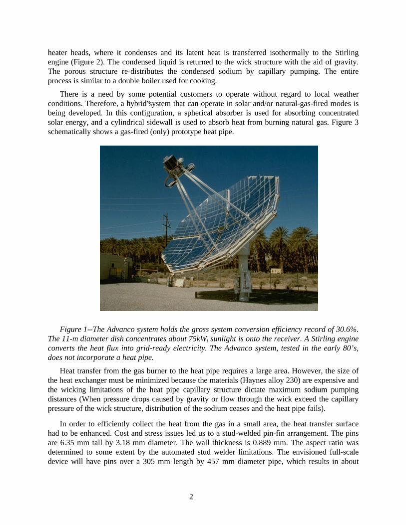
Figure 1--The Advanco system holds the gross system conversion efficiency record of 30.6%. About 75kWt sunlightis concentrated by the 11-m diameter dish onto the receiver. A Stirling engine converts the heat flux intogrid-ready electricity. The Advanco system, tested in the early 80’s, does not incorporate a heat pipe..... 2

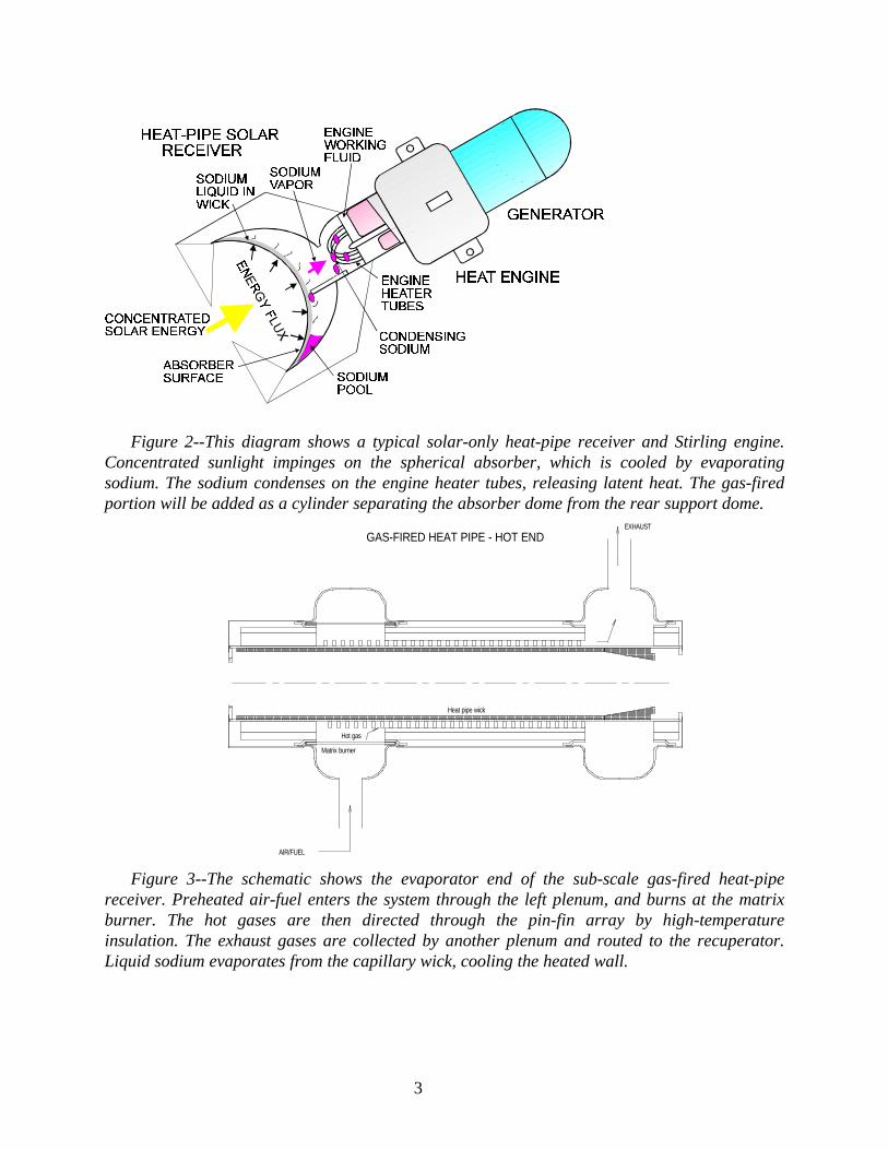
Figure 2--This diagram shows a typical solar-only heat-pipe receiver and Stirling engine. Concentrated sunlightimpinges on the spherical absorber, which is cooled by evaporating sodium. The sodium condenses on theengine heater tubes, releasing latent heat. The gas-fired portion will be added as a cylinder separatingthe absorber dome from the rear support dome. ....................................................................................... 3

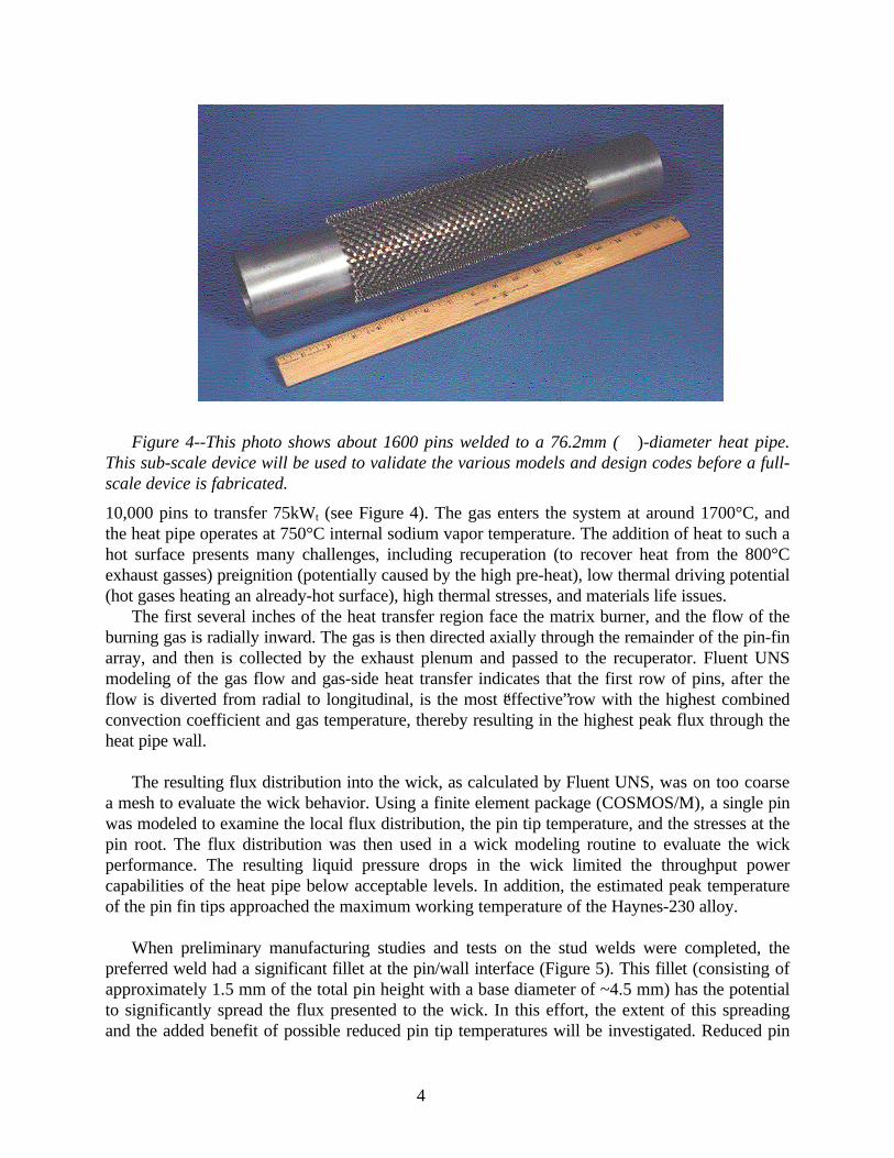
Figure 3--The schematic shows the evaporator end of the sub-scale gas-fired heat-pipe receiver. Preheated air-fuel enters the system through the left plenum, and burns at the matrix burner. The hot gases are thendirected through the pin-fin array by high-temperature insulation. The exhaust gases are collected byanother plenum and routed to the recuperator. Liquid sodium evaporates from the capillary wick, coolingthe heated wall......................................................................................................................................... 3

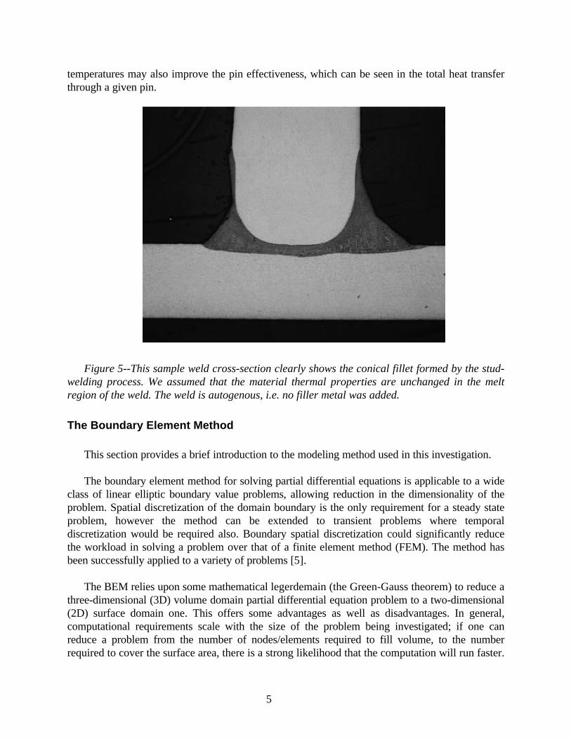
Figure 4--This photo shows about 1600 pins welded to a 76.2mm (3”)-diameter heat pipe. This sub-scale devicewill be used to validate the various models and design codes before a full-scale device is fabricated....... 4

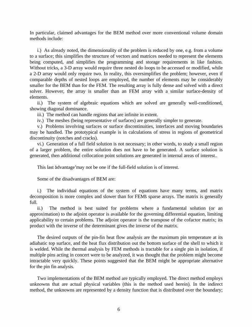
Figure 5--This sample weld cross-section clearly shows the conical fillet formed by the stud-welding process. Weassumed that the material thermal properties are unchanged in the melt region of the weld. The weld isautogenous, i.e. no filler metal was added.............................................................................................. 5

Figure 6--Local node numbering for a nine node continuous quadrilateral element............................................. 11

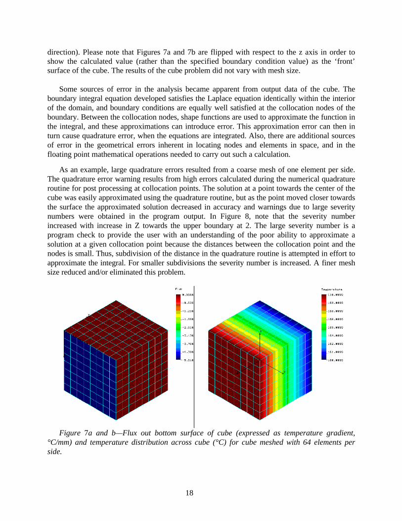
Figure 7a and b—Flux out bottom surface of cube (expressed as temperature gradient, °C/mm) and temperaturedistribution across cube (°C) for cube meshed with 64 elements per side. .............................................. 18

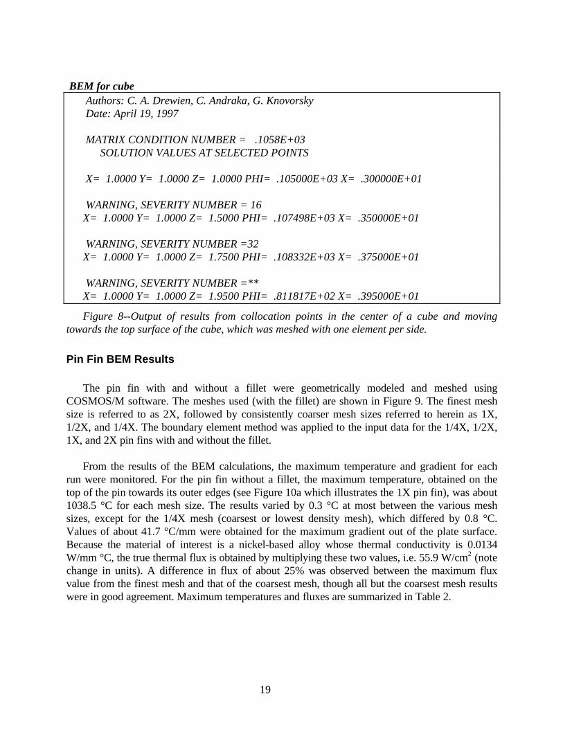
Figure 8--Output of results from collocation points in the center of a cube and moving towards the top surface ofthe cube, which was meshed with one element per side. ......................................................................... 19

Figure 9a. --BEM meshes of the 2X filleted pin fin model. .................................................................................. 20

Figure 10 a and b—Temperature and gradient distribution for the straight pin fin (1X)...................................... 22

Figure 11--a.) Temperature distribution for the 2X filleted pin fin (°C). b.) Gradient distribution for the 2Xfilleted pin fin (°C/mm). ......................................................................................................................... 22

Figure 12--Variation in BEM-calculated heat flux distribution for filleted and straight pin fins with respect tomesh density........................................................................................................................................... 24

Figure 13--a.) 1X FEM and 1/2X FEM mesh (20 nodes/element & 8 nodes/element, respectively) and b.) 1/4XFEM mesh.............................................................................................................................................. 25

Figure 14--Heat flux in z direction (W/mm2) and Temperature(°C) distributions calculated by FEM for a.) 1X, b.)1/2X, and c.) 1/4X meshes. ..................................................................................................................... 27

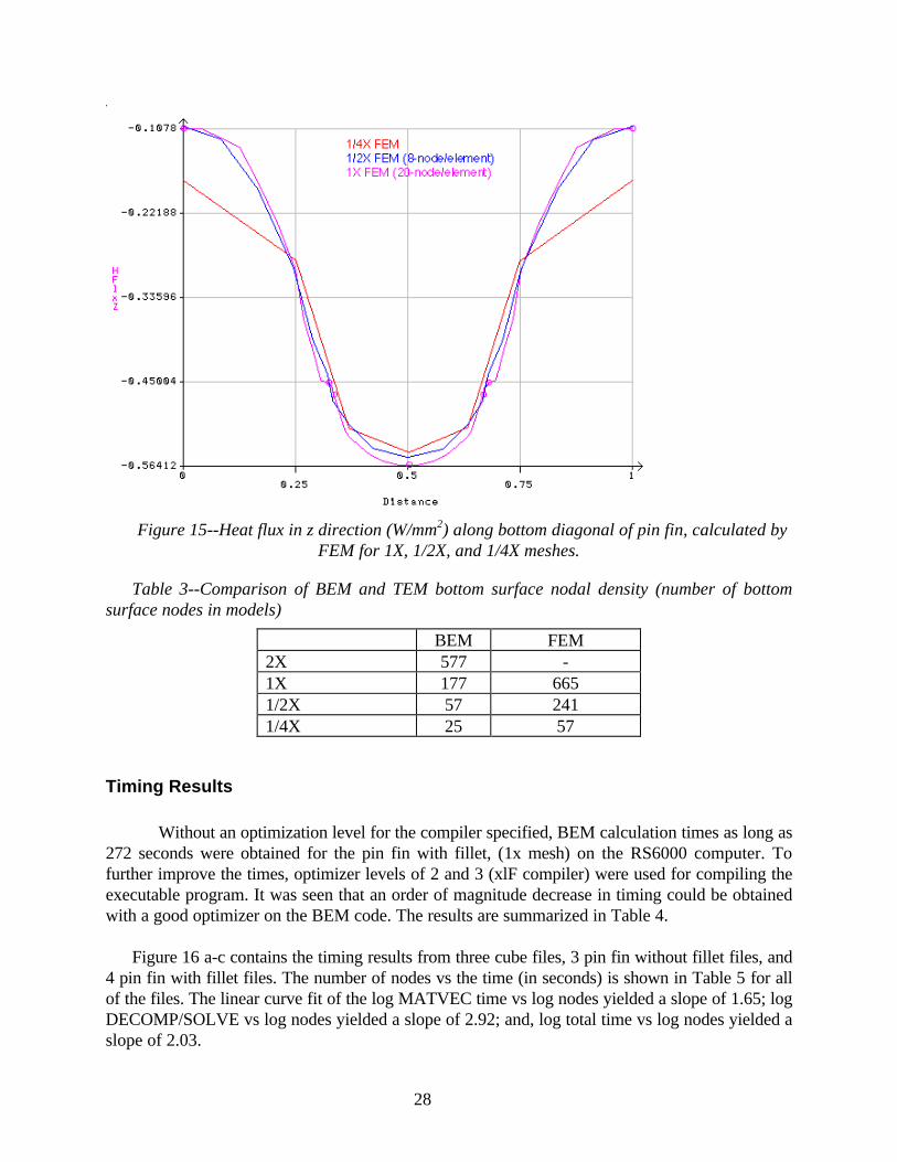
Figure 15--Heat flux in z direction (W/mm2) along bottom diagonal of pin fin, calculated by FEM for 1X, 1/2X,and 1/4X meshes. ................................................................................................................................... 28

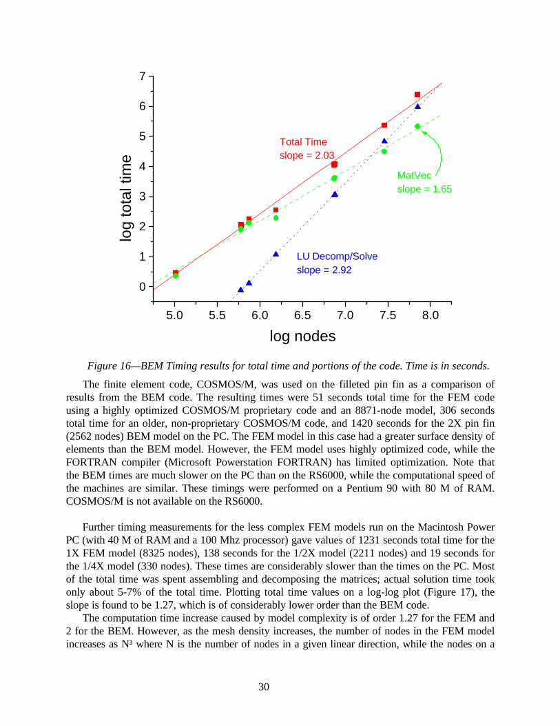
Figure 16—BEM Timing results for total time and portions of the code. Time is in seconds................................. 30

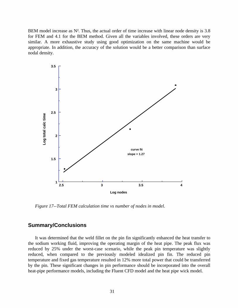
Figure 17--Total FEM calculation time vs number of nodes in model. ................................................................. 31

iii

List of Tables

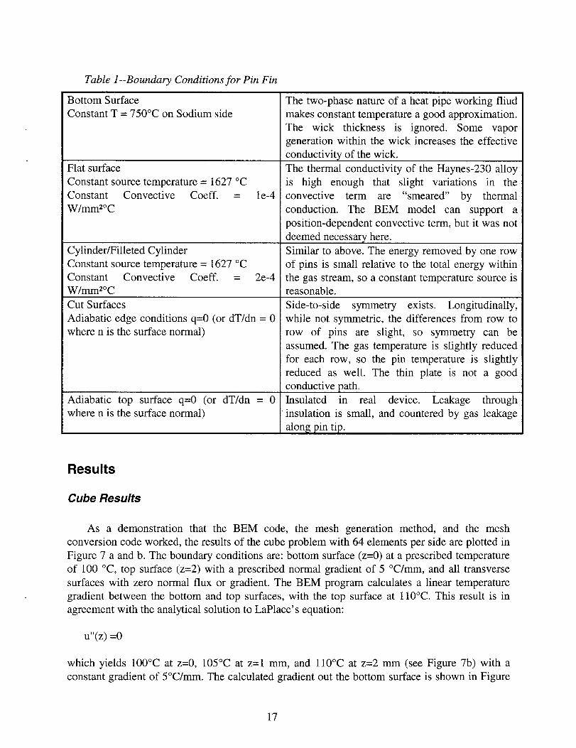
Table 1--Boundary Conditions for Pin Fin........................................................................................................... 17

Table 2--Peak temperature and flux with mesh density. The results are for the BEM model except as noted. ....... 24

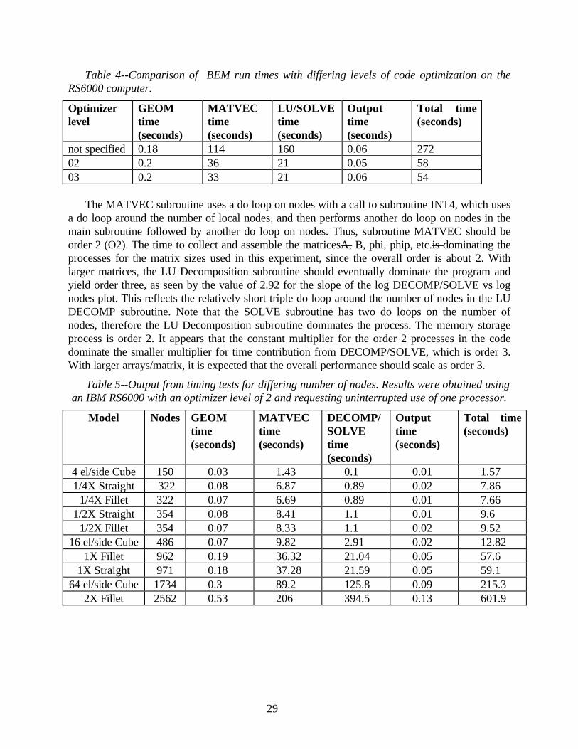
Table 3--Comparison of BEM and TEM bottom surface nodal density (number of bottom surface nodes in models)28

Table 4--Comparison of BEM run times with differing levels of code optimization on the RS6000 computer....... 29

Table 5--Output from timing tests for differing number of nodes. Results were obtained using an IBM RS6000 withan optimizer level of 2 and requesting uninterrupted use of one processor. ............................................ 29

1

Introduction

In this project, we model the thermal conduction of a portion of an enhanced-surface heatexchanger for a gas-fired heat pipe solar receiver. The surface enhancement is accomplished byan array of pin fins on the gas-fired side of the heat exchanger. In prior work, the heat exchangerassembly was modeled in Fluent UNS, a commercial computational fluid dynamics code[1], todetermine the hot gas flow field over the pin fin array. The Fluent modeling indicated high localthermal flux at several pin rows. The results of the Fluent modeling (gas temperature andconvection coefficient) were used in a finite element program (COSMOS/M, v1.75)[2] todetermine the stresses and heat transfer at the critical pin fin in much greater detail. The calculatedthermal flux and peak pin-tip temperatures were sufficiently high to cause concern for the unit’sservice life.

Since then, weld procedures have been developed and refined in order to get consistentautomated welds of the pin fins to the wall material. The resulting weld has a conical fillet aroundthe base of the pin, which was not included in the original modeling. The purpose of the currentwork is to determine the relative effect of this fillet on the heat transfer characteristics of the pin.In particular, we are interested in the effect on the peak pin temperature (materials limitations)and on the local flux distribution into the heat pipe wick (wick limitation).

Since all of the areas of interest lie on the outer surfaces, or boundaries, of the pin structure,we do not need a full-field solution such as given by finite element methods (FEM). Therefore,this problem would seem to be natural match for the boundary element method (BEM).

In solving this heat transfer problem, we develop a process that could be utilized by others fordesigning the surface mesh on an object of interest, performing a conversion from the mesh intothe input format utilized by the BEM code [3], obtaining output on the surface of the object, anddisplaying visual results. The process was first tried on a simple cube with known analyticsolution. Once the process was established, it was applied to the pin fins. The performance of theBEM program on the pin fin was measured (as computational time) and used as a performancecomparison with the FEM model. The approach and process are presented here, and can be usedfor application to similar problems.

Background

The Heat Exchanger and Pin Fin

The heat pipe receiver is a component of a solar thermal heat receiver for a dish-Stirlingelectric generation system. In solar-only operation, a heat pipe acts as a “heat transformer,”accepting the non-uniform concentrated sunlight from a parabolic dish and transferring the heatuniformly and isothermally to a Stirling engine (Figure 1)[4]. The inside surface of the heat pipeabsorber is covered with a porous structure saturated with liquid sodium. The heat pipe enclosureis evacuated. The concentrated solar flux is absorbed through the absorber surface, evaporatingthe sodium, which limits the absorber surface temperature. The vapor generated flows to the

2

heater heads, where it condenses and its latent heat is transferred isothermally to the Stirlingengine (Figure 2). The condensed liquid is returned to the wick structure with the aid of gravity.The porous structure re-distributes the condensed sodium by capillary pumping. The entireprocess is similar to a double boiler used for cooking.

There is a need by some potential customers to operate without regard to local weatherconditions. Therefore, a “hybrid” system that can operate in solar and/or natural-gas-fired modes isbeing developed. In this configuration, a spherical absorber is used for absorbing concentratedsolar energy, and a cylindrical sidewall is used to absorb heat from burning natural gas. Figure 3schematically shows a gas-fired (only) prototype heat pipe.

Figure 1--The Advanco system holds the gross system conversion efficiency record of 30.6%.The 11-m diameter dish concentrates about 75kWt sunlight is onto the receiver. A Stirling engineconverts the heat flux into grid-ready electricity. The Advanco system, tested in the early 80’s,does not incorporate a heat pipe.

Heat transfer from the gas burner to the heat pipe requires a large area. However, the size ofthe heat exchanger must be minimized because the materials (Haynes alloy 230) are expensive andthe wicking limitations of the heat pipe capillary structure dictate maximum sodium pumpingdistances (When pressure drops caused by gravity or flow through the wick exceed the capillarypressure of the wick structure, distribution of the sodium ceases and the heat pipe fails).

In order to efficiently collect the heat from the gas in a small area, the heat transfer surfacehad to be enhanced. Cost and stress issues led us to a stud-welded pin-fin arrangement. The pinsare 6.35 mm tall by 3.18 mm diameter. The wall thickness is 0.889 mm. The aspect ratio wasdetermined to some extent by the automated stud welder limitations. The envisioned full-scaledevice will have pins over a 305 mm length by 457 mm diameter pipe, which results in about

3

Figure 2--This diagram shows a typical solar-only heat-pipe receiver and Stirling engine.Concentrated sunlight impinges on the spherical absorber, which is cooled by evaporatingsodium. The sodium condenses on the engine heater tubes, releasing latent heat. The gas-firedportion will be added as a cylinder separating the absorber dome from the rear support dome.

GAS-FIRED HEAT PIPE - HOT END

Heat pipe wick

AIR/FUEL

Matrix burner

Hot gas

EXHAUST

Figure 3--The schematic shows the evaporator end of the sub-scale gas-fired heat-pipereceiver. Preheated air-fuel enters the system through the left plenum, and burns at the matrixburner. The hot gases are then directed through the pin-fin array by high-temperatureinsulation. The exhaust gases are collected by another plenum and routed to the recuperator.Liquid sodium evaporates from the capillary wick, cooling the heated wall.

4

Figure 4--This photo shows about 1600 pins welded to a 76.2mm ( )-diameter heat pipe.This sub-scale device will be used to validate the various models and design codes before a full-scale device is fabricated.

10,000 pins to transfer 75kWt (see Figure 4). The gas enters the system at around 1700°C, andthe heat pipe operates at 750°C internal sodium vapor temperature. The addition of heat to such ahot surface presents many challenges, including recuperation (to recover heat from the 800°Cexhaust gasses) preignition (potentially caused by the high pre-heat), low thermal driving potential(hot gases heating an already-hot surface), high thermal stresses, and materials life issues.

The first several inches of the heat transfer region face the matrix burner, and the flow of theburning gas is radially inward. The gas is then directed axially through the remainder of the pin-finarray, and then is collected by the exhaust plenum and passed to the recuperator. Fluent UNSmodeling of the gas flow and gas-side heat transfer indicates that the first row of pins, after theflow is diverted from radial to longitudinal, is the most “effective” row with the highest combinedconvection coefficient and gas temperature, thereby resulting in the highest peak flux through theheat pipe wall.

The resulting flux distribution into the wick, as calculated by Fluent UNS, was on too coarsea mesh to evaluate the wick behavior. Using a finite element package (COSMOS/M), a single pinwas modeled to examine the local flux distribution, the pin tip temperature, and the stresses at thepin root. The flux distribution was then used in a wick modeling routine to evaluate the wickperformance. The resulting liquid pressure drops in the wick limited the throughput powercapabilities of the heat pipe below acceptable levels. In addition, the estimated peak temperatureof the pin fin tips approached the maximum working temperature of the Haynes-230 alloy.

When preliminary manufacturing studies and tests on the stud welds were completed, thepreferred weld had a significant fillet at the pin/wall interface (Figure 5). This fillet (consisting ofapproximately 1.5 mm of the total pin height with a base diameter of ~4.5 mm) has the potentialto significantly spread the flux presented to the wick. In this effort, the extent of this spreadingand the added benefit of possible reduced pin tip temperatures will be investigated. Reduced pin

5

temperatures may also improve the pin effectiveness, which can be seen in the total heat transferthrough a given pin.

Figure 5--This sample weld cross-section clearly shows the conical fillet formed by the stud-welding process. We assumed that the material thermal properties are unchanged in the meltregion of the weld. The weld is autogenous, i.e. no filler metal was added.

The Boundary Element Method

This section provides a brief introduction to the modeling method used in this investigation.

The boundary element method for solving partial differential equations is applicable to a wideclass of linear elliptic boundary value problems, allowing reduction in the dimensionality of theproblem. Spatial discretization of the domain boundary is the only requirement for a steady stateproblem, however the method can be extended to transient problems where temporaldiscretization would be required also. Boundary spatial discretization could significantly reducethe workload in solving a problem over that of a finite element method (FEM). The method hasbeen successfully applied to a variety of problems [5].

The BEM relies upon some mathematical legerdemain (the Green-Gauss theorem) to reduce athree-dimensional (3D) volume domain partial differential equation problem to a two-dimensional(2D) surface domain one. This offers some advantages as well as disadvantages. In general,computational requirements scale with the size of the problem being investigated; if one canreduce a problem from the number of nodes/elements required to fill volume, to the numberrequired to cover the surface area, there is a strong likelihood that the computation will run faster.

6

In particular, claimed advantages for the BEM method over more conventional volume domainmethods include:

i.) As already noted, the dimensionality of the problem is reduced by one, e.g. from a volumeto a surface; this simplifies the structure of vectors and matrices needed to represent the elementsbeing computed, and simplifies the programming and storage requirements in like fashion.Without tricks, a 3-D array would require three nested do loops to be accessed or modified, whilea 2-D array would only require two. In reality, this oversimplifies the problem; however, even ifcomparable depths of nested loops are employed, the number of elements may be considerablysmaller for the BEM than for the FEM. The resulting array is fully dense and solved with a directsolver. However, the array is smaller than an FEM array with a similar surface-density ofelements.

ii.) The system of algebraic equations which are solved are generally well-conditioned,showing diagonal dominance.

iii.) The method can handle regions that are infinite in extent.iv.) The meshes (being representative of surfaces) are generally simpler to generate.v.) Problems involving surfaces or surface discontinuities, interfaces and moving boundaries

may be handled. The prototypical example is in calculations of stress in regions of geometricaldiscontinuity (notches and cracks).

vi.) Generation of a full field solution is not necessary; in other words, to study a small regionof a larger problem, the entire solution does not have to be generated. A surface solution isgenerated, then additional collocation point solutions are generated in internal areas of interest..

This last ‘advantage’ may not be one if the full-field solution is of interest.

Some of the disadvantages of BEM are:

i.) The individual equations of the system of equations have many terms, and matrixdecomposition is more complex and slower than for FEM’s sparse arrays. The matrix is generallyfull.

ii.) The method is best suited for problems where a fundamental solution (or anapproximation) to the adjoint operator is available for the governing differential equation, limitingapplicability to certain problems. The adjoint operator is the transpose of the cofactor matrix; itsproduct with the inverse of the determinant gives the inverse of the matrix.

The desired outputs of the pin-fin heat flow analysis are the maximum pin temperature at itsadiabatic top surface, and the heat flux distribution out the bottom surface of the shell to which itis welded. While the thermal analysis by FEM methods is tractable for a single pin in isolation, ifmultiple pins acting in concert were to be analyzed, it was thought that the problem might becomeintractable very quickly. These points suggested that the BEM might be appropriate alternativefor the pin fin analysis.

Two implementations of the BEM method are typically employed. The direct method employsunknowns that are actual physical variables (this is the method used herein). In the indirectmethod, the unknowns are represented by a density function that is distributed over the boundary;

7

this does not lend itself to physical interpretation. However, once the density function has beendetermined completely, physical variables can be deduced.

This latter method leads to the last disadvantage of the BEM approach; it can be difficult tounderstand! Unlike the Finite Difference (FD) and FEM approaches, which are basicallystraightforward, this method relies upon some abstract mathematical foundations. Thus,qualitatively comparing the algorithms used to set up the matrix from which solutions arecalculated, the FD approach is easy, the FEM approach is moderately easy, and the BEM isdifficult. While using an already written code goes a long way to alleviate this problem, whenproblems are encountered, as they inevitably will be, debugging becomes difficult. Thus, theapproach here was to start small and simple as described below.

Purpose

The goals of this investigation were to determine the following:

• What are the thermal flux and temperature distributions on the pin fin?• How did the weld fillet influence the heat transfer in the pin fin (What is the effect of the weld

geometry vs. the idealized cylindrical pin)?• Is there any thermal performance gain realized by the fillet on the actual welded pin fin?• Are there significant computational speed advantages for the BEM over the FEM approach?• How do the BEM results compare with the FEM results?• What level of mesh size could be used to obtain reasonable results for BEM vs FEM?

What was the order of the calculation relative to the number of nodes in the mesh?

Approach

Project Plan

In order to apply the boundary element method to the pin fin problem, the following tasks hadto be accomplished:

i.) Obtain BEM steady state code. ii.) Get code to run. iii.) Determine method to build mesh for pin fin. We knew that the original FEM mesh used

in the stress analysis for the pin fin had about 10,000 nodes, so this had to be anautomated method.

iv.) Determine method to apply boundary conditions (BC’s) to the meshed object. v.) Determine method to produce appropriate input file for the BEM code. The BEM

program needed to have a particular data structure linking local and globalrepresentations of the nodes. It also needed to have data in a particular format.

8

vi.) Determine method to extract data from code output files. The normal method is to usecollocation nodes which are interior to the domain. Since we were looking on the surface,the results were calculated directly, but were not transparent without some further codemodification.

vii.) Determine method to plot data. Interpretation of large data structures is difficult withouta suitable visualization tool. In the case of the heat flow problem, direct visualization ofthe temperatures and heat fluxes superimposed on the actual part is the moststraightforward way.

BEM 3D Steady State Code

The boundary element code, npot3d.f, was developed by Marc Ingber [3], University of NewMexico. The code is written in Fortran77. For this investigation, it was run using an xlf compileron the IBM RS6000 computer in addition to the comparison testing with the FEM model whichwas performed on a desktop computer. The code in its present form contains very little internaldocumentation, but two reports for input file format [6] and boundary element formulation andprogram description for the transient heat conduction problem[5] exist. A brief overview of theprogram (listing provided in Appendix A) follows.

The main program initializes variables, constants, and the input file name. All arrays aredimensioned. The input file and output files are opened. Then the subroutines QUADR, GEOM,MATVEC, DECOMP, SOLVE, and CALPHI are called before final data is output and theprogram ends.

Subroutine GEOM reads data from the input file:

Titleswhether the domain is interior or exteriornumber of additional collocation points chosen outside of the domainnumber of nodesnumber of elementsnode numberx, y, and z coordinatesboundary condition value and typelocal node to global nodenumber of collocation pointsx, y, and z coordinates of collocation points for obtaining an approximate solution.

Subroutine MATVEC collects and assembles vectors and matrix A. It sets up collocationpoints based upon the interior or exterior of the domain and then calls Subroutine INT4 tointegrate the Green’s integrals. On return the A matrix and B vector are filled in based uponwhether temperature or flux or both were specified for the boundary condition. The A matrix isfilled utilizing Ah1 and Ah2 vectors. The B vector is filled using B, Phi, Ah1, and Ah2 vectors.

9

Subroutine INT4 identifies coordinates based upon element type--triangular or quadrilateral.It calculates the distance of the surface collocation point to the surrounding local nodes, sets thevalue of “inode” based upon that distance relative to small (1e-6) and then calls subroutineRQINT for a quadrilateral element type. On return G1 and G1P values are available forcalculation of the Ah1 and Ah2 vectors.

Subroutine RQINT is book keeping in nature. If the element type is continuous quadrilateralthen subroutine RQINTC is called, otherwise RQINTD is called for the discontinuousquadrilateral element.

Subroutine RQINTC finds the longest diagonal of the element (H), then finds the distancefrom the surface collocation point to the center of the element (D). The severity is H/D. Thus, thesmaller the distance D, the larger the severity value. If the severity value is less than 0.358, thenthe severity number is 1, otherwise subroutine DER9T is called. If DER9T is called, then a newdistance is calculated based upon use of a smaller sub-spacing during quadrature. Effectively, thederivative times the coordinates are summed to find a new gauss point. The normal to the elementsurface (q) is found and converted to a unit normal vector (u) in subroutine UNORMAL. Onreturn the dot product of u with the vector from the element center to the collocation point isperformed to find the angle between the two vectors. A new severity number is calculated and awarning is sent if the severity number is greater than 9. DER9T is called again and gaussweighting is used for the distance determination. The surface normal and its unit vector arecalculated and then subroutine FUNDS is called. On return from FUNDS, G1 and G1P vectorsare formed before returning to INT4.

Subroutine DER9T is the derivative of the shape function for the 9 local node quadrilateralelement.

Subroutine UNORMAL calculates the surface normal to the element (q) and its unit vector(u).

Subroutine DER9TD returns the derivative of the shape function for the discontinuouselement.

Subroutine FUNDS calls the appropriate shape function routine based upon the element type.For the continuous quadrilateral, SH9T is shape function for the 9 node continuous quadrilateralelement.

Subroutine DECOMP is a matrix decomposition routine using LU decomposition.

Subroutine SOLVE uses back substitution to solve the linear algebra equation. Here matrix Aand vector B are used to find the solution vector.

Subroutine CALPHI calculates the approximate solution at the collocation points of interestto the program user. This routine was not utilized for this work because only answers on the

10

surface were of interest; the answers were either in the specified boundary condition vectors oreasily obtained from the solution vector.

Code Modifications

Some modifications to the npot3d.f code were performed to facilitate use on this project (seeAppendix A). These modifications are summarized as follows:

i.) Several “OPEN” statements were added in order to output particular data to separate files.Output of the solution vector and the boundary conditions were combined to form an output filecalled *.plt, which contains columns of "Node", "Temperature", and "Flux". Another output filewas created for the timing operations that were added to the program; this output file is *.tim andcontains readable lines of code with the time specified by the machine (here in seconds). Theoutput file *.out outputs "x", "y", and "z" coordinates along with "Temperature". This is thestandard output file that would result from input of collocation points. This file may be useful tosome users if collocation points are desired. Alternately, the slight difference in the *.plt and *.outfiles is based upon the ability to plot in 3 dimensions. The plotting routine employed in this effortwas the COSMOS/M program that was used to generate the mesh; the surface was defined by thenode number and visual output was easily obtained from the *.plt file.

ii.) A “READ” statement for keyboard entry of the name of the input file was added. Thisfeature is optional and can easily be commented out: root, the filename without the extension issimply assigned the 'filename'. Note the filename has to be 8 characters long. For batch-modetiming tests with llsubmit (see next section), this name had to be entered prior to execution andthese two lines had to be commented out of the code.

iii.) Timing was added to the program in order to see the influence of mesh size on the timerequired by the various subroutines--MATVEC, GEOM, DECOMP/SOLVE, and CALPHI. Thetotal time was also reported. Timing was performed using the mytime.f program[6].

iv.) The pointers to the first element in an array were specified as “array(1)” in the dimensionstatements of the subroutines. The xlf compiler does not accept this notation and the "1" waschanged to an "*" in order to specify the pointer and not indicate an array size of 1.

v.) Array dimensions were initially set to 600 for the matrix, forcing vector, and solutionvector in addition to many other arrays that relied upon the number of elements. The arraydimensions were changed to 4000 to accommodate the size of the input meshes used in this work.

vi.) Comments were added to aid future users.

Timing Tests

Timing tests were run using npot3d.f with mytime.f [7] on an IBM RS6000 computer.Originally, no optimizer level was specified and timing was performed without requestinguninterrupted use of one node of the machine. Next, the timing tests were rerun using the samefiles but requesting uninterrupted use of one node of an IBM SP1 computer (one node is identicalto the RS6000) through the llsubmit command. A command file (*.cmd) was formulated in which

11

the *.in and *.out were not designated because the npot3d.f code opens standard input (unit 5)and output (unit 6) during the execution. Timing was performed for the total run time and thesubroutines GEOM, MATVEC, DECOMP/SOLVE, and CALPHI and writing to output files.Note that the time around both the DECOMP and SOLVE subroutines was combined into oneinterval. Some timing results were also supplied as standard output of the COSMOS/M FEMcode.

Mesh Description

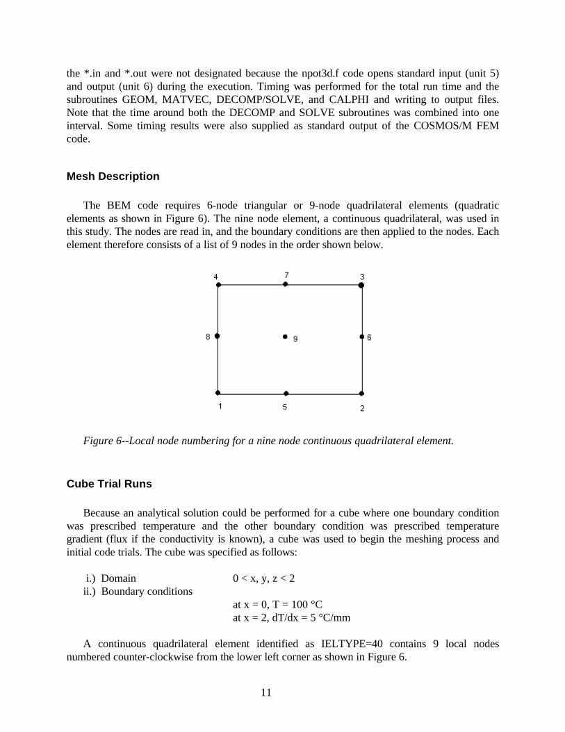
The BEM code requires 6-node triangular or 9-node quadrilateral elements (quadraticelements as shown in Figure 6). The nine node element, a continuous quadrilateral, was used inthis study. The nodes are read in, and the boundary conditions are then applied to the nodes. Eachelement therefore consists of a list of 9 nodes in the order shown below.

Figure 6--Local node numbering for a nine node continuous quadrilateral element.

Cube Trial Runs

Because an analytical solution could be performed for a cube where one boundary conditionwas prescribed temperature and the other boundary condition was prescribed temperaturegradient (flux if the conductivity is known), a cube was used to begin the meshing process andinitial code trials. The cube was specified as follows:

i.) Domain 0 < x, y, z < 2ii.) Boundary conditions

at x = 0, T = 100 °C at x = 2, dT/dx = 5 °C/mm

A continuous quadrilateral element identified as IELTYPE=40 contains 9 local nodesnumbered counter-clockwise from the lower left corner as shown in Figure 6.

12

For the cube we started with a simple mesh which had 6 elements (one per cube face). Thiswas generated by hand. Mesh element area was then decreased by factors of 4. Eventually, cubemeshes were generated with 4, 16, 64 and 256 elements per face. Results were calculated for upto 64 elements per face.

The overall process was defined during implementation of the cube. Briefly, the input file wasformed by employing COSMOS/M mesh generating software. The global node, x,y, and zcoordinates, and the local node number were derived from this software package. Next, aconversion of this data into the input format for npot3d.f was performed using a conversionprogram. This conversion program forms the file into the format described in Ingber[6]. Initialtrials of the input file resulted in erroneous output (vs. the known analytical solution). It wasdetermined that certain elements were indexed in a clockwise fashion and/or the combining ofelements to form the cube resulted in inside-out placement of an element. Therefore, theconversion program was adapted to check for this error. If the surface normal for all elementspointed into the cube such that the numbering of local nodes is in the counter-clockwise mannerspecified, the elements combined together in the proper manner. Rerunning the code after theconversion program implemented checking and correction for this error, the correct results wereobtained.

Mesh Generation

The tool used for mesh generation, GEOSTAR, is part of a commercial FEM packageCOSMOS/M [2]. Like all such packages, it is comprised of a three dimensional solid modeler plusfacilities for associating a variety of elements with the solid geometric models. Fortunately, thelibrary of elements included a nine-node shell element that provided most of the characteristicsneeded for the BEM code. Activities involving the GEOSTAR code were run on a MacintoshPowerPC 8100/100. Files generated were then handed off via electronic mail to a CompaqPressario 1080, where a file conversion package written in C++ was used to convert them to aformat appropriate for the BEM code. The code was run on a variety of platforms including theIBM RS6000, the same Compaq used to convert the GEOSTAR files, and on a Pentium baseddesktop computer where the original FEM work was completed to give a better relativecomputational time comparison. FEM runs of less complex meshes were also run on theMacintosh PowerPC 8100/100.

The general procedure in developing the mesh involved:

i.) Generating a geometric model based upon key points, curves between the key points, andfinally surfaces defined by the curves.

ii.) Once these surfaces were defined, elements and their underlying nodes could begenerated. Normally, a material group and its associated physical properties are defined beforemeshing a group of elements. This was not strictly necessary for this problem, since the full FEMpackage was not going to be used, however, it was found convenient to do so in order to markelements with an identifier that would enable their easy selection based upon the differing types ofboundary conditions to be added later.

13

iii.) Because some of the surfaces were generated by parallel replication of already existingsurfaces, their surface normal was not always consistent relative to inside vs outside the pin fin.An example would be the inside vs the outside surface of the shell, or opposite cut edges of theshell. Hence the elements which were subsequently generated on generated areas were notnecessarily oriented correctly to give the counterclockwise nodal numbering scheme expected bythe BEM code. Two approaches were used to rectify this situation. The first was to use the fileconversion code, and the second was to determine the orientation of selected elements on asurface (all the nodal numbering sequences on a given surface were consistently numbered) bylooking up the nodes associated with a given element and noting whether they were correctlyordered. Needless to say this was somewhat laborious. An alternative was found as part ofactivities associated with figuring out how to plot the data output by the BEM code. As part ofthat activity, it was desirable to generate an output file for a pin fin model so we could replicate itsstructure. A simple thermal model was built, and it was found that the 9-node shell element wasnot compatible with a thermal heat flow analysis (though it would allow thermal loading todetermine expansion/contraction ). Wishing to generate an output file and not having any other 9-pt elements, the simplest alternative loading was tried, that of applying a hydrostatic pressure. Itwas then noticed that the vector arrows used to indicate the pressure loading were pointingoutward on those elements which needed to be flipped, and pointing inward on those which werecorrect. Once these elements were identified, COSMOS/M provides a simple command whichallows inverting their ‘direction’. Thereafter, this approach was applied before moving on to thenext operation.

iv.) After the individual groups were identified by nodal and elemental numbers, nodalmerging was accomplished. This basically merged collocated nodes on adjacent surfaces whichdid not have differing boundary conditions. On those common boundaries where the boundaryconditions did change, this was not done. The operation of merging could be done exclusivelybetween nodes of a single material group, by issuing a command letting them merge only amongnodes of their own group. Once the merging operation was completed, a renumbering(compression) operation was performed to renumber the nodes consecutively and fill in the spacesleft by those nodes, which had been subtracted by the nodal merge operation. A listing of a typicalCOSMOS/M session file is included in Appendix B.

Mesh Conversion

As noted, COSMOS/M has automatic mesh-generation tools that proved simple to use formesh generation over the cube or pin fin surface, and provided quadratic 9-node shell elements, asrequired by the BEM code (see Figure 6). However, the FEM model grouped the elements byboundary condition, rather than nodes.

A conversion routine (see Appendix C) was formulated in C++ to convert the FEM model tothe BEM input file format. This C++ code, referred to herein as the mesh converter, reads all ofthe nodes and elements from the COSMOS/M nodel/element list file into memory, crossreferences the nodes and elements, and prints them in the proper BEM format. The code alsoprompts the user for the boundary conditions, and performs limited data validation. The datavalidation includes searching for backward elements and checking for conflicting boundaryconditions. Two elements can share the same node only if the elements have the same boundary

14

conditions. If differing boundary conditions are desired, the node must be duplicated rather thanshared. A warning is given, and the first boundary condition is applied. The mesh converter doesnot fix warnings of this type; a return to COSMOS/M is necessary. Duplicate nodes shouldalways be used when the boundary conditions are not continuous (i.e., at an edge).

As noted above, early in this program a significant problem encountered was the difficulty indetermining if all of the elements were numbered in the correct order (counter-clockwise asshown in Figure 6 rather than clockwise), i.e. that all of the surface normals were outward.Eventually, the method described in the previous section (using GEOSTAR and pressureloading) was used to solve this problem. However, an alternative method was written into themesh conversion program (and which subsequently served as a check on the GEOSTARprocedure).

The first step in this validation is to find the center of “mass” of the nodes, by simply averagingtheir locations. Then, two vectors are formed on the surface of the element, one from the centernode (9) of the element to the first node (1), and one from the center to the second node (2). Thecross product of these vectors creates a normal vector. Then the dot product of this normal and avector from the center of mass to the center of the element is determined. If the dot product ispositive, the normal is pointing away form the center of mass. In the case of the pin fin assembly,some correctly-pointing elements (top face of the flat plate) gave negative dot products becausethe center of mass was too high in the pin. Therefore, the user can input an alternative center forchecking. A “hidden” and potentially dangerous feature is the capability to reverse these backwardelements. This feature is accessed by pressing a lower-case f (for “fix”) when prompted whether anew center location is desired. Then, any elements found to be backward when compared to thenew center will be repaired. It is safer to use the conversion program’s feedback and actuallyrepair the model in COSMOS/M instead. There the graphical results can be examined for errorsbefore proceeding to the next step.

The conversion routine is also used to apply the boundary conditions to the nodes. The nodesare associated with elements, and the elements are grouped by COSMOS/M for differentboundary conditions. The possible choices are specified temperature (nbdy=1), specifiedtemperature gradient (nbdy=2), and mixed, or convection, conditions (nbdy=3). If a flux isspecified, it must be divided by the material conductivity (k) to get a temperature gradient. Forconvection boundary conditions, the BEM method uses the following equation:

φ(x) + β(x)φ′(x) = γ(x)where:

φ is the process variable (Temperature in our case)φ’ is dφ/dx

In a heat transfer problem, β is k/h where h is the convective coefficient and γ is the free-stream temperature of the gas. The gradient ( φ’ ) can be expressed as a flux by multiplying by thethermal conductivity of the material modeled. The converter routine prompts for each parameterfor each element group, using free-form (white space-delimited) input.

15

As can be seen in the code in Appendix C, the conversion routine is implemented as threeclasses. The first two are an element class and a node class. Arrays of these items are stored in thethird “model” class. Operations included allow cross-referencing, reading, and outputting the nodesand elements. The model contains allocable arrays of nodes and elements, so the permissible sizeof the nodal arrays is limited only by available memory.

Data VisualizationAn initial attempt was made to display the results of the BEM calculation using MatLab[8];

while MatLab is a very powerful package for scientific and engineering calculations and theirdisplay, it is also a package with a steep learning curve. The basic problem with it seemed to bethat while results could be plotted in 3D with pre-loaded function calls, they needed to be on auniform grid, and the nodal points (and results) were not on such a grid. Further, piecing together(or displaying separately) the several parts of the pin fin was difficult, although easy for the cube.Therefore, other methods were sought.

Several other packages (including Mathematica[9]) were considered before it was realizedthat the best approach was to use the plotting routines inherent to the mesh generation package.The COSMOS/M user-provided data plotting facility offered two options. One could either enternode-defined inputs or element-defined inputs. The nodal approach actually is still plotted onelements (more about this later), but when a nodal approach is chosen, the values plotted acrossthe elements are interpolated between the nodal values. In contrast, when the elemental approachis used, the elements show only a single value. Thus the result has a mosaic like pattern. Thenodal viewpoint is better for some approaches and was desirable because nodal temperatures (theoutput of the BEM code) were of interest. The elemental approach also has its benefits, primarilyin displaying boundary conditions that are element related. In the data file structure a flag was tobe set which would tell the plotting routine which was desired. The documentation had this flagreversed.

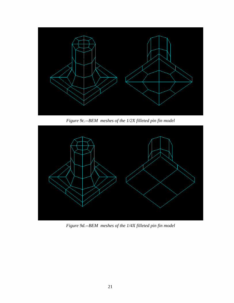
As noted above, the nodal results are plotted in an elemental manner using internodalinterpolation. One additional observation is that the elements are plotted as planes, even if theelements are not planar. This only occurs when higher order elements (such as the 9-nodeelement) are used. It is probable that the plotting routine was developed for square or triangular 4and 3 node elements. The net effect is that while the non-corner nodes for the cylindrical portionsof the pin fin are actually on a cylindrical surface, they are represented as being polygonal. Thisonly becomes evident on relatively coarse meshes, such as the 1/2 and 1/4 mesh models.

Pin Fin Analysis

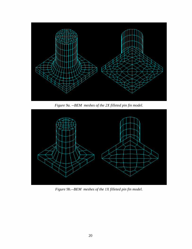
A nominal mesh size was selected for the first BEM pin fin model, with about 970 surfacenodes. Additional meshes of greater and lesser nodal densities were used, with a total span of 16:1in mesh density. The nominal model is referred to as the 1X model. The additional models werelabeled 1/4X and 1/2X for the sparser models and 2X and 4X for the denser meshes. Work withthe 4X mesh was limited because of the long computational times. Figure 9 shows the variousmeshes used.

16

In using the COSMOS/M mesh generation tool, five different element groups were identified.The different element groups facilitate the application of boundary conditions in the BEM model.The element groups used are:

i.) The inside surface of the heat exchanger shell (i.e. the bottom surface of the pin fin). This wasmodeled as a surface without curvature. Given that the diameter of the heat exchanger is 3” forthe prototype and 18” for the full scale, and the area of interest is ¼” wide, the amount of actualcurvature was inconsequential. This surface coincides with the wall-wick interface in the heatpipe. It is maintained isothermal by evaporating sodium supplied by the capillary wick. Theheat flux distribution along this surface was however of great interest in determining theperformance of the heat pipe wick.

ii.) The ‘cut’ surfaces of the square HX plate. Since these are symmetry boundaries with theadjoining pins that comprise a square array, they are treated as adiabatic barriers.

iii.) The outside of the heat exchanger shell (i.e., flat surface). This is exposed to the hot gas, andis treated as a convective boundary condition with a constant convective coefficient andconstant bulk fluid temperature.

iv.) The cylinder or the cylinder plus conical fillet representing the weld. This is also exposed tothe hot gas, and is likewise treated as a convective boundary condition. However, thecoefficient was not necessarily going to be the same as the outside of the shell (group iiiabove), hence a different element group was used. In the session file generating the mesh, thediameter of the circle linking the pin to the shell was easily changed, leading to either astraight cylinder or the filleted cylinder used to approximate the weld.

v.) The top of the pin. This is again an adiabatic surface, though it is adiabatic by reason of beinginsulated, not because of symmetry conditions.

The boundary conditions in Table 1 were therefore specified on the pin fin groups.

Finite Element Method applied to Pin Fin

In addition to the original COSMOS/M FEM calculations for the non-filleted pin fin case, afew varying mesh density steady state thermal FEM calculations were also made. The intent wasto see how much simpler the FEM mesh could be made and still retain the essential features of thesolution. These calculations were run on a Macintosh PowerPC 8100/100, and also employedCOSMOS/M (V1.70A). The meshes used were similar but not identical to those used for theBEM calculations. We attempted to match the surface density of nodes and elements to the BEMapproach for comparison. The same (constant) values for thermal properties and boundaryconditions were used (see Table 1) as for the BEM approach.

The FEM method requires basically the same steps as the BEM; 1) define the geometry (solid,rather than surface only, however), 2) define the element and its physical properties, 3) mesh thegeometry, 4) set the boundary conditions, 5) set the solution parameters (no. of iterations,tolerances, etc.; COSMOS/M’s default values were used), 6) run the solution, and 7) evaluate theoutput.

18

direction). Please note that Figures 7a and 7b are flipped with respect to the z axis in order toshow the calculated value (rather than the specified boundary condition value) as the ‘front’surface of the cube. The results of the cube problem did not vary with mesh size.

Some sources of error in the analysis became apparent from output data of the cube. Theboundary integral equation developed satisfies the Laplace equation identically within the interiorof the domain, and boundary conditions are equally well satisfied at the collocation nodes of theboundary. Between the collocation nodes, shape functions are used to approximate the function inthe integral, and these approximations can introduce error. This approximation error can then inturn cause quadrature error, when the equations are integrated. Also, there are additional sourcesof error in the geometrical errors inherent in locating nodes and elements in space, and in thefloating point mathematical operations needed to carry out such a calculation.

As an example, large quadrature errors resulted from a coarse mesh of one element per side.The quadrature error warning results from high errors calculated during the numerical quadratureroutine for post processing at collocation points. The solution at a point towards the center of thecube was easily approximated using the quadrature routine, but as the point moved closer towardsthe surface the approximated solution decreased in accuracy and warnings due to large severitynumbers were obtained in the program output. In Figure 8, note that the severity numberincreased with increase in Z towards the upper boundary at 2. The large severity number is aprogram check to provide the user with an understanding of the poor ability to approximate asolution at a given collocation point because the distances between the collocation point and thenodes is small. Thus, subdivision of the distance in the quadrature routine is attempted in effort toapproximate the integral. For smaller subdivisions the severity number is increased. A finer meshsize reduced and/or eliminated this problem.

Figure 7a and b—Flux out bottom surface of cube (expressed as temperature gradient,°C/mm) and temperature distribution across cube (°C) for cube meshed with 64 elements perside.

19

BEM for cube Authors: C. A. Drewien, C. Andraka, G. Knovorsky Date: April 19, 1997

MATRIX CONDITION NUMBER = .1058E+03 SOLUTION VALUES AT SELECTED POINTS

X= 1.0000 Y= 1.0000 Z= 1.0000 PHI= .105000E+03 X= .300000E+01

WARNING, SEVERITY NUMBER = 16X= 1.0000 Y= 1.0000 Z= 1.5000 PHI= .107498E+03 X= .350000E+01

WARNING, SEVERITY NUMBER =32X= 1.0000 Y= 1.0000 Z= 1.7500 PHI= .108332E+03 X= .375000E+01

WARNING, SEVERITY NUMBER =**X= 1.0000 Y= 1.0000 Z= 1.9500 PHI= .811817E+02 X= .395000E+01

Figure 8--Output of results from collocation points in the center of a cube and movingtowards the top surface of the cube, which was meshed with one element per side.

Pin Fin BEM Results

The pin fin with and without a fillet were geometrically modeled and meshed usingCOSMOS/M software. The meshes used (with the fillet) are shown in Figure 9. The finest meshsize is referred to as 2X, followed by consistently coarser mesh sizes referred to herein as 1X,1/2X, and 1/4X. The boundary element method was applied to the input data for the 1/4X, 1/2X,1X, and 2X pin fins with and without the fillet.

From the results of the BEM calculations, the maximum temperature and gradient for eachrun were monitored. For the pin fin without a fillet, the maximum temperature, obtained on thetop of the pin towards its outer edges (see Figure 10a which illustrates the 1X pin fin), was about1038.5 °C for each mesh size. The results varied by 0.3 °C at most between the various meshsizes, except for the 1/4X mesh (coarsest or lowest density mesh), which differed by 0.8 °C.Values of about 41.7 °C/mm were obtained for the maximum gradient out of the plate surface.Because the material of interest is a nickel-based alloy whose thermal conductivity is 0.0134W/mm °C, the true thermal flux is obtained by multiplying these two values, i.e. 55.9 W/cm2 (notechange in units). A difference in flux of about 25% was observed between the maximum fluxvalue from the finest mesh and that of the coarsest mesh, though all but the coarsest mesh resultswere in good agreement. Maximum temperatures and fluxes are summarized in Table 2.

20

Figure 9a. --BEM meshes of the 2X filleted pin fin model.

Figure 9b.--BEM meshes of the 1X filleted pin fin model.

21

Figure 9c.--BEM meshes of the 1/2X filleted pin fin model

Figure 9d.--BEM meshes of the 1/4X filleted pin fin model

22

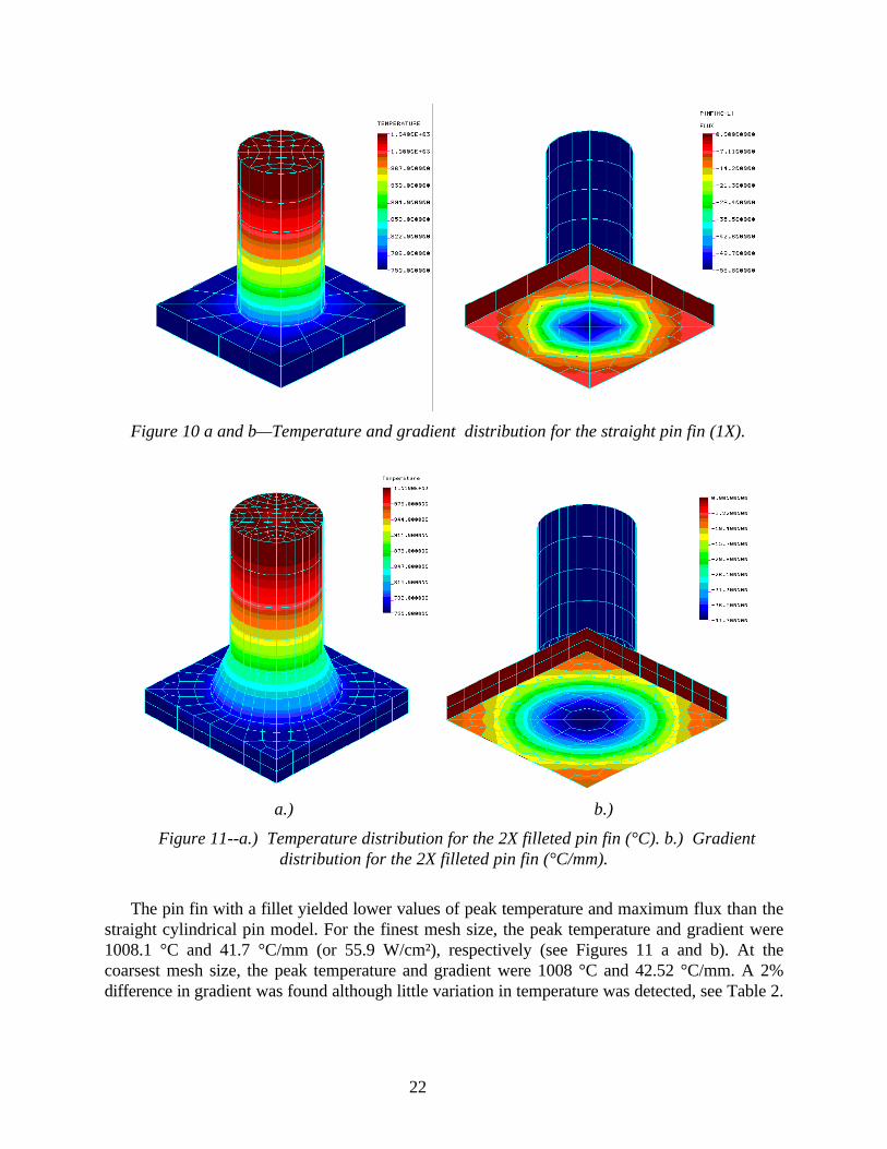
Figure 10 a and b—Temperature and gradient distribution for the straight pin fin (1X).

a.) b.)

Figure 11--a.) Temperature distribution for the 2X filleted pin fin (°C). b.) Gradientdistribution for the 2X filleted pin fin (°C/mm).

The pin fin with a fillet yielded lower values of peak temperature and maximum flux than thestraight cylindrical pin model. For the finest mesh size, the peak temperature and gradient were1008.1 °C and 41.7 °C/mm (or 55.9 W/cm²), respectively (see Figures 11 a and b). At thecoarsest mesh size, the peak temperature and gradient were 1008 °C and 42.52 °C/mm. A 2%difference in gradient was found although little variation in temperature was detected, see Table 2.

23

In Figure 11 b, note the non-circular shape of the gradient distribution on the bottom surfacemainly at the periphery. While a non-circular pattern over the entire plate surface is moreapparent in the straight pin image of Figure 10, the latter was based on a coarser mesh.Interpolation of values between nodes is being performed by the visualization package and leadsto the apparently non-circular pattern at the central region. With more nodes, the linearity wouldchange over towards a more circular appearance. Thus, the output from visualization shouldalways be interpreted with due respect given to the characteristic geometry of the mesh used.

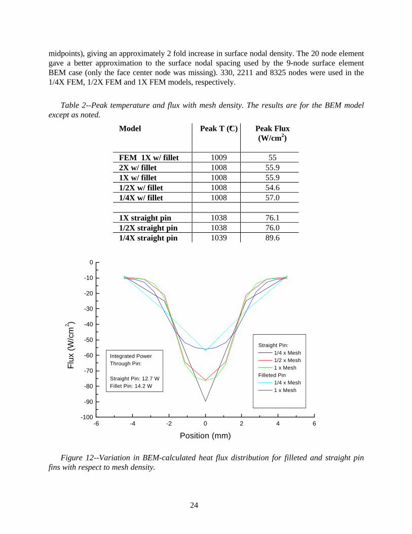
Figure 12 shows the flux profile along the diagonal of the bottom surface. As can be seen,the filleted pin has very similar values for the peak flux regardless of mesh size, while the lowdensity mesh of the straight pin has a peak flux value much different than those at the higher meshsizes. The low-density meshes for the filleted and straight pins have only four nodal points alongthis diagonal. It appears to be fortuitous that the peak flux value from the low-density mesh of thefilleted pin matches that of the higher density meshes. The solution is similar because thetriangular shape of the low-density curve had offsetting negative and positive errors and bettersimulated the well-balanced bell shape of the higher density mesh cases. Thus, the lowest densityor coarsest mesh (1/4X) appears too coarse for reliable results. Even though the exact solution isunknown it appears that with mesh refinement, the numerical solution is convergent to aconsistent value.

The reduction in peak temperature and flux with the filleted pin fin design is the desiredoutcome of the pin fin models. The application of interest requires peak temperatures and fluxesto be as low as possible. The filleted pin fin better provides this combination of properties ascompared to the straight pin fin. Material degradation at high temperatures results in decreasedlifetime of the unit due to pin erosion by the aggressive flue gas, and higher fluxes lead to greaterevaporation rates than the capillary pumping capability of the wick (which provides the sodiumreplacement). Lower flux reduces the rate of evaporation of sodium off of the bottom surface.Also, sodium evaporation is providing the constant temperature boundary condition at 750 °C.The filleted pin fin model is a better representation of the actual pin fin geometry. The modelresults show that the fillet does indeed significantly improve pin performance over the idealizedpin originally modeled.

The addition of the fillet to the model decreased the peak temperature by about 3% andthe peak flux by about 25%. The power throughput of the pin increased about 12%. This isprimarily the result of a larger cross-sectional heat transfer area. In addition, the lower pintemperature results in a higher thermal driving potential from the free stream, again resulting inincreased throughput.

Pin Fin FEM Results

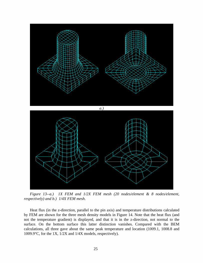
A series of varying mesh density FEM calculations were made for the filleted pin fin. Thesewere run on a Macintosh PowerPC. The surface-appearance of the meshes used were similar butnot identical to those used for the BEM calculations. Figure 13 shows the meshes used. In thefirst two cases, 8 node solid elements were used (a node at each corner), while for the last casethe same mesh was used but 20 node solid elements were used instead (nodes at corners and edge

24

midpoints), giving an approximately 2 fold increase in surface nodal density. The 20 node elementgave a better approximation to the surface nodal spacing used by the 9-node surface elementBEM case (only the face center node was missing). 330, 2211 and 8325 nodes were used in the1/4X FEM, 1/2X FEM and 1X FEM models, respectively.

Table 2--Peak temperature and flux with mesh density. The results are for the BEM modelexcept as noted.

Model Peak T (°C) Peak Flux(W/cm2)

FEM 1X w/ fillet 1009 552X w/ fillet 1008 55.91X w/ fillet 1008 55.91/2X w/ fillet 1008 54.61/4X w/ fillet 1008 57.0

1X straight pin 1038 76.11/2X straight pin 1038 76.01/4X straight pin 1039 89.6

-6 -4 -2 0 2 4 6-100

-90

-80

-70

-60

-50

-40

-30

-20

-10

0

Integrated PowerThrough Pin:

Straight Pin: 12.7 WFillet Pin: 14.2 W

Straight Pin: 1/4 x Mesh 1/2 x Mesh 1 x Mesh

Filleted Pin 1/4 x Mesh 1 x Mesh

Flu

x (W

/cm

2 )

Position (mm)

Figure 12--Variation in BEM-calculated heat flux distribution for filleted and straight pinfins with respect to mesh density.

25

a.)

Figure 13--a.) 1X FEM and 1/2X FEM mesh (20 nodes/element & 8 nodes/element,respectively) and b.) 1/4X FEM mesh.

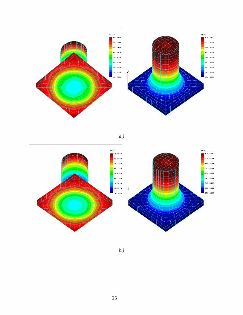
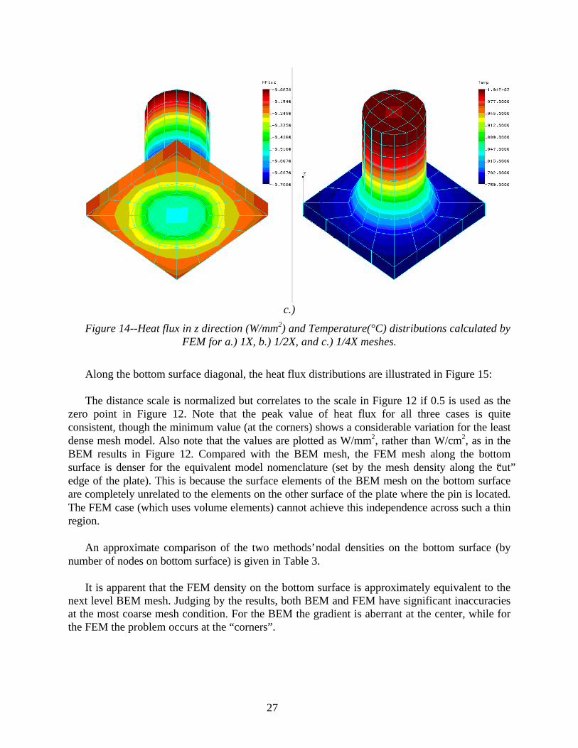
Heat flux (in the z-direction, parallel to the pin axis) and temperature distributions calculatedby FEM are shown for the three mesh density models in Figure 14. Note that the heat flux (andnot the temperature gradient) is displayed, and that it is in the z-direction, not normal to thesurface. On the bottom surface this latter distinction vanishes. Compared with the BEMcalculations, all three gave about the same peak temperature and location (1009.1, 1008.8 and1009.9°C, for the 1X, 1/2X and 1/4X models, respectively).

26

a.)

b.)

27

c.)

Figure 14--Heat flux in z direction (W/mm2) and Temperature(°C) distributions calculated byFEM for a.) 1X, b.) 1/2X, and c.) 1/4X meshes.

Along the bottom surface diagonal, the heat flux distributions are illustrated in Figure 15:

The distance scale is normalized but correlates to the scale in Figure 12 if 0.5 is used as thezero point in Figure 12. Note that the peak value of heat flux for all three cases is quiteconsistent, though the minimum value (at the corners) shows a considerable variation for the leastdense mesh model. Also note that the values are plotted as W/mm2, rather than W/cm2, as in theBEM results in Figure 12. Compared with the BEM mesh, the FEM mesh along the bottomsurface is denser for the equivalent model nomenclature (set by the mesh density along the “cut”edge of the plate). This is because the surface elements of the BEM mesh on the bottom surfaceare completely unrelated to the elements on the other surface of the plate where the pin is located.The FEM case (which uses volume elements) cannot achieve this independence across such a thinregion.

An approximate comparison of the two methods’ nodal densities on the bottom surface (bynumber of nodes on bottom surface) is given in Table 3.

It is apparent that the FEM density on the bottom surface is approximately equivalent to thenext level BEM mesh. Judging by the results, both BEM and FEM have significant inaccuraciesat the most coarse mesh condition. For the BEM the gradient is aberrant at the center, while forthe FEM the problem occurs at the “corners”.

28

Figure 15--Heat flux in z direction (W/mm2) along bottom diagonal of pin fin, calculated byFEM for 1X, 1/2X, and 1/4X meshes.

Table 3--Comparison of BEM and TEM bottom surface nodal density (number of bottomsurface nodes in models)

BEM FEM2X 577 -1X 177 6651/2X 57 2411/4X 25 57

Timing Results

Without an optimization level for the compiler specified, BEM calculation times as long as272 seconds were obtained for the pin fin with fillet, (1x mesh) on the RS6000 computer. Tofurther improve the times, optimizer levels of 2 and 3 (xlF compiler) were used for compiling theexecutable program. It was seen that an order of magnitude decrease in timing could be obtainedwith a good optimizer on the BEM code. The results are summarized in Table 4.

Figure 16 a-c contains the timing results from three cube files, 3 pin fin without fillet files, and4 pin fin with fillet files. The number of nodes vs the time (in seconds) is shown in Table 5 for allof the files. The linear curve fit of the log MATVEC time vs log nodes yielded a slope of 1.65; logDECOMP/SOLVE vs log nodes yielded a slope of 2.92; and, log total time vs log nodes yielded aslope of 2.03.

29

Table 4--Comparison of BEM run times with differing levels of code optimization on theRS6000 computer.

Optimizerlevel

GEOMtime(seconds)

MATVECtime(seconds)

LU/SOLVEtime(seconds)

Outputtime(seconds)

Total time(seconds)

not specified 0.18 114 160 0.06 27202 0.2 36 21 0.05 5803 0.2 33 21 0.06 54

The MATVEC subroutine uses a do loop on nodes with a call to subroutine INT4, which usesa do loop around the number of local nodes, and then performs another do loop on nodes in themain subroutine followed by another do loop on nodes. Thus, subroutine MATVEC should beorder 2 (O2). The time to collect and assemble the matrices—A, B, phi, phip, etc.—is dominating theprocesses for the matrix sizes used in this experiment, since the overall order is about 2. Withlarger matrices, the LU Decomposition subroutine should eventually dominate the program andyield order three, as seen by the value of 2.92 for the slope of the log DECOMP/SOLVE vs lognodes plot. This reflects the relatively short triple do loop around the number of nodes in the LUDECOMP subroutine. Note that the SOLVE subroutine has two do loops on the number ofnodes, therefore the LU Decomposition subroutine dominates the process. The memory storageprocess is order 2. It appears that the constant multiplier for the order 2 processes in the codedominate the smaller multiplier for time contribution from DECOMP/SOLVE, which is order 3.With larger arrays/matrix, it is expected that the overall performance should scale as order 3.

Table 5--Output from timing tests for differing number of nodes. Results were obtained usingan IBM RS6000 with an optimizer level of 2 and requesting uninterrupted use of one processor.

Model Nodes GEOMtime(seconds)

MATVECtime(seconds)

DECOMP/SOLVEtime(seconds)

Outputtime(seconds)

Total time(seconds)

4 el/side Cube 150 0.03 1.43 0.1 0.01 1.571/4X Straight 322 0.08 6.87 0.89 0.02 7.86

1/4X Fillet 322 0.07 6.69 0.89 0.01 7.661/2X Straight 354 0.08 8.41 1.1 0.01 9.6

1/2X Fillet 354 0.07 8.33 1.1 0.02 9.5216 el/side Cube 486 0.07 9.82 2.91 0.02 12.82

1X Fillet 962 0.19 36.32 21.04 0.05 57.61X Straight 971 0.18 37.28 21.59 0.05 59.1

64 el/side Cube 1734 0.3 89.2 125.8 0.09 215.32X Fillet 2562 0.53 206 394.5 0.13 601.9

30

5.0 5.5 6.0 6.5 7.0 7.5 8.0

0

1

2

3

4

5

6

7

LU Decomp/Solveslope = 2.92

Total Timeslope = 2.03

MatVecslope = 1.65

log

tota

l tim

e

log nodes

Figure 16—BEM Timing results for total time and portions of the code. Time is in seconds.

The finite element code, COSMOS/M, was used on the filleted pin fin as a comparison ofresults from the BEM code. The resulting times were 51 seconds total time for the FEM codeusing a highly optimized COSMOS/M proprietary code and an 8871-node model, 306 secondstotal time for an older, non-proprietary COSMOS/M code, and 1420 seconds for the 2X pin fin(2562 nodes) BEM model on the PC. The FEM model in this case had a greater surface density ofelements than the BEM model. However, the FEM model uses highly optimized code, while theFORTRAN compiler (Microsoft Powerstation FORTRAN) has limited optimization. Note thatthe BEM times are much slower on the PC than on the RS6000, while the computational speed ofthe machines are similar. These timings were performed on a Pentium 90 with 80 M of RAM.COSMOS/M is not available on the RS6000.

Further timing measurements for the less complex FEM models run on the Macintosh PowerPC (with 40 M of RAM and a 100 Mhz processor) gave values of 1231 seconds total time for the1X FEM model (8325 nodes), 138 seconds for the 1/2X model (2211 nodes) and 19 seconds forthe 1/4X model (330 nodes). These times are considerably slower than the times on the PC. Mostof the total time was spent assembling and decomposing the matrices; actual solution time tookonly about 5-7% of the total time. Plotting total time values on a log-log plot (Figure 17), theslope is found to be 1.27, which is of considerably lower order than the BEM code.

The computation time increase caused by model complexity is of order 1.27 for the FEM and2 for the BEM. However, as the mesh density increases, the number of nodes in the FEM modelincreases as N³ where N is the number of nodes in a given linear direction, while the nodes on a

31

BEM model increase as N². Thus, the actual order of time increase with linear node density is 3.8for FEM and 4.1 for the BEM method. Given all the variables involved, these orders are verysimilar. A more exhaustive study using good optimization on the same machine would beappropriate. In addition, the accuracy of the solution would be a better comparison than surfacenodal density.

1

1.5

2

2.5

3

3.5

2.5 3 3.5 4

Lo

g t

ota

l cal

c ti

me

Log nodes

curve fit

slope = 1.27

Figure 17--Total FEM calculation time vs number of nodes in model.

Summary/Conclusions

It was determined that the weld fillet on the pin fin significantly enhanced the heat transfer tothe sodium working fluid, improving the operating margin of the heat pipe. The peak flux wasreduced by 25% under the worst-case scenario, while the peak pin temperature was slightlyreduced, when compared to the previously modeled idealized pin fin. The reduced pintemperature and fixed gas temperature resulted in 12% more total power that could be transferredby the pin. These significant changes in pin performance should be incorporated into the overallheat-pipe performance models, including the Fluent CFD model and the heat pipe wick model.

32

In the models investigated, there is not a clear advantage in computational time for either theBEM or FEM methods, though the proprietary optimized COSMOS/M FEM code on a PentiumPC appears to be the fastest method investigated. Processor speeds and code optimizationcapabilities differed between the machines used. A more careful study should be performed withgeometries that have analytical solutions and with good optimizing compilers.

In the range of model sizes investigated, the BEM and FEM codes have similar scalabilitybased on linear grid spacing. However, the BEM code has a higher order (O(3) based on numberof nodes) routine (LU Solve) that will dominate on very large models, and thus may be lessscaleable than the FEM method.

A process for performing 3-dimensional BEM analysis was developed, tested, and applied tothe problem at hand. The process is as follows:

i.) Model the part and perform mesh generation over the surface. (Use of the COSMOS/Mprogram was helpful for this task, however other packages that would provide the same resultsare available. It is necessary to assure that surface normals are oriented properly.

ii.) Supply information from mesh generation to the mesh converter program in order to forman input file with the necessary format for the BEM program.

iii.) Run Marc Ingber’s BEM program (NPOT3D) with the input file and obtain an output fileof node number and temperature and flux for every node.

iv.) Graph the output file. In our work this was supplied to COSMOS/M as a user definedplotfile to obtain 3-dimensional graphing of the temperature or flux over the object surface.Limitations of the graphics output must be considered in the interpretation of data (i.e. polygonalplotting of cylindrical elements, linear interpolation of data between nodes).

v.) Additionally, information such as peak temperatures and flux can be obtained directly fromsimple sorting or statistical analysis of the data in the output file.

vi.) The BEM solutions at points inside the object can be obtained by supplying thecoordinates of interest into the input file. The severity number indicates accuracy of the result. Ifno severity number is reported, the accuracy is good.

In summary, an existing FEM mesh-generation tool was used to develop complex meshes forthe BEM technique in conjunction with an automated conversion routine that incorporatedboundary conditions and some error checking.

Acknowledgments

The authors thank Marc Ingber, Scott Rawlinson, Brian Smith, and Richard Allen for theirhelp and encouragement with this work. This work was performed at the University of NewMexico, Albuquerque Resource Center, and Sandia National Laboratories, which is operated forthe U.S. Department of Energy under contract number DE-AC04-94AL85000.

33

References

1 Fluent UNS, West Lebanon, NH.2 COSMOS/M, Structural Research and Analysis Corporation, Los Angeles, CA.3 Marc S. Ingber, npot3d.f BEM code.4 Diver, R.B., et al, “Trends in Dish Stirling Solar Receiver Design,” paper no. 905303,

Proceedings of the 25th IECEC, Reno NV, August, 1990.5 Marc S. Ingber, SAND93-7072, Sandia National Laboratories report, Albuquerque, NM

(1993).6 Marc S. Ingber memo to D. W. Larson, Sandia National Laboratories, Albuquerque, NM

(August 10, 1987).7 High Performance Computing, Schauble et al. (1990).8 Matlab, The MathWorks Inc., Natick, MA.9 Mathematica, Wolfram Research Inc., Champaign, IL.

34

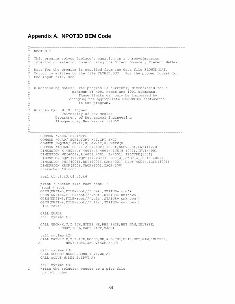
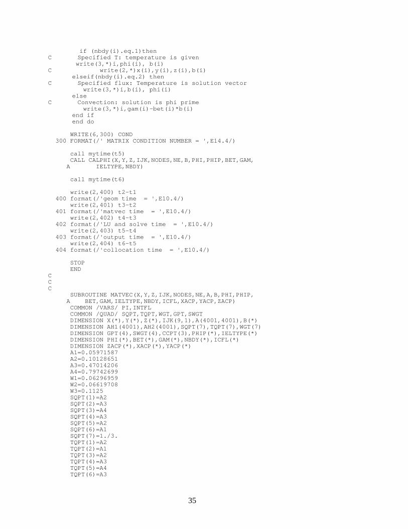
Appendix A. NPOT3D BEM Code

C=========================================================================C NPOT3d.fCC This program solves Laplace's equation in a three-dimensionC interior or exterior domain using the Direct Boundary Element Method.CC Data for the program is supplied from the data file FLOW3D.DAT.C Output is written to the file FLOW3D.OUT. For the proper format forC the input file, seeCCC Dimensioning Notes: The program is currently dimensioned for aC maximum of 4001 nodes and 1001 elements.C These limits can only be increased byC changing the appropriate DIMENSION statementsC in the program.CC Written by: M. S. IngberC University of New MexicoC Department of Mechanical EngineeringC Albuquerque, New Mexico 87185*CCC======================================================================== COMMON /VARS/ PI,INTFL COMMON /QUAD/ SQPT,TQPT,WGT,GPT,SWGT COMMON /NQUAD/ GP(12,8),GW(12,8),NSEV(8) COMMON /TQUAD/ SGP(112,8),TGP(112,8),NSEV2(8),GWT(112,8) DIMENSION X(4001),Y(4001),Z(4001),IJK(9,1001),IPVT(4001) DIMENSION WK(4001),A(4001,4001),B(4001),IELTYPE(1001) DIMENSION SQPT(7),TQPT(7),WGT(7),GPT(4),SWGT(4),PHIP(4001) DIMENSION PHI(4001),BET(4001),GAM(4001),NBDY(4001),ICFL(4001) DIMENSION XACP(200),YACP(200),ZACP(200) character *8 root

real t1,t2,t3,t4,t5,t6

print *,'Enter file root name: 'read *,root

OPEN(UNIT=5,FILE=root//'.dek',STATUS='old') OPEN(UNIT=6,FILE=root//'.out',STATUS='unknown') OPEN(UNIT=3,FILE=root//'.plt',STATUS='unknown') OPEN(UNIT=2,FILE=root//'.flx',STATUS='unknown') PI=4.*ATAN(1.)

CALL QUADR call mytime(t1)

CALL GEOM(X,Y,Z,IJK,NODES,NE,PHI,PHIP,BET,GAM,IELTYPE, A NBDY,ICFL,XACP,YACP,ZACP)

call mytime(t2) CALL MATVEC(X,Y,Z,IJK,NODES,NE,A,B,PHI,PHIP,BET,GAM,IELTYPE, A NBDY,ICFL,XACP,YACP,ZACP)

call mytime(t3) CALL DECOMP(NODES,COND,IPVT,WK,A) CALL SOLVE(NODES,B,IPVT,A)

call mytime(t4)C Write the solution vector to a plot file

do i=1,nodes

35

if (nbdy(i).eq.1)thenC Specified T: temperature is given write(3,*)i,phi(i), b(i)C write(2,*)x(i),y(i),z(i),b(i)

elseif(nbdy(i).eq.2) thenC Specified flux: Temperature is solution vector

write(3,*)i,b(i), phi(i)else

C Convection: solution is phi prime write(3,*)i,gam(i)-bet(i)*b(i)end ifend do

WRITE(6,300) COND 300 FORMAT(/' MATRIX CONDITION NUMBER = ',E14.4/)

call mytime(t5) CALL CALPHI(X,Y,Z,IJK,NODES,NE,B,PHI,PHIP,BET,GAM, A IELTYPE,NBDY)

call mytime(t6)

write(2,400) t2-t1 400 format(/'geom time = ',E10.4/) write(2,401) t3-t2 401 format(/'matvec time = ',E10.4/) write(2,402) t4-t3 402 format(/'LU and solve time = ',E10.4/) write(2,403) t5-t4 403 format(/'output time = ',E10.4/) write(2,404) t6-t5 404 format(/'collocation time = ',E10.4/)

STOP ENDCCC SUBROUTINE MATVEC(X,Y,Z,IJK,NODES,NE,A,B,PHI,PHIP, A BET,GAM,IELTYPE,NBDY,ICFL,XACP,YACP,ZACP) COMMON /VARS/ PI,INTFL COMMON /QUAD/ SQPT,TQPT,WGT,GPT,SWGT DIMENSION X(*),Y(*),Z(*),IJK(9,1),A(4001,4001),B(*) DIMENSION AH1(4001),AH2(4001),SQPT(7),TQPT(7),WGT(7) DIMENSION GPT(4),SWGT(4),CCPT(3),PHIP(*),IELTYPE(*) DIMENSION PHI(*),BET(*),GAM(*),NBDY(*),ICFL(*) DIMENSION ZACP(*),XACP(*),YACP(*) A1=0.05971587 A2=0.10128651 A3=0.47014206 A4=0.79742699 W1=0.06296959 W2=0.06619708 W3=0.1125 SQPT(1)=A2 SQPT(2)=A3 SQPT(3)=A4 SQPT(4)=A3 SQPT(5)=A2 SQPT(6)=A1 SQPT(7)=1./3. TQPT(1)=A2 TQPT(2)=A1 TQPT(3)=A2 TQPT(4)=A3 TQPT(5)=A4 TQPT(6)=A3

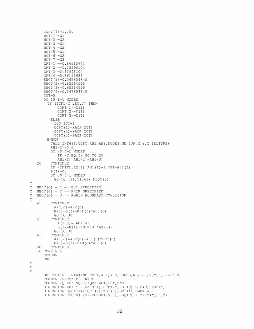
36

TQPT(7)=1./3. WGT(1)=W1 WGT(2)=W2 WGT(3)=W1 WGT(4)=W2 WGT(5)=W1 WGT(6)=W2 WGT(7)=W3 GPT(1)=-0.86113631 GPT(2)=-0.33998104 GPT(3)=0.33998104 GPT(4)=0.86113631 SWGT(1)=0.347854845 SWGT(2)=0.65214515 SWGT(3)=0.65214515 SWGT(4)=0.347854845 ICT=0 DO 10 I=1,NODES IF (ICFL(I).EQ.0) THEN CCPT(1)=X(I) CCPT(2)=Y(I) CCPT(3)=Z(I) ELSE

ICT=ICT+1 CCPT(1)=XACP(ICT) CCPT(2)=YACP(ICT) CCPT(3)=ZACP(ICT)

ENDIF CALL INT4(I,CCPT,AH1,AH2,NODES,NE,IJK,X,Y,Z,IELTYPE) AH1(I)=0.0 DO 20 J=1,NODES IF (J.EQ.I) GO TO 20 AH1(I)=AH1(I)-AH1(J) 20 CONTINUE IF (INTFL.EQ.1) AH1(I)=4.*PI+AH1(I) B(I)=0. DO 30 J=1,NODES

GO TO (41,51,61) NBDY(J)CC NBDY(J) = 1 => PHI SPECIFIEDC NBDY(J) = 2 => PHIP SPECIFIEDC NBDY(J) = 3 => ROBIN BOUNDARY CONDITIONC 41 CONTINUE

A(I,J)=AH2(J) B(I)=B(I)+PHI(J)*AH1(J) GO TO 30

51 CONTINUE A(I,J)=-AH1(J) B(I)=B(I)-PHIP(J)*AH2(J)

GO TO 30 61 CONTINUE

A(I,J)=AH2(J)+AH1(J)*BET(J) B(I)=B(I)+GAM(J)*AH1(J)

30 CONTINUE 10 CONTINUE RETURN ENDCCC SUBROUTINE INT4(INO,CCPT,AH1,AH2,NODES,NE,IJK,X,Y,Z,IELTYPE) COMMON /VARS/ PI,INTFL COMMON /QUAD/ SQPT,TQPT,WGT,GPT,SWGT DIMENSION AH1(*),IJK(9,1),CCPT(*),G1(9),G1P(9),AH2(*) DIMENSION SQPT(7),TQPT(7),WGT(7),GPT(4),SWGT(4) DIMENSION COORD(3,9),COORDT(9,3),DSQ(9),X(*),Y(*),Z(*)

37

DIMENSION IELTYPE(*) SMALL=1.E-6 DO 5 I=1,NODES AH1(I)=0.0 AH2(I)=0.0 5 CONTINUE DO 10 I=1,NE IF (IELTYPE(I).LT.40) THEN

NS=6 COORD(1,1)=X(IJK(1,I)) COORD(2,1)=Y(IJK(1,I)) COORD(3,1)=Z(IJK(1,I)) COORD(1,2)=X(IJK(2,I)) COORD(2,2)=Y(IJK(2,I)) COORD(3,2)=Z(IJK(2,I)) COORD(1,3)=X(IJK(3,I)) COORD(2,3)=Y(IJK(3,I)) COORD(3,3)=Z(IJK(3,I)) COORD(1,4)=X(IJK(4,I)) COORD(2,4)=Y(IJK(4,I)) COORD(3,4)=Z(IJK(4,I)) COORD(1,5)=X(IJK(5,I)) COORD(2,5)=Y(IJK(5,I)) COORD(3,5)=Z(IJK(5,I)) COORD(1,6)=X(IJK(6,I)) COORD(2,6)=Y(IJK(6,I)) COORD(3,6)=Z(IJK(6,I)) DO 15 IC=1,3 DO 15 JC=1,6 COORDT(JC,IC)=COORD(IC,JC) 15 CONTINUE DO 25 IC=1,6 DSQ(IC)=(COORD(1,IC)-CCPT(1))**2+(COORD(2,IC)- A CCPT(2))**2+(COORD(3,IC)-CCPT(3))**2 DSQ(IC)=SQRT(DSQ(IC)) 25 CONTINUE INODE=0 IF (DSQ(1).LE.SMALL) INODE=1 IF (DSQ(2).LE.SMALL) INODE=2 IF (DSQ(3).LE.SMALL) INODE=3 IF (DSQ(4).LE.SMALL) INODE=4 IF (DSQ(5).LE.SMALL) INODE=5 IF (DSQ(6).LE.SMALL) INODE=6 IF (INODE.EQ.0) THEN CALL RTINT(CCPT,G1,G1P,COORD,COORDT) ELSE CALL STINT(CCPT,G1,G1P,COORD,COORDT,INODE) END IF ELSE

NS=9 COORD(1,1)=X(IJK(1,I)) COORD(2,1)=Y(IJK(1,I)) COORD(3,1)=Z(IJK(1,I)) COORD(1,2)=X(IJK(2,I)) COORD(2,2)=Y(IJK(2,I)) COORD(3,2)=Z(IJK(2,I)) COORD(1,3)=X(IJK(3,I)) COORD(2,3)=Y(IJK(3,I)) COORD(3,3)=Z(IJK(3,I)) COORD(1,4)=X(IJK(4,I)) COORD(2,4)=Y(IJK(4,I)) COORD(3,4)=Z(IJK(4,I)) COORD(1,5)=X(IJK(5,I)) COORD(2,5)=Y(IJK(5,I)) COORD(3,5)=Z(IJK(5,I)) COORD(1,6)=X(IJK(6,I)) COORD(2,6)=Y(IJK(6,I))

38

COORD(3,6)=Z(IJK(6,I)) COORD(1,7)=X(IJK(7,I)) COORD(2,7)=Y(IJK(7,I))

COORD(3,7)=Z(IJK(7,I)) COORD(1,8)=X(IJK(8,I))

COORD(2,8)=Y(IJK(8,I)) COORD(3,8)=Z(IJK(8,I))

COORD(1,9)=X(IJK(9,I)) COORD(2,9)=Y(IJK(9,I)) COORD(3,9)=Z(IJK(9,I))

DO 16 IC=1,3 DO 16 JC=1,9 COORDT(JC,IC)=COORD(IC,JC) 16 CONTINUE DO 26 IC=1,9 DSQ(IC)=(COORD(1,IC)-CCPT(1))**2+(COORD(2,IC)- A CCPT(2))**2+(COORD(3,IC)-CCPT(3))**2 DSQ(IC)=SQRT(DSQ(IC)) 26 CONTINUE INODE=0 IF (DSQ(1).LE.SMALL) INODE=1 IF (DSQ(2).LE.SMALL) INODE=2 IF (DSQ(3).LE.SMALL) INODE=3 IF (DSQ(4).LE.SMALL) INODE=4 IF (DSQ(5).LE.SMALL) INODE=5 IF (DSQ(6).LE.SMALL) INODE=6 IF (DSQ(7).LE.SMALL) INODE=7 IF (DSQ(8).LE.SMALL) INODE=8

IF (DSQ(9).LE.SMALL) INODE=9 IF (INODE.EQ.0) THEN CALL RQINT(CCPT,G1,G1P,COORD,COORDT,IELTYPE(I)) ELSE CALL SQINT(CCPT,G1,G1P,COORD,COORDT,INODE,IELTYPE(I)) END IF END IF DO 20 J=1,NS AH1(IJK(J,I))=AH1(IJK(J,I))+G1P(J) AH2(IJK(J,I))=AH2(IJK(J,I))+G1(J) 20 CONTINUE 10 CONTINUE RETURN ENDCCC SUBROUTINE RTINT(CCPT,G1,G1P,COORD,COORDT) COMMON /VARS/ PI,INTFL COMMON /QUAD/ SQPT,TQPT,WGT,GPT,SWGT COMMON /TQUAD/ SGP(112,8),TGP(112,8),NSEV2(8),GWT(112,8) DIMENSION CCPT(*),G1(*),G1P(*),COORD(3,9),COORDT(9,3) DIMENSION SQPT(7),TQPT(7),WGT(7),GPT(4),SWGT(4) DIMENSION DLH(2,6),DGH(2,3),RJ(2,2),QNORM(3) DIMENSION UNORM(3),F(9),FP(9),CEN(3),DVEC(3) DO 5 I=1,6 G1(I)=0. G1P(I)=0. 5 CONTINUECC DETERMINE SEVERITYCC FIND LONGEST SIDE OF TRIANGLEC S1=SQRT((COORD(1,2)-COORD(1,1))**2+(COORD(2,2)- A COORD(2,1))**2+(COORD(3,2)-COORD(3,1))**2) H=S1 S2=SQRT((COORD(1,3)-COORD(1,2))**2+(COORD(2,3)- A COORD(2,2))**2+(COORD(3,3)-COORD(3,2))**2)

39

IF (S2.GT.H) H=S2 S3=SQRT((COORD(1,1)-COORD(1,3))**2+(COORD(2,1)- A COORD(2,3))**2+(COORD(3,1)-COORD(3,3))**2) IF (S3.GT.H) H=S3 DO 59 I=1,3

A1=COORD(I,1)+COORD(I,2)+COORD(I,3) A2=COORD(I,4)+COORD(I,5)+COORD(I,6)

CEN(I)=4.*A2/9.-A1/9. 59 CONTINUE DVEC(1)=CCPT(1)-CEN(1) DVEC(2)=CCPT(2)-CEN(2) DVEC(3)=CCPT(3)-CEN(3) D=SQRT(DVEC(1)**2+DVEC(2)**2+DVEC(3)**2) HDD=H/D IF (HDD.LT.0.358) THEN

ISEV=1 ELSE

CALL DER6T(1./3.,1./3.,DLH) DO 16 IC=1,2 DO 16 JC=1,3 SUM=0.0

DO 36 KC=1,6 SUM=SUM+DLH(IC,KC)*COORDT(KC,JC)

36 CONTINUE DGH(IC,JC)=SUM

16 CONTINUE QNORM(1)=DGH(1,2)*DGH(2,3)-DGH(1,3)*DGH(2,2) QNORM(2)=DGH(1,3)*DGH(2,1)-DGH(1,1)*DGH(2,3)

QNORM(3)=DGH(1,1)*DGH(2,2)-DGH(1,2)*DGH(2,1) CALL UNORMAL(QNORM,UNORM) UDOTD=0.0 DO 41 I=1,3 UDOTD=UDOTD+UNORM(I)*DVEC(I)

41 CONTINUE COSTH=ABS(UDOTD/D) ISEV=(2.37+0.424*COSTH)*HDD+1 IF (ISEV.GE.9) THEN WRITE(6,100) ISEV,(CCPT(I),I=1,3) ISEV=8 ENDIF

ENDIF 100 FORMAT(/' WARNING, SEVERITY NUMBER=',I2,' AT CCPT= (', A E10.4,',',E10.4,',',E10.4,')'/' LARGE QUADRATURE B ERRORS ARE POSSIBLE'/) NQ=NSEV2(ISEV) DO 60 I=1,NQ CALL DER6T(SGP(I,ISEV),TGP(I,ISEV),DLH) DO 15 IC=1,2 DO 25 JC=1,3 SUM=0. DO 35 KC=1,6 SUM=SUM+DLH(IC,KC)*COORDT(KC,JC) 35 CONTINUE DGH(IC,JC)=SUM 25 CONTINUE 15 CONTINUE DO 50 IC=1,2 DO 40 JC=1,2 SUM=0. DO 30 KC=1,3 SUM=SUM+DGH(IC,KC)*DGH(JC,KC) 30 CONTINUE RJ(IC,JC)=SUM 40 CONTINUE 50 CONTINUE DET2=RJ(1,1)*RJ(2,2)-RJ(1,2)*RJ(2,1) DETWT=SQRT(DET2)*GWT(I,ISEV)

40

QNORM(1)=DGH(1,2)*DGH(2,3)-DGH(1,3)*DGH(2,2) QNORM(2)=DGH(1,3)*DGH(2,1)-DGH(1,1)*DGH(2,3) QNORM(3)=DGH(1,1)*DGH(2,2)-DGH(1,2)*DGH(2,1) CALL UNORMAL(QNORM,UNORM) CALL FUNDS(SGP(I,ISEV),TGP(I,ISEV),COORD,CCPT,UNORM,F,FP,30) DO 10 J=1,6 G1(J)=G1(J)+F(J)*DETWT G1P(J)=G1P(J)+FP(J)*DETWT 10 CONTINUE 60 CONTINUE RETURN ENDCCC SUBROUTINE FUNDS(S,T,COORD,CCPT,UNORM,F,FP,IET) DIMENSION COORD(3,9),CCPT(*),UNORM(*),H(9),F(9),FP(9) DIMENSION QPT(3) IF (IET.LT.40) THEN NS=6C IF (IET.EQ.30) THEN CALL SHP6T(S,T,H)C ELSEC CALL SHP6TD(S,T,H)C ENDIF ELSE

NS=9 IF (IET.EQ.40) THEN

CALL SHP9T(S,T,H) ELSE

CALL SHP9TD(S,T,H) ENDIF

ENDIF DO 10 I=1,3 QPT(I)=0. DO 10 J=1,NS QPT(I)=COORD(I,J)*H(J)+QPT(I) 10 CONTINUE R=SQRT((CCPT(1)-QPT(1))**2+(CCPT(2)-QPT(2))**2+(CCPT(3)- A QPT(3))**2) F1=(CCPT(1)-QPT(1))*UNORM(1)/R**3 F2=(CCPT(2)-QPT(2))*UNORM(2)/R**3 F3=(CCPT(3)-QPT(3))*UNORM(3)/R**3 DO 20 I=1,NS FP(I)=(F1+F2+F3)*H(I) F(I)=H(I)/R 20 CONTINUE RETURN ENDCCC SUBROUTINE DER6T(S,T,DLH) DIMENSION DLH(2,6) DLH(1,1)=2.*(S+T-0.5)+2.*(S+T-1.) DLH(1,2)=2.*(S-0.5)+2.*S DLH(1,3)=0. DLH(1,4)=-4.*(S+T-1.)-4.*S DLH(1,5)=4.*T DLH(1,6)=-4.*T DLH(2,1)=DLH(1,1) DLH(2,2)=0. DLH(2,3)=2.*(T-0.5)+2.*T DLH(2,4)=-4.*S DLH(2,5)=4.*S DLH(2,6)=-4.*(S+T-1.)-4.*T RETURN

41

ENDCCC SUBROUTINE UNORMAL(Q,U) COMMON /VARS/ PI,INTFL DIMENSION Q(*),U(*) F=1. IF (INTFL.EQ.1) F=-1. R=SQRT(Q(1)**2+Q(2)**2+Q(3)**2) U(1)=F*Q(1)/R U(2)=F*Q(2)/R U(3)=F*Q(3)/R RETURN ENDCCC SUBROUTINE SHP6T(S,T,H) DIMENSION H(9) H(1)=2.*(S+T-0.5)*(S+T-1.) H(2)=2.*S*(S-0.5) H(3)=2.*T*(T-0.5) H(4)=-4.*S*(S+T-1.) H(5)=4.*S*T H(6)=-4.*T*(S+T-1.) RETURN ENDCCC SUBROUTINE STINT(CCPT,G1,G1P,COORD,COORDT,INODE) COMMON /VARS/ PI,INTFL COMMON /QUAD/ SQPT,TQPT,WGT,GPT,SWGT DIMENSION CCPT(*),G1(*),G1P(*),COORD(3,9),COORDT(9,3) DIMENSION SQPT(7),TQPT(7),WGT(7),GPT(4),SWGT(4) DIMENSION NODE(6),DLH(2,6),DGH(2,3),RJ(2,2) DIMENSION NORDER(6,6),UNORM(3),QNORM(3),QPT(3) DIMENSION F(9),FP(9),G1H(9),G1PH(9) DATA NORDER/1,2,3,3,1,2,2,3,1,1,2,3,3,1,2,2,3,1,4,5,6 A ,6,4,5,5,6,4,4,5,6,6,4,5,5,6,4/ DO 10 I=1,6 NODE(I)=NORDER(INODE,I) 10 CONTINUE DO 20 J=1,6 NOD=NODE(J) DO 30 I=1,3 COORDT(J,I)=COORD(I,NOD) 30 CONTINUE 20 CONTINUE DO 40 I=1,3 DO 40 J=1,6 COORD(I,J)=COORDT(J,I) 40 CONTINUE IF (INODE.LE.3) THEN INDX=1 FACT=1.0 A=0.0 B=0.0 C=1.0 ELSE INDX=2 FACT=1.0/SQRT(2.) A=0.5 B=-FACT C=-FACT ENDIF

42

DO 50 I=1,6 G1H(I)=0. G1PH(I)=0. 50 CONTINUE DO 60 K=1,INDX TWOK=2*K SGN=3-TWOK DO 70 I=1,4 PHI=(PI/4.)*(GPT(I)+TWOK-1.) SINPHI=SIN(PHI) COSPHI=COS(PHI) RHOUL=FACT/(SINPHI+SGN*COSPHI) WTI=RHOUL*SWGT(I)/2. DO 80 J=1,4 RHO=(RHOUL/2.)*(GPT(J)+1.) S=A+RHO*(B*SINPHI+C*COSPHI) T=A+RHO*(C*SINPHI-B*COSPHI) CALL DER6T(S,T,DLH) DO 15 IC=1,2 DO 25 JC=1,3 SUM=0. DO 35 KC=1,6 SUM=SUM+DLH(IC,KC)*COORDT(KC,JC) 35 CONTINUE DGH(IC,JC)=SUM 25 CONTINUE 15 CONTINUE DO 45 IC=1,2 DO 55 JC=1,2 SUM=0. DO 65 KC=1,3 SUM=SUM+DGH(IC,KC)*DGH(JC,KC) 65 CONTINUE RJ(IC,JC)=SUM 55 CONTINUE 45 CONTINUE DET2=RJ(1,1)*RJ(2,2)-RJ(1,2)*RJ(2,1) WTJ=SQRT(DET2)*SWGT(J)*PI/4. QNORM(1)=DGH(1,2)*DGH(2,3)-DGH(1,3)*DGH(2,2) QNORM(2)=DGH(1,3)*DGH(2,1)-DGH(1,1)*DGH(2,3) QNORM(3)=DGH(1,1)*DGH(2,2)-DGH(1,2)*DGH(2,1) CALL UNORMAL(QNORM,UNORM) CALL FUNDS(S,T,COORD,CCPT,UNORM,F,FP,30) DO 75 J5=1,6 G1H(J5)=G1H(J5)+WTJ*WTI*F(J5)*RHO G1PH(J5)=G1PH(J5)+WTJ*WTI*FP(J5)*RHO 75 CONTINUE DO 77 J6=1,6 NOD=NORDER(INODE,J6) G1(NOD)=G1H(J6) G1P(NOD)=G1PH(J6) 77 CONTINUE 80 CONTINUE 70 CONTINUE 60 CONTINUE RETURN ENDCCC SUBROUTINE RQINT(CCPT,G1,G1P,COORD,COORDT,IEL) DIMENSION CCPT(*),G1(*),G1P(*),COORD(3,9),COORDT(9,3) IF (IEL.LE.40) THEN

CALL RQINTC(CCPT,G1,G1P,COORD,COORDT) ELSE

CALL RQINTD(CCPT,G1,G1P,COORD,COORDT,IEL) ENDIF

43

RETURN ENDCCC SUBROUTINE SQINT(CCPT,G1,G1P,COORD,COORDT,INODE,IEL) COMMON /VARS/ PI,INTFL DIMENSION CCPT(*),G1(*),G1P(*),COORD(3,9),COORDT(9,3) DIMENSION ANG1(4),ANG2(4),FACT(4),IFL(4) IF (INODE.LT.9) GO TO 10 NTRI=4 SOFF=0. TOFF=0. IFL(1)=1 FACT(1)=1. ANG1(1)=-PI/4. ANG2(1)=PI/4. IFL(2)=2

FACT(2)=1. ANG1(2)=PI/4.

ANG2(2)=3.*PI/4. IFL(3)=1 FACT(3)=-1. ANG1(3)=3.*PI/4.

ANG2(3)=5.*PI/4. IFL(4)=2 FACT(4)=-1. ANG1(4)=5.*PI/4. ANG2(4)=7.*PI/4.

GO TO 150 10 CONTINUE IF (INODE.LT.8) GO TO 20 NTRI=3 SOFF=-1.

TOFF=0. IFL(1)=2 FACT(1)=-1. ANG1(1)=3.*PI/2. ANG2(1)=2.*PI+ATAN2(-1.,2.) IFL(2)=1 FACT(2)=2. ANG1(2)=-ATAN(0.5) ANG2(2)=ATAN(0.5) IFL(3)=2

FACT(3)=1. ANG1(3)=ATAN(0.5) ANG2(3)=PI/2. GO TO 150

20 CONTINUE IF (INODE.LT.7) GO TO 30 NTRI=3

SOFF=0. TOFF=1. IFL(1)=1 FACT(1)=-1. ANG1(1)=PI ANG2(1)=2.*PI+ATAN2(-2.,-1.) IFL(2)=2 FACT(2)=-2. ANG1(2)=2.*PI+ATAN2(-2.,-1.) ANG2(2)=2.*PI+ATAN2(-2.,1.) IFL(3)=1 FACT(3)=1 ANG1(3)=2.*PI+ATAN2(-2.,1.) ANG2(3)=2.*PI

GO TO 150 30 CONTINUE

44

IF (INODE.LT.6) GO TO 40 NTRI=3

SOFF=1. TOFF=0. IFL(1)=2

FACT(1)=1. ANG1(1)=PI/2. ANG2(1)=ATAN2(1.,-2.) IFL(2)=1 FACT(2)=-2. ANG1(2)=ATAN2(1.,-2.) ANG2(2)=2.*PI+ATAN2(-1.,-2.) IFL(3)=2

FACT(3)=-1. ANG1(3)=2.*PI+ATAN2(-1.,-2.)

ANG2(3)=3.*PI/2. GO TO 150 40 CONTINUE IF (INODE.LT.5) GO TO 50 IF (IEL.LE.40) THEN NTRI=3 SOFF=0.

TOFF=-1. IFL(1)=1 FACT(1)=1. ANG1(1)=0. ANG2(1)=ATAN(2.) IFL(2)=2 FACT(2)=2. ANG1(2)=ATAN(2.) ANG2(2)=ATAN2(2.,-1.) IFL(3)=1 FACT(3)=-1. ANG1(3)=ATAN2(2.,-1.) ANG2(3)=PI

ELSE NTRI=4

SOFF=0. TOFF=-2./3. IFL(1)=2 FACT(1)=-1./3. ANG1(1)=2.*PI+ATAN2(-1./3.,-1.) ANG2(1)=2.*PI+ATAN2(-1./3.,1.) IFL(2)=1 FACT(2)=1. ANG1(2)=-ATAN(1./3.) ANG2(2)=ATAN(5./3.) IFL(3)=2 FACT(3)=5./3. ANG1(3)=ATAN(5./3.) ANG2(3)=ATAN2(5./3.,-1.) IFL(4)=1

FACT(4)=-1. ANG1(4)=ATAN2(5./3.,-1.) ANG2(4)=2.*PI+ATAN2(-1./3.,-1.)

ENDIF GO TO 150 50 CONTINUE IF (INODE.LT.4) GO TO 60 NTRI=2 SOFF=-1.

TOFF=1. IFL(1)=2 FACT(1)=-2. ANG1(1)=3.*PI/2. ANG2(1)=7.*PI/4. IFL(2)=1

45

FACT(2)=2. ANG1(2)=7.*PI/4.

ANG2(2)=2.*PI GO TO 150 60 CONTINUE IF (INODE.LT.3) GO TO 70 NTRI=2 SOFF=1.

TOFF=1. IFL(1)=1 FACT(1)=-2. ANG1(1)=PI ANG2(1)=5.*PI/4.

IFL(2)=2 FACT(2)=-2.

ANG1(2)=5.*PI/4. ANG2(2)=3.*PI/2. GO TO 150

70 CONTINUE IF (INODE.LT.2) GO TO 80

IF (IEL.LE.40) THEN NTRI=2

SOFF=1. TOFF=-1. IFL(1)=2 FACT(1)=2. ANG1(1)=PI/2. ANG2(1)=3.*PI/4. IFL(2)=1 FACT(2)=-2. ANG1(2)=3.*PI/4. ANG2(2)=PI

ELSE NTRI=3 SOFF=1. TOFF=-2./3. ANG1(1)=PI/2.

ANG2(1)=ATAN2(5./3.,-2.) IFL(1)=2

FACT(1)=5./3. ANG1(2)=ATAN2(5./3.,-2.) ANG2(2)=2.*PI+ATAN2(-1./3.,-2.) IFL(2)=1 FACT(2)=-2. ANG1(3)=2.*PI+ATAN2(-1./3.,-2.) ANG2(3)=3.*PI/2. IFL(3)=2 FACT(3)=-1./3.

ENDIF GO TO 150 80 CONTINUE IF (IEL.EQ.40) THEN

NTRI=2 SOFF=-1. TOFF=-1. ANG1(1)=0. ANG2(1)=PI/4. IFL(1)=1

FACT(1)=2. ANG1(2)=PI/4. ANG2(2)=PI/2. IFL(2)=2 FACT(2)=2.

ELSE NTRI=3 SOFF=-1. TOFF=-2./3.

46

ANG1(1)=3.*PI/2. ANG2(1)=2.*PI+ATAN2(-1./3.,2.) IFL(1)=2 FACT(1)=-1./3. ANG1(2)=-ATAN2(1./3.,2.) ANG2(2)=ATAN2(5./3.,2.) IFL(2)=1 FACT(2)=2. ANG1(3)=ATAN2(5./3.,2.) ANG2(3)=PI/2. IFL(3)=2 FACT(3)=5./3.

ENDIF 150 CONTINUE CALL SQUAD(NTRI,ANG1,ANG2,CCPT,G1,G1P,COORD,COORDT,IEL, A FACT,IFL,SOFF,TOFF) RETURN ENDCCC SUBROUTINE SQUAD(NTRI,ANG1,ANG2,CCPT,G1,G1P,COORD,COORDT A ,IEL,FACT,IFL,SOFF,TOFF) COMMON /VARS/ PI,INTFL COMMON /QUAD/ SQPT,TQPT,WGT,GPT,SWGT DIMENSION ANG1(4),ANG2(4),CCPT(*),G1(*),G1P(*),FACT(4) DIMENSION COORD(3,9),COORDT(9,3),G1H(9),G1PH(9) DIMENSION SQPT(7),TQPT(7),WGT(7),GPT(4),SWGT(4) DIMENSION DLH(2,9),DGH(2,3),RJ(2,2),QNORM(3),IFL(4) DIMENSION UNORM(3),F(9),FP(9),NORDER(4,9),NODE(9) DATA NORDER/1,2,3,4,2,3,4,1,3,4,1,2,4,1,2,3,5,6,7,8,6,7, A 8,5,7,8,5,6,8,5,6,7,9,9,9,9/ ISIDE=IEL-40 IF (ISIDE.LE.1) GO TO 42 DO 11 I=1,9

NODE(I)=NORDER(ISIDE,I) 11 CONTINUE DO 21 J=1,9

NOD=NODE(J) DO 31 I=1,3 COORDT(J,I)=COORD(I,NOD)

31 CONTINUE 21 CONTINUE DO 41 I=1,3 DO 41 J=1,9

COORD(I,J)=COORDT(J,I) 41 CONTINUE 42 CONTINUE DO 5 I=1,9 G1H(I)=0. G1PH(I)=0. 5 CONTINUE DO 60 K=1,NTRI DO 70 I=1,4

PHI=0.5*(ANG2(K)-ANG1(K))*(GPT(I)+1.0)+ANG1(K) SINPHI=SIN(PHI) COSPHI=COS(PHI)

IF (IFL(K).EQ.1) THEN RHOUL=FACT(K)/COSPHI

ELSE RHOUL=FACT(K)/SINPHI

ENDIF WTI=RHOUL*SWGT(I)/2. DO 80 J=1,4 RHO=(RHOUL/2.)*(GPT(J)+1.) S=RHO*COSPHI+SOFF T=RHO*SINPHI+TOFF

47

IF (IEL.LE.40) THEN CALL DER9T(S,T,DLH) ELSE

CALL DER9TD(S,T,DLH) ENDIF DO 15 IC=1,2 DO 25 JC=1,3 SUM=0. DO 35 KC=1,9 SUM=SUM+DLH(IC,KC)*COORDT(KC,JC) 35 CONTINUE DGH(IC,JC)=SUM 25 CONTINUE 15 CONTINUE DO 45 IC=1,2 DO 55 JC=1,2 SUM=0. DO 65 KC=1,3 SUM=SUM+DGH(IC,KC)*DGH(JC,KC) 65 CONTINUE RJ(IC,JC)=SUM 55 CONTINUE 45 CONTINUE DET2=RJ(1,1)*RJ(2,2)-RJ(1,2)*RJ(2,1) WTJ=SQRT(DET2)*SWGT(J)*0.5*(ANG2(K)-ANG1(K)) QNORM(1)=DGH(1,2)*DGH(2,3)-DGH(1,3)*DGH(2,2) QNORM(2)=DGH(1,3)*DGH(2,1)-DGH(1,1)*DGH(2,3) QNORM(3)=DGH(1,1)*DGH(2,2)-DGH(1,2)*DGH(2,1) CALL UNORMAL(QNORM,UNORM) CALL FUNDS(S,T,COORD,CCPT,UNORM,F,FP,IEL) DO 75 J5=1,9 G1H(J5)=G1H(J5)+WTJ*WTI*F(J5)*RHO G1PH(J5)=G1PH(J5)+WTJ*WTI*FP(J5)*RHO 75 CONTINUE DO 77 J6=1,9 IF (ISIDE.GT.1) THEN NOD=NORDER(ISIDE,J6) ELSE

NOD=J6 ENDIF G1(NOD)=G1H(J6) G1P(NOD)=G1PH(J6) 77 CONTINUE 80 CONTINUE 70 CONTINUE 60 CONTINUE RETURN ENDCCC SUBROUTINE RQINTC(CCPT,G1,G1P,COORD,COORDT) COMMON /VARS/ PI,INTFL COMMON /QUAD/ SQPT,TQPT,WGT,GPT,SWGT COMMON /NQUAD/ GP(12,8),GW(12,8),NSEV(8) DIMENSION CCPT(*),G1(*),G1P(*),COORD(3,9),COORDT(9,3) DIMENSION SQPT(7),TQPT(7),WGT(7),GPT(4),SWGT(4) DIMENSION DLH(2,9),DGH(2,3),RJ(2,2),QNORM(3) DIMENSION UNORM(3),F(9),FP(9),DVEC(3) DO 5 I=1,9

G1(I)=0. G1P(I)=0.

5 CONTINUECC DETERMINE SEVERITYCC FIND LONGEST DIAGONAL OF ELEMENT

48

C D1=SQRT((COORD(1,3)-COORD(1,1))**2+(COORD(2,3)-COORD(2,1))**2+ A (COORD(3,3)-COORD(3,1))**2) H=D1 D2=SQRT((COORD(1,4)-COORD(1,2))**2+(COORD(2,4)-COORD(2,2))**2+ A (COORD(3,4)-COORD(3,2))**2) IF (D2.GT.H) H=D2 DVEC(1)=CCPT(1)-COORD(1,9) DVEC(2)=CCPT(2)-COORD(2,9) DVEC(3)=CCPT(3)-COORD(3,9) D=SQRT(DVEC(1)**2+DVEC(2)**2+DVEC(3)**2) HDD=H/D IF (HDD.LT.0.358) THEN

ISEV=1 ELSE

CALL DER9T(0.,0.,DLH) DO 16 IC=1,2

DO 16 JC=1,3 SUM=0.0 DO 36 KC=1,9 SUM=SUM+DLH(IC,KC)*COORDT(KC,JC)

36 CONTINUE DGH(IC,JC)=SUM 16 CONTINUE

QNORM(1)=DGH(1,2)*DGH(2,3)-DGH(1,3)*DGH(2,2) QNORM(2)=DGH(1,3)*DGH(2,1)-DGH(1,1)*DGH(2,3) QNORM(3)=DGH(1,1)*DGH(2,2)-DGH(1,2)*DGH(2,1) CALL UNORMAL(QNORM,UNORM) UDOTD=0.0 DO 41 I=1,3 UDOTD=UDOTD+UNORM(I)*DVEC(I)

41 CONTINUE COSTH=ABS(UDOTD/D) ISEV=(2.37+0.424*COSTH)*HDD+1 IF (ISEV.GE.9) THEN WRITE(6,100) ISEV,(CCPT(I),I=1,3)

ISEV=8 ENDIF ENDIF 100 FORMAT(/' WARNING, SEVERITY NUMBER = (',I2,' AT A CCPT=',E10.4,',',E10.4,',',E10.4,')'/' LARGE B QUADRATURE ERRORS ARE POSSIBLE'/) NQ=NSEV(ISEV) DO 60 I=1,NQ DO 60 J=1,NQ

CALL DER9T(GP(I,ISEV),GP(J,ISEV),DLH) DO 15 IC=1,2 DO 25 JC=1,3 SUM=0.0 DO 35 KC=1,9 SUM=SUM+DLH(IC,KC)*COORDT(KC,JC)

35 CONTINUE DGH(IC,JC)=SUM

25 CONTINUE 15 CONTINUE DO 50 IC=1,2

DO 40 JC=1,2 SUM=0.0 DO 30 KC=1,3 SUM=SUM+DGH(IC,KC)*DGH(JC,KC)

30 CONTINUE RJ(IC,JC)=SUM 40 CONTINUE 50 CONTINUE

DET2=RJ(1,1)*RJ(2,2)-RJ(1,2)*RJ(2,1) DETWT=SQRT(DET2)*GW(I,ISEV)*GW(J,ISEV)

QNORM(1)=DGH(1,2)*DGH(2,3)-DGH(1,3)*DGH(2,2)

49

QNORM(2)=DGH(1,3)*DGH(2,1)-DGH(1,1)*DGH(2,3) QNORM(3)=DGH(1,1)*DGH(2,2)-DGH(1,2)*DGH(2,1) CALL UNORMAL(QNORM,UNORM) CALL FUNDS(GP(I,ISEV),GP(J,ISEV),COORD,CCPT,UNORM,F,FP,40)

DO 10 J2=1,9 G1(J2)=G1(J2)+F(J2)*DETWT G1P(J2)=G1P(J2)+FP(J2)*DETWT

10 CONTINUE 60 CONTINUE RETURN ENDCCC SUBROUTINE RQINTD(CCPT,G1,G1P,COORD,COORDT,IEL) COMMON /VARS/ PI,INTFL COMMON /QUAD/ SQPT,TQPT,WGT,GPT,SWGT DIMENSION CCPT(*),G1(*),G1P(*),COORD(3,9),COORDT(9,3) DIMENSION SQPT(7),TQPT(7),WGT(7),GPT(4),SWGT(4) DIMENSION DLH(2,9),DGH(2,3),RJ(2,2),QNORM(3) DIMENSION G1H(9),G1PH(9) DIMENSION UNORM(3),F(9),FP(9),NORDER(4,9),NODE(9) DATA NORDER/1,2,3,4,2,3,4,1,3,4,1,2,4,1,2,3,5,6,7,8,6,7, A 8,5,7,8,5,6,8,5,6,7,9,9,9,9/ ISIDE=IEL-40 DO 11 I=1,9

NODE(I)=NORDER(ISIDE,I) 11 CONTINUE DO 21 J=1,9

NOD=NODE(J) DO 31 I=1,3 COORDT(J,I)=COORD(I,NOD)

31 CONTINUE 21 CONTINUE DO 41 I=1,3 DO 41 J=1,9

COORD(I,J)=COORDT(J,I) 41 CONTINUE DO 5 I=1,9

G1H(I)=0. G1PH(I)=0.

5 CONTINUE DO 60 I=1,4 DO 60 J=1,4

CALL DER9TD(GPT(I),GPT(J),DLH) DO 15 IC=1,2 DO 25 JC=1,3 SUM=0.0 DO 35 KC=1,9 SUM=SUM+DLH(IC,KC)*COORDT(KC,JC)

35 CONTINUE DGH(IC,JC)=SUM

25 CONTINUE 15 CONTINUE DO 50 IC=1,2

DO 40 JC=1,2 SUM=0.0 DO 30 KC=1,3 SUM=SUM+DGH(IC,KC)*DGH(JC,KC)

30 CONTINUE RJ(IC,JC)=SUM 40 CONTINUE 50 CONTINUE

DET2=RJ(1,1)*RJ(2,2)-RJ(1,2)*RJ(2,1) DETWT=SQRT(DET2)*SWGT(I)*SWGT(J)

QNORM(1)=DGH(1,2)*DGH(2,3)-DGH(1,3)*DGH(2,2) QNORM(2)=DGH(1,3)*DGH(2,1)-DGH(1,1)*DGH(2,3)

50

QNORM(3)=DGH(1,1)*DGH(2,2)-DGH(1,2)*DGH(2,1) CALL UNORMAL(QNORM,UNORM) CALL FUNDS(GPT(I),GPT(J),COORD,CCPT,UNORM,F,FP,41)

DO 10 J2=1,9 G1H(J2)=G1H(J2)+F(J2)*DETWT G1PH(J2)=G1PH(J2)+FP(J2)*DETWT

10 CONTINUE DO 77 J6=1,9 NOD=NORDER(ISIDE,J6)

G1(NOD)=G1H(J6) G1P(NOD)=G1PH(J6)

77 CONTINUE 60 CONTINUE RETURN ENDCCC SUBROUTINE GEOM(X,Y,Z,IJK,NODES,NE,PHI,PHIP,BET,GAM,IELTYPE, A NBDY,ICFL,XACP,YACP,ZACP) COMMON /VARS/ PI,INTFL CHARACTER TITLE1*80,TITLE2*80,TITLE3*80 DIMENSION X(*),Y(*),Z(*),IJK(9,1),UN(4001,20,3) DIMENSION PHIP(*),IELTYPE(*),ICON(4001),PHI(*),BET(*) DIMENSION S(9),T(9),SS(6),TT(6),COORDT(9,3),DLHT(2,6) DIMENSION DLH(2,9),DGH(2,3),QNORM(3),UNORM(3),GAM(*) DIMENSION NBDY(*),ICFL(*),XACP(*),YACP(*),ZACP(*) READ(5,100) TITLE1 READ(5,100) TITLE2 READ(5,100) TITLE3 WRITE(6,101) TITLE1 WRITE(6,101) TITLE2 WRITE(6,101) TITLE3 100 FORMAT(A) 101 FORMAT(1X,A) READ(5,*) INTFL,IEXTRA DATA S/-1.,1.,1.,-1.,0.,1.,0.,-1.,0./ DATA T/-1.,-1.,1.,1.,-1.,0.,1.,0.,0./ DATA SS/0.,1.,0.,0.5,0.5,0./ DATA TT/0.,0.,1.,0.,0.5,0.5/ READ(5,*) NODES,NE DO 10 I=1,NODES ICON(I)=0 READ(5,*) NI,X(NI),Y(NI),Z(NI),PAR1,PAR2,NBDY(NI), A ICFL(NI)

IF (NBDY(NI).EQ.1) THEN PHI(NI)=PAR1 ELSE IF (NBDY(NI).EQ.2) THEN PHIP(NI)=PAR1 ELSE BET(NI)=PAR1 GAM(NI)=PAR2 ENDIF ENDIF

10 CONTINUE DO 20 I=1,NE READ(5,*) NI,IELTYPE(NI),(IJK(J,NI),J=1,9) 20 CONTINUE DO 30 I=1,IEXTRA

READ(5,*) XACP(I),YACP(I),ZACP(I) 30 CONTINUE RETURN ENDCCC

51

SUBROUTINE CALPHI(X,Y,Z,IJK,NODES,NE,B,PHI,PHIP,BET,GAM, A IELTYPE,NBDY) COMMON /VARS/ PI,INTFL COMMON /QUAD/ SQPT,TQPT,WGT,GPT,SWGT DIMENSION X(*),Y(*),Z(*),IJK(9,1),B(*),IELTYPE(*) DIMENSION SQPT(7),TQPT(7),WGT(7),GPT(4),SWGT(4) DIMENSION AH1(4001),AH2(4001),CCPT(3),PHIP(*) DIMENSION PHI(*),BET(*),GAM(*),NBDY(*) READ(5,*) INUM IF (INUM.EQ.0) GO TO 30 WRITE(6,100) 100 FORMAT(//10X,' SOLUTION VALUES AT SELECTED POINTS'/) DO 10 I=1,INUM READ(5,*) CCPT(1),CCPT(2),CCPT(3) CALL INT4(0,CCPT,AH1,AH2,NODES,NE,IJK,X,Y,Z,IELTYPE) PS=0. DO 20 J=1,NODES GO TO (41,51,61) NBDY(J) 41 CONTINUE

PS=PS-PHI(J)*AH1(J)+B(J)*AH2(J) GO TO 20

51 CONTINUE PS=PS-B(J)*AH1(J)+PHIP(J)*AH2(J) GO TO 20

61 CONTINUE PHI(J)=GAM(J)-BET(J)*B(J) PS=PS-PHI(J)*AH1(J)+B(J)*AH2(J)

20 CONTINUE PS=PS/(4.*PI) PSE=CCPT(1)+2.*CCPT(1)*CCPT(2)-CCPT(2)+CCPT(1)* A CCPT(2)*CCPT(3) WRITE(6,200) CCPT(1),CCPT(2),CCPT(3),PS,PSE 10 CONTINUE 30 CONTINUE 200 FORMAT(' X=',F9.4,2X,'Y=',F9.4,2X,'Z=',F9.4, A 2X,'PHI=',E14.6,2X,'X=',E14.6) RETURN ENDCCC SUBROUTINE DECOMP(N,COND,IPVT,WORK,A) DIMENSION IPVT(*),WORK(*),A(4001,4001) IPVT(N)=1 IF(N .EQ. 1) GO TO 80 NM1=N-1 ANORM=0.0 DO 10 J=1,N T=0.0 DO 5 I=1,N T=T+ABS(A(I,J))5 CONTINUE IF(T .GT. ANORM) ANORM=T10 CONTINUE DO 35 K=1,NM1 KP1=K+1 M=K DO 15 I=KP1,N IF(ABS(A(I,K)) .GT. ABS(A(M,K))) M=I15 CONTINUE IPVT(K)=M IF( M .NE. K ) IPVT(N)=-IPVT(N) T=A(M,K) A(M,K)=A(K,K) A(K,K)=T IF(T .EQ. 0.0) GO TO 35 DO 20 I=KP1,N

52

A(I,K)=-A(I,K)/T20 CONTINUE DO 30 J=KP1,N T=A(M,J) A(M,J)=A(K,J) A(K,J)=T IF( T .EQ. 0.0 ) GO TO 30 DO 25 I=KP1,N A(I,J)=A(I,J)+A(I,K)*T25 CONTINUE30 CONTINUE35 CONTINUE DO 50 K=1,N T=0.0 IF(K .EQ. 1) GO TO 45 KM1=K-1 DO 40 I=1,KM1 T=T+A(I,K)*WORK(I)40 CONTINUE45 EK=1.0 IF(T .LT. 0.0) EK=-1 IF(A(K,K) .EQ. 0.0) GO TO 90 WORK(K)=-(EK+T)/A(K,K)50 CONTINUE DO 60 KB=1,NM1 K=N-KB T=0.0 KP1=K+1 DO 55 I=KP1,N T=T+A(I,K)*WORK(K)55 CONTINUE WORK(K)=T M=IPVT(K) IF(M .EQ. K) GO TO 60 T=WORK(M) WORK(M)=WORK(K) WORK(K)=T60 CONTINUE YNORM=0.0 DO 65 I=1,N YNORM=YNORM+ABS(WORK(I))65 CONTINUE CALL SOLVE(N,WORK,IPVT,A) ZNORM=0.0 DO 70 I=1,N ZNORM=ZNORM+ABS(WORK(I))70 CONTINUE COND=ANORM*ZNORM/YNORM IF(COND .LT. 1.0 ) COND=1.0 RETURN80 COND=1.0 IF(A(1,1) .NE. 0.0) RETURN90 COND=1.0D+32 RETURN ENDCCC SUBROUTINE SOLVE(N,B,IPVT,A) DIMENSION B(*),IPVT(*),A(4001,4001) IF( N .EQ. 1) GO TO 50 NM1=N-1 DO 20 K=1,NM1 KP1=K+1 M=IPVT(K) T=B(M) B(M)=B(K)

53

B(K)=T DO 10 I=KP1,N B(I)=B(I)+A(I,K)*T10 CONTINUE20 CONTINUE DO 40 KB=1,NM1 KM1=N-KB K=KM1+1 B(K)=B(K)/A(K,K) T=-B(K) DO 30 I=1,KM1 B(I)=B(I)+A(I,K)*T30 CONTINUE40 CONTINUE50 B(1)=B(1)/A(1,1) RETURN ENDCCC SUBROUTINE DER9TD(S,T,DLH) DIMENSION DLH(2,9) DLH(1,1)=9.*(2.*S*T**2-2.*S*T-T**2+T)/20. DLH(1,2)=9.*(2.*S*T**2-2.*S*T+T**2-T)/20. DLH(1,3)=3.*(2.*S*T**2+4.*S*T/3.+T**2+2.*T/3.)/10. DLH(1,4)=3.*(2.*S*T**2+4.*S*T/3.-T**2-2.*T/3.)/10. DLH(1,5)=-9.*(2.*S*T**2-2.*S*T)/10. DLH(1,6)=-3.*(2.*S*T**2-2.*S*T/3.-4.*S/3.+T**2- A T/3.-2./3.)/4. DLH(1,7)=-3.*(2.*S*T**2+4.*S*T/3.)/5. DLH(1,8)=-3.*(2.*S*T**2-2.*S*T/3.-4.*S/3.-T**2+ A T/3.+2./3.)/4. DLH(1,9)=3.*(2.*S*T**2-2.*S*T/3.-4.*S/3.)/2. DLH(2,1)=9.*(2.*S**2*T-S**2-2.*S*T+S)/20. DLH(2,2)=9.*(2.*S**2*T-S**2+2.*S*T-S)/20. DLH(2,3)=3.*(2.*S**2*T+2.*S**2/3.+2.*S*T+2.*S/3.)/10. DLH(2,4)=3.*(2.*S**2*T+2.*S**2/3.-2.*S*T-2.*S/3.)/10. DLH(2,5)=-9.*(2.*S**2*T-S**2-2.*T+1.)/10. DLH(2,6)=-3.*(2.*S**2*T-S**2/3.+2.*S*T-S/3.)/4. DLH(2,7)=-3.*(2.*S**2*T+2.*S**2/3.-2.*T-2./3.)/5. DLH(2,8)=-3.*(2.*S**2*T-S**2/3.-2.*S*T+S/3.)/4. DLH(2,9)=3.*(2.*S**2*T-S**2/3.-2.*T+1./3.)/2. RETURN ENDCCC SUBROUTINE DER9T(S,T,DLHQ) DIMENSION DLHQ(2,9) DLHQ(1,1)=0.250*(2.0*S*T**2-2.0*S*T-T**2+T) DLHQ(1,2)=0.250*(2.0*S*T**2-2.0*S*T+T**2-T) DLHQ(1,3)=0.250*(2.0*S*T**2+2.0*S*T+T**2+T) DLHQ(1,4)=0.250*(2.0*S*T**2+2.0*S*T-T**2-T) DLHQ(1,5)=-0.50*(2.0*S*T**2-2.0*S*T) DLHQ(1,6)=-0.50*(2.0*S*T**2+T**2-2.0*S-1.0) DLHQ(1,7)=-0.50*(2.0*S*T**2+2.0*S*T) DLHQ(1,8)=-0.50*(2.0*S*T**2-T**2-2.0*S+1.0) DLHQ(1,9)=2.0*S*T**2-2.0*S DLHQ(2,1)=0.250*(2.0*S**2*T-S**2-2.0*S*T+S) DLHQ(2,2)=0.250*(2.0*S**2*T-S**2+2.0*S*T-S) DLHQ(2,3)=0.250*(2.0*S**2*T+S**2+2.0*S*T+S) DLHQ(2,4)=0.250*(2.0*S**2*T+S**2-2.0*S*T-S) DLHQ(2,5)=-0.50*(2.0*S**2*T-S**2-2.0*T+1.0) DLHQ(2,6)=-0.50*(2.0*S**2*T+2.0*S*T) DLHQ(2,7)=-0.50*(2.0*S**2*T+S**2-2.0*T-1.0) DLHQ(2,8)=-0.50*(2.0*S**2*T-2.0*S*T) DLHQ(2,9)=2.0*S**2*T-2.0*T

54

RETURN ENDCCC SUBROUTINE SHP9T(S,T,H) DIMENSION H(9) H(1)=S*T*(S-1.0)*(T-1.0)/4.0 H(2)=S*T*(S+1.0)*(T-1.0)/4.0 H(3)=S*T*(S+1.0)*(T+1.0)/4.0 H(4)=S*T*(S-1.0)*(T+1.0)/4.0 H(5)=-0.50*T*(S+1.0)*(S-1.0)*(T-1.0) H(6)=-0.50*S*(T+1.0)*(T-1.0)*(S+1.0) H(7)=-0.50*T*(S+1.0)*(S-1.0)*(T+1.0) H(8)=-0.50*S*(T+1.0)*(T-1.0)*(S-1.0) H(9)=(S+1.0)*(S-1.0)*(T+1.0)*(T-1.0) RETURN ENDCCC SUBROUTINE SHP9TD(S,T,H) DIMENSION H(9) H(1)=9.*S*T*(S-1.)*(T-1.)/20. H(2)=9.*S*T*(S+1.)*(T-1.)/20. H(3)=3.*S*T*(S+1.)*(T+2./3.)/10. H(4)=3.*S*T*(S-1.)*(T+2./3.)/10. H(5)=-9.*T*(S+1.)*(S-1.)*(T-1)/10. H(6)=-3.*S*(T-1.)*(T+2./3.)*(S+1.)/4. H(7)=-3.*T*(S+1.)*(S-1.)*(T+2./3.)/5. H(8)=-3.*S*(T-1.)*(T+2./3.)*(S-1.)/4. H(9)=1.5*(S+1.)*(S-1.)*(T+2./3.)*(T-1.) RETURN ENDCCC SUBROUTINE QUADR COMMON /NQUAD/ GP(12,8),GW(12,8),NSEV(8) COMMON /TQUAD/ SGP(112,8),TGP(112,8),NSEV2(8),GWT(112,8) NSEV(1)=2 NSEV(2)=3 NSEV(3)=4 NSEV(4)=5 NSEV(5)=6 NSEV(6)=8 NSEV(7)=10 NSEV(8)=12 GP(1,1)=-0.577350269189626 GP(2,1)=-GP(1,1) GW(1,1)=1.0 GW(2,1)=1.0 GP(1,2)=-0.774596669241483 GP(2,2)=0.0 GP(3,2)=-GP(1,2) GW(1,2)=0.555555555555556 GW(2,2)=0.888888888888889 GW(3,2)=GW(1,2) GP(1,3)=-0.861136311594053 GP(2,3)=-0.339981043584856 GP(3,3)=-GP(2,3) GP(4,3)=-GP(1,3) GW(1,3)=0.347854845137454 GW(2,3)=0.652145154862546 GW(3,3)=GW(2,3) GW(4,3)=GW(1,3) GP(1,4)=-0.906179845938664

55

GP(2,4)=-0.538469310105683 GP(3,4)=0.0 GP(4,4)=-GP(2,4) GP(5,4)=-GP(1,4) GW(1,4)=0.236926885056189 GW(2,4)=0.478628670499366 GW(3,4)=0.568888888888889 GW(4,4)=GW(2,4) GW(5,4)=GW(1,4) GP(1,5)=-0.932469514203152 GP(2,5)=-0.661209384666265 GP(3,5)=-0.238619186083197 GP(4,5)=-GP(3,5) GP(5,5)=-GP(2,5) GP(6,5)=-GP(1,5) GW(1,5)=0.171324492379170 GW(2,5)=0.360761573048139 GW(3,5)=0.467913934572691 GW(4,5)=GW(3,5) GW(5,5)=GW(2,5) GW(6,5)=GW(1,5) GP(1,6)=-0.960289856497536 GP(2,6)=-0.796666477413627 GP(3,6)=-0.525532409916329 GP(4,6)=-0.183434642495650 GP(5,6)=-GP(4,6) GP(6,6)=-GP(3,6) GP(7,6)=-GP(2,6) GP(8,6)=-GP(1,6) GW(1,6)=0.101228536290376 GW(2,6)=0.222381034453374 GW(3,6)=0.313706645877887 GW(4,6)=0.362683788378362 GW(5,6)=GW(4,6) GW(6,6)=GW(3,6) GW(7,6)=GW(2,6) GW(8,6)=GW(1,6) GP(1,7)=-0.973906528517172 GP(2,7)=-0.865063366688985 GP(3,7)=-0.679409568299024 GP(4,7)=-0.433395394129247 GP(5,7)=-0.148874338981631 GP(6,7)=-GP(5,7) GP(7,7)=-GP(4,7) GP(8,7)=-GP(3,7) GP(9,7)=-GP(2,7) GP(10,7)=-GP(1,7) GW(1,7)=0.066671344308668 GW(2,7)=0.149451349150581 GW(3,7)=0.219086362515982 GW(4,7)=0.269266719309996 GW(5,7)=0.295524224714753 GW(6,7)=GW(5,7) GW(7,7)=GW(4,7) GW(8,7)=GW(3,7) GW(9,7)=GW(2,7) GW(10,7)=GW(1,7) GP(1,8)=-0.981560634246719 GP(2,8)=-0.904117256370475 GP(3,8)=-0.769902674194305 GP(4,8)=-0.587317954286617 GP(5,8)=-0.367831498998180 GP(6,8)=-0.125233408511469 GP(7,8)=-GP(6,8) GP(8,8)=-GP(5,8) GP(9,8)=-GP(4,8) GP(10,8)=-GP(3,8)

56

GP(11,8)=-GP(2,8) GP(12,8)=-GP(1,8) GW(1,8)=0.047175336386512 GW(2,8)=0.106939325995318 GW(3,8)=0.160078328543346 GW(4,8)=0.203167426723066 GW(5,8)=0.233492536538355 GW(6,8)=0.249147045813403 GW(7,8)=GW(6,8) GW(8,8)=GW(5,8) GW(9,8)=GW(4,8) GW(10,8)=GW(3,8) GW(11,8)=GW(2,8) GW(12,8)=GW(1,8) NSEV2(1)=6 NSEV2(2)=7 NSEV2(3)=16 NSEV2(4)=19 NSEV2(5)=28 NSEV2(6)=64 NSEV2(7)=76 NSEV2(8)=112 SGP(1,1)=0.9157621/10. SGP(2,1)=SGP(1,1) SGP(3,1)=0.8168476 SGP(4,1)= 0.4459485 SGP(5,1)=SGP(4,1) SGP(6,1)=0.1081030 TGP(1,1)=SGP(1,1) TGP(2,1)=0.8168476 TGP(3,1)=0.9157621/10. TGP(4,1)=SGP(4,1) TGP(5,1)=SGP(6,1) TGP(6,1)=SGP(4,1) FACT=SQRT(3.)/2. GWT(1,1)=FACT*0.6348067/10. GWT(2,1)=GWT(1,1) GWT(3,1)=GWT(1,1) GWT(4,1)=FACT*0.1289694 GWT(5,1)=GWT(4,1) GWT(6,1)=GWT(5,1) SGP(1,2)=1./3. SGP(2,2)=0.1012865 SGP(3,2)=SGP(2,2) SGP(4,2)=0.7974270 SGP(5,2)=0.4701421 SGP(6,2)=SGP(5,2) SGP(7,2)=0.5971587/10. TGP(1,2)=SGP(1,2) TGP(2,2)=SGP(2,2) TGP(3,2)=0.7974270 TGP(4,2)=SGP(2,2) TGP(5,2)=SGP(5,2) TGP(6,2)=SGP(7,2) TGP(7,2)=SGP(5,2) GWT(1,2)=0.1125 GWT(2,2)=FACT*0.7271102/10. GWT(3,2)=GWT(2,2) GWT(4,2)=GWT(2,2) GWT(5,2)=FACT*0.7643780/10. GWT(6,2)=GWT(5,2) GWT(7,2)=GWT(5,2) SGP(1,3)=1./3. TGP(1,3)=1./3. SGP(2,3)=0.4592926 TGP(2,3)=SGP(2,3) SGP(3,3)=SGP(2,3)

57

TGP(3,3)=0.8141482/10. SGP(4,3)=TGP(3,3) TGP(4,3)=SGP(2,3) SGP(5,3)=0.5054723/10. TGP(5,3)=SGP(5,3) SGP(6,3)=SGP(5,3) TGP(6,3)=0.8989055 SGP(7,3)=TGP(6,3) TGP(7,3)=SGP(5,3) SGP(8,3)=0.1705693 TGP(8,3)=SGP(8,3) SGP(9,3)=SGP(8,3) TGP(9,3)=0.6588614 SGP(10,3)=TGP(9,3) TGP(10,3)=SGP(8,3) SGP(11,3)=0.7284924 TGP(11,3)=0.2631128 SGP(12,3)=TGP(11,3) TGP(12,3)=SGP(11,3) SGP(13,3)=0.8394777/100. TGP(13,3)=TGP(11,3) SGP(14,3)=TGP(11,3) TGP(14,3)=SGP(13,3) SGP(15,3)=SGP(13,3) TGP(15,3)=SGP(11,3) SGP(16,3)=SGP(11,3) TGP(16,3)=SGP(13,3) GWT(1,3)=FACT*0.8332066/10. DO 10 I=2,4

GWT(I,3)=FACT*0.5490118/10. 10 CONTINUE DO 11 I=5,7

GWT(I,3)=FACT*0.1873992/10. 11 CONTINUE DO 12 I=8,10

GWT(I,3)=FACT*0.5959258/10. 12 CONTINUE DO 13 I=11,16

GWT(I,3)=FACT*0.1572143/10. 13 CONTINUE SGP(1,4)=1./3. TGP(1,4)=1./3. SGP(2,4)=0.4896825 TGP(2,4)=SGP(2,4) SGP(3,4)=SGP(2,4) TGP(3,4)=0.2063496/10. SGP(4,4)=TGP(3,4) TGP(4,4)=SGP(2,4) SGP(5,4)=0.4370896 TGP(5,4)=SGP(5,4) SGP(6,4)=SGP(5,4) TGP(6,4)=0.1258208 SGP(7,4)=TGP(6,4) TGP(7,4)=SGP(5,4) SGP(8,4)=0.1882035 TGP(8,4)=SGP(8,4) SGP(9,4)=SGP(8,4) TGP(9,4)=0.6235929 SGP(10,4)=TGP(9,4) TGP(10,4)=SGP(9,4) SGP(11,4)=0.4472951/10. TGP(11,4)=SGP(11,4) SGP(12,4)=SGP(11,4) TGP(12,4)=0.9105410 SGP(13,4)=TGP(12,4) TGP(13,4)=SGP(11,4) SGP(14,4)=0.7411986

58

TGP(14,4)=0.2219630 SGP(15,4)=TGP(14,4) TGP(15,4)=SGP(14,4) SGP(16,4)=0.3683841/10. TGP(16,4)=TGP(14,4) SGP(17,4)=TGP(14,4) TGP(17,4)=SGP(16,4) SGP(18,4)=SGP(16,4) TGP(18,4)=SGP(14,4) SGP(19,4)=SGP(14,4) TGP(19,4)=SGP(16,4) GWT(1,4)=FACT*0.5608138/10. DO 21 I=2,4

GWT(I,4)=FACT*0.1809110/10. 21 CONTINUE DO 22 I=5,7

GWT(I,4)=FACT*0.4493375/10. 22 CONTINUE DO 23 I=8,10

GWT(I,4)=FACT*0.4598464/10. 23 CONTINUE DO 24 I=11,13

GWT(I,4)=FACT*0.1476728/10. 24 CONTINUE DO 25 I=14,19

GWT(I,4)=FACT*0.2498976/10. 25 CONTINUE SGP(1,5)=1./3. TGP(1,5)=1./3. SGP(2,5)=0.2598914/10. TGP(2,5)=SGP(2,5) SGP(3,5)=SGP(2,5) TGP(3,5)=0.9480217 SGP(4,5)=TGP(3,5) TGP(4,5)=SGP(2,5) SGP(5,5)=0.9428750/10. TGP(5,5)=SGP(5,5) SGP(6,5)=SGP(5,5) TGP(6,5)=0.8114250 SGP(7,5)=TGP(6,5) TGP(7,5)=SGP(5,5) SGP(8,5)=0.4946368 TGP(8,5)=SGP(8,5) SGP(9,5)=SGP(8,5) TGP(9,5)=0.1072645/10. SGP(10,5)=TGP(9,5) TGP(10,5)=SGP(8,5) SGP(11,5)=0.2073434 TGP(11,5)=SGP(11,5) SGP(12,5)=SGP(11,5) TGP(12,5)=0.5853132 SGP(13,5)=TGP(12,5) TGP(13,5)=SGP(11,5) SGP(14,5)=0.4389078 TGP(14,5)=SGP(14,5) SGP(15,5)=SGP(14,5) TGP(15,5)=0.1221844 SGP(16,5)=TGP(15,5) TGP(16,5)=SGP(14,5) SGP(17,5)=0.8588703 TGP(17,5)=0.1411297 SGP(18,5)=TGP(17,5) TGP(18,5)=SGP(17,5) SGP(19,5)=0. TGP(19,5)=TGP(17,5) SGP(20,5)=TGP(17,5) TGP(20,5)=0.

59

SGP(21,5)=0. TGP(21,5)=SGP(17,5) SGP(22,5)=SGP(17,5) TGP(22,5)=0. SGP(23,5)=0.6779377 TGP(23,5)=0.2772206 SGP(24,5)=TGP(23,5) TGP(24,5)=SGP(23,5) SGP(25,5)=0.4484168/10. TGP(25,5)=TGP(23,5) SGP(26,5)=TGP(23,5) TGP(26,5)=SGP(25,5) SGP(27,5)=SGP(25,5) TGP(27,5)=SGP(23,5) SGP(28,5)=SGP(23,5) TGP(28,5)=SGP(25,5) GWT(1,5)=FACT*0.5079372/10. DO 31 I=2,4 GWT(I,5)=FACT*0.5048531/100. 31 CONTINUE DO 32 I=5,7

GWT(I,5)=FACT*0.2198641/10. 32 CONTINUE DO 33 I=8,10

GWT(I,5)=FACT*0.1088620/10. 33 CONTINUE DO 34 I=11,13

GWT(I,5)=FACT*0.4166142/10. 34 CONTINUE DO 35 I=14,16

GWT(I,5)=FACT*0.4002720/10. 35 CONTINUE DO 36 I=17,22

GWT(I,5)=FACT*0.4250674/100. 36 CONTINUE DO 37 I=23,28

GWT(I,5)=FACT*0.2370388/10. 37 CONTINUE DO 40 IJ=6,8

II=IJ-3 IF (IJ.EQ.6) IK=16 IF (IJ.EQ.7) IK=19 IF (IJ.EQ.8) IK=28 DO 50 IL=1,IK SGP(IL,IJ)=0.5*SGP(IL,II) TGP(IL,IJ)=0.5*TGP(IL,II) GWT(IL,IJ)=GWT(IL,II)/4.

50 CONTINUE IK1=IK+1 IK2=IK*2

DO 60 IL=IK1,IK2 JJ=IL-IK SGP(IL,IJ)=0.5*(1.0+SGP(JJ,II)) TGP(IL,IJ)=0.5*TGP(JJ,II) GWT(IL,IJ)=GWT(JJ,II)/4.0

60 CONTINUE IK3=IK2+1

IK4=IK2+IK DO 70 IL=IK3,IK4 JJ=IL-IK2 SGP(IL,IJ)=0.5*SGP(JJ,II) TGP(IL,IJ)=0.5*(1.+TGP(JJ,II)) GWT(IL,IJ)=GWT(JJ,II)/4.0

70 CONTINUE IK5=IK4+1 IK6=IK4+IK

DO 80 IL=IK5,IK6

60

JJ=IL-IK4 SGP(IL,IJ)=0.5*(1.0-SGP(JJ,II)) TGP(IL,IJ)=0.5*(1.0-TGP(JJ,II))

GWT(IL,IJ)=GWT(JJ,II)/4. 80 CONTINUE 40 CONTINUE RETURN END

61

Appendix B. FEM Session FilesSession file for BEM node/mesh generation using COSMOS/M

Session file for 1/4 pin fin (with weld fillet)Generates surface meshed pin fin geometry for subsequent BEM analysisG.A. Knorovsky, May 1997 using COSMOS/M v 1.70A

set coordinate system:PLANE,Z,0,1,VIEW,1,1,1,0,

enter key points:PT,1,4.49,0,0,PT,2,0,4.49,0,PT,3,-4.49,0,0,PT,4,0,-4.49,0,PT,5,0,0,0,

generate model edges and internal curves:CRPCIRCLE,1,5,1,1.5875,360,4,SCALE,0,CRPLINE,5,1,2,3,4,1,PTGEN,1,1,5,1,0,0,0,.889,CRPLINE,9,10,11,12,13,10,CRRELOC,1,4,1,0,0,0,7.239,SCALE,0,CRGEN,1,1,4,1,0,0,0,-6.35,CRRELOC,13,16,1,0,0,0,1.5,PT,27,0,0,.889,CRPCIRCLE,17,14,10,2.25,360,4,CRLINE,21,1,10,CRLINE,22,4,13,CRLINE,23,3,12,CRLINE,24,2,11,CRLINE,25,12,29,CRLINE,26,11,28,CRLINE,27,10,27,CRLINE,28,13,30,CRLINE,29,25,29,CRLINE,30,24,28,CRLINE,31,26,30,CRLINE,32,23,27,CRLINE,33,17,25,CRLINE,34,16,24,CRLINE,35,15,23,CRLINE,36,18,26,CRLINE,37,5,1,CRLINE,38,5,2,CRLINE,39,5,3,CRLINE,40,5,4,

generate model surfaces:SF3CR,1,5,38,37,0,SF3CR,2,6,39,38,0,SF3CR,3,7,40,39,0,SF3CR,4,8,37,40,0,PTGEN,1,5,5,1,0,0,0,7.239,SF4CR,5,24,5,21,9,0,SF4CR,6,24,6,23,10,0,SF4CR,7,23,7,22,11,0,SF4CR,8,21,8,22,12,0,SF4CR,9,9,27,17,26,0,SF4CR,10,10,26,18,25,0,SF4CR,11,11,25,19,28,0,

62

SF4CR,12,12,28,20,27,0,SF4CR,13,17,32,13,30,0,SF4CR,14,18,30,14,29,0,SF4CR,15,19,29,15,31,0,SF4CR,16,20,31,16,32,0,SF4CR,17,1,34,13,35,0,SF4CR,18,2,33,14,34,0,SF4CR,19,3,36,15,33,0,SF4CR,20,4,35,16,36,0,SFPTCR,21,1,31,0,SFPTCR,22,2,31,0,SFPTCR,23,3,31,0,SFPTCR,24,4,31,0,SF4PT,25,1,2,3,4,0,

designate element groups (common boundary conditions) and type (SHELL9 = 9 ptquadrilateral element), then mesh corresponding surfaces:

bottom of heat exchanger shell:EGROUP,1,SHELL9,0,0,0,0,0,0,0,M_SF,25,25,1,9,2,2,1,1,cut edges of hx shell:EGROUP,2,SHELL9,0,0,0,0,0,0,0,M_SF,5,8,1,9,1,2,1,1,top of hx shell:EGROUP,3,SHELL9,0,0,0,0,0,0,0,MA_NUSF,9,12,1,1,1,1,1,0,MASFCH,9,12,1,Q,9,1,3,0.4,2,5,cylindrical and fillet portions of pin:EGROUP,4,SHELL9,0,0,0,0,0,0,0,M_SF,13,16,1,9,2,1,1,1,M_SF,17,20,1,9,2,2,1,1,end of pin:EGROUP,5,SHELL9,0,0,0,0,0,0,0,MA_SF,21,24,1,0,4.9,0,MASFCH,21,24,1,Q,9,1,3,0.4,2,5,

SCALE,0,VIEW,1,1,1,0,SCALE,0,

apply pressure loading to check for inside-out surfaces:PSF,5,1,25,1,1,1,4,VIEW,1,1,1,0,

fix those which are flipped:ELRELOC,57,68,1,2,0,0,14.478,180,0,0, (elements on end of pin)ELRELOC,9,10,1,2,-4.49,-4.49,0,0,0,180, (elements on one cut edge of shell)ELRELOC,7,8,1,2,-4.49,4.49,0,0,0,180, (elements on another cut edge of shell)VIEW,1,0,0,0,ELRELOC,1,4,1,1,180,0,0, (elements on bottom of shell)

merge nodes within element groups (determined by listing nodes, which includes theirEG information), then renumber nodes/elements consecutively (compress)NMERGE,1,25,1,0.0001,1,1,0,NMERGE,26,85,1,0.0001,1,1,0,NMERGE,86,185,1,0.0001,1,1,0,NMERGE,186,345,1,0.0001,1,1,0,NMERGE,346,421,1,0.0001,1,1,0,NCOMPRESS,1,421,ECOMPRESS,1,68,

Session file for FEM model of pin fin COSMOS/M

Session file for GEOSTAR 1.70A to generate and analyze by FEM a welded pin fin:G.A. Knorovsky, June, 1997

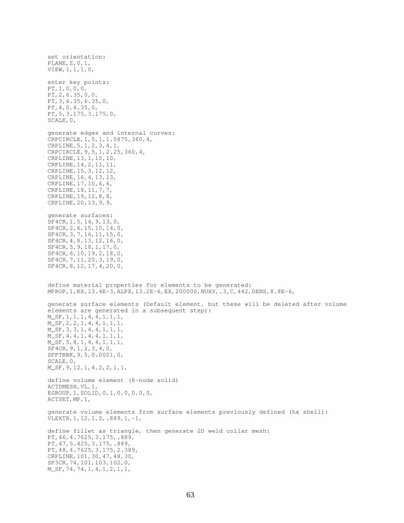
63

set orientation:PLANE,Z,0,1,VIEW,1,1,1,0,

enter key points:PT,1,0,0,0,PT,2,6.35,0,0,PT,3,6.35,6.35,0,PT,4,0,6.35,0,PT,5,3.175,3.175,0,SCALE,0,

generate edges and internal curves:CRPCIRCLE,1,5,1,1.5875,360,4,CRPLINE,5,1,2,3,4,1,CRPCIRCLE,9,5,1,2.25,360,4,CRPLINE,13,1,10,10,CRPLINE,14,2,11,11,CRPLINE,15,3,12,12,CRPLINE,16,4,13,13,CRPLINE,17,10,6,6,CRPLINE,18,11,7,7,CRPLINE,19,12,8,8,CRPLINE,20,13,9,9,

generate surfaces:SF4CR,1,5,14,9,13,0,SF4CR,2,6,15,10,14,0,SF4CR,3,7,16,11,15,0,SF4CR,4,8,13,12,16,0,SF4CR,5,9,18,1,17,0,SF4CR,6,10,19,2,18,0,SF4CR,7,11,20,3,19,0,SF4CR,8,12,17,4,20,0,

define material properties for elements to be generated:MPROP,1,KX,13.4E-3,ALPX,13.2E-6,EX,200000,NUXY,.3,C,442,DENS,8.8E-6,

generate surface elements (Default element, but these will be deleted after volumeelements are generated in a subsequent step):M_SF,1,1,1,4,4,1,1,1,M_SF,2,2,1,4,4,1,1,1,M_SF,3,3,1,4,4,1,1,1,M_SF,4,4,1,4,4,1,1,1,M_SF,5,8,1,4,4,1,1,1,SF4CR,9,1,2,3,4,0,SFPTBRK,9,5,0.0001,0,SCALE,0,M_SF,9,12,1,4,2,2,1,1,

define volume element (8-node solid)ACTDMESH,VL,1,EGROUP,1,SOLID,0,1,0,0,0,0,0,ACTSET,MP,1,

generate volume elements from surface elements previously defined (hx shell):VLEXTR,1,12,1,Z,.889,1,-1,

define fillet as triangle, then generate 2D weld collar mesh:PT,46,4.7625,3.175,.889,PT,47,5.425,3.175,.889,PT,48,4.7625,3.175,2.389,CRPLINE,101,30,47,48,30,SF3CR,74,101,103,102,0,M_SF,74,74,1,4,1,2,1,1,

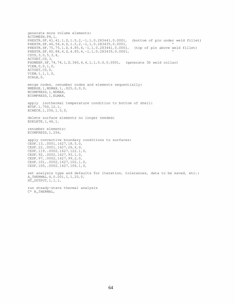
64

generate more volume elements:ACTDMESH,PH,1,PHEXTR,SF,41,41,1,Z,1.5,2,-1,1,0.283441,0.0001, (bottom of pin under weld fillet)PHEXTR,SF,46,54,4,Z,1.5,2,-1,1,0.283435,0.0001, "PHEXTR,SF,75,75,1,Z,4.85,6,-1,1,0.283441,0.0001, (top of pin above weld fillet)PHEXTR,SF,80,88,4,Z,4.85,6,-1,1,0.283435,0.0001, "CSYS,3,0,5,3,4,ACTSET,CS,3,PHSWEEP,SF,74,74,1,Z,360,4,4,1,1,0.6,0.0001, (generate 3D weld collar)VIEW,0,0,1,0,ACTSET,CS,0,VIEW,1,1,1,0,SCALE,0,

merge nodes, renumber nodes and elements sequentially:NMERGE,1,NDMAX,1,.025,0,0,0,NCOMPRESS,1,NDMAX,ECOMPRESS,1,ELMAX,

apply isothermal temperature condition to bottom of shell:NTSF,1,750,12,1,ECHECK,1,256,1,5,0,

delete surface elements no longer needed:EDELETE,1,48,1,

renumber elements:ECOMPRESS,1,256,

apply convective boundary conditions to surfaces:CESF,13,.0001,1627,18,5,0,CESF,22,.0001,1627,26,4,0,CESF,119,.0002,1627,122,1,0,CESF,92,.0002,1627,93,1,0,CESF,97,.0002,1627,99,2,0,CESF,101,.0002,1627,102,1,0,CESF,105,.0002,1627,106,1,0,

set analysis type and defaults for iteration, tolerances, data to be saved, etc.:A_THERMAL,S,0.001,1,1,20,0,HT_OUTPUT,1,1,1,

run steady-state thermal analysisC* R_THERMAL,

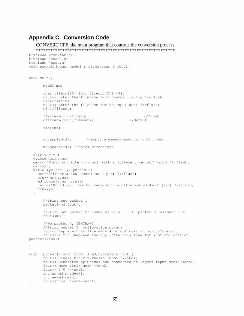
65

Appendix C. Conversion CodeCONVERT.CPP, the main program that controls the conversion process.**********************************************************

#include <fstream.h>#include "model.h"#include "node.h"void packet1(const model & nl,ostream & fout);

void main(){

model md;

char filein[25]={0}, fileout[25]={0};cout<<"Enter the filename from Cosmos listlog "<<flush;cin>>filein;cout<<"Enter the filename for BE input deck "<<flush;cin>>fileout;

ifstream fin(filein); //Inputofstream fout(fileout); //Output

fin>>md;

md.applybc(); //apply element-based bc's to nodes

md.scandir(); //check directions

char yn='y'; double nx,ny,nz; cerr<<"Would you like to check with a different center? (y/n) "<<flush; cin>>yn; while (yn!='n' && yn!='N'){ cerr<<"Enter a new center as x y z: "<<flush; cin>>nx,ny,nz; md.scandir(nx,ny,nz); cerr<<"Would you like to check with a different center? (y/n) "<<flush; cin>>yn; }

//Print out packet 1packet1(md,fout);

//Print out packet 2: nodes w/ bc's & packet 3: element listfout<<md ;

//No packet 4, IEXTRA=0//Print packet 5, collocation pointsfout<<"Replace this line with # of collocation points"<<endl;fout<<"X Y Z Replace and duplicate this line for # of collocation

points"<<endl;

}

void packet1(const model & md,ostream & fout){fout<<"Single Pin Fin Thermal Model"<<endl;fout<<"Generated by Cosmos and converted to Ingber input deck"<<endl;fout<<"More Title Here"<<endl;fout<<"0 0 "<<endl;int nn=md.nnodes();int ne=md.nel();fout<<nn<<' '<<ne<<endl;

}

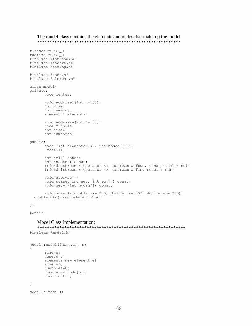
66

The model class contains the elements and nodes that make up the model**********************************************************

#ifndef MODEL_H#define MODEL_H#include <fstream.h>#include <assert.h>#include <string.h>

#include "node.h"#include "element.h"

class model{private:

node center;

void addsizel(int n=100);int size;int numels;element * elements;

void addnsize(int n=100);node * nodes;int sizen;int numnodes;

public:model(int elements=100, int nodes=100);~model();

int nel() const;int nnodes() const;friend ostream & operator << (ostream & fout, const model & md);friend istream & operator >> (istream & fin, model & md);

void applybc();void scaneg(int neg, int eg[] ) const;void geteg(int nodeg[]) const;

void scandir(double nx=-999, double ny=-999, double nz=-999); double dir(const element & e);

};

#endif

Model Class Implementation:************************************************************

#include "model.h"

model::model(int e,int n){

size=e;numels=0;elements=new element[e];sizen=n;numnodes=0;nodes=new node[n];node center;

}

model::~model()

67

{delete [] elements;delete [] nodes;

}

void model::addsizel(int n){

element * larger_array;larger_array=new element[size+n];for (int i=0;i<numels;i++){

larger_array[i]=elements[i];}delete [] elements;elements=larger_array;size += n;

}

void model::addnsize(int n){

node * larger_array;larger_array=new node[sizen+n];for (int i=0;i<numnodes;i++){

larger_array[i]=nodes[i];}delete [] nodes;nodes=larger_array;sizen += n;

}

istream & operator >> (istream & fin, model & md){

//Read in and discard heading line, Node list is firstfin.clear();char line[100];char ready[]="Z-C";do{fin.getline(line,80);cout<<"Node header discard:"<<endl<<line<<endl;}while( ! strstr(line,ready));

//Read in nodes until a failure occurs, indicating element header read://for(int i=nl.numnodes;i<nl.sizen && fin>>nl.nodes[i];i++){for(int i=md.numnodes;fin>>md.nodes[i];i++){

//If numnodes = sizen, then we may have more, so add to sizen//Note we ignore case of an even 100's of nodes, so array could

//inadvertantly get too big, but who cares!md.numnodes++;if (md.numnodes==md.sizen-1){

md.addnsize();}md.center += md.nodes[i]; //sum nodes to find center for surface

check}md.center/=md.numnodes; //average location to find center

//Read in and discard heading line for elementsfin.clear();fin.getline(line,80);cout<<"Element header discard:"<<endl<<line<<endl;

//Read in elements until a failure occurs, indicating eof://for(int i=ell.numels;i<ell.size && fin>>ell.elements[i] && !fin.eof();i++){for(i=md.numels;fin>>md.elements[i] && !fin.eof();i++){

//If numnodes = size, then we may have more, so add to size

68

//Note we ignore case of an even 100's of nodes, so array could//inadvertantly get too big, but who cares!

md.numels++;//cerr<<ell.numels<<' '<<ell.size<<' '<<i<<endl;

if (md.numels==md.size-1){md.addsizel();

}}

return fin;}

ostream & operator << (ostream & fout, const model & md){

//Print packet 2, the nodesfor (int i=0;i<md.numnodes;i++){

fout<<md.nodes[i]<<endl;

}//Print packet 3, the elementsfor (i=0;i<md.numels;i++){

fout<<md.elements[i]<<endl;}

return fout;}

int model::nel() const{

return numels;}

int model::nnodes() const{

return numnodes;}

void model::applybc(){

//This routine applies the boundary conditions found in el to the nodesconst int maxbcs=10;int eg[maxbcs]={0}; //Element group, specifies bc'sint neg=0;int nbdy[maxbcs];int i;double par1[maxbcs];double par2[maxbcs]={0.0};

//First we determin how many element groups there arescaneg(maxbcs,eg);

//Now we get the parameters for each element group:cout<<"Boundary conditions:"<<endl;cout<<"NBDY=1: PAR1=specified T, PAR2=0 "<<endl;cout<<"NBDY=2: PAR1=specified Flux, PAR2=0 "<<endl;cout<<"NBDY=3: PAR1=1/h, PAR2= T inf "<<endl;

for(i=0;i<maxbcs;i++){if (eg[i] != 0){cout<<"For element group "<<eg[i]<<" enter NBDY, PAR1, PAR2: "<<flush;cin>>nbdy[i]>>par1[i]>>par2[i];}

}

//Now we scan elements and apply BC to each node//Array bcapplied is used to look for conflicting bc's applied to same nodeint *bcapplied;bcapplied=new int [numnodes];

69

for( i=0;i<numnodes;i++){bcapplied[i]=0;}

geteg(bcapplied);

//Now we apply the list of BC's to the nodesfor(i=0;i<numnodes;i++){

nodes[i].bc(nbdy[bcapplied[i]],par1[bcapplied[i]],par2[bcapplied[i]]);}

}

void model::scaneg(int neg, int eg[] ) const{ //First we determin how many element groups there are

for (int i=0;i<numels;i++){assert(elements[i].eg() < neg);

eg[elements[i].eg()]=elements[i].eg();}

}

void model::geteg(int nodeg[]) const{

int nlist[9];for(int i=0;i<numels;i++){

elements[i].tellnodes(nlist);for(int j=0;j<9;j++){

if(nodeg[nlist[j]] != 0 && nodeg[nlist[j]] != elements[i].eg()){cerr<<"Conflicting BC: node "<<nlist[j]+1<<" was eg#

"<<nodeg[nlist[j]]<<", requested "<<elements[i].eg()<<" on element "<<i+1<<endl;}else{nodeg[nlist[j]]=elements[i].eg();}

}}

}

void model::scandir(double nx, double ny, double nz){ if (nx != -999){ center=node(nx,ny,nz); }

for (int i=0;i<numels;i++){if(dir(elements[i])<0){

cout<<"Possible orientation problem, element"<<i+1<<endl<<elements[i]<<endl;

}}

cout<<"center was at "<<center.getx()<<' '<<center.gety()<<''<<center.getz()<<endl;}

double model::dir(const element & e){//Return the relative direction of the normal and the vector from the center

//Negative could indicate the element is bass ackwards

//Check element normal direction against center of nodal massdouble nx=0,ny=0,nz=0,cx=0,cy=0,cz=0;double ax,ay,az,bx,by,bz,dp;int nlist[9];

e.tellnodes(nlist);

//Vector from center to 2nd nodecx=nodes[nlist[1]].getx()-center.getx();cy=nodes[nlist[1]].gety()-center.gety();

70

cz=nodes[nlist[1]].getz()-center.getz();//Vector normal to second nodeax=nodes[nlist[1]].getx()-nodes[nlist[0]].getx();ay=nodes[nlist[1]].gety()-nodes[nlist[0]].gety();az=nodes[nlist[1]].getz()-nodes[nlist[0]].getz();bx=nodes[nlist[2]].getx()-nodes[nlist[1]].getx();by=nodes[nlist[2]].gety()-nodes[nlist[1]].gety();bz=nodes[nlist[2]].getz()-nodes[nlist[1]].getz();nx=ay*bz-az*by;ny=az*bx-ax*bz;nz=ax*by-ay*bx;//Dot product to check relative directiondp=cx*nx+cy*ny+cz*nz;return dp;

}

The node class defines the node abstract data type:***************************************************

#ifndef NODE_H#define NODE_H#include <fstream.h>

class node{private:

int nbdy;double par2;double par1;double z;double y;double x;int globalnum;

public:void bc(int btype,double p1,double p2);

friend ostream & operator << (ostream & fout, const node & nd);

friend istream & operator >> (istream & fin, node & nd);node(double nx=0,double y=0, double z=0);void operator += (const node & n);void operator /= (const double & n);double getx();double gety();double getz();

};#endif

#include "node.h"

node::node(double nx, double ny, double nz)

{

x=nx; y=ny; z=nz;

globalnum=nbdy=0;par1=par2=0.0;

}

void node::operator += (const node & n){//Overlaods the += operator to summ nodal locations

x+=n.x;y+=n.y;

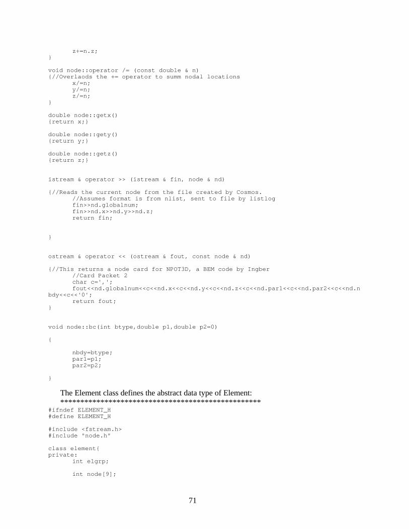
71

z+=n.z;}

void node::operator /= (const double & n){//Overlaods the += operator to summ nodal locations

x/=n;y/=n;z/=n;

}

double node::getx(){return x;}

double node::gety(){return y;}

double node::getz(){return z;}

istream & operator >> (istream & fin, node & nd)

{//Reads the current node from the file created by Cosmos.//Assumes format is from nlist, sent to file by listlogfin>>nd.globalnum;fin>>nd.x>>nd.y>>nd.z;return fin;

}

ostream & operator << (ostream & fout, const node & nd)

{//This returns a node card for NPOT3D, a BEM code by Ingber//Card Packet 2char c=',';fout<<nd.globalnum<<c<<nd.x<<c<<nd.y<<c<<nd.z<<c<<nd.par1<<c<<nd.par2<<c<<nd.n

bdy<<c<<'0';return fout;

}

void node::bc(int btype,double p1,double p2=0)

{

nbdy=btype;par1=p1;par2=p2;

}

The Element class defines the abstract data type of Element:**************************************************

#ifndef ELEMENT_H#define ELEMENT_H

#include <fstream.h>#include "node.h"

class element{private:

int elgrp;

int node[9];

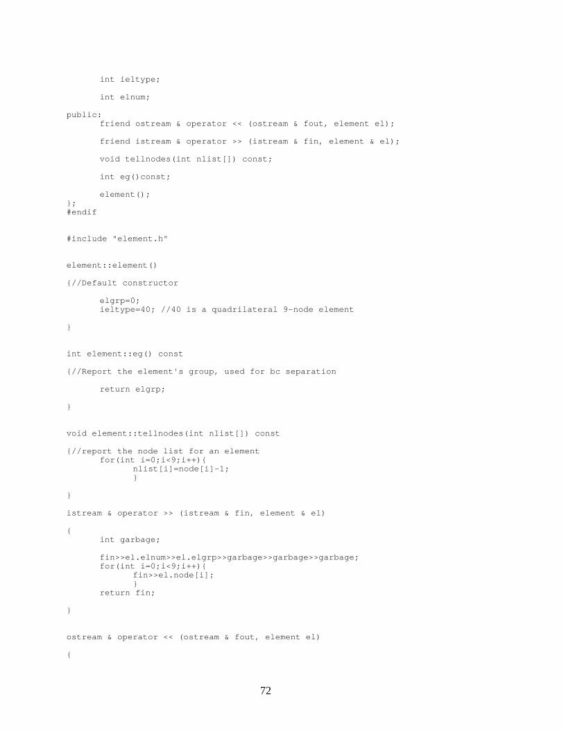
72

int ieltype;

int elnum;

public:friend ostream & operator << (ostream & fout, element el);

friend istream & operator >> (istream & fin, element & el);

void tellnodes(int nlist[]) const;

int eg()const;

element();};#endif

#include "element.h"

element::element()

{//Default constructor

elgrp=0;ieltype=40; //40 is a quadrilateral 9-node element

}

int element::eg() const

{//Report the element's group, used for bc separation

return elgrp;

}

void element::tellnodes(int nlist[]) const

{//report the node list for an elementfor(int i=0;i<9;i++){

nlist[i]=node[i]-1;}

}

istream & operator >> (istream & fin, element & el)

{int garbage;

fin>>el.elnum>>el.elgrp>>garbage>>garbage>>garbage;for(int i=0;i<9;i++){

fin>>el.node[i];}

return fin;

}

ostream & operator << (ostream & fout, element el)

{

73

char c=',';

fout<<el.elnum<<c<<el.ieltype;for (int i=0;i<9;i++){

fout<<c<<el.node[i];}

return fout;

}

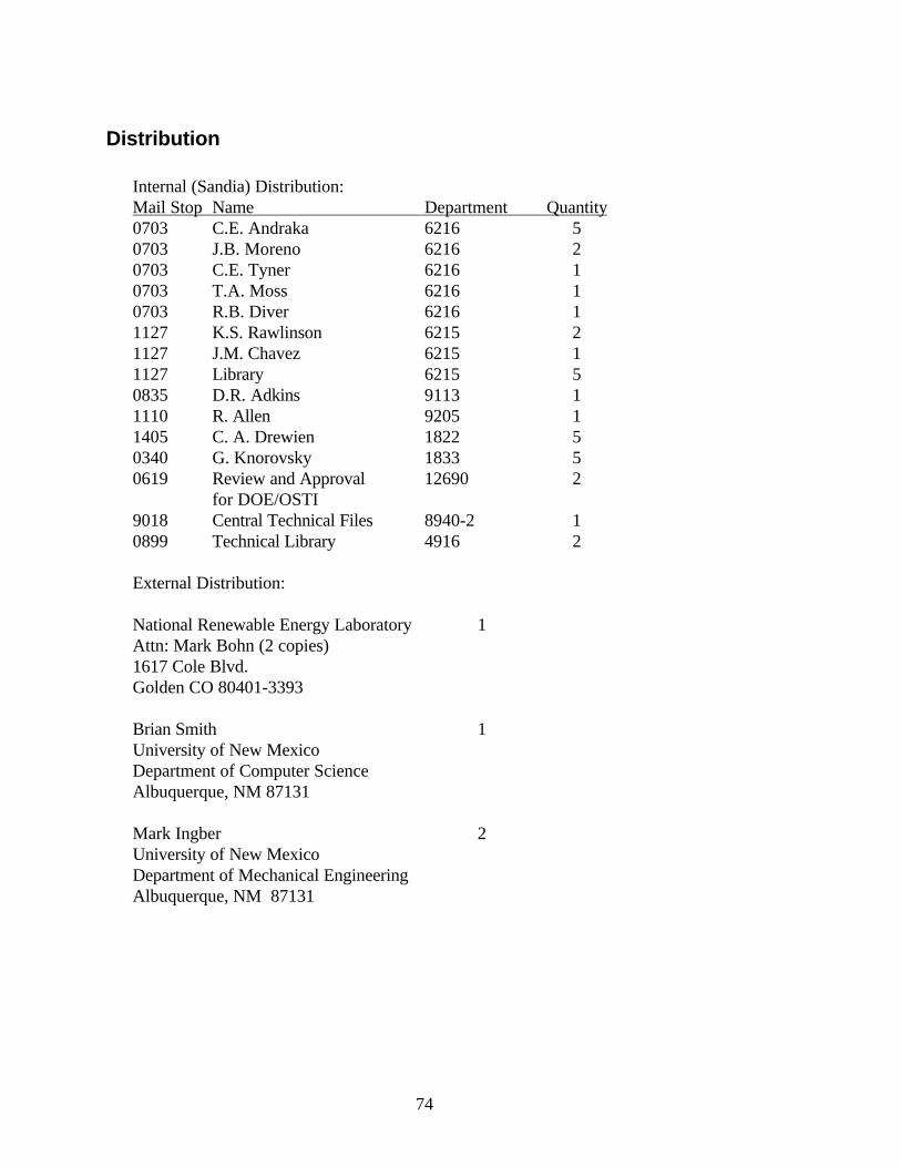
74

Distribution

Internal (Sandia) Distribution:Mail Stop Name Department Quantity0703 C.E. Andraka 6216 50703 J.B. Moreno 6216 20703 C.E. Tyner 6216 10703 T.A. Moss 6216 10703 R.B. Diver 6216 11127 K.S. Rawlinson 6215 21127 J.M. Chavez 6215 11127 Library 6215 50835 D.R. Adkins 9113 11110 R. Allen 9205 11405 C. A. Drewien 1822 50340 G. Knorovsky 1833 50619 Review and Approval 12690 2

for DOE/OSTI9018 Central Technical Files 8940-2 10899 Technical Library 4916 2

External Distribution:

National Renewable Energy Laboratory 1Attn: Mark Bohn (2 copies)1617 Cole Blvd.Golden CO 80401-3393

Brian Smith 1University of New MexicoDepartment of Computer ScienceAlbuquerque, NM 87131

Mark Ingber 2University of New MexicoDepartment of Mechanical EngineeringAlbuquerque, NM 87131