Engineering Analysis with Boundary Elements 37 (2013) 977–987

Contents lists available at SciVerse ScienceDirect

Engineering Analysis with Boundary Elements

0955-79http://d

n CorrE-m

journal homepage: www.elsevier.com/locate/enganabound

Boundary element model for electrochemical dissolution underexternally applied low level stress

Bruce M. Butler a, Manoj B. Chopra b, Alain J. Kassab c,n, Vimal Chaitanya d

a Walt Disney World Co., Orlando, FL, USAb Department of Civil, Environmental and Construction, Engineering, University of Central Florida, Orlando, FL, USAc Department of Mechanical, Materials, and Aerospace Engineering, University of Central Florida, Orlando, FL, USAd New Mexico State University, Las Cruces, NM, USA

a r t i c l e i n f o

Article history:Received 23 January 2013Accepted 15 March 2013Available online 28 April 2013

Keywords:BEMCorrosionStress

97/$ - see front matter & 2013 Elsevier Ltd. Ax.doi.org/10.1016/j.enganabound.2013.03.010

esponding author. Tel.: +1 4078235778.ail address: alain.kassab@ucf.edu (A.J. Kassab)

a b s t r a c t

The effects of low levels of stress on the dissolution rate of type 304 stainless steel in seawater aredetermined, and these effects are incorporated into a boundary element method (BEM) code which waswritten to predict long-term changes in geometry, including those due to the stress-modified dissolutionrates. Corrosion in the absence of stress effects is thoroughly documented, while the effects ofmicromechanical damage caused by strains in the plastic region are also well recognized. However,very little is known regarding the effects of low levels of stress (in the elastic region) on the behavior ofdissolution rates of metals in general. To quantify this effect, a system consisting of stainless steel inseawater was chosen as the subject of this investigation.

An initial set of controlled experiments using nearly pure copper with NHOH electrolyte was used totest the experimental methods developed for this study and to verify the functionality of the numericalcode in predicting large changes in geometry due to long duration dissolution. The numerical code isbased on the BEM to predict the electrochemical dissolution activity in 2D and in 3D-axisymmetricgeometries with nonlinearities in the response to stress and the boundary conditions given by the highlynon-linear polarization response of the specimen. A Newton–Raphson iterative procedure is used tosolve for equilibrium at each solution step. In the BEM code, a nodal optimization routine dynamicallymodifies the number of nodes and their location on the boundary, which is required by the large changesin geometry experienced during long duration dissolution. New SE-elements are developed to modelsections of the boundary where nodes are dynamically located, defined by a curvilinear fit usingorthogonal Chebyshev polynomials through previous nodal locations. The code links stress and potentialtype corrosion formulations to generate geometrical changes due to stress and corrosion. Polarizationcurves were measured and input into the BEM code and recession profiles were predicted. Comparisonbetween experiment and predictions reveal that, given the polarization curves measured in the lab, theBEM code predicts accurate recession profiles.

Once the laboratory methods and computer program were verified, a second electrochemical system isadopted to study the effects of stress in the linear range upon recession rates. This system consists of type304 stainless steel in simulated seawater subjected to compressive and tensile stresses up to 20% of yield.

Comparison between numerical predictions using polarization curves determined by experiment for thecopper/ammonium system reveals that the BEM code developed to model recession of corroding surfacesfaithfully reproduces the recession fronts measured in the experiments. Furthermore, it is shown in a seriesof repeatable laboratory tests, in the stainless-steel/saline system, that stress in the linear range indeed affectsthe polarization curves for different levels of stress and, furthermore, it is found that the shift in thepolarization curve depends on stress rate.

& 2013 Elsevier Ltd. All rights reserved.

1. Introduction

This paper presents the effects of low levels of stress (in theelastic range) on the dissolution rate of metals by means of

ll rights reserved.

.

experiments. The results are then incorporated into a boundaryelement program to predict recession rates of corroding structures.Corrosion, ignoring the effects of stress, is thoroughly documented,and the effects of micromechanical damage caused by strains in theplastic region are well recognized. However, very little is knownregarding the effects of low levels of stress on the behavior ofmetals in general. To quantify this effect the system consisting ofstainless steel in seawater was investigated. The two primary

B.M. Butler et al. / Engineering Analysis with Boundary Elements 37 (2013) 977–987978

aspects of this research are the experimental determination of theeffects of low level stresses on the corrosion behavior of samplesand the incorporation of these effects in a boundary elementmethod-based code which was written to predict long-termchanges in geometry due to the stress modified dissolution.

The initial experimental system used is high purity copper withaerated NH4OH as the electrolyte. Copper was selected due to itsrelatively low cost, because it is thermodynamically reactive,undergoes dissolution at room temperature, and it has been thesubject of numerous studies. It can easily be obtained in singlecrystal, foil, thin plate, and poly-crystalline form in purities of upto 99.99%. This system is used to verify the functionality of thenumerical code in predicting large changes in geometry due tolong-duration dissolution. The high purity copper eliminatedpotential non-homogenieties of the material resulting in localfluctuations in the polarization responses. Two different axisym-metric geometries were investigated, a solid copper disk anodewith a graphite cathode and a large copper plate anode with agraphite cathode. Analysis of time-dependent measurements ofthe specimens yields the geometry changes in the corrosion regionas a function of time. Using a quasi-equilibrium analysis, combin-ing the geometrical changes and the total current yields averagecurrent density on the surface as a function of time. That is, atevery step in time, a Laplace equation is solved for the potentialand the current density at the surface of the body, and a kinematicequation is used to move the boundary of the corroding regionuntil the next time measurement of the polarization curve.Comparison of predicted and measured recession rates are shownto be in agreement, thus validating the approach.

The second electrochemical system used is type 304 stainlesssteel in a saline electrolyte which simulates seawater composition.This grade of stainless steel can vary from batch to batch and willcontain spot impurities and, thus, it does not provide the samecontrol over chemical composition afforded by a pure coppersystem. However, it is the most common grade of stainless steelused for applications designed to carry loads. Furthermore, salineenvironments are quite common, especially in the coastal regionsof Florida. Thus, the combined system is representative of commonmaterial and environment encountered in engineering design ofpotentially corroding structures.

In practice, all properly designed statically loaded structuresexperience a maximum stress of approximately 60% of yield, andthey are, during the majority of their service life, subjected tostresses in the 5–20%-of-yield range, either tension or compres-sion. Properly designed cyclically loaded structures are subjectedto repetitive stress ranges of approximately715% of yield. Thus,this research into the effects of low stress (720% of yield) on thecorrosion behavior is of significant and immediately practicalvalue. A four-point bend test of specimen immersed in a salinesolution is undertaken to investigate this effect.

A boundary element method code is written to predict theelectrochemical dissolution activity in 2D and axisymmetric geo-metries of partially corroding systems. The nonlinearities in thisproblem are due to boundary conditions of the third kind in whichthe ratio of the potential to the current density at the corrodingsurface is provided as highly non-linear polarization curve mea-sured by experiment. This curve is particular to each specimen,electrolytic environment, stress, time, and potential other factors,such as temperature, which are not considered in this study. Inthis study, two different corroding specimens in two differentelectrolytic environments under varying levels of stress are con-sidered. A Newton–Raphson iterative procedure is used to solvefor equilibrium at each solution step. In the BEM code, a nodaloptimization routine dynamically modifies the number of nodesand their location on the boundary. This is necessary due to thelarge changes in geometry experienced during long duration

dissolution. The term “super-element” is used to denote onesection of the boundary where nodes are dynamically locatedalong the boundary and which is defined by a curvilinear fitthrough the previous nodal locations. Corners, edges, and othergeometrically important features as well as changes in materialproperties occur only at the juncture of super-elements. Since anysuper-element may be subject to complex changes in geometry, itwas necessary to describe all elements in a parametric sense. A fitconsisting of orthogonal Chebyshev polynomials was found to besufficiently smooth for the parametric representation of the datapoints.

Comparison between numerical predictions using polarizationcurves determined by experiment for the copper/ammoniumsystem reveals that the BEM code developed to model recessionof corroding surfaces faithfully reproduces recession fronts mea-sured in the experiments. Furthermore, it is shown in a series ofrepeatable laboratory tests, in the stainless-steel/saline system,that stress in the linear range indeed affects the polarizationcurves for different levels of stress and, furthermore, it is foundthat the shift in the polarization curve depends on stress rate.

2. Background

Electrochemical corrosion, resulting in cracking or increaseddissolution rates, may involve two types of applications, namelybiomedical and structural. Metals have been used successfully forbiomedical applications for years with the most common struc-tural materials being stainless steel, cobalt–chromium alloys, andtitanium, Donachie [1]. All types of corrosion have been observedon bio-materials in the body: general corrosion, pitting and crevicecorrosion, stress-corrosion cracking, corrosion fatigue, and inter-granular corrosion. Biomedical applications of the effects ofcorrosion have been studied by Klein [2], Yano et al. [3] andMorita [4]. Structural applications of stainless steel are exceedinglycommon, see [5], and the effects of high stress levels on crackingsusceptibility have also been studied. The primary degradationmechanisms identified during operation times are intergranularstress corrosion cracking (IGSCC) and irradiation assisted stresscorrosion cracking (IASCC). Onchi et al. [6] discuss type 304stainless-steel samples that have been solution annealed, irra-diated and then raised to a stress level of 311–546 MPa to quantifythe increased susceptibility to IASCC. Quan [7] presents results ofstudies on hydrogen migration into the metal crystal lattice of highstrength low alloy (HSLA) materials under the influence of stressfields. Previous results indicate that the while a constant stressdoes not affect the hydrogen diffusion coefficient, it does increasethe saturated diffusion flux.

Changes in the corrosion resistance via shifting of the polariza-tion response to stress in a Ringer's solution electrolyte are studiedby Bundy et al. [8]. Biomechanics literature reveals several reportsof maximum applied stress levels of 400–500 MPa and the stressintensity factors chosen in this study reflect these loading condi-tions, close to but just short of rapid fracture. It is clearlydemonstrated that applied polarization and stresses resulting inplastic strains may cause a higher rate of dissolution due to a lessstable passive film. It is concluded that the difference between thestressed and unstressed specimens was due only to the existenceof plastic deformation in the stressed samples and that significantplastic deformation occurred at all stress levels tested. Navai [9]and Navai and Debbouz [10] studied the influence of stress on thecomposition of passive films formed on 302 stainless-steel alloys.Bundy et al. [11] reported that alterations in the characteristics ofthe passive film were present even up to 20 weeks after applica-tion of stress. Application of a stress level mechanically disrupts or

B.M. Butler et al. / Engineering Analysis with Boundary Elements 37 (2013) 977–987 979

increases the ionic conductivity of any passive film which wasinitially present.

In all cases cited above, the stress levels investigated were close toor above yield stress. In many prosthetic uses of biomedical materialsfor leg or hip reinforcement these high stress levels are justified.However, there are many of uses of biomedical materials, specificallystainless-steel, where the stress levels encounter are of a much lowervalue. In all properly designed structural applications, the stresslevels typically experienced are much lower than yield. Furthermore,stainless-steel structures are not stressed in the plastic range undernormal conditions and are often subjected to corrosive environments,such as coastal regions. Thus the specific issues of changes inpolarization behavior due to low stress levels are important, andare the main emphasis of this paper.

Fultz et al. [12] studied the detection of potential fields due tocoating defects and eddy current detection of cracks using highfrequency magnetic fields to detect cracks. However very littleinformation exists on the direct interaction between strain andpotential fields in a corrosion system. Maugin [13] investigated themechanism in piezoelectric materials where the presence of straininduces a change in electric polarization. Moon [14] points out thatthe coupling between strain and the electric field occurs only indielectrically anisotropic materials. Al-Hassani [15] discusses theproblem of buckling under the influence of large (relative to theelastic stiffness) magnetic fields. In practical terms, these effectsare limited to structures which undergo significant deformations,on the order of magnitude of the dimensions of the structuralmembers. To summarize, for the class of problems dealt with inthis research, specifically long-term low current corrosion actingon conducting solids:

(1)

Changes in the strain field which do not result in largedeformations of the electrode (buckling) will not result inchanges to the potential field in the electrolyte.

(2)

The potential, electric, and resulting magnetic fields are ofsuch magnitude compared to the elastic stiffness and mass ofthe electrode that the strain fields induced in the electrode areessentially insignificant.

BEM is adopted because it does not require discretization of thedomain with internal elements in comparison to other conven-tional analysis techniques, e.g. finite-difference-method (FDM) andfinite-element-method (FEM). The knowledge of physical quanti-ties (potential and current density) on the surface of corrodingmaterials is important in corrosion problems. Fu and Chow [16]introduced the use of a boundary integral formulation of theLaplace equation to solving corrosion problems. They modeled anaxisymmetric problem and compared to experimental results ofpotential and current distributions. The behavior of the electrodedouble layer, where the electroneutrality law is not valid, wasexpressed as an experimentally determined polarization curve,and the Laplace equation is applied only to the bulk electrolyte.This is the most common approach taken by researchers inmodeling corrosion, and has also been adopted in the presentstudy. A detailed review of the literature associated with theapplication of BEM to corrosion problems is provided in Butler[17]. Recently, Butler et al. [18] presented a boundary elementmodel for the large scale changes in geometry due to electro-chemical dissolution of polycrystalline pure copper. Using a non-linear polarization curve determined from experiments andimposed as a third kind boundary condition, a quasi-static analysiswas conducted and the numerical model predictions of largechanges in geometry due to corrosion were compared to experi-mental findings. The BEM code predicted the recession profilesaccurately. This paper describes the effect of low-level stresson the dissolution rates of stainless steel in seawater using

experimentally-determined polarization curves and an axisym-metric BEM model.

3. Governing equations

The governing transport equations, boundary conditions, corro-sion models and a discussion of the treatment of moving bound-aries were presented in Butler [17] and Butler et al. [18]. Thebehavior of an electrochemical system is modeled using theLaplace equation for the electric field potential ϕ, using thefollowing equation:

∇2ϕ¼ 0 ð1ÞMass transport considerations are neglected since in typicalcorrosion systems where neither the electrolyte nor the electrodesare thin films, the behavior tends to bulk electrolyte behaviorwhen the electrolyte is thicker than 0.1–0.3 cm. The conductivityof the metal is assumed infinite and only the electrolyte ismodeled. Further, as the electromagnetic field changes graduallyover time, a quasi-static model provided by Eq. (1) is adequate. Theexperiments carried out in this study involved periods of the orderof several weeks. The above equation is solved using the boundaryelement method for axisymmetric systems. In particular, forpurely axisymmetric problems, the governing boundary integralequation can be expressed as [19,20]

cðξÞΦðξÞ þZΓ−ΦðxÞ qnðξ; xÞ dΓ ðxÞ ¼

ZΓΦ

nðxÞ qðξ; xÞ dΓ ðxÞ ð2Þ

where cðξÞ is equal to one when ξ lies within the domain and 1/2 isξ is on a smooth boundary. The generating curve for the axisym-metric body is denoted by Γ . Here, the axisymmetric kernels aredefined as

Φnðξ; xÞ ¼ 4KðmÞffiffiffiffiffiffiffiffiffiffiffiffi

aþ bp ð3Þ

qnðξ; xÞ ¼ 4ffiffiffiffiffiffiffiffiffiffiffiffiaþ b

p 12rðxÞ

R2ðξÞ−R2ðxÞ þ ½ZðξÞ−ZðxÞ�2a−b

EðmÞ−KðmÞ" #

ηrðxÞ(

þ ZðξÞ−ZðxÞa−b

EðmÞηzðxÞ�

ð4Þ

Here, K(m) is the complete elliptic integral of the first kind,E(m) is the complete elliptic integral of the second kind, ηrðxÞ andηzðxÞ are the direction cosines of the outward drawn normal to thegenerating curve, a¼ r2ðξÞ þ r2ðxÞ þ ½zðξÞ−zðxÞ�2, b¼ 2rðξÞrðxÞ;m¼2b=ðaþ bÞ, and rðxÞ and zðxÞ are the polar coordinates [21]. Using astandard boundary element method, the above equation can bediscretized and solved for the given boundary conditions. In ourcode, a library of elements is available ranging from constant tofourth order isoparametric boundary elements. Quadratic ele-ments are usually used in all numerical analyses.

For electrochemical models, the field variable is the electro-chemical potential in the system and its derivative is proportionalto the current density (the proportionality constant being theconductivity of the electrolyte), i.e. at the anodic or cathodicsurface the relation

k∂ϕ∂n

¼ hðϕÞϕ ð5Þ

is used to model the boundary condition. Polarization curves, plotsof ∂ϕ=∂n vs. ϕ, which provide the function hðϕÞ, are determinedfrom experiments. This Robin boundary condition is nonlinear, andresolution of the potential field thus requires iteration. Initially, apotential distribution is assumed on Γ, then a solution obtainedand the resulting fluxes calculated. These fluxes, after beingmultiplied by the electrolyte conductivity to yield current densi-ties, were compared to the current densities calculated from the

Table 1Chemical analysis of stainless steel specimen.

Composition % (by weight)

Iron 71.355

B.M. Butler et al. / Engineering Analysis with Boundary Elements 37 (2013) 977–987980

polarization data. A Newton–Raphson iterative procedure wasused to solve this nonlinear boundary condition problem.

The analysis of moving fronts, such as those arising in Stefanproblems, normally require a transient formulation [21]. Themoving boundary problem considered in this paper is quasi-static due to the nature of the field described above. At the endof each time step, the resulting flux distribution is known. Since∂ϕ=∂n¼ k J

!, where k is the conductivity of the electrolyte, and J

!is the current density, the resultant current density along eachelement is determined. At each node the integral of currentdensity from the adjacent elements is calculated, to give the meancurrent density in the neighborhood of the node. Faraday's law isthen used to determine the dissolution resulting from the meancurrent density and the quantity of time represented by the timestep as

m¼ ItanF

ð6Þ

where m is the mass reacted per unit area, I is the current density,t is the duration of the time step in seconds, a is the atomic weightof the metal, n is the number of electrons released by an atomreleased from the lattice, and F is the Faraday constant 96,500Coulombs/n. The direction of node movement is in the normalizeddirection of the vector sum of the fluxes. Movement in bothdirections is possible, simulating dissolution and plating.

Further details of the approach adopted to handle movingboundaries using a super-element are provided in Butler et al.[18]. The term “super-element” is used to denote one section ofthe boundary where nodes are dynamically located along theboundary and which is defined by a curvilinear fit through theprevious nodal locations. The complex changes in geometrynecessitated parametric descriptions of all elements. A fit consist-ing of orthogonal Chebyshev polynomials was found to be suffi-ciently smooth for the parametric representation of the datapoints. This approach allows a very fast modification of thenumber of nodes and their locations. Because the number andlocation of nodes within a super-element are dynamicallyadjusted, the order of the elements within a super-element iseasily changed as well. This gives the BEM code tremendousflexibility as the number of nodes, location of nodes, and orderof the elements can vary with location on the boundary andwith time.

Carbon 0.042Manganese 1.68Phosphorus 0.019Sulfur 0.024Silicon 0.30Chromium 17.70Nickel 8.36Molybdenum 0.52

Table 2Potentiodynamic scan configuration.

Software EG& G Model 352/252Corrosion Measurement & Control

Hardware EG &G Model 273 PotentiostatFilter 590 Hz low pass filter on the currentType of scan POTENTIODYNAMICReference electrode SCE

4. Numerical implementation

Using conventional BEM practice, by introducing the discreti-zations of the boundary, the potential, and its normal derivativeinto the boundary integral equations, the boundary elementequations are derived in the following standard form:

½H�fϕg ¼ ½G�fqg ð7Þwhere fϕg is the vector of nodal values of the potential, fqg is theset of nodal values of the normal derivative of the potential, whilethe influence matrices ½H� and ½G� are computed numerically usingGauss-type quadratures. Upon specification of the boundary con-ditions, the above are solved for the unknowns to finally deter-mine both the potential and its normal derivative everywhere atthe boundary.

Step increment 1 mVScan rate 0.5 mV/sStep time 2 sCurrent range AutoCurrent interrupt OnIR interval 2 sRise time High StabilityArea of specimen 3.629 sq. cmLine sync No

5. Experimental determination of polarization curves

A series of low stress (0–40 MPa) tests were conducted undercompressive stresses to measure the change in polarizationresponse to stress. To minimize disruption of the passive filmcharacteristics, these experiments monitored the change in the

open-circuit potential as a function of stress and stress rate. Fourpoint bend specimens were used to provide a constant stressregion thus allowing precise correlation between stress level andchanges in polarization characteristics.

5.1. Measurement of the polarization response

The specimens used in the four point bend tests, measured1.00 in. wide �0.500 in. thick �7.0 in. long and are composedof type 304 austenitic stainless steel with the composition asindicated in Table 1. All specimens were annealed by raising theirtemperature to 650 1C and then allowing them to slowly cool inthe oven (cooling rate approximately 40–55 1C/h). The electrolyteis a 2.54% solution of NaCl in distilled water to simulate seawater.The temperature was a relatively constant 26 1C and the solution isconsidered to be aerated but quiescent. The surface of the speci-men was coated with a two layer system, a primer/epoxy coatingwhich was then covered by a polyvinyl film, with a 1.905 cm�1.905 cm exposed region at the center of the specimen. Theexposed region was polished using finer grades of silicon carbideabrasives until a mirror finish had been achieved. All specimenswere immersed in the electrolyte for 160 h prior to any scans. Thespecific configuration parameters for these scans are shown inTable 2.

Three typical polarization curves for this specimen are shownin Fig. 1, and the mean polarization curve for the zero load case isgiven in Fig. 2.

The equations describing the best-fit through the data shownin Fig. 2 are listed below:

ianodic½ϕ� ¼ þ 10−6:74−0:432nsinh−1ð1900nðϕþ0:514ÞÞ ð8Þ

icathodic½ϕ� ¼−10−6:74−0:500nsinh−1ð1170nðϕþ0:514ÞÞ ð9Þ

-0.6

-0.58

-0.56

-0.54

-0.52

-0.5

-0.48

-0.46

-0.44

-0.42

-0.4

-7 -6.5 -6 -5.5 -5 -4.5 -4Log (current density - amps/cm^2)

Polarization Curves - Zero Stress Condition

Pot

entia

l (vo

lts)

No Load02.txtNo Load03.txtNo Load04.txt

Fig. 1. Polarization response—zero stress.

-0.6

-0.58

-0.56

-0.54

-0.52

-0.5

-0.48

-0.46

-0.44

-0.42

-0.4-7 -6.5 -6 -5.5 -5 -4.5 -4 -3.5

Log (current density -amps/cm^2)

Polarization Curves - Zero Stress ConditionSymmetrical Anodic & Cathodic Butler-Volmer Curves

Pot

entia

l (vo

lts)

Mean Value of 3 Scans

Cathodic Curve asSymmetrical Anodic Curve

Divergence from measured data

Fig. 2. Symmetric polarization curves for the zero load mean.

B.M. Butler et al. / Engineering Analysis with Boundary Elements 37 (2013) 977–987 981

Because the anodic and cathodic potential-current densityrelationships are not quite symmetric, the condition known asfaradaic rectification is present.

5.2. Measurement of the effect of stress on the polarization response

5.2.1. Testing methodologyAs an initial step, three polarization curves generated for a

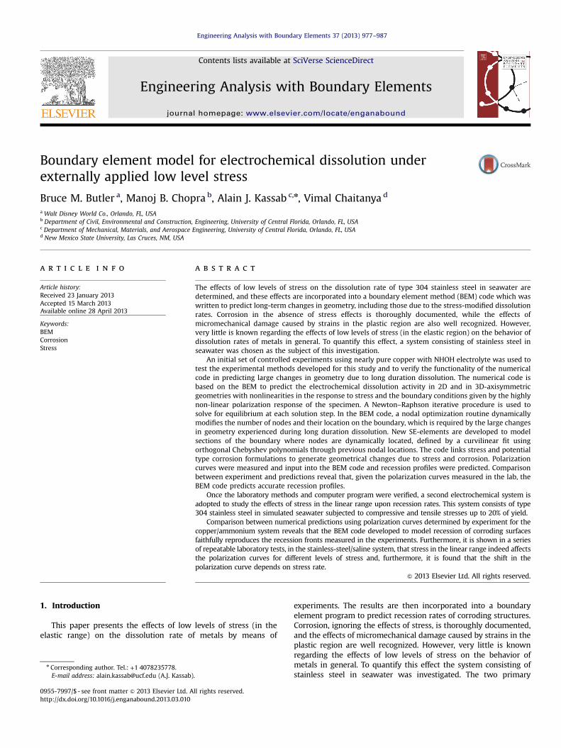
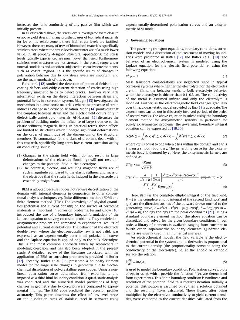
specimen at different stress levels is shown in the Evans diagramof Fig. 3, where it can be seen that the Tafel slopes of the curves arenot appreciably changed. There is a very slight trend in themagnitude of the exchange current density, but as this has verylittle effect on the corrosion rate at any meaningful deviation fromEcorr and may be due to subtle changes in the surface profile frompreceding scans, it is not considered significant.

Because the potentiodynamic scans indicated that the Tafelslopes of the polarization curves did not change, the appropriatescanning technique was chosen to correlate Ecorr vs. time. In thistechnique, the potentiostat varies the potential as required tomaintain the exchange current density as a function of time.Normally this technique is used to determine the time requiredfor stabilization of a specimen when immersed in a solution, oncethis stabilization has occurred, there is no change in Ecorr. The

advantage of using this technique over a complete potentiody-namic scan is that there is no effect on the surface of the specimen,which is present when polarizing far above/below Ecorr, andchanges in the surface profile which may affect the polarizationresponse are avoided.

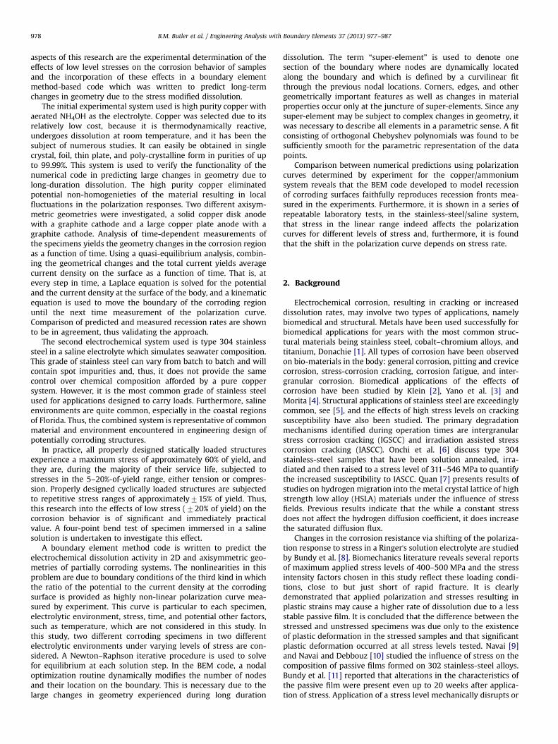
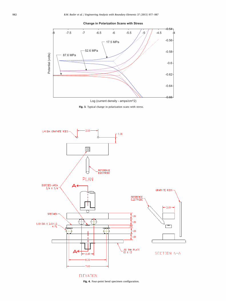
To clearly measure the effect of the stress field and the rate ofchange of stress on the current/potential relationship (the polar-ization function) a constant stress field in the area being measuredis desirable. To achieve this a four-point bend test was constructed.The configuration is shown in Fig. 4. Although elaborate measureswere taken to isolate the apparatus from the sample, to furthereliminate any potential for galvanic currents, all pieces of theequipment were constructed of the same material as the specimen(type 304 stainless steel). Initial experiments were affected by agalvanic couple between the copper wire which provides theelectrical path from the specimen to the potentiostat and thespecimen itself, which was traced to migration of trace quantitiesof the electrolyte through the insulation surrounding the wire.This problem was solved by using 0.032 in. diameter type 304stainless-steel insulated wire as the conductive path.

Due to the extremely low equilibrium currents, electricalisolation was of critical importance. Each individual piece of theapparatus was coated with a polyvinyl film and as an additional

-0.66

-0.64

-0.62

-0.6

-0.58

-0.56

-0.54-8 -7.5 -7 -6.5 -6 -5.5 -5 -4.5 -4

Log (current density - amps/cm^2)

Change in Polarization Scans with Stress

Pot

entia

l (vo

lts)

17.5 MPa

52.6 MPa87.6 MPa

Fig. 3. Typical change in polarization scans with stress.

Fig. 4. Four-point bend specimen configuration.

B.M. Butler et al. / Engineering Analysis with Boundary Elements 37 (2013) 977–987982

B.M. Butler et al. / Engineering Analysis with Boundary Elements 37 (2013) 977–987 983

precaution Teflon sheets were placed between each piece (includ-ing the MTS machine). The configuration is shown in Fig. 5.

The specific configuration parameters for the scans relatingEcorr to stress and stress rate are shown in Table 3.

Table 3Ecorr vs. time scan configuration.

Software EG&G Model 352/252 Corrosion Measurement & ControlHardware EG&G Model 273 PotentiostatFilter 590 Hz low pass filter on the currentType of scan Ecorr vs. timeReference electrode SCEStep increment n/aScan rate n/aTime/Pt 1 sCurrent range n/aCurrent interrupt n/aIR interval n/aRise time n/aArea of specimen n/aLine sync n/a

5.3. Compression face bending stress

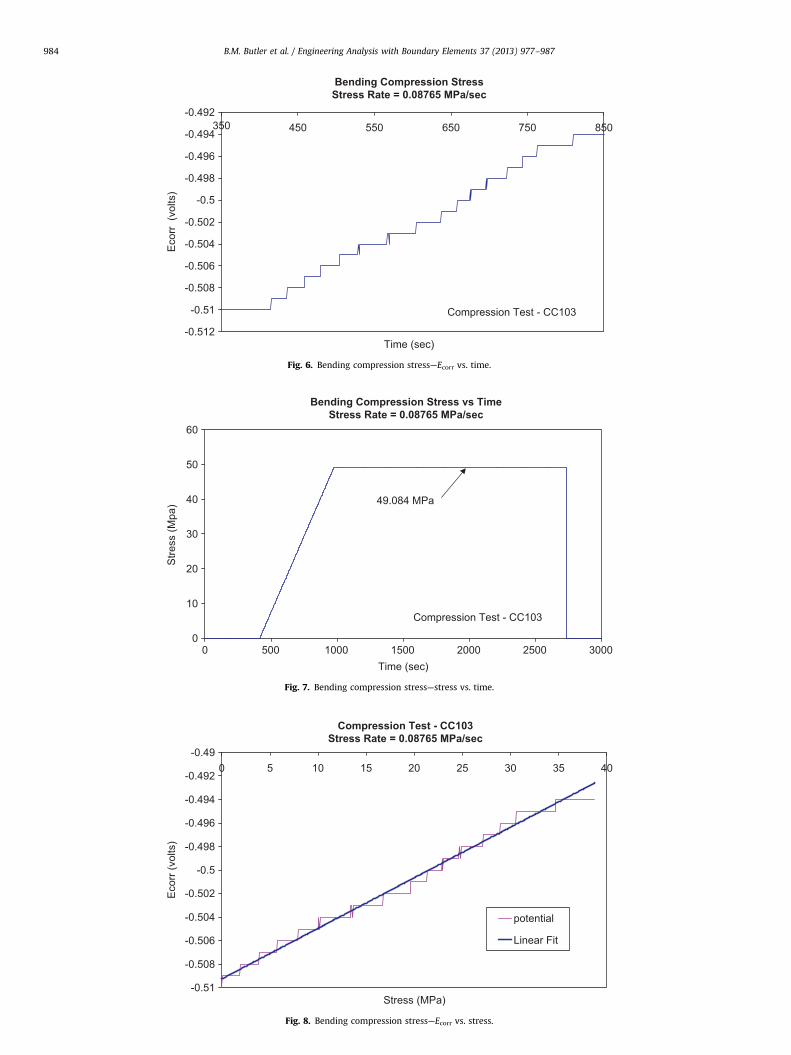
A typical scan of a specimen subjected to compressive stressesover the exposed region is shown in Fig. 6. Notice that due to the1 mV maximum resolution of the potentiostat, the scan appears asa step function. The stress was applied at a constant rate and it canbe seen that for a constant rate of stress increase, the correspond-ing change in Ecorr is constant.

Fig. 7 shows the variation of compressive stress with time andFig. 8 shows the relationship between compressive stress and Ecorrfor a specimen subjected to a compressive stress increasing at arate of 0:08765 MPa=s. For the region 0 ≤s≤40 MPa there is alinear relationship between stress and Ecorr; however, beyond thislevel there is no further change in Ecorr. This upper limit was foundto be consistently at the 40–50 MPa which is approximately 20–25% of the yield point.

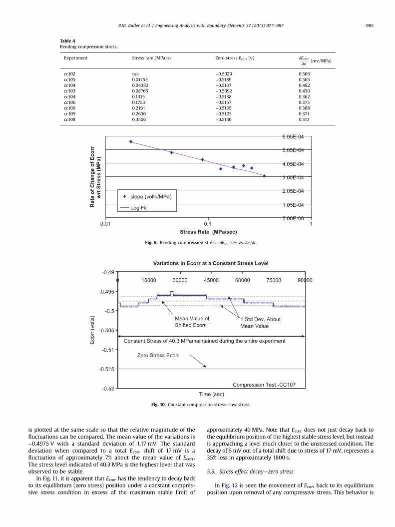
Figs. 6–8 are specific to experiment CC-103, and the resultsfrom it as well as eight other runs at differing stress rates, arelisted in Table 4. All the data clearly showed a linear relationshipbetween stress and shifts in Ecorr, furthermore, as clearly be seen inFig. 9, there is a correlation between ∂Ecorr=∂s and ∂s=∂t. Thisfunctional relationship between Ecorr, ∂Ecorr=∂s, and ∂s=∂t is

Fig. 5. Four-point bend specim

quantified in the equation below

δEcorr ¼ 3:708� 10−4scomp−1:882� 10−4 Log∂scomp

∂t

� �ð10Þ

for 0 ≤scomp ≤40 MPa we have 0≤∂scomp=∂t≤0:35 MPa=s, whereδEcorr is the change in equilibrium potential in volts, scomp is thecompressive stress in MPa, ∂scomp=∂t is the stress rate in MPa/s.

5.4. Stress effect decay—constant stress

In Fig. 10, it can be seen that for low compressive stresses thereis some random variability in the equilibrium potential, Ecorr,however, the shift due to stress remains consistent. Note that it

en isolation methodology.

-0.512

-0.51

-0.508

-0.506

-0.504

-0.502

-0.5

-0.498

-0.496

-0.494

-0.492350 450 550 650 750 850

Time (sec)

Bending Compression StressStress Rate = 0.08765 MPa/sec

Eco

rr (

volts

)

Compression Test - CC103

Fig. 6. Bending compression stress—Ecorr vs. time.

0

10

20

30

40

50

60

0 500 1000 1500 2000 2500 3000Time (sec)

Bending Compression Stress vs TimeStress Rate = 0.08765 MPa/sec

Stre

ss (M

pa)

Compression Test - CC103

49.084 MPa

Fig. 7. Bending compression stress—stress vs. time.

-0.51

-0.508

-0.506

-0.504

-0.502

-0.5

-0.498

-0.496

-0.494

-0.492

-0.490 5 10 15 20 25 30 35 40

Stress (MPa)

Compression Test - CC103Stress Rate = 0.08765 MPa/sec

Eco

rr (v

olts

)

potential

Linear Fit

Fig. 8. Bending compression stress—Ecorr vs. stress.

B.M. Butler et al. / Engineering Analysis with Boundary Elements 37 (2013) 977–987984

Table 4Bending compression stress.

Experiment Stress rate (MPa=sÞ Zero stress Ecorr (v) ∂Ecorr∂s

(mv=MPa)

cc102 n/a −0.5029 0.506cc105 0.01753 −0.5189 0.565cc104 0.04382 −0.5137 0.482cc103 0.08765 −0.5092 0.430cc104 0.1315 −0.5138 0.362cc106 0.1753 −0.5157 0.375cc109 0.2191 −0.5135 0.388cc109 0.2630 −0.5125 0.371cc108 0.3506 −0.5140 0.313

5.00E-06

1.05E-04

2.05E-04

3.05E-04

4.05E-04

5.05E-04

6.05E-04

0.10.01 1Stress Rate (MPa/sec)

Rat

e of

Cha

nge

of E

corr

wrt

Str

ess

(MPa

)

slope (volts/MPa)

Log Fit

Fig. 9. Bending compression stress—∂Ecorr=∂s vs. ∂s=∂t.

-0.52

-0.515

-0.51

-0.505

-0.5

-0.495

-0.490 15000 30000 45000 60000 75000 90000

Time (sec)

Variations in Ecorr at a Constant Stress Level

Eco

rr (v

olts

)

Constant Stress of 40.3 MPamaintained during the entire experiment

Zero Stress Ecorr

Compression Test -CC107

Mean Value of Shifted Ecorr

1 Std Dev. About Mean Value

Fig. 10. Constant compression stress—low stress.

B.M. Butler et al. / Engineering Analysis with Boundary Elements 37 (2013) 977–987 985

is plotted at the same scale so that the relative magnitude of thefluctuations can be compared. The mean value of the variations is−0.4975 V with a standard deviation of 1.17 mV. The standarddeviation when compared to a total Ecorr shift of 17 mV is afluctuation of approximately 7% about the mean value of Ecorr.The stress level indicated of 40.3 MPa is the highest level that wasobserved to be stable.

In Fig. 11, it is apparent that Ecorr has the tendency to decay backto its equilibrium (zero stress) position under a constant compres-sive stress condition in excess of the maximum stable limit of

approximately 40 MPa. Note that Ecorr does not just decay back tothe equilibrium position of the highest stable stress level, but insteadis approaching a level much closer to the unstressed condition. Thedecay of 6 mV out of a total shift due to stress of 17 mV, represents a35% loss in approximately 1800 s.

5.5. Stress effect decay—zero stress

In Fig. 12 is seen the movement of Ecorr back to its equilibriumposition upon removal of any compressive stress. This behavior is

-0.51

-0.508

-0.506

-0.504

-0.502

-0.5

-0.498

-0.496

-0.494

-0.492860 1360 1860 2360 2860

Time (sec)

Compression Stress DecayConstant Stress = 49.96 MPa

Eco

rr (

volts

)

Stress Decreased to Zero

Initial Decay Rate-3.75E-06 volts/sec

Compression Test - CC103

Fig. 11. Constant compression stress—high stress.

-0.018

-0.016

-0.014

-0.012

-0.01

-0.008

-0.006

-0.004

-0.002

0-50 150 350 550 750 950 1150

Time (sec)

Decay of Ecorr back to Zero Stress Condition

Cha

nge

in E

corr

(vol

ts)

0.01753 MPa/sec

0.3506 MPa/sec

0.263 MPa/sec0.219 Mpa/sec

Fig. 12. Compressive stress effect decay—zero stress.

B.M. Butler et al. / Engineering Analysis with Boundary Elements 37 (2013) 977–987986

clearly an exponential one and it is tempting to correlate the decayrate with the rate at which the stress was applied. However thereis insufficient data to warrant a firm conclusion.

5.6. Summary of results

Combining Eqs. (8)–(10) yields Eqs. (11)–(13) which togethergives the polarization response of the specimen as a function ofstress and stress rate

Ecorr ¼−0:514þ 3:708� 10−4scomp−1:882� 10−4 Log∂scomp

∂t

� �ð11Þ

ianodic ¼ þ 10−6:74−0:432�sinh−1ð1900ðϕ−Ecorr ÞÞ ð12Þ

icathodic ¼−10−6:74−0:500�sinh−1ð1170ðϕ−Ecorr ÞÞ ð13Þfor 0≤s≤40 MPa and 0≤∂s=∂t≤0:35 MPa=s.

If we examine the decay portion of Scan—CC103 (see Fig. 11), itis evident that the Ecorr shift should have been

3:708�10−4ð49:084 MPaÞ−1:882�10−4 Logð0:08765 MPa=sÞ ¼ 18:4 mV ð14ÞHowever the maximum observed shift was 17 mV70.5 mV,

which corresponds to a maximum stress of between 44 and46.6 MPa. Thus stress levels above the maximum stable limit (con-servatively set at 40 MPa) do not cause shifts in Ecorr significantlyabove the 17 mV range. In addition, these higher stress levels arefollowed by a rapid decay in shift toward the zero-stress equilibriumpotential by a significant percentage of their initial shift.

From the results listed above, it is clear that for high stresses,e.g.. stresses near the yield point that Ecorr shifts toward the moreactive potential (Fig. 3, Ref. [8]) but for low levels of stress the oppositeis true, compressive stresses shift Ecorr toward the more noblepotentials. This is an important finding and leads to the question ofexactly where in the elastic range this change in behavior begins andwhat is the mechanism. Additionally, the effect of rate of increase of

B.M. Butler et al. / Engineering Analysis with Boundary Elements 37 (2013) 977–987 987

stress on the shift of open-circuit potential is obvious, as the stressrate affects the Ecorr shift (Fig. 9) and the decay rate from the loadedcondition back to a zero stress Ecorr (Fig. 11). This stress�Ecorrrelationship is now introduced into the BEM formulation.

6. Conclusions

In this research the effects of an applied stress field on the longterm dissolution behavior of type 304 stainless steel are quantifiedand incorporated into a boundary integral numerical scheme. Inves-tigation into the interactions of stress and electromagnetic fieldsreveals that for the very low levels of current flowing through thebulk electrolyte that: (1) changes in the strain field which do notresult in large deformations of the electrode (buckling) will not resultin changes to the potential field in the electrolyte, and (2) thepotential, electric, and resulting magnetic fields are of such magni-tude compared to the elastic stiffness and mass of the electrode thatthe strain fields induced in the electrode are essentially insignificant.

Stress levels previously investigated were close to or aboveyield stress and in many biomedical applications these high stresslevels are justified. It has been demonstrated that applied polar-ization and stresses resulting in plastic strains may cause a higherrate of dissolution due to a less stable passive film. There are,however, many of uses of biomedical materials, and all properlydesigned structural applications, where the stress levels typicallyexperienced are much lower than yield. In this research thespecific issues of changes in polarization behavior due to lowcompressive stress levels is studied and it is shown in a series ofrepeatable laboratory tests that stress in the linear range for astainless-steel/saline system, indeed affects the polarizationresponse for different levels of stress and, furthermore, it is foundthat the shift in the polarization curve is dependent on stress rate.Changes in the passivation film characteristics due to the magni-tude and sign of the normal stresses in the intermediate rangeshould be explored in further extensions to this work.

References

[1] Donachie M. Biomedical alloys. Adv Mater Proc 1998;154(1):63–5.[2] Klein CL, Otto M, Koehler H, van Kooten TG, Kirkpatrick CJ. Systemic influences

of metal prosthetic devices undergoing corrosion: effects of metal ions on

blood cell adhesion to the endothelium in a dynamic in vitro flow chambermodel. In: Transactions of the annual meeting of the society for biomaterialsin conjunction with the international biomaterials symposium, vol. 1; 1996.p. 244.

[3] Yano H, Yokokura S, Sano S. Electrochemical reaction of corrosion in artificialjoints. Corros Eng 1990;39(3):161–71.

[4] Morita M, Sasada T, Hayashi H, Tsukamoto Y. Corrosion fatigue properties ofsurgical implants in a living body. J Biomed Mater Res 1988;22(6):529–40.

[5] Structural Welding Code—Stainless Steel, D1.6-2000, American WeldingSociety 1999.

[6] Onchi T, Hide K, Mayuzumi M, Dohi K, Niho T. Correlation of intergranularstress corrosion cracking susceptability with mechanical response of irra-diated, thermally sensitized type 304 stainless steel. Corros Eng 1997;53(10):778–87.

[7] Quan GF. Experimental study of hydrogen diffusion behaviors in stress fields.Corros Eng 1997;53(2):99–102.

[8] Bundy KJ, Vogelbaum MA, Desai VH. The influence of static stress on thecorrosion behavior of 316L stainless steel in Ringer's solution. J Biomed MaterRes 1986;20:493–505.

[9] Navai F. Effects of tensile and compressive stresses on the passive layersformed on a type 302 stainless steel in a normal sulphuric acid bath. J MaterSci 1995;30(5):1166–72.

[10] Navai F, Debbouz O. AES study of passive films formed on a type 316 austeniticstainless-steels in a stress field. J Mater Sci 1999;34(5):1073–9.

[11] Bundy KJ, Marel M, Hochman RF, J. In vivo and in vitro studies of the stress-corrosion cracking behavior of surgical implant alloys. Biomed Mater Res1983; 467–88.

[12] Fultz B, Chang GM, Kopa R, Morris JW, Jr. Magneto-mechanical effects in 304stainless steel, advances in cryogenic engineering, vol. 30; 1984. New York, NY,USA: Plenum Press. p. 253–62.

[13] Maugin GA. Nonlinear electromechanical effects and applications. Singapore:World Scientific Publishing; 1985.

[14] Moon FC. Magneto-solid mechanics. New York: John Wiley Sons; 1984.[15] Al-Hassani STS. Plastic buckling of thin walled subject to magnetomotive force.

J Mech Eng Sci 1974;16(April (2)):59–70.[16] Fu JW, Chow SK. Cathodic protection designs using an integral equation

numerical method. NACE, Mater Perform 1982;21(10):9–12.[17] Butler B. Modeling of the interaction between electrochemical dissolution and

externally applied stress fields, PhD Dissertation, University of Central Florida;2000.

[18] Butler B, Kassab AJ, Chopra MB, Chaitanya V. Boundary element model ofelectrochemical dissolution with geometric non-linearities. Eng Anal BoundElem; 2010;34(8):714–20.

[19] Santiago JAF, Telles JCF. Boundary elements for simulation of cathodicprotection systems with dynamic polarization curves. Int J Numer MethodsEng 1997;40(14):2611–27.

[20] Degiorgi VG, Thomas II, ED, Lucas KE, Kee A. A combined design methodology forimpressed current cathodic protection systems. Boundary Element Technology[Publ by Computational Mechanics Publ, Southampton, Engl. 1996: p. 335–44].

[21] Brebbia CA, Telles JCF, Wrobel LC. Boundary element techniques. New York:Springer Verlag; 1984.