university-logo Boundary layer parameterization Boundary layer parameterization and climate Frédéric Hourdin June 23, 2009 university-logo Boundary layer parameterization Outline 1 Introduction 2 Approaches to the parameterization of the boundary layer Scale decomposition Diffusive approaches and their limitations Alternatives to diffusive approaches 3 Boundary layer parameterizations in climate models Cumulus clouds and mass flux parametrisations From boundary layer to deep convection Tracer transport 4 Conclusion university-logo Boundary layer parameterization Introduction Boundary layer in the climate system The boundary layer : controls energy and water exchanges with surfaces drives the oceanic circulation is associated with a large fraction of clouds university-logo Boundary layer parameterization Introduction Boundary layer in the "Earth System" Driven by the Global Change studies, climate models are more and more complex : CO 2 cycle, CH 4 , ozone chemistry, aerosols, effect of land use = ⇒ coupling between atmosphere, ocean, chemistry, vegetation ... Leading to so-called "Earth System Models". Boundary layer is central for most of those components. Earth System Models egetation Soil Hydrologie Ocean Atmosphere Atmospheric chemistry Sea-ice Ocean Bio-geo-chemistry university-logo Boundary layer parameterization Introduction Boundary layer in the "Earth System" Example of well indentified uncertainty source in Eart-System models. The diurnal (seansonal) cycle of plant respiration is modulated by the diurnal (seasonal) cycle of the boundary layer depth university-logo Boundary layer parameterization Introduction Boundary layer in large scale models Current climate models : horizontal mesh of 20 to 400 km. Boundary layer processes are subgrid-scale = ⇒ must be "parameterized" 20-400 km Parameterizations describe the effect of subgrid-scale processes on large scale state variables through a set of approximate equations based on some internal variables must relate those internal variables to large scale variables (closure) closely linked to the numerical world. university-logo Boundary layer parameterization Approaches to the parameterization of the boundary layer Scale decomposition Outline 1 Introduction 2 Approaches to the parameterization of the boundary layer Scale decomposition Diffusive approaches and their limitations Alternatives to diffusive approaches 3 Boundary layer parameterizations in climate models Cumulus clouds and mass flux parametrisations From boundary layer to deep convection Tracer transport 4 Conclusion university-logo Boundary layer parameterization Approaches to the parameterization of the boundary layer Scale decomposition Scale decomposition of the conservation equation Conservation equation v : wind field c : conserved quantity Lagrangian form : dc dt = 0 Advective form : ∂c ∂t + vgradc = 0 Flux form : ∂ρc ∂t + div (ρvc)= 0 Scale decomposition X : "average" or "large scale" variable = ⇒ vc = v c + v c X = X - X : turbulent fluctuation ∂ q ∂t + V .grad q + 1 ρ div ( ρv c ) = 0
Transcript
university-logo
Boundary layer parameterization
Boundary layer parameterization and climate
Frédéric Hourdin
June 23, 2009
university-logo
Boundary layer parameterization
Outline
1 Introduction
2 Approaches to the parameterization of the boundary layerScale decompositionDiffusive approaches and their limitationsAlternatives to diffusive approaches
3 Boundary layer parameterizations in climate modelsCumulus clouds and mass flux parametrisationsFrom boundary layer to deep convectionTracer transport
4 Conclusion
university-logo
Boundary layer parameterizationIntroduction
Boundary layer in the climate system
The boundary layer :
controls energy and water exchanges with surfaces
drives the oceanic circulation
is associated with a large fraction of clouds
university-logo
Boundary layer parameterizationIntroduction
Boundary layer in the "Earth System"
Driven by the Global Change studies, climate models are more andmore complex :CO2 cycle, CH4, ozone chemistry, aerosols, effect of land use=⇒ coupling between atmosphere, ocean, chemistry, vegetation ...
Leading to so-called "Earth System Models".Boundary layer is central for most of those components.
« Earth System Models »
Vegetation Soil HydrologieOcean
Atmosphere
Atmosphericchemistry
Seaice
Ocean Biogeochemistry
university-logo
Boundary layer parameterizationIntroduction
Boundary layer in the "Earth System"
Example of well indentified uncertainty source in Eart-Systemmodels.The diurnal (seansonal) cycle of plant respiration is modulated by thediurnal (seasonal) cycle of the boundary layer depth
university-logo
Boundary layer parameterizationIntroduction
Boundary layer in large scale models
Current climate models : horizontal mesh of 20 to 400 km.Boundary layer processes are subgrid-scale =⇒ must be "parameterized"
20400 km
Parameterizations
describe the effect of subgrid-scale processes on large scale state variables
through a set of approximate equations based on some internal variables
must relate those internal variables to large scale variables (closure)
closely linked to the numerical world.
university-logo
Boundary layer parameterizationApproaches to the parameterization of the boundary layer
Scale decomposition
Outline
1 Introduction
2 Approaches to the parameterization of the boundary layerScale decompositionDiffusive approaches and their limitationsAlternatives to diffusive approaches
3 Boundary layer parameterizations in climate modelsCumulus clouds and mass flux parametrisationsFrom boundary layer to deep convectionTracer transport
4 Conclusionuniversity-logo
Boundary layer parameterizationApproaches to the parameterization of the boundary layer
Scale decomposition
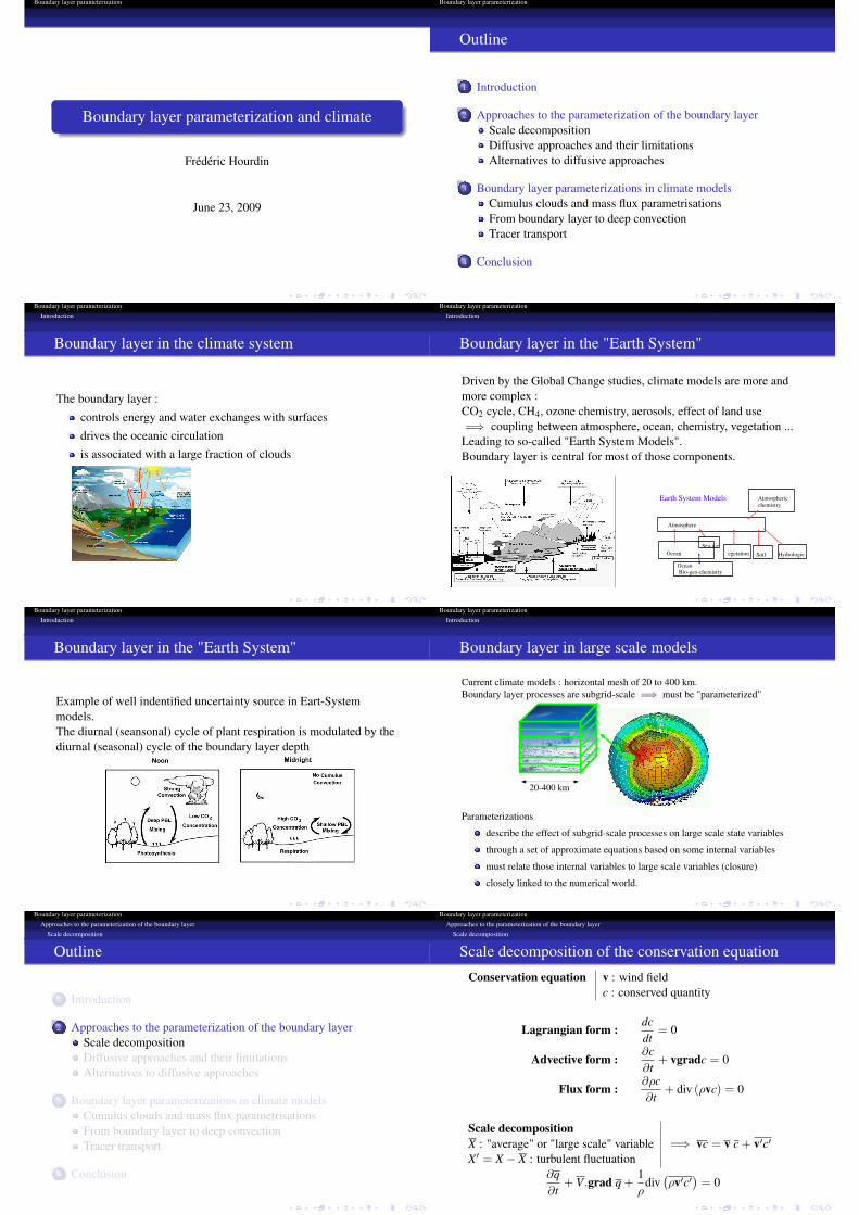
Scale decomposition of the conservation equation
Conservation equation v : wind fieldc : conserved quantity
Lagrangian form :dcdt
= 0
Advective form :∂c∂t
+ vgradc = 0
Flux form :∂ρc∂t
+ div (ρvc) = 0
Scale decompositionX : "average" or "large scale" variable =⇒ vc = v c + v′c′X′ = X − X : turbulent fluctuation
∂q∂t
+ V.grad q +1ρ
div(ρv′c′
)= 0
university-logo
Boundary layer parameterizationApproaches to the parameterization of the boundary layer
Scale decomposition
Under boundary layer approximations (∂/∂x << ∂/∂z) :
∂c∂t
+ v.grad c = Sc − 1ρ
∂
∂zw′c′
3D Dynamical core
200 km
20 km
One grid mesh or atmospheric column.
?Physical parametrizations
v and c are now the large scale variables.c : θ, u, v, water (vapor and others), chemical compounds ...
university-logo
Boundary layer parameterizationApproaches to the parameterization of the boundary layer
Diffusive approaches and their limitations
Outline
1 Introduction
2 Approaches to the parameterization of the boundary layerScale decompositionDiffusive approaches and their limitationsAlternatives to diffusive approaches
3 Boundary layer parameterizations in climate modelsCumulus clouds and mass flux parametrisationsFrom boundary layer to deep convectionTracer transport
4 Conclusion
university-logo
Boundary layer parameterizationApproaches to the parameterization of the boundary layer
Diffusive approaches and their limitations
Diffusive or local formulations for the PBL
w′c′ = −Kz∂c∂z
−→ ∂c∂t
=∂
∂z
(Kz∂c∂z
)
Analogy with molecular viscosity(Brownian motion↔ turbulence)
Down-gradient fluxes.
Turbulence acts as a "mixing"
university-logo
Boundary layer parameterizationApproaches to the parameterization of the boundary layer
Boundary layer parameterizationApproaches to the parameterization of the boundary layer
Alternatives to diffusive approaches
Outline
1 Introduction
2 Approaches to the parameterization of the boundary layerScale decompositionDiffusive approaches and their limitationsAlternatives to diffusive approaches
3 Boundary layer parameterizations in climate modelsCumulus clouds and mass flux parametrisationsFrom boundary layer to deep convectionTracer transport
4 Conclusionuniversity-logo
Boundary layer parameterizationApproaches to the parameterization of the boundary layer
Alternatives to diffusive approaches
Extension of diffusive formulations
Introduction of a countergradient term
w′θ′ = Kz
[Γ− ∂θ
∂z
]= 0 with Γ ' 1K/km (2)
Imposed countergradient Deardorf, 1966Revisited by Troen & Mart, 1986, Holtzlag & Boville, 1993,based on a similarity approach.
Non local mixing length (Bougeault)
Higher order closures- Mellor & Yamada 1974, hierarchy at successive orders.Complex and still local.- Abdella & Mc Farlane, 1997, Introduce a mass flux approach tocompute the 3rd order moments in a Mellor and Yamada scheme.
university-logo
Boundary layer parameterizationApproaches to the parameterization of the boundary layer
Alternatives to diffusive approaches
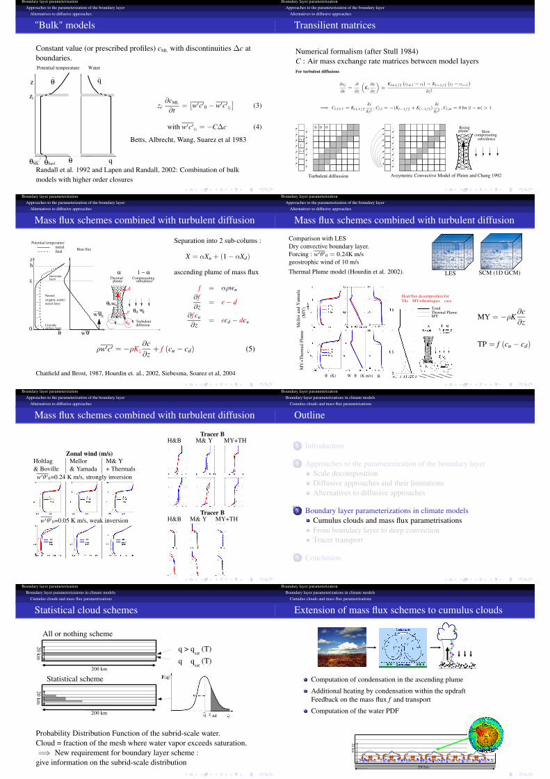
"Bulk" models
Constant value (or prescribed profiles) cML with discontinuities ∆c atboundaries.
θ
z
θ
θz q
qθ
Potential temperature Water
i
Surf.ML
zi∂cML
∂t=[w′c′
0 − w′c′zi
](3)
with w′c′zi = −C∆c (4)
Betts, Albrecht, Wang, Suarez et al 1983
Randall et al. 1992 and Lapen and Randall, 2002: Combination of bulkmodels with higher order closures university-logo
Boundary layer parameterizationApproaches to the parameterization of the boundary layer
Alternatives to diffusive approaches
Transilient matrices
Numerical formalism (after Stull 1984)C : Air mass exchange rate matrices between model layersFor turbulent diffusions
Boundary layer parameterizationBoundary layer parameterizations in climate models
Cumulus clouds and mass flux parametrisations
Outline
1 Introduction
2 Approaches to the parameterization of the boundary layerScale decompositionDiffusive approaches and their limitationsAlternatives to diffusive approaches
3 Boundary layer parameterizations in climate modelsCumulus clouds and mass flux parametrisationsFrom boundary layer to deep convectionTracer transport
4 Conclusion
university-logo
Boundary layer parameterizationBoundary layer parameterizations in climate models
Cumulus clouds and mass flux parametrisations
Statistical cloud schemes
200 km
20 km
q > qsat
(T)
q < qsat
(T)
All or nothing scheme
Statistical scheme
200 km
20 km
Probability Distribution Function of the subrid-scale water.Cloud = fraction of the mesh where water vapor exceeds saturation.=⇒ New requirement for boundary layer scheme :
give information on the subrid-scale distribution university-logo
Boundary layer parameterizationBoundary layer parameterizations in climate models
Cumulus clouds and mass flux parametrisations
Extension of mass flux schemes to cumulus clouds
αComputation of condensation in the ascending plume
Additional heating by condensation within the updraftFeedback on the mass flux f and transport
Computation of the water PDF
200 km
20 km
university-logo
Boundary layer parameterizationBoundary layer parameterizations in climate models
Cumulus clouds and mass flux parametrisations
1D test of the cloudy thermal plume model
Continental diurnal cycle with cumulusARM EUROCS case (US Oklahoma)Rio et al. 2008
LES SCM (1D GCM)
Turbulent diffusion
+ clouds - LES
+ mass flux
Specific humidity (g/kg)
Local time (h)
Cloud base height (m) Cloud top height (m)
Local time (h)
Local time (h)
Local time (h)
Cloud cover
university-logo
Boundary layer parameterizationBoundary layer parameterizations in climate models
Cumulus clouds and mass flux parametrisations
3D test of the cloudy thermal plume model
Test of the a new physical package in the LMDZ global climate modelImpact on the coverage by low clouds
university-logo
Boundary layer parameterizationBoundary layer parameterizations in climate models
Cumulus clouds and mass flux parametrisations
Cloud cover and satelite observations
9 et 10 février Visite du Comité d'experts 8
LowCloudscover
Calipso observations
LMDZ grid
LMDZ « newphysics »+ Calisposimulator
AtrainAtrain
university-logo
Boundary layer parameterizationBoundary layer parameterizations in climate models
From boundary layer to deep convection
Outline
1 Introduction
2 Approaches to the parameterization of the boundary layerScale decompositionDiffusive approaches and their limitationsAlternatives to diffusive approaches
3 Boundary layer parameterizations in climate modelsCumulus clouds and mass flux parametrisationsFrom boundary layer to deep convectionTracer transport
4 Conclusion
university-logo
Boundary layer parameterizationBoundary layer parameterizations in climate models
From boundary layer to deep convection
Parameterization of deep convection
Classical parameterizations :Mass flux schemes
Importance of cloud phase changes and rainfall
Controled by instability above cloud baseExample of the Emanuel (1991) scheme :
Boundary layer parameterizationBoundary layer parameterizations in climate models
From boundary layer to deep convection
A systematic biais of parameterized convection
Climate models with parameterized convection tend to predictcontinental convection in phase with insolation, while it peaks in lateafternoon in reality and in Cloud Resolving Models (mesh ' 1 km).
An idealized case of continental cycle with deep convectionARM, Oklahoma, after Guichard et al. 2004
CRMs
SCMs
Deep convection preceeded by a phase of shallow cumulus convection
Boundary layer : preconditioning and trigerring of deep convection
university-logo
Boundary layer parameterizationBoundary layer parameterizations in climate models
From boundary layer to deep convection
ARM case with the standard LMD SCM
CRMsLMDz standard
15 181296h
100m
1km
10km
Local time (h)
z
Mellor & Yamada
Emanuel (1991)
university-logo
Boundary layer parameterizationBoundary layer parameterizations in climate models
From boundary layer to deep convection
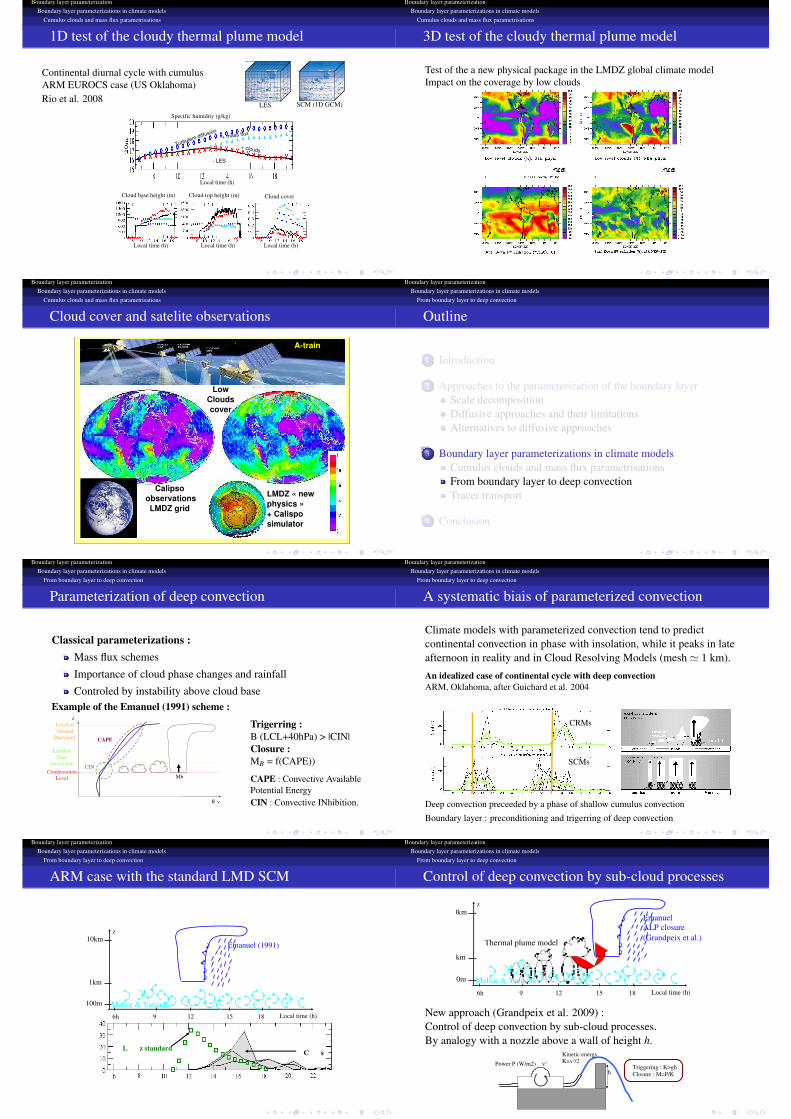
Control of deep convection by sub-cloud processes
15 181296h
100m
1km
10km
Local time (h)
z
Mellor & Yamada
Thermal plume model
EmanuelALP closure(Grandpeix et al.)
New approach (Grandpeix et al. 2009) :Control of deep convection by sub-cloud processes.By analogy with a nozzle above a wall of height h.
Power P (W/m2) ~ v3
Kinetic energyK=v2/2
hTriggering : K>ghClosure : M=P/K
university-logo
Boundary layer parameterizationBoundary layer parameterizations in climate models
From boundary layer to deep convection
ALP closure
Avaliable Lifting Energy for the convectionScaling with w2.Trigerring : ALE > |CIN|
Avaliable Lifting Power for the convectionScaling with w3.Closure : MB = f (ALP)
New requirements for the boundary layer scheme :give reasonable estimates of w′2 and w′3.
university-logo
Boundary layer parameterizationBoundary layer parameterizations in climate models
From boundary layer to deep convection
Statistical cloud schemes
WakeDensity currentsCold pool
Gust front
liftingPrecipitatingdowndraughts
Newconvection
Matureconvection
university-logo
Boundary layer parameterizationBoundary layer parameterizations in climate models
From boundary layer to deep convection
ARM case with ALP closure, thermals and wakes
15 181296h
100m
1km
10km
Local time (h)
z
Mellor & Yamada
Thermal plume model
EmanuelALP closure(Grandpeix et al.)
New physics
Rio & al., GRL, 2008
CRMsLMDz standardversion
university-logo
Boundary layer parameterizationBoundary layer parameterizations in climate models
From boundary layer to deep convection
ARM case with ALP closure, thermals and wakes
Convective heating rate (K/day)
heure locale heure locale
Pressure (hPa)Pressure ( hPa)
CRM/MesoNH
LMDZ, old physics Emanuel + MY + thermal plume
Ema. + MY + Therm. + wakes
university-logo
Boundary layer parameterizationBoundary layer parameterizations in climate models
From boundary layer to deep convection
Diurnal cycle of deep convection in the 3D LMDZ GCM
200 km
20 km
3D testDiurnal cycleOf rainfall overSenegal(Sept. 2006, AMMA)Raingaugenetwork
LMDZ New physical package
university-logo
Boundary layer parameterizationBoundary layer parameterizations in climate models
Tracer transport
Outline
1 Introduction
2 Approaches to the parameterization of the boundary layerScale decompositionDiffusive approaches and their limitationsAlternatives to diffusive approaches
3 Boundary layer parameterizations in climate modelsCumulus clouds and mass flux parametrisationsFrom boundary layer to deep convectionTracer transport
4 Conclusion
university-logo
Boundary layer parameterizationBoundary layer parameterizations in climate models
Tracer transport
Boundary layer and transport of atmospheric tracers
Test of 222Rn transport : emitted on conitnents only
Test with various parameterizations of the planetary boundary layer
(may) days of year (june)(may) days of year (june)
* Radon is a tracer of continental air masses, emited almost uniformely by continents only. Life time of about 4 days.
(may) days of year (june)
Zingst
Heidelberg
Mace Head
university-logo
Boundary layer parameterizationBoundary layer parameterizations in climate models
Tracer transport
Boundary layer and transport of atmospheric tracers
Contribution of the biosphere to the CO2 latitudinal contrasts
Idealized seasonal cycle for surface emission (null annual mean)GCM and transport models from the Transcom exercizeAfter Dargaville et al.
university-logo
Boundary layer parameterizationBoundary layer parameterizations in climate models
Tracer transport
Boundary layer and transport of atmospheric tracers
NOX computation at Dome C, AntarticaMAR Regional model
university-logo
Boundary layer parameterizationConclusion
Concluding remarks
Parameterization of boundary layer processes is a key issue for climatemodeling and climate change studies.
Climate models are more and more complex but the realism of the "newcomponents" (chemistry, vegetation, ...) highly depends on the representationof atmospheric processes in general and boundary layer in particular.
In current climate models (and still for a while), boundary layer processes mustbe parameterized.
Boundary layer schemes must be valid from equator to pole, and from drystable atmosphere to deep convection conditions.
The "new components" put new constraints on boundary layer schemes.
There is a large place for improvement of boundary layer parameterization.
The combined use of a turbulent diffusion for small scales and mass fluxschemes for organized structures seems a promizing way.
A hierarchy of approaches are available to improve and evaluate boundarylayer parameterizations : 1D versus LES , 3D, nudged, weather forecast andclimate, etc.