Abstract We establish sufficient conditions for a cohomology class of a discrete sub-group � of a connected semisimple Lie group with finite center to be representableby a bounded differential form on the quotient by � of the associated symmetricspace; furthermore if ρ : � → PU(1, q) is any representation of any discrete sub-group � of SU (1, p), we give an explicit closed bounded differential form on thequotient by � of complex hyperbolic space which is a representative for the pullbackvia ρ of the Kähler class of PU(1, q). If G, G′ are Lie groups of Hermitian type, wegeneralize to representations ρ : � → G′ of lattices � < G the invariant definedin [Burger, M., Iozzi, A.: Bounded cohomology and representation variates in PU(1, n). Preprint announcement, April 2000] for which we establish a Milnor–Woodtype inequality. As an application we study maximal representations into PU(1, q) oflattices in SU(1, 1).
Alessandra Iozzi was partially supported by FNS grant PP002-102765.
M. BurgerFIM, ETH Zentrum, Rämistrasse 101, CH-8092 Zürich, Switzerlande-mail: [email protected]
A. Iozzi (B)Institut für Mathematik, Universität Basel, Rheinsprungstrasse 21, CH-4051 Basel, Switzerlande-mail: [email protected]
Départment de Mathématiques, Université de Strasbourg, 7, Rue René Descartes, F-67084Strasbourg Cedex, France ·Permanent Address:Department of Mathematics, ETH Zentrum, Raemistrasse 101, CH-8092 Zuerich, Switzerland
2 Geom Dedicata (2007) 125:1–23
1. Introduction
The continuous cohomology H•c(G, R) of a topological group G is the cohomology
of the complex(C(G•)G, d•) of G-invariant continuous functions, while its bounded
continuous cohomology H•cb(G, R) is the cohomology of the subcomplex (Cb(G•)G, d•)
of G-invariant bounded continuous functions. The inclusion of the complex of boundedcontinuous functions into the one consisting of continuous functions gives rise to thecomparison map
c•G: H•
cb(G, R) → H•c(G, R)
which encodes subtle properties of G of algebraic and geometric nature, see [1,12,19,20, Section V.13, 29,44,45] (see also [2,3,7,8,26–28,35,39,40,49] in relation with theexistence of quasi-morphisms). We say that a continuous class on G is representableby a bounded continuous class if it is in the image of c•
G.When G is a connected semisimple Lie group with finite center and associated
symmetric space X and L < G is any closed subgroup, a useful tool in the studyof the continuous cohomology of L is the van Est isomorphism, according to whichH•
c(L, R) is canonically isomorphic to the cohomology H•(�•(X )L)
of the complex(�•(X )L, d•) of L-invariant smooth differential forms �•(X ) on X . For example,
if � < G is a torsionfree discrete subgroup, H•(�, R) is the de Rham cohomologyH•
dR(�\X ) of the manifold �\X . (Here and in the sequel we drop the subscript c ifthe group is discrete.) For simplicity, in the introduction we restrict ourselves to thiscase, and we refer the reader to the body of the paper for the general statement in thecase in which � is an arbitrary closed subgroup.
We do not know of an analogue of van Est theorem in the context of continuousbounded cohomology. This paper however explores a particular aspect of the com-parison map and of the pullback, namely the relation between bounded continuouscohomology and the complex of, loosely speaking, invariant smooth differential formswith some boundedness condition. For instance, our first result gives us informationon the differential forms that one can use to represent a class in the image of thecomparison map.
Theorem 1 Let � < G be a torsionfree discrete subgroup of a connected semisimpleLie group G with finite center and associated symmetric space X . Any class in the imageof the comparison map
c•�: H•
b(�, R) → H•(�, R) ∼= H•dR(�\X )
is representable by a closed form on �\X which is bounded.
Here a form is bounded on �\X if its supremum norm, computed using the Rie-mannian metric, is finite. In fact, this is only a particular case of the following moregeneral result which describes some of the interplay between the comparison mapand the pullback of a cohomology class via a homomorphism of a discrete group intoa topological group (which in the case of Theorem 1 is the identity homomorphism).
Theorem 2 Let � < G be a torsionfree discrete subgroup of a connected semisimpleLie group G with finite center and associated symmetric space X , and ρ : � → G′a homomorphism into a topological group G′. If α ∈ Hn
c (G′, R) is representable bya continuous bounded class, then its pullback ρ(n)(α) ∈ Hn(�, R) ∼= Hn
dR(�\X ) isrepresentable by a closed differential n-form on �\X which is bounded.
Geom Dedicata (2007) 125:1–23 3
We shall see later that in the case in which G, G′ are the connected componentsof the isometry groups of complex hyperbolic spaces and α is the Kähler class, thebounded closed 2-form in Theorem 2 can be given explicitly (see Theorem 5).
Even if G′ is a connected Lie group, little is known about the surjectivity propertiesof the comparison map c•
G′ . However, as a direct consequence of a theorem of Gro-mov [36] which asserts that characteristic classes are bounded (see [9] for a resolutionof singularities free proof), we have the following:
Corollary 3 Let � < G be a torsionfree discrete subgroup of a connected semisimpleLie group with finite center G and associated symmetric space X , and let ρ : � → G′be a homomorphism into a real algebraic group G′. If α ∈ Hn
c (G′, R) comes from acharacteristic class of a flat principal G′-bundle, then its pullback ρ(n)(α) ∈ Hn(�, R) ∼=Hn
dR(�\X ) is representable by a closed differential n-form on �\X which is bounded.
Notice that Theorem 1, and hence Theorem 2 and Corollary 3 are valid, with anappropriate formulation, for any closed subgroup � < G (compare with Corollary 4.1and Proposition 3.1).
Moreover, as a consequence of the surjectivity of the comparison map for Gromovhyperbolic groups [36,44,45] we have immediately:
Corollary 4 Let � < G be a torsionfree discrete subgroup of a connected semisimpleLie group with finite center G and associated symmetric space X . Assume that � isfinitely generated and word hyperbolic. Then for every n ≥ 2, any class in Hn
dR(�\X )
is representable by a closed differential n-form on �\X which is bounded.
If L is a connected semisimple group with finite center, one has full informationabout the comparison map in degree two,
c(2)L : H2
cb(L, R) → H2c(L, R) (1.1)
which is an isomorphism1 [20]. This is the case we exploit, also because in this degreecontinuous cohomology is connected to a particularly fundamental geometric struc-ture. Recall in fact that if Y is the symmetric space associated to L, the dimension ofH2
c(L, R) is the number of irreducible factors of Y which are Hermitian symmetric and�2(Y)L is generated by the Kähler forms of the irreducible Hermitian factors of Y . Wesay that a connected semisimple Lie group L with finite center is of Hermitian type2 ifY is Hermitian symmetric; we denote by ωY the Kähler form on Y , by κY ∈ H2
c(L, R)
the corresponding continuous class under the isomorphism H2(�•(Y)L) ∼= H2
c(L, R)
and by κbY ∈ H2
cb(G, R) its image under the isomorphism (1.1).In the particular case of the complex hyperbolic spaces H�
C, we can give explicitly
the expression of the representative in Theorem 2. In fact in this case the multiple1πκb� of the bounded Kähler class κb
� (which is here and in the following a shortcut forκb
H�C
) admits an explicit representative on ∂H�C
given by the Cartan cocycle
c�: (∂H�C)3 → [−1, 1],
1 A similar statement holds, again in degree two, for any connected Lie group.2 In [16] a group of Hermitian type is required not to have compact factors, but this assumption is notnecessary here.
4 Geom Dedicata (2007) 125:1–23
(see Sect. 6 for the definition and properties). Moreover, if x ∈ HpC
and ξ is a pointin the boundary ∂Hp
Cof complex hyperbolic space, let eξ (x) := ehβξ (0,x), where h is
the volume entropy of HpC
, βξ (0, x) is the Busemann function relative to a basepoint0 ∈ Hp
C, and µ0 the K = StabSU(1,p)(0)-invariant probability measure on ∂Hp
C. Then
we have:
Theorem 5 Let � < SU(1, p) be any torsionfree discrete subgroup, and let ρ : � →PU(1, q) be a homomorphism with nonelementary image and associated �-equivariantmeasurable map ϕ: ∂Hp
C→ ∂Hq
C. The 2-form
∫
(∂HpC
)3eξ0 ∧ deξ1 ∧ deξ2 cq
(ϕ(ξ0), ϕ(ξ1), ϕ(ξ2)
)dµ0(ξ0)dµ0(ξ1)dµ0(ξ2)
is �-invariant, closed, bounded and represents 1πρ(2)(κq) ∈ H2
dR(�\HpC).
As an application of the above results, we prove here a generalization of the Mil-nor–Wood inequality. Namely, to any representation of a torsionfree lattice � < G intoG′, where G, G′ are of Hermitian type, we associate a numerical invariant which wethen prove to be bounded with a bound depending only on the rank of the symmetricspaces.
To define the aforementioned invariant, let G be of Hermitian type with associ-ated symmetric space X and � < G a torsionfree lattice; for 1 ≤ p ≤ ∞ let H•
p(�\X )
denote the Lp-cohomology of �\X , which is the cohomology of the complex of smoothdifferential forms α on �\X such that α and dα are in Lp. Inclusion in the complex ofsmooth differential forms gives thus a comparison map
i•p: H•p(�\X ) → H•
dR(�\X ) .
Then we have:
Corollary 6 Assume that G, G′ are of Hermitian type, let � < G be a torsionfree lattice,X the Hermitian symmetric space associated to G and ρ: � → G′ a homomorphism.Then for every 1 ≤ p ≤ ∞ there is a linear map
ρ(2)p : H2
c(G′, R) → H2
p(�\X )
such that the diagram
H2c(G
′, R)
ρ(2)p ������������
ρ(2)
�� H2(�, R)∼= �� H2
dR(�\X )
H2p(�\X )
i(2)p
���������������������
commutes.
In the above situation—that is if � < G is a lattice and X is Hermitian symmetric—the L2-cohomology H•
2(�\X ) is reduced (i.e. Hausdorff) and finite dimensional in alldegrees; it may hence be identified with the space of L2-harmonic forms on �\X andcarries a natural scalar product 〈 · , · 〉. The Kähler form ω�\X is thus a distinguished
Geom Dedicata (2007) 125:1–23 5
element of H22(�\X ). Given now a homomorphism ρ: � → G′ and using Corollary 6,
the invariant
iρ :=⟨ρ
(2)2 (κX ′), ω�\X
⟩
⟨ω�\X , ω�\X
⟩ (1.2)
is well defined and finite. We have then finally the Milnor–Wood type inequality:
Theorem 7 Let G, G′ be of Hermitian type with associated symmetric spaces X and X ′,let ρ: � → G′ be a representation of a lattice in G with invariant iρ as in (1.2). Assumethat X is irreducible and that the Hermitian metrics on X and X ′ are normalized so asto have minimal holomorphic sectional curvature −1. Then
|iρ | ≤ rk X ′
rk X . (1.3)
Special cases of the above theorem for invariants related to ours had been previ-ously obtained, with restrictions on the target group and cocompactness conditions,by Milnor [43], Wood [52], Turaev [51], Toledo [50], Bradlow et al. [6] and Koziarzand Maubon [41]. In particular, if � is a torsionfree lattice in PU(1, 1) so that �\X isdiffeomorphic to the interior of a compact oriented surface �, then iρ is, up to themultiple χ(�), equal to the Toledo invariant defined in [16,Section 1]: notice howeverthat this equality implies that iρ is independent of the hyperbolization on the interiorof � [16].
The study of maximal representations, that is representations such that the invari-ant iρ takes its maximum value rk X ′/rk X , has been the subject of much researchover the years [6,14–18,23,29–32,34,38,41,42]. If � < G is cocompact, then iρ is acharacteristic number. If G is of rank one, that is if it is locally isomorphic to SU(1, p),then if p ≥ 2, H2
2(�\HpC) injects into H2
dR(�\HpC) [48,54], and hence once again iρ is
a characteristic number. When G is locally isomorphic to SU(1, 1) and � < G is notcocompact, then H2
2(�\H1C) is one-dimensional while H2
dR(�\H1C) = 0; this case has
a different flavor as iρ is not a characteristic number, a fact which is reflected by theexistence of nontrivial deformations of � in PU(1, 2) [37].
For the rest of the paper we focus our attention to the case in which G is locallyisomorphic to SU(1, 1) and � < G is any lattice.
Theorem 8 ([10]) Let � < G be a lattice in a connected group locally isomorphic toSU(1, 1) and let ρ : � → PU(1, q) be a representation such that |iρ | = 1. Then ρ(�)
leaves a complex geodesic invariant.
This was proven by Toledo [50] if � is a compact surface group. In the noncompactcase a variant of Theorem 8 was obtained by Koziarz and Maubon [41], with anotherdefinition of maximality which probably coincides with ours.
Thus Theorem 8 reduces the study of maximal representations into PU(1, q) to thecase q = 1, for which we have the following:
Theorem 9 ([10]) Let � < G be a lattice, where G = SU(1, 1) or G = PU(1, 1) and letρ: � → PU(1, 1) be a maximal representation. Then ρ(�) is discrete and, modulo thecenter of �, ρ is injective. In fact, there is a continuous surjective map f : ∂H1
C→ ∂H1
C
such that:
6 Geom Dedicata (2007) 125:1–23
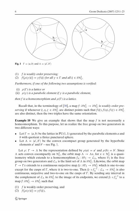
a
b
a
b
Fig. 1 � = 〈a, b〉 and � = 〈a′, b′〉
(1) f is weakly order preserving;(2) f
(ρ(γ )ξ
) = γ f (ξ) for all γ ∈ � and all ξ ∈ ∂H1C
.
Furthermore, if one of the following two assumptions is verified:
(i) ρ(�) is a lattice or(ii) ρ(γ ) is a parabolic element if γ is a parabolic element,
then f is a homeomorphism and ρ(�) is a lattice.
Recall that, in the terminology of [38], a map f : ∂H1C
→ ∂H1C
is weakly order pre-serving if whenever ξ , η, ζ ∈ ∂H1
Care distinct points such that f (ξ), f (η), f (ζ ) ∈ ∂H1
C
are also distinct, then the two triples have the same orientation.
Example 10 We give an example that shows that the map f is not necessarily ahomeomorphism. To this purpose, let us realize the free group on two generators intwo different ways:
• Let � = 〈a, b〉 be the lattice in PU(1, 1) generated by the parabolic elements a andb with quotient a thrice punctured sphere.
• Let � = 〈a′, b′〉 be the convex cocompact group generated by the hyperbolicelements a′ and b′—see Fig. 1.
Let ρ : � → � be the representation defined by ρ(a) = a′ and ρ(b) = b′. Since� acts convex cocompactly on H1
C, the orbit map � → �x, for x ∈ H1
Cis a quasi-
isometry which extends to a homeomorphism f� : ∂F2 → L�, where F2 is the freegroup on two generators and L� is the limit set of � in ∂H1
C. Likewise, the orbit map
� → �x extends to a continuous surjective map f�: ∂F2 → ∂H1C
which is one-to-oneexcept for the cusps of �, where it is two-to-one. Then f� ◦ f −1
� : L� → ∂H1C
is alsocontinuous, surjective and two-to-one on the cusps of �. By sending any interval inthe complement of L� in ∂H1
Cto the image of its endpoints, we extend f� ◦ f −1
� to amap f: ∂H1
C→ ∂H1
Csuch that
(1) f is weakly order preserving, and(2) f
(ρ(γ )ξ
) = γ f (ξ),
Geom Dedicata (2007) 125:1–23 7
One can prove, using the results in [29], Sects. 2.1 and 5 that iρ = 1 (see Remark 5.4).
Finally we conclude with the following:
Corollary 11 Any maximal representation ρ : � → PU(1, 1) of a torsionfree lattice� < PU(1, 1) is induced by a diffeomorphism
�\H1C
→ ρ(�)\H1C
. (1.4)
Organization of the Paper: Theorem 1 is proven as Proposition 3.1, Theorem 2 isproven as Corollary 4.1, Theorem 5 is Proposition 6.2 Corollary 6 is proven as Corol-lary 4.2, Theorem 7 follows from Lemma 5.1 and Lemma 5.3, and Theorems 8 and 9and Corollary 11 are proven in Sect. 6.
2. Preliminaries on bounded cohomology, old and new: the Toledo map and thebounded Toledo map
Let G be a locally compact group. The continuous bounded cohomology of G (withtrivial coefficients) is the cohomology of the complex
(Cb(G•)G, d•) of the space of
continuous bounded functions Gn+1 → R which are G-invariant with respect to thediagonal G-action on Gn+1. Notice that H•
cb(G, R) comes naturally equipped with aseminorm induced by the supremum norm on Cb(G•, R) and in some cases, as forinstance in degree two, the seminorm is actually a norm.
Analogously to the case of the continuous cohomology, there are notions of rel-atively injective G-module and of strong resolution which serve for the homologicalalgebra characterization of bounded continuous cohomology. For the precise defini-tions see [20,46], while for our purpose it will suffice to say that if (S, ν) is a regularmeasure G-space, then the G-module L∞
alt(S) of L∞ alternating functions on S is rel-atively injective if and only if the G-action on S is amenable in the sense of Zimmer[53]. Moreover
(L∞
alt(S•), d•) is a strong resolution of R and hence the cohomology of
the subcomplex of G-invariants
0 ��L∞alt(S)G ��L∞
alt(S2)G �� · · · ��L∞
alt(Sn)G dn �� · · · ,
is canonically isomorphic to the bounded continuous cohomology of G.
2.1. The transfer map in bounded continuous and continuous cohomology
Let G be a locally compact second countable group and L < G a closed subgroup.The injection L ↪→ G gives by contravariance the restriction map
r•: H•cb(G, R) → H•
cb(L, R)
in bounded cohomology. If we assume that L\G has a G-invariant probability measureµ, then the transfer map
T•: Cb(G•)L → Cb(G•)G ,
defined by integration
T(n)f (g1, . . . , gn) :=∫
L\Gf (gg1, . . . , ggn)dµ(g) , (2.1)
8 Geom Dedicata (2007) 125:1–23
for all (g1, . . . , gn) ∈ Gn, induces in cohomology a left inverse of r• of norm one
T•b : H•
cb(L, R) → H•cb(G, R) ,
(see [46, Proposition 8.6.2, pp. 106–107]).Notice that an analogous construction in continuous cohomology fails in the case in
which L\G carries a G-invariant probability measure µ but is not compact. For exam-ple, if L = � < G is a nonuniform lattice, then there is in general no left inverse tothe restriction in cohomology H•
c(G, R) → H•(�, R) as this map is often not injective.In fact, one can for instance consider the case in which X = G/K is an n-dimensionalsymmetric space of noncompact type: then Hn
c (G, R) = �n(X )G is generated by thevolume form and hence not zero, while if � < G is any nonuniform torsionfree lattice,the cohomology Hn(�, R) vanishes as it is isomorphic to Hn
dR(�\X ).However, if L\G carries a finite invariant measure and is compact we can indeed
define a transfer map in continuous cohomology. In fact, under these hypotheses,there is an obvious morphism of coefficient modules
m: Lp(L\G) → R
f �→∫
L\Gf dµ ,
and moreover, since L\G is compact, then Lploc(L\G) = Lp(L\G); one can hence
compose the general induction map [4] valid for any closed subgroup
ı•: H•c(L, R) → H•
c(G, Lp
loc(L\G))
with the change of coefficients m in ordinary continuous cohomology to obtain atransfer map which is a left inverse to the restriction map and leads to a commutativediagram
H•cb(L, R)
T•b
��
c•L �� H•
c(L, R)
T•��
H•cb(G, R)
c•G �� H•
c(G, R)
(2.2)
which is very useful in applications when it comes to identifying invariants in boundedcohomology in terms of ordinary cohomological invariants.
Before passing to the next subsection, we record here for later use that—althoughnot really functorial since defined only on the subcomplex of L-invariants—the trans-fer map in continuous bounded cohomology can also be implemented on the com-plex of L∞ alternating L-invariant functions on an amenable L-space. In fact [46,Proposition 10.1.3] implies the following:
Lemma 2.1 Let L < G be a closed subgroup of a locally compact group G, and let(S, ν) be a regular amenable G-space. Let
T•S:
(L∞
alt
(S•)L, d•) → (
L∞alt
(S•)G, d•) (2.3)
be defined by
T(n)S f (x1, . . . , xn) :=
∫
L\Gf (gx1, . . . , gxn)dµ(g) , (2.4)
Geom Dedicata (2007) 125:1–23 9
for (x1, . . . , xn) ∈ Sn, and let
T•S,b: H•
cb(L, R) → H•cb(G, R)
be the map obtained by the composition
H•(L∞alt(S
•)L, d•) ��
∼=��
H•(L∞alt(S
•)G, d•)
∼=��
H•cb(L, R)
T•S,b �� H•
cb(G, R) ,
(2.5)
where the vertical arrows are the canonical isomorphisms in bounded cohomologyextending the identity R → R, and the top horizontal arrow is the map in cohomologyinduced by T•
S in (2.3).Then T•
S,b = T•b.
2.2. The Toledo map and the bounded Toledo map
Let L ≤ G be a closed subgroup of a locally compact second countable group Gsuch that on L\G there is a G-invariant probability measure, and let ρ: L → G′ be acontinuous homomorphism into a locally compact group G′. The composition of thepullback
ρ•b: H•
cb(G′, R) → H•cb(L, R)
with the transfer map T•b defined in (2.1) gives rise to the bounded Toledo map
T•b(ρ): H•
cb(G′, R) → H•cb(G, R) (2.6)
which is the source of basic invariants of the homomorphism ρ: L → G′.A good part of this paper will be devoted to the interpretation and properties of a
numerical invariant defined by this map in the case in which the cohomology spacesinvolved are one-dimensional (see Sect. 5). To this purpose, remark that if L\G isin addition compact (for example, a uniform lattice) then we also have an analo-gous construction in ordinary cohomology. Namely, associated to the homomorphismρ: L → G′ we have the pullback
ρ•: H•c(G
′, R) → H•c(L, R)
which, composed with the transfer map T• defined above gives a map
T•(ρ): H•c(G
′, R) → H•c(G, R)
which we call the Toledo map and which has the property that the diagram
H•cb(G′, R)
T•b(ρ)
��
c•G′ �� H•
c(G′, R)
T•(ρ)
��H•
cb(G, R)c•
G �� H•c(G, R) ,
where the horizontal arrows are comparison maps, commutes.The interplay between these two maps is the basic ingredient in the interpretation
of the above invariants in this paper for the cocompact case, as well as in [16–18,38].
10 Geom Dedicata (2007) 125:1–23
In the finite volume case we will need to resort to a somewhat more elaborate versionof the above diagram which can be developed when G is a connected semisimple Liegroup—see (5.5) and which will encompass the above description.
3. A factorization of the comparison map
The main point of this section is to provide, in the case of semisimple Lie groups, asubstitute to the the missing arrow in
H•cb(L, R)
T•b
��
c•L �� H•
c(L, R)
��H•
cb(G, R)c•
G �� H•c(G, R)
(3.1)
if the subgroup L ≤ G is only of finite covolume.Let G be a connected semisimple Lie group with finite center and X the associated
symmetric space. Any closed subgroup L ≤ G acts properly on X and hence thecomplex
R ���0(X ) �� · · · ���k(X ) �� · · ·of C∞ differential forms on X with the usual exterior differential is a resolution bycontinuous injective L-modules (where injectivity now refers to the usual notion incontinuous cohomology), from which one obtains a canonical isomorphism
H•(�•(X )L) ∼= ��H•
c(L, R)
in cohomology [47]. Let moreover(�•∞(X ), d•) denote the complex of smooth differ-
ential forms α on X such that the functions x �→ ‖αx‖ and x �→ ‖dαx‖ are in L∞(X ),and let h(X ) denote the volume entropy of X , that is the rate of exponential growthof volume of geodesic balls in X [25]. Then we have:
Proposition 3.1 Let G be a connected semisimple Lie group with finite center, X theassociated symmetric space and let L ≤ G be any closed subgroup. Then there exists amap
δ•∞,L: H•
cb(L, R) → H•(�•∞(X )L)
such that the diagram
H•cb(L, R)
c•L ��
δ•∞,L ����������������H•
c(L, R) H•(�•(X )L)∼=��
H•(�•∞(X )L)
i•∞,L
�������������
(3.2)
commutes, where i•∞,L is the map induced in cohomology by the inclusion of complexes
i•∞: �•∞(X ) → �•(X ) .
Moreover, the norm of δ(k)∞,L is bounded by h(X )k.
Geom Dedicata (2007) 125:1–23 11
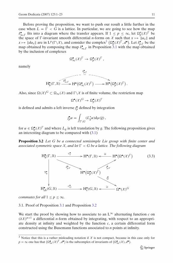
Before proving the proposition, we want to push our result a little further in thecase when L = � < G is a lattice. In particular, we are going to see how the mapδ•∞,� fits into a diagram where the transfer appears. If 1 ≤ p ≤ ∞, let �n
p(X )� bethe space of �-invariant smooth differential n-forms on X such that x �→ ‖αx‖ andx �→ ‖dαx‖ are in Lp(�\X ), and consider the complex3 (
�•p(X )� , d•). Let δ•
p,� be themap obtained by composing the map δ•∞,� in Proposition 3.1 with the map obtainedby the inclusion of complexes
�•∞(X )� → �•p(X )� ,
namely
H•b(�, R)
δ•∞,� ��
δ•p,�
��H•(�•∞(X )�
) �� H•(�•p(X )�
).
Also, since �(X )G ⊂ �∞(X ) and �\X is of finite volume, the restriction map
�•(X )G → �•p(X )�
is defined and admits a left inverse j•p defined by integration
j•pα =∫
�\G(L∗
gα)dµ(g) ,
for α ∈ �•p(X )� and where Lg is left translation by g. The following proposition gives
an interesting diagram to be compared with (3.1)
Proposition 3.2 Let G be a connected semisimple Lie group with finite center andassociated symmetric space X , and let � < G be a lattice. The following diagram
H•b(�, R)
T•b
��
c•� ��
δ•p,� ����������������
H•(�, R) H•(�•(X )�)∼=��
H•(�•p(X )�
)i•p,�
�������������
j•p
�������������
H•cb(G, R)
c•G �� H•
c(G, R) �•(X )G∼=��
(3.3)
commutes for all 1 ≤ p ≤ ∞.
3.1. Proof of Proposition 3.1 and Proposition 3.2
We start the proof by showing how to associate to an L∞ alternating function c on(∂X )n+1 a differential n-form obtained by integrating, with respect to an appropri-ate density at infinity and weighted by the function c, a certain differential formconstructed using the Busemann functions associated to n points at infinity.
3 Notice that this is a rather misleading notation if X is not compact, because in this case only forp = ∞ one has that
(�•∞(X )� , d•)
is the subcomplex of invariants of(�•∞(X ), d•)
.
12 Geom Dedicata (2007) 125:1–23
So, let us consider on X the Riemannian metric obtained from the Killing form andlet
B: ∂X × X × X → R
be the Busemann cocycle, where ∂X is the geodesic ray boundary of X . Fix a basepoint0 ∈ X and let K = StabG(0), g = k ⊕ p the associated Cartan decomposition, a+ ⊂ p
a positive Weyl chamber and b ∈ a+ the vector predual to the sum of the positive rootsassociated to a+. Then h(X ) = ‖b‖. Let ξb ∈ ∂X be the point at infinity determinedby b; let ν0 be the unique K-invariant probability measure on Gξb ⊂ ∂X . Then
d(g∗ν0)(ξ) = e−h(X )Bξ (g0,0)dν0(ξ) . (3.4)
For ξ ∈ ∂X , let us define a C∞ map by
eξ : X −→ R
x �→ e−h(X )Bξ (x,0).(3.5)
Lemma 3.3 Let G be a connected semisimple Lie group with finite center, and letX be its associated symmetric space with geodesic ray boundary ∂X . For each c ∈L∞
Proof For ξ ∈ ∂X , let Xξ (x) be the unit tangent vector at x pointing in the direc-tion of ξ , and let gx( · , · ) be the Riemannian metric on X at x. Since the gradientof the Busemann function Bξ (x, 0) at x is −Xξ (x) [25], we have that for v ∈ (TX )x,(dBξ )x(v) = −gx
(v, Xξ (v)
).
Then(deξ )x(v) = h(X )gx
(v, Xξ (x)
)eξ (x) .
This implies that if v1, . . . , vn are tangent vectors based at x, then
|ωx(v1, . . . , vn)|≤ h(X )n
∫
(∂X )n+1
∣∣c(ξ0, ξ1, . . . , ξn)∣∣eξ0(x)
×(
n∏
i=1
∣∣gx(vi, Xξi(x)
)∣∣ eξi(x)
)
dνn+10 (ξ0, . . . , ξn)
≤ h(X )n‖c‖∞(∫
∂Xeξ0(x)dν0(ξ0)
) n∏
i=1
(‖vi‖
∫
∂Xeξi(x)dν0(ξi)
),
Geom Dedicata (2007) 125:1–23 13
where we used that∣∣gx
(vi, Xξi(x)
)∣∣ ≤ ‖vi‖. But writing x = g0 and using that, as indi-cated in (3.4), d(g∗ν0) is a probability measure, we get from (3.4) that for all 0 ≤ i ≤ nand all x ∈ X ∫
∂Xeξi(x)dν0(ξi) = 1 , (3.8)
which shows that
|ωx(v1, . . . , vn)| ≤ h(X )n‖c‖∞n∏
i=1
‖vi‖ ,
so that ifδ•∞: L∞
alt
((∂X )• + 1, ν• + 1
0
) → �•(X ) ,
we have that
‖δ(n)∞ c‖ = supx∈X
sup‖v1‖,...,‖vn‖≤1
|ωx(v1, . . . , vn)| ≤ h(X )n‖c‖∞ .
This proves (3.7) and the fact that the image δ(n)∞ (c) is a bounded form. Once we shall
have proven that δ(n)∞ (dc) = dδ
(n−1)∞ (c), it will follow automatically that also dδn−1∞ (c)is bounded and hence the image of δ•∞ is in �•∞(X ). To this purpose, let us computefor c ∈ L∞
The G-equivariance of δ•∞ follows from (3.4) and the cocycle property of theBusemann function Bξ (x, y), hence completing the proof. �
Proof of Proposition 3.1 This is a direct application of [46, Proposition 9.2.3]. Indeed,since the L-action on (∂X , ν0) is amenable, we have that
(L∞
alt
((∂X )• + 1, ν• + 1
0
))is
a strong resolution of R by relatively injective L-modules [20]; moreover, it is wellknown that, (�•(X ), d•) is a resolution of R by injective continuous L-modules, wherein this case injectivity is meant in ordinary cohomology (see [47]), and �•(X ) is asusual equipped with the C∞-topology. Finally one checks on the formulas that thecomposition i•∞ ◦ δ•∞, where i•∞ is the injection
i•∞: �•∞(X ) → �•(X ) ,
is a continuous L-morphism of complexes. The hypotheses of [46, Proposition 9.2.3]are hence verified and thus the map in cohomology
i•∞,L ◦ δ•∞,L: H•(L∞
alt
((∂X )•+ 1, ν• + 1
0
)L) → H•(�•(X )L)
realizes the canonical comparison map
c•L: H•
cb(L, R) → H•c(L, R).
�Proof of Proposition 3.2 The proof of Proposition 3.1 remains valid verbatim for all1 ≤ p ≤ ∞ to show the commutativity of the upper diagram, so it remains to showonly the commutativity of the lower part. Notice moreover that since
i•p,G: �•p(X )G → �•(X )G
is the identity, δ•p,G realizes in cohomology the canonical comparison map. Further-
more, if P is the minimal parabolic in G stabilizing ξb and we identify (∂X , ν0) with(G/P, ν0) as measure spaces, the commutativity of the diagram
L∞alt
((∂X )• + 1, ν• + 1
0
)�δ•
p,� ��
T• + 1∂X
��
�•p(X )�
j•p��
L∞alt
((∂X )• + 1, ν• + 1
0
)Gδ•
p,G �� �•(X )G
,
is immediate, where T•∂X is defined in (2.4). Then Lemma 2.1 completes the proof.
�
Geom Dedicata (2007) 125:1–23 15
4. A factorization of the pullback
Let L be a closed subgroup in a connected semisimple Lie group G with finite centerand associated symmetric space X , and let ρ : L → G′ be a continuous homomor-phism into a topological group G′. Combining the diagram in (3.2) with pullbacks inordinary and bounded cohomology, we obtain the following commutative diagram:
H•cb(G′, R)
c•G′ ��
ρ•b
��
H•c(G
′, R)
ρ•
��H•
b(L, R)c•
L ��
δ•∞,L ����������������H•(L, R) H•(�•(X )L
)∼=��
H•(�•∞(X )L)
i•∞,L
�������������
(4.1)
from which one immediately reads:
Corollary 4.1 Let G′ be a topological group, L ≤ G any closed subgroup in a semisim-ple Lie group G with finite center and associated symmetric space X , and ρ: L → G′ acontinuous homomorphism. If α ∈ Hn
c (G′, R) is represented by a continuous boundedclass, then ρ(n)(α) ∈ Hn(L, R) is representable by a L-invariant smooth closed differ-ential n-form on X which is bounded.
Analogously, if in addition L = � < G is a lattice, then combining the top part ofthe diagram in (3.3) with pullbacks we obtain
H•cb(G′, R)
c•G′ ��
ρ•b
��
H•c(G
′, R)
ρ•
��H•
b(�, R)c•
� ��
δ•p,� ����������������
H•(�, R) H•(�•(X )�)∼=��
H•(�•p(X )�
)i•p,�
�������������
(4.2)
In this section we shall mainly draw consequences from this, in especially relevantcircumstances. For example, if G′ also is a connected, semisimple Lie group with finitecenter, then in degree two the comparison map
c(2)
G′ : H2cb(G′, R) → H2
c(G′, R)
is an isomorphism [20], and we may then compose(c(2)
G′)−1 with ρ
(2)
b and δ(2)p,� to get a
mapρ(2)
p := ρ(2)
b ◦ (c(2)
G′)−1 : H2
c(G′, R) → H2(�•
p(X )�)
, (4.3)
for which the following holds:
Corollary 4.2 If G, G′ are connected semisimple Lie groups with finite center, X isthe symmetric space associated to G and � < G is a lattice, then the pullback via the
16 Geom Dedicata (2007) 125:1–23
homomorphism ρ : � → G′ in ordinary cohomology and in degree two factors viaLp-cohomology
H2c(G
′, R)
ρ(2)
��ρ
(2)p
H2(�, R) H2(�•(X )�)∼=��
H2(�•p(X )�
) i(2)p,�
�������������
Remark 4.3 (1) This is true for all closed subgroups L < G in the case p = ∞.(2) Notice that, so far, we have not used the commutativity of the lower part of the
diagram in (3.3). This will be done in the following section, to identify a numericalinvariant associated to a representation.
5. The invariant and the Milnor–Wood type inequality
Let G be a connected, semisimple Lie group with finite center, and X the associatedsymmetric space. Assume that X is Hermitian symmetric, so that on X there existsa nonzero G-invariant (closed) differential 2-form, namely the Kähler form of theHermitian metric, which we denote by ωX ∈ �2(X )G. Here and in the sequel, theRiemannian metric on X is normalized so as to have minimal holomorphic sectionalcurvature −1.
If x ∈ X is a reference point, and �(g1x, g2x, g3x) ⊂ X is a triangle with geo-desic sides between the vertices g1x, g2x, g3x, and arbitrarily C1-filled, the functionc: G3 → R defined by
c(g1, g2, g3) :=∫
�(g1x,g2x,g3x)
ωX
is a differentiable homogeneous G-invariant cocycle and defines the continuous classκX ∈ H2
c(G, R) corresponding to ωX by the van Est isomorphism H2c(G, R) � �2(X )G.
Moreover, c is bounded [22,24], and hence it defines a bounded continuous classκb
X ∈ H2cb(G, R) which corresponds to κX ∈ H2
c(G, R) under the isomorphism
H2cb(G, R) ∼= H2
c(G, R) .
If moreover we assume that X is irreducible, then
H2cb(G, R) ∼= R · κb
X .
Let now ρ : � → G′ be a homomorphism of a lattice � < G into a connected semi-simple Lie group G′ with finite center and associated Hermitian symmetric space X ′(not necessarily irreducible). The definition of the bounded Toledo map in Sect. 2.1
T(2)
b (ρ): H2cb(G′, R) → H2
cb(G, R)
leads to the definition of the bounded Toledo invariant tb(ρ) by
T(2)
b (ρ)(κbX ′) = tb(ρ)κb
X . (5.1)
Geom Dedicata (2007) 125:1–23 17
Then we have a Milnor–Wood type inequality:
Lemma 5.1 With the above notations,
|tb(ρ)| ≤ rk X ′
rk X .
Proof If Y is any Hermitian symmetric space with metric normalized so as its mini-mal holomorphic sectional curvature is −1, then it follows from [22] and [24] that theGromov norm of κb
Y is‖κb
Y‖ = π rk Y .
This and the fact that T•b(ρ) is norm decreasing in bounded cohomology imply the
assertion. �The bounded Toledo invariant can now be nicely interpreted using the lower part
of (3.3) in the case p = 2. In fact, the space X being Hermitian symmetric, the L2-cohomology spaces H•(�•
2(X )�)
are reduced and finite dimensional [5,Section 3]. Thefollowing observation will be essential:
Lemma 5.2 Let X be a Hermitian symmetric space and � a lattice in the isometry groupG := Iso(X )◦. Then the map
j•2: H•(�•2(X )�
) → H•(�•(X )G) = �•(X )G
is the orthogonal projection, where we consider �•(X )G as a subspace of H•(�•2(X )�
).
Proof Denoting by 〈 · , · 〉x the scalar product on �•(TxX )∗, the scalar product of twoforms α, β ∈ �•
2(X )� is given by
〈α, β〉 :=∫
�\X〈αx, βx〉xdv(x) , (5.2)
where dv is the volume measure on �\X ; fixing x0 ∈ X , and letting µ be theG-invariant probability measure on �\G, (5.2) can be written as
〈α, β〉 = vol(�\G)
∫
�\G〈αhx0 , βhx0〉hx0 dµ(h) . (5.3)
Since we have identified H•(�2(X )�)
with the space of harmonic forms which are L2
(modulo �), it suffices to show that⟨j•2(α), β
⟩ = ⟨α, j•2(β)
⟩.
To this end we compute⟨(L∗
gα)x, βx⟩x = 〈αgx ◦ �•dxLg, βx〉x = ⟨
αgx, βx ◦ (�•dxLg)−1⟩
gx
and hence, using (5.3),
〈 j•2(α), β〉= vol(�\G)
∫
�\G
(∫
�\G〈αghx0 , βhx0 ◦ (�•dhx0 Lg)
−1〉ghx0 dµ(g)
)dµ(h)
= vol(�\G)
∫
�\G
(∫
�\G〈αgx0 , βhx0 ◦ (�•dhx0 Lgh−1)
−1〉gx0 dµ(g)
)dµ(h)
= vol(�\G)
∫
�\G
⟨αgx0 ,
∫
�\Gβhx0 ◦ (�•dhx0 Lgh−1)
−1dµ(h)
⟩
gx0
dµ(g) .
18 Geom Dedicata (2007) 125:1–23
But (�•dhx0 Lgh−1)−1 = �•dgx0 Lhg−1 , so∫
�\Gβhx0 ◦ (�•dhx0 Lgh−1)
−1dµ(h) =∫
�\Gβhx0 ◦ �•dgx0 Lhg−1 dµ(h)
=∫
�\Gβhgx0 ◦ �•dgx0 Lhdµ(h)
and hence, using (5.3) and (5.2),
⟨j•2(α), β
⟩ =∫
�\X
⟨αx,
∫
�\Gβhx ◦ �•dxLhdµ(h)
⟩
xdv(x) = ⟨
α, j•2(β)⟩
which shows that j2 is self-adjoint. Being clearly a projection, this proves thelemma. �
If we assume that X is irreducible, then as a subspace of H2(�•2(X )�
)the space
�2(X )G = R ωX is identified with R ω�\X , where ω�\X is the Kähler form on �\X .With this we have that for α ∈ H2(�•
2(X )�),
j(2)2 (α) = 〈α, ω�\X 〉
〈ω�\X , ω�\X 〉ω�\X .
Define now
iρ := 〈ρ(2)2 (κX ′), ω�\X 〉〈ω�\X , ω�\X 〉 , (5.4)
where ρ(2)p : H2
c(G′, R) → H2(�•
p(X )�)
is the map in (4.3). It finally follows from thecommutativity of the diagram
H•cb(G′, R)
c•G′ ��
ρ•b
��
T•b(ρ)
H•c(G
′, R)
ρ•
��H•
b(�, R)
T•b
��
c•� ��
δ•p,� ����������������
H•(�, R)∼= �� H•(�•(X )�
)
H•(�•p(X )�
)i•p,�
�������������
j•p
�������������
H•cb(G, R)
c•G �� H•
c(G, R) ∼=�� �•(X )G .
(5.5)
in the special case of p = 2 and degree 2 and from Corollary 4.2 that:
Lemma 5.3 iρ = tb(ρ).
Theorem 7 then follows immediately from Lemma 5.3 together with Lemma 5.1.As a further application of Lemma 5.3, we have the following:
Remark 5.4 Let � = 〈a, b〉 and � = 〈a′, b′〉 be, as in Example 10, generated respec-tively by parabolic elements a, b and by hyperbolic elements a′, b′ in PU(1, 1), and letρ: � → � be the representation defined by ρ(a) = a′ and ρ(b) = b′. We shall prove
Geom Dedicata (2007) 125:1–23 19
that iρ = 1. In fact, let σ: � → PU(1, 1) be the identity representation. The properties(1) and (2) of the boundary map f: ∂H1
C→ ∂H1
Cin Example 10 say exactly that σ and
ρ: � → � < PU(1, 1) are semiconjugate, so that
ρ(2)
b (κb1 ) = σ
(2)
b (κb1 ) = κb
1 |� ,
where κb1 |� is the restriction of the bounded Kähler class of G to � [29]. Applying the
transfer map to the above equation, we obtain
T(2)
b (ρ)(κb1 ) = T(2)
b (κb1 |�) = κb
1 ,
which implies by (5.1) that tb(ρ) = 1. Using Lemma 5.3 we conclude that iρ = 1.
6. Applications to complex hyperbolic spaces and maximal representations
As mentioned already in the introduction, in the special case of complex hyperbolicspace H�
C, the multiple 1
πκb� of the bounded Kähler class κb
� admits an explicit repre-sentative on ∂H�
Cgiven by the Cartan cocycle c�: (∂H�
C)3 → [−1, 1], which is defined
in terms of the Hermitian triple product of a triple of points in the underlying complexvector space V of dimension � + 1 with a Hermitian form of signature (1, �) whosecone of negative lines gives a model of complex hyperbolic space H�
C.
The very explicit form of the factorization of the comparison map between boundedand ordinary cohomology, together with the implementation of the pullback by bound-ary maps in [11] allows one to give explicit representatives of the class ρ(2)(κq) at leastwhen X ′ is the complex hyperbolic space Hq
C.
We start by recalling the following result, adapted to our case, which gives a canon-ical representative of the pullback in bounded cohomology.
Corollary 6.1 ([12, Corollary 2.2]) Let G, G′ be connected simple Lie groups with finitecenter and associated symmetric spaces Hp
Cand Hq
Crespectively, and let L ≤ G be any
closed subgroup. Let ρ: L → G′ be a homomorphism with nonelementary image andϕ : ∂Hp
C→ ∂Hq
Cthe associated L-equivariant measurable map. Then π(cq ◦ ϕ) ∈
L∞alt
((∂Hp
C)3)L is a cocycle which canonically represents ρ
(2)
b (κbq ) ∈ H2
b(L, R).
Observe that the existence of such measurable map follows for instance from [21].Let now, for ξ ∈ ∂H�
C, eξ denote the exponential of the Busemann function defined
in (3.5). Then we have:
Proposition 6.2 Let G, G′ be connected Lie groups with finite center and associatedsymmetric spaces Hp
Cand Hq
Crespectively, and let L ≤ G be any closed subgroup. Let
ρ : L → G′ be a homomorphism with nonelementary image and ϕ: ∂HpC
→ ∂HqC
theassociated L-equivariant measurable map. Then the differential 2-form
∫
(∂HpC
)3cq
(ϕ(ξ0), ϕ(ξ1), ϕ(ξ2)
)eξ0 ∧ deξ1 ∧ deξ2 dν3
0 (ξ0, ξ1, ξ2) (6.1)
is a smooth L-invariant bounded closed 2-form representing ρ(2)(κq) ∈ H2(L, R) ∼=H2(�•(Hp
C)L
).
Proof By Corollary 6.1 and Lemma 3.3, (6.1) is a smooth differential 2-form in �2∞(X )
which is L-invariant and, by Proposition 3.1, it represents ρ(2)(κq) ∈ H2(�•(HpC)L
).
�
20 Geom Dedicata (2007) 125:1–23
The additional feature of the Cartan cocycle lies in the fact that it detects whenthree points in the boundary of hyperbolic space lie on a chain. Recall that a chainis the boundary of a complex geodesic, that is a totally geodesic holomorphicallyembedded copy of H1
C. We refer the reader to [33] for the precise definitions, but we
limit ourselves here to recall the following essential lemma:
Lemma 6.3 The Cartan cocycle c� : (∂H�C)3 → [−1, 1] is a strict SU(1, �)-invariant
Borel cocycle and |c�(a, b, c)| = 1 if and only if a, b, c are on a chain and pairwisedistinct.
Proof of Theorem 8 From Lemma 5.3, (5.1) and the definition of T(2)
b (ρ) in (2.6) wehave that
iρκb1 = T(2)
b
(ρ
(2)
b (κbq )
). (6.2)
Observe that ρ(�) is not elementary. Indeed, otherwise ρ(�) would be contained in aclosed amenable subgroup in PU(1, q); the vanishing of the restriction of κb
q to such asubgroup would imply that iρ = tb(ρ) = 0, contradicting the hypothesis that iρ = 1.
Since ∂HqC
is an amenable PU(1, q)-space, Lemma 2.1 with S = ∂HqC
, Corollary 6.1and (6.2) imply that
∫
�\SU(1,1)
cq(ϕ(gξ), ϕ(gη), ϕ(gζ )
)dµ(g) = iρc1(ξ , η, ζ )
for almost every (ξ , η, ζ ) ∈ (∂H1
C
)3. Observe that we used here the fact that since � acts
ergodically on (∂H1C)2, then L∞
alt
((∂H1
C)2)� = 0 and hence there are no coboundaries.
If |iρ | = 1, since |cq| ≤ 1, |c1| = 1 almost everywhere and µ is a probability measure,we have that
cq(ϕ(ξ), ϕ(η), ϕ(ζ )
) = ±c1(ξ , η, ζ ) (6.3)
for almost every (ξ , η, ζ ) ∈ (∂H1C)3. Fix ξ �= η such that (6.3) holds for almost every
ζ ∈ ∂H1C
. Then the essential image of ϕ is contained in the chain C determined by ϕ(ξ)
and ϕ(η), from which readily follows that ρ(�) leaves invariant the complex geodesicwhose boundary is C. �
Proof of Theorem 9 and Corollary 11 Let ρ : � → PU(1, 1) be a homomorphismwith iρ = 1 and let ϕ : H1
C→ H1
Cbe the �-equivariant measurable map considered
in the proof of Theorem 8. Then (6.3) holds with a positive sign and ϕ is weaklyorder preserving, so that [38, Proposition 5.5] implies that there exists a degree onemonotone surjective continuous map
f: ∂H1C
→ ∂H1C
such that f (ρ(γ )x) = γ f (x) for all γ ∈ � and all x ∈ ∂H1C
. The surjectivity of f thenimplies that ρ is injective (modulo possibly the center of �), while its continuity thatρ(�) is discrete.
According to [29], for every x ∈ ∂H1C
, the inverse image f −1(x) is either a pointor a connected component of ∂H1
C\ L, where L is the limit set of ρ(�). This implies
readily that
γ is parabolic ⇔ ρ(γ ) is
⎧⎪⎨
⎪⎩
either parabolicor hyperbolic, fixing the endpoints
of a connected component of ∂H1C
\ L.
(6.4)
Geom Dedicata (2007) 125:1–23 21
Now ρ(�)\H1C
is a complete hyperbolic surface of finite topological type, that is it hasfinite genus, finite number of expanding ends and finite number of cusps. If now ρ(γ )
is parabolic if γ is parabolic, there are no expanding ends and hence ρ(�) is a lattice.In any case, if ρ(�) is a lattice, it acts minimally on ∂H1
Cand then f must be injective
and hence a homeomorphism. This proves Theorem 9.In order to prove Corollary 11, we observe that ρ is an isomorphism between
� = π1(S) and �′ := ρ(�) = π1(S′), where S := �\∂H1C
and S′ := �′\∂H1C
aresurfaces of finite topological type. Moreover, this isomorphism has the property—see (6.4)—that it sends boundary loops to boundary loops. It is hence induced by adiffeomorphism. �
Acknowledgements The authors thank Theo Bühler and Anna Wienhard for detailed comments.
References
1. Bavard, Ch.: Longueur stable des commutateurs. Enseign. Math. (2) 37 (1–2), 109–150 (1991)2. Bestvina, M., Fujiwara, K.: Bounded cohomology of subgroups of mapping class groups. Geom.
Topol. 6, 69–89 (2002) (electronic)3. Biran, P., Entov, M., Polterovich, L.: Calabi quasimorphisms for the symplectic ball. Commun.
Contemp. Math. 6(5), 793–802 (2004)4. Blanc, Ph.: Sur la cohomologie continue des groupes localement compacts. Ann. Sci. École Norm.
Sup. (4) 12(2), 137–168 (1979)5. Borel, A.: Cohomology and Spectrum of an Arithmetic Group. Operator algebras and group
representations, vol I (Neptun, 1980), Monogr. Stud. Math., vol.17, pp. 28–45. Pitman, Boston,MA (1984)
6. Bradlow, S.B., García-Prada, O., Gothen, P.B.: Surface group representations in PU(p, q) andHiggs bundles. J. Diff. Geom. 64(1), 111–170 (2003)
7. Brooks, R.: Some remarks on bounded cohomology. Riemann surfaces and related topics: Pro-ceedings of the 1978 Stony Brook Conference (State Univ. New York, Stony Brook, NY, 1978)(Princeton, NJ), Ann. Math. Stud., vol.97, pp. 53–63. Princeton Univ. Press (1981)
8. Brooks, R., Series, C.: Bounded cohomology for surface groups. Topology 23(1), 29–36 (1984)9. Bucher, M.: Boundedness of characteristic classes for flat bundles. PhD thesis, ETH (2004)
10. Burger, M., Iozzi, A.: Letter to Koziarz and Maubon. 20th October 200311. Burger, M., Iozzi, A.: Boundary maps in bounded cohomology. Geom. Funct. Anal. 12, 281–292
(2002)12. Burger, M., Iozzi, A.: Bounded Kähler class rigidity of actions on Hermitian symmetric spaces.
Ann. Sci. École Norm. Sup. (4) 37(1), 77–103 (2004)13. Burger, M., Iozzi, A.: Bounded cohomology and representation varieties in PU(1, n). Preprint
announcement, April 200014. Burger, M., Iozzi, A., Labourie, F., Wienhard, A.: Maximal representations of surface groups:
symplectic Anosov structures. Q. J. Pure Appl. Math. 1(3), 555–601 (2005) Special Issue: InMemory of Armand Borel, Part 2 of 3
15. Burger, M., Iozzi, A., Wienhard, A.: Hermitian symmetric spaces and Kähler rigidity. Transf.Groups., 12(1), 5–32 (2007)
16. Burger, M., Iozzi, A., Wienhard, A.: Surface group representations with maximal Toledo invari-ant. preprint, http://www.math.ethz.ch/∼iozzi/toledo.ps, arXiv:math.DG/0605656
17. Burger, M., Iozzi, A., Wienhard, A.: Tight embeddings. preprint18. Burger, M., Iozzi, A., Wienhard, A.: Surface group representations with maximal Toledo invari-
ant. C. R. Acad. Sci. Paris, Sér. I 336, 387–390 (2003)19. Burger, M., Monod, N.: Bounded cohomology of lattices in higher rank Lie groups. J. Eur. Math.
Soc. 1(2), 199–235 (1999)20. Burger, M., Monod, N.: Continuous bounded cohomology and applications to rigidity theory.
Geom. Funct. Anal. 12, 219–280 (2002)21. Burger, M., Mozes, S.: CAT(–1)-spaces, divergence groups and their commensurators. J. Am.
Math. Soc. 9(1), 57–93 (1996)
22 Geom Dedicata (2007) 125:1–23
22. Clerc, J.L., Ørsted, B.: The Gromov norm of the Kaehler class and the Maslov index. Asian J.Math. 7(2), 269–295 (2003)
23. Corlette, K.: Flat G-bundles with canonical metrics. J. Diff. Geom. 28, 361–382 (1988)24. Domic, A., Toledo, D.: The Gromov norm of the Kaehler class of symmetric domains. Math. Ann.
276(3), 425–432 (1987)25. Eberlein, P.B.: Geometry of Nonpositively Curved Manifolds. Chicago Lectures in Mathematics,
University of Chicago Press, Chicago, IL (1996)26. Entov, M., Polterovich, L.: Calabi quasimorphism and quantum homology. Int. Math. Res. Not.
30, 1635–1676 (2003)27. Epstein, D.B.A., Fujiwara, K.: The second bounded cohomology of word-hyperbolic groups.
Topology 36(6), 1275–1289 (1997)28. Gambaudo, J.-M., Ghys, É.: Commutators and diffeomorphisms of surfaces. Ergodic Theory
Dynam. Syst. 24(5), 1591–1617 (2004)29. Ghys, E.: Groupes d’homéomorphismes du cercle et cohomologie bornée. The Lefschetz cen-
tennial conference, Part III, (Mexico City 1984), Contemp. Math., vol.58, pp. 81–106. AmericanMathematical Society, RI (1987)
30. Goldman, W.M.: Discontinuous groups and the Euler class. Thesis, University of California atBerkeley (1980)
31. Goldman, W.M.: Characteristic classes and representations of discrete groups of Lie groups. Bull.Am. Math. Soc. 6(1), 91–94 (1987)
32. Goldman, W.M.: Topological components of spaces of representations. Invent. Math. 93(3), 557–607 (1988)
33. Goldman, W.M.: Complex Hyperbolic Geometry. Oxford Mathematical Monographs, TheClarendon Press, Oxford University Press, New York (1999), Oxford Science Publications
34. Goldman, W.M., Millson, J.: Local rigidity of discrete groups acting on complex hyperbolic space.Invent. Math. 88, 495–520 (1987)
35. Grigorchuk, R.I.: Some Results on Bounded Cohomology. Combinatorial and geometric grouptheory (Edinburgh, 1993), London Math. Soc. Lecture Note Ser., vol. 204, pp. 111–163. CambridgeUniversity Press, Cambridge (1995)
36. Gromov, M.: Volume and Bounded Cohomology. Inst. Hautes Études Sci. Publ. Math. 56, 5–99(1982)
37. Gusevskii, N., Parker, J.R.: Representations of free Fuchsian groups in complex hyperbolic space.Topology 39, 33–60 (2000)
38. Iozzi, A.: Bounded Cohomology, Boundary Maps, and Representations into Homeo+(S1) andSU(1, n). Rigidity in Dynamics and Geometry, Cambridge, UK, 2000, pp. 237–260. SpringerVerlag (2002)
39. Kotschick, D.: Quasi-homomorphisms and stable lengths in mapping class groups. Proc. Am.Math. Soc. 132(11), 3167–3175 (2004) (electronic)
40. Kotschick, D.: What is. . .a quasi-morphism? Notices Am. Math. Soc. 51(2), 208–209 (2004)41. Koziarz, V., Maubon, J.: Harmonic maps and representations of non-uniform lattices of PU(m, 1).
preprint, arXiv:math.DG/030919342. Matsumoto, S.: Some remarks on foliated S1 bundles. Invent. Math. 90, 343–358 (1987)43. Milnor, J.: On the existence of a connection with curvature zero. Comment. Math. Helv. 32,
215–223 (1958)44. Mineyev, I.: Straightening and bounded cohomology of hyperbolic groups. Geom. Funct. Anal.
(2002)46. Monod, N.: Continuous bounded cohomology of locally compact groups. Lecture Notes in Math.,
no. 1758, Springer-Verlag (2001)47. Mostow, G.W.: Cohomology of topological groups and nilmanifolds. Ann. Math. (2) 73, 20–48
(1961)48. Saper, L.: email communication (2005)49. Soma, T.: The third bounded cohomology and Kleinian groups. Topology and Teichmüller spaces
(Katinkulta, 1995), pp. 265–277. World Sci. Publishing, River Edge, NJ (1996)50. Toledo, D.: Representations of surface groups in complex hyperbolic space. J. Diff. Geom. 29(1),
125–133 (1989)51. Turaev, V.G.: A cocycle of the symplectic first Chern class and Maslov indices. Funktsional. Anal.
53. Zimmer, R.J.: Ergodic theory and semisimple groups. Birkhäuser, Boston (1984)54. Zucker, S.: L2-cohomology of warped products and arithmetic groups. Invent. Math. 70, 169–218


![IntroductionReidemeister{Milnor{Turaev torsion (cf. [Wa94, Ki96, KL99a, FK06]) or generalized the ho mological de nition of the Alexander polynomial (cf. [JW93, KL99a, Ch03, FK06,](https://static.documents.pub/doc/80x56/5fe55d62cb3e875c0241997b/reidemeistermilnorturaev-torsion-cf-wa94-ki96-kl99a-fk06-or-generalized.jpg)


