92
Bounded Rationality Lecture 1 Mark Dean Princeton - Behavioral Economics

Bounded Rationality Lecture 1
Mark Dean
Princeton - Behavioral Economics

Plan for this Part of Course
� Bounded Rationality (4 lectures)� Reference dependence (3 lectures)� Neuroeconomics (2 lectures)� Temptation and Self control (3 lectures)

(Tentative) Plan for Bounded Rationality
1 Introduction, Costly information acquisition I: Models ofSequential Search and Satis�cing
2 Costly Information acquisition II: Rational Inattention
3 Applications of costly information
4 Costly Thinking

What is Bounded Rationality?
� "Optimizing behavior with additional constraints"� Costly information acquisition or processing
� Stigler 1961, Sims 2002
� Bounded Memory� Wilson 2003, Rubinstein 1984
� Thinking/consideration costs� Bolton and Faure-Grimaud 2009, Ortoleva 2012

What is Bounded Rationality?
� Compare to other forms of behavioral economics� Mess around with preferences
� Loss Aversion
� Models which assume mistakes� Rabin and Vayanos 2010
� Potentially, both can be seen as �reduced form�of boundedrationality

Advantages and Disadvantages of Bounded Rationality
� Advantage:� Can �microfound�behavioral models - explain how behavioralphenomena can change with the environment
� Disadvantages:� What is correct constraint?� Regress issue

What Might We Want to Explain With BoundedRationality
� Random Choice
� Status Quo Bias� Failure to Choose the Best Option� Salience/Framing E¤ects� Too Much Choice� Statistical Biases� Compromise E¤ect
What Might We Want to Explain With BoundedRationality
� Random Choice
� Status Quo Bias� Failure to Choose the Best Option� Salience/Framing E¤ects� Too Much Choice� Statistical Biases� Compromise E¤ect

Random Choice (Mosteller and Nogee 1951)
� Gamble is 13 probability win amount and23 loss of 5c
� Each bet o¤ered 14 times

What Might We Want to Explain With BoundedRationality
� Random Choice
� Status Quo Bias� Failure to Choose the Best Option� Salience/Framing E¤ects� Too Much Choice� Statistical Biases� Compromise E¤ect

Status Quo Bias/Inertia (Madrian and Shea 2001)
� Observe behavior of workers in �rms that o¤er 401k savingsplans
� Two types of plans� Opt In� Opt Out
� Average take up after 3-15 months of tenure� Opt In: 37%� Opt Out: 86%
� E¤ect reduces with tenure� Also an e¤ect on those not automatically enrolled

What Might We Want to Explain With BoundedRationality
� Random Choice
� Status Quo Bias� Failure to Choose the Best Option� Salience/Framing E¤ects� Too Much Choice� Statistical Biases� Compromise E¤ect

Failure to Choose the Best Option (Caplin, Dean, Martin2011)

Failure to Choose the Best Option (Caplin, Dean, Martin2011)
Choice Objects
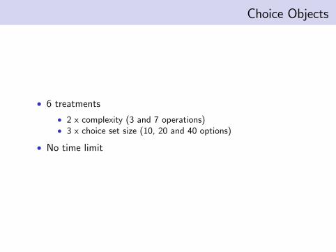
� 6 treatments� 2 x complexity (3 and 7 operations)� 3 x choice set size (10, 20 and 40 options)
� No time limit

Size 10, Complexity 3

Size 20, Complexity 7

ResultsFailure rates (%) (22 subjects, 657 choices)
Failure rateComplexity
Set size 3 710 7% 24%20 22% 56%40 29% 65%

ResultsAverage Loss ($)
Average Loss ($)Complexity
Set size 3 710 0.41 1.6920 1.10 4.0040 2.30 7.12

What Might We Want to Explain With BoundedRationality
� Random Choice
� Status Quo Bias� Failure to Choose the Best Option� Salience/Framing E¤ects� Too Much Choice� Statistical Biases� Compromise E¤ect

Salience (Chetty, Looney and Kroft, 2009)
� Experiment in supermarket� Posted prices usually exclude sales tax� Post (in addition) prices including sales tax� Reduced demand for these good by about 8%� In same supermarket, archival data shows that, for alcohol,elasticity with respect to sales tax changes order of magnitudeless that elasticity with respect to price changes

What Might We Want to Explain With BoundedRationality
� Random Choice
� Status Quo Bias� Failure to Choose the Best Option� Salience/Framing E¤ects� Too Much Choice� Statistical Biases� Compromise E¤ect

Too Much Choice (Iyengar and Lepper 2000)
� Set up a display of jams in a local supermarket� Two treatments:
� Limited choice �6 Jams� Extensive choice �24 Jams
� Record what proportion of people stopped at each display� And proportion of people bought jam conditional on stopping

Too Much Choice (Iyengar and Lepper 2000)
� Slightly more people stopped to look at the display in theextensive choice treatment:
� 60% Extensive choice treatment� 40% Limited choice treatment
� Far more people chose to buy jam, conditional on stopping, inthe Limited choice treatment
� 3% Extensive choice treatment� 31% Limited choice treatment

Too Much Choice and Simplicity Seeking (Iyengar andKamenica 2010)

Too Much Choice and Simplicity Seeking (Iyengar andKamenica 2010)

Too Much Choice and Simplicity Seeking (Iyengar andKamenica 2010)

Too Much Choice and Simplicity Seeking (Iyengar andKamenica 2010)

What Might We Want to Explain With BoundedRationality
� Random Choice
� Status Quo Bias� Failure to Choose the Best Option� Salience/Framing E¤ects� Too Much Choice� Statistical Biases� Compromise E¤ect

Gambler�s Fallacy (Croson and Sundali 2005)
� Proportion of Gambler�s Fallacy bets in casino gambling

Hot Hands Fallacy (O¤erman and Sonnemans 2000)
� Two types of coin� �Fair�: Independent� �Unfair�: Repeat last outcome with probability 70%
� Prior distribution: 50/50� Subjects observe 20 coin �ips, then report probability of unfaircoin

Gambler�s Fallacy (Croson and Sundali 2005)
� For each subject, proportion that overestimate probability ofunfair coin

What Might We Want to Explain With BoundedRationality
� Random Choice
� Status Quo Bias� Failure to Choose the Best Option� Salience/Framing E¤ects� Too Much Choice� Statistical Biases� Compromise E¤ect

Compromise E¤ect (Simonsen 1989)
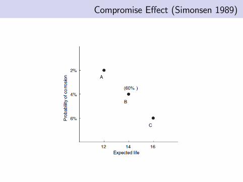
Compromise E¤ect (Simonsen 1989)
Satis�cing as Optimal Stopping
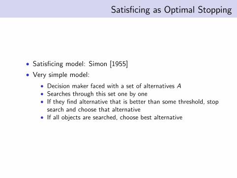
� Satis�cing model: Simon [1955]� Very simple model:
� Decision maker faced with a set of alternatives A� Searches through this set one by one� If they �nd alternative that is better than some threshold, stopsearch and choose that alternative
� If all objects are searched, choose best alternative

Satis�cing as Optimal Stopping
� Usually presented as a compelling description of a �choiceprocedure�
� Can also be derived as optimal behavior as a simple sequentialsearch model with search costs
� Primitives� A set A containing M items from a set X� A utility function u: X ! R
� A probability distribution f :decision maker�s beliefs about thevalue of each option
� A per object search cost k

The Stopping Problem
� At any point DM has two options
1 Stop searching, and choose the best alternative so far seen(search with recall)
2 Search another item and pay the cost k
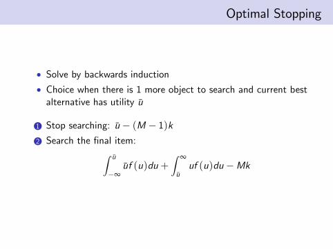
Optimal Stopping
� Solve by backwards induction� Choice when there is 1 more object to search and current bestalternative has utility u
1 Stop searching: u � (M � 1)k2 Search the �nal item:Z u
�∞uf (u)du +
Z ∞
uuf (u)du �Mk

Optimal Stopping
� Stop searching if
u � (M � 1)k � Z u
�∞uf (u)du +
Z ∞
uuf (u)du �Mk
� Implyingk �
Z ∞
u(u � u) f (u)du
� Cuto¤ strategy: search continues if u > u� solving
k =Z ∞
u�(u � u�) f (u)du (1)

Optimal Stopping
� Now consider behavior when there are 2 items remaining� u < u� Search will continue
� Search optimal if one object remaining� Can always operate continuation strategy of stopping aftersearching only one more option
� u > u� search will stop� Not optimal to search one more item only� Search will stop next period, as u > u�

Optimal Stopping
� Optimal stopping strategy is satis�cing:� Find u� that solves
k =Z ∞
u�(u � u�) f (u)du
� Continue searching until �nd an object with u > u�, then stop� Predictions about how reservation level changes withenvironment
� u� decreasing in k� increasing in variance of f (for well behaved distributions)� Una¤ected by the size of the choice set
� Comes from optimization, not reduced form satis�cing model
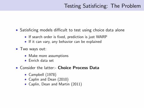
Testing Satis�cing: The Problem
� Satis�cing models di¢ cult to test using choice data alone� If search order is �xed, prediction is just WARP� If it can vary, any behavior can be explained
� Two ways out:� Make more assumptions� Enrich data set
� Consider the latter:- Choice Process Data� Campbell (1978)� Caplin and Dean (2010)� Caplin, Dean and Martin (2011)

Characterizing the Satis�cing Model
� Two main assumptions
1 Search is alternative-based� DM searches through items in choice set sequentially� Completely understands each item before moving on to thenext
2 Stopping is due to a �xed reservation rule� Subjects have a �xed reservation utility level� Stop searching if and only if �nd an item with utility abovethat level

Choice Process Data
� In order to test predictions of our model we introduce �choiceprocess�data
� Records how choice changes with contemplation time� C (A): Standard choice data - choice from set A� CA(t): Choice process data - choice made from set A aftercontemplation time t

Notation
� X : Finite grand choice set� X : Non-empty subsets of X� Z 2 fZtg∞
t : Sequences of elements of X� Z set of sequences Z
� ZA � Z : set of sequences s.t. Zt � A 2 X

A De�nition of Choice Process
De�nitionA Choice Process Data Set (X ,C ) comprises of:
� �nite set X� choice function C : X ! Z
such that C (A) 2 ZA 8 A 2 X
� CA(t): choice made from set A after contemplation time t

Alternative-Based Search (ABS)
� DM has a �xed utility function
� Searches sequentially through the available options,� Always chooses the best alternative of those searched� May not search the entire choice set� �Standard�model of information search within economics
� Stigler [1960]� McCall [1970]
� (We will consider other forms of information acquisition nextlecture)
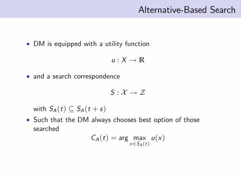
Alternative-Based Search
� DM is equipped with a utility function
u : X ! R
� and a search correspondence
S : X ! Z
with SA(t) � SA(t + s)� Such that the DM always chooses best option of thosesearched
CA(t) = arg maxx2SA(t)
u(x)

Revealed Preference and ABS
� Finally choosing x over y does not imply (strict) revealedpreference
� DM may not know that y was available
� Replacing y with x does imply (strict) revealed preference� DM must know that y is available, as previously chose it� Now chooses x , so must prefer x over y
� Choosing x and y at the same time reveals indi¤erence� Use �ABS to indicate ABS strict revealed preference� Use �ABS to indicate revealed indi¤erence

Characterizing ABS
� Choice process data will have an ABS representation if andonly if �ABS and �ABS can be represented by a utilityfunction u
x � ABSy ) u(x) > u(y)
x � ABSy ) u(x) = u(y)
� Necessary and su¢ cient conditions for utility representationwell known:
� Let �ABS=�ABS [ �ABS� Then if
x1 �ABS x2, ..., xn�1 �ABS xn �ABS x1
� then there is no k such that xk �ABS xk+1� We call this condition Only Weak Cycles

Theorem 1
TheoremChoice process data admits an ABS representation if and only if�ABS and �ABS satisfy Only Weak Cycles

Satis�cing
� Choice process data admits an satis�cing representation ifwe can �nd
� An ABS representation (u,S)� A reservation level ρ
� Such that search stops if and only if an above reservationobject is found
� If the highest utility object in SA(t) is above ρ, search stops� If it is below ρ, then search continues
� Implies complete search of sets comprising only ofbelow-reservation objects

Revealed Preference and Satis�cing
� Final choice can now contain revealed preference information� If �nal choice is below-reservation utility
� How do we know if an object is below reservation?� If they are non-terminal: Search continues after that objecthas been chosen

Directly and Indirectly Non-Terminal Sets
� Directly Non-Terminal: x 2 XN if� x 2 CA(t)� CA(t) 6= CA(t + s)
� Indirectly Non Terminal: x 2 X I if� for some y 2 XN� x , y 2 A and y 2 limt!∞ CA(t)
� Let X IN = X I [ XN

Add New Revealed Preference Information
� If� one of x ,y 2 A is in X IN� x is �nally chosen from some set A when y is not,
� then, x �S y� If x is is in X IN , then A must have been fully searched, and sox must be preferred to y
� If y is in X IN , then either x is below reservation level, in whichcase the set is fully searched, or x is above reservation utility
� Let �=�S [ �ABS

Theorem 2
TheoremChoice process data admits an satis�cing representation if and onlyif � and �ABS satisfy Only Weak Cycles

Experimental Design
� Experimental design has two aims� Identify choice �mistakes�� Test satis�cing model as an explanation for these mistakes
� Two design challenges� Find a set of choice objects for which �choice quality�isobvious and subjects do not always choose best option
� Find a way of eliciting �choice process data�
� We �rst test for �mistakes�in a standard choice task...� ... then add choice process data in same environment
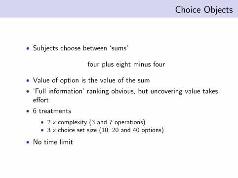
Choice Objects
� Subjects choose between �sums�
four plus eight minus four
� Value of option is the value of the sum� �Full information�ranking obvious, but uncovering value takese¤ort
� 6 treatments� 2 x complexity (3 and 7 operations)� 3 x choice set size (10, 20 and 40 options)
� No time limit

Size 10, Complexity 3
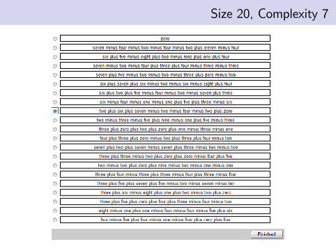
Size 20, Complexity 7

ResultsFailure rates (%) (22 subjects, 657 choices)
Failure rateComplexity
Set size 3 710 7% 24%20 22% 56%40 29% 65%

ResultsAverage Loss ($)
Average Loss ($)Complexity
Set size 3 710 0.41 1.6920 1.10 4.0040 2.30 7.12

Eliciting Choice Process Data
1 Allow subjects to select any alternative at any time
� Can change selection as often as they like
2 Choice will be recorded at a random time between 0 and 120seconds unknown to subject
� Incentivizes subjects to always keep selected current bestalternative
� Treat the sequence of selections as choice process data
3 Round can end in two ways
� After 120 seconds has elapsed� When subject presses the ��nish�button� We discard any rounds in which subjects do not press ��nish�
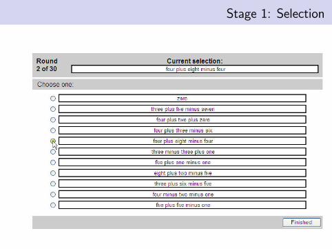
Stage 1: Selection

Stage 2: Choice Recorded
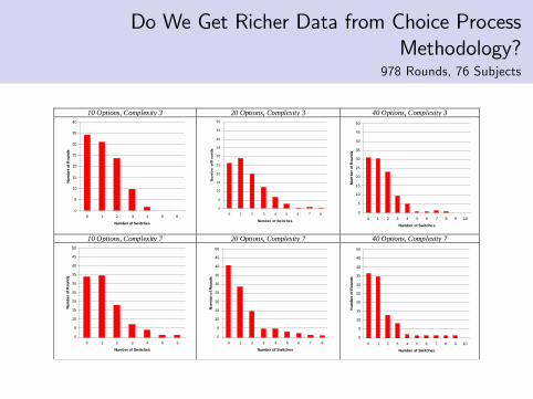
Do We Get Richer Data from Choice ProcessMethodology?
978 Rounds, 76 Subjects
10 Options, Complexity 3 20 Options, Complexity 3 40 Options, Complexity 3
0
5
10
15
20
25
30
35
40
0 1 2 3 4 5 6
Number of Switches
Num
ber o
f Rou
nds
0
5
10
15
20
25
30
35
40
45
50
0 1 2 3 4 5 6 7 8
Number of Switches
Num
ber
of R
ound
s0
5
10
15
20
25
30
35
40
45
50
0 1 2 3 4 5 6 7 8 9 10
Number of Switches
Num
ber o
f Rou
nds
10 Options, Complexity 7 20 Options, Complexity 7 40 Options, Complexity 7
0
5
10
15
20
25
30
35
40
45
50
0 1 2 3 4 5 6
Number of Switches
Num
ber o
f Rou
nds
0
5
10
15
20
25
30
35
40
45
50
0 1 2 3 4 5 6 7 8
Number of Switches
Num
ber o
f Rou
nds
0
5
10
15
20
25
30
35
40
45
50
0 1 2 3 4 5 6 7 8 9 10
Number of SwitchesN
umbe
r of R
ound
s
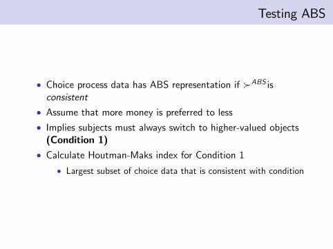
Testing ABS
� Choice process data has ABS representation if �ABS isconsistent
� Assume that more money is preferred to less� Implies subjects must always switch to higher-valued objects(Condition 1)
� Calculate Houtman-Maks index for Condition 1� Largest subset of choice data that is consistent with condition

Houtman-Maks Measure for ABS
0.1
.2.3
.4Fr
actio
n of
sub
ject
s
.6 .7 .8 .9 1HM index
Actual data0
.1.2
.3.4
Frac
tion
of s
ubje
cts
.4 .6 .8 1HM index
Random data

Traditional vs ABS Revealed Preference
Traditional ABS
0.89
0.77
0.67
0.540.49
0.23
0.2
.4.6
.81
Frac
tion
of c
hoic
es
Complexity 3 Complexity 710 20 40 10 20 40
0.970.94 0.95
0.840.82
0.86
0.2
.4.6
.81
HM
inde
xComplexity 3 Complexity 7
10 20 40 10 20 40

Satis�cing Behavior
10 20 40
3
7

Estimating Reservation Levels
� Choice process data allows observation of subjects� Stopping search� Continuing to search
� Allows us to estimate reservation levels� Assume that reservation level is calculated with some noise ateach switch
� Can estimate reservation levels for each treatment usingmaximum likelihood
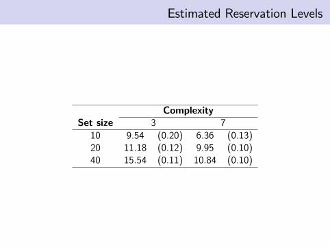
Estimated Reservation Levels
ComplexitySet size 3 710 9.54 (0.20) 6.36 (0.13)20 11.18 (0.12) 9.95 (0.10)40 15.54 (0.11) 10.84 (0.10)

Estimating Reservation Levels
� Increase with �Cost of Search�� In line with model predictions
� Increase with size of choice set� In violation of model predictions

HM Indices for Estimated Reservation Levels
ComplexitySet size 3 710 0.90 0.8120 0.87 0.7840 0.82 0.78

Does Choice Process Elicitation Change Behavior?
� In �standard choice�experiment subjects could makeintermediate selections
� Were not incentivized to do so, but did so anyway� Can use this to explore the e¤ect of choice process elicitation
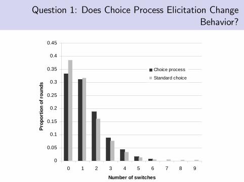
Question 1: Does Choice Process Elicitation ChangeBehavior?
0
0.05
0.1
0.15
0.2
0.25
0.3
0.35
0.4
0.45
0 1 2 3 4 5 6 7 8 9
Number of switches
Prop
ortio
n of
roun
ds
Choice process
Standard choice

Does Standard Choice Experiment Also Have SequentialSearch?
0.1
.2.3
.4Fr
actio
n of
sub
ject
s
.6 .7 .8 .9 1HM index
Choice process0
.2.4
.6Fr
actio
n of
sub
ject
s
.5 .6 .7 .8 .9 1HM index
Standard choice

Satis�cing Behavior in Standard Choice Environment
10 20 40
3
7

How Does Choice Process Elicitation Change Incentives?
� Frame as an optimal stopping problem (within ABSframework)
� Assume� Fixed cost of search� Value of objects drawn from a �xed distribution
� Can formulate optimal strategy

Di¤erences in Optimal Strategy
� Fixed reservation optimal in standard choice but decliningreservation optimal in choice process
� No good evidence for declining reservation level in either case
� Choice process environment should also always have lowerreservation levels that standard choice
� Weak evidence for this
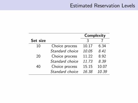
Estimated Reservation Levels
ComplexitySet size 3 710 Choice process 10.17 6.34
Standard choice 10.05 8.4120 Choice process 11.22 8.92
Standard choice 11.73 8.3940 Choice process 15.15 10.07
Standard choice 16.38 10.39

Alternative Models
� Reservation stopping time� Complete search with calculation errors

Reservation Stopping Time?
10 20 40
3
7

Complete Search with Calculation Errors
� An alternative explanation for suboptimal choice� Subjects look at all objects, but make calculation errors� Estimate logistic random error model of choices
� Scale factor allowed to vary between treatment
� Select scale factor to maximize likelihood of observed choices

Calculation Errors
� Extremely large errors needed to explain mistakes
Estimated standard deviationsComplexity
Set size 3 710 1.90 3.3420 2.48 4.7540 3.57 6.50

Calculation Errors
� Still underpredict magnitude of losses
Failure RateComplexity
10 Actual choices 11.38 46.53Simulated choices 8.35 32.47
20 Actual choices 26.03 58.72Simulated choices 20.13 37.81
40 Actual choices 37.95 80.86Simulated choices 25.26 44.39
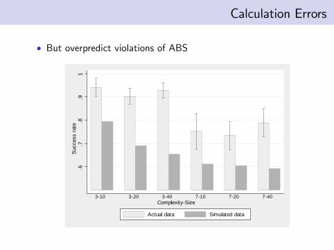
Calculation Errors
� But overpredict violations of ABS
.6.7
.8.9
1S
ucce
ss r
ate
310 320 340 710 720 740ComplexitySize
Actual data Simulated data

Estimating Reservation Levels
� Incomplete information search provides a good explanation forsuboptimal choice in this environment
� Subjects behave in line with satis�cing model� Search sequentially through choice set� Stop searching when �nding object above reservation utility
� Environmental factors change behavior, but within satis�cingframework

Related Literature
� Previous studies have used eye tracking/mouselab to examineprocess of information search
� Payne, Bettman and Johnson [1993]� Gabaix, Laibson, Moloche and Weinberg [2006]� Reutskaja, Pulst-Korenberg, Nagel, Camerer and Rangel.[2008]
� Modelled choice data with consideration sets and orderedsearch
� Rubinstein and Salant [2006]� Manzini and Mariotti [2007]� Masatlioglu and Nakajima [2008]

ResultsExperiment 1
Set Size Total3 7
10 Failure Rate (%) 6.78 23.61 16.03Average Loss ($) 0.41 1.69 1.11Average Loss (%) 3.44 13.66 9.05Observations 59 72 131
20 Failure Rate (%) 21.97 56.06 39.02Average Loss ($) 1.10 4.00 2.55Average Loss (%) 7.07 24.70 15.89Observations 132 132 264
40 Failure Rate (%) 28.79 65.38 46.95Average Loss ($) 2.30 7.12 4.69Average Loss (%) 10.49 33.25 21.79Observations 132 130 262
Total Failure Rate (%) 21.98 52.69 37.60Average Loss ($) 1.46 4.72 3.12Average Loss (%) 7.81 25.65 16.88Observations 323 334 657
ComplexityTable 1: Magnitude of Mistakes, Experiment 1

ResultsExperiment 2
Set Size Total3 7
10 Choice Process 0.42 3.69 1.90Normal Choice 0.41 1.69 1.11
20 Choice Process 1.63 4.51 2.88Normal Choice 1.10 4.00 2.55
40 Choice Process 2.26 8.30 5.00Normal Choice 2.30 7.12 4.69
Total Choice Process 1.58 5.73 3.43Normal Choice 1.46 4.72 3.12
Set Size Total3 7
10 123 101 22420 225 172 39740 195 162 357
Total 543 435 978
Number of Observations Choice ProcessComplexity
ComplexityAbsolute Loss


