Bounds for the stationary stochastic response of truss structures with uncertain-but-bounded...

Contents lists available at SciVerse ScienceDirect

Mechanical Systems and Signal Processing

Mechanical Systems and Signal Processing 37 (2013) 163–181

0888-32

http://d

n Corr

E-m

journal homepage: www.elsevier.com/locate/ymssp

Bounds for the stationary stochastic response of trussstructures with uncertain-but-bounded parameters

Giuseppe Muscolino a,n, Alba Sofi b

a Department of Civil Engineering and Inter-University Centre of Theoretical and Experimental Dynamics, University of Messina,

Villaggio S. Agata, 98166 Messina, Italyb Dipartimento di Meccanica e Materiali (MECMAT), Universit �a ‘‘Mediterranea’’ di Reggio Calabria, Via Graziella, Localit �a Feo di Vito,

89122 Reggio Calabria, Italy

a r t i c l e i n f o

Article history:

Received 13 December 2011

Received in revised form

23 May 2012

Accepted 19 June 2012Available online 18 July 2012

Keywords:

Uncertain-but-bounded parameters

Complex interval analysis

Stationary Gaussian random excitation

Frequency domain approach

Sherman–Morrison–Woodbury formula

70/$ - see front matter & 2012 Elsevier Ltd. A

x.doi.org/10.1016/j.ymssp.2012.06.016

esponding author. Tel.: þ39 90 3977159.

ail addresses: [email protected] (G. Musc

a b s t r a c t

The aim of the present paper is to determine the region of the probabilistic

characteristics of the stationary stochastic response (mean-value vector, power spectral

density function and covariance matrix) of truss structures with uncertain-but-

bounded parameters under stationary multi-correlated Gaussian random excitation

via interval analysis. The main steps of the proposed procedure are: i) to express the

stiffness, damping and mass matrices of the structural system as linear functions of the

uncertain-but-bounded parameters; ii) to split the probabilistic characteristics of the

nodal interval stationary stochastic response, evaluated in the frequency domain, as

sum of the midpoint and deviation values; iii) to evaluate in explicit approximate form

the parametric interval frequency response function matrix. The effectiveness of the

presented procedure is demonstrated by analyzing a truss structure with uncertain-

but-bounded axial stiffness and lumped masses subjected to stationary multi-corre-

lated Gaussian wind excitations.

& 2012 Elsevier Ltd. All rights reserved.

1. Introduction

The main dynamic excitations arising from natural phenomena, such as earthquake ground motion, gusty winds or seawaves, are commonly modeled as Gaussian stochastic processes for structural analysis purposes. In the framework ofStochastic Mechanics, several approaches have been proposed to cope with the challenging problem of characterizing therandom response of a structural system under stochastic excitation. In particular, it is well-known that the randomresponse is fully defined from a probabilistic point of view by the knowledge of its probability density function (PDF).Moreover, if the system has a linear behavior and it is forced by a Gaussian random process, the response is Gaussian too.In this case, the probabilistic characterization of the stochastic response can be performed either in the so-called time

domain by evaluating the mean-value vector and the correlation function matrix, or in the so-called frequency domain

through the knowledge of the mean-value vector and the power spectral density (PSD) function matrix (see e.g. [1,2]).Another class of uncertainties occurring in engineering problems is the one associated with fluctuations of structural

parameters, such as geometrical and mechanical properties or mass density. These sources of uncertainty, which affect to acertain extent the structural response, are usually described following two contrasting points of view, known asprobabilistic and non-probabilistic approaches. In the framework of the so-called probabilistic approaches, the uncertainstructural parameters are modeled as random variables with given PDF. The associated random structural response is

ll rights reserved.

olino), [email protected] (A. Sofi).

www.elsevier.com/locate/ymssp

www.elsevier.com/locate/ymssp

dx.doi.org/10.1016/j.ymssp.2012.06.016

dx.doi.org/10.1016/j.ymssp.2012.06.016

dx.doi.org/10.1016/j.ymssp.2012.06.016

http://crossmark.dyndns.org/dialog/?doi=10.1016/j.ymssp.2012.06.016&domain=pdf



mailto:[email protected]

mailto:[email protected]

dx.doi.org/10.1016/j.ymssp.2012.06.016

G. Muscolino, A. Sofi / Mechanical Systems and Signal Processing 37 (2013) 163–181164

usually predicted following three main ways: the Monte Carlo simulation method, the stochastic finite element method [3]and the spectral approach [4]. A discussion on the application of probabilistic approaches to the case of truss structures canbe found in Ref. [5,6].

Despite their success, unfortunately the probabilistic approaches give reliable results only when sufficient experimentaldata are available to define the PDF of the fluctuating properties. If available information are fragmentary or incomplete sothat only bounds on the magnitude of the uncertain structural parameters are known, non-probabilistic approaches, suchas convex models, fuzzy set theory or interval models, can be alternatively applied [7]. The interval model, which stemsfrom interval analysis (see e.g. [8–11]), may be considered as the most widely used analytical tool among non-probabilisticmethods. According to this approach, the fluctuating structural parameters are treated as interval numbers with givenlower and upper bounds. The application of the interval analysis method to practical engineering problems is not an easytask due to the complexity of the related algorithms. In the literature, in the case of slight parameter fluctuations anddeterministic loads, the so-called Interval Perturbation Method (IPM) or, equivalently, the First-Order Interval Taylor Series

Expansion have been successfully adopted to perform both static [12–16] and dynamic structural analysis [17–19]. Themain advantages of these methods are the flexibility and the simplicity of the mathematical formulation.

In the framework of Stochastic Mechanics, the IPM has been extended by the authors [20,21] to cope also with randomlyexcited structures. However, since the effectiveness of perturbation-based approaches is limited to small parameterfluctuations and the effect of neglecting the higher-order terms is unpredictable, recently the authors proposed an alternativeapproach, to characterize, in the time domain, the stochastic response due to both stationary [22] or non-stationary [23,24]random excitations. Notably, in these papers, the drawbacks associated with the so-called dependency phenomenon areovercome. This phenomenon [11,25,26] frequently occurs in the ‘‘ordinary’’ interval analysis when an expression containsmultiple instances of one or more interval variables. Indeed, the ‘‘ordinary’’ interval analysis, mainly based on the formulationderived by Moore [8], often leads to an overestimation of the interval solution width that could be catastrophic from anengineering point of view. This happens when the operands are partially dependent on each other so that not all combinationsof values in the given intervals will be valid and the exact interval will be smaller than the one produced by the formulas.

Interval-based uncertainty models have been extensively used in the context of static (see e.g. [27–29]) and dynamic(see e.g. [19,30,31]) finite element analysis of structures. A general overview of the state-of-art and recent advances ininterval finite element analysis can be found in Ref. [26,32], where the two fundamental approaches are described indetails: the interval arithmetic strategy and the global optimization approach. The application of interval arithmetic basedfinite element methods is hindered by the dependency phenomenon which introduces conservatism not only in thesolution phase, but also in the assembly of the system matrices. In the literature, several attempts have been made to limitconservatism, such as the element-by-element technique developed by Muhanna and Mullen [25] or the improvement ofinterval finite element analysis proposed by Degrauwe et al. [33] based on affine arithmetic.

As far as the case of random input is concerned, in all the studies carried out by the authors the uncertain-but-boundedstochastic response is characterized in the time domain by solving a set of linear algebraic equations or a set of first-orderdifferential equations, depending on whether the excitation is stationary or non-stationary, respectively. Both these sets ofequations are derived by applying the Kronecker algebra [34]. The main computational drawback of the time domainformulation is associated with the evaluation of the input-output cross-correlation appearing in the forcing term, whichcan be determined in closed-form only for white or filtered white stochastic input processes.

The aim of the present paper is to determine the region of the random response of truss structures with uncertain-but-bounded parameters under stationary multi-correlated Gaussian stochastic excitation by applying the complex interval

analysis [9] within the context of the frequency domain approach. Unfortunately, the ‘‘ordinary’’ complex interval analysissuffers from the dependency phenomenon too. In the framework of the so-called affine arithmetic [35,36], Manson [37]proposed an approach which allows to take into account the dependency between the real and imaginary components ofthe complex interval variables. In the present paper, the catastrophic effects of the dependency phenomenon are limited byadopting an improvement of the ordinary complex interval analysis, based on the philosophy of the affine arithmetic. Theproposed procedure basically requires the following steps: i) the decomposition of the stiffness, damping and mass matricesof the structural system as sum of the nominal value plus a deviation given as a linear function of the uncertain-but-bounded parameters; ii) the evaluation in explicit approximate form of the parametric interval transfer function matrix, byapplying the so-called rational series expansion recently proposed by Muscolino et al. [38], and of the inverse of the intervalstiffness matrix by using the extended interval-valued Sherman–Morrison–Woodbury formula derived by Impollonia andMuscolino [39]; iii) the determination of the upper and lower bounds of the probabilistic characteristics of the nodalstationary stochastic interval response (mean-value vector, power spectral density functions and covariance matrix).

Numerical results concerning a truss structure with uncertain-but-bounded axial stiffness and lumped masses understationary multi-correlated Gaussian wind excitations are presented to show the effectiveness of the proposed method.

2. Problem formulation

2.1. Preliminary definitions: real and complex interval variables

In this paper, the attention is focused on truss structures with uncertain-but-bounded structural properties understationary Gaussian random excitation. Following a standard formulation, the stiffness, damping and mass matrices of a

G. Muscolino, A. Sofi / Mechanical Systems and Signal Processing 37 (2013) 163–181 165

n-degree-of-freedom (n-DOF) truss structure can be written as functions of r uncertain-but-bounded structural parametersai, collected in the r-order vector a. Such parameters are assumed independent. Furthermore, according to the intervalanalysis [8,11], denoting by IR the set of all closed real interval numbers, the bounded set-interval vector of real numbersaI9½a,a� 2 IRr , such that arara, can be introduced. The symbols a and a denote the lower and upper bound vectors.Since the real numbers ai are bounded by intervals, the relevant mathematical derivations should be performed by meansof the ‘‘ordinary’’ interval analysis [8–11]. However, the ‘‘ordinary’’ interval analysis suffers from the so-called dependency

phenomenon [11,25,26] which often leads to an overestimation of the interval width that could be catastrophic from anengineering point of view. This occurs when an expression contains multiple instances of one or more interval variables.Indeed, the ordinary interval arithmetic operations assume that the operand interval numbers are independent. When theoperands are partially dependent on each other, not all combinations of values in the given intervals will be valid and theexact result interval will generally be smaller than the one produced by the formulas.

To limit the catastrophic effects of the dependency phenomenon, the so-called generalized interval analysis [40] and theaffine arithmetic [35,36] have been introduced in the literature. In these formulations, each intermediate result isrepresented by a linear function with a small remainder interval [41]. According to the philosophy of the affine arithmetic, anew definition of the extra symmetric unitary interval (NEUI) variable e

Ii9½�1,þ1� ði¼ 1,2,UUU,rÞ is herein proposed as a

proper extension of the EUI variable recently introduced by the authors [24]. The NEUI turns out to be more suitable for theprobabilistic characterization of the interval stationary stochastic response herein addressed and it is defined in such away that the following properties hold:

eIi�e

Ii ¼ 0; e

Ii � e

Ii ¼ ðe

IiÞ

2¼ ½1,1�;

eIi � e

Ij ¼ ½�1,þ1�, iaj; e

Ii=e

Ii ¼ ½1,1�;

xieIi 7yie

Ii ¼ ðxi7yiÞe

Ii ;

xieIi � yie

Ii ¼ xiyiðe

IiÞ

2¼ xiyi½1,1�; ðxie

IiÞ

k¼

xki ½1,1� for k even,

xki e

Ii for k odd:

8<:

ð1a� gÞ

In these equations, [1,1]¼1 is the so-called unitary thin interval. It is useful to remember that a thin interval occurswhen x ¼ x and it is defined as xI9½x,x�, so that x 2 R.

Then, introducing the midpoint value (or mean), a0,i, and the deviation amplitude (or radius), Dai, of the i-th realinterval variable aI

i:

a0,i ¼1

2ða iþaiÞ; Dai ¼

1

2ðai�a iÞ, ð2a;bÞ

the following affine form definition can be adopted:

aIi ¼ a0,iþDaie

Ii , ði¼ 1,2,:::,rÞ: ð3Þ

Furthermore, denoting by a0 and Da the vectors collecting the midpoint values (or mean values) and the radii (ordeviation amplitudes), a0,i and Dai, respectively, of the interval parameters aI

i , (i¼1,2,...,r), one can write:

a0 ¼1

2ðaþaÞ; Da¼

1

2ða�aÞ: ð4a;bÞ

In the case of complex interval variables, within the framework of the affine arithmetic, Manson [37] proposed anapproach which allows to take into account the dependency between the real and imaginary components of the complexvariables. Conversely, the ‘‘ordinary’’ complex interval analysis assumes that the real and imaginary components areindependent. According to the philosophy of the affine arithmetic, a complex interval variable zI

i ¼ xIiþ iyI

i is herein defined as

zIi ¼ z0,iþDzie

Ii ¼ ðx0,iþ iy0,iÞþðDxiþ iDyiÞe

Ii ð5Þ

where i¼ffiffiffiffiffiffiffi�1p

denotes the imaginary unit; x0,i and y0,i are the midpoint values (or means) and D xi and D yi are the deviationamplitudes (or radii) of the real and imaginary part of the complex interval variable, respectively. They are given,respectively, as

x0,i ¼12 ðxiþxiÞ; y0,i ¼

12 ðyiþyiÞ;

Dxi ¼12 ðxi�xiÞ; Dyi ¼

12 ðyi�y

iÞ:

ð6a� dÞ

2.2. Equations of motion

The equations of motion of a quiescent n-DOF classically damped linear truss structure with uncertain-but-boundedstructural properties subjected to a stationary multi-correlated Gaussian stochastic process f(t) can be cast in the form:

MðaÞ €uða,tÞþCðaÞ _uða,tÞþKðaÞuða,tÞ ¼ fðtÞ, a 2 aI ¼ ½a,a� ð7Þ


where M(a), C(a) and K(a) are the n�n mass, damping and stiffness matrices of the structure which depend on theuncertain parameters collected in the vector a of order r; u(a,t) is the stationary Gaussian vector process of nodaldisplacements and a dot over a variable denotes differentiation with respect to time t. The Rayleigh model is hereinadopted for the interval damping matrix, i.e.:

CðaÞ ¼ c0MðaÞþc1KðaÞ, a 2 aI ¼ ½a,a� ð8Þ

where c0 and c1 are the Rayleigh damping constants having units s�1 and s, respectively.In structural engineering, it can be reasonably assumed that the interval uncertainties posses symmetric deviation

amplitude ai ¼� a i � ai, so that:

a0,i ¼aiþa i

2¼ 0; Dai ¼

ai�a i

2� ai40: ð9a;bÞ

Therefore, the generic symmetric interval variable can be written as

aIi ¼Daie

Ii : ð10Þ

Following the interval formalism above introduced, the n�n order structural matrices can be expressed as linearfunctions of the uncertain properties, i.e.:

MðaÞ ¼M0þXrM

j ¼ 1

MjDajeIj ,

KðaÞ ¼K0þXrK

j ¼ 1

KjDajeIj , a 2 aI ¼ a,a

� �

CðaÞ ¼ C0þc0

XrM

j ¼ 1

MjDajeIjþc1

XrK

j ¼ 1

KjDajeIj

ð11a� cÞ

where rMþrK¼r and

M0 ¼Mða0Þ; Mj ¼@

@ajMðaÞ

��a ¼ a0

, K0 ¼Kða0Þ; Kj ¼@

@ajKðaÞ

��a ¼ a0

: ð12a� dÞ

In the previous equations, M0, K0 and C0¼c0 M0þc1 K0 denote the mass, stiffness and damping matrices of the nominalstructural system, which are positive definite symmetric matrices of order n�n; furthermore, Mj and Kj are semi-positivedefinite symmetric matrices of order n�n and Daj is the positive dimensionless fluctuation of the j-th uncertainparameter.

2.3. Frequency domain response

Performing the Fourier transform of both sides of Eq. (7) and taking into account Eqs. (11a-c), the following set ofalgebraic frequency dependent equations governing the response in the frequency domain is obtained:

�o2M0þ ioC0þK0�o2XrM

j ¼ 1

MjDajeIjþ ioc0

XrM

j ¼ 1

MjDajeIjþ ioc1

XrK

j ¼ 1

KjDajeIjþXrK

j ¼ 1

KjDajeIj

35Uða,oÞ ¼ FðoÞ

24 ð13Þ

where U(a,o) and F(o) are the vectors collecting the Fourier transforms of u(a,t) and f(t), respectively. The intervalfrequency response vector U(a,o), solution of Eq. (13), can be expressed as follows:

Uða,oÞ ¼Hða,oÞFðoÞ, a 2 aI ¼ ½a,a� ð14Þ

where H(a,o) is the frequency response function (FRF) matrix (referred to also as transfer function matrix) given as

Hða,oÞ ¼ ½H�10 ðoÞþRða,oÞ��1 ¼ ½InþH0ðoÞRða,oÞ��1H0ðoÞ, a 2 aI ¼ ½a,a�: ð15Þ

In the previous equation, In denotes the identity matrix of order n and H0(o) is the FRF matrix of the nominal structuralsystem, given by

H0ðoÞ ¼ ½�o2M0þ ioC0þK0��1 ð16Þ

and

Rða,oÞ ¼ ðioc0�o2ÞXrM

j ¼ 1

MjDajeIjþð1þ ioc1Þ

XrK

j ¼ 1

KjDajeIj , a 2 aI ¼ ½a,a� ð17Þ

is an interval complex matrix of order n�n accounting for the fluctuations of the structural parameters.Notice that for classically damped structural systems the nominal FRF matrix can be evaluated as:

H0ðoÞ ¼U0H0,mðoÞUT0 ð18Þ


where U0 is the modal matrix of order n�m (mrn) collecting the first m eigenvectors normalized with respect to themass matrix M0. This matrix is obtained as solution of the following eigenproblem:

K0U0 ¼M0U0X20; UT

0M0U0 ¼ Im ð19a;bÞ

where X20 ¼UT

0K0U0 is the spectral matrix of the nominal structural system, say a diagonal matrix listing the squares ofthe natural circular frequencies of the truss structure for the midpoint values of the uncertain parameters, i.e. a¼a0; theapex T means transpose matrix. It is worth noting that in Eq. (18) H0,m(o) is the modal transfer function matrix of thenominal structure that for classically damped structural systems can be evaluated in closed-form as

H0,mðoÞ ¼ �o2Imþ ioN0þX20

h i�1ð20Þ

where N0 ¼UT0CU0 is the generalized damping matrix, which for the Rayleigh model of damping is a diagonal one.

2.4. Stochastic response

In the framework of Stochastic Mechanics, several approaches have been proposed to cope with the challengingproblem of determining the random response of a structural system. It is well-known that the random response is fullydefined, from a probabilistic point of view, if the probability density function (PDF) of the response is known. If the systemhas a linear behavior and it is forced by a Gaussian random process, the response is Gaussian too. In this case, thestochastic response process can be characterized in the so-called time domain by evaluating the mean-value vector andthe correlation function matrix, or, alternatively, in the so-called frequency domain through the knowledge of the mean-value vector and the PSD function matrix (see e.g. [1,2]). In this paper, following the frequency domain approach, thestationary stochastic Gaussian interval response process of the truss structure with uncertain-but-bounded parameters iscompletely characterized from a probabilistic point of view by defining the interval mean-value vector, lu(a), and theinterval PSD function matrix, Suu(a,o), a 2 aI ¼ ½a,a�.

In order to evaluate the statistics of the interval structural response, it useful to preliminarily observe that, if the inputprocess f(t) is split as sum of two terms, i.e.:

fðtÞ ¼ lfþ~Xf ðtÞ ð21Þ

where lf ¼ E fðtÞ� �

is a deterministic vector denoting the mean-value of the excitation, whereas ~Xf ðtÞ is a zero-meanstationary multi-correlated Gaussian random process, the stochastic response process can be written as:

uða,tÞ ¼ luðaÞþ ~Uuða,tÞ, a 2 aI ¼ ½a,a�: ð22Þ

In the previous equation, ~Uuða,tÞ is the zero-mean stationary Gaussian stochastic interval response vector processdue to the random excitation ~Xf ðtÞ. Since the autocorrelation function of a stochastic process remains unchangedwhen a deterministic function is added, the vector ~Uuða,tÞ possesses interval correlation function matrix R ~Uu

~Uuða,tÞ ¼

E ~Uuða,t1Þ~U

T

uða,t2Þ

D E� Ruu(a,t) and interval PSD function matrix S ~Uu

~Uuða,oÞ � Suu(a,o).

The mean-value of the response process governed by Eq. (7), where the input is the mean-value lf ¼ E fðtÞ� �

of theexcitation f(t), can be determined once the inverse of the interval stiffness matrix is evaluated, that is:

luðaÞ ¼K�1ðaÞlf , a 2 aI ¼ ½a,a�: ð23Þ

On the other hand, to obtain the second-order statistics of the interval stochastic response in the frequency domain, theresponse PSD function matrix has to be evaluated. It is well-known that this matrix is related to the PSD function matrix ofthe zero-mean stationary Gaussian stochastic input, S ~Xf

~XfðoÞ, by means of the following relationship [2]:

Suuða,oÞ ¼Hnða,oÞS ~Xf

~XfðoÞHT

ða,oÞ, a 2 aI ¼ ½a,a� ð24Þ

where the asterisk means complex conjugate and H(a,o) is the FRF matrix given in Eq. (15).Hence, in order to characterize the interval stochastic response process, the interval transfer function matrix H(a,o)

(see Eqs. (15) and (24)) and the inverse of the interval stiffness matrix K�1 (a) (see Eq. (23)) have to be computed. In thenext section, these inverse matrices will be evaluated in explicit approximate form by applying the so-called rational series

expansion (RSE), recently proposed by the authors [38], and the extended interval-valued Sherman–Morrison–Woodbury

(SMW) formula [39], respectively.

3. Approximate interval transfer function matrix

In this section, an approximate explicit expression of the transfer function matrix H(a,o) for truss structural systemswith uncertain parameters is derived. This explicit expression is very useful for numerical purposes, since it allows toavoid the onerous inversion of the full frequency-dependent interval matrix between square brackets in Eq. (15).

In the case of truss structures, composed of s bar elements and having n-DOF, the n�n stiffness matrix can bedefined as:

K¼ GT EG ð25Þ


where GT is the n� s equilibrium matrix (whose transpose is the so-called compatibility matrix) and E is the s� s diagonalinternal stiffness matrix. Let us now indicate with rj ¼ EjAj=Lj the axial stiffness of the j-th bar element and assume thatrKrs elements possess uncertain-but-bounded axial stiffness. Denoting with Dajo1 the symmetric fluctuation of theuncertain axial stiffness around the nominal value r0,j ¼ E0,jA0,j=L0,j, one gets

rIj ¼ r0,jð1þDaje

IjÞ ð26Þ

where j¼1, 2,y, rKrs and eIj is the NEUI variable defined in Section 2.1. Then, the internal stiffness matrix E(aK) can be

written as

EðaK Þ ¼ E0þXrK

j ¼ 1

DajeIjlK ,jl

TK ,j, aK 2 aI ¼ ½a,a� ð27Þ

where E0 is the nominal internal stiffness matrix and aK is the sub-vector of a collecting the fluctuations Daj (j¼1,2,yrKrs); lK,j is a vector of order s with only the j-th element equal to

ffiffiffiffiffiffiffiffir0,j

pand the other ones equal to zero. Notice that

the dyadic product lK ,jlTK ,j gives a change of rank one to the nominal internal stiffness matrix. Then, according to Eq. (25),

also the stiffness matrix K(a) possesses rK uncertain-but-bounded parameters, and can be rewritten as

KðaK Þ ¼K0þXrK

j ¼ 1

KjDajeIj ¼K0þ

XrK

j ¼ 1

DajeIjwK ,jw

TK ,j, aK 2 aI ¼ ½a,a� ð28Þ

where K0 is the nominal stiffness matrix and wTK ,j ¼ lT

K ,jG.Similarly, the lumped mass matrix can be written as

MðaMÞ ¼M0þXrM

j ¼ 1

MjDajeIj ¼M0þ

XrM

j ¼ 1

DajeIjwM,jw

TM,j, aM 2 aI ¼ ½a,a� ð29Þ

where M0 is the diagonal nominal mass matrix whose j-th element is m0,j; aM is the sub-vector of a collecting thefluctuations Daj (j¼1, 2,yrMrn); wM,i is a vector of order n with only the j-th element equal to

ffiffiffiffiffiffiffiffiffim0,jp

and the other onesequal to zero. Notice that the dyadic product wM,jw

TM,j gives a change of rank one to the nominal mass matrix.

Finally, in the context of the Rayleigh model herein adopted, the damping matrix can be decomposed as

CðaÞ ¼ C0þc0

XrM

j ¼ 1

DajeIjwM,jw

TM,jþc1

XrK

j ¼ 1

DajeIjwK ,jw

TK ,j, a 2 aI ¼ ½a,a�: ð30Þ

Substituting Eqs. (28)–(30) into Eq. (13), the FRF matrix of the truss structure can be expressed according to Eq. (15),where the interval matrix R(a,o) takes the following form:

Rða,oÞ ¼ ðioc0�o2ÞXrM

j ¼ 1

DajeIjwM,jw

TM,jþð1þ ioc1Þ

XrK

j ¼ 1

DajeIjwK ,jw

TK ,j ¼

Xr ¼ rM þ rK

j ¼ 1

pjðoÞDajeIjwjw

Tj ð31Þ

where

pjðoÞ ¼ ðioc0�o2Þ, wj ¼wM,j for j¼ 1,2,. . .,rM;

pjðoÞ ¼ ð1þ ioc1Þ, wj ¼wK ,j for j¼ rMþ1,rMþ2,. . .,rMþrK :ð32a;bÞ

To avoid the inversion of the parametric frequency-dependent matrix in Eq. (15), for every o, the Neumann seriesexpansion could be adopted which leads to the following expression:

Hða,oÞ ¼ ½ImþH0ðoÞRða,oÞ��1H0ðoÞ ¼H0ðoÞþX1k ¼ 1

ð�1Þk½H0ðoÞRða,oÞ�kH0ðoÞ,

a 2 aI ¼ ½a,a�: ð33Þ

The convergence of this series expansion is guaranteed if and only if the least square norm of the matrix in squarebrackets is less than one. This condition is always satisfied for structural systems with uncertain parameters Daio1, 8i.

In this paper, an alternative approach is proposed which yields an approximate explicit expression of the FRF matrix.Specifically, once the interval matrix R(a,o) has been decomposed as sum of rank-one matrices (see Eq. (31)), the RSE [38]can be applied, obtaining:

Hða,oÞ ¼ H�10 ðoÞþ

Xr

i ¼ 1

piðoÞDaieIiwiw

Ti

" #�1

�H0ðoÞ�Xr

i ¼ 1

piðoÞDaieIi

1þpiðoÞDaieIibiðoÞ

BiðoÞ ð34Þ

where:

biðoÞ ¼wTi H0ðoÞwi;

BiðoÞ ¼H0ðoÞwiwTi H0ðoÞ

ð35a;bÞ


are complex quantities. Notice that Eq. (34) holds if and only if the following condition is satisfied:

JpiðoÞDaibiJo1 ð36Þ

where the symbol :�: denotes the modulus of the complex quantity �.Eq. (37) gives an approximate closed-form expression of the transfer function matrix of truss structures with uncertain-

but-bounded parameters. It has to be emphasized that this expression has been obtained by applying the RSE [38] whosefirst two terms coincide with a generalization to complex interval algebra of the so-called approximate extended interval-

valued Sherman–Morrison–Woodbury (SMW) formula [39]. This generalization involves the NEUI variable defined in Section2.1. Obviously, the accuracy of Eq. (34), which gives the explicit inverse of a matrix with r fluctuating parameters, dependson the magnitude of the fluctuations Daio1 and can be improved by retaining higher-order terms [38].

Alternatively, the approximate interval transfer function matrix in Eq. (34) H(a,o) can be rewritten in affine form asfollows:

Hða,oÞ ¼H0ðoÞþXr

i ¼ 1

a0,iðoÞþDaiðoÞeIi

h iBiðoÞ, a 2 aI ¼ ½a,a� ð37Þ

where a0, i(o) and D ai(o) are complex functions, given respectively, by

a0,iðoÞ ¼ 12 �

piðoÞDai

1þpiðoÞDaibiðoÞþ

piðoÞDai

1�piðoÞDaibiðoÞ

� ¼

piðoÞDai

�2biðoÞ

1� piðoÞDaibiðoÞ �2

;

DaiðoÞ ¼1

2

piðoÞDai

1�piðoÞDaibiðoÞþ

piðoÞDai

1þpiðoÞDaibiðoÞ

� ¼

piðoÞDai

1� piðoÞDaibiðoÞ �2

:

ð38a;bÞ

Based on Eq. (37), the interval FRF matrix can be expressed as:

Hða,oÞ ¼HmidðoÞþHdevða,oÞ, a 2 aI ¼ ½a,a� ð39Þ

where:

HmidðoÞ ¼midfHða,oÞg ¼H0ðoÞþXr

i ¼ 1

a0,iðoÞBiðoÞ;

Hdevða,oÞ ¼ devfHða,oÞg ¼Xr

i ¼ 1

DaiðoÞBiðoÞeIi

ð40a;bÞ

are two complex function matrices listing the midpoint and the deviation of the elements of H(a,o), respectively.It is worth mentioning that, for small fluctuations of the uncertain properties, the proposed approach can be

conveniently applied in the modal subspace replacing the interval modal matrix by the nominal one U0. Although afurther approximation is thus introduced, the use of modal analysis may be preferable when dealing with large-scalestructures having a high number of DOFs.

4. Bounds of the Gaussian stationary stochastic interval response

The aim of this section is to determine in the frequency domain the range of the stochastic response of linear trussstructures with uncertain-but-bounded parameters under stationary Gaussian random excitation via interval analysis. Inthe framework of Stochastic Mechanics, this task usually reduces to the evaluation of the mean-value vector and PSDfunction matrix. The region of these quantities for structures with uncertain-but-bounded parameters can be determinedby defining the bounds of the interval mean-value vector, luðaÞ 2 IR

n, and of the interval PSD function matrix,SuuðaÞ 2 IRn2

. Moreover, the knowledge of the interval PSD function matrix allows to compute the upper bound and thelower bound of the covariance matrix RuuðaÞ 2 IRn2

of the interval displacement vector.

4.1. Bounds of the interval mean-value vector

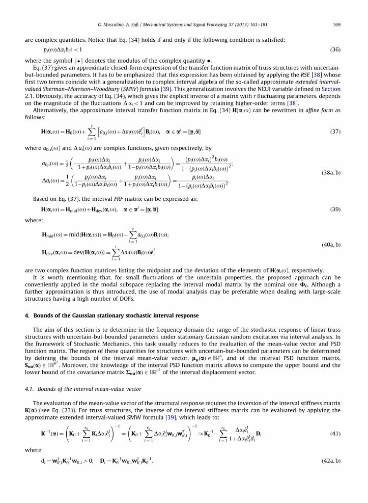
The evaluation of the mean-value vector of the structural response requires the inversion of the interval stiffness matrixK(a) (see Eq. (23)). For truss structures, the inverse of the interval stiffness matrix can be evaluated by applying theapproximate extended interval-valued SMW formula [39], which leads to:

K�1ðaÞ ¼ K0þ

XrK

i ¼ 1

KiDaieIi

!�1

¼ K0þXrK

i ¼ 1

DaieIiwK ,iw

TK ,i

!�1

�K�10 �

XrK

i ¼ 1

DaieIi

1þDaieIidi

Di ð41Þ

where

di ¼wTK ,iK

�10 wK ,i40; Di ¼K�1

0 wK ,iwTK ,iK

�10 : ð42a;bÞ


It has also been shown [39] that Eq. (41) holds if and only if the following condition is satisfied:

Daidio1, 8i: ð43Þ

Obviously, the accuracy of Eq. (41), which gives the explicit inverse of a matrix with rK fluctuating parameters, dependson the magnitude of the fluctuations Daio1.

Alternatively, by adopting the interval formalism (3), Eq. (41) can be rewritten in affine form as

K�1ðaÞ ¼ K0þ

XrK

i ¼ 1

DaieIiwK ,iw

TK ,i

!�1

�K�10 þ

XrK

i ¼ 1

ð ~a0,iþD ~aieIiÞDi ð44Þ

where ~a0, i and D ~ai are given by [39]

~a0,i ¼1

2�

Dai

1þDaidiþ

Dai

1�Daidi

� ¼

Daið Þ2di

1� Daidið Þ240;

D ~a0,i ¼1

2

Dai

1�Daidiþ

Dai

1þDaidi

� ¼

Dai

1� Daidið Þ240:

ð45a;bÞ

Notice that, for one uncertain parameter, Eq. (41) leads to the classical Sherman–Morrison formula [42,43] for the caseof rank-one modifications. Furthermore, Eq. (41) may be viewed as an extension of the procedure proposed by Rohn [44]for deriving closed-form expressions of the bounds of the inverse interval matrix in the special case of a matrix with rank-one deviation.

Substituting the approximate inverse (44) of the interval stiffness matrix K(a) into Eq. (23), the interval mean-value ofthe structural response can be expressed as follows:

luðaÞ ¼ K�10 þ

XrK

i ¼ 1

~a0,iþD ~aieIi

� Di

" #lf , a 2 aI ¼ ½a,a�: ð46Þ

Since the elements of the matrix between square brackets in Eq. (46) are monotonic functions of the generic fluctuationDai, the lower and upper bounds of this matrix can be evaluated considering the upper and lower bounds of the NEUI,e

Ii ¼ �1,1½ �, respectively. Based on this observation, Eq. (46) can be alternatively rewritten as sum of the midpoint,

mid{lu(a)}, and deviation, dev{lu(a)}, of the interval mean-value vector, i.e.:

luðaÞ ¼ K�10 þ

XrK

i ¼ 1

~a0,iþD ~aieIi

� Di

" #lf ¼midfluðaÞgþdevfluðaÞg, a 2 aI ¼ ½a,a� ð47Þ

where

midfluðaÞg ¼ K�10 þ

XrK

i ¼ 1

~a0,iDi

" #lf ;

devfluðaÞg ¼XrK

i ¼ 1

D ~aieIiDi

" #lf , a 2 aI ¼ ½a,a�:

ð48a;bÞ

Furthermore, since the deviation vector, dev{lu(a)}, defined in Eq. (48b), is a symmetric interval vector, the lowerbound, l

u, and the upper bound, lu, of the interval response mean-value vector, defined in Eq. (47), can be evaluated as

lu¼midfluðaÞg�Dlu;

lu ¼midfluðaÞgþDlu

ð49a;bÞ

where

Dlu ¼XrK

i ¼ 1

D ~ai Dilf

�� : ð50a;bÞ

with the symbol 9�9 denoting absolute value component wise.

4.2. Bounds of the interval PSD function matrix function

The evaluation of the interval PSD function matrix of the structural response, defined in Eq. (24), relies on theknowledge of the interval transfer function matrix (15) derived in explicit approximate form in Section 3. Then,substituting the interval transfer function matrix H(a,o) written in the form (39) into Eq. (24), the interval PSD functionmatrix of the structural response can be expressed as

Suuða,oÞ ¼midfSuuða,oÞgþdevfSuuða,oÞg, a 2 aI ¼ ½a,a� ð51Þ


where mid{Suu(a,o)} and dev{Suu(a,o)} are the midpoint and the deviation PSD function matrices given, respectively, by

mid Suuða,oÞ� �

¼Hn

midðoÞS ~Xf~XfðoÞHT

midðoÞ;

dev Suuða,oÞ� �

¼Hn

midðoÞS ~Xf~XfðoÞHT

devða,oÞþHn

devða,oÞS ~Xf~XfðoÞHT

midðoÞ

þHn


devða,oÞ a 2 aI ¼ ½a,a�:

ð52a;bÞ

In order to simplify interval computations, higher-order terms appearing in the deviation of the interval PSD functionmatrix (see Eq. (52b)), are neglected, namely terms associated with powers of the generic fluctuation Dai greater than oneare disregarded. According to this approximation, Eq. (52b) can be rewritten as

devfSuuðoÞg �Hn

0ðoÞS ~Xf~XfðoÞHT

devða,oÞþHn


0ðoÞ, a 2 aI ¼ ½a,a� ð53Þ

where the hat stands for approximate expression and H0(o) is the FRF matrix of the nominal structural system introduced in Eq.(16). Substituting the deviation matrix Hdev(a,o) defined in Eq. (40b) into Eq. (53), and applying the main properties of the NEUIvariable (see Eq. (1)), after very simple algebra, the approximate deviation matrix function, dev Suuða,oÞ

n o, can be written as

dev Suuða,oÞn o

¼ �DSuuðoÞ,þDSuuðoÞh i

ð54Þ

where

DSuuðoÞ ¼Xr

i ¼ 1

Hn

0ðoÞS ~Xf~XfðoÞDaiðoÞBT

i ðoÞþDan

i ðoÞBn

i ðoÞS ~Xf~XfðoÞHT

0ðoÞ�� , ð55Þ

is a real matrix which denotes the symmetric deviation amplitude of the function matrix dev Suuða,oÞn o

. Finally, the lowerbound, Su‘u‘

ðoÞ, and the upper bound, Su‘u‘ ðoÞ, of the interval PSD function of the ‘-th nodal displacement can be evaluated,respectively, as

Su‘u‘ðoÞ ¼mid Su‘u‘ ðoÞ

� ��DSu‘u‘ ðoÞ;

Su‘u‘ ðoÞ ¼mid Su‘u‘ ðoÞ� �

þDSu‘u‘ ðoÞ,ð56a;bÞ

where mid Su‘ u‘ ðoÞ� �

is the ‘-th element of the principal diagonal of the midpoint matrix mid{Suu(a,o)}, defined in Eq. (52a) andDSu‘u‘ ðoÞ denotes the (‘,‘) element of the deviation matrix DSuuðoÞ in Eq. (55).

4.3. Bounds of the interval covariance matrix

Once, the interval PSD function matrix, Suu(a,o), is known (see Eq. (51)), the interval covariance matrix of the structuralresponse can be evaluated as

RuuðaÞ ¼Z 1�1

Suuða,oÞdo¼mid RuuðaÞ� �

þdev RuuðaÞ� �

, a 2 aI ¼ ½a,a� ð57Þ

where mid{Ruu(a)} and dev{Ruu(a)} are the midpoint and deviation covariance matrices, given respectively by

mid RuuðaÞ� �

¼R1�1

mid Suuða,oÞ� �

do;dev RuuðaÞ

� �¼R1�1


do, a 2 aI ¼ ½a,a�:ð58a;bÞ

Finally, the bounds of the interval covariance matrix can be evaluated respectively as

Ruu ¼mid RuuðaÞ� �

�DRuu;

Ruu ¼mid RuuðaÞ� �

þDRuu

ð59a;bÞ

where DRuu is the approximate deviation amplitude matrix of the interval covariance matrix which takes the followingform:

DRuu ¼Xr

i ¼ 1

Z 1�1

Hn

0ðoÞS ~Xf~XfðoÞDaiðoÞBT

i ðoÞþDan

i ðoÞBn


0ðoÞ�� do: ð60Þ

The lower bound, Su‘u‘, and the upper bound, Su‘u‘ , of the interval covariance function of the ‘-th nodal displacement

can be evaluated, respectively, as

Su‘u‘¼mid Su‘u‘

� ��DSu‘u‘ ;

Su‘u‘ ¼mid Su‘u‘

� �þDSu‘u‘ ,

ð61a;bÞ

where mid Su‘u‘

� �is the ‘-th element of the principal diagonal of the midpoint matrix mid{Ruu(a)}, defined in Eq. (58a)

and DSu‘u‘ , denote the (‘,‘) element of the approximate deviation covariance matrix DRuu given in Eq. (60).It has to be emphasized that in the evaluation of the bounds of the PSD function matrix and of the covariance matrix

two different approximations have been introduced. The first one concerns the derivation of the explicit expression of the

ω[rad/s]

ω[rad/s]

0

4E-008

8E-008

1.2E-007

H11

(ω)

H11

(ω)

ExactProposed

Δα=0.1

0 100 200 300 400 500 600

0 100 200 300 400 500 6000

4E-008

8E-008

1.2E-007

1.6E-007

ExactProposed

Δα=0.1

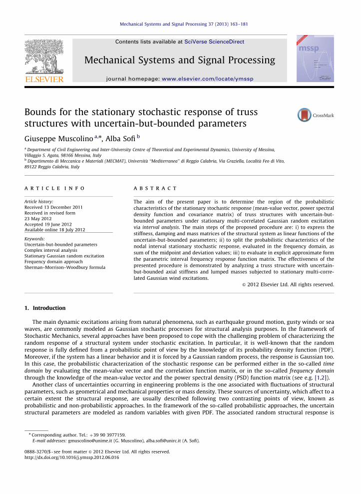
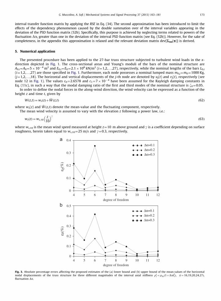
Fig. 2. Modulus of the element H11 of the FRF matrix of the truss structure with: (a) uncertain-but-bounded axial stiffness of five bars

rIi ¼ r0,ið1þDae

Ii Þ for¼ e

Ii ¼ 1, ði¼ 16,19,20,24,27Þ and (b) uncertain-but-bounded lumped masses associated with five horizontal nodal displacements

mIi ¼m0ð1þDae

Ii Þ for e

Ii ¼ 1, ði¼ 4,7,10,11,12Þ.

1 2

3.0

m

3.0

m

3.0 m

1 7

8

9

3.0 m

3.0

m

2

3 6

4

5

10 11

12 13

14 15

16 17

18 19

20 21

22 23

24 25

26 27

5 6

8 9

3

11 12

x

z

v12(t)

u12(t)

Fx,7(z7, t) 7

Fx,4(z4, t) 4

Fx,10(z10, t)10

wind

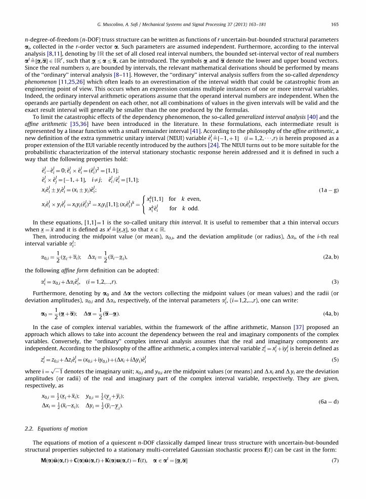
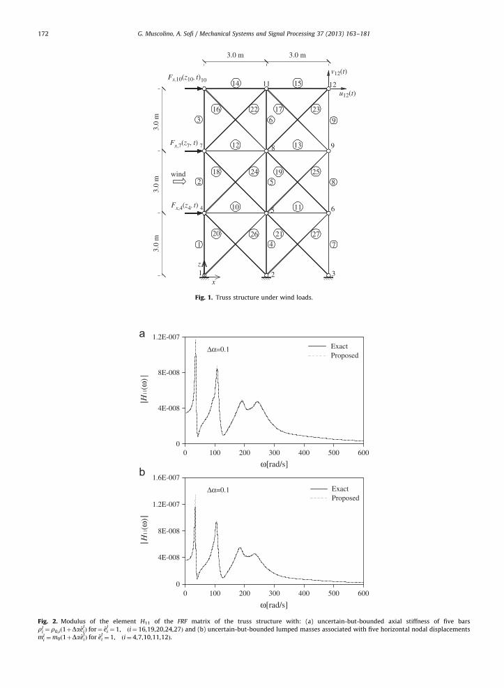
Fig. 1. Truss structure under wind loads.



interval transfer function matrix by applying the RSE in Eq. (34). The second approximation has been introduced to limit theeffects of the dependency phenomenon caused by the double summation over of the interval variables appearing in thedeviation of the PSD function matrix (52b). Specifically, this purpose is achieved by neglecting terms related to powers of thefluctuation Dai greater than one in the deviation of the interval PSD function matrix (see Eq. (52b)). However, for the sake ofcompleteness, in the appendix this approximation is relaxed and the relevant deviation matrix dev{Ruu(a)} is derived.

5. Numerical application

The presented procedure has been applied to the 27-bar truss structure subjected to turbulent wind loads in the x-direction depicted in Fig. 1. The cross-sectional areas and Young’s moduli of the bars of the nominal structure areA0,i¼A0¼5�10�4 m2 and E0,i¼E0¼2.1�108 kN/m2 (i¼1,2,y,27), respectively, while the nominal lengths of the bars L0,i

(i¼1,2,y,27) are those specified in Fig. 1. Furthermore, each node possesses a nominal lumped mass m0,j¼m0¼1000 Kg,(j¼1,2,y,18). The horizontal and vertical displacements of the j-th node are denoted by uj(t) and vj(t), respectively (seenode 12 in Fig. 1). The values c0¼2.6578 and c1¼7�10�4 have been assumed for the Rayleigh damping constants inEq. (11c), in such a way that the modal damping ratio of the first and third modes of the nominal structure is z0¼0.05.

In order to define the nodal forces in the along-wind direction, the wind velocity can be expressed as a function of theheight z and time t, given by

Wðz,tÞ ¼wsðzÞþ ~W ðz,tÞ ð62Þ

where ws(z) and ~W ðz,tÞ denote the mean-value and the fluctuating component, respectively.The mean wind velocity is assumed to vary with the elevation z following a power law, i.e.:

wsðzÞ ¼ws,10z

10

� gð63Þ

where ws,10 is the mean wind speed measured at height z¼10 m above ground and g is a coefficient depending on surfaceroughness, herein taken equal to ws,10¼25 m/s and g¼0.3, respectively.

degree of freedom

degree of freedom

0

0.1

0.2

0.3

0.4

εμ(%

)

Δα=0.1Δα=0.2Δα=0.3

Δα=0.1Δα=0.2Δα=0.3

4 5 6 7 8 9 10 11 12

4 5 6 7 8 9 10 11 120

0.1

0.2

0.3

0.4

0.5

εμ(%

)

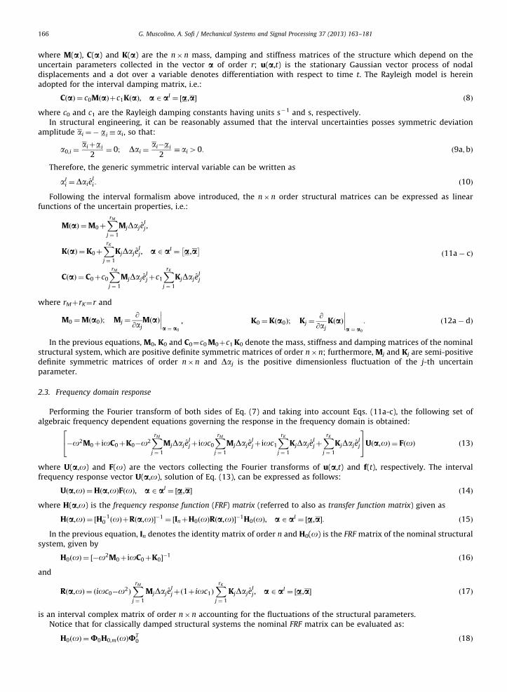
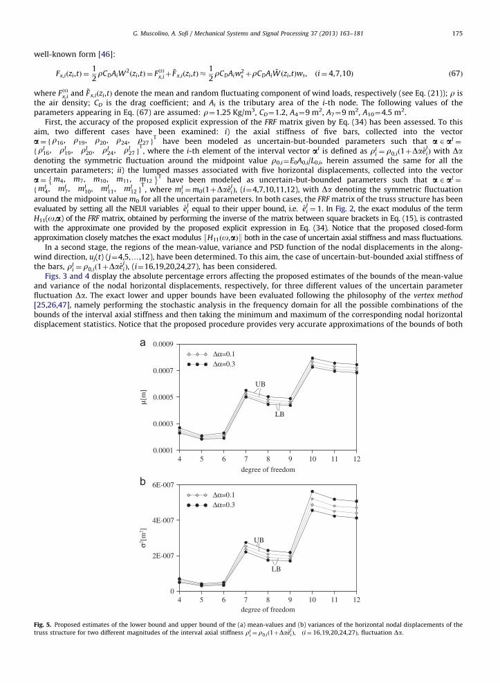
Fig. 3. Absolute percentage errors affecting the proposed estimates of the (a) lower bound and (b) upper bound of the mean-values of the horizontal

nodal displacements of the truss structure for three different magnitudes of the interval axial stiffness rIi ¼ r0,ið1þDae

Ii Þ, ði¼ 16,19,20,24,27Þ,

fluctuation Da.


The fluctuating component ~W ðz,tÞ, due to the turbulence in the flowing wind, is modeled as a zero-mean stationaryGaussian random field, fully described from a probabilistic point of view by the PSD function S ~W ~W ðoÞ. In the present study,the one-sided power spectrum proposed by Davenport [45] is assumed:

S ~W ~W ðoÞ ¼ 4K0w2s,10

w2

o 1þw2 �4=3

ð64Þ

where K0 is the non-dimensional roughness coefficient, herein set equal to K0¼0.03, and w¼b1o/(pvs,10) withb1¼600 m.

The wind velocity fluctuations at the p¼3 wind-exposed nodes (4, 7, 10) of the truss structure (see Fig. 1), located atdifferent heights zi, are correlated and can be collected into a vector ~WðtÞ representing a p-variate zero-mean stationaryGaussian random process. In view of the Gaussianity, the probabilistic characterization of ~WðtÞ is ensured by theknowledge of the PSD function matrix S ~W ~W ðoÞ. If the imaginary part (q-spectrum) [46] is neglected, the cross-PSDcomponents of S ~W ~W ðoÞ can be expressed as follows:

S ~W i~W jðzi,zj;oÞ ¼ S ~W ~W ðoÞf ijðoÞ ð65Þ

where fij(o) is the so-called coherence function, defined as

f ijðoÞ ¼ Exp �oj j

ffiffiffiffiffiffiffiffiffiffiffiffiffiffiffiffiffiffiffiffiffiffiC2

z ðzi�zjÞ2

qp wsðziÞþwsðzjÞ� �

8<:

9=; ð66Þ

with Cz denoting an appropriate decay coefficient to be determined experimentally, herein set equal to Cz¼10.Neglecting the contribution of the nodal velocities of the structure and the square of the fluctuating component of wind

speed, the x-direction wind forces exerted on the wind-exposed nodes (4, 7, 10) of the truss can be expressed in the

degree of freedom

0

1

2

3

4Δα=0.1Δα=0.2Δα=0.3

4 5 6 7 8 9 10 11 12

4 5 6 7 8 9 10 11 12

degree of freedom

0

0.4

0.8

1.2

1.6Δα=0.1Δα=0.2Δα=0.3

Fig. 4. Absolute percentage errors affecting the proposed estimates of the (a) lower bound and (b) upper bound of the variances of the horizontal nodal

displacements of the truss structure for three different magnitudes of the interval axial stiffness rIi ¼ r0,ið1þDae

Ii Þ, ði¼ 16,19,20,24,27Þ, fluctuation Da.


well-known form [46]:

Fx,iðzi,tÞ ¼1

2rCDAiW

2ðzi,tÞ ¼ FðsÞx,iþ

~F x,iðzi,tÞ �1

2rCDAiw

2s þrCDAi

~W ðzi,tÞws, ði¼ 4,7,10Þ ð67Þ

where FðsÞx,i and ~F x,iðzi,tÞ denote the mean and random fluctuating component of wind loads, respectively (see Eq. (21)); r isthe air density; CD is the drag coefficient; and Ai is the tributary area of the i-th node. The following values of theparameters appearing in Eq. (67) are assumed: r¼1.25 Kg/m3, CD¼1.2, A4¼9 m2, A7¼9 m2, A10¼4.5 m2.

First, the accuracy of the proposed explicit expression of the FRF matrix given by Eq. (34) has been assessed. To thisaim, two different cases have been examined: i) the axial stiffness of five bars, collected into the vectora¼ fr16, r19, r20, r24, r27 g

Thave been modeled as uncertain-but-bounded parameters such that a 2 aI ¼

frI16, rI

19, rI20, rI

24, rI27 g

T, where the i-th element of the interval vector aI is defined as rI

i ¼ r0,ið1þDaeIiÞ with Da

denoting the symmetric fluctuation around the midpoint value r0,i¼E0A0,i/L0,i, herein assumed the same for all theuncertain parameters; ii) the lumped masses associated with five horizontal displacements, collected into the vectora¼ m4, m7, m10, m11, m12

� �Thave been modeled as uncertain-but-bounded parameters such that a 2 aI ¼

fmI4, mI

7, mI10, mI

11, mI12 g

T, where mI

i ¼m0ð1þDaeIiÞ, (i¼4,7,10,11,12), with Da denoting the symmetric fluctuation

around the midpoint value m0 for all the uncertain parameters. In both cases, the FRF matrix of the truss structure has beenevaluated by setting all the NEUI variables e

Ii equal to their upper bound, i.e. e

Ii ¼ 1. In Fig. 2, the exact modulus of the term

H11(o,a) of the FRF matrix, obtained by performing the inverse of the matrix between square brackets in Eq. (15), is contrastedwith the approximate one provided by the proposed explicit expression in Eq. (34). Notice that the proposed closed-formapproximation closely matches the exact modulus :H11ðo,aÞ: both in the case of uncertain axial stiffness and mass fluctuations.

In a second stage, the regions of the mean-value, variance and PSD function of the nodal displacements in the along-wind direction, uj(t) (j¼4,5,y,12), have been determined. To this aim, the case of uncertain-but-bounded axial stiffness ofthe bars, rI

i ¼ r0,ið1þDaeIiÞ, (i¼16,19,20,24,27), has been considered.

Figs. 3 and 4 display the absolute percentage errors affecting the proposed estimates of the bounds of the mean-valueand variance of the nodal horizontal displacements, respectively, for three different values of the uncertain parameterfluctuation Da. The exact lower and upper bounds have been evaluated following the philosophy of the vertex method

[25,26,47], namely performing the stochastic analysis in the frequency domain for all the possible combinations of thebounds of the interval axial stiffness and then taking the minimum and maximum of the corresponding nodal horizontaldisplacement statistics. Notice that the proposed procedure provides very accurate approximations of the bounds of both

degree of freedom

0.0001

0.0003

0.0005

0.0007

0.0009

μ[m

]

Δα=0.1Δα=0.3

UB

LB

4 5 6 7 8 9 10 11 12

4 5 6 7 8 9 10 11 12degree of freedom

0

2E-007

4E-007

6E-007

σ2 [m2 ]

Δα=0.1Δα=0.3

UB

LB

Fig. 5. Proposed estimates of the lower bound and upper bound of the (a) mean-values and (b) variances of the horizontal nodal displacements of the

truss structure for two different magnitudes of the interval axial stiffness rIi ¼ r0,ið1þDae

Ii Þ, ði¼ 16,19,20,24,27Þ, fluctuation Da.

0

4E-008

8E-008

1.2E-007

1.6E-007

Su4(

ω)

[m2 s

]Su

10 (

ω)

[m2 s

]

UB (Exact)LB (Exact)UB (Proposed)LB (Proposed)Midpoint (Proposed)

Δα=0.3

0 0.4 0.8 1.2

0 0.4 0.8 1.2ω[rad/s]

ω[rad/s]

0

4E-007

8E-007

1.2E-006UB (Exact)LB (Exact)UB (Proposed)LB (Proposed)Midpoint (Proposed)

Δα=0.3

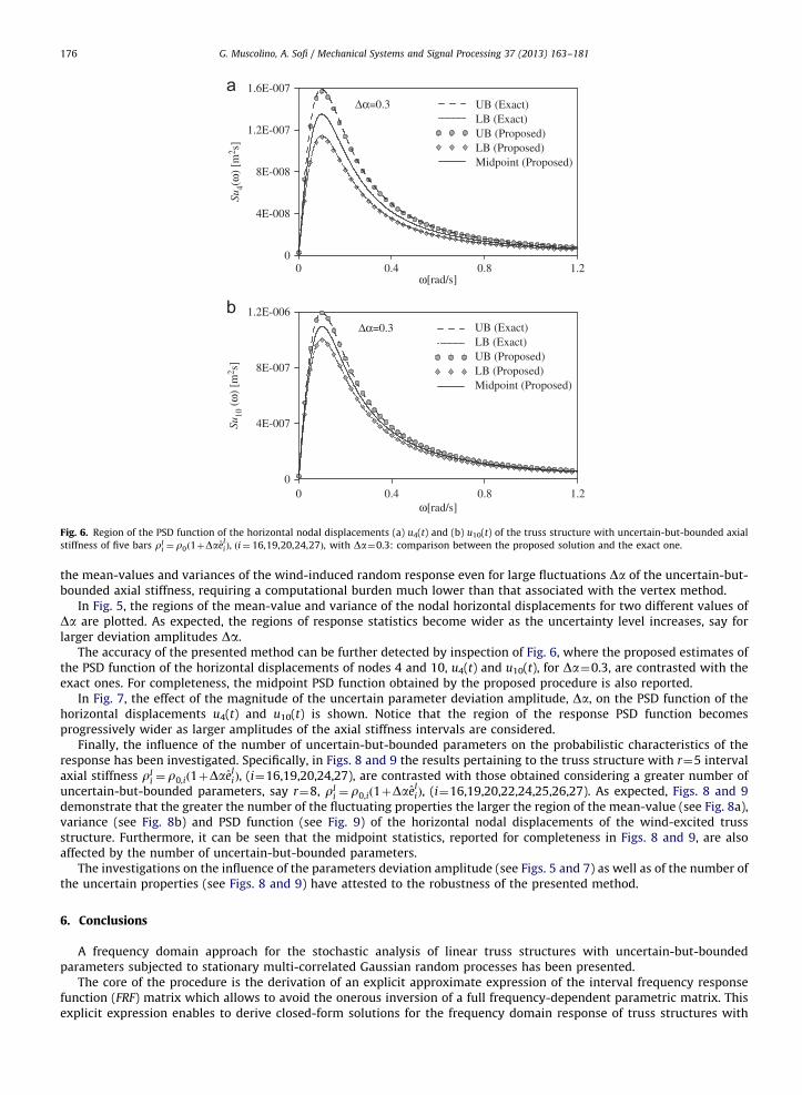
Fig. 6. Region of the PSD function of the horizontal nodal displacements (a) u4(t) and (b) u10(t) of the truss structure with uncertain-but-bounded axial

stiffness of five bars rIi ¼ r0ð1þDae

Ii Þ, ði¼ 16,19,20,24,27Þ, with Da¼0.3: comparison between the proposed solution and the exact one.


the mean-values and variances of the wind-induced random response even for large fluctuations Da of the uncertain-but-bounded axial stiffness, requiring a computational burden much lower than that associated with the vertex method.

In Fig. 5, the regions of the mean-value and variance of the nodal horizontal displacements for two different values ofDa are plotted. As expected, the regions of response statistics become wider as the uncertainty level increases, say forlarger deviation amplitudes Da.

The accuracy of the presented method can be further detected by inspection of Fig. 6, where the proposed estimates ofthe PSD function of the horizontal displacements of nodes 4 and 10, u4(t) and u10(t), for Da¼0.3, are contrasted with theexact ones. For completeness, the midpoint PSD function obtained by the proposed procedure is also reported.

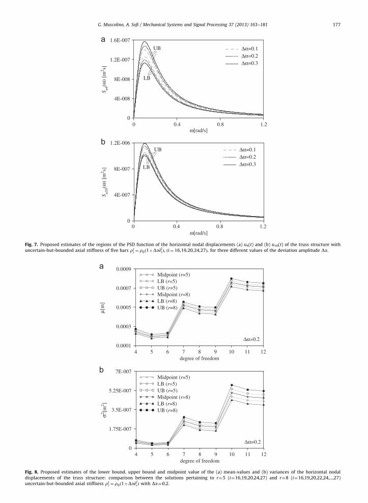
In Fig. 7, the effect of the magnitude of the uncertain parameter deviation amplitude, Da, on the PSD function of thehorizontal displacements u4(t) and u10(t) is shown. Notice that the region of the response PSD function becomesprogressively wider as larger amplitudes of the axial stiffness intervals are considered.

Finally, the influence of the number of uncertain-but-bounded parameters on the probabilistic characteristics of theresponse has been investigated. Specifically, in Figs. 8 and 9 the results pertaining to the truss structure with r¼5 intervalaxial stiffness rI

i ¼ r0,ið1þDaeIiÞ, (i¼16,19,20,24,27), are contrasted with those obtained considering a greater number of

uncertain-but-bounded parameters, say r¼8, rIi ¼ r0,ið1þDae

IiÞ, (i¼16,19,20,22,24,25,26,27). As expected, Figs. 8 and 9

demonstrate that the greater the number of the fluctuating properties the larger the region of the mean-value (see Fig. 8a),variance (see Fig. 8b) and PSD function (see Fig. 9) of the horizontal nodal displacements of the wind-excited trussstructure. Furthermore, it can be seen that the midpoint statistics, reported for completeness in Figs. 8 and 9, are alsoaffected by the number of uncertain-but-bounded parameters.

The investigations on the influence of the parameters deviation amplitude (see Figs. 5 and 7) as well as of the number ofthe uncertain properties (see Figs. 8 and 9) have attested to the robustness of the presented method.

6. Conclusions

A frequency domain approach for the stochastic analysis of linear truss structures with uncertain-but-boundedparameters subjected to stationary multi-correlated Gaussian random processes has been presented.

The core of the procedure is the derivation of an explicit approximate expression of the interval frequency responsefunction (FRF) matrix which allows to avoid the onerous inversion of a full frequency-dependent parametric matrix. Thisexplicit expression enables to derive closed-form solutions for the frequency domain response of truss structures with

0

4E-008

8E-008

1.2E-007

1.6E-007

Δα=0.1Δα=0.2Δα=0.3

UB

LB

0 0.4 0.8 1.2

0 0.4 0.8 1.2ω[rad/s]

ω[rad/s]

0

4E-007

8E-007

1.2E-006

S u4(ω

) [m

2 s]

S u10

(ω) [

m2 s]

Δα=0.1Δα=0.2Δα=0.3

UB

LB

Fig. 7. Proposed estimates of the regions of the PSD function of the horizontal nodal displacements (a) u4(t) and (b) u10(t) of the truss structure with

uncertain-but-bounded axial stiffness of five bars rIi ¼ r0ð1þDae

Ii Þ, ði¼ 16,19,20,24,27Þ, for three different values of the deviation amplitude Da.

degree of freedom

0.0001

0.0003

0.0005

0.0007

0.0009

μ[m

]

Midpoint (r=5)LB (r=5)UB (r=5)Midpoint (r=8)LB (r=8)UB (r=8)

Δα=0.2

4 5 6 7 8 9 10 11 12

4 5 6 7 8 9 10 11 12degree of freedom

0

1.75E-007

3.5E-007

5.25E-007

7E-007

σ2 [m2 ]


Δα=0.2

Fig. 8. Proposed estimates of the lower bound, upper bound and midpoint value of the (a) mean-values and (b) variances of the horizontal nodal

displacements of the truss structure: comparison between the solutions pertaining to r¼5 (i¼16,19,20,24,27) and r¼8 (i¼16,19,20,22,24,...,27)

uncertain-but-bounded axial stiffness rIi ¼ r0ð1þDae

Ii Þ with Da¼0.2.


ω[rad/s]

ω[rad/s]

0

5.5E-008

1.1E-007

1.65E-007Midpoint (r=5)LB (r=5)UB (r=5)Midpoint (r=8)LB (r=8)UB (r=8)


Δα=0.2

0 0.4 0.8 1.2

0 0.4 0.8 1.20

4.1E-007

8.2E-007

1.23E-006

S u10

(ω) [

m2 s]

S u

4(ω) [

m2 s]

Δα=0.2

Fig. 9. Proposed estimates of the lower bound, upper bound and midpoint value of the PSD function of the horizontal nodal displacements (a) u4(t) and

(b) u10(t) of the truss structure: comparison between the solutions pertaining to r¼5 (i¼16,19,20,24,27) and r¼8 (i¼16,19,20,22,24,...,27) uncertain-but-

bounded axial stiffness rIi ¼r0ð1þDae

Ii Þ with Da¼0.2.


fluctuating properties which may be exploited for performing sensitivity analysis, reliability analysis, optimization, etc.A notable feature of the proposed explicit expression of the FRF matrix is that it holds whatever model is adopted torepresent the uncertain properties. This implies that potential applications also include the analysis of truss structureswith fluctuating parameters modeled within the framework of classical probability theory. Another remark concerns theapplicability of the approximate FRF matrix in conjunction with interval finite element models to address the stochasticanalysis of any kind of structure. Indeed, the proposed closed-form expression of the FRF matrix just requires to expressthe mass, stiffness and damping matrices as sum of the midpoint value plus a deviation given as the superposition of rank-one matrices.

Following the philosophy of the so-called affine arithmetic, an improvement of the ‘‘ordinary’’ complex interval analysis,based on the introduction of a particular unitary interval variable, has been proposed for determining the region of theprobabilistic characteristics of the stationary stochastic response in the frequency domain.

For validation purposes, a truss structure subjected to stationary multi-correlated Gaussian wind excitationshas been analyzed. Both mass and axial stiffness fluctuations have been considered and the accuracy of the approximateexplicit FRF matrix has been assessed. Moreover, appropriate comparisons with the exact bounds obtained followingthe philosophy of the vertex method have demonstrated that the presented procedure provides very accurate estimatesof the region of the interval mean-values, variances and power spectral density functions of the stationary responseeven for large parameter fluctuations. Therefore, the proposed improvement of the ‘‘ordinary’’ complex interval analysishas proved able to eliminate the overestimation of the interval response width due to the so-called dependency

phenomenon.

Acknowledgments

The authors are grateful to the two anonymous reviewers for their valuable suggestions on an earlier version ofthis paper.


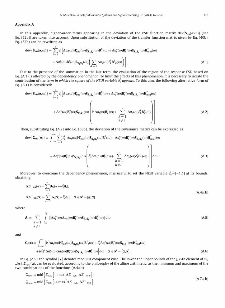
Appendix A

In this appendix, higher-order terms appearing in the deviation of the PSD function matrix dev{Suu(a,o)} (seeEq. (52b)) are taken into account. Upon substitution of the deviation of the transfer function matrix given by Eq. (40b),Eq. (52b) can be rewritten as


¼Xr

i ¼ 1

eIi DaiðoÞHn

midðoÞS ~Xf~XfðoÞBT

iðoÞþDan

i ðoÞBn


midðoÞh

þDan

i ðoÞBn

i ðoÞS ~Xf~XfðoÞ

Xr

k ¼ 1

DakðoÞeIkBT

kðoÞ !#

: ðA:1Þ

Due to the presence of the summation in the last term, the evaluation of the region of the response PSD based onEq. (A.1) is affected by the dependency phenomenon. To limit the effects of this phenomenon, it is necessary to isolate thecontribution of the term in which the square of the NEUI variable e

Ii appears. To this aim, the following alternative form of

Eq. (A.1) is considered:


¼Xr

i ¼ 1

eIi DaiðoÞHn


i ðoÞþDan

i ðoÞBn


midðoÞh

þDan

i ðoÞBn

i ðoÞS ~Xf~XfðoÞ e

IiDaiðoÞBT

i ðoÞþXr

k¼ 1kai

DakðoÞeIkBT

k ðoÞ

0BBBBBB@

1CCCCCCA

37777775: ðA:2Þ

Then, substituting Eq. (A.2) into Eq. (58b), the deviation of the covariance matrix can be expressed as

dev RuuðaÞ� �

¼

Z 1�1

Xr

i ¼ 1

eIi DaiðoÞHn


i ðoÞþDan

i ðoÞBn


midðoÞh

þDan

i ðoÞBn

i ðoÞS ~Xf~XfðoÞ e

IiDaiðoÞBT

i ðoÞþXr

k¼ 1kai

DakðoÞeIkBT

k ðoÞ

0BBBBBB@

1CCCCCCA

37777775

do: ðA:3Þ

Moreover, to overcome the dependency phenomenon, it is useful to set the NEUI variable eIk9½�1,1� at its bounds,

obtaining:

DR�uuðaÞ ¼Xr

i ¼ 1

½GiðaÞ�eIiAi�;

DRþ uuðaÞ ¼Xr

i ¼ 1

½GiðaÞþ eIiAi�, a 2 aI ¼ ½a,a�

ðA:4a;bÞ

where

Ai ¼Xr

k¼ 1kai

Z1�1

:Dan

i ðoÞDakðoÞBn

i ðoÞS ~Xf~XfðoÞBT

k ðoÞ:do ðA:5Þ

and

GiðaÞ ¼Z 1�1

eIiDaiðoÞHn


iðoÞþ eIiDan

i ðoÞBn


midðoÞh

þðeIiÞ

2Dan

i ðoÞDaiðoÞBn

i ðoÞS ~Xf~XfðoÞBT

i ðoÞido a 2 aI ¼ a,a

� �: ðA:6Þ

In Eq. (A.5), the symbol :�: denotes modulus component wise. The lower and upper bounds of the j, ‘-th element of Ru

u(a), Suju‘ ðaÞ, can be evaluated, according to the philosophy of the affine arithmetic, as the minimum and maximum of thetwo combinations of the functions (A.4a,b)

Suju‘ ¼mid Suju‘

n o�max DS�uju‘ ,DS

þuju‘

h i;

Suju‘¼mid Suju‘

n oþmax DS�uju‘ ,DS

þuju‘

h i ðA:7a;bÞ


where DS�uju‘ and DSþ uju‘ are the j,‘-th elements of the matrices DR�uu and DRþ uu obtained, respectively, as

DR�uu ¼Xr

i ¼ 1

G�i þAi

�� ;DRþ uu ¼

Xr

i ¼ 1

Gþi þAi

�� ðA:8a;bÞ

where G�i and Gþi are obtained from the matrix Gi(a) defined in Eq. (A.6) by setting the NEUI variable eIi ¼ �1,þ1½ � at its

bounds, while the symbol 9�9 denotes absolute component wise.

References

[1] L.D. Lutes, S. Sarkani, Stochastic Analysis of Structural and Mechanical Vibrations, Prentice-Hall, Upper Sudale River, 1997.[2] J. Li, J.B. Chen, Stochastic Dynamics of Structures, John Wiley & Sons, Singapore, 2009.[3] M. Kleiber, H.D. Hien, The Stochastic Finite Element Method: Basic Perturbation Technique and Computer Implementation, John-Wiley & Sons,

Chichester, UK, 1992.[4] R.G. Ghanem, P.D. Spanos, Stochastic Finite Elements: A Spectral Approach, Springer-Verlag, New York, USA, 1991.[5] M. Di Paola, A. Pirrotta, M. Zingales, Stochastic dynamics of linear elastic trusses in presence of structural uncertainties (virtual distortion approach),

Probab. Eng. Mech. 19 (2004) 41–51.[6] M. Di Paola, Probabilistic analysis of truss structures with uncertain parameters (virtual distorsion method approach), Probab. Eng. Mech. 19 (2004)

321–329.[7] I. Elishakoff, M. Ohsaki, Optimization and Anti-Optimization of Structures under Uncertainties, Imperial College Press, London, 2010.[8] R.E. Moore, Interval Analysis, Prentice-Hall, Englewood Cliffs, 1966.[9] G. Alefeld, J. Herzberger, Introduction to Interval Computations, Academic Press, New York, 1983.

[10] A. Neumaier, Interval Methods for Systems of Equations, Cambridge University Press, Cambridge, UK, 1990.[11] R.E. Moore, R.B. Kearfott, M.J. Cloud, Introduction to Interval Analysis, SIAM, Philadelphia, USA, 2009.[12] Z.S. Liu, S.H. Chen, W.Z. Han, Solving the extremum of static response for structural systems with unknown-but-bounded parameters, Comput.

Struct. 50 (1994) 557–561.[13] Z.P. Qiu, S.H. Chen, D. Song, The displacement bound estimation for structures with an interval description of uncertain parameters, Commun.

Numer. Methods Eng. 12 (1996) 1–11.[14] Z.P. Qiu, I. Elishakoff, Anti-optimization of structures with large uncertain-but-non-random parameters via interval analysis, Comput. Methods Appl.

Mech. Eng. 152 (1998) 361–372.[15] S. McWilliam, Anti-optimization of uncertain structures using interval analysis, Comput. Struct. 79 (2001) 421–430.[16] S.H. Chen, H.D. Lian, X.W. Yang, Interval static displacement analysis for structures with interval parameters, Int. J. Numer. Methods Eng. 53 (2002)

393–407.[17] Z.P. Qiu, X.J. Wang, Comparison of dynamic response of structures with uncertain-but-bounded parameters using nonprobabilistic interval analysis

method and probabilistic approach, Int. J. Solids Struct. 40 (2003) 5423–5439.[18] Z.P. Qiu, X.J. Wang, Parameter perturbation method for dynamic responses of structures with uncertain-but-bounded parameters based on interval

analysis, Int. J. Solids Struct. 4 (2005) 4958–4970.[19] X.M. Zhang, H. Ding, S.H. Chen, Interval finite element method for dynamic response of closed-loop system with uncertain parameters, Int. J. Numer.

Methods Eng. 70 (2007) 543–562.[20] G. Muscolino, A. Sofi, Stochastic response of structures with uncertain-but-bounded parameters, in: Proceedings of the IMECE 2009, November

13–19, Lake Buena Vista, Florida, USA, 2009.[21] G. Muscolino, A. Sofi, Response statistics of linear structures with uncertain-but-bounded parameters under gaussian stochastic input, Int. J. Struct.

Stability Dyn. 11 (2011) 1–30.[22] G. Muscolino, A. Sofi, Response of structural systems with uncertain-but-bounded parameters under stationary stochastic input via interval analysis,

in: G. De Roeck, G. Degrande, G. Lombaert, G. Muller, (Eds.), Proceedings of the 8th International Conference on Structural Dynamics, EURODYN2011, Leuven, Belgium, 4–6 July 2011, pp. 3016–3023, 978-90-760-1931-4.

[23] G. Muscolino, A. Sofi, Stochastic analysis of structures with uncertain-but-bounded parameters, in: G. Deodatis, P.D. Spanos (Eds.), ComputationalStochastic Mechanics, Research Publishing, Singapore, 2011, pp. 415–427.

[24] G. Muscolino, A. Sofi, Stochastic analysis of structures with uncertain-but-bounded parameters via improved interval analysis, Probab. Eng. Mech.28 (2012) 152–163.

[25] R.L. Muhanna, R.L. Mullen, Uncertainty in mechanics problems-interval-based approach, J. Eng. Mech.—ASCE 127 (2001) 557–566.[26] D. Moens, D. Vandepitte, A survey of non-probabilistic uncertainty treatment in finite element analysis, Comput. Methods Appl. Mech. Eng. 194

(2005) 1527–1555.[27] U. Koyluoglu, I. Elishakoff, A comparison of stochastic and interval finite elements applied to shear frames with uncertain stiffness properties,

Comput. Struct. 67 (1998) 91–98.[28] S.-H. Chen, X.-W. Yang, Interval finite element method for beam structures, Finite Elem. Anal. Des. 34 (2000) 75–88.[29] W. Gao, Interval finite element analysis using interval factor method, Comput. Mech. 39 (2007) 709–717.[30] O. Dessombz, F. Thouverez, J.-P. Laıne, L. Jezequel, Analysis of mechanical systems using interval computations applied to finite element methods,

J. Sound Vib. 239 (5) (2001) 949–968.[31] M.V. Rama Rao, A. Pownuk, S. Vandewalle, D. Moens, Transient response of structures with uncertain structural parameters, Struct. Saf. 32 (2010)

449–460.[32] D. Moens, M. Hanss, Non-probabilistic finite element analysis for parametric uncertainty treatment in applied mechanics: recent advances, Finite

Elem. Anal. Des. 47 (2011) 4–16.[33] D. Degrauwe, G. Lombaert, G. De Roeck, Improving interval analysis in finite element calculations by means of affine arithmetic, Comput. Struct. 88

(2010) 247–254.[34] R. Bellman, Introduction to Matrix Analysis, McGraw-Hill, New York, USA, 1974.[35] J.L.D. Comba, J. Stolfi, Affine arithmetic and its applications to computer graphics, Anais do VI Simposio Brasileiro de Computaao Grafica e

Processamento de Imagens (SIBGRAPI’93’’, Recife (Brazil), October, 9–18, 1993.[36] J. Stolfi, L.H. De Figueiredo, An introduction to affine arithmetic, TEMA Tend. Mat. Apl. Comput. 4 (2003) 297–312.[37] G. Manson, Calculating frequency response functions for uncertain systems using complex affine analysis, J. Sound Vib. 288 (2005) 487–521.[38] G. Muscolino, A. Sofi, R. Santoro. Frequency response functions of discretized structural systems with uncertain parameters, in: Proceedings of the

5th International Conference on Reliable Engineering Computing (REC2012) Practical Applications and Practical Challenges, June 13–15, Brno, CzechRepublic, 2012.


[39] N. Impollonia, G. Muscolino, Interval analysis of structures with uncertain-but-bounded axial stiffness, Comput. Methods Appl. Mech. Eng. 220(2011) 1945–1962.

[40] E.R. Hansen, A generalized interval arithmetic, in: K. Nicket (Ed.), Interval Mathematics, Lecture Notes in Computer Science, 29, 1975, pp. 7–18.[41] N.S. Nedialkov, V. Kreinovich, S.A. Starks, Interval arithmetic, affine arithmetic, Taylor series methods: why, what next? Numer. Algorithms 37

(2004) 325–336.[42] J. Sherman, W.J. Morrison, Adjustment of an inverse matrix corresponding to a change in one element of a given matrix, Ann. Math. Stat. 21 (1)

(1950) 124–127.[43] M. Woodbury, Inverting Modified Matrices. Memorandum Report 42. Statistical Research Group, Princeton University, Princeton, NJ, 1950.[44] J. Rohn, Inverse interval matrix, SIAM J. Numer. Anal. 30 (1993) 864–870.[45] A.G. Davenport, The spectrum of horizontal gustiness near the ground in high winds, Q. J. R. Meteorol. Soc. 87 (1961) 194–211.[46] E. Simiu, R. Scanlan, Wind Effects on Structures, John Wiley & Sons, New York, 1996.[47] Z.P. Qiu, X.J. Wang, S.H. Chen, Exact bounds for the static response set of structures with uncertain-but-bounded parameters, Int. J. Solids Struct. 43

(2006) 6574–6593.

Date post:	30-Dec-2016
Category:	Documents
Upload:	alba
View:	213 times
Download:	1 times

Bounds for the stationary stochastic response of truss structures with uncertain-but-bounded...

Documents