Branching Processes

Linda J. S. AllenTexas Tech University

The study of branching processes began in the 1840s with Irenee-Jules Bienayme, a prob-

abilist and statistician, and was advanced in the 1870s with the work of Reverend Henry

William Watson, a clergyman and mathematician, and Francis Galton, a biometrician. In

1873, Galton sent a problem to the Educational Times regarding the survival of family names.

When he did not receive a satisfactory answer, he consulted Watson, who rephrased the prob-

lem in terms of generating functions. The simplest and most frequently applied branching

process is named after Galton and Watson, a type of discrete-time Markov chain. Branching

processes fit under the general heading of stochastic processes. The methods employed in

branching processes allow questions about extinction and survival in ecology and evolution-

ary biology to be addressed. For example, suppose we are interested in family names, as in

Galton’s original problem, or in the spread of a potentially lethal mutant gene that arises in

a population, or in the success of an invasive species. Given information about the number

of offspring produced by an individual per generation, branching process theory can address

questions about the survival of a family name or a mutant gene or an invasive species. Other

questions that can be addressed with branching processes relate to the rate of population

growth in a stable versus a highly variable environment.

Some background in probability theory is required to apply branching process theory.

We present some of this background in the next section. Then we discuss single-type and

multi-type Galton-Watson branching processes, and extensions to random environments that

will address questions about population survival and growth.

1

I. Background

The fundamental tools required for studying branching processes are generating functions. As

the name implies, a generating function is a function that “generates” information about the

process. For example, a probability generating function is used to calculate the probabilities

associated with the process, whereas a moment generating function is used to calculate the

moments, such as the mean and variance. We introduce some notation and define some terms

in probability theory.

Let X be a discrete random variable taking values in the set 0, 1, 2, . . . with associated

probabilities,

pj = ProbX = j, j = 0, 1, 2, . . . ,

that sum to one,

p0 + p1 + p2 + · · · =∞∑j=0

pj = 1.

Let the expectation of u(X) be defined as

E(u(X)) = p0u(0) + p1u(1) + p2u(2) + · · · =∞∑j=0

pju(j).

If u(X) = X, then E(X) is the expectation of X or the mean of X,

E(X) = p1 + 2p2 + 3p3 + · · · =∞∑j=0

jpj = µ.

The summation reduces to a finite number of terms if, for example, pj = 0 for j > n.

With this notation, three generating functions important in the theory of branching pro-

cesses are defined. The probability generating function (pgf) of X is

P(s) = E(sX) = p0 + p1s+ p2s2 + · · · =

∞∑j=0

pjsj ,

where s is a real number. Evaluating P at s = 1 yields P(1) = 1. The moment generating

function (mgf) of X is

M(s) = E(esX) = p0 + p1es + p2e

2s + · · · =∞∑j=0

pjejs.

2

Evaluating M at s = 0 yields M(0) = 1. The cumulant generating function (cgf) of X

is the natural logarithm of the moment generating function,

K(s) = ln[M(s)].

Evaluating K at s = 0 yields K(0) = ln[M(0)] = ln 1 = 0.

As noted previously, the pgf generates the probabilities associated with the random vari-

able X. For example, if X is the random variable for the size of a population, then the

probability of population extinction p0 can be found by evaluating the pgf at s = 0:

P(0) = ProbX = 0 = p0.

Differentiation of P and evaluation at s = 0 equals p1, the probability that the population

size is one.

The mgf generates the moments of the random variable X. Differentiation of M and

evaluation at s = 0 yields the moments of X about the origin. For example, the mean of X

is the first derivative of M evaluated at s = 0. That is,

dM(s)ds

∣∣∣∣s=0

= M ′(0) =∞∑j=0

jpj = E(X).

The second moment is

E(X2) = M ′′(0).

The variance of X is σ2 = E[(X − µ)2]. Using properties of the expectation, the variance

can be expressed as σ2 = E(X2)− [E(X)]2. Written in terms of the mgf,

σ2 = M ′′(0)− [M ′(0)]2 =∞∑j=0

j2pj −

∞∑j=0

jpj

2

.

Formulas for the mean and variance of X can be computed from any one of the generating

functions by appropriate differentiation and evaluation at either s = 0 or s = 1. They are

defined as follows:

µ = P ′(1) = M ′(0) = K ′(0)

3

and

σ2 =

P ′′(1) + P ′(1)− [P ′(1)]2

M ′′(0)− [M ′(0)]2

K ′′(0)

.

The preceding expressions for the mean and variance will be applied in the following sections.

II. Galton-Watson branching process

Galton-Watson branching processes are discrete-time Markov chains, that is, collections

of discrete random variables, Xn∞n=0, where the time n = 0, 1, 2 . . . is also discrete. The

random variable Xn may represent the population size of animals, plants, cells, or genes at

time n or generation n. The term chain implies each of the random variables are discrete-

valued; their values come from the set of nonnegative integers 0, 1, 2, . . .. The name Markov

acknowledges the contributions of probabilist Andrei Markov to the theory of stochastic

processes. The Markov property means that the population size at time n + 1 is only

dependent on the population size at time n, and is not dependent on the size at earlier

times. In this way, the population size Xn at time n predicts the population size in the next

generation, Xn+1.

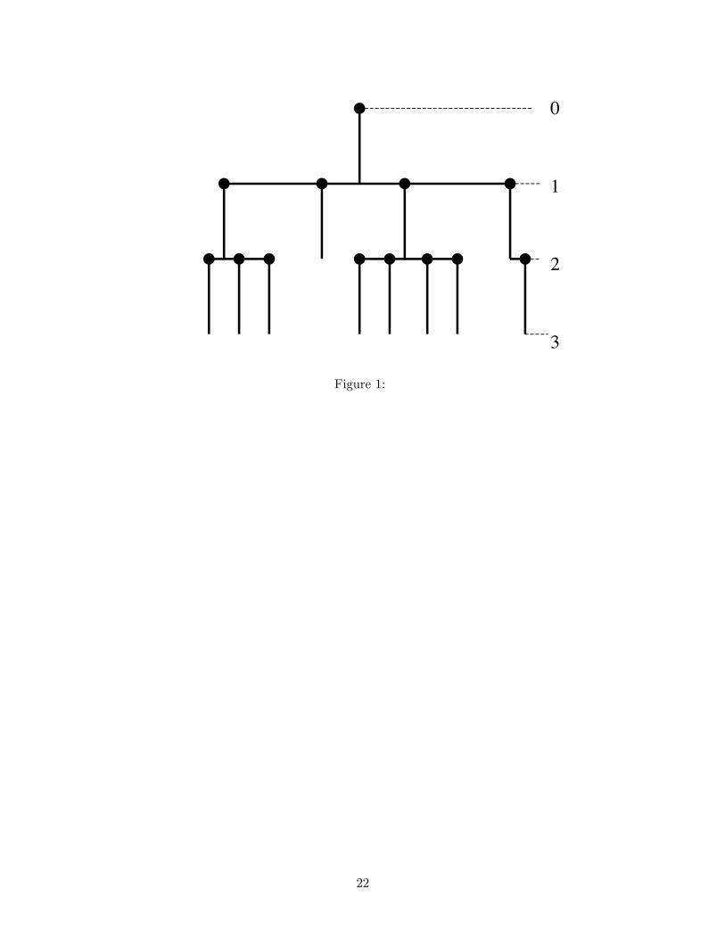
The graph in Fig. 1 illustrates what is referred to as a sample path or stochastic real-

ization of a branching process. Fig. 1 also shows why the name “branching” is appropriate

for this type of process. Beginning with an initial size of X0 = 1 such as one mutant gene, in

the next two generations, the number of mutant genes are X1 = 4 and X2 = 8, respectively.

The parent genes are replaced by progeny genes in subsequent generations. The graph illus-

trates just one of many possible sample paths for the number of mutant genes in generations

1 and 2. Associated with each parent population is an offspring distribution which specifies

the probability of the number of offspring produced in the next generation. The following

three assumptions define the Galton-Watson branching process more precisely.

Three important assumptions about the Markov process Xn∞n=0 define a single-type

Galton-Watson branching process (GWbp).

4

(i) Each individual in the population in generation n gives birth to Y offspring of the same

type in the next generation, where Y is a discrete random variable that takes values in

0, 1, 2 . . .. The offspring probabilities of Y are

pj = ProbY = j, j = 0, 1, 2, . . . .

(ii) Each individual in the population gives birth independently of all other individuals.

(iii) The same offspring distribution applies to all generations.

The expression “single-type” refers to the fact that all individuals are of one type such as the

same gender, same cell type, or same genotype or phenotype. The pgf of Xn will be denoted

as Pn and the pgf of Y as g.

If, in any generation n, the population size reaches zero, Xn = 0, then the process stops

and remains at zero, population extinction has occurred. The probability that the population

size is zero in generation n is found by setting s = 0 in the pgf,

ProbXn = 0 = Pn(0).

To obtain information about population extinction in generation n, it is necessary to

know the pgf in generation n, Pn(s). It can be shown that if the assumptions (i)-(iii) are

satisfied, then the pgf in generation n is just an n-fold composition of the pgf of the offspring

distribution g:

Pn(s) = g(g(· · · (g(s)) · · · )) = gn(s).

To indicate why this is true, note that if the initial population size is one, X0 = 1, then the

pgf of X0 is P0(s) = s. Then the pgf of X1 is just the offspring of the one individual from

the first generation, that is, X1 = Y so that P1(s) = g(s). In the case of two generations,

P2(s) = g(g(s)) = g2(s) so that the probability of population extinction after two generations

is simply P2(0) = g2(0). In general, the pgf in generation n is found by taking n compositions

of the offspring distribution g, as given above.

5

The preceding calculation assumed X0 = 1. The probability of extinction can be calcu-

lated when the initial population size is greater than one, X0 = N > 1. In this case, the pgf

of Xn is just the n-fold composition of g raised to the power N ,

Pn(s) = [gn(s)]N .

Then the probability of population extinction in generation n can be found by evaluating the

pgf at s = 0:

Pn(0) = [gn(0)]N .

In most cases, it is difficult to obtain an explicit simple expression for Pn(s) in generation

n. This is due to the fact that each time a composition is taken of another function, a more

complicated expression is obtained. Fortunately, it is still possible to obtain information about

the probability of population extinction after a long period of time (as n → ∞). Ultimate

extinction depends on the mean number of offspring produced by the parents. Recall that

the mean number of offspring can be computed from the pgf g(s) by taking its derivative and

evaluating at s = 1. We will denote the mean number of offspring as m,

m = g′(1) =∞∑j=1

jpj .

The following theorem is one of the most important results in GWbp: if the mean number

of offspring is less than or equal to one, m ≤ 1, then eventually the population dies out, but

if m > 1, the population has a chance of surviving. The probability of extinction depends on

the initial population size N and the offspring distribution g. The theorem also shows how

to calculate the probability of extinction if m > 1. A fixed point of g is calculated: a point q

such that g(q) = q and 0 < q < 1. Then the probability of extinction is qN .

Fundamental Theorem I: Let the initial population size of a GWbp be X0 = N ≥ 1

and let the mean number of offspring be m. Assume there is a positive probability of zero

offspring and a positive probability of more than two offspring.

6

If m ≤ 1, then the probability of ultimate extinction is one,

limn→∞

ProbXn = 0 = limn→∞

Pn(0) = 1.

If m > 1, then the probability of ultimate extinction is less than one,

limn→∞

ProbXn = 0 = limn→∞

Pn(0) = qN < 1,

where the value of q is the unique fixed point of g: g(q) = q and 0 < q < 1.

The GWbp is referred to as supercritical if m > 1, critical if m = 1, and subcritical if

m < 1. If the process is subcritical or critical, then the probability of extinction is certain. But

if the process is supercritical, then there is a positive probability, 1− qN , that the population

will survive. As the initial population size increases, the probability of survival also increases.

We apply the Fundamental Theorem 1 to the question of the survival of family names.

Example 1. Survival of family names. In 1931, Alfred Lotka assumed a zero-modified

geometric distribution to fit the offspring distribution of the 1920s American male population.

The theory of branching processes was used to address questions about survival of family

names. In the zero-modified geometric distribution, the probability that a father has j sons

is

pj = bpj−1, j = 1, 2, 3, . . .

and the probability that he has no sons is

p0 = 1− (p1 + p2 + · · · ) = 1−∞∑j=1

pj .

Lotka assumed b = 1/5, p = 3/5, and p0 = 1/2. Therefore, the probability of having no sons

is p0 = 1/2, the probability of having one son is p1 = 1/5, and so on. Then the offspring pgf

has the following form:

g(s) = p0 + p1s+ p2s2 + · · · = p0 +

∞∑j=1

bpj−1sj = p0 +bs

1− ps=

12

+s

5− 3s.

The mean number of offspring is m = g′(1) = 5/4 > 1. According to the Fundamental

Theorem I, in the supercritical case m > 1, there is a positive probability of survival, 1− qN ,

7

where N is the initial number of males. Applying the Fundamental Theorem I, the number q

is a fixed point of g, that is, a number q such that g(q) = q and 0 < q < 1. The fixed points

of g are found by solving the following equation:

12

+q

5− 3q= q.

There are two solutions, q = 1 and q = 5/6, but only one solution satisfies 0 < q < 1, namely

q = 5/6. It should be noted that q = 1 will always be one solution to g(q) = q due to one of

the properties of a pgf, g(1) = 1.

To address the question about the probability of survival of family names, it follows that

one male has a probability of 5/6 that his line of descent becomes extinct and a probability

of 1/6 that his descendants will continue forever.

The zero-modified geometric distribution is one of the few offspring distributions where an

explicit formula can be computed for the pgf of Xn, that is, the function Pn(s) = [gn(s)]N .

This particular case is referred to as the linear fractional case because of the form of the

generating function. For X0 = 1, the pgf of Xn for the linear fractional case is

Pn(s) =

(mnq − 1)s+ q(1−mn)

(mn − 1)s+ q −mn, if m 6= 1

[(n+ 1)p− 1]s− npnps− (n− 1)p− 1

, if m = 1,

where the value of q is a fixed point of g, g(q) = q. If m > 1, then q is chosen so that

0 < q < 1 and if m < 1, q is chosen so that q > 1.

Example 2. Probability of extinction. Applying the preceding formula to Lotka’s model

in Example 1, for X0 = 1, the probability of population extinction at the nth generation or

the probability that no sons are produced in generation n is found by evaluating the pgf at

s = 0:

Pn(0) =q(mn − 1)mn − q

, m > 1.

Substituting m = 5/4 and q = 5/6 into Pn(0), the probabilities of population extinction

in generation n can be easily calculated. They are graphed in Fig. 2. The probability of

8

extinction approaches q = 5/6 ≈ 0.83 for a single line of descent, X0 = 1. For three lines of

descent X0 = 3, q3 ≈ 0.58.

Formulas for the mean and variance of Xn depend on the mean and variance of the

offspring distribution, m and σ2. The expectation of Xn is

E(Xn) = mE(Xn−1) = mnE(X0)

and the variance is

E[(Xn − E(Xn))2

]=

mn−1(mn − 1)m− 1

σ2, m 6= 1

nσ2, m = 1.

In the subcritical case, m < 1, the mean population size of Xn decreases geometrically. In

the critical case, m = 1, the mean size is constant but the variance of the population size

Xn increases linearly, and in the supercritical case, m > 1, the mean and variance increase

geometrically. This is an interesting result when one considers that in the supercritical case,

there is a probability of extinction of qN . In the next example, branching processes are used

to study the survival of a mutant gene.

Example 3. Survival of a mutant gene. Suppose the population size is very large. A

new mutant gene appears in N individuals of the population; the remaining individuals in

the population do not carry the mutant gene. Individuals reproduce according to a branching

process and those individuals with a mutant gene have offspring that carry the mutant gene.

Suppose the mean number of offspring from parents with a mutant gene is m. If m ≤ 1,

then the line of descendants from the individuals with a mutant gene will eventually become

extinct with probability one. But suppose the mutant gene has a mean that is slightly greater

than 1,

m = 1 + ε, ε > 0,

there is a probability 1− qN that the subpopulation with the mutant gene will survive. The

value of q can be approximated from the cgf K(s) = lnM(s) using the fact that K(0) = 0,

9

K ′(0) = m, and K ′′(0) = σ2. Let q = eθ, where θ is small and negative, so that q will be

less than but close to one. Then eθ = g(eθ) = M(θ) or equivalently, θ = lnM(θ) = K(θ).

Expanding K(θ) in a Maclaurin series about zero leads to

θ = K(θ) = 0 +mθ + σ2 θ2

2!+ · · · .

Truncating the preceding series, gives an approximation to θ:

θ ≈ mθ + σ2 θ2

2.

Solving for θ yields θ ≈ −2ε/σ2 and an approximation to q = eθ is

q ≈ e−2σ2 ε.

The probability that the mutant gene survives in the population is 1 − qN ≈ 1 − e−2Nσ2 ε.

Suppose the offspring distribution has the form of a Poisson distribution, where the mean

and variance are equal, m = σ2 = 1 + ε, and ε = 0.01. Then if N = 1, the probability of

survival of the mutant gene is 1−q ≈ 0.02 but if N = 100, the probability of survival is much

greater, 1− q100 ≈ 0.86.

III. Random environment

Plant and animal populations are subject to their surrounding environment which is con-

stantly changing. Their survival depends on environmental conditions such as food and

water availability and temperature. Under favorable environmental conditions, the number

of offspring increases, but under unfavorable conditions the number of offspring declines.

With environmental variation, assumption (iii) in the GWbp no longer holds. Suppose the

other two assumptions still hold for the branching process. That is,

(i) Each individual in the population in generation k gives birth to Yk offspring of the same

type in the next generation, where Yk is a discrete random variable.

(ii) Each individual in the population gives birth independently of all other individuals.

10

In some cases, the random environment can be treated like a GWbp. For example,

suppose the environment varies periodically, a good season followed by a bad season, so that

the offspring random variables follow sequentially as Y1, Y2, Y1, Y2, and so on. As another

example, suppose the environment varies randomly between good and bad seasons so that a

good season occurs with probability p and a bad one with probability 1− p.

In general, if mn is the mean number of offspring produced in generation n − 1, the

expectation of Xn depends on the previous generation in the following way:

E(Xn) = mnE(Xn−1).

Repeated application of this identity leads to an expression for the mean population size in

generation n,

E(Xn) = mn · · ·m1E(X0).

If the mean number of offspring mi = m is the same from generation to generation, then this

expression is the same as in a constant environment, E(Xn) = mnE(X0).

Suppose the environment varies periodically over a time period of length T . The offspring

distribution is Y1, Y2, . . . , YT , then repeats. The preceding formulas can be used to calculate

the mean size of the population after nT generations. Using the fact that the expectation

E(Yi) = mi, and E(XT ) = mT · · ·m2m1E(X0) it follows that after nT generations,

E(XnT ) = (mT · · ·m2m1)nE(X0).

=[(mT · · ·m2m1)1/T

]nTE(X0).

The mean population growth rate each generation in an environment that varies periodically

is µr = (mT · · ·m2m1)1/T , which is the geometric mean of m1,m2, . . . ,mT . It is well-known

that the geometric mean is less than the arithmetic mean (average),

µr = (m1m2 · · ·mT )1/T ≤ 1T

(m1 +m2 + · · ·+mT ) = µ.

The mean population growth rate in a periodic environment is less than the average of the

growth rates, µr ≤ µ. If µr < 1, then the population will not survive.

11

Suppose the environment varies randomly and the random variable for the offspring dis-

tribution is Yk. Let mk = E(Yk) be the mean number of offspring in generation k − 1. For

example, suppose there are two random variables for the offspring distribution that occur

with probability p and 1− p, and their respective means are equal to µ1 and µ2. The order

in which these offspring distributions occur each generation is random, that is, mk could be

either µ1 or µ2 with probability p or 1− p, respectively. Thus, mk is a random variable with

expectation E(mk) = pµ1 + (1− p)µ2 = µ. The set mk∞k=1 is a sequence of independent

and identically distributed (iid) random variables, that is, random variables that are

independent and have the same probability distribution. To compute the mean population

growth rate, the same technique is used as in the previous example, but the limit is taken as

n→∞. Rewriting the geometric mean using the properties of an exponential function leads

to

(mn · · ·m2m1)1/n = e(1/n) ln[mn···m2m1]

= e(1/n)[lnmn+···+lnm2+lnm1].

It follows from probability theory that the average of a sequence of iid random variables

(1/n)[lnmn + · · ·+ lnm2 + lnm1] approaches its mean value E(lnmk) = lnµr. Thus, in the

limit, the mean population growth rate in a random environment is

limn→∞

(mnmn−2 · · ·m1)1/n = eE(lnmk) = elnµr = µr.

As in the periodic case, the mean population growth rate in the random environment is less

than the average of the growth rates: µr ≤ µ :

µr = elnµr = eE(lnmk) ≤ eln E(mk) = elnµ = µ.

Interestingly, a population subject to a random environment may not survive, µr < 1, even

though the mean number of offspring for any generation is greater than one, µ > 1, that is,

µr < 1 < µ. A random environment is a more hostile environment for a population than a

constant environment.

12

IV. Multi-type Galton-Watson branching process

In a single-type GWbp, the offspring are of the same type as the parent. In a multi-type

GWbp, each parent may have offspring of different types. For example, a population may be

divided according to age, size, or developmental stage, representing different types, and in

each generation, individuals may age or grow to another type, another age, size, or stage. In

genetics, genes can be classified as wild or mutant types and mutations change a wild type

into a mutant type.

A multi-type GWbp ~X(n)∞n=0 is a collection of vector random variables ~X(n), where

each vector consists of k different types, ~X(n) = (X1(n), X2(n), . . . , Xk(n)). Each random

variable Xi(n) has k associated offspring random variables for the number of offspring of type

j = 1, 2, . . . , k from a parent of type i.

As in a single-type GWbp, it is necessary to define a pgf for each of the k random variables

Xi(n), i = 1, 2, . . . , k. One of the differences between single-type and multi-type GWbp is

that the pgf for Xi depends on the k different types. The pgf for Xi is defined assuming

initially Xi(0) = 1 and all other types are zero, Xl(0) = 0. The offspring pgf corresponding

to Xi is denoted as gi(s1, s2, . . . , sk). The multi-type pgfs have properties similar to a single-

type pgfs. For example, gi(1, 1, . . . , 1) = 1, gi(0, 0, . . . , 0) is the probability of extinction for

Xi given Xi(0) = 1 and Xl(0) = 0 for all other types, and differentiation and evaluation when

the s variables are set equal to one leads to an expression for the mean number of offspring.

But there are different types of offspring, so there are different types of means. The mean

number of j-type offspring by an i-type parent is denoted as mji. A value for mji can be

calculated from the pgf gi by differentiation with respect to sj and evaluating all of the s

variables at one:

mji =∂gi(s1, s2, . . . , sk)

∂sj

∣∣∣∣s1=1,s2=1,...,sk=1

.

There are k2 different means mji because of the k different offspring and k different parent

types. When the means are put in an ordered array, the k×k matrix is called the expectation

13

matrix:

M =

m11 m12 · · · m1k

m21 m22 · · · m2k...

... · · ·...

mk1 mk2 · · · mkk

.

Population extinction for a multi-type GWbp depends on the properties of the expectation

matrixM. Therefore, some matrix theory is reviewed. Also see the glossary. An eigenvalue

of a square matrixM is a number λ satisfyingM~V = λ~V , for some nonzero vector ~V , known

as an eigenvector. If all of the entries mij in matrix M are positive or if all of the entries

are nonnegative andM2 orM3 or some power ofM,Mn, has all positive entries, thenM is

referred to as a regular matrix. It follows from matrix theory that a regular matrix M has

a positive eigenvalue λ that is larger than any other eigenvalue. This eigenvalue λ is referred

to as the dominant eigenvalue. It is this eigenvalue that determines whether the population

grows or declines. The dominant eigenvalue λ plays the same role as the mean number of

offspring m in the single-type GWbp.

The second fundamental theorem for GWbp extends the Fundamental Theorem I to multi-

type GWbp. If λ ≤ 1, the probability of extinction is one as n → ∞, but if λ > 1, then

there is a positive probability that the population survives. This latter probability can be

computed by finding fixed points of the k generating functions.

Fundamental Theorem II: Let the initial sizes for each type be Xi(0) = Ni, i = 1, 2, . . . , k.

Suppose the generating functions gi for each of the k types are nonlinear functions of sj

with some gi(0, 0, . . . , 0) > 0, the expectation matrix M is regular, and λ is the dominant

eigenvalue of matrix M.

If λ ≤ 1, then the probability of ultimate extinction is one,

limn→∞

Prob ~X(n) = ~0 = 1.

If λ > 1, then the probability of ultimate extinction is less than one,

limn→∞

Prob ~X(n) = ~0 = qN11 qN2

2 · · · qNkk ,

14

where (q1, q2, . . . , qk) is the unique fixed point of the k generating functions gi(q1, . . . , qk) = qi

and 0 < qi < 1, i = 1, 2 . . . , k. In addition, the expectation of ~X(n) is

E( ~X(n)) =ME( ~X(n− 1)) =MnE( ~X(0)).

The mean population growth rate is λ.

The following example is an application of a multi-type GWbp and the Fundamental

Theorem II to an age-structured population.

Example 4. Age-structured population. Suppose there are k different age classes. The

number of females of age k are followed from generation to generation. The first age, type

1, represents newborn females. A female of age i gives birth to r females of type 1 with

probability bi,r, then survives, with probability pi+1,i to the next age i + 1. There may be

no births with probability bi,0 or one birth with probability bi,1, etc. The mean number of

female offspring by a female of age i equals bi = bi,1 + 2bi,2 + 3bi,3 + · · · . Age k is the oldest

age; females do not survive past age k. The probability generating functions are

gi(s1, s2, . . . , sk) = [pi+1,isi+1 + (1− pi+1,i)]∞∑r=0

bi,rsr1, i = 1, . . . , k − 1

gk(s1, s2, . . . , sk) = bk,0 + bk,1s1 + bk,2s21 + · · · =

∞∑r=0

bk,rsr1.

Note that gi(1, 1, . . . , 1) = 1 and gi(0, 0, . . . , 0) = (1 − pi+1,i)bi,0 except for the oldest age,

where gk(0, 0, . . . , 0) = bk,0. The expression (1 − pi+1,i)bi,0 is the probability of extinction

given Xi(0) = 1 and Xl(0) = 0. The term 1 − pi+1,i is the probability an individual of age

i does not survive to the next age and bi,0 is the probability an individual of age i has no

offspring.

Taking the derivative of the generating functions and evaluating the s variables at one

gives the the following expectation matrix M:

M =

b1 b2 · · · bk−1 bkp21 0 · · · 0 00 p32 · · · 0 0...

.... . .

......

0 0 · · · pk,k−1 0

,

15

where the mean birth probabilities are on the first row and the survival probabilities are

on the subdiagonal. In demography, matrix M is known as a Leslie matrix in honor of

the contributions of Patrick Holt Leslie. The mean population growth rate is the dominant

eigenvalue of M.

As a specific example, consider two age classes with generating functions

g1(s1, s2) = [(1/2)s2 + 1/2][1/2 + (1/6)s1 + (1/6)s21 + (1/6)s31]

g2(s1, s2) = 1/4 + (1/4)s1 + (1/4)s21 + (1/4)s31.

The mean number of offspring for ages 1 and 2 is

b1 = b1,1 + 2b1,2 + 3b1,3 = (1/6) + 2(1/6) + 3(1/6) = 1

and

b2 = b2,1 + 2b2,2 + 3b2,3 = (1/4) + 2(1/4) + 3(1/4) = 3/2.

The expectation matrix is regular,

M =(

1 3/21/2 0

),

with a dominant eigenvalue equal to λ = 3/2, which is the mean population growth rate.

According to the Fundamental Theorem II, there is a unique fixed point (q1, q2), one qi for

each type satisfying g1(q1, q2) = q1 and g2(q1, q2) = q2. This fixed point can be calculated

and shown to be equal to (q1, q2) ≈ (0.446, 0.443). For example, if there are initially two

females of age 1 and three females of age 2, X1(0) = 2 and X2(0) = 3, then according to

the Fundamental Theorem II, the probability of ultimate extinction of the total population

is approximately

(0.446)2(0.433)3 ≈ 0.016.

On the other hand, if X1(0) = 1 and X2(0) = 0, then the probability of population extinction

is 0.446.

16

Suppose a plant or animal population which has several developmental stages and is

subject to a random environment is modeled by a branching process. Environmental variation

causes the expectation matrix M to change from generation to generation, M1, M2, etc.

Matrix M may change in a periodic fashion such as seasonally or randomly according to

some distribution. As shown in the case of a single-type GWbp, if the environment varies

periodically, a good season followed by a bad season, whereM1 is the expectation matrix in

a good season and M2 in a bad season, then after 2n seasons, the mean population size for

each stage is

E( ~X(2n)) = (M2M1)nE( ~X(0)).

The mean population growth rate is λr, where (λr)2 is the dominant eigenvalue of the product

of the two matrices M2M1. Note that (λr)2 does not necessarily equal λ2λ1, where λ1 and

λ2 are the dominant eigenvalues of M1 and M2. In general,

λr ≤λ1 + λ2

2= λ.

The mean population growth rate in a random environment is less than the average of the

growth rates. If the environment varies randomly each generation, and if the expectation

matrices Mi∞i=1 are drawn from a set of iid regular matrices, then a similar relationship

holds. In this case, if the expectation in each generation E(Mk) has a dominant eigenvalue

of λ, then there exists a mean population growth rate λr, where λr ≤ λ. The population

growth rate in the random environment is generally less than the growth rate in a constant

environment.

The previous discussion was confined to discrete-time processes, where the lifetime is a

fixed length n → n + 1, which for convenience was denoted as one unit of time. At the end

of that time interval, the parent is replaced by the progeny. In continuous-time processes, an

individual’s lifetime is not fixed but may have an arbitrary probability distribution. In the

case of an exponentially distributed lifetime, the branching process is said to have the Markov

property because the exponential distribution has the memoryless property; the process at

17

time t only depends on the present and not the past. If the lifetime distribution is not

exponential, then it is referred to as an age-dependent branching process, also known as a

Bellman-Harris branching process, where the name is in honor of the contributions of Richard

Bellman and Theodore Harris. Similar results as the Fundamental Theorem I and II can be

derived for single-type and multi-type branching processes of the continuous type. Additional

biological applications of branching processes to discrete-time processes and applications to

continuous-time processes can be found in the references.

Glossary

discrete-time Markov chain is a collection of discrete random variables Xn∞n=0, where

time is discrete n = 0, 1, 2, . . .. The term Markov refers to the memoryless property of

the process. That is, the conditional probability at time n only depends on the state of

the system at time n− 1 and not on the earlier times,

ProbXn = xn|Xn−1 = xn−1, . . . , X0 = x0 = ProbXn = xn|Xn−1 = xn−1.

eigenvalue of a square matrix M is a real or complex number λ satisfying M~V = λ~V or

(M− λI)~V = ~0, where the nonzero vector ~V is known as an eigenvector and I is the

identity matrix. A square matrix of size k × k has k eigenvalues. The eigenvalues of M

can be calculated by finding the roots of the characteristic equation ofM which is the

determinant of the following matrix (M− λI).

exponential distribution is a continuous distribution X ∼ E(λ) with probability density

function f(t) = λe−λt, t ∈ [0,∞), and mean and variance µ = 1/λ and σ2 = 1/λ2.

Poisson distribution is a discrete distribution X ∼ Po(λ) with probabilities

pj =λje−λ

j!, j = 0, 1, 2, . . . ,

and mean and variance µ = λ = σ2.

sample path or stochastic realization is one solution over time of a stochastic process. For a

discrete-time Markov chain, a sample path is x0, x1, x2, . . ., where Xn = xn are particular

18

values of the random variable at times n = 0, 1, 2, . . ..

stochastic process is a collection of random variables Xn(ω), n ∈ T , ω ∈ Ω, where

T is an index set and Ω is a common sample space. In the case of continuous random

variables, the notation X(t, ω) is used in place of Xn(ω), where t ∈ T . The index set T is

generally the time domain, either discrete n ∈ 0, 1, 2, . . . or continuous t ∈ [0,∞). The

sample space Ω for a discrete random variable with values in the set A = 0, 1, 2, 3, . . .

are infinite sequences, where sequence elements are taken from the set A. For example,

ω = 1, 2, 3, 2, 1, 0, 0, 0, . . . ∈ Ω is one element in the sample space, whereX0 = 1 andX5 = 0;

extinction occurs after five generations. Often the sample space notation is omitted, so

that Xn(ω) = Xn.

Further Reading

Allen, L. J. S. 2003. An Introduction to Stochastic Processes with Applications to Biology.

Upper Saddle River, NJ: Prentice Hall.

Athreya, K. B. and P. E. Ney. 1972. Branching Processes. Berlin, Germany: Springer-Verlag.

Caswell, H. 2001. Matrix Population Models: Construction, Analysis and Interpretation.

2nd ed. Sunderland, MA: Sinauer Assoc. Inc.

Haccou, P., P. Jagers, and V. A. Vatutin. 2005. Branching Processes Variation, Growth, and

Extinction of Populations. Cambridge Studies in Adaptive Dynamics. Cambridge, UK:

Cambridge Univ. Press.

Harris, T. E. 1963. The Theory of Branching Processes. Berlin, Germany: Springer-Verlag.

Jagers, P. 1975. Branching Processes with Biological Applications. London: John Wiley &

Sons.

Kimmel, M. and D. Axelrod. 2002. Branching Processes in Biology. New York, NY: Springer-

Verlag.

Mode, C. J. 1971. Multitype Branching Processes Theory and Applications. Oxford, UK:

Elsevier.

19

Tuljapurkar, S. 1990. Population Dynamics in Variable Environments. Berlin and New York:

Springer-Verlag.

20

Figure Captions

Figure 1. One sample path or stochastic realization of a branching process, beginning with

X0 = 1. The parent population produces four offspring in generation 1, X1 = 4. These four

parents produce three, zero, four, and one progeny in generation 2, respectively, making the

total population size eight in generation 2, X2 = 8. The sample path is 1, 4, 8, . . ..

Figure 2. Probability of extinction of family names with one line of descent, X0 = 1, and

three lines of descent, X0 = 3, based on Lotka’s model.

21

0

1

2

3

Figure 1:

22

Figure 2:

23