57
Advanced Programming in Stata Kevin Sweeney PRISM Senior Methods Fellow Brandon Bartels PRISM Junior Methods Fellow

Advanced Programming in Stata
Kevin SweeneyPRISM Senior Methods Fellow
Brandon BartelsPRISM Junior Methods Fellow

Advanced Programming in Stata
• Programming your own maximum likelihood estimator.– Basic syntax– Likelihood functions
• Examples:– Normal regression (easy)– Logit and probit (easy) – Heteroskedastic regression (harder)– Split population duration model (harder)

Programming Likelihood Functions: The Basics
• As you will see, programming your own ML estimator is incredibly easy to do in Stata.
• From last session, we learned how to write a program in Stata using .do files, macros, looping, etc.
• In writing our own likelihood function, we need the following information:– An understanding of some of Stata’s “ml” family of commands.
• Note: The help menus provide very useful information on MLE programming; help ml and/or help mlmethod
– Log-likelihood function– Syntax for how to maximize the function– THAT’S IT! It’s so easy, it’s hard to believe!
Programming Likelihood Functions: Brief MLE Review
• In ML, we first need to specify the data generating process for the dependent variable under examination.
• In other words, we need to specify the probability distribution that generated the dependent variable; e.g., the normal for continuous variable, logit or probit for dichotomous, poisson for count data, etc.

Programming Likelihood Functions: Brief MLE Review
• Then, we specify the likelihood for case i :
)|()|(
)|(
θθθ
ii
ii
ypyL
yLL
∝=
∏=
=N
iiLL
1
• The likelihood for the entire sample is simply the product of individual likelihoods:
• MLEs are the values of the parameters for which the likelihood of observing the sample is maximized.
Programming Likelihood Functions: ML Normal Regression
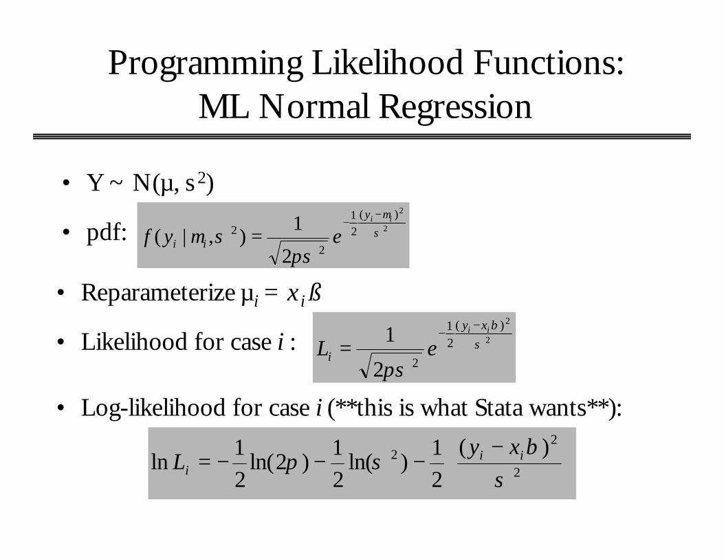
• Y ~ N(µ, s 2)
2
2)(21
2
2
2
1),|( σ
µ
πσσµ
iiy
ii eyf−
−=
2
2)(21
22
1 σβ
πσ
ii xy
i eL−
−=
−−−−= 2
22 )(
21
)ln(21
)2ln(21
lnσ
βσπ ii
i
xyL
• pdf:
• Reparameterize µi = xi ß
• Likelihood for case i :
• Log-likelihood for case i (**this is what Stata wants**):
Programming Likelihood Functions: ML Normal Regression
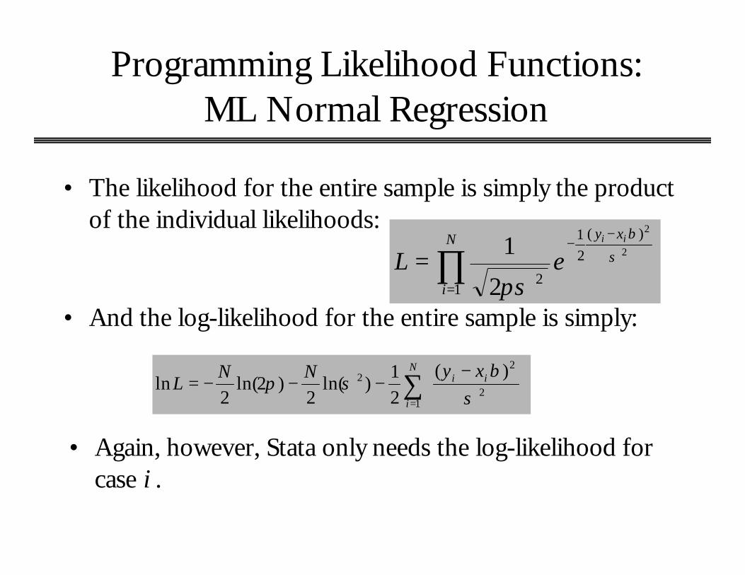
• The likelihood for the entire sample is simply the product of the individual likelihoods:
∏=
−−
=N
i
xy ii
eL1
)(21
2
2
2
2
1 σ
β
πσ
∑=
−−−−=
N
i
ii xyNNL
12
22 )(
21
)ln(2
)2ln(2
lnσ
βσπ
• And the log-likelihood for the entire sample is simply:
• Again, however, Stata only needs the log-likelihood for case i .

Programming Likelihood Functions: Syntax
• Goal: Write a program that Stata can use to maximize a log-likelihood function.
• First, Stata has 4 ML “evaluators”: lf, d0, d1, d2.• “lf” is the most basic evaluator; the “d” evaluators are for
more advanced programs. We’re only going to use “lf” in this session.

Programming Likelihood Functions: Syntax
program define prognameargs lnf theta1 theta2 ... tempvar tmp1 tmp2 ... quietly gen double `tmp1' = ... quietly replace `lnf' = ...
end
• `lnf’ is a variable to be filled in with values of the log-likelihood for case i (i.e., lnLi ).
• `theta1’ is associated with the first parameter, containing evaluation of the 1st equation: theta1i = x1i b
• `theta2’ is associated with the second parameter, containing evaluation of the 2nd equation: theta2i = x2i b

Programming Likelihood Functions: Syntax
• Global macros:$ML_y1 is a global macro for the name of the first dependent variable.$ML_y2 is a global macro for the name of the second dependent variable.

Onto the Machines: Start a .log File
Click here to start .log file.

Onto the Machines: Start a .log File
Change to .log
Programming Likelihood Functions: ML Normal Regression Program
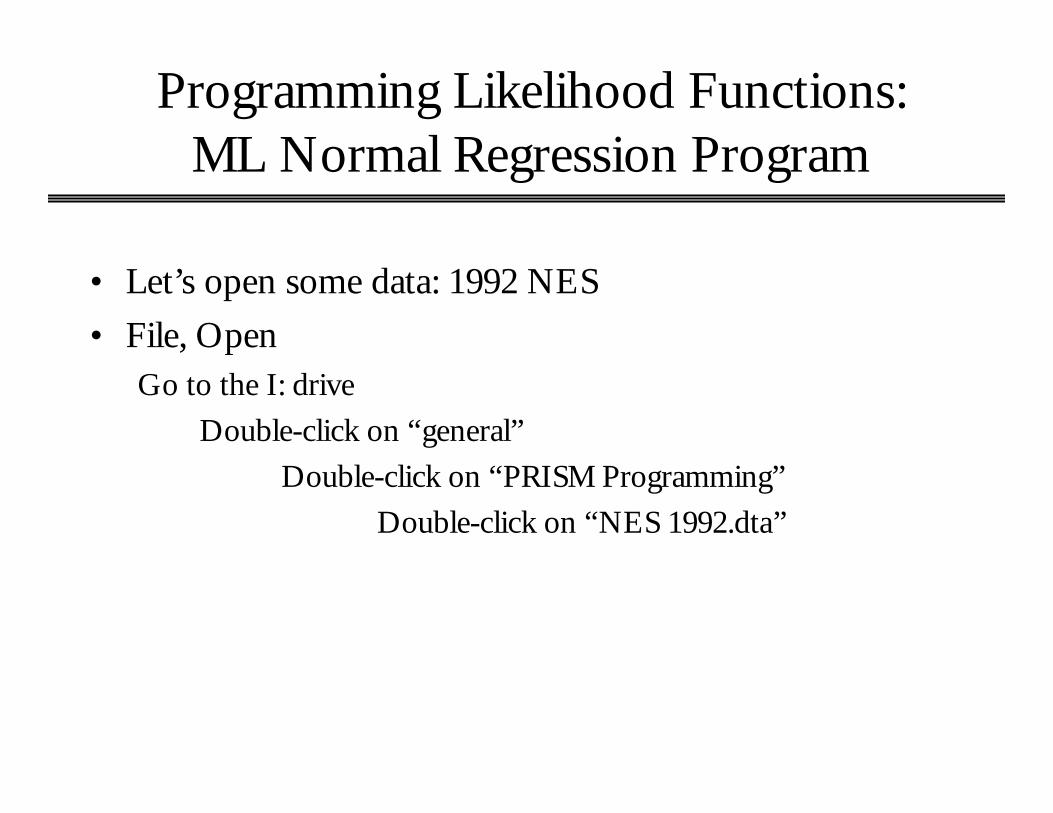
• Let’s open some data: 1992 NES• File, Open
Go to the I: driveDouble-click on “general”
Double-click on “PRISM Programming”Double-click on “NES 1992.dta”

Programming Likelihood Functions: ML Normal Regression Program
Click here to open new .do file.

Programming Likelihood Functions: ML Normal Regression Program
• Open “normreg” program from the .do file editor:Go to the I: drive
Double-click on “general”Double-click on “PRISM Programming”
Double-click on “normreg.do”

Programming Likelihood Functions: ML Normal Regression Program
−−−−= 2
22 )(
21
)ln(21
)2ln(21
lnσ
βσπ ii
i
xyL
Recall:
Run the program

Programming Likelihood Functions: Maximizing the Likelihood Function
• Once we’ve written the program, we need to tell Stata to estimate it. This takes two steps:
(1) ml model lf progname (eq1: y=x1 x2 x3)- or –
ml model lf progname (eq1: y=x1 x2 x3) (eq2: y=x1 x2 x3)- or –
ml model lf progname (eq1: y=x1 x2 x3) /parameter[If the second parameter is not reparameterized as a function ofcovariates, e.g., s2 in ML normal regression.]
(2) ml max

Programming Likelihood Functions: Maximizing the Likelihood Function
• Other useful commands to run after ml model:ml check verifies that the program you wrote worksml search searches for better starting valueslf0(#k LL0) reports a likelihood ratio test (included after the “ml
model” command), comparing fully specified model to an intercept only (i.e., null) model. The Wald test is produced by default. For the LR test, you need to specify the LL and the number of parameters for the intercept only model.

Programming Likelihood Functions: Estimating the ML Normal Model
• Let’s estimate a simple model; we’ll regress George H.W. Bush’s approval on PID and economic perceptions.

Programming Likelihood Functions: Estimating the ML Normal Model
Enter this; specifies model.
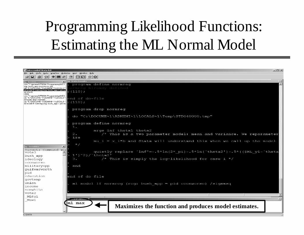
Programming Likelihood Functions: Estimating the ML Normal Model
Maximizes the function and produces model estimates.

Programming Likelihood Functions: Estimating the ML Normal Model

Programming Likelihood Functions: Comparing ML Reg to OLS
• OLS and ML Normal Regression produce identical parameter estimates. It can be shown that the analytical solution for ML Normal Regression is:
ß = (X’X)-1X’Ywhich is identical to the well-known formula for the OLS estimator.
• Standard errors will be different, though, because: – In ML:
– In OLS:
N
eN
ii∑
== 1
2
2σ
kN
eN
ii
−=
∑=1
2
2σ

Programming Likelihood Functions: Comparing ML Reg to OLS
Estimate this OLS.

Programming Likelihood Functions: Comparing ML Reg to OLS
Coefficients are identical, SEs are different.
s2 is slightly smaller for ML than OLS; that’s b/c denominator is N versus N-k.

Programming Likelihood Functions: Logit and Probit
• In binary response models, we want to model the probability of “success” for case i, i.e., Pr( yi=1) = ? i
• We parameterize ? i as a cumulative distribution function (cdf) of a particular distribution, i.e., F ( xi ß )– For logit, we use the logistic cdf:
)exp(1)exp(
)()1Pr(β
ββ
i
iii x
xxFy
+===
)()()1Pr( ββ iii xxFy Φ===– For probit, we use the normal cdf:
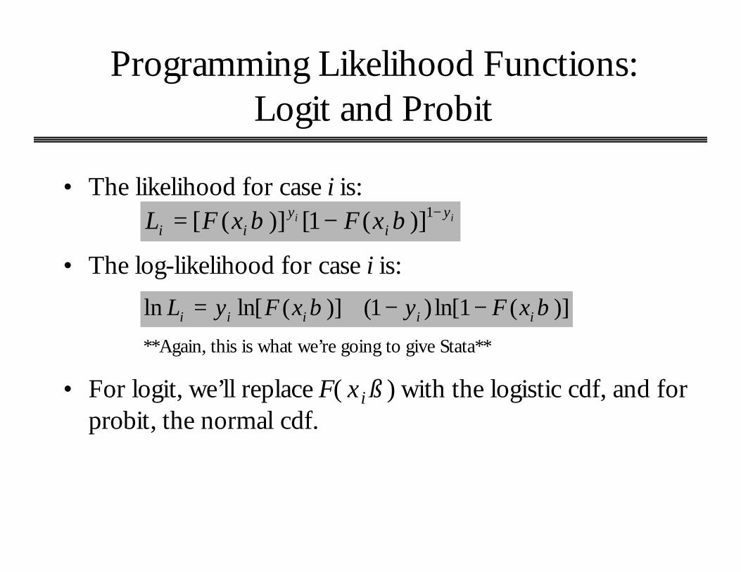
Programming Likelihood Functions:Logit and Probit
• The likelihood for case i is:ii y
iy
ii xFxFL −−= 1)](1[)]([ ββ
• The log-likelihood for case i is:
)](1ln[)1()](ln[ln ββ iiiii xFyxFyL −−+=
**Again, this is what we’re going to give Stata**
• For logit, we’ll replace F( xi ß ) with the logistic cdf, and for probit, the normal cdf.

Programming Likelihood Functions:Logit and Probit
• Open “mylogit.do” from the .do file editor.Go to the I: drive
Double-click on “general”Double-click on “PRISM Programming”
Double-click on “mylogit.do”

Programming Likelihood Functions:Logit and Probit
)](1ln[)1()](ln[ln ββ iiiii xFyxFyL −−+=Recall:
Run the program

Programming Likelihood Functions:Logit and Probit
Enter this. Simple vote choice model, 1=Bush, 0=otherwise
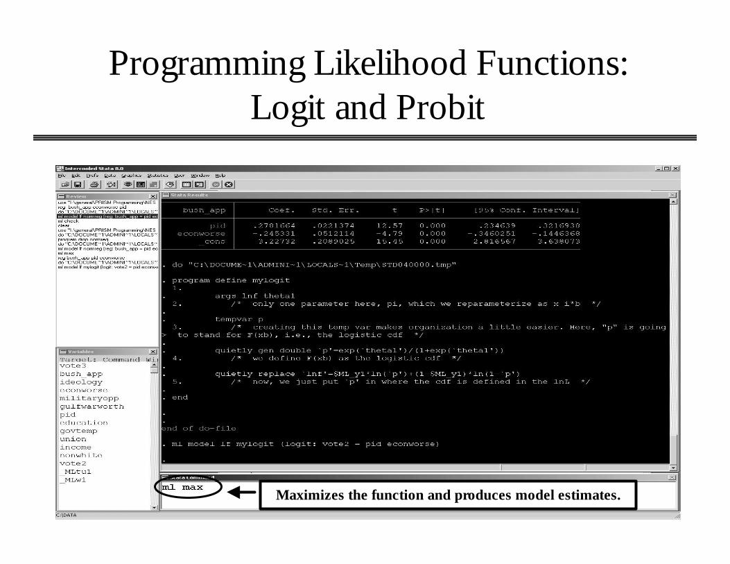
Programming Likelihood Functions:Logit and Probit
Maximizes the function and produces model estimates.

Programming Likelihood Functions:Logit and Probit

Programming Likelihood Functions:Logit and Probit
Identical to using canned logit command.

Programming Likelihood Functions: The Likelihood Ratio Test
• By default, “ml model” produces a Wald test for overall goodness of fit test (which tests that the coefficients are jointly equal to zero).
• To get an LR test, we need to: – Estimate an intercept only model to get LL0, the initial LL.– We need to specify k for the intercept-only model, which in this
case is 1.– After the “ml model” command, we enter lf0(k LL0).

Programming Likelihood Functions: The Likelihood Ratio Test
Estimates intercept only model

Programming Likelihood Functions: The Likelihood Ratio Test
Maximize the function.
This is LL0.

Programming Likelihood Functions: The Likelihood Ratio Test

Programming Likelihood Functions: The Likelihood Ratio Test
Maximize the function.

Programming Likelihood Functions: Probit Program

Programming Likelihood Functions: Heteroskedastic Regression
• Heteroskedastic regression allows us to model the factors that influence both the expected value of Y and the factors that affect the variability around that expected value (see Franklin 1991; Alvarez and Brehm 1995, 1997, 1998).
• In regression, we always assume homoskedasticity: s 2
• With het. reg., we’re explicitly interested in modeling the factors that influence .
• Good pedagogical example: it’s more complicated, it generates two sets of simultaneously generated coefficients. But, bottom line: all you have to do is know the likelihood function, and you can program it in Stata.
2iσ

Programming Likelihood Functions:Heteroskedastic Regression
• We parameterize as:
• Where the zi’s exogenous variables that influence the variability around the expected value, and gamma is a vector of parameters.
• Log-likelihood:
2iσ
γσ izi e=2
−−−−= γ
βγπ
izii
ii exy
zL2)(
21
21
)2ln(21
ln

Programming Likelihood Functions: Heteroskedastic Regression
−−−−= γ
βγπ
izii
ii exy
zL2)(
21
21
)2ln(21
ln

Programming Likelihood Functions: Heteroskedastic Regression

Programming Likelihood Functions: Heteroskedastic Regression

Programming Likelihood Functions: Split-Population Duration Model
• Standard duration models, which model the hazard of an event occurring, assume that all cases will eventually experience the event of interest.
• This assumption may not hold for the process under examination; if not, will produce incorrect inferences. – The timing of congressional overrides of Supreme Court
decisions (Hettinger and Zorn 2004).– Corporate and labor PAC contributions to congressional
candidates (Box-Steffensmeier et al. 2004).

Programming Likelihood Functions: Split-Population Duration Model
• The split population duration (SPD) model relaxes the assumption that all cases will eventually experience the event of interest (Schmidt and Witte 1988, 1989; Forster and A. Jones 2001; Box-Steffensmeier and B. Jones 2004).
• Simultaneously estimates two sets of coefficients:1. Explaining the likelihood of the event occurring (i.e., the
censoring indicator is the DV). 2. Explaining the timing of the event occurring, conditional on the
event having occurred in the first place.
Programming Likelihood Functions: Split-Population Duration Model
• LIMDEP is the only package that has a canned routine for the SPD. Great example of an advanced model that hasn’t made its way into a lot of stat packages. But you can program it yourself!
• Acknowledgements to Forster and Jones…

Programming Likelihood Functions: Split-Population Duration Model
)],(1ln[)1()],(ln[lnln θδδθδ iiiiiiii tGRtgRL +−−++=
survivor functionpdfcensoring indicator

Programming Likelihood Functions: Split-Population Duration Model
• Example: Explaining the incidence and timing of labor PAC contributions to incumbent House members, 1993-1994 (Box-Steffensmeier et al. 2004).
• We’re interested in the timing of contributions in an election cycle. Early money is “seed money” for a campaign effort, and it helps candidates raise more down the line (Jacobson 1992).
• We don’t expect labor PACs to contribute to every House incumbent, though. E.g., people trying to reform OSHA, or investigating the Teamsters.
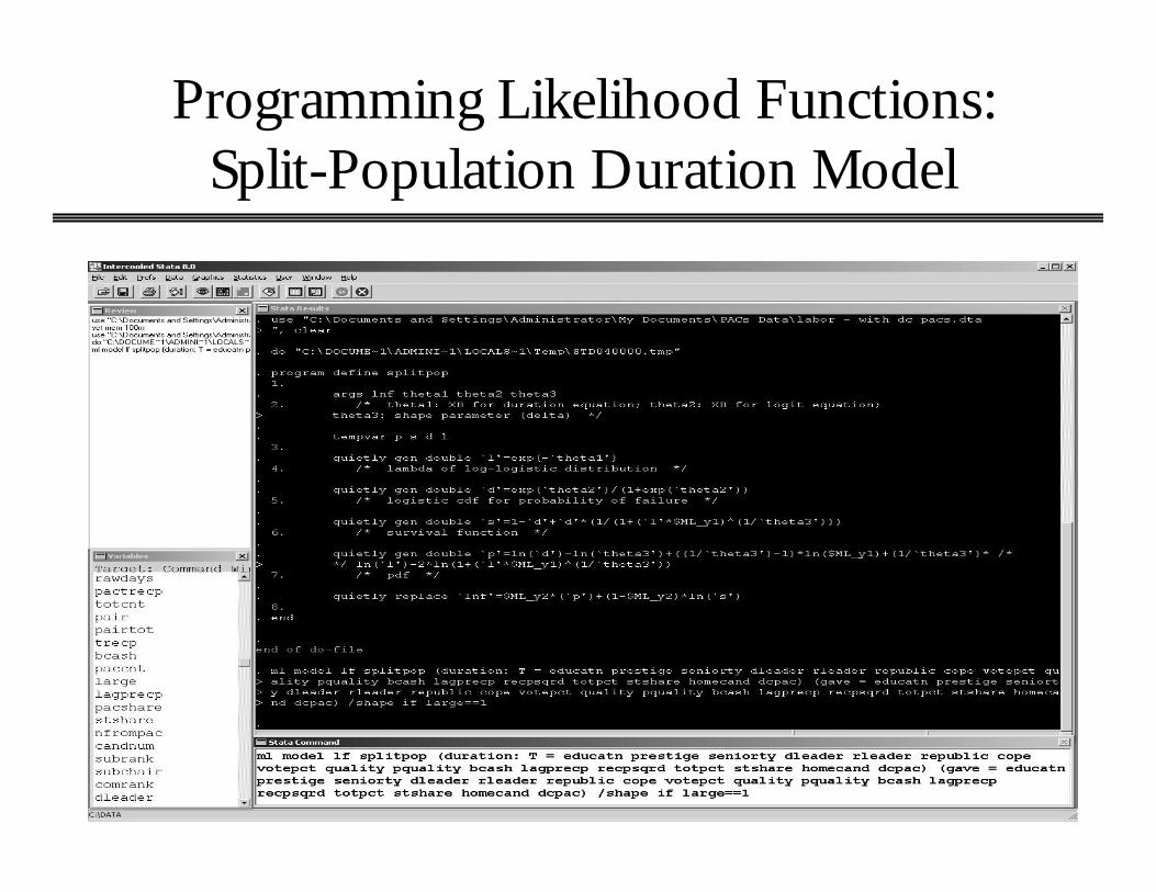
Programming Likelihood Functions: Split-Population Duration Model
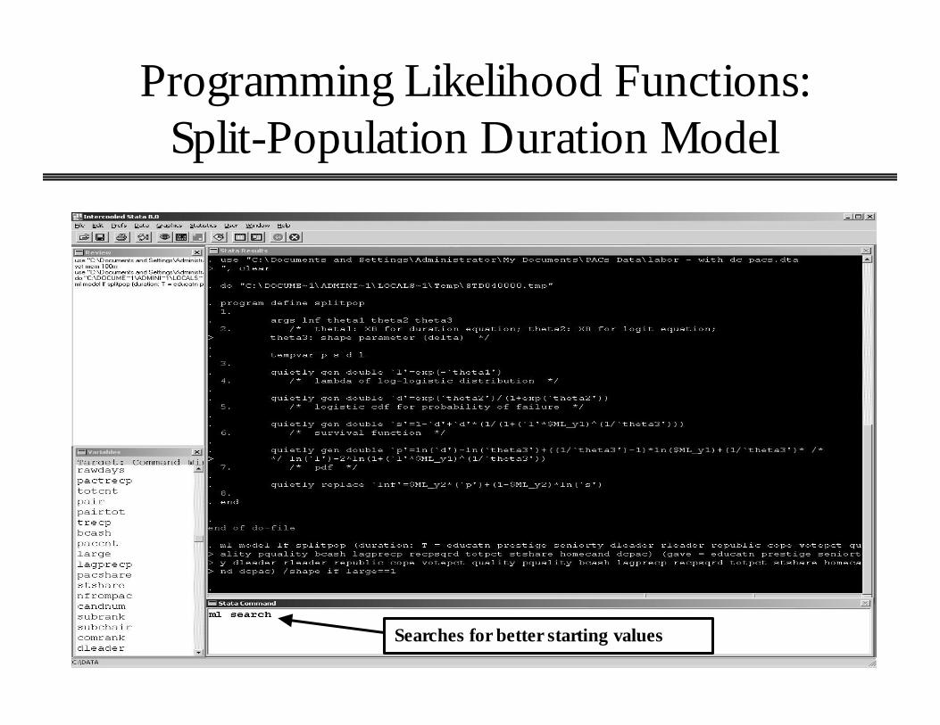
Programming Likelihood Functions: Split-Population Duration Model
Searches for better starting values

Programming Likelihood Functions: Split-Population Duration Model

Programming Likelihood Functions: Split-Population Duration Model
ml max
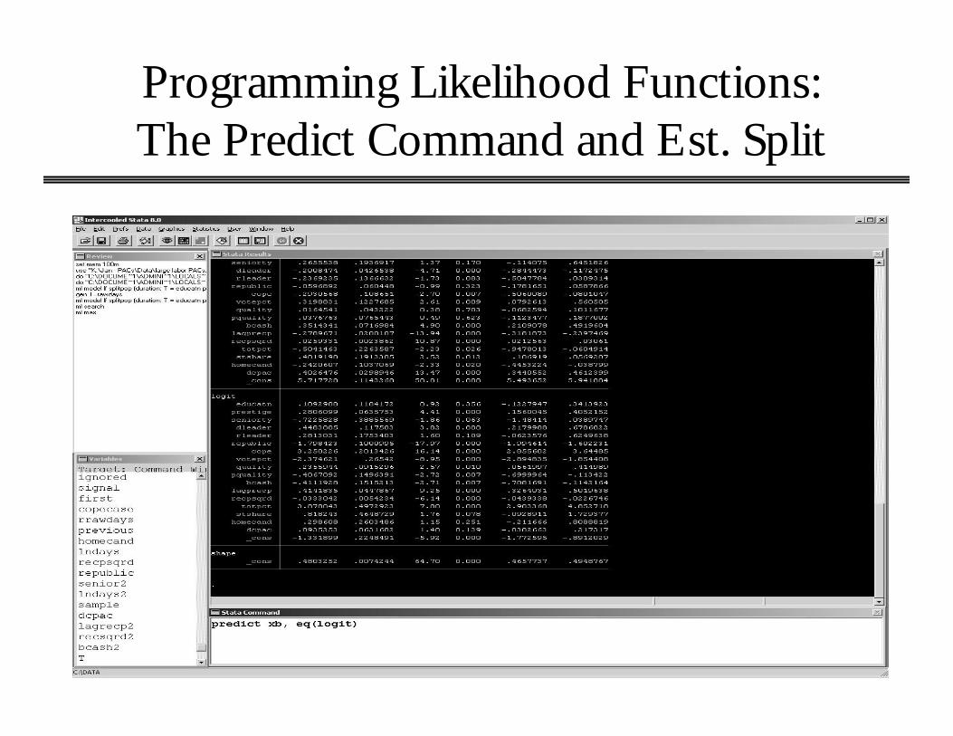
Programming Likelihood Functions: The Predict Command and Est. Split

Programming Likelihood Functions: The Predict Command and Est. Split
Calculates probability of the exchange of a contribution.

Programming Likelihood Functions: The Predict Command and Est. Split
Estimated split
Observed split

Programming Likelihood Functions: Conclusion
• Bottom line:– If you need to estimate a model that is not canned in a
popular software package, you can probably program it in Stata.
– All you need to know is the likelihood function!


