BREACH, REMEDIES AND DISPUTE SETTLEMENT IN TRADE AGREEMENTS
Giovanni MaggiRobert W. Staiger
Working Paper 15460http://www.nber.org/papers/w15460
NATIONAL BUREAU OF ECONOMIC RESEARCH1050 Massachusetts Avenue
Cambridge, MA 02138October 2009
We thank Kyle Bagwell, Chad Bown, Gene Grossman, Petros C. Mavroidis, TN Srinivasan, AlanSykes, participants in seminars at FGV- Rio, FGV-SP, PUC-Rio, Stanford and the World Trade Organization,and participants in the 2009 NBER Summer Institute and the conferences "The New Political Economyof Trade" at EUI (Florence), "The Economics, Law and Politics of the GATT-WTO" at Yale and "TheFestschrift in Honor of Alan V. Deardorff" at The University of Michigan for very helpful comments.The views expressed herein are those of the author(s) and do not necessarily reflect the views of theNational Bureau of Economic Research.
NBER working papers are circulated for discussion and comment purposes. They have not been peer-reviewed or been subject to the review by the NBER Board of Directors that accompanies officialNBER publications.
Breach, Remedies and Dispute Settlement in Trade AgreementsGiovanni Maggi and Robert W. StaigerNBER Working Paper No. 15460October 2009JEL No. D02,D86,F13,K12,K33
ABSTRACT
We provide a simple but novel model of trade agreements that highlights the role of transaction costs,renegotiation and dispute settlement. The model allows us to characterize the appropriate remedy forbreach and whether the agreement should be structured as a system of "property rights" or "liabilityrules." We then study how the optimal rules depend on the underlying economic and contracting environment.Our model also delivers predictions about the outcome of trade disputes, and in particular about thepropensity of countries to settle early versus "fighting it out."
Giovanni MaggiDepartment of EconomicsYale University37 Hillhouse Avenue Rm 27New Haven, CT 06511and [email protected]
Robert W. StaigerDepartment of EconomicsStanford UniversityLandau Economics Building579 Serra MallStanford, CA 94305-6072and [email protected]
1. Introduction
When governments make international commitments, what should be the legal remedy for
breach under their agreement? Should the entitlements assigned by the agreement take the
form of property rights,whereby an entitlement can only be removed from its holder through
a voluntary transaction, or of liability rules,whereby an entitlement can be removed from its
holder for the payment of legally determined damages? And what do these institutional rules
imply for the propensity of countries to settle early versus going to court?
In this paper we address these questions as they arise in the context of international trade
agreements. While our analysis applies to trade agreements generally, we pay particular at-
tention to the rules of the World Trade Organization (WTO) and the General Agreement on
Tari¤s and Trade (GATT), its predecessor. This is a natural institution on which to focus,
given its prominence in the world trading system.
Our analysis features the important possibility that governments may settle their di¤erences
without recourse to a ruling by the court, and hence bargain in the shadow of the law.1 Indeed,
Busch and Reinhardt (2006) report that two thirds of WTO disputes are resolved before a
nal ruling of the Dispute Settlement Body (DSB). Here the legal rules and remedies do not
directly determine the outcome, but they do impact the outcome indirectly by shaping what
governments can expect if their attempts at settlement fail. In this case the critical role played
by the DSB lies precisely in dening the disagreement point provided by the legal system. And
in the presence of transaction costs, these legal rules and remedies can have important e¢ ciency
consequences even when, as in the GATT/WTO, bargaining and settlement is the dominant
outcome.
These themes are virtually unexplored in the existing economics literature on trade agree-
ments, in part because the modeling of disputes in that literature does not accommodate the
possibility of settlement in a meaningful way and is therefore ill-equipped to provide a platform
for formal analysis of the questions raised above. By contrast, in the law and economics lit-
erature analogous questions and issues have been extensively studied in a domestic context as
they relate to the actions of private agents. There are two related literatures. A fundamental
question in the literature concerned with domestic contracts (see, for example, Schwartz, 1979,
1This phrase appeared in the title of a paper by Mnookin and Kornhauser (1979). Like us, those authorswere ...concerned primarily with the impact of the legal system on negotiations and bargaining that occuroutside the courtroom.(p. 950, emphasis in the original).
1
Ulen, 1984, and Shavell, 2006) is when contracting parties would want specic performance as
a remedy for contract breach and when they would instead prefer damage payments. There is
also a vast literature (the seminal contributions are Calabresi and Melamed, 1972, and Kaplow
and Shavell, 1996) that is concerned with the related question of when property rules are pre-
ferred to liability rules in the design of domestic law. A major goal of our paper is to initiate
the formal analysis of these themes in the context of international trade agreements.2
Looking across the GATT/WTO, one can see evidence of both liability rules and property
rules at work. For instance, there is broad agreement that in the early years GATT operated
in e¤ect as a system of liability rules, where breach remedies were similar to compensation for
escape clause actions and amounted to damage payments for the purpose of rebalancing(see
Jackson, 1969, p. 147, Schwartz and Sykes, 2002, and Lawrence, 2003, p. 29). However, it has
been observed that with the advent of the WTO the remedy for breach has moved away from
a system of damage payments and toward specic performance or compliance(see Jackson,
1997, Charnovitz, 2003, and Pelc, 2009), resulting in an institution where some entitlements
(e.g. the prohibitions against quantitative restrictions, export and to some extent domestic
subsidies, and discriminatory trade tari¤s) are now generally protected by property rules while
others (e.g., negotiated tari¤ bindings) are still protected by liability rules through applicable
escape clauses (and Pelc, 2009, argues that these escape clauses are themselves evolving toward
property rules as well). This interpretation of the evolution of the GATT/WTO is itself a
matter of debate among legal scholars (see Hippler Bello, 1996 and Schwartz and Sykes, 2002
who argue that the WTO can still best be viewed as a system of liability rules), but it is
clear that the choices that determine whether the GATT/WTO behaves more like a system of
property rules or rather liability rules are a key feature of institutional design. Our paper aims
at contributing toward an understanding of the forces that explain these choices.
In the domestic context that is the focus of the law and economics literatures, transac-
tion costs are typically associated with private information or other bargaining frictions. Such
frictions are surely present as well in international bargaining, but in the international con-
text there is an additional feature that is particularly salient: there generally does not exist
an e¢ cient government-to-government transfer mechanism that can be used to make damage
payments, either to settle disputes or to compensate for the exercise of escape clauses. In the
2Lawrence (2003) provides a lucid treatment of these themes as they relate to international trade agreementsat an informal level, and Srinivasan (2007) contains a related discussion.
2
GATT/WTO, the typical means by which one government achieves compensation for the harm
caused by another governments actions is through counter-retaliation,that is, by raising its
own tari¤s above previously negotiated levels. Such compensation mechanisms entail impor-
tant ine¢ ciencies (deadweight loss) that, while plausibly absent in the domestic private agent
context, introduce a novel transaction cost in the international context.
A major point of departure of our model is precisely this di¤erence between the domestic
private agent setting and the international government-to-government setting. In particular, we
consider a setting where governments, operating in the presence of ex-ante uncertainty about
the joint benets of free trade (which could be positive or negative due to the possible presence
of political economy factors), contract over trade policy and dene a mandate for the DSB in
the event that contract disputes should arise ex post, once uncertainty has been resolved and
trade policies are chosen. We assume that transfers between governments are costly and that
the marginal cost of transfers is (weakly) increasing in the magnitude of the transfer.
We consider agreements that specify a baseline commitment to free trade but allow the
importing government to escape (breach) this commitment by compensating the exporter with
a certain amount of damages. If the level of damages is set either at zero or at a level so high
that the importing government would never choose to breach, then this amounts to a property
rule in which either the entitlement to protect is assigned to the importing government or the
entitlement to free trade is assigned to the exporting government. If instead damages are set at
an intermediate level, then this is a liability rule. Our formalization of damages for breach can
be interpreted in either of two ways. The rst is that breach damages are specied explicitly
in the contract in the form of an escape clause; the second is that the contract species a
rigid free trade commitment, but the DSB may be given a mandate to require the payment of
damages in case of breach. As we have indicated above and discuss further below, both of these
interpretations are relevant for the GATT/WTO.
We assume that the DSB, if invoked, initiates an investigation and observes a noisy signal of
the joint benets of free trade, and issues a ruling based on this imperfect information. At the
time when the DSB can be invoked, the governments are uncertain about the outcome of the
DSB investigation and hence about the DSB ruling, and subject to this uncertainty must decide
whether to invoke the DSB or to settle. And if a DSB ruling is reached, the governments can
renegotiate the ruling; this is a further possibility for renegotiation and settlement, in addition
to the possibility before any DSB ruling which we already mentioned.
3
These two features of our model the possibility that governments negotiate an early
settlement under uncertainty about the DSB ruling, and the possibility of a later settlement
in which the DSB ruling is renegotiated constitute a second important point of departure
from the law-and-economics literature discussed above. Allowing governments to be uncertain
about the DSB ruling is important because, as will become clear, this allows for the possibility
that the governments may not settle early; and as a consequence, the model generates a variety
of predictions regarding when governments settle early or a dispute arises in equilibrium, and
how the disputes are resolved. And allowing for the possibility of later settlement generates
predictions about the circumstances under which a DSB ruling is renegotiated in equilibrium.3
We start with a benchmark scenario in which the DSB receives no information ex post, and
we consider the impact of ex-ante uncertainty over the joint benets of free trade. We nd
that a property rule, which either demands strict performance or permits complete discretion
in the choice of trade policy, is optimal if ex-ante uncertainty is su¢ ciently low, whereas a
liability rule tends to be optimal when ex-ante uncertainty is high. This nding suggests that,
as uncertainty over the joint benets of free trade falls, the optimal institutional arrangement
should tend to move away from liability rules toward property rules; and that liability rules
should be more prevalent than property rules in issue areas characterized by a higher degree of
uncertainty over the joint benets of free trade, and vice-versa.
Next we turn to the more general case in which the DSB observes a noisy signal ex post
about the joint benets of free trade. In this case, if ex-ante uncertainty about the joint benets
of free trade is small, a property rule is again optimal, but with the assignment of entitlements
contingent on the signal received by the DSB; and if ex-ante uncertainty is su¢ ciently large,
a liability rule again tends to be optimal, but with the DSB reducing the level of damages
when it receives a signal that the joint benets from free trade are smaller or negative. We also
establish that, for a given degree of ex-ante uncertainty, if the noise in the DSB signal is itself
su¢ ciently small, a property rule is optimal, with the assignment of entitlements contingent on
the signal. This nding suggests that, as the accuracy of DSB rulings increases, the optimal
institutional arrangement should tend to move away from liability rules toward property rules.
More broadly, if one accepts that the accuracy of DSB rulings has increased over time, or
that the degree of ex-ante uncertainty about the joint benets of free trade has fallen over time,
3As we discuss later in the paper, subsequent to DSB rulings it is not uncommon for WTO disputes ultimatelyto be settled through mutually agreed solutionsbetween the disputing parties rather than implementation ofthe ruling, corresponding roughly to a renegotiation of the DSB ruling in our formal analysis.
4
then our model predicts a gradual shift from liability rules to property rules. As we indicated
above, a number of legal scholars maintain that this shift can be seen in the GATT/WTO.
We also nd that, in the circumstances where a liability rule is optimal, it is never optimal to
set damages high enough to make the exporter whole.This runs counter to the presumption
established by the e¢ cient breachperspective of the law-and-economics literature, according
to which damages should be set at a level that makes the injured party whole so that breach
occurs whenever it is optimal to buy out the injured party. In fact, this presumption is
often extended informally to the context of the WTO, where it is sometimes suggested that
the principle of reciprocity which guides much of the GATT/WTO remedy system falls short
because it does not make the injured party whole (see, for example, Charnovitz, 2002, and
Lawrence, 2003). Our nding points out an important caveat in this reasoning: simply put, in
the WTO context, the damages paid for breach often take the form of counter-retaliation on
the part of the injured party, and this is an ine¢ cient means of compensation that, from an
ex-ante perspective, should not be permitted to an extent that makes the injured party whole.
In addition, we nd that the damages for breach should be responsive to both the harm
caused to the exporter and the benet garnered by the importer. We relate this nding to the
WTO Agreement on Safeguards, and suggest that it may be helpful in interpreting the WTO
rules on compensation for escape clause actions.
Our model generates interesting insights also with regard to the role of transaction costs in
determining the optimal rules. We nd that a property rule tends to be preferable to a liability
rule when the cost of transfers is high. We also examine the impact of frictions in ex-post
bargaining, by comparing the case of frictionless ex-post bargaining with the extreme opposite
case in which ex-post bargaining is not feasible, and nd that the introduction of frictions in
bargaining may favor property rules over liability rules. These results contrast with the ndings
in the law-and-economics literature that liability rules tend to be preferable to property rules
when transaction costs are high (Calabresi and Melamed, 1972, and Kaplow and Shavell, 1996).
Next we consider when disputes arise in equilibrium and how disputes are resolved. We nd
that early settlement of disputes is more likely when, at the time of contracting, there is more
uncertainty about the future joint benets from free trade; and we nd that early settlement
occurs when the joint benets of free trade turn out to be either very high or very low. We
also nd that, conditional on the DSB being invoked, the ruling is implemented when the DSB
receives information that the joint benets of free trade are either very high or very low, and
5
consequently sets a very high/low level of damages; but the DSB ruling is renegotiated if the
realized signal, and hence the level of damages set by the DSB, lies in an intermediate range.
A corollary is that renegotiation of DSB rulings need not reect a bad(inaccurate) ruling.
Finally, we consider the possibility that the cost of granting transfers di¤ers across the two
countries, and we interpret the high-cost country as a developing country. We nd that there
is a tendency for developed countries to impose more protection as a result of early settlements
than developing countries. In addition we nd that there is a pro-trade (anti-trade) selection
bias in DSB rulings when a developed country (developing country) is the respondent.
Beyond the literature we have already mentioned, there are a number of additional papers
that are related to ours. Like us, Beshkar (2008a,b) considers the possibility of e¢ cient breach
with non-veriable political pressures and costly transfers, but his model di¤ers from ours in a
number of important ways: most signicantly, he does not allow for the possibility of renegoti-
ation and settlement, which as we have emphasized is central to our analysis. Similarly, Howse
and Staiger (2005) investigate whether the GATT/WTO reciprocity rule might be interpreted
as facilitating e¢ cient breach, but they do not consider the possibility of settlement either.
Our paper is also related to Maggi and Staiger (2008). But that paper abstracts from issues of
costly transfers and settlement to highlight instead contract vagueness and interpretation.4
The rest of the paper proceeds as follows. The next section lays out the basic model.
Section 3 examines the nature of the optimal rules. Section 4 focuses on the outcome of
disputes. Section 5 considers two extensions: a more general informational environment where
uncertainty can be multi-dimensional, and a more general class of contracts that allows not
only for a stickassociated with protection, but also for a carrotassociated with free trade.
Section 6 concludes. All proofs are contained in the Appendix.
2. The Basic Model
We focus on a single industry in which the Home country is the importer and the Foreign
country is the exporter. The government of the importing country chooses a binary level of
4Bagwell and Staiger (2005), Martin and Vergote (2008) and Bagwell (2009) consider models with privatelyobserved political pressures, but they do not consider the role of a court (DSB) and focus instead on self-enforcement issues (from which we abstract). Park (2009) does consider the role of the DSB in a setting withprivately observed political pressures, but the DSB is formalized as a device that automatically turns privatesignals into public signals, without any ling decisions by governments, and hence his model cannot make adistinction between renegotiation/settlement and the triggering of DSB rulings. See also Ethier (2001) for anearly attempt to formalize the role of the DSB and its impact on the resolution of disputes.
6
trade policy intervention for the industry, which we denote by T 2 fFT; Pg: Free TradeorProtection.5 We assume that the exporting government is passive in this industry.
At the time that the Home government makes its trade policy choice, a transfer may also
be exchanged between the governments, but at a cost. Here we seek to capture the feature
that cash transfers between governments are seldom used as a means of settling trade disputes,
while indirect (non-cash) transfers, such as tari¤ adjustments in other sectors or even non-trade
policy adjustments, are more easily available.6 To allow for this possibility in a tractable way,
we let b denote a (positive or negative) transfer from Home to Foreign, and we let c(b) denote
the deadweight loss associated with the transfer level b. We assume that c(b) is non-negative,
(weakly) convex and smooth everywhere, with the natural features that c(0) = 0 and c(b) > 0
for b 6= 0. Finally, it is convenient to assume that the deadweight loss c(b) is borne by the
country that makes the transfer: thus, the loss is borne by Home (Foreign) if b > 0 (b < 0).
The importing governments payo¤ is given by
!(T; b) = v(T ) b c(b)I; (2.1)
where v(T ) is the importing governments valuation of the domestic surplus associated with
policy T in the sector under consideration, and I is an indicator function that is equal to one
if Home makes the transfer (i.e., if b > 0) and equal to zero otherwise. We have in mind that
v(T ) corresponds to a weighted sum of producer surplus, consumer surplus and revenue from
trade policy intervention, with the weights possibly reecting political economy concerns (as
in, e.g., Baldwin, 1987, and Grossman and Helpman, 1994). As we noted above, the exporting
government is passive in this industry; its payo¤ is therefore
!(T; b) = v(T ) + b c(b)I; (2.2)
where v(T ) is the exporting governments valuation of the foreign surplus associated with
policy T , and I is an indicator function that is equal to one if Foreign makes the transfer (i.e.,
if b < 0) and equal to zero otherwise.
5Our assumption of a binary policy instrument helps to keep our analysis tractable, and captures reasonablywell a variety of non-tari¤ policy choices, such as regulatory regimes or product standards, that are discrete innature. Many of the trade disputes in the GATT/WTO focus on these kinds of policy issues.
6The resolution of GATT/WTO disputes has, with one exception, never involved cash transfers (the oneexception to date is the US-Copyright case; see WTO, 2007, pp. 283-286). However, in the context of a tradedispute countries do sometimes achieve the indirect payment of compensation through the WTO self-helpmethod of counter-retaliation in other sectors. And WTO disputes that are settled by a mutually agreedsolutionunder Article 3.6 of the WTO Dispute Settlement Understanding (either before or after a DSB ruling)may involve a variety of indirect transfer mechanisms.
7
Using (2.1) and (2.2), the joint payo¤ of the two governments is denoted as and given by
(T; b) = v(T ) + v(T ) c(b): (2.3)
We assume that Home always gains from protection, and we denote this gain as
v(P ) v(FT ) > 0:
This gain may be interpreted as arising from some combination of terms-of-trade and political
considerations. On the other hand, we assume that Foreign always loses from protection, and
we denote this loss as
v(FT ) v(P ) > 0:
The joint (positive or negative) gain from protection is then .In this simple economic environment, the rst best(joint-surplus maximizing) outcome
is easily described: if > 0 (or > ), the rst best is T = P and b = 0, and if < 0 (or
< ), the rst best is T = FT and b = 0. Notice that b always equals zero under the rst
best, because transfers are costly to execute. For future use, we denote by FB the rst-best
joint payo¤ level.
We assume that governments are ex-ante uncertain about , but they observe ex post. If
were veriable (i.e. observed ex post by the court/DSB), of course the governments could write
a complete contingent contract, and the problem would be uninteresting. We are interested
instead in an imperfect-contracting scenario, where such a complete contingent contract cannot
be written. We consider the simplest scenario of this kind that allows us to make the relevant
points. We assume that is ex-ante known to all, so that all the uncertainty in originates
from , and that is not veriable. In section 5 we extend our results to the case in which
is also uncertain (and not veriable). There is also a further motivation besides simplicity
for considering the case in which is known ex ante. This is the case that is most favorable to
the standard argument for a liability rule, according to which e¢ ciency can be induced if the
exporter is made whole with a damage payment of in the event of breach. We will show that,
even in this most-favorable case, the standard argument for a liability rule must be qualied in
our setting along a number of important dimensions.
We denote by h( ) the ex-ante distribution of , which we assume to be common knowledge
(to the governments as well as the DSB). Unless otherwise noted, we assume that the support
of is bounded. Finally, to make things interesting, we assume that the value = is in the
8
interior of the support of , so that the rst-best is P in some states (when > , and hence
> 0) and FT in some states (when < , and hence < 0).
The fact that governments cannot write a complete contingent contract does not neces-
sarily imply ine¢ ciencies. If international transfers were costless (no deadweight loss), then
governments could always achieve the rst-best by engaging in ex-post (i.e., after observing
) negotiations over policies and (costless) transfers.7 If international transfers are costly, on
the other hand, the rst best cannot be achieved in general, but ex-ante joint surplus may be
enhanced by writing a contract ex ante (before is realized), and dening a role for the DSB
in the event that contract disputes arise ex post. We look for the contract/DSB combination
that maximizes ex-ante joint surplus.8
We may now describe the timing of events. The game is as follows:
stage 0. Governments write the contract and dene the role of the DSB.
stage 1. The state of the world is realized and observed by the governments.
stage 2. The importer proposes a T and a b that can di¤er from the terms of the contract. The
exporter either accepts the proposal or les with the DSB.
stage 3. If invoked, the DSB issues a ruling.
stage 4. The importer can propose a deviation from the ruling. The exporter either accepts the
proposal (so that the DSB ruling is not enforced) or demands enforcement of the ruling.
stage 5. Trades occur and payo¤s are realized.
Note that we allow ex-post renegotiation of the initial contract (in stage 2) as well as
renegotiation of the DSB ruling (in stage 4); and we assume that the importer makes take-or-
leave o¤ers. Opportunities for renegotiation are central to our analysis, and as we indicated
7We abstract from issues of enforcement here and simply assume that bargaining outcomes between the twogovernments are enforced.
8There are three ways to justify this emphasis on the maximization of the governmentsex-ante joint surplus.One possibility is to allow for costless ex-ante transfers, i.e., transfers at the time the institution is created. Thisjustication is not in contradiction with our assumption of costly ex-post transfers, if it is interpreted as reectingthe notion that the cost of transfers can be substantially eliminated in an ex-ante setting such as a GATT/WTOnegotiating round where many issues are on the table at once (see, for example, the discussion in Hoekmanand Kostecki, 1995, Ch. 3). A second possibility would be to keep the single-sector model and introduce a veilof ignorance, so that ex-ante there is uncertainty over which of the two governments will be the importer andwhich the exporter. And a third possibility would be to introduce a second mirror-image sector.
9
in the Introduction and describe further below, they are an important feature of the dispute
resolution process for trade agreements such as the GATT/WTO. By contrast, the assumption
of take-or-leave o¤ers makes our analysis easier, but it is not critical for our results.
2.1. The feasible contracts and the role of the DSB
We next describe the feasible contracts and the role of the DSB. We consider a family of menu
contracts that allow the importer to choose between (i) setting FT and (ii) setting P and
compensating the exporter with a payment bD. Or, using slightly di¤erent terminology, these
contracts specify a baseline commitment (FT ) but allow the importer to escape/breach this
commitment by paying a certain amount of damages.
Note that this family of contracts includes two contracts of particular interest: (i) a rigid
fFTg contract, which corresponds to the case in which bD is set at a prohibitively high (orinnite) level; we often refer to this contract as one that requires strict performance under
all circumstances, or in short, a performance contract,and (ii) discretion over trade policy,
which corresponds to the case in which bD = 0. Thus, as the level of damages bD goes from zero
to prohibitive, the menu contract spans all the interesting possibilities, ranging from discretion
to a contract that stipulates (non-prohibitive) damages to a strict performance contract.
Observe as well that setting damages at either zero or a prohibitive level amounts to es-
tablishing a property rule, in which as a legal matter the right to protect is granted to the
importer (when damages are set to zero) or the right to free trade is granted to the exporter
(when damages are set at a prohibitive level). And setting damages strictly between zero and
the prohibitive level amounts to establishing a liability rule. In what follows we also draw links
between our results and the law-and-economics literature that is concerned with the choice
between property rules and liability rules.
We initially consider a benchmark scenario in which the DSB does not receive any informa-
tion ex post (section 3.1), so that the governments have no uncertainty about the DSB ruling
at the ex-post negotiation stage, and later (section 3.2) we consider the case in which the DSB
can observe a noisy signal of (which we denote ), so that governments are uncertain about
the DSB ruling at the ex-post negotiation stage. In this latter case, we consider a wider class
of contracts, where bD can be contingent on : given the bD schedule specied by the contract,
if the DSB is invoked, it estimates the damages due to the exporter based on its information.
There are two interpretations of the optimization problem we have just outlined. The rst,
10
more direct interpretation is that governments design a contract that species a baseline com-
mitment to free trade but includes an explicit escape clause. Some WTO contracts/clauses take
this form, for example negotiated tari¤ commitments and the associated GATT Article XIX
Escape Clause and/or Article XXVIII renegotiation provisions.9 Given this interpretation, we
may ask what is the appropriate level of damages that should be included in the contract: the
answer here is relevant for the design of explicit escape clause provisions. Under this inter-
pretation a DSB ruling simply enforces contract performance (i.e. ensures that the importing
government either selects FT or pays the contractually specied damages).
A second interpretation is that governments design an institution consisting of two parts: (i)
a rigid fFTg contract with no contractually specied means of escape; and (ii) a mandate for theDSB, which instructs the DSB to enforce a certain remedy (the payment bD) that the importing
government must pay the exporting government in case of breach. If the breach remedy is
prohibitive in all states of the world, we say that the DSB is instructed to enforce contract
performance. At the opposite extreme, if bD = 0, so that the DSB permits breach at zero cost,
the outcome is the same as with full discretion, just as under the previous interpretation. In
the WTO, many contractual commitments are best described as rigid (e.g., the ban on export
subsidies). And we may then ask what is the appropriate remedy for breach that should be
made available by the DSB: the answer is relevant for the mandate/design of the DSB.10
Our analysis applies equally well under either of these interpretations, i.e., whether the
breach remedy is specied in the contract or rather in the DSB mandate. (In a richer model,
both could coexist, with general breach possibilities determined by the mandate of the DSB
and more specic breach possibilities made available in the contract). In either case, the level
of the breach remedy is important for the same reason: it serves to dene the disagreement
point provided by the legal system should ex-post negotiations between the governments fail.
9The non-violation nullication-or-impairment clause of the GATT can also be interpreted along the lines ofan escape clause, as it permits countries to in e¤ect breach their negotiated market access commitments withunanticipated changes in domestic policies and pay damages to injured parties as a remedy.10In reality, the role of DSB investigations in a setting such as the GATT/WTO is typically twofold: rst, to
establish whether or not breach exists; and second, to determine damages if this becomes necessary as part ofa remedy. In the model we develop here, the rst role is trivially fullled, because we have assumed that thecontractually obligated policy is clearly specied and the policy choice is publicly observable. This assumptionallows us to concentrate on the second DSB role listed above (i.e., the determination of damages), which is thefocus of our analysis. Of course, a typical GATT/WTO dispute involves multiple claims of breach which theDSB must evaluate, and so in practice the breach determination itself helps to determine the level of damages,and the two roles of the DSB are intertwined.
11
2.2. The ex-post Pareto frontier
We complete our description of the basic model by describing the ex-post Pareto frontier and
how it varies with the realized state ( ). The ex-post frontier plays a key role in the analysis,
since it describes the set of feasible payo¤s for the negotiations in both stages 2 and 4.
To describe the ex-post frontier, we partition the possible realizations of into four intervals
(or regions): Region I ( << 0), where the e¢ ciency gains from FT are large; Region II
( < 0), where the e¢ ciency gains from FT are relatively small; Region III ( > 0), where the
e¢ ciency gains from P are relatively small; and Region IV ( >> 0), where the e¢ ciency gains
from P are large. Figure 1 depicts the ex-post Pareto frontier for a representative realization
in each of Regions I through IV. For each region, the Pareto frontier corresponds to the outer
envelope of two concave sub-frontiers, one passing through point P (and associated with T = P
and various levels of the transfer b), the other passing through point FT (and associated with
T = FT and various levels of b): the concavity of each sub-frontier reects the convexity of
c(b). Recalling our assumption that the value = is in the interior of the support of , it
follows that Regions II and III are non-empty. By contrast, Regions I and/or IV are relevant
only if the support of is su¢ ciently large.
The top left panel of Figure 1 depicts the ex-post frontier for Region I. Here, the e¢ ciency
gains from FT are large, and as a consequence, achieving the frontier always requires T =
FT ; moreover, the frontier is concave (in the relevant part of the payo¤ space), reecting the
mounting ine¢ ciency associated with greater transfers as we move away (in either direction)
from point FT (where ! = !(FT; 0) and ! = !(FT; 0)). The bottom right panel of Figure
1 depicts the ex-post frontier for Region IV. Here the e¢ ciency gains from P are large, and so
achieving the frontier always requires T = P ; and again, in Region IV the frontier is concave,
reecting the mounting ine¢ ciency associated with greater transfers as we move away from
point P (where ! = !(P; 0) and ! = !(P; 0)).
Now consider the top right panel of Figure 1, which depicts the ex-post frontier for Region
II. Here, FT entails a higher joint payo¤ than P , but by a relatively small amount, and as
a consequence neither of the policies FT or P Pareto-dominates the other; and the frontier
is piece-wise concave but globally non-concave, because both the policy T and the transfer b
change as we move along the frontier. The lower left panel of Figure 1 depicts the ex-post
frontier for Region III. Here the situation is qualitatively similar to Region II, except that now
it is P that entails a higher joint payo¤ (by a relatively small amount).
12
As we have noted, Regions I and IV are relevant only if the support of is su¢ ciently large,
and as should now be apparent, the bargaining environment in Regions I and IV is very di¤erent
from that in Regions II and III; as a consequence, the degree of uncertainty over turns out
to be a key determinant of the optimal breach remedy. Also, as can be seen by inspection of
Figure 1, making the support of larger has qualitatively similar e¤ects as making the cost of
transfers smaller (holding everything else constant); hence, the cost of transfers is also pivotal
in determining the optimal breach remedy.
For now it su¢ ces to observe that, for any realized , the outcome of the negotiations is
determined by the features of the relevant ex-post frontier and the position of the disagreement
point relative to the frontier. And as we have observed, the disagreement point is shaped by
the level of damages bD.
3. The Optimal Rules
We now turn to a complete analysis of the game. We begin with the benchmark scenario in
which the DSB receives no information ex post, so that governments have no uncertainty about
the DSB ruling at the stage of ex-post negotiations. We then consider noisy DSB investigations.
3.1. A benchmark scenario: the DSB receives no information ex post
In this section we suppose that the DSB receives no information ex post, and thus bD must be
noncontingent. For a given bD, we solve the game by backward induction, and then determine
the value of bD that maximizes ex-ante joint surplus.
The backward induction analysis is simplied by observing that, in this benchmark scenario,
the outcome of the stage-4 bargain must be the same as the outcome of the stage-2 bargain.
Intuitively, since bargaining is e¢ cient, the outcome of the stage-4 subgame is on the Pareto
frontier for any state call this point Q4. Now consider what happens at stage 2 when
governments negotiate after observing the state. At this stage governments anticipate perfectly
the DSB decision, and so the threat point of this negotiation is simply point Q4. Since Q4 is
on the Pareto frontier, there is no possible Pareto improvement that governments can achieve
at stage 2 over the threat point, and hence the equilibrium outcome of the stage-2 bargain is
the same as that of the stage-4 bargain. (For this reason, in this section we often refer to the
bargain without specifying the stage in which the bargain occurs.)
13
In light of this observation, to determine the optimal bD we just need to derive the equilib-
rium joint surplus of the stage-4 bargain as a function of bD, take the expectation of this joint
surplus over all states , and optimize bD. Here we sketch the intuition behind our results,
relegating proofs to the Appendix.
Given that FT is the rst-best policy in Regions I and II while P is the rst-best policy in
Regions III and IV, it might be expected that e¢ ciency considerations would push toward a high
value of bD when the state falls in Regions I or II, and toward a low value of bD when it falls in
Regions III or IV. And given this expectation, it seems natural that the optimal level of bD would
then be somewhere in the middle (i.e., a liability rule), since there is uncertainty over whether
the realized state lies in Regions I/II or Regions III/IV. But things are more complicated, in
part because as we have noted the ex-post frontier can be non-concave (Regions II and III), and
in part because the importer has two distinct choices under disagreement (FT with no transfer
or P with transfer bD), only one of which is activeunder the circumstances (i.e., the choice
preferred by the importer given the realized ).
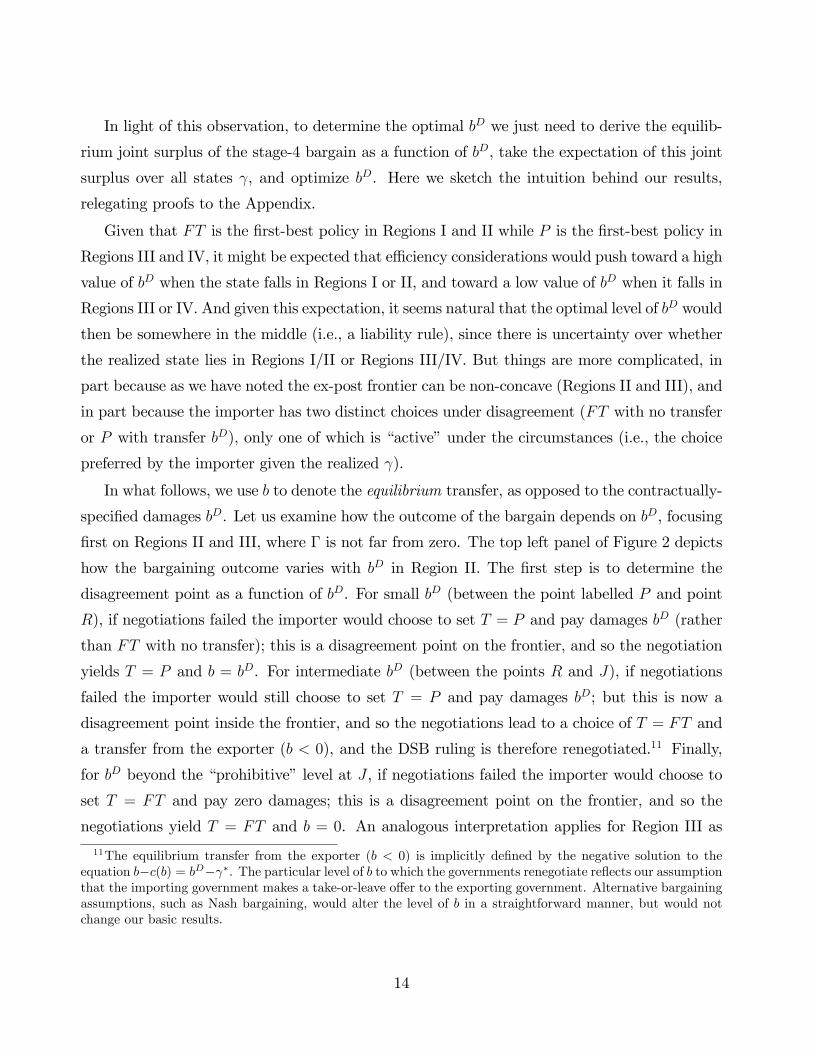
In what follows, we use b to denote the equilibrium transfer, as opposed to the contractually-
specied damages bD. Let us examine how the outcome of the bargain depends on bD, focusing
rst on Regions II and III, where is not far from zero. The top left panel of Figure 2 depicts
how the bargaining outcome varies with bD in Region II. The rst step is to determine the
disagreement point as a function of bD. For small bD (between the point labelled P and point
R), if negotiations failed the importer would choose to set T = P and pay damages bD (rather
than FT with no transfer); this is a disagreement point on the frontier, and so the negotiation
yields T = P and b = bD. For intermediate bD (between the points R and J), if negotiations
failed the importer would still choose to set T = P and pay damages bD; but this is now a
disagreement point inside the frontier, and so the negotiations lead to a choice of T = FT and
a transfer from the exporter (b < 0), and the DSB ruling is therefore renegotiated.11 Finally,
for bD beyond the prohibitivelevel at J , if negotiations failed the importer would choose to
set T = FT and pay zero damages; this is a disagreement point on the frontier, and so the
negotiations yield T = FT and b = 0. An analogous interpretation applies for Region III as
11The equilibrium transfer from the exporter (b < 0) is implicitly dened by the negative solution to theequation bc(b) = bD . The particular level of b to which the governments renegotiate reects our assumptionthat the importing government makes a take-or-leave o¤er to the exporting government. Alternative bargainingassumptions, such as Nash bargaining, would alter the level of b in a straightforward manner, but would notchange our basic results.
14
depicted in the bottom left panel of Figure 2.
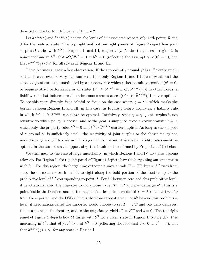
Let breneg( ) and bprohib( ) denote the levels of bD associated respectively with points R and
J for the realized state. The top right and bottom right panels of Figure 2 depict how joint
surplus varies with bD in Regions II and III, respectively. Notice that in each region is
non-monotonic in bD, that d=dbD = 0 at bD = 0 (reecting the assumption c0(0) = 0), and
that bprohib( ) < for all states in Regions II and III.
These pictures suggest a key observation. If the support of around is su¢ ciently small,
so that can never be very far from zero, then only Regions II and III are relevant, and the
expected joint surplus is maximized by a property rule which either permits discretion (bD = 0)
or requires strict performance in all states (bD bprohib max bprohib( )); in other words, a
liability rule that induces breach under some circumstances (bD 2 (0;bprohib)) is never optimal.To see this more directly, it is helpful to focus on the case where = , which marks the
border between Regions II and III: in this case, as Figure 3 clearly indicates, a liability rule
in which bD 2 (0;bprohib) can never be optimal. Intuitively, when = joint surplus is not
sensitive to which policy is chosen, and so the goal is simply to avoid a costly transfer b 6= 0,which only the property rules bD = 0 and bD bprohib can accomplish. As long as the supportof around is su¢ ciently small, the sensitivity of joint surplus to the chosen policy can
never be large enough to overturn this logic. Thus it is intuitive that a liability rule cannot be
optimal in the case of small support of ; this intuition is conrmed by Proposition 1(i) below.
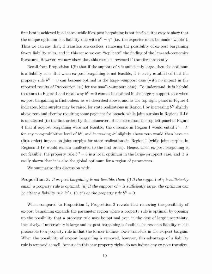
We turn next to the case of large uncertainty, in which Regions I and IV now also become
relevant. For Region I, the top left panel of Figure 4 depicts how the bargaining outcome varies
with bD. For this region, the bargaining outcome always entails T = FT ; but as bD rises from
zero, the outcome moves from left to right along the bold portion of the frontier up to the
prohibitive level of bD corresponding to point J . For bD between zero and this prohibitive level,
if negotiations failed the importer would choose to set T = P and pay damages bD; this is a
point inside the frontier, and so the negotiation leads to a choice of T = FT and a transfer
from the exporter, and the DSB ruling is therefore renegotiated. For bD beyond this prohibitive
level, if negotiations failed the importer would choose to set T = FT and pay zero damages;
this is a point on the frontier, and so the negotiation yields T = FT and b = 0. The top right
panel of Figure 4 depicts how varies with bD for a given state in Region I. Notice that is
increasing in bD, that d=dbD > 0 at bD = 0 (reecting the fact that b < 0 at bD = 0), and
that bprohib( ) < for any state in Region I.
15
The bottom panels of Figure 4 depict the same information for Region IV. In this region, as
the bottom left panel indicates, the outcome always entails T = P ; but as bD rises from zero, the
outcome moves from left to right along the bold portion of the frontier up to a prohibitive level
of bD corresponding to point J . For bD between zero and this prohibitive level, if negotiations
failed the importer would set T = P and pay damages bD; this is a point on the frontier, and so
negotiations implement the DSB ruling T = P and b = bD. For bD at or beyond this prohibitive
level, if negotiations failed the importer would set T = FT and pay zero damages; this is a
point inside the frontier, and so the negotiations lead to T = P and b < bD, and the DSB
ruling is renegotiated. The bottom right panel depicts how varies with bD for a given state
in Region IV. Notice that is (weakly) decreasing in bD, that d=dbD = 0 at bD = 0, and that
bprohib( ) > for any state in Region IV.
Together, Figures 2 and 4 suggest a second key observation: if uncertainty about is large
so that Regions I through IV are all relevant, then a liability rule is optimal. To see this, rst
note that discretion (bD = 0) cannot be optimal. This is because may be raised for states in
Region I by increasing bD slightly above zero which reduces the equilibrium transfer b that the
importer can extract in exchange for FT while joint surplus in Regions II-IV are una¤ected
(to the rst order) by this maneuver. Next note that a prohibitive level of bD cannot be optimal
either: by inspection of Figures 2-4, decreasing bD from a prohibitive level to a level slightly
below strictly improves joint surplus in Region IV (by reducing the equilibrium transfer b
in Region IV that the importer must pay to adopt P ) while not a¤ecting joint surplus in the
other regions. And an immediate corollary of this argument is that the optimal level of bD is
strictly lower than .
With the intuition developed above, we are now ready to state our rst proposition:
Proposition 1. (i) If the support of is su¢ ciently small, a property rule is optimal (speci-
cally, the optimum is bD = 0 if E > and bD bprohib if E < ). (ii) If the support of is su¢ ciently large, the optimum is a liability rule. Moreover, the optimal bD is lower than the
exporters loss from protection: 0 < bD < < bprohib.
We have used the support of as a measure of ex-ante uncertainty. If uncertainty about
is small in the sense of small variance but with a large support, then the optimum will not
be exactly a property rule, but the result will hold in an approximate sense, so the qualitative
insight goes through.
16
Proposition 1 states that a liability rule is optimal only if uncertainty about is large, and
even in this case, the optimal level of damages bD is lower than the level that makes the exporter
whole, i.e. . This result qualies the presumption from the law-and-economics literature
(e.g., Kaplow and Shavell, 1996) that the e¢ cient level of breach damages is the one that makes
the injured party whole; and this qualication arises even under the conditions that are most
favorable to this argument, namely that is known to the DSB. The source of this qualication
comes from our assumption of costly ex-post transfers, and so it applies with particular force
to international dispute resolution. Specically, in the context of the WTO where the damages
paid for breach often take the form of counter-retaliation on the part of the injured party, the
available means of compensation are ine¢ cient, and therefore from an ex-ante perspective they
should not be utilized to an extent that makes the injured party whole. This qualication gains
special relevance in light of the emphasis placed on reciprocity in the GATT/WTO system of
remedies: as noted in the Introduction, it is sometimes suggested that reciprocity falls short as
a mechanism for facilitating e¢ cient breach because it does not make the injured party whole,
but Proposition 1 suggests that this may in fact be a desirable feature of reciprocity.
Moreover, as Proposition 1 indicates, if uncertainty about is su¢ ciently small, any liability
rule is suboptimal (let alone the specic one with bD = ), and instead the optimum is a
property rule. Intuitively, if uncertainty is low and the joint benets of free trade are never
very far from zero, the overriding e¢ ciency concern is to avoid costly transfers; getting the
correct policy choice in each state of the world is secondary. In these circumstances, assigning
a property right to either party provides a disagreement point from which settlement occurs
without transfers, and hence a property rule is preferable to a liability rule.12
Finally, note that Proposition 1 suggests a pair of empirical predictions. First, if uncertainty
about the joint economic/political benets of free trade decreases over time, then the optimal
contractual/institutional arrangement should tend to move away from liability rules and towards
property rules. And second, we should tend to observe more liability rules in issue areas where
uncertainty about the joint economic/political benets of free trade is larger; and conversely,
the use of property rules should be more frequent in issue areas where this uncertainty is smaller.
We next turn to the role of transaction costs in determining the optimal type of agreement.
Recalling that the cost of transfers plays the role of transaction costs in our model, consider
12Recall that property rights are sold ex-post in exchange for transfers only if takes very low or very highvalues (i.e. in regions I or IV), whereas a liability rule induces transfers in equilibrium in any region.
17
an increase in c(b) for all b 6= 0 (while preserving the properties of c(b) that we have assumed),xing the support of . It is clear by inspection of Figure 1 that Regions II and III expand,
while Regions I and IV contract, and at some point Regions I and IV disappear. Using similar
arguments to those presented above, it then follows that when the cost of transfers is su¢ ciently
high a property rule is optimal. Next consider decreasing the cost of transfers: as Figure
1 indicates, Regions I and IV expand, while Regions II and III contract, and as the cost
of transfers goes to zero, the probability of being in Regions I and IV must become strictly
positive. Again using similar arguments to those presented above, it then follows that if the
cost of transfers is small enough, the optimum is a liability rule.
The following proposition states the result:
Proposition 2. (i) If the cost of transfers is su¢ ciently high, a property rule is optimal. (ii)
If the cost of transfers is su¢ ciently small, the optimum is a liability rule.
Proposition 2 implies that a property rule tends to be preferred to a liability rule when
transaction costs are high. This result stands in contrast with the nding in the law-and-
economics literature that liability rules tend to be preferable to property rules when transaction
costs are high (Calabresi and Melamed, 1972, and Kaplow and Shavell, 1996). Our result di¤ers
from this earlier nding because of our focus on the cost of transfers, which as we have indicated
is an important transaction cost in the international government-to-government setting. To gain
further intuition about this di¤erence in results, recall that transaction costs in Calabresi and
Melamed (1972) and Kaplow and Shavell (1996) take the form of bargaining frictions (the
bargain fails with a certain probability); this type of transaction costs penalizes property rules
more than liability rules because property rules induce more bargaining in equilibrium. In our
setting, on the other hand, the presence of a transfer cost penalizes a liability rule more than
a property rule because a liability rule induces more transfers in equilibrium.
Even more surprisingly in light of the Calabresi and Melamed (1972) and Kaplow and Shavell
(1996) nding, we now show that in the presence of a cost of transfers, higher transaction
costs can favor property rules even if these transaction costs take the form of frictions in
bargaining. Specically, we compare the case of frictionless ex-post bargaining (which we have
just considered) with the opposite extreme in which ex-post bargaining is not feasible.
As a preliminary observation, consider what happens if transfers are costless: in this case,
with frictionless ex-post bargaining, liability rules are equivalent to property rules, because the
18
rst best is achieved in all cases; while if ex-post bargaining is not feasible, it is easy to show that
the unique optimum is a liability rule with bD = (i.e. the exporter must be made whole).
Thus we can say that, if transfers are costless, removing the possibility of ex-post bargaining
favors liability rules, and in this sense we can replicatethe nding of the law-and-economics
literature. However, we now show that this result is reversed if transfers are costly.
Recall from Proposition 1(ii) that if the support of is su¢ ciently large, then the optimum
is a liability rule. But when ex-post bargaining is not feasible, it is easily established that the
property rule bD = 0 can become optimal in the large- -support case (with no impact in the
reported results of Proposition 1(i) for the small- -support case). To understand, it is helpful
to return to Figure 4 and recall why bD = 0 cannot be optimal in the large- -support case when
ex-post bargaining is frictionless: as we described above, and as the top right panel in Figure 4
indicates, joint surplus may be raised for state realizations in Region I by increasing bD slightly
above zero and thereby requiring some payment for breach, while joint surplus in Regions II-IV
is una¤ected (to the rst order) by this maneuver. But notice from the top left panel of Figure
4 that if ex-post bargaining were not feasible, the outcome in Region I would entail T = P
for any non-prohibitive level of bD, and increasing bD slightly above zero would then have no
(rst order) impact on joint surplus for state realizations in Region I (while joint surplus in
Regions II-IV would remain una¤ected to the rst order). Hence, when ex-post bargaining is
not feasible, the property rule bD = 0 is a local optimum in the large- -support case, and it is
easily shown that it is also the global optimum for a region of parameters.
We summarize this discussion with:
Proposition 3. If ex-post bargaining is not feasible, then: (i) If the support of is su¢ ciently
small, a property rule is optimal; (ii) If the support of is su¢ ciently large, the optimum can
be either a liability rule bD 2 (0; ) or the property rule bD = 0.
When compared to Proposition 1, Proposition 3 reveals that removing the possibility of
ex-post bargaining expands the parameter region where a property rule is optimal, by opening
up the possibility that a property rule may be optimal even in the case of large uncertainty.
Intuitively, if uncertainty is large and ex-post bargaining is feasible, the reason a liability rule is
preferable to a property rule is that the former induces lower transfers in the ex-post bargain.
When the possibility of ex-post bargaining is removed, however, this advantage of a liability
rule is removed as well, because in this case property rights do not induce any ex-post transfers,
19
whereas a liability rule still does.
Together with Proposition 2, then, our model suggests that higher transaction costs (either
in the form of cost of transfers or bargaining frictions) should tend to favor property rules
over liability rules. This in turn points to an interesting empirical implication: we should
tend to observe more property rules in issue areas where transaction costs are higher; and if
transaction costs rise over time the optimal contractual/institutional arrangement should tend
to move away from liability rules and towards property rules.13
3.2. Noisy DSB investigations
We now turn to the case where the DSB, if invoked, can observe a noisy signal of , which
we denote by . As we mentioned above, here we can consider a wider class of contracts,
where bD can be contingent on . And as we indicated, this scenario is also interesting because
governments are then uncertain about the DSB ruling at the ex-post negotiation stage, and
this has important implications.
We impose a minimum of structure on the signal technology, by requiring that the condi-
tional density of given , denoted h( j ), is log-supermodular. This condition is relativelystandard and is satised by several common distributions (see Athey, 2002). For future refer-
ence, we also let g( j ) denote the conditional density of given .Since at the ex-post negotiation stage governments face uncertainty over what would happen
if the exporter invoked the DSB, the backward induction analysis in this scenario is more
involved than it was under our benchmark scenario. For tractability here we impose a linear
cost of transfers: c(b) = c jbj. The reason this assumption simplies the analysis is that, aswe establish below, the problem of nding the bD schedule that maximizes the ex-ante joint
surplus is equivalent to a simpler problem, namely nding the level of bD that maximizes the
13This suggests an intriguing possibility: if an importing government wishing to increase protection in oneindustry can nd a relatively low-cost way of compensating foreign exporters by o¤ering a tari¤ reduction inanother industry when that tari¤ is set at a high initial level, and can thereby avoid altogether the more costlycounter-retaliation method of compensation, then it could be argued that as negotiated tari¤ cuts become deeperand this maneuver becomes more di¢ cult, the cost of transfers becomes greater and property rules become moreattractive (see Pelc, 2009, note 37 for a related observation). On the other hand, there are other forces thatcut the opposite way: for example, the e¢ ciency costs associated with counter-retaliation itself would be lowerwhen the counter-retaliation begins from tari¤s that are closer to their e¢ cient levels, and for this reason thecost of transfers could fall as negotiated tari¤ cuts become deeper. Also, it is not clear how bargaining frictions(for example stemming from private information) have evolved over time or vary across issue areas. On balance,then, it is di¢ cult to say without further structure how transaction costs might change over time or acrossissues, and so the empirical predictions of our model in this regard remain unclear.
20
expected joint surplus as viewed from stage 4, when the true is unknown, but conditional on
observing a signal . With a nonlinear cost of transfers, this equivalence need not hold, and the
problem is more complex. We leave the analysis of the more general case for future research
(but we believe that our qualitative insights continue to hold).
To state this result, we let 4(bD; ) denote the joint payo¤ in the stage-4 subgame for
a given bD and realized , and we dene the expected joint surplus as viewed from stage 4,
when the realized is unknown, but conditional on observing a signal , as E[4(bDj )] =R4(b
D; )h( j )d . We may now state:
Lemma 1. If c(bD) = c jbDj, then the ex-ante optimal bD( ) maximizes E[4(bDj )].
Armed with Lemma 1, we can now characterize the qualitative properties of the optimal
damages level bD. It is convenient to start with the case of large uncertainty. We assume here
that h( j ) has full support, that is [0;1), for any . We also assume lim !1 Pr( < j ) = 0
(for any xed ): in words, the posterior probability that < approaches zero as the signal
realization becomes innitely large. The following proposition characterizes how the optimal
damages level bD depends on the signal realization and on the (commonly known) exporters
loss from protection :
Proposition 4. Assume h( j ) has full support for any . Then: (i) bD is (weakly) decreasingin , with lim !1 b
D = 0; and (ii) bD is (weakly) increasing in :
According to Proposition 4, the level of damages should be higher when, other things equal,
the signal of the importers gain from protection is lower, or the exporters loss from protection
is higher. Moreover, if the former is very high relative to the latter (i.e., as ! 1 for xed
), the damages for breach that the importer should be required to pay approach zero.
Notice an interesting feature of this result: contrary to the standard logic of e¢ cient breach
whereby damages should reect only the level of harm caused by the breach, Proposition 4
implies that the damages for breach should be responsive to both the level of harm that the
breach causes the exporter and the level of benet that the breach is estimated to provide the
importer. Intuitively, since it is not optimal to set damages at a level that fully compensates
the exporter, making the damages sensitive to the estimated benet that the importer gains
from breach helps to ensure that breach will occur only when it is likely to be e¢ cient.
21
This feature in turn suggests a possible interpretation of the WTO Agreement on Safe-
guards. According to the Safeguards Agreement, an importing government may temporarily
impose tari¤s as a response to injury to its domestic import-competing producers, and need
not compensate the impacted foreign exporters under certain conditions which suggest a more
direct link between the injury and foreign exports.14 If these conditions are interpreted as indi-
cating circumstances in which the imposition of tari¤s would be an e¤ective way of addressing
the injury, then under these conditions the benets of protection to the importer could reason-
ably be thought to be high. And if the DSB receives a signal that this is indeed the case, then
Proposition 4 would suggest that the level of damages should be low or even approach zero,
broadly in line with what the Agreement on Safeguards stipulates in this circumstance.
Next we focus on the case of small uncertainty. We consider two distinct ways in which
uncertainty can be small: rst we consider the case in which there is small ex-ante uncertainty
about , just as in the previous section; and second, we consider the case in which the noise in
the signal is small, so that ex-post uncertainty in (i.e. conditional on ) is small.
Let us start with the case of small ex-ante uncertainty about . It is a simple corollary of
Proposition 1(i) that, if the support of the marginal distribution of is su¢ ciently small, the
optimum is either the property rule bD = 0 or the property rule bD bprohib, with the choicebetween the two contingent on the realized value of the signal .
Next we consider the case in which the DSB information is very precise. If the support
of conditional on is su¢ ciently small, we can apply a logic similar to that which led to
Proposition 1(i) to conclude again that a contingent property rule is optimal, as the following
proposition states:
Proposition 5. If the signal observed by the DSB is su¢ ciently precise, in the sense that the
support of g( j ) around is su¢ ciently small, then the optimum is a property rule (contingenton ).
The analysis of this section suggests two broad implications, one concerning the variation of
optimal rules across issues, and one concerning the evolution of optimal rules over time. Starting14In particular, the Safeguards Agreement species that no compensation need be paid by the importing
government for 3 years when reimposing protection in response to injury of its domestic import-competingindustry, provided that the injury is associated with an absolute increase in imports; whereas if the level ofimports has fallen but the level of domestic production has fallen by more, so that injury is associated withan increase in imports only relative to domestic production, trade protection can still be reimposed but theimporting government must compensate the impacted exporters from the start (in either case, this compensationmay take the form of the temporary withdrawal of equivalent concessions by the exporter).
22
with the cross-sectional implication, our model suggests that the use of property rules should
be more frequent (other things equal) in issue areas where the accuracy of the information that
the DSB can gather ex post is higher, whereas liability rules should be more frequent in issue
areas where the DSB is not likely to be well informed.
Concerning the evolution of the optimal rules over time, our results suggest that, if the
accuracy of DSB rulings increases, the optimal institutional arrangement should move away
from liability rules and toward property rules.15 And as we have previously noted, our model
suggests a similar evolution if ex-ante uncertainty about the joint benets of free trade is
reduced. Thus, if one accepts that the accuracy of legal rulings has increased from the time of
GATTs inception to the creation of the WTO, and/or that the degree of ex-ante uncertainty
about the joint benets of free trade has diminished over this period, then we may ask whether
or not the evolution from GATT to the WTO has indeed been in the direction away from
liability rules and toward property rules. Here opinions di¤er among legal scholars, and we do
not take a stand on the merits of the di¤erent views that have been expressed.16 Rather, we
simply note that the implications of our model suggest plausible circumstances under which
such an evolution would be desirable from an institutional-design perspective.
4. The Outcome of Disputes
In this section we consider the implications of our model for the outcome of trade disputes. To
this end, we rst link more directly the stages of our game with the stages of a WTO dispute.
Broadly speaking, there are three phases to aWTO dispute. In a rst phase, the complainant
must request consultations with the respondent. If consultations fail to settle the dispute within
15Here it is interesting to note that Pelc (2009), who maintains that the GATT/WTO escape clause has shiftedaway from a liability-rule approach towards a property-rule approach, attributes this shift to an improved abilityof the DSB to verify that a legitimate circumstance for escape has arisen, broadly in line with what would beexpected based on our analysis.16On the one hand, Jackson (1997, pp. 62-63) expresses the view that, while the early GATT years were
ambiguous on this point, ...by the last two decades of the GATTs history..., the GATT contracting parties weretreating the results of an adopted panel report as legally binding...,and that the WTO ...clearly establishes apreference for an obligation to perform the recommendation...(emphasis in the original). On the other hand,Hippler Bello (1996) and Schwartz and Sykes (2002) view the changes in the DSB that were introduced with thecreation of the WTO di¤erently. According to Schwartz and Sykes, the GATT was devised to operate accordingto a liability rule that permitted e¢ cient breach, where the penalty for breach in practice took the form ofunilateral retaliation, but in the GATTs nal years unilateral retaliation became excessive and discouragede¢ cient breach. The changes in the DSB that were introduced with the creation of the WTO were motivated,according to Schwartz and Sykes, by a need to reduce the penalty for breach, thus returning the system to onebased squarely on liability rules.
23
60 days of the request, then the complainant may request that a Panel be established. In a
second phase, the Panel gathers information on the dispute and issues a ruling which may be
appealed to the Appellate Body, leading to a nal ruling. And in a third phase, governments
may engage in negotiations over the extent and modalities of compliance with the DSB ruling
(with a compliance panelavailable in case of further disagreements).
Below we seek to develop the predictions of our model, and at a broad level match these
predictions to the various possible outcomes under WTO-like contracts and dispute settlement
procedures. To this end we now o¤er interpretations of model outcomes in terms of observable
outcomes of the WTO dispute settlement procedures.
Let us consider rst the interpretation of stages 2 and 3 in our model. Given that the WTO
DSB requires that governments consultprior to requesting that a formal dispute Panel be
formed for the purpose of issuing a ruling, it is natural to think of the consultation phase of the
WTO dispute settlement process as being reected in a stage 2 negotiation. The interpretation
of stage 3 of our model seems equally straightforward: it is natural to think of a stage-3 ruling
by the DSB as corresponding to the issuance of the Panel/Appellate Body nal ruling.
Next, we turn to the interpretation of stage 4, and in particular the di¤erence between
the outcome where the DSB ruling is implemented and the outcome where the DSB ruling is
renegotiated. In the former case, the DSB ruling denes a disagreement point for the subsequent
negotiations which is on the Pareto frontier, and so there is nothing to gain from renegotiating
the DSB ruling. In the latter case, the DSB ruling denes a disagreement point that is inside the
Pareto frontier, and so in this case renegotiations take place: in particular, the DSB announces
a breach payment under which (i) the home country would prefer to choose P and make the
DSB-mandated breach payment rather than the alternative of FT with no payment, but (ii)
the home country would prefer a third alternative to the two choices under the DSB ruling,
namely, a policy of FT combined with a payment from the exporter. In this light, it seems
natural to interpret a renegotiation that occurs in stage-4 as corresponding to a settlement in
which the appropriate level of compensation is worked out between the disputants prior to the
importer agreeing to bring its policies into compliance by adopting FT .17
17At a broad level, the renegotiation of DSB rulings in our model corresponds roughly to the determination ofa mutually agreed solutionas provided for under Article 3.6 of the WTO Dispute Settlement Understanding(see, for example, the mutually agreed solution to the U.S.-Canada lumber dispute reached on October 12,2006 and notied under Article 3.6). At a more specic level, a good illustration is provided by the compliancesettlement for the U.S.-EU Bananadispute in the WTO (see USTR, 2001). In reaching a settlement for thisdispute, the EU (respondent) stated on April 11, 2001, when the dispute was settled/resolved, that it would
24
4.1. Predictions from the basic model
Having described the broad link from our model outcomes to stages of WTO disputes, we
now return to the formal analysis of our model. There are three possible model outcomes to
consider: (i) Early Settlement, which occurs when the importers o¤er at stage 2 is accepted;
(ii) DSB is Invoked and the DSB Ruling is Implemented ; and (iii) DSB is Invoked but the DSB
Ruling is Renegotiated.18 We focus in this and the next subsection on the case in which the
DSB can observe a noisy signal of , and we keep the assumptions we made in section 3.2.
A rst observation is that, for realizations of in Regions I and IV governments settle early,
while for realizations of in Regions II and III governments go all the way to a DSB ruling.
With this observation, we may state:
Remark 1. Early settlement occurs if is very low or very high, while a DSB ruling is triggered
for intermediate values of .
The arguments that establish the rst part of this Remark are straightforward. Extreme
values of correspond to Regions I and IV, and in these regions stage-2 uncertainty about
the DSBs signal realization (and hence level of damages) does not place the disagreement
point above the Pareto frontier, as the top left and bottom right panels of Figure 5 conrm
(E[D] denotes the disagreement point): as a result, governments have no reason to seek a
ruling. Intuitively, when the joint surplus associated with FT is either very large and positive
or very large and negative, the equilibrium policy choice is independent of the level of damages
determined by the DSB, and so governments have nothing to gain by seeking a DSB ruling.
More subtle is the reason why the DSB is invoked in equilibrium for intermediate values
of . First observe that intermediate values of correspond to Regions II and III, where the
joint surplus associated with FT may be positive or negative but it is moderate in size. For
this reason, the Pareto frontier is convex and the equilibrium policy does depend on the level of
damages determined by the DSB, as the top right and bottom left panels of Figure 5 conrm.
come into compliance with the DSB ruling, but not fully until January 1, 2006. Hence, during this interveningperiod, the United States (a claimant) by accepting the EUs non-to-partial compliance over this period essentially allowed the EU to take some compensation (by being able to unilaterally deviate from its WTOcommitment over this period) in exchange for the promise by the EU to fully comply by January 1, 2006. Wethank Chad Bown for pointing us to this dispute as a suggestive illustration of our specic model result.18By construction, in our model governments always engage in stage-2 consultations,and for this reason, we
focus on the models predictions concerning early settlement and renegotiation of DSB rulings. Our model couldbe extended to consider the issue of whether or not governments initiate consultations; a natural possibility inthis regard would be to introduce a cost of consultation. We leave this extension to future research.
25
The next step is to understand why a convex frontier leads to a DSB ruling in equilibrium.
Graphically, given stage-2 uncertainty about the DSBs signal realization (and hence level of
damages), the disagreement point is above the stage-2 Pareto frontier, as the top right and
bottom left panels of Figure 5 conrm, and hence the importer prefers to trigger a DSB ruling
rather than settle early. To gain a more direct intuition for this insight, consider the extreme
case in which c is innite, so that transfers are not feasible. Then the frontier is made of two
points, P and FT , and any payo¤ combination between those two points is not feasible. In this
case, invoking the DSB brings about an (expected) payo¤ combination that lies between points
P and FT , due to the random nature of the DSB ruling; and since this is the disagreement point,
there is no scope for early settlement. In essence, then, the role of the DSB ruling is analogous
to that of a transfer, in that it makes feasible certain intermediate payo¤ combinations that
would not otherwise be feasible.19
Remark 1 highlights ex-post conditions under which governments either settle early or pur-
sue a dispute through to the ruling stage. But it is also interesting to examine the ex-ante
probability of early settlement versus DSB ruling. To this end, note that Pr(Settlement) =
1Pr(Ruling). Thus we can focus on the determinants of Pr(Settlement), as the determinantsof Pr(Ruling) are mirror images of the former.
If we dene an increase in uncertainty over as a mean-preserving spread of its distribution,
and assume for simplicity that E = , a direct implication of the arguments made above is:
Remark 2. As uncertainty over increases and/or the cost of transfers decreases, the proba-
bility of early settlement increases.
The intuition for Remark 2 is similar to Remark 1, and can be understood again with the
aid of Figure 5. In particular, as long as there is any uncertainty in the DSB ruling, i.e. bD
depends on , there is settlement in equilibrium if and only if falls in Regions I or IV. But
the probability of Regions I and IV combined is higher when is more uncertain and/or when
the cost of transfers is lower, and the result then follows.
19It is worth emphasizing that the prediction that disputes ever proceed to a ruling (i.e., go to court) and hence the ability to make statements about when early settlement is likely to occur distinguishes ourmodel from much of the law-and-economics literature concerned with liability rules versus property rules. Forexample, Kaplow and Shavell (1996) consider the case of a perfectly uninformed and perfectly informed court,but they do not consider the case of an imperfectly informed court (our case of noisy DSB investigations) andso disputes are always settled early in their analysis.
26
We next turn to consider the probability that a DSB ruling is implemented versus renego-
tiated. We focus on ex-post conditions under which rulings are implemented or renegotiated:
Remark 3. Conditional on a DSB ruling being triggered, the ruling is renegotiated when the
DSB-assessed damages bD() fall in an intermediate range, while it is implemented when bD()takes very low or very high values.
The intuition for this Remark is as follows. First, recall from Remark 1 that a ruling is
reached in equilibrium only for realized in Regions II and III. Second, recall that renegotiation
of the DSB ruling occurs when (i) Home would prefer to choose P and make the DSB-mandated
breach payment rather than the alternative of FT with no payment, but (ii) Home would prefer
a third alternative to the two choices under the DSB ruling, namely, a policy of FT combined
with a payment from the exporter. And nally note that, as Figure 6 conrms, for Regions II
and III this occurs for intermediate levels of the damages bD(). Hence, according to Remark3, DSB rulings should be renegotiated when the DSB issues a closeruling, i.e., a ruling that
does not suggest either very high or very low joint surplus associated with the FT policy.
Note also an interesting implication of Remark 3: it may well happen that compliance with
the DSB ruling becomes an issue and the ruling is ultimately renegotiated even though the
DSB ruling gets it right(i.e. is close to ). In other words, our model indicates that the
renegotiation of DSB rulings does not come about because rulings are bad.
4.2. Di¤erential cost of transfers between developed and less-developed countries
As illustrated by Remark 2 above, an interesting feature of our model is that the cost of
international transfers can have important implications for predictions concerning the outcomes
of disputes. If we introduce the further assumption that the cost of granting a (positive) transfer
is higher for less-developed countries than it is for developed countries, then our model generates
predictions for the variation in outcomes that arise when disputes are between two developed
countries, between two developing countries, or between a developed and a developing country.20
Here we consider the models predictions regarding a dispute between a developed and a less-
developed country, assuming that the cost of transfers c is higher for the latter. For this
discussion we also assume for simplicity that the distribution of is symmetric about .
20Horn and Mavroidis (2008) document the interesting variation in outcomes of WTO disputes depending onthe developed/less-developed status of the disputants.
27
We rst observe that, under these assumptions, the model predicts that if the developed
country is the respondent (importer), then with relatively high probability we are in Regions
II or IV. This is because, as can be conrmed by graphical inspection, if the developed country
is the importer then Region II consists of an interval of that is larger than Region III, and
similarly Region IV consists of an interval of that is larger than Region I, owing to the
relatively low (high) cost of transfers for the developed (less-developed) country. On the other
hand, if the less-developed country is the respondent (importer), then the model predicts that
with relatively high probability we are in Regions I or III, for analogous reasons.
These observations carry several implications. First we consider the implications of asym-
metric costs of transfer for the observed outcomes of disputes between developed and developing
countries under early settlement. We may state:
Remark 4. Conditional on the developed country being the respondent, early settlements
result in a policy of P (with compensation paid by the developed country to the developing
country) with probability higher than 1=2. Conditional on the less-developed country being
the respondent, early settlements result in a policy of FT (with compensation paid by the
developed country to the developing country) with probability higher than 1=2.
Thus, according to Remark 4, there is a tendency for developed countries to end up imposing
more protection in equilibrium as a result of early settlements than is the case for less-developed
countries. This Remark follows directly from the fact that if the developed country is the
respondent, then the probability is higher that the realized is in Region IV than that it is in
Region I, and vice versa if the less-developed country is the respondent.
We next consider the outcomes of disputes between developed and developing countries that
proceed all the way to a DSB ruling. We may state:
Remark 5. Conditional on the developed country being the respondent, DSB rulings tend to
occur when < 0, that is, when FT is the rst-best policy. Conditional on the less-developed
country being the respondent, DSB rulings tend to occur when > 0, that is, when P is the
rst-best policy.
Thus, according to Remark 5 there is a pro-trade (anti-trade) selection bias in rulings when
a developed country (less-developed country) is the respondent. This follows directly from the
fact that if the developed country is the respondent, then the probability is higher that the
28
realized is in Region II than that it is in Region III, and vice versa if the less-developed
country is the respondent.
5. Extensions
In this section we consider two extensions of our basic model. We rst extend our analysis to a
richer informational environment, where both and are non-veriable. We then consider a
broader class of contracts, where in addition to a stickassociated with the choice of P (the
damages level), the contract can also specify a carrotassociated with the choice of FT .
5.1. Both and non-veriable
Here we consider a scenario in which both and are non-veriable. In particular, we now
assume that and are ex-ante uncertain and independent of each other, with their ex-ante
(common-knowledge) distributions denoted respectively by h( ) and h( ). Both governments
observe and ex post, while the DSB does not. We also assume that and have the
same support; note that this implies that the support of includes the value = 0.
We focus here on the case in which the DSB receives no information ex post. In this case,
most of the analysis in section 3.1 continues to hold, provided our statements about uncertainty
in are re-interpreted as statements about uncertainty in (so, for example, the case in which
the support of is large should be re-interpreted as the case in which the support of is
large).21 But there is one important exception: in the case of large support of , it may no
longer be that bD bprohib is dominated by some lower level of bD.To understand this point, it is rst helpful to recall why it is that, when is known ex ante
and the support of is large enough so that Regions I and IV become relevant, it cannot be
optimal to set bD bprohib. As our arguments leading up to Proposition 1 indicate, this followsbecause bprohib( ) > for in Region IV but bprohib( ) < for in the other regions, and so
moving from a strict performance rule to a liability rule by decreasing bD from bprohib to a level
slightly below strictly improves joint surplus in Region IV while not a¤ecting joint surplus
in the other regions. But when is also uncertain, this argument can only be made if Region
IV is relevant for some when the realized takes its maximum value. And if the support of
21Our results for the case in which the DSB receives a noisy signal as reported in Propositions 4 and 5 andthe Remarks also generalize to the setting in which both and are ex-ante uncertain, with the one exceptionbeing that bD need not be (weakly) increasing in the signal unless the signal is su¢ ciently precise.
29
is wide enough relative to that of (which is the case under our assumption that and
share the same support), Region IV cannot be relevant when the realized takes its maximum
value; hence this argument does not apply.
As is true when is known ex ante, in the current setting where and are both uncertain,
altering the degree of ex-ante uncertainty and altering the cost of transfers each has a similar
e¤ect on the optimal rules. We therefore have the following result:
Proposition 6. Suppose that the DSB receives no information ex post, and that both and
are uncertain. Then: (i) If the support of is su¢ ciently small, or the cost of transfers is
su¢ ciently large, a property rule is optimal (either bD = 0 or bD bprohib). (ii) If the supportof is su¢ ciently large, or the cost of transfers is su¢ ciently small, the optimum can be either
a liability rule (0 < bD < bprohib) or the property rule bD bprohib.
Two interesting aspects of Proposition 6 should be highlighted. The rst is that the presence
of uncertainty about the exporters loss from protection ( ) further weakens the case for a
liability rule, since now even in the case of large support of a property rule may be optimal.
And the second is that, together with Proposition 1, Proposition 6 and the arguments leading
up to it suggest that the case for a liability rule is strongest when uncertainty is large and the
importer faces asymmetrically large risk (so that most of the uncertainty about is derived
from uncertainty about , not ).
Finally, in light of Proposition 6 it is interesting to revisit the e¤ects of bargaining frictions
in the current setting where both and are uncertain. Recall that, under the assumption
that is known ex ante, a comparison across Propositions 1 and 3 establishes that removing
the possibility of ex-post bargaining expands the parameter region where a property rule is
optimal. However, if both and are uncertain, the introduction of bargaining frictions may
or may not favor property rules. More specically, when and are uncertain it is still true
(as is the case when is known ex ante) that if ex-post bargaining is not feasible, the property
rule bD = 0 can be optimal in the large--support case. But when and are uncertain,
it can also be established that the strict performance rule bD bprohib cannot be optimal in
the large--support case when ex-post bargaining is not feasible,22 which is interesting because,
as Proposition 6(ii) indicates, when ex-post bargaining is frictionless, it is the property rule
22To see this intuitively, consider Figure 4: as the bottom left panel indicates, when ex-post bargaining isnot feasible, setting bD at its prohibitive level simply forces T = FT , and the joint surplus is thereby discretelyreduced, rather than discretely increased as Figure 4 indicates is the case when ex-post bargaining is frictionless.
30
bD = 0 that cannot be optimal and the property rule bD bprohib that can be optimal in thelarge--support case.
This discussion leads to the following point: when both and are uncertain, removing
the possibility of ex-post bargaining tilts the use of property rules away from strict performance
contracts (bD bprohib) and towards discretion (bD = 0). It is not immediately obvious why
bargaining frictions should work in a biased way against strict performance contracts relative to
discretion. After all, while bargaining frictions reduce the opportunities for ex-post negotiation,
this applies whether the ex-post negotiations begin from a position of T = FT (as in strict
performance contracts) or T = P (as in discretion). What accounts for this bias is the fact that
the elimination of ex-post bargaining opportunities pushes for a lower optimal bD, both around
bD slightly above 0 and around bD = bprohib, and this implies that bD = 0 is more likely to be
optimal and bD bprohib is less likely to be optimal when ex-post bargaining is infeasible.
5.2. A More General Class of Contracts
Thus far we have restricted our analysis to a menu contract that gives the importing government
a choice between setting P and compensating the exporting government with a payment bD,
or setting FT . In this section we consider a richer menu contract that allows the importer
to choose between (P; bD) and (FT; bFT ): that is, the importing government is given a choice
between setting P and compensating the exporting government with a payment bD, or setting
FT and making the associated payment bFT . Intuitively, in addition to the stickimplied by
the payment of damages bD > 0 when the importer chooses P , it might be optimal to include
a carrotimplied by bFT < 0 when the importer chooses FT . Notice, though, that the carrot,
like the stick, is an ex-post transfer and hence costly in our model; and so it is not obvious that
ex-ante e¢ ciency would in fact be served by the inclusion of a carrot in the menu contract.
Let us continue to focus on the case (as in section 5.1) where both and are uncertain
and the DSB receives no information ex post, so that bD and bFT must be noncontingent.
Intuition for our ndings can be developed by returning to Figures 3 and 4. Recall that Figure
3 depicts the case in which = 0, which marks the border between Regions II and III. By
inspection of the right panel of Figure 3, if the support of around zero is su¢ ciently tight,
then even with our more general class of contracts it is still optimal to adopt a property rule
which either permits discretion or requires strict performance in all states of the world. But
then, introducing a carrot (bFT < 0) for FT could never be helpful, because it would simply
31
introduce the equilibrium payment of a costly transfer (bFT < 0) which would accompany FT
when FT would have been chosen in equilibrium anyway and no transfer would have been paid.
Now consider Figure 4, which depicts the same information for Regions I and IV. As we have
observed, when uncertainty over is large, these regions also become relevant. And it again
can be veried that when uncertainty over is large the optimal level of bD is strictly positive.
But here, as can be conrmed using the top left panel of Figure 4, o¤ering a carrot (bFT < 0)
for FT can now be benecial, because when the realized lies in Region I the DSB ruling is
then renegotiated less often and the equilibrium transfer paid by the exporting government to
the importing government is smaller as a result.
Noting again that changes in the degree of ex-ante uncertainty and changes in the cost of
transfers have similar e¤ects, the following result conrms the intuition developed above:
Proposition 7. Suppose the DSB receives no information ex post, and consider menu contracts
of the type (P; bD); (FT; bFT ): (i) If the support of is su¢ ciently small, or the cost of
transfers is su¢ ciently large, it is optimal to set bFT = 0, and the optimal level of bD is either
bD = 0 or bD bprohib; and (ii) If the support of is su¢ ciently large, or the cost of transfersis su¢ ciently small, the optimal levels of bD and jbFT j are strictly positive.
According to Proposition 7, if uncertainty over is su¢ ciently small, then there is no gain
in expanding the simple menu contract that we analyzed in previous sections to include the
possibility of a carrot for FT . Intuitively, introducing a carrot induces ex-post transfers in
equilibrium, which are costly, and provides no benets. On the other hand, using a carrot
can help if uncertainty in is large, because in this case costly ex-post transfers occur in
equilibrium, and the introduction of a carrot can then reduce the size of these transfers.23
It is interesting to consider whether this kind of carrot mechanism is observed in actual trade
agreements such as theWTO. On the one hand, when a government agrees to reduce its tari¤s as
23Observe that the contract class we consider in this section is equivalent to a revelation mechanism T (~s); b(~s),where ~s is the importers report of the state of the world s = ( ; ). This is not the most general class ofmechanisms within our game, however. We have focused on contracts whereby only the importer makes a choiceof policy/transfer or an announcement. Theoretically we could do better by setting up some kind of revelationgame that involves also the exporter. For example, suppose that governments simultaneously announce thevalue of s to the DSB and, if the reports are di¤erent, both governments are hit with steep penalties. Clearlythis kind of mechanism can implement the rst best, because it is an equilibrium for the governments to revealthe true value of s. But we believe it is reasonable to abstract from this kind of mechanism, because in realitythe WTO DSB does not have the power to impose penalties on governments for the policies they choose, letalone for the announcements they make. See Maggi and Staiger (2008) for a discussion of self-enforcement issuesin related contexts.
32
a result of a trade negotiation, it typically considers this to be a concession that is only valuable
to it in exchange for similar concessions from other governments. So it is clearly the norm for a
government to receive some form of compensation from other governments when it agrees to a
policy of free trade. According to this observation, the ndings recorded in Proposition 7 could
potentially be interpreted as suggesting a novel role played by the compensations for trade
liberalization that we observe. But when interpreting the carrot jbFT j, it must be rememberedthat this is an ex-post transfer, which is contractually specied to be executed after the state
of the world has been observed as an additional (ex post) reward for contract performance.
This, of course, rules out transfers that are made as part of an ex-ante negotiation. When put
this way, it is less clear that the carrot-for-performance mechanism represented in Proposition
7 can be found along side the stickof damages-for-breach in existing trade agreements.
Overall, then, our consideration of this more general class of contracts raises some interesting
new questions. Nevertheless, it is worth emphasizing that, while it may well be optimal under
some circumstances to include a carrot bFT in the contract, this does not invalidate our results
from earlier sections regarding the optimal level of damages (bD) and the conditions under
which either liability rules or property rules would be most desirable.
6. Conclusion
In this paper, we analyze the optimal design of legal remedies for breach in the context of in-
ternational trade agreements, with a particular focus on the GATT/WTO. Our formal analysis
delivers sharp conclusions concerning the appropriate remedy for breach and optimal institu-
tional design in light of features of the underlying economic and contracting environment. And
our analysis also delivers novel predictions regarding when disputes arise in equilibrium, and
how the disputes are resolved.
In order to preserve tractability and focus on the main points, we have made a number of
strong assumptions, and it is important to extend our results to more general settings. For
example, we have assumed that there is no cost to initiating disputes, but incorporating such
costs into our model could yield some interesting additional predictions concerning the condi-
tions under which disputes arise in equilibrium. Relatedly, introducing asymmetries in the costs
of initiating disputes between large and small countries and/or developed and developing coun-
tries possibly coupled with asymmetries in bargaining power could yield insights regarding
how the design of legal remedies for breach could best serve a heterogeneous membership.
33
We have made the strong assumption that there is no private information possessed by either
government, an assumption that has helped to bring the distinctive features of our analysis
into sharp relief. Allowing for privately informed governments would introduce an additional
transaction cost in the form of a bargaining friction into our analysis; unlike the transfer costs
that we have emphasized, such bargaining frictions are not specic to the international setting
which is our focus, but they are surely important in real-world trade agreements.
Among the most interesting bargaining frictions from which we have abstracted is the pos-
sible hold-up problem that could arise for the government of an importing country under a
property rule, when there are many exporting governments that hold an entitlement to its
markets. As Schwartz and Sykes (2002) have argued, this consideration may be particularly
relevant for the GATT/WTO in light of its nondiscrimination rules, and it weighs in favor of
a liability-rule interpretation of GATT/WTO commitments. A formal analysis of this issue
within our framework would require extending the model to a multi-country setting. We view
this as a particularly important extension that we leave for future work.
And nally, we have assumed that DSB rulings are automatically enforced. This is a strong
assumption, since in reality DSB rulings must be self-enforcing. Extending our analysis to a
setting of self-enforcing agreements is bound to be a complex task, but we can make one simple
point here. Suppose the importing country can in principle choose to deviate from as distinct
from renegotiate the DSB ruling (e.g. choose policy P and make a payment lower than the
DSB-mandated damages bD), but this deviation can be met with a penalty. What is the optimal
size of this penalty? In our model, the answer is simple: this penalty should be prohibitive, i.e.,
su¢ ciently high to deter this kind of breach in any state of the world. Thus, as a normative
matter, our model suggests that the optimal penalties for breach may be non-prohibitive (i.e.,
induce breach in some states of the world) when it comes to breaching a contractually specied
commitment, but should always be prohibitive when it comes to breaching a DSB ruling.
34
7. Appendix
Proof of Proposition 1: As we argued in the text, the equilibrium outcome of the stage-2
subgame is the same as that of the stage-4 subgame, so we can refer to the negotiation
without specifying the stage in which the negotiation occurs. We start by describing how the
outcome of the negotiation varies with for given bD (notice that in the text we adopted a
di¤erent perspective to develop intuition, and described how the outcome of the negotiation
varies with bD for given ). We need to consider separately two cases: bD and bD > :(a) If bD : It is convenient to think of the importer as having two threat points: FT
with no transfer, and P with transfer bD. For a generic value of , only one of the two threat
points is active: the one that gives the importer a higher payo¤. Given bD, there are two
critical levels of , J(bD) and R(bD), with J(bD) < R(bD), such that: (I) for 2 [0; J()], theFT threat point is active, and the outcome is a policy of FT with no compensation paid by
either party; (II) for 2 [J(); R()], the (P; bD) threat point is active, but the DSB ruling isrenegotiated and the governments agree on a policy of FT and a transfer b(bD ) denedimplicitly by bD = bc(b); and (III) for > R(), the (P; bD) threat point is active and theDSB ruling is not renegotiated, hence the importer chooses P and compensates the exporter
with payment bD. Note that, as crosses the level J(bD), the level of compensation jumps
from zero to strictly negative. It can be shown that J(0) = 0 < R(0) < , and that J and R
are increasing functions with J(bD) < R(bD) for bD 2 [0; ) and J( ) = R( ) > .(b) If bD > : In this case, the only change relative to case (a) is that J(bD) > R(bD),
as can be conrmed by graphical inspection. As a consequence, the equilibrium outcome is as
follows: for 2 [0; R()], the FT threat point is active, and the equilibrium outcome is a policyof FT with no transfer; for 2 [R(); J()], the FT threat point is active, but the DSB rulingis renegotiated and the equilibrium outcome is P with a transfer of ; and for > J(), the(P; bD) threat point is active and the DSB ruling is not renegotiated, hence the equilibrium
outcome is (P; bD).
The next step is to derive the level of bD that maximizes the expected joint payo¤, which we
denote E(bD) (with a slight abuse of notation). It is easy to show that E(bD) is di¤erentiable
in bD. We have to distinguish between cases (a) and (b):
(a) If bD , we can write the ex ante joint payo¤ in the following way:
35
E(bD) =
Z J(bD)
0
V (FT )h( )d +
Z R(bD)
J(bD)
[V (FT ) c(b(bD ))]dH( )
+
Z 1
R(bD)
[V (FT ) + c(bD)]dH( )
where V (FT ) v(FT ) + v(FT ), and H( ) is the cdf of . Di¤erentiating, we get
Equation (7.1) can be understood by noting that a small increase in bD a¤ects the equilibrium
outcome through its impact on the active threat point. For < J() a small increase inbD has no e¤ect because in this case the active threat point is FT , which is independent of
bD; for 2 (J(); R()), an increase in bD leads to a reduction in the compensation that theexporter pays in equilibrium (whose initial level is b(bD )), and hence leads to cost savings ofdc(b(bD ))
dbD> 0; for > R(), an increase in bD translates directly into cost savings of c0(bD);
and nally, an increase in bD results in a shift forward of the jumppoint J(bD), which in turn
implies cost savings of J 0(bD) c(b(bD )). The cost changes just described are weighted bytheir respective probabilities (and by the density h(J()) in the case of the jump point).(b) If bD > , we can write the ex ante joint payo¤ as
In this case, an increase in bD has no e¤ect if < J(); it leads to an increase in the equilibriumtransfer if > J(), resulting in a cost increase of c0(bD); and it shifts the jump point forward,which implies cost savings of J 0(bD)[c(bD) c( )].We are now ready to consider the two cases of large and small support of . It is
convenient to start with the case of large support of . It su¢ ces to prove part (ii) of the
proposition for the case of full support, i.e. 2 [0;1). Let us rst show that the optimal bD
36
is strictly lower than . To show this, note rst that the value bD = weakly dominates
all higher values of bD. This can be easily seen from Figure 1: in Region IV, setting bD >
is weakly dominated by setting bD = , and in Regions I-III the joint payo¤ is constant for
bD . Next note from (7.1) that @E@bDjbD= = c0( )(1 H(R( )) < 0 (where we have
used the fact that J( ) = R( )), and hence there is a strict gain from lowering bD below .
Next let us consider whether it can be optimal to set bD = 0. Evaluating (7.1) at bD = 0 and
recalling that J(0) = 0 < R(0), we have dEdbDjbD=0 = c0( )H(0) + @J
@bDc( )h(J(0)): Clearly,
this derivative is positive.24 Part (ii) of the proposition follows immediately.
Let us now consider the case of small support of (around ). To start with, let us focus
rst on the knife-edge case = . Clearly, in this case bD = 0 and bD bprohib( ) both
yield the rst best outcome, and any other value of bD is suboptimal. Moreover, note that the
only other values of bD that yield a joint payo¤ close tothe maximum are those in a right
neighborhood of bD = 0; all other values of bD yield a joint payo¤ that is discretely lower than
the maximum (including those in a left neighborhood of bprohib( ), because there is a jump at
bprohib( )).
Now consider a small support of around , say ( "1; + "2). Focus rst on valuesof bD that are strictly positive but close enough to zero: clearly, for such values of bD we have@(bD; )@bD
< 0 for all 2 ( "1; + "2), and hence no such value of bD can be optimal. Nextfocus on a value of bD that is not close to zero and that is lower than bprohib( "1) (i.e.non-prohibitive for all values of ): such a value of bD is suboptimal, because by continuity
it yields a joint payo¤ that is discretely lower than the maximum, for each value of in its
support. Finally consider a value of bD that is prohibitive for some values of but not for
others, i.e. bD 2 (bprohib( "1); bprohib( + "2)): such a value of bD is clearly dominated by afully prohibitive value, i.e. by bD > bprohib( +"2), because of the jump that occurs at bprohib( ).
This establishes that in the case of small support only a property rule can be optimal. QED
Proof of Proposition 2: Consider increasing c(b) for all b 6= 0 (while preserving the propertiesof c(b) that we have assumed), xing the support of . It is clear by inspection of Figure 1
that Regions II and III expand, while Regions I and IV contract, and at some point Regions I
and IV disappear. With the cost-of-transfers su¢ ciently high so that only Regions II and III
24There is a small loose end here. The point ( = 0; bD = 0) is a knife-edge point, because the importer isindi¤erent between the two threat points. If the indi¤erence is broken in favor of P the term @J
@bDc( )h(J(0))
will appear, otherwise it will not. But the result goes through in both cases.
37
are relevant, it then follows that there are no transfers in equilibrium under the property rules
bD = 0 and bD bprohib, while there are non-zero transfers in equilibrium under a liability rule.But then, the cost of transfers can always be made su¢ ciently high that their cost outweighs
the gain in joint surplus associated with inducing the correct policy choice. More specically,
consider a level bD that is strictly between 0 and bprohib. By inspection of Figure 2 it is clear
that we can make the cost of transfers high enough that this level of bD is dominated in terms
of joint surplus by bD = 0. This shows that the optimum must be a property rule if the cost of
transfers is high enough.
Next consider decreasing the cost of transfers: as Figure 1 indicates, Regions I and IV
expand, while Regions II and III contract, and as the cost of transfers goes to zero, the proba-
bility of being in either of these two regions approaches zero. Using similar arguments to those
presented in the text (with the distinction noted that the probability of being in Regions II and
III approaches zero), it then follows that if the cost of transfers is small enough, each of the
property rules bD = 0 and bD bprohib can be improved upon, and hence it is optimal to adopta liability rule. QED
Proof of Proposition 3: If the support of is small, it can be shown using a similar argument
as in the proof of Proposition 1 that a property rule is optimal. Focusing next on the case of
where we have used the fact that J(bD) = b+ c(bD). Clearly, for bD we have dEdbD
< 0;and
hence the optimal bD must be lower than . Also note that dEdbDjbD=0 = 0 (since c0(0) = 0 and
h(0) = 0), but dEdbDjbD=" < 0, where " is an arbitrarily small but positive value. This establishes
that bD = 0 is a local maximum. It can be shown by examples that the globally optimal bD
can be either zero or positive. QED
Proof of Lemma 1: Consider an arbitrary schedule bD( ). At stage 4 this schedule induces
equilibrium payo¤s (!4( ; ); !4( ; )). Clearly, all of these payo¤ pairs lie on the ex-post
Pareto frontier given , and can be characterized as we have done so above for given and a
level of (and hence bD). Moving back to stage 2, consider the expected payo¤s conditional
on if stage 4 is reached (i.e. if the DSB is invoked). We denote these expected payo¤s as
(E[!4( ; )j ]; E[!4( ; )j ]). In this proof we omit the argument bD from the payo¤ functions,as this should not cause confusion.
38
Let us consider the four possible regions of . With our assumption of a linear cost of
transfers, the ex-post Pareto frontier in each region is now piece-wise linear: in the four panels
of Figure 5 we display the ex-post frontiers for each of the four regions. As before, the shaded
portion of each frontier depicts the range of stage-4 bargaining outcomes that are induced by
varying and hence bD given a representative realized in the respective region. In Regions
II and III, as the top right and bottom left panels of Figure 5 indicate, the equilibrium payo¤
points (!4( ; ); !4( ; )) constitute a convex locus in (!; !) space. This implies that the
expected payo¤ point (E[!4( ; )j ]; E[!4( ; )j ]) , which we label by E[D] in each panel, liesoutside the Pareto frontier for given . As a consequence, there is no settlement at stage 2 for
realized in these regions, and the DSB is invoked. Thus the equilibrium payo¤s at stage 2 are
given by (E[!4( ; )j ]; E[!4( ; )j ]) for realized falling in either Region II or Region III.In Regions I and IV, the equilibrium payo¤ points (!4( ; ); !4( ; )) lie on a single straight
line for given , as the top left and bottom right panels of Figure 5 make clear. This implies
that the expected payo¤ point (E[!4( ; )j ]; E[!4( ; )j ]) lies on the Pareto frontier, as thepoints labeled E[D] in these two panels indicate. And this implies again that the equilibrium
payo¤s at stage 2 are given by (E[!4( ; )j ]; E[!4( ; )j ]):Now let us consider the optimization problem at stage 0. The objective function isE (E[!4( ; )+
!4( ; )j ]), which we can write as follows:Z Z(!4( ; ) + !
4( ; ))h( j )d
h( )d =
Z Z(!4( ; ) + !
4( ; ))h( j )d
z( )d
where z( ) is the marginal density of . Clearly, maximizing the objective boils down to
maximizingR(!4( ; ) + !
4( ; ))h( j )d for each given . QED
Proof of Proposition 4: We start by writing the derivative dE(4j )dbD
. Clearly we can focus on
values of bD that are lower than , and hence we can write E[4(bDj )] as:
dE(4j )dbD
=c
1 + cJ 0(bD)h(J(bD)j )( bD)+ c
1 + c[H(R(bD; )j )H(J(bD)j )]c[1H(R(bD; )j )];
where we have used the fact that c(b(bD )) = c1+c
( bD) given a linear c().We now argue that dE(4j )
dbDis decreasing in when evaluated at the FOC (dE(4j )
dbD= 0).
Note that the rst and second terms in dE(4j )dbD
are positive, while the third term is negative.
Since h( j ) is log-supermodular, as increases, h( j ) increases proportionally more for highervalues of . This implies that as increases the negative term increases proportionally more
39
than the sum of the two positive terms. Coupled with the fact that, when evaluated at the
FOC (dE(4j )dbD
= 0), the negative term is equal in magnitude to the sum of the positive terms,
this implies that as increases, the negative term increases in magnitude by more than the
sum of the positive terms, and hence dE(4j )dbD
decreases. Given that we were starting from an
optimal (interior) level of bD, it follows that the optimal bD decreases with .
The second part of point (i) is a direct consequence of the assumption lim !1 Pr( <
j ) = 0. It is clear that if Pr( < j ) = 0; then bD = 0 is optimal. One can then show
that, if we make Pr( < j ) = 0 slightly positive, the optimal bD is close to (or equal to) 0.To prove that the optimal bD is increasing in , note: (i) J 0(bD) > 0; (ii) R(bD) is increasing
in ; and (iii) H is increasing. It follows that dE(4j )dbD
is increasing in . QED
Proof of Proposition 5: Omitted.
Proof of Proposition 6: The analysis of this case is analogous to the case where only is
uncertain, except that we need to highlight how J() and R() depend on . It is not hardto show that R is increasing in and J is independent of . We therefore write J(bD) and
R(bD; ):
Given that both and are uncertain, we do not need to write two separate expressions
of E for the cases bD > and bD < . Instead, we have a single expression that involves
In the case of small support of , it can be shown using a similar argument as in the proof
of Proposition 1 that a property rule is optimal. That the same result obtains if the cost
of transfers is high enough (holding everything else constant) can be shown with a similar
argument as in the proof of Proposition 2.
Let us focus now on the case of large support of . We evaluate dEdbD
at bD = 0. Recall that
J(0) = 0 and note that h(0) = 0, hence h(J(0)) = 0. And recalling that ddbDc(b(bD )) < 0,
it follows that dEdbDjbD=0 > 0. This implies that the optimal bD is strictly positive, as claimed.
It can be shown by examples that the optimal bD can be either prohibitive or non-prohibitive.
That the same result obtains if the cost of transfers is low enough (holding everything else
constant) can be shown with a similar argument as in the proof of Proposition 2. QED
40
Proof of Proposition 7: It is easy to show that it cannot be optimal to set bD < 0 or bFT > 0,
so we can focus on the case bD 0, bFT 0. To keep the notation more intuitive we think ofthe choice variables as being the absolute transfer levels, bD and jbFT j.We start by describing how the outcome of the negotiation varies with and for given
bD and jbFT j. We need to consider separately four regions in ( ; ) space. Again we can thinkof the importer as having two threat points: (P; bD) and (FT; jbFT j); for a generic value of ,only one of the two threat points is active. Let us dene = J(bD; jbFT j) as the level of suchthat the importer is indi¤erent between the two threat points; as in the case where bFT 0, itcan be veried that J does not depend on . Also, in analogy with the case where bFT 0,let = R( ; bD; jbFT j) denote the level of such that the active threat point is just on theex-post Pareto frontier; this is the border of the region where governments renegotiate. Notice
that (as before) R is increasing in . Finally, let = (bD; jbFT j) be the level of for whichthe curves = J(bD; jbFT j) and = R( ; bD; jbFT j) intersect.Consider now the four relevant regions in ( ; ) space, for given bD and jbFT j: (A) In
the region where < minfJ(); R( ; )g, the (FT; jbFT j) threat point is active, and there isno renegotiation, so the outcome is a policy of FT with the exporter paying jbFT j; (B) Inthe region where J() < < R( ; ), the (P; bD) threat point is active, but the DSB ruling isrenegotiated and the equilibrium outcome is a policy of FT with the exporter making a transfer
to the importer, which we denote b(bD; ); (C) In the region where > maxfJ(); R( ; )g,the (P; bD) threat is active and there is no renegotiation, hence the outcome is a policy of P
with the importer paying bD; (D) In the region where R( ; ) < < J(), the (FT; jbFT j)threat is active, but there is renegotiation and the equilibrium outcome is a policy of P with
the exporter making a transfer, which we denote b(jbFT j; ).We next consider how E depends on bD and jbFT j. Using a similar logic as in the proof of
Let us rst prove Proposition 7(ii). Focus on the case of large support of . A necessary
condition for jbFT j = 0 to be optimal is @E@jbFT j
jbFT j=0;bD=~bD
0, where ~bD is the optimal
value of bD conditional on jbFT j = 0. Recall that ~bD 2 (0;bprohib) when the support of islarge enough. Note that (a) @J
@bD> 0 and @J
@jbFT j > 0; (b) [c(b(bD; )) c(jbFT j)] > 0 and
[c(bD) c(b(jbFT j; ))] > 0; and (c) @@jbFT jc(b(jb
FT j; )) < 0. It is then direct to conclude
that @E@jbFT j
jbFT j=0;bD=~bD
> 0, and hence the optimal jbFT j is strictly positive. With a similarargument one can show that the optimal value of bD is strictly positive.
The claim that the optimal bD and jbFT j are strictly positive if c is small enough (holdingeverything else equal, including a nite support for ) can be shown with a similar argument
as in the proof of Proposition 2.
We can now turn to claim (i) of Proposition 7. We focus on the case of small support of
. Consider rst the knife-edge case = 0, or = : Let us characterize how (bD; jbFT j; )depends on bD and jbFT j. Clearly, there are two sets of points (bD; jbFT j) that are optimal: (i)any pair such that bD = 0 and jbFT j min induces T = P and b = 0, and hence is optimal; (ii)any pair such that bFT = 0 and bD bprohib induces T = FT and b = 0, and hence is optimal.Following a similar logic as in the proof of Proposition 6, we can next ask what other points
(bD; jbFT j) yield a joint payo¤ close to the rst best in this knife-edge case. The answeris: (a) those such that jbFT j min and b
D > 0 is close to zero, and (b) those such that
bD > bprohib(jbFT j; max) and jbFT j > 0 is close to zero. All other pairs (bD; jbFT j) yield a jointpayo¤ that is discretely lower than the rst best.
We are now ready to consider a small support of around 0, say ("1;+"2). Focus rston pairs (bD; jbFT j) of the type (a) described just above. For these pairs, @
@bD< 0 for all
2 ("1;+"2), and hence no such pair can be optimal. Focus next on pairs (bD; jbFT j) of thetype (b) described above; for these pairs, @
@jbFT j < 0 for all 2 ("1;+"2), and hence no suchpair can be optimal. All other pairs must be suboptimal too, because by continuity they yield
a joint payo¤ that is discretely lower than the rst best for all 2 ("1;+"2), whereas weknow that we can achieve a joint payo¤ close to the rst best with, for example, jbFT j = 0 andbD > bprohib. This proves that, if the support of is small enough, it is optimal to set jbFT j = 0and the optimal bD is either zero or prohibitive.
That the same result obtains if the cost of transfers is high enough (holding everything else
constant) can be shown with a similar argument as in the proof of Proposition 2. QED
42
References
Athey, Susan (2002), Monotone Comparative Statics Under Uncertainty," Quarterly Journal
of Economics," vol. CXVII (1): 187-223.
Bagwell, Kyle and Robert W. Staiger (2005), Enforcement, Private Political Pressure and
the GATT/WTO Escape Clause,Journal of Legal Studies, June.
Bagwell, Kyle (2009), Self-Enforcing Trade Agreements and Private Information, unpub-
lished manuscript, Stanford University, February 15.
Baldwin, Richard, Politically Realistic Objective Functions and Trade Policy,Economics
Letters, vol. 24, pp. 287-90, 1987.
Beshkar, Mostafa (2008a),Trade Skirmishes and Safeguards: A Theory of the WTO Dispute