68
BREATHING SPACE HOW TO TRACK AND REPORT AIR POLLUTION UNDER THE NATIONAL CLEAN AIR PROGRAMME
BREATHING SPACE
HOW TO TRACK AND REPORT AIR POLLUTION UNDER THE NATIONAL CLEAN AIR PROGRAMME

BREATHING SPACE
HOW TO TRACK AND REPORT AIR POLLUTION UNDER THE
NATIONAL CLEAN AIR PROGRAMME
Authors: Anumita Roychowdhury and Avikal Somvanshi
Editor: Arif Ayaz Parrey
Cover and design: Ajit Bajaj
Cover image: Vikas Choudhary
Layout: Kirpal Singh
Production: Rakesh Shrivastava and Gundhar Das
© 2020 Centre for Science and Environment
Material from this publication can be used, but with acknowledgement. Maps are not to scale.
Citation: Anumita Roychowdhury and Avikal Somvanshi 2020. Breathing Space: How to track and report air pollution under the National Clean Air Programme, Centre for Science and Environment, New Delhi
Published by: Centre for Science and Environment 41, Tughlakabad Institutional Area New Delhi 110 062Phone: 91-11-40616000Fax: 91-11-29955879E-mail: [email protected] Website: www.cseindia.org
CONTENTS
Chapter 1: Why this study? 7
Chapter 2: Means, methods and lessons—a global perspective 20
Chapter 3: Tracking the rise and fall of air pollution in Delhi 33
3(A): Decoding Delhi’s air quality trends 34
3(B): What Delhi has done and what it still must do 52
References and endnotes 60

6
7
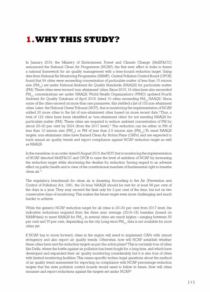
1. WHY THIS STUDY?
In January 2019, the Ministry of Environment, Forest and Climate Change (MoEF&CC) announced the National Clean Air Programme (NCAP), the first ever effort in India to frame a national framework for air quality management with a time-bound reduction target. Using data from National Air Monitoring Programme (NAMP), Central Pollution Control Board (CPCB) found that 94 cities were exceeding concentration of particulate matter of less than 10 micron size (PM
10) set under National Ambient Air Quality Standards (NAAQS) for particulate matter
(PM). These cities were termed 'non-attainment' cities. Since 2015, 16 cities have also exceeded PM
2.5 concentrations set under NAAQS. World Health Organization's (WHO) updated Fourth
Ambient Air Quality Database of April 2018, listed 10 cities exceeding PM2.5
NAAQS.1 Since some of the cities exceed on more than one parameter, this yielded a list of 102 non-attainment cities. Later, the National Green Tribunal (NGT), that is monitoring the implementation of NCAP, added 20 more cities to the list of non-attainment cities based on more recent data.2 Thus, a total of 122 cities have been identified as 'non-attainment cities' for not meeting NAAQS for particulate matter (PM). These cities are required to reduce ambient concentration of PM by about 20–30 per cent by 2024 (from the 2017 level).3 The reduction can be either in PM of less than 10 micron size (PM
10) or PM of less than 2.5 micron size (PM
2.5).To meet NAAQS
targets, non-attainment cities have framed Clean Air Action Plans (CAPs) and are expected to track annual air quality trends and report compliance against NCAP reduction target as well as NAAQS.
In the meantime, in an order dated 6 August 2019, the NGT, that is monitoring the implementation of NCAP, directed MoEF&CC and CPCB to raise the level of ambition of NCAP by increasing the reduction target while shortening the dealine for reduction 'having regard to an adverse effect on public health and in view of the constitutional mandate of fundamental right to breathe clean air.'4
The regulatory benchmark for clean air is daunting. According to the Air (Prevention and Control of Pollution) Act, 1981, the 24-hour NAAQS should be met for at least 98 per cent of the days in a year. They may exceed the limit only for 2 per cent of the time, but not on two consecutive days of monitoring. This makes the future target even more challenging and much harder to achieve.
While the generic NCAP reduction target for all cities is 20–30 per cent from 2017 level, the indicative reductions required from the three year average (2016–18) baseline (based on NAMPdata) to meet NAAQS for PM
10 in several cities are much higher—ranging between 50
per cent and 70 per cent, depending on the city. Long-term PM2.5
data is not available for most cities yet.
If NCAP has to move forward, cities in the region will need to implement CAPs with utmost stringency and also report air quality trends. Otherwise, how will NCAP establish whether these cities have met the reduction targets as per the action plans? This is certainly true of cities like Delhi, where the battle against air pollution has been fought for a long time, and which have developed and expanded their air quality monitoring considerably, but it is also true of cities with limited monitoring facilities. This raises specific techno-legal questions about the method of air quality trend assessment for reporting on compliance with NCAP percentage reduction targets that the state pollution control boards would need to follow in future. How will cities measure and report reductions against the targets set under NCAP?
B R E A T H I N G S P A C E
8
Currently, the CPCB method of reporting annual average data for criteria pollutants from monitors in cities to assess status of compliance has an established protocol for manual monitors in terms of basic data requirement, including the requirement of data of at least 104 days in a year to establish an annual trend and a minimum of 16 hours of data to establish daily averages.5 This is backed by protocol for quality control and assurance. The number of manual stations has increased with time. City average is based on the average of all available manual stations with a minimum of valid 104 days of monitoring. Stations are not included in the computation of the annual average if they do not meet this criteria. Thus, current official construction of annual trend based on manual data needs data for just 28.5 per cent of days in a year.
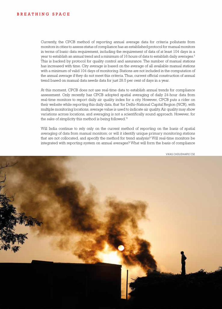
At this moment, CPCB does not use real-time data to establish annual trends for compliance assessment. Only recently has CPCB adopted spatial averaging of daily 24-hour data from real-time monitors to report daily air quality index for a city. However, CPCB puts a rider on their website while reporting this daily data, that 'for Delhi–National Capital Region (NCR), with multiple monitoring locations, average value is used to indicate air quality. Air quality may show variations across locations, and averaging is not a scientifically sound approach. However, for the sake of simplicity this method is being followed.'6
Will India continue to rely only on the current method of reporting on the basis of spatial averaging of data from manual monitors; or will it identify unique primary monitoring stations that are not collocated, and specify the method for trend analysis? Will real-time monitors be integrated with reporting system on annual averages? What will form the basis of compliance
VIKAS CHOUDHARY/ CSE
B R E A T H I N G S P A C E
9
with NAAQS: spatial averaging of all monitors or data from select monitoring locations? There are several questions today.
There are also concerns around data quality and gaps. For instance, several manual monitors do not meet even the minimum data requirements. But reporting on trend and compliance cannot be avoided on the grounds of poor monitoring and lack of quality data. Globally, manual monitors that are subjected to exacting quality control are often treated as primary monitors and collocated real-time monitors are considered as equivalent and used to fill in data for missed days of monitoring.
More importantly, we need methods to address data gaps. Long-term trend analysis is often plagued by asymmetry in data availability and there are concerns around missing data or data gaps. But, at present, India has not adopted any data substitution method to address data gaps. If any manual station falls short of meeting the benchmark for minimum criteria it is rejected. There is no such data availability requirement for real-time monitoring.
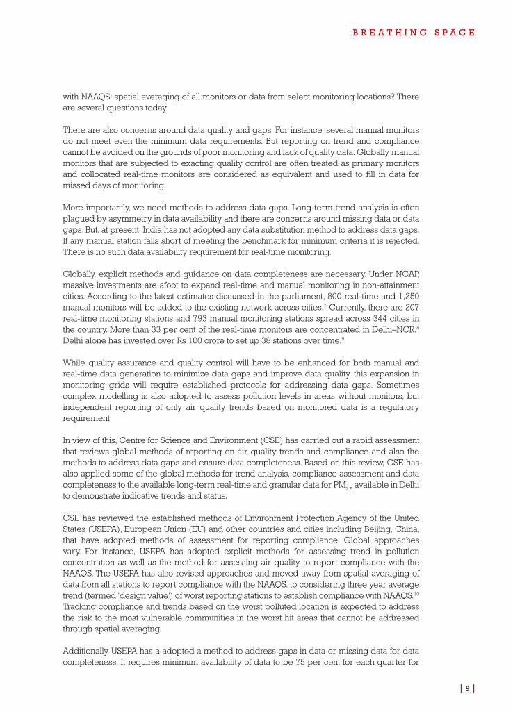
Globally, explicit methods and guidance on data completeness are necessary. Under NCAP, massive investments are afoot to expand real-time and manual monitoring in non-attainment cities. According to the latest estimates discussed in the parliament, 800 real-time and 1,250 manual monitors will be added to the existing network across cities.7 Currently, there are 207 real-time monitoring stations and 793 manual monitoring stations spread across 344 cities in the country. More than 33 per cent of the real-time monitors are concentrated in Delhi–NCR.8
Delhi alone has invested over Rs 100 crore to set up 38 stations over time.9
While quality assurance and quality control will have to be enhanced for both manual and real-time data generation to minimize data gaps and improve data quality, this expansion in monitoring grids will require established protocols for addressing data gaps. Sometimes complex modelling is also adopted to assess pollution levels in areas without monitors, but independent reporting of only air quality trends based on monitored data is a regulatory requirement.
In view of this, Centre for Science and Environment (CSE) has carried out a rapid assessment that reviews global methods of reporting on air quality trends and compliance and also the methods to address data gaps and ensure data completeness. Based on this review, CSE has also applied some of the global methods for trend analysis, compliance assessment and data completeness to the available long-term real-time and granular data for PM
2.5 available in Delhi
to demonstrate indicative trends and status.
CSE has reviewed the established methods of Environment Protection Agency of the United States (USEPA), European Union (EU) and other countries and cities including Beijing, China, that have adopted methods of assessment for reporting compliance. Global approaches vary. For instance, USEPA has adopted explicit methods for assessing trend in pollution concentration as well as the method for assessing air quality to report compliance with the NAAQS. The USEPA has also revised approaches and moved away from spatial averaging of data from all stations to report compliance with the NAAQS, to considering three year average trend (termed 'design value') of worst reporting stations to establish compliance with NAAQS.10 Tracking compliance and trends based on the worst polluted location is expected to address the risk to the most vulnerable communities in the worst hit areas that cannot be addressed through spatial averaging.
Additionally, USEPA has a adopted a method to address gaps in data or missing data for data completeness. It requires minimum availability of data to be 75 per cent for each quarter for
B R E A T H I N G S P A C E
10
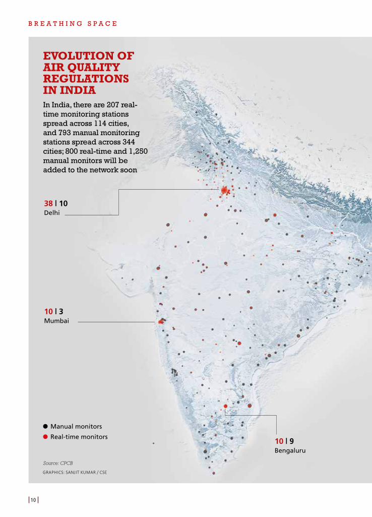
EVOLUTION OF AIR QUALITY REGULATIONS IN INDIA
Manual monitors
Real-time monitors
38 | 10Delhi
10 | 3Mumbai
10 | 9Bengaluru
In India, there are 207 real-time monitoring stations spread across 114 cities, and 793 manual monitoring stations spread across 344 cities; 800 real-time and 1,250 manual monitors will be added to the network soon
Source: CPCB
GRAPHICS: SANJIT KUMAR / CSE
B R E A T H I N G S P A C E
11
The Air (Prevention and Control of Pollution) Act, 1981 was enacted by the Central government with the objective of arresting the deterioration of air quality. The Act mandated the laying down (and annulment) of standards for the quality of air by the Central Pollution Control Board (CPCB). Subsequently, in 1982, the National Ambient Air Quality Standards (NAAQS) were laid down, to
define acceptable levels of various pollutants, mainly nitrogen dioxide (NO2), surface ozone, suspended particulate matter (SPM) and sulphur dioxide (SO2), in the atmosphere. The Standards were revised in 1994 and 1998. In 2009, the Standards were revised again to their current form, which refined standards for SPM into standards for PM of less than 10 micron size (PM10) and standards for PM of less than 2.5 micron size (PM2.5).
National Ambient Air Quality Monitoring Network (later renamed as National Air Quality Monitoring Programme or NAMP) was initiated in 1984–85. Data from NAMP is used to adjudge compliance of urban, industrial and sensitive areas. Traditionally, only manual monitors were available, but real-time monitoring was introduced in India around 2006, initially in Delhi, expanding to several other cities post-2016. However,
even after the introduction of real-time monitors, CPCB continues its practice of using only data from manual monitors to report compliance with NAAQS. It has created a separate
network—Continuous Ambient Air Quality Monitoring Stations (CAAQMs)—for real-time monitors. This network is technically part of NAMP but its data is stored and
treated separately as CPCB has not established method of equivalence between the two monitoring techniques.
NAAQS require two kinds of compliances—daily and annual. To determine annual compliance, the CPCB method requires data of a minimum of 104 days in a year (and at least two days every week). For each such day, monitoring should have been done for at least 16 hours. For urban, industrial or sensitive zones with more than one monitoring stations, data from all stations meeting the CPCB criteria is used to calculate the average, which is then used to
report compliance. As per the CPCB method, data from manual monitors not meeting these criteria is not to be used to report compliance. But CPCB exercises
a bit of discretion on this issue as hardly any manual monitor meets the 104 day data requirement. In the past, CPCB has used data from manual monitors reporting data from
as few days as 50.
The method for calculating daily compliance is the same as the method for calculating annual compliance. Day-wise concentration of pollutants should comply with NAAQS for
at least 98 per cent of the days in a year. Additionally, they cannot exceed NAAQS on two consecutive days of monitoring.
In 2014, the National Air Quality Index (AQI) was established by CPCB. Using NAAQS as the benchmark, it created a grading of ambient air into six categories (seven in Delhi), from good to
severe (severe plus in Delhi), to communicate health risks related to exposure to air pollution. AQI is based exclusively on data from real-time monitors and reports values in the form of a daily AQI bulletin.
Although CPCB does not use data from real-time monitors to report annual NAAQS compliance, it has nevertheless outlined a protocol for real-time monitoring. The protocol outlines the standard parameters for monitoring a list of criteria pollutants and also details meteorological parameters including temperature, wind speed and direction, barometric pressure, solar radiation and rainfall, among others. The protocol asks for 15-minute average values and round-the-clock internet connectivity for data transmission, with an uptime of 99 per cent.
AQI bulletins of the first two years (available only for Delhi) clearly demonstrated the health emergency due to toxic air in the city. The Supreme Court (SC) took note of this and directed CPCB to draw up a Graded Response Action Plan (GRAP) and take other appropriate measures to address different levels of air pollution as per the AQI. The GRAP was promptly notified in 2017 by CPCB under the Environment (Protection) Act, 1986 (EPA), reserving the most stringent (and effective) actions for emergencies and severe pollution episodes and events. Later in the same year, the Environment Pollution (Prevention and Control) Authority, an autonomous statutory body established by the SC under EPA for Delhi–National Capital Region (Delhi–NCR) in 1998, also acting on directions from the SC, issued a Comprehensive Action Plan for long-term redress of air pollution in Delhi. It consisted of multi-sectoral and time-bound actions and assigned clear responsibilities.
It was soon realized that a national plan was needed on the lines of the action taken in Delhi. In January 2019, the Ministry of Environment, Forest and Climate Change (MoEF&CC) announced the National Clean Air Programme (NCAP), the first ever effort in India to frame a national framework for air quality management. However, NCAP goes beyond the approach adopted under the Comprehensive Action Plan in Delhi–NCR (for control of pollution) and introduces time-bound pollution reduction targets.
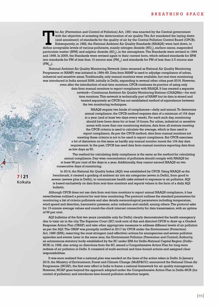
7 | 21Kolkata
B R E A T H I N G S P A C E
12
each station, failing which data substitution tests have to be carried out for data completeness. This codification is very elaborate because air quality trend reporting for compliance with NAAQS is a legal obligation under the US Clean Air Act.
EU, on the other hand, has adopted spatial averaging of all monitoring sites and requires 90 per cent data availability.11 The governments also identify unique primary monitors for reporting trends. Beijing, like Delhi, has about 40 monitoring stations. It has selected 13 monitoring stations for reporting annual trends. China also makes the effort to assess the relative contribution of action against pollution and meteorology to air quality and health gains.12 But these are part of separate specific studies. Clearly, all have a method to report compliance against percentage reduction targets for air quality.
The global review has provided considerable insight into the ways India can consider further elaborations of methods for reporting trends in pollution concentration and for reporting compliance with the stated reduction target and NAAQS. This assessment keeps in view the aspects of data limitations in Indian cities in terms of weak quality control of data, missing and inaccurate data, changing and expanding locations of monitoring and the requirements of reporting compliance.
DEMONSTRATING CHANGE IN DELHI
To make the case for such a change at the national level, CSE has further demonstrated application of global methods to Delhi’s long-term air quality trends and its status vis-à-vis the NAAQS for PM
2.5. Delhi cannot claim—after making such massive investments in monitoring
stations —that it cannot figure out whether its pollution levels are rising or declining. There has to be a way of using available data to understand the indicative percentage change in the trend in concentration and status of compliance with the NAAQS or clean air targets.
There is an additional curiosity about the potential impact of several measures that have been implemented post-2010 on the long-term trend. While it is true that trends are influenced by both short-term and long-term action and meteorology, and several governments do assess this periodically as part of larger scientific assessments, but reporting only trends in concentration based on monitoring data is part of the legal requirement.
At the turn of the new decade, it is important to note that Delhi has witnessed multi-sector interventions to control air pollution during this decade. A series of Supreme Court directives and government interventions have led to several changes in different sectors including industry, power plant, transport, waste and dust. In the industry and power plant sectors, since 2009–10, three power plants have been shut progressively, equalling 1,245 MW of coal power generation.13 Substantial expansion of natural gas has happened in industrial estates.14 An approved fuel list has been notified to ban use of all dirty fuels including pet coke, furnace oil and coal in all sectors.15 Hotspot action in worst affected areas is leading to action on several informal sources of pollution including open burning of industrial waste. Action in industrial hotspots in Bawana and Mundka have led to safe removal of nearly 80,000 tonnes of plastic waste that would have otherwise been burned in the open.16 Nearly half of the brick kilns in Delhi-NCR have adopted the improved zigzag kiln technology.17
In the transport sector, the city has witnessed a rapid renewal of vehicle fleet based on Bharat Stage (BS)-IV norms and the introduction of cleaner BS-VI (10 ppm sulphur fuels) in advance in 2018.18 Truck numbers entering Delhi daily from 13 key entry points have been reduced after the opening of two expressways, imposition of environment compensation charge on truck entry, ban on 10-year old trucks, control on overloading and installation of RFID for cashless
B R E A T H I N G S P A C E
13
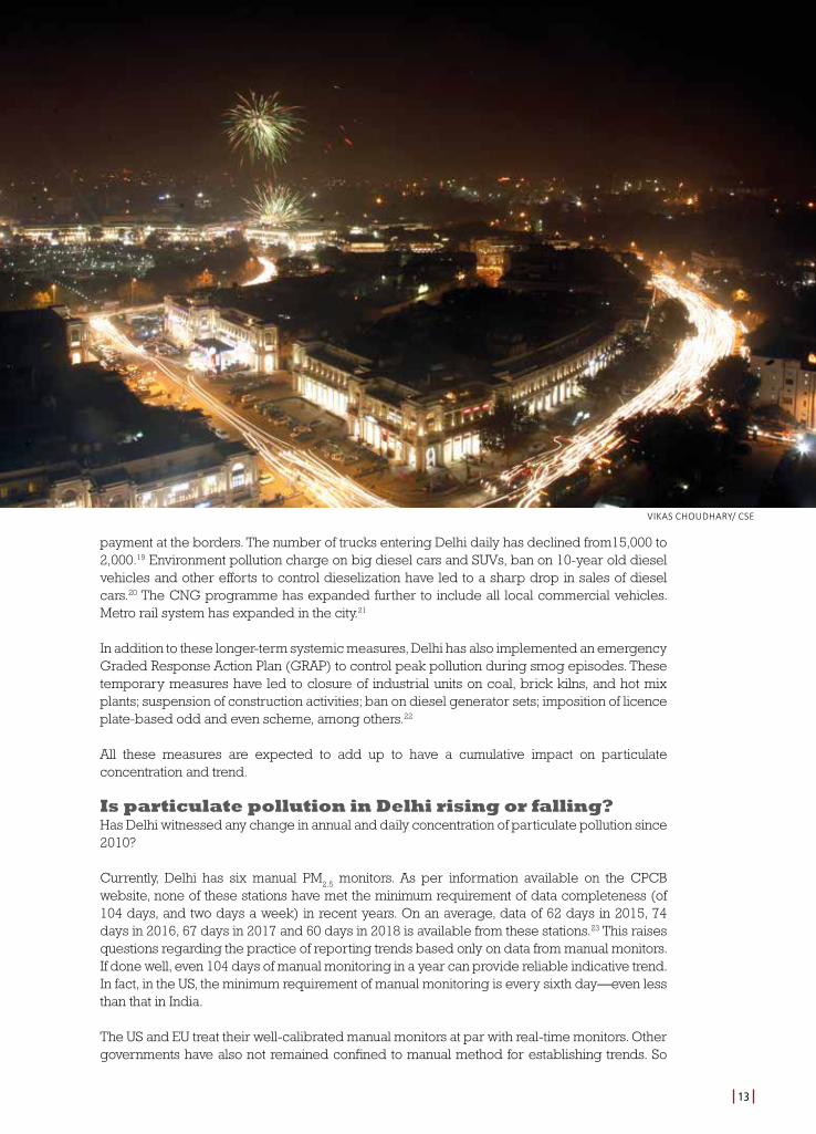
payment at the borders. The number of trucks entering Delhi daily has declined from15,000 to 2,000.19 Environment pollution charge on big diesel cars and SUVs, ban on 10-year old diesel vehicles and other efforts to control dieselization have led to a sharp drop in sales of diesel cars.20 The CNG programme has expanded further to include all local commercial vehicles. Metro rail system has expanded in the city.21
In addition to these longer-term systemic measures, Delhi has also implemented an emergency Graded Response Action Plan (GRAP) to control peak pollution during smog episodes. These temporary measures have led to closure of industrial units on coal, brick kilns, and hot mix plants; suspension of construction activities; ban on diesel generator sets; imposition of licence plate-based odd and even scheme, among others.22
All these measures are expected to add up to have a cumulative impact on particulate concentration and trend.
Is particulate pollution in Delhi rising or falling? Has Delhi witnessed any change in annual and daily concentration of particulate pollution since 2010?
Currently, Delhi has six manual PM2.5
monitors. As per information available on the CPCB website, none of these stations have met the minimum requirement of data completeness (of 104 days, and two days a week) in recent years. On an average, data of 62 days in 2015, 74 days in 2016, 67 days in 2017 and 60 days in 2018 is available from these stations.23 This raises questions regarding the practice of reporting trends based only on data from manual monitors. If done well, even 104 days of manual monitoring in a year can provide reliable indicative trend. In fact, in the US, the minimum requirement of manual monitoring is every sixth day—even less than that in India.
The US and EU treat their well-calibrated manual monitors at par with real-time monitors. Other governments have also not remained confined to manual method for establishing trends. So
VIKAS CHOUDHARY/ CSE
B R E A T H I N G S P A C E
14
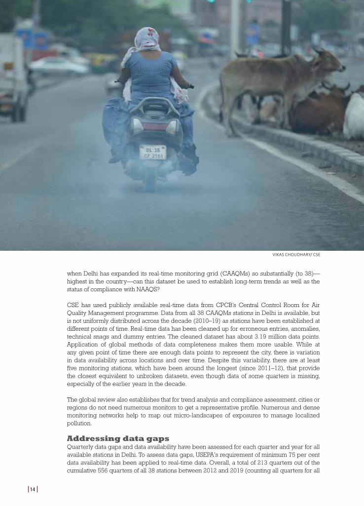
when Delhi has expanded its real-time monitoring grid (CAAQMs) so substantially (to 38)—highest in the country—can this dataset be used to establish long-term trends as well as the status of compliance with NAAQS?
CSE has used publicly available real-time data from CPCB’s Central Control Room for Air Quality Management programme. Data from all 38 CAAQMs stations in Delhi is available, but is not uniformly distributed across the decade (2010–19) as stations have been established at different points of time. Real-time data has been cleaned up for erroneous entries, anomalies, technical snags and dummy entries. The cleaned dataset has about 3.19 million data points. Application of global methods of data completeness makes them more usable. While at any given point of time there are enough data points to represent the city, there is variation in data availability across locations and over time. Despite this variability, there are at least five monitoring stations, which have been around the longest (since 2011–12), that provide the closest equivalent to unbroken datasets, even though data of some quarters is missing, especially of the earlier years in the decade.
The global review also establishes that for trend analysis and compliance assessment, cities or regions do not need numerous monitors to get a representative profile. Numerous and dense monitoring networks help to map out micro-landscapes of exposures to manage localized pollution.
Addressing data gapsQuarterly data gaps and data availability have been assessed for each quarter and year for all available stations in Delhi. To assess data gaps, USEPA's requirement of minimum 75 per cent data availability has been applied to real-time data. Overall, a total of 213 quarters out of the cumulative 556 quarters of all 38 stations between 2012 and 2019 (counting all quarters for all
VIKAS CHOUDHARY/ CSE
B R E A T H I N G S P A C E
15
stations), or 38 per cent of all quarters, have data availability of less than 75 per cent. About 62 per cent have more than 75 per cent availability. But there is variation in distribution.
In view of this variability, this analysis has considered the five oldest stations in the city—IHBAS, ITO, Mandir Marg, Punjabi Bagh and RK Puram—that have the most continuous data since 2012 for long-term trend analysis. Composite averages of these stations have been considered for constructing long-term trends for Delhi. In relation to the USEPA criteria, data availability is over 75 per cent in at least half the quarters (83 out of total of 160 quarters) between 2012–19 (counting all quarters for each stations). Data is available for most quarters. Data from the few quarters that do not meet the 75 per cent data availability benchmark can still be used after employing data substitution methods. One big gap on the CPCB portal is the missing data of 15-minute granularity for the year 2014–15 for the stations Mandir Marg, Punjabi Bagh and RK Puram. Therefore, to crosscheck, data of one-hour granularity was accessed directly from Delhi Pollution Control Committee (DPCC) and this improved the number of quarters with improved data availability to 95. However, as this is a different dataset, estimates have been done with and without it to crosscheck the variability. When the trend is reassessed for these stations using this additional data, the difference is within 5 per cent of the trend analyzed without it.
If the data is examined from the 15-minute granularity angle, 99.4 per cent of 15-minute timestamps in the period from 1 January 2012 to 31 December 2019 have a valid data entry from at least one of these five stations. The missing timestamps (1,728 out of 280,512) are in the second and third quarter of 2012 where availability is 89 per cent and 90 per cent respectively.
Even with data gaps, overall data availability of real-time stations is much better than that of the manual stations. Under the best case scenario, manual data can represent air quality of 28.5 per cent days in a year; 436 of the real-time 556 quarters (79 per cent) meet this requirement.Data (of 2018) from the five stations also correlates better, showing that we are on the right path. ITO and Mandir Marg have highest correlation (0.81) while IHBAS and Punjabi Bagh are least correlated (0.60). The distance between these station pairs can be used to explain the difference in correlation coefficient. But these variations are not high enough to establish presence of unique atmospheric chemistry within Delhi. Subject to more research, these variations can be attributed to pollution from nearby sources instead of variation in wider ambient air of the area. Data from newer stations correlates even better—JNL Stadium, National Stadium, Okhla Phase 2 and Sri Aurobindo Marg stations have a correlation coefficient of 0.9 or higher. USEPA generally applies a 'collocation factor' and considers station pairs with correlation coefficient higher than 0.75 as collocated, treating the data from the collocated station with lower annual average as redundant.
Another long-term trend has been constructed based on the location reporting the worst pollution in the city in a given year (based on three year average level). This aligns with the current USEPA method for reporting compliance with NAAQS. In this analysis, IHBAS station shows up consistently as the worst polluted between 2012 and 2016. Data availability at IHBAS is also better than other stations—13 out of 20 quarters between 2012 and 2016 have 75 per cent availability. Since 2016, the overall data availability for all stations has improved. Data availability is very good for 2018 and 2019, out of 284 quarters, only 12 have less than 75 per cent data availability and just one has less than 26 days of data available.
Issues related to data completenessTo overcome the limitation of data gaps, especially for the earlier years in the decade, the USEPA method of data completeness has been applied as it is the most detailed. To determine the appropriateness and ensure proper application of this method to Indian data, CSE consulted air pollution scientists of USEPA.
B R E A T H I N G S P A C E
16
The scientists affirmed that CSE had accurately applied the USEPA method for minimum data availability and data completeness requirements to Indian (Delhi) data. But the adoption of the method is not without a few caveats.
First of all, when India develops its own method for data completeness, it may change some of the threshold requirements for data availability and completeness. That may have a bearing on results. Given that the sampling requirement in the US is once every six days, technically 12 samples or 12 days of data in a quarter also meet the 75 per cent data completeness threshold. Due to stronger quality assurance and control in the US, actual data availability is of a higher order. On the other hand, since continuous monitors record data everyday, lower data completeness threshold might still be valid.
The second caveat is that in places with large temporal variability (as is the case in India), more valid samples may be needed per quarter in order to characterize the mean with low uncertainty. A statistical test on the locations with more complete datasets is needed to establish exactly what the threshold should be for India.
Yet another caveat is regarding missing data. USEPA has detailed protocols and methodologies to overcome data gaps and address issues with data completeness when the threshold is not met to enable comparison with NAAQS. Missing data can be substituted by the lowest quarterly value (from the preceding or succeeding two years), to test if the three year average of a station exceeds NAAQS, or substituted by the highest quarterly value, to test if the design value (three year average) is below NAAQS. This replacement is to test compliance in reference to the standard, and the average values arrived at after replacement are termed as the test design value (TDV), while the official average of that station remains the one arrived at without replacement. This is because both tests either systematically overestimate or underestimate pollution levels. For the official average, the original average without replacement (but validated by the substitution test) is used. If the missing data is considerably higher, other replacement strategies like mean or median of available valid data can be used to establish the official number.
The methodology for data substitution in the 40 CFR Part 50 of USEPA also works for large data gaps spanning over multiple quarters. In such cases, data from two consecutive years is used to carry out the substitution test. It was recently done for the Corcoran air monitoring station in the San Joaquin valley district of California. The Corcoran station was destroyed in February 2015 and the new monitor could only be installed in the fall of 2016. USEPA used the three year average calculation methodology described in 40 CFR Part 50 and found that the DV for Corcoran station was valid despite the missing 2015 data.24
Another caveat is regarding the selection of stations to be representative of a region or city. USEPA has identified certain stations to be long-term primary station. These stations are designed to represent average conditions across the area, rather than pollution from nearby sources. Doing so also ensures minimal overlap among the monitors in an area being represented by each long-term trend station. In India, there is a clearly defined protocol for location of monitoring stations, but no long-term primary stations for trend analysis.
USEPA also looks at collocation of air quality monitors as stations in close proximity normally yield identical trends. There are elaborate rules on this. Delhi’s real-time monitoring stations are highly correlated in their reported air quality with an average correlation coefficient of 0.77 for every possible pair of stations. Given the unhindered plain topography and distance between stations, the little variation that is present among the stations can also be attributed to pollution from nearby sources. USEPA generally considers station pairs with correlation coefficient higher
B R E A T H I N G S P A C E
17
than 0.75 as collocated and treats data from the station with lower average as redundant.25 Taking this aspect of Delhi’s air quality monitoring network into consideration, spatial averaging of any number or combination of the stations at any given time would essentially yield a similar city average if that data is controlled for isolated episodes and outliers.
Spotlight on DelhiAfter cleaning up the dataset for Delhi, it has become possible to assess the long-term trends in PM
2.5 concentration, seasonal variations, changing pattern of winter pollution and locational
variations more reliably.
Long-term trend analysis of Delhi keeps in view the distinction that the USEPA makes between such analysis and assessment for compliance with NAAQS based on trends in DV. While the city’s compliance with NAAQS is determined by considering the worst station among all the primary monitoring stations, the air quality trend is determined by the composite average of all the designated long-term trend stations. USEPA uses the composite averages among the trend sites in each area to establish and report trends in air quality at each level—city (urban agglomeration), region and national.
Regarding long-term trend analysis, USEPA notes of 2019 on Air Quality Statistics by City explain that the values shown for trend analysis are the composite averages among trend sites in each area.26 Data from exceptional events is included. These trends are based on sites having an adequate record of monitoring data during the trend period. Even for trend analysis three year rolling averages have been considered.
iStock
B R E A T H I N G S P A C E
18
On the other hand, USEPA’s note on compliance of cities with the standard as given in the PM
2.5 Design Values report of 2019 states that the DV for annual PM
2.5 NAAQS is the three year
average annual mean concentration and this is taken to assess compliance with the NAAQS.27
DV must be valid (i.e., meet minimum completeness criteria using the Federal Reference Method—FRM—or equivalent data). For compliance with NAAQS, USEPA considers the worst station in a given year based on its three year average. This is primarily because trends in the worst polluted stations help address issues of vulnerable communities that otherwise get lost in spatial averaging. Addressing the trend in worst polluted stations helps reduce risk for all. Accordingly, the assessment for Delhi includes composite spatial averaging. The second assessment is based on the trend in worst polluted stations. Both trends consider the three year average approach.
The trend analysis based on spatial averaging of five oldest operating stations—considering they represent the air quality of the city and not any specific station— shows over 25 per cent drop between the three year average baseline of 2012–14 and 2016–18. This indicates that the city requires yet another 67 per cent cut to meet the NAAQS for PM
2.5.
When the trend is assessed based on the three year average of the worst monitoring site in a given year—as per USEPA’s current method for assessing compliance with NAAQS—the reduction for the same period increases to 34 per cent. While high gross pollution may show higher decline, the next big target based on worst stations is also high—as much as 75 per cent to meet the NAAQS for PM
2.5.
These results are indicative and may change with changes in threshold values and methods, but these findings are consistent with the trend based on real-time data analysis reported by the System of Air Quality Forecasting and Research (SAFAR) of the Indian Institute of Tropical Meteorology (IITM) under the Ministry of Earth Sciences in India. SAFAR analysis, based on the trends in annual averages since 2012 (in the data obtained from IITM monitors, which are a subset of Delhi's overall real-time monitoring network), bears out that PM
2.5 levels peaked in
Delhi in 2014 and have dropped by about 20 per cent between 2014 and 2019.28
CSE analysis further brings out that due to overall reduction in annual average pollutant concentration, the number of cleaner days has also increased by almost 50 per cent between 2016 and 2019. The number of days meeting daily NAAQS was 68 in 2016, doubling to 120 in 2019. But the number of days with 'severe' pollution have remained unchanged (crawling down to 36 in 2019 from 40 in 2016) and seems to be influenced by regional smog episodes, especially in winters.
Winter smog is also changing its characteristics. The last two winters show delay in setting in of intense winter pollution and also its early tapering off. Peaks during smog episodes are still very high and influenced and aggravated by regional inversion and trapping of pollution. This analysis has also allowed us to establish trends in local pollution, especially to understand hotspots inside the city that need special attention.
MAKE IT HAPPEN
This study has tried to answer specific techno-legal questions about the way Indian cities and regions under NCAP will need to report air quality trends for compliance with NCAP targets and NAAQS. Additionally, it has also demonstrated the application of global methods for such trend analysis and data completeness to Delhi’s real-time data to indicate the direction of change in PM
2.5 concentration trends in Delhi, impact of action, and the direction of future
action. It has yielded many important lessons for NCAP and city administrations.
B R E A T H I N G S P A C E
19
Based on this review, CSE strongly recommends that immediate steps be taken to revisit the current practice of reporting air pollution trends and establish detailed methods for compliance and trend analysis be established, and remedies for data incompleteness be provided.
However, several other steps will be needed to model action plans for estimating their contribution to emerging trends, impact of meteorology on trends and effectiveness of action plans to meet targets. These steps will have to be supported by emissions inventories and source apportionment studies and satellite-based air quality assessment. The litmus test is the implementation of the CAPs to achieve verifiable improvement to meet air quality standards. Each city will be required to do this exercise to understand the direction of change and what is needed for the next big curtailment of pollution. Moreover, only city-based action will not suffice. NCAP will require an appropriate framework for regional action for multi-sector interventions.
Delhi presents an important learning curve for other cities. Multi-sectoral measures implemented in Delhi are not meagre. They have contributed towards stabilization and bending the PM
2.5
curve downwards by over a quarter since 2012. Yet, Delhi is still struggling—and hard—for the next big reduction (of 67–75 per cent) to meet NAAQS.
But yawning gaps in action remain unaddressed. These include massive cuts in emissions from explosive motorization with the help of real-world emissions control for on-road vehicles; integrated multi-modal transportation strategies; vehicle restraint measures like parking policy and zero emission mandate to scale up electric mobility; massive transition from coal to clean fuel across the region; implementation of power plant emissions standards; control of fugitive emissions from small-scale and illegal industrial units, subversive use of dirty industrial fuels, and burning of industrial waste; a paradigm shift in municipal governance vis-à-vis all streams of waste (municipal solid, plastic and e-) to prevent burning; elimination of household use of solid fuels; controls on dust blowing from construction and roads; monitoring and reporting of episodic emissions from crop fire and pollution from outside; are some of the steps needed.
The bigger message for other cities is that none of these measures were easy to implement in Delhi. They were strongly contested in the Supreme Court or opposed in the public domain, delaying deeper and more uniform multi-pronged action. Yet all these hotly contested measures achieved only a little. We can only imagine how tough the next generation action has to be to achieve another 67–75 per cent improvement in Delhi’s air quality. Delhi cannot lose more time fighting against the resistance to solutions. It is high time we deepen our understanding of next generation of measures for clean air while making air quality management more science and data driven.
B R E A T H I N G S P A C E
20
2. MEANS, METHODS AND LESSONS—A GLOBAL PERSPECTIVE
India is expanding its air quality-monitoring grid under NCAP. The expansion is expected to strengthen local databases on air quality, allow assessment of baselines and improvements over time, and support assessment of sources of air pollution and studies on impacts on health. Although the basic objective is grid expansion and optimization for generation of credible data, adopting the desired method for reporting on annual trends and compliance with NAAQS needs immediate attention.
LEVERAGING AIR QUALITY MONITORING GRIDS
With the expansion of the monitoring grid under NCAP, India will begin to generate voluminous data—both manual and real-time—across cities. This data should start feeding the trend analysis process. Resource constraints have prevented establishment of a dense grid in most cities. As of now, there are 793 manual monitoring stations covering 344 cities and 207 real-time monitors covering 114 cities. India has 5,000 cities and towns and larger regions to monitor.
There really are no universal rules for designing monitoring networks. Instead, the stated goals of monitoring in a country dictate the design. Monitoring guidelines provide basic criteria for the minimum required number of monitoring stations and are influenced by varying parameters including population distribution, mixed emissions distribution over complex terrain, different types of sources distributed in the urban area, local meteorological conditions and topography that affect the dispersion of pollutants, among others. Globally, more monitoring stations are recommended in areas with higher levels of pollution and the type of pollutant monitored.
Cities need monitoring systems to provide sufficient information. Measurements taken need to be adequate and representative of air quality conditions of the area.
Grid size also depends on the resources available and programme objectives. As per the World Health Organization (WHO), monitoring systems and programmes also need to be cost-effective, have stable financial, operational, and personnel resources, and be adjusted to local needs and conditions.29 This is an enormous constraint in India, where the mere establishment of a proper real-time regulatory monitor can cost upto Rs 3 crore.
In India, the minimum requirement of number of monitoring stations—pollutant-wise and population-wise—has been established. In order to generate a representative profile of air quality, authorities are expected to focus on different land uses for data generation that include residential areas, industrial locations, traffic areas and background sites. Even though land-use representation is available, background monitors are not available to indicate the minimum pollution possible in the stated region, and to understand maximum reduction possible at any given point of time. CPCB also defines sensitive areas for monitoring and these include health centres, biosphere reserves, national parks, archaeological monuments, etc.
Applying the CPCB recommendation of minimum monitoring based on population, the number of stations in Delhi comes closest to meeting the criteria. Other cities fall substantially short of the population criteria set by CPCB. The number and type (manual and real-time) of
B R E A T H I N G S P A C E
2121
stations and data availability are highly variable over time and across cities. Currently, Delhi has the maximum number of real-time monitors (38). India's six megacities need at least 23 to 44 stations each, while the existing numbers of stations range between nine to 12. In many cities, the number of monitoring stations is bare minimum. Currently, 20 per cent of real-time monitoring infrastructure is catering to less than 2 per cent of population and 0.05 per cent of landmass of India represented by Delhi.
In designing their monitoring network densities, other countries take into account the fact that different pollutants pose different health risks, and concentrate on the gravest threats. In many Western countries, the health effects of NO
2, ozone and PM are grave concerns, therefore
their monitoring has expanded. But concentration of SO2 and airborne lead has declined
substantially everywhere except in some industrial locations. Consequently, the number of stations monitoring these pollutants have been reduced, except in industrial hotspots. Similarly, in most parts of the world, including India, total suspended PM is not monitored any longer, as the tinier fractions (PM
10 and PM
2.5) are considered the bigger health threats.
The global review also shows that for the purpose of regulatory trend analysis, large numbers of monitors are not considered. For instance, New York City has nine PM
2.5 monitoring stations.
Bronx, Brooklyn, Manhattan, Queens and Staten Island have two, one, three, two and one station(s) respectively. Per CPCB’s population criteria, New York City would need 26 PM
2.5 monitoring
stations. The lesser number could also be explained by abating PM2.5
levels in the city. Location of stations is determined by upwind and downwind direction along with other topographical features and not by population (Brooklyn, the most populated borough of the city, has only one station).30 Similarly, San Francisco has just one PM
2.5 station as it is a part of a larger Bay Area
Network and one station was deemed enough to cover air quality of the geographical extent of the city.31 Even if higher pollution levels may merit more stations, the grid will require different scientific criteria to generate representative data to profile a city or a region.
ADDRESSING DATA QUALITY ISSUES IN INDIA
Reliability and accuracy of data from manual monitors is dependent on the calibration status of monitoring instruments, proper sample collection and chemical analysis, and handling by skilled and experienced personnel. Way back in 2003, CPCB, in its National Ambient Air Quality Status report, stated that, ‘[M]onitoring data should be considered indicative and not absolute.’32 Since then, CPCB has initiated auditing of instruments and systems. This process needs to be strengthened under NCAP.
Expansion of the real-time monitoring grid, on the other hand, is a more recent phenomenon. A separate monitoring protocol for real-time monitoring has also been outlined for state pollution control boards (SPCBs). The protocol outlines the standard parameters for monitoring a list of criteria pollutants and also details meteorological parameters including temperature, wind speed and direction, barometric pressure, solar radiation, and rainfall, among others. The protocol asks for 15-minute average values and round-the-clock internet connectivity for data transmission with an uptime of 99 per cent.33
But real-time monitors are not immune to quality compromises. Online datasets require cleaning in terms of inaccurate values that are extremely high or very low and inconsistent with the collocated monitors. Archival and current datasets have several issues. Data is not checked for errors and validated for accuracy. The format is not consistent across stations, for example, methods of rounding off decimal values vary. Meta-data descriptions are missing. There is no noting down or flagging of abnormal events or technical glitches. Data points are missing, which is an impediment for building a proper time series.
B R E A T H I N G S P A C E
22
These concerns will have to be addressed very aggressively as trend reporting becomes a requirement under NCAP. Given the concerns around data gaps or missing data, SPCBs must have a method to deal with data gaps to assess air quality trends. Data gaps at some stations cannot be an excuse anymore to claim that air quality trends for compliance based on more granular data from the ever-expanding air quality monitors cannot be reported under NCAP.
TOWARDS ASSESSING COMPLIANCE
Against the stated NCAP target of 20–30 per cent reduction by 2024 from 2017 levels (or even tighter targets to comply with NGT orders), cities will soon be required to report annual air quality trends and increase in the number of cleaner days, forcing them to delve into several issues.
Currently, CPCB reports annual data on criteria pollutants based on spatial averaging of data from all manual monitors. Nearly all manual stations are treated as primary stations and spatial average of these stations are considered for assessing trends. As per the NAAQS notification, for compliance reporting, city averages are based on the average of all stations with valid annual averages (104 days of monitoring) and minimum 16 hours of valid data that is well distributed over day-time and night-time. In addition, CPCB has a method of classifying cities based on their annual averages to indicate the status of air quality.
CPCB does not consider real-time data in the analysis of annual trends for compliance with NAAQS. Real-time data is considered only for 24-hour average reporting (wherever available) to assess the Air Quality Index of cities, for instance, in Delhi–NCR. But CPCB puts a caveat (while reporting the daily data online) to the effect that, 'Air quality may show variations across locations, and averaging is not a scientifically sound approach. However, for the sake of simplicity, this method is being followed.'34 CPCB does carry out limited analyses of real-time data for reporting daily maximum and minimum in their annual reports.
It is time that the issues of trend and compliance assessment be revisited. Should NCAP continue to rely on simple spatial averaging of only manual monitors? How will the ever-expanding monitoring grid of real-time monitors be integrated with the network of manual monitors? More importantly, how will the minimum requirement of real-time data availability, and the problems of missing data or data gaps be addressed to construct trends and compliance with NAAQS?
GLOBAL LEARNING CURVE
This has made a review of global reporting methods essential. In the US, EU and other countries and regions, there are established methods to scientifically establish trends that do justice to assessing time-bound changes and equitably reducing exposures of vulnerable communities in cities and regions. We have done such a review, but confined it to PM, which is the major concern in India.
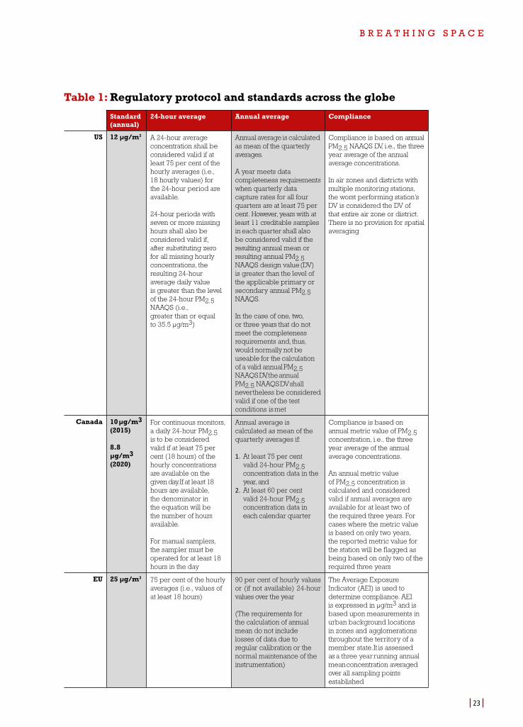
The review found that there are several approaches to perform air quality trend analysis. Many methodologies to establish daily, annual and longer-term pollution concentration trends for cities and regions exist. Countries have varying regulatory protocols regarding safe standards, averaging time, data completeness, standard compliance, data substitution and processes for dealing with missing data and outliers (see Table 1: Regulatory protocol and standards across the globe).
B R E A T H I N G S P A C E
23
Table 1: Regulatory protocol and standards across the globe
Standard (annual)
24-hour average Annual average Compliance
US 12 µg/m3 A 24-hour average concentration shall be considered valid if at least 75 per cent of the hourly averages (i.e., 18 hourly values) for the 24-hour period are available.
24-hour periods with seven or more missing hours shall also be considered valid if, after substituting zero for all missing hourly concentrations, the resulting 24-hour average daily valueis greater than the level of the 24-hour PM2.5 NAAQS (i.e.,greater than or equalto 35.5 µg/m3)
Annual average is calculated as mean of the quarterly averages.
A year meets data completeness requirements when quarterly data capture rates for all four quarters are at least 75 per cent. However, years with at least 11 creditable samples in each quarter shall also be considered valid if the resulting annual mean or resulting annual PM2.5 NAAQS design value (DV) is greater than the level of the applicable primary or secondary annual PM2.5 NAAQS.
In the case of one, two, or three years that do not meet the completeness requirements and, thus, would normally not beuseable for the calculation of a valid annual PM2.5 NAAQS DV, the annual PM2.5 NAAQS DV shall nevertheless be considered valid if one of the test conditions is met
Compliance is based on annual PM2.5 NAAQS DV, i.e., the three year average of the annual average concentrations.
In air zones and districts with multiple monitoring stations, the worst performing station’s DV is considered the DV of that entire air zone or district. There is no provision for spatial averaging
Canada 10 µg/m3 (2015)
8.8 µg/m3 (2020)
For continuous monitors, a daily 24-hour PM2.5 is to be considered valid if at least 75 per cent (18 hours) of the hourly concentrations are available on the given day. If at least 18 hours are available, the denominator in the equation will be the number of hours available.
For manual samplers, the sampler must be operated for at least 18 hours in the day
Annual average is calculated as mean of the quarterly averages if:
1. At least 75 per cent valid 24-hour PM2.5 concentration data in the year, and
2. At least 60 per cent valid 24-hour PM2.5 concentration data in each calendar quarter
Compliance is based on annual metric value of PM2.5 concentration, i.e., the three year average of the annual average concentrations.
An annual metric value of PM2.5 concentration is calculated and considered valid if annual averages are available for at least two of the required three years. For cases where the metric value is based on only two years, the reported metric value for the station will be flagged as being based on only two of the required three years
EU 25 µg/m3 75 per cent of the hourly averages (i.e., values of at least 18 hours)
90 per cent of hourly values or (if not available) 24-hour values over the year
(The requirements for the calculation of annual mean do not include losses of data due to regular calibration or the normal maintenance of the instrumentation)
The Average Exposure Indicator (AEI) is used to determine compliance. AEI is expressed in µg/m3 and is based upon measurements in urban background locations in zones and agglomerations throughout the territory of a member state. It is assessed as a three year running annual mean concentration averaged over all sampling points established
B R E A T H I N G S P A C E
24
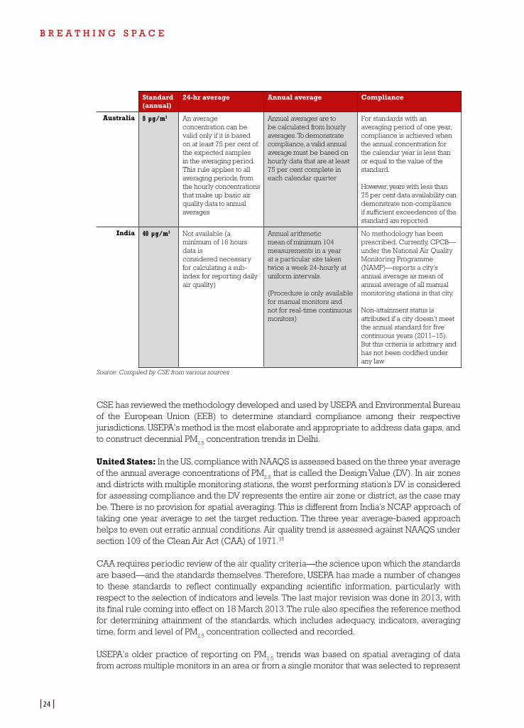
CSE has reviewed the methodology developed and used by USEPA and Environmental Bureau of the European Union (EEB) to determine standard compliance among their respective jurisdictions. USEPA's method is the most elaborate and appropriate to address data gaps, and to construct decennial PM
2.5 concentration trends in Delhi.
United States: In the US, compliance with NAAQS is assessed based on the three year average of the annual average concentrations of PM
2.5 that is called the Design Value (DV). In air zones
and districts with multiple monitoring stations, the worst performing station’s DV is considered for assessing compliance and the DV represents the entire air zone or district, as the case may be. There is no provision for spatial averaging. This is different from India’s NCAP approach of taking one year average to set the target reduction. The three year average-based approach helps to even out erratic annual conditions. Air quality trend is assessed against NAAQS under section 109 of the Clean Air Act (CAA) of 1971.35
CAA requires periodic review of the air quality criteria—the science upon which the standards are based—and the standards themselves. Therefore, USEPA has made a number of changes to these standards to reflect continually expanding scientific information, particularly with respect to the selection of indicators and levels. The last major revision was done in 2013, with its final rule coming into effect on 18 March 2013. The rule also specifies the reference method for determining attainment of the standards, which includes adequacy, indicators, averaging time, form and level of PM
2.5 concentration collected and recorded.
USEPA's older practice of reporting on PM2.5
trends was based on spatial averaging of data from across multiple monitors in an area or from a single monitor that was selected to represent
Standard (annual)
24-hr average Annual average Compliance
Australia 8 µg/m3 An average concentration can be valid only if it is based on at least 75 per cent of the expected samples in the averaging period. This rule applies to all averaging periods, from the hourly concentrations that make up basic air quality data to annual averages
Annual averages are to be calculated from hourly averages. To demonstrate compliance, a valid annual average must be based on hourly data that are at least 75 per cent complete in each calendar quarter
For standards with an averaging period of one year, compliance is achieved when the annual concentration for the calendar year is less than or equal to the value of the standard.
However, years with less than 75 per cent data availability can demonstrate non-compliance if sufficient exceedences of the standard are reported
India 40 µg/m3 Not available (a minimum of 16 hours data isconsidered necessary for calculating a sub- index for reporting daily air quality)
Annual arithmetic mean of minimum 104 measurements in a year at a particular site taken twice a week 24-hourly at uniform intervals.
(Procedure is only available for manual monitors and not for real-time continuous monitors)
No methodology has been prescribed. Currently, CPCB—under the National Air Quality Monitoring Programme (NAMP)—reports a city’s annual average as mean of annual average of all manual monitoring stations in that city.
Non-attainment status is attributed if a city doesn't meet the annual standard for five continuous years (2011–15). But this criteria is arbitrary and has not been codified under any law
Source: Compiled by CSE from various sources
B R E A T H I N G S P A C E
25
community-wide exposure. This method also did not include data substitution tests for data completeness.36 This approach was subsequently changed as it was recognized that the highest concentration in an area that also had disproportionately high impact on vulnerable communities in close proximity would lose focus under spatial averaging.37 This could lead to inequities in protection for at risk populations exposed to high PM
2.5 levels. These largely
included groups from lower socio-economic status, different age groups and minorities.
USEPA, therefore, concluded that spatial averaging may be inadequate to measure substantially greater exposure in some areas. From 2013, the spatial averaging method was discarded and new rules stated that ‘for an area with multiple monitors, the appropriate reporting monitor with the highest DV would determine the "attainment" status of that area.’38
Spatial averaging was, thus, considered an environment justice concern as poorer people are expected to live near roads, factories and other pollution source. This is even more relevant to India as high pollution areas in India are also more densely populated—and both high and low income groups are exposed to the harmful effects of the higher concentration of pollutants..
The big shift that, therefore, happened in 2013 in the US was the adoption of readings from the highest single worst-case monitor (rather than the average of all community area monitors). Subsequently, the compliance was based on the worst-case scenario. In fact, USEPA justifies this on the ground that monitoring in worst affected areas like roadsides does not make the standard more stringent but affords the intended protection.39 It is believed that if worst affected areas are averaged out with the lower concentration areas, public health cannot be adequately protected.
Canada: Canada's method of compliance with NAAQS is based on PM2.5
annual metric value, i.e., the three year average of the annual average concentrations. A PM
2.5 annual metric value is
calculated and considered valid if annual averages are available for at least two of the required three years. In cases where the metric value is based on only two years, the reported metric value for the station will be flagged appropriately.40 Canada has also revised its PM
2.5 NAAQS
from 10 µg/m3 to 8.8 µg/m3; the new limit came into effect in 2020.
European Union: EU has a different approach to establish trends. The Sixth Community Environment Action Programme adopted by Decision No 1600/2002/EC of the European Parliament and of the Council of 22 July 2002 establishes the need to reduce pollution to levels which minimize harmful effects on human health, paying particular attention to sensitive populations, and the environment as a whole, to improve the monitoring and assessment of air quality including the deposition of pollutants, and to provide information to the public.41
For standard compliance determination, the Average Exposure Indicator (AEI) is used, assessed as a three year running annual mean concentration averaged over all established sampling points. AEI, expressed in µg/m3, is based on measurements in urban background locations in zones and agglomerations throughout the territory of a member state.42 The key reference document is the DIRECTIVE 2008/50/EC of the European Parliament and of the Council (of 21 May 2008) on ambient air quality and cleaner air for Europe.
In order to ensure that information collected on air pollution is sufficiently representative and comparable across the community, standardized measurement techniques and common criteria for the number and location of measuring stations are used for the assessment of ambient air quality. The approach aims at a general reduction of concentrations in the urban background to ensure that large sections of the population benefit from improved air quality.
B R E A T H I N G S P A C E
26
For calculation of annual averages, 90 per cent of hourly values or (if not available) 24-hour values over the year are needed. The requirements for the calculation of annual mean do not include losses of data due to regular calibration or the normal maintenance of the instrumentation.
When assessing ambient air quality, the size of populations and ecosystems exposed to air pollution is taken into account. The territory of each member state is classified into zones or agglomerations reflecting population density. Wherever possible, modelling techniques are applied to enable point data to be interpreted in terms of geographical distribution of concentration. This serves as a basis for calculating the collective exposure of the population living in the area.43
Australia: In Australia, compliance is achieved when the annual concentration is less than or equal to the value of the standard. However, years with less than 75 per cent data availability can demonstrate non-compliance if sufficient excesses of the standard are reported.44
The global review also shows that compliance reporting does not necessarily depend on the number of stations. Even if there are a large number of stations, a few reference or primary monitors are identified based on certain criteria and are selected for data reporting. For instance, Beijing has one of the most dense monitoring grids in the developing world, with as many as 40 stations. But it bases annual average PM
2.5 reporting on 13 reliable stations
operating round-the-clock (see Box: China—nuanced analysis of contribution of action and meteorology to reduction in PM
2.5 related deaths). The average annual data from these stations
is used to report air quality trends.
Addressing issues of data availability United States: A 24-hour average concentration shall be considered valid if contains at least 75 per cent of the hourly averages (i.e., values of 18 hours) for the 24-hour period. 24-hour
ChinaNuanced analysis of contribution of action and meteorology to reduction in PM2.5 related deaths45
In China, dramatic reductions in PM2.5 concentration in the three key regions of Beijing–Tianjin–Hebei (BTH), Yangtze Delta (YRD) and the Pearl River Delta (PRD) between 2013 and 2017 have drawn considerable scientific attention. The annual PM2.5
concentration has been reduced from 106 μg/m3
to 64 μg/m3 in BTH, from 67 μg/m3 to 44μg/m3 in YRD, and from 47μg/m3 to34 μg/m3 in PRD. BTH has reduced the level by as much 40 per cent against the stated target of 25 per cent.
In a June 2019 independent study published in Environmental Health Perspective, a group of scientists have assessed the health benefits from this reduction and, more importantly, the relative contribution of different factors to the health
gain. More specifically, the study investigated the role of implementation of action plans to control emissions, changed meteorology, population growth and the change in baseline mortality rates to understand the contribution of action in relation to other factors.
The study found that the estimated total PM2.5 mortality in China was 1.389 million in 2013, which reduced substantially to 1.12 million in 2017. About 287,000 premature deaths were avoided annually between 2013 and 2017 due to implementation of action plans. Emissions control efforts have contributed 88.7 per cent of the total reduction while changes in meteorology and baseline mortality rates, and population growth have respectively contributed 9.6 per cent, 3.8 per cent, and -2.2 per cent to the total reduction in PM2.5 mortality. In BTH, the relative contribution of
B R E A T H I N G S P A C E
27
periods with seven or more missing hours shall also be considered valid if, after substituting zero for all missing hourly concentrations, the resulting 24-hour average daily value is greater than the level of the 24-hour PM
2.5 NAAQS (i.e. greater than or equal to 35.5 µg/m3).46
Annual average, on the other hand, is calculated as mean of the quarterly averages. A year meets data completeness requirements when data capture rates for all four quarters are at least 75 per cent. However, years with at least 11 creditable samples in each quarter shall also be considered valid if the resulting annual mean or resulting annual PM
2.5 NAAQS DV is greater
than the level of the applicable primary or secondary annual PM2.5
NAAQS.
In case one, two or three years do not meet the completeness requirements and, thus, would normally not be usable for the calculation of a valid annual PM
2.5 NAAQS DV, the annual PM
2.5
NAAQS DV shall nevertheless be considered valid if one of the substitution test conditions is met.
Canada: For continuous monitors, a daily 24-hour PM2.5
is to be considered valid if at least 75 per cent (18 hours) of the one-hour concentrations are available on the given day. If at least 18 hours are available, the denominator in the equation (for calculating the average value) will be the number of hours available. For manual samplers, the sampler must be operated for at least 18 hours in the day.47
Annual average is calculated as mean of the quarterly averages, if at least 75 per cent valid 24-hour PM
2.5 concentration data in the year is available, and at least 60 per cent valid 24-hour
PM2.5
concentration data in available for each quarter.
European Union: To calculate a valid 24-hour average, 75 per cent of the hourly averages (i.e., values of at least 18 hours) is needed. To calculate annual average, 90 per cent of the hourly values or (if not available) 24-hour values over the year are needed.48
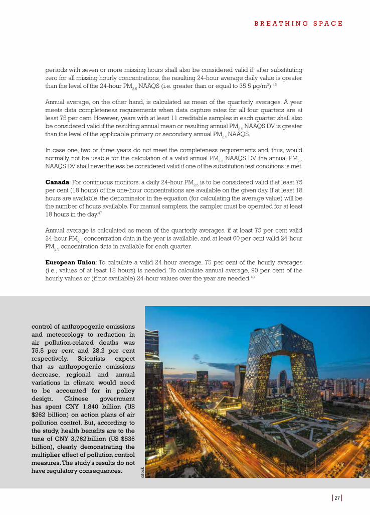
control of anthropogenic emissions and meteorology to reduction in air pollution-related deaths was 75.5 per cent and 28.2 per cent respectively. Scientists expect that as anthropogenic emissions decrease, regional and annual variations in climate would need to be accounted for in policy design. Chinese government has spent CNY 1,840 billion (US $262 billion) on action plans of air pollution control. But, according to the study, health benefits are to the tune of CNY 3,762 billion (US $536 billion), clearly demonstrating the multiplier effect of pollution control measures. The study's results do not have regulatory consequences.
iSto
ck
B R E A T H I N G S P A C E
28
The requirements for the calculation of annual mean do not include losses of data due to the regular calibration or the normal maintenance of instrumentation
Australia: An average concentration can be valid only if it is based on at least 75 per cent of the expected samples in the averaging period. This rule applies to all averaging periods, from the hourly concentrations that make up basic air quality data to annual averages.49
Annual averages are to be calculated from hourly averages. To demonstrate compliance, a valid annual average must be based on hourly data that is at least 75 per cent complete in each calendar quarter.
India: India has fixed criteria for assessing 24-hour averages and annual averages from manual monitors. A minimum of 16-hour data is considered necessary for estimating daily average or for calculating sub-index for reporting daily Air Quality Index.50
Currently, CPCB—under the National Air Quality Monitoring Programme (NAMP)—reports a city’s annual average as mean of annual average of all manual monitoring stations in that city. 'Non-attainment' status is attributed to a city if it doesn't meet the annual standard. To calculate annual averages, a minimum of 104 24-hour measurements in that year at a particular site taken twice a week at uniform intervals are needed.51
Other than this there is no other detailed methodology for reporting status of compliance in India. The current procedure for reporting annual average is only available for manual monitors and not for real-time continuous monitors.
Addressing issues of data completenessAll air quality regulators face the challenge of missing data and data gaps—more so in India. This happens due to technical glitches, operational issues, equipment failure, accidents and other reasons, but it is not a problem that can't be addressed. Globally, air quality regulators have developed methods for minimum data requirements for estimating daily 24-hour averages as well as annual averages. Many countries also have regulations that require a proper data substitution and completeness method.
United States: USEPA has the most elaborate rules on addressing data gaps and for data completeness. According to these rules, three year valid annual means are required to produce a valid annual PM
2.5 DV to compare with US NAAQS. A year is considered to have met its data
completeness requirement if the ‘quarterly data capture rates for all the four quarters are at least 75 per cent’ of the schedule monitoring.
Therefore, in the case of manual monitors, as the minimum requirement is data for every sixth day, at least 11 creditable samples in each quarter in a year are considered valid if the resulting annual mean or resulting annual PM
2.5 DV is greater than the level of applicable annual PM
standard.52
What happens if there are years or quarters in a year when this minimum requirement of 75 per cent data in a year is not met either by manual or real-time monitors (which can be 11 minimum samples for manual monitors)? For that, USEPA has laid down detailed rules for data substitution tests to the effect that the three year annual DV for PM
2.5 concentration shall still be
considered valid if it passes one or two data substitution tests as stipulated in the rules.53
In case one, two or three years (in the three year average rule for PM2.5
DV) do not meet data completeness requirements and, thus, would normally not be usable for the calculation of a
B R E A T H I N G S P A C E
29
valid annual PM2.5
DV. The annual PM2.5
NAAQS DV shall be considered valid if one of the test conditions specified is followed. These rules have been codified to show how data substitution is possible to construct a trend (see Box: What are the rules for data completeness?)
There are instances in the US where the annual trend has been constructed for sites even when the monitor has not been functioning and there is no annual data. For example, an interesting method was devised to deal with missing data at a station in San Joaquin Valley, California. The station had been burned down in an electric fire.54 In its final report of 2019, USEPA retained the valley as 'non-attainment' based on DV of the burned down station. It noted, ‘San Joaquin Valley‘s 2013–15, 2014–16, and 2015–17 DV site (Corcoran-Patterson) does not have data from 7 February 2015 to 31 December 2015 due to a fire that destroyed the site. Based on DV calculation methodologies described in 40 CFR Part 50, Appendix N, the DV for Corcoran-Patterson is considered valid despite the missing 2015 data.’55
Filling the gap from collocated monitors: There is another important method of leveraging data from collocated monitors. Collocation means two or more monitors being adjacent and operating simultaneously, ‘separated by a distance that is large enough to preclude the air sampled by any of the monitors affected by any of the devices, but small enough so that all devices obtain identical or uniform ambient air samples that are equally representative of the general area in which they are located. One monitor is designated as primary and others are collocated. It is implicit that all are deemed suitable for applicable NAAQS comparison.’56
The combined site dataset represents data for primary monitors augmented with data from collocated monitors. This logic is applied at the site level. According to USEPA rules, if the primary monitor does not produce valid value for a particular day, but a value is available from the collocated monitor, then that collocated value can be considered as part of the combined site data record. If more than one collocated daily value is available, the average of those valid collocated values shall be used as the daily value. The data record resulting from this procedure is referred to as the 'combined site data record.'57
USEPA has clear criteria of assessing how different monitors are correlated with each other. Under its Ambient Air Monitoring Network Assessment Guidance, monitors with values that correlate well (higher than 75 per cent) with values from another monitor may be redundant. The idea of a monitoring network is to keep track of the changes in air quality, both temporally and spatially. Ideally, the network needs to have one or two urban background monitors installed based on topography and area, and the rest of the network needs to be optimized to limit itself to monitors that exhibit unique temporal concentration variations relative to other monitors that are likely to be important for assessing local emissions, transport and spatial coverage. This approach has helped reduce the number of monitoring stations and resources needed to operate and maintain them.58
If USEPA criteria of collocation are applied to Delhi then, on an average, Delhi’s 38 monitoring stations are 77 per cent correlated. The enhanced data, therefore, becomes more robust and representative of all sites.
Also, if over a period of time air pollution is brought under control and the trends of different pollutants stabilizes and declines, as has happened in the US and several parts of Europe, the number of monitors can also be curtailed.
Monitoring airshedsThe monitoring of larger airsheds is yet another issue that will have to be addressed within the legal monitoring framework in India. The science of air pollution has clearly established that air
B R E A T H I N G S P A C E
30
quality management requires an airshed- or regional-level approach for effective mitigation. Other countries have adopted similar approaches for integrated airshed- or air basin-based monitoring.
In China, air pollution control action in Beijing required an integrated monitoring and reporting approach across seven provinces and 63 cities for regional-level reduction in PM
2.5 levels.60
In the US, the geographical unit used for compliance is metropolitan statistical areas (MSAs), Indian equivalent of which will be an urban agglomeration. For instance, New York–Newark–Jersey City is the biggest MSA in the US with a population of 20.3 million people, according to the 2017 Census.61 This means a single (worst) station’s or site's reading determines the air quality level of the whole MSA, even though it has over 30 monitoring stations.
Cities are not the core geography for monitoring in the US and enforcing air quality standards. The country generally relies on air basins as areas for establishing compliance with national standards. For instance, California is divided into 15 air basins to better manage air pollution. Air basin boundaries are determined by grouping together areas with similar geographical and meteorological features. Political boundaries are also considered in determining these boundaries.62 Some air basins are relatively small, while others are quite large. Some are very much like a basin, consisting of valleys surrounded by mountains, while others are more
What are the rules of data completeness?59
Key highlights of some of the USEPA rules are as follows:(i) An annual PM2.5 standard design value (DV) that is above the level of NAAQS can be validated if it passes the minimum quarterly value data substitution test. This type of data substitution is permitted only if there are at least 30 days across the three quarters of the three years under consideration (e.g., collectively, quarter 1 of year 1, year 2 and year 3) from which quarter-specific low value can be selected. Data substitution will be performed in all quarters that have less than 11 creditable samples.
To do this, USEPA identifies, for each quarter that is deficient in data (with less than 11 creditable samples), the lowest reported daily value for that quarter looking across those three months of all three years under consideration. If after substituting the missing values in this manner with the lowest reported daily value for a quarter daily value in matching deficient
quarters leads to a recalculated annual PM2.5 DV that is greater than the PM2.5 standard, then it is deemed to have passed the diagnostic test and is valid, and the PM2.5 NAAQS is deemed to have been violated in that three year period.
(i) An annual PM2.5 NAAQS DV that is equal to or below the level of the NAAQS can be validated if it passes the maximum quarterly value data substitution test. This type of data substitution is permitted only if there is at least 50 per cent data capture in each quarter that is deficient of 75 per cent data capture in each of the three years under consideration. Data substitution will be performed in all quarters that have less than 75 per cent data capture but at least 50 per cent data capture.
If any quarter has less than 50 per cent data capture, this substitution test cannot be used. In such a case, USEPA identifies for each deficient quarter (those with less than 75 per cent but at least 50 per cent data capture) the highest reported daily value for that quarter, excluding state-flagged data affected by exceptional events which have been approved by USEPA's Administrator for exclusion, looking across
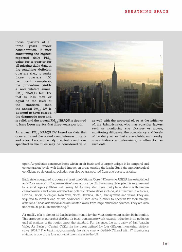
B R E A T H I N G S P A C E
31
open. Air pollution can move freely within an air basin and is largely unique in its temporal and concentration levels with limited impact on areas outside the basin. But if the meteorological conditions so determine, pollution can also be transported from one basin to another.
Each state is required to operate at least one National Core (NCore) site. USEPA has established an NCore network of 'representative' sites across the US. States may delegate this requirement to a local agency. States with many MSAs may also have multiple airsheds with unique characteristics and, often, elevated air pollution. These states include, at a minimum, California, Florida, Illinois, Michigan, New York, North Carolina, Ohio, Pennsylvania and Texas. They are required to identify one or two additional NCore sites in order to account for their unique situations. These additional sites are located away from large emissions sources. They are also under multi-pollutant monitoring.63
Air quality of a region or air basin is determined by the worst performing station in the region. This approach ensures that all of the air basin continues to work towards reduction in air pollution until all stations in the region meet the standard. For instance, the air quality of San Joaquin Valley Air Basin in Central California has been defined by four different monitoring stations since 2009.64 The basin, approximately the same size as Delhi–NCR and with 17 monitoring stations, is one of the four non-attainment areas in the US.
those quarters of all three years under consideration. If after substituting the highest reported daily PM2.5 value for a quarter for all missing daily data in the matching deficient quarters (i.e., to make those quarters 100 per cent complete), the procedure yields a recalculated annual PM2.5 NAAQS test DV that is less than or equal to the level of the standard, then the annual PM2.5 DV is deemed to have passed the diagnostic tests and is valid, and the annual PM2.5 NAAQS is deemed to have been met for that three years period.
An annual PM2.5 NAAQS DV based on data that does not meet the stated completeness criteria and also does not satisfy the test conditions specified in the rules may be considered valid
as well with the approval of, or at the initiative of, the Administrator, who may consider factors such as monitoring site closures or moves, monitoring diligence, the consistency and levels of the daily values that are available, and nearby concentrations in determining whether to use such data.
iSto
ck
B R E A T H I N G S P A C E
32
CSE's global review has established that monitoring rules in India will have to be made more explicit to better define methods for data completeness, adoption of averaging systems for trend reporting, representation of area-wide air quality, leveraging of real-time monitoring for air quality trend reporting, even while making efforts to improve data quality.
To build this case further, a detailed analysis of long-term trends in Delhi’s air quality have been carried in the context of the global methods.
THE WAY FORWARD
This assessment by CSE, carried out in the backdrop of clean air action in the city, has yielded many lessons that will be useful for other cities and in national-level interventions. The clear message is that air quality trend will have to be tracked diligently and methodically to determine compliance with the overall reduction target set under NCAP for 2024 and in meeting NAAQS. Air quality scientists must revisit the adequacy of the practice of using data from only manual monitors to report annual averaged for trend reporting. As the real-time monitoring network of India expands alongside the manual monitoring grid, cities will need methods to analyze the voluminous data generated therefrom. Such methods must take stock of data completeness and address issues of data gaps and data availability. CSE’s global review shows that several such approaches (vis-à-vis completeness) have been codified in different countries.
In the current analysis, CSE has made use of USEPA method to analyze air quality trends in Delhi while considering the unique issues related to data gaps and availability. It has taken into account the fact that while the application of the method is correct, this analysis needs a few caveats related to the fact that most of the thresholds have been developed in the context of data infrastructure of the US. These thresholds may change once India develops its own method. But the results certainly show indicative quantifiable changes in Delhi’s air quality. The technical and governance aspects of NCAP will have to be strengthened to allow such reporting.
This is where the role of CPCB becomes crucial. The board needs to define these methods in detail to enable SPCBs to assess long-term air quality trends in their respective states and zones to report change as well as targets for the next level of reduction. This exercise should be matched by stronger intervention for quality control of air quality data—both real-time and manual.
However, we must also realize that this intervention to develop a method for more inclusive and robust reporting of air pollution and action is only a part of a range of reforms that NCAP requires to strengthen the sector's governance framework and compliance regime. Bigger legal reforms are needed to make clean air action plans legally enforceable. However, that discussion is beyond the immediate scope of this specific study.
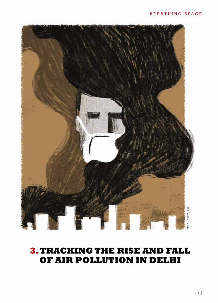
B R E A T H I N G S P A C E
33
3. TRACKING THE RISE AND FALL OF AIR POLLUTION IN DELHI
TARI
QU
E A
ZIZ
/ C
SE
B R E A T H I N G S P A C E
34
3(A). DECODING DELHI’S AIR QUALITY TRENDS
How has Delhi’s air quality changed over time? The past decade has been witness to an intense battle for clean air. Several multi-sectoral measures have been initiated. At the turn of the new decade, it is important to track annual and seasonal trends in particulate pollution and assess the status of compliance with respect to PM
2.5 standards. This will help us chart a new roadmap.
Delhi is already under intense monitoring scrutiny for implementation of its two action plans for air pollution reduction—the Comprehensive Action Plan and the Graded Response Action Plan (GRAP). Target setting for air pollution reduction requires understanding of the shifts over time.
Air quality analysis of Delhi demonstrates application of some of the global methods for trend and compliance analysis and the approaches to data completeness to get more reliable indicative trends. CPCB has continued to report annual average data based solely on manual monitors, with serious concerns around quality of data and minimum data requirement. Data available from the CPCB website shows that several manual monitors have not met the minimum data requirement of 104 days of monitoring in recent years. Delhi has six PM
2.5 manual monitors.
On an average, data of 62 days in 2015, 74 days in 2016, 67 days in 2017, and 60 days in 2018 is available.65 There is no information on how well distributed this data is across the year for it to be adequately representative.
In the meantime, there has been substantial expansion in real-time air quality monitoring. The number of real-time monitors has increased from one in 2010–11 to 38 in 2020; 70, if we consider the larger region. Data from real-time monitors is publicly available. Currently, this dataset is being used to report daily air quality based on the National Air Quality Index. The reporting comes with a rider to the effect that, 'For Delhi–NCR (with multiple monitoring locations), average value is used to indicate air quality. Air quality may show variations across locations, and averaging is not a scientifically sound approach. However, for the sake of simplicity this method is being used.'66 This rider cannot operate in the new paradigm, where reporting is needed under NCAP, and will have to be addressed.
CSE analyzed PM2.5
concentration in Delhi to figure out city-wide temporal trends and to establish whether we can discern changing patterns in the distribution of days with varying intensity of pollution across locations; and if it is possible to see more localized hotspots. Trends in air pollution are affected by emission of pollutants, action against pollution and meteorological factors. Meteorology events influence short-term and seasonal trends that also have a bearing on long-term trends. In the long run, the overall trend indicates more certainty in change due to action. It is possible to construct indicative long-term historical trends to know the shifts in the nature of the problem. Governments will have to look at the monitored data and understand the trend to refine their action plans.
DELHI’S AIR QUALITY DATABASE
The air quality data used in this analysis has been obtained from CPCB’s online portal Central Control Room for Air Quality Management—All India for the period 2010–19.
Granularity of the data is 15-minute average concentration of PM2.5
. This data was downloaded by CSE in two lots; data upto end of 2018 in August 2019 and data for 2019 in January 2020.
B R E A T H I N G S P A C E
35
The data is for all 38 real-time monitoring stations in the National Capital Territory of Delhi. Data reporting on CPCB’s online portal has been added as new stations have been added over time. Anyone can access this data from https://app.cpcbccr.com/ccr/#/ caaqm-dashboard-all/caaqm-landing/data as the database is publicly available.
Of the 38 stations, seven are operated by Indian Metrological Department (IMD), seven by CPCB and 24 by DPCC. East Arjun Nagar station, manned by CPCB, has no data entry for the entire study period. At least four real-time stations have data entries since 2011 and six since 2012. Data from all these stations has been reported on the CPCB website.
The raw dataset has over 3.38 million data points. They are non-uniformly distributed among the 38 stations and over many years. As Delhi has continuously expanded its monitoring grid, the number of stations working each year is increasing; 2010 had one working station and 2019 had 37 working stations (see Graph 1: Timeline of and data availability at air quality stations in Delhi). This has led to observed non- uniformity in spatial and temporal distribution of data in the given dataset.
The raw dataset has been cleaned for outliers and erroneous entries—very high or very low values have been rechecked with the collocated database. The dataset has also been checked for default entries like 999, and 985 that are at times used as filler for missing data entries. All such erroneous entries have been removed. The dataset was further screened for flat lines, indicating technical snags in the reporting of the data at each station. Data points corresponding to these flat lines were also removed from the dataset.
The final cleaned dataset has about 3.19 million data points. As data is available for 15-minutes averages, which is a regulatory requirement, hourly averages have been computed based on that. For each station, data availability was computed at the quarterly level. It was deemed critical to establish data availability for each quarter or season instead of just the annual level.
To assess data gaps and data completeness, USEPA criteria and rules have been applied to make the vast dataset usable for constructing a reliable long-term trend and assess status of compliance.67
Addressing data gapsThis analysis has assessed data gaps for each quarter of every year since 2011 for all stations. The nature of data gaps varies across stations and over time. To assess the data gaps, USEPA criteria of minimum 75 per cent has been considered. Analysis of station-wise data gaps each year shows that there are quarters, especially in the earlier part of the decade, when data availability requirement is less than 75 per cent. This improves with time and with newer stations.
Even with data gaps, the overall data availability from real-time stations is much better than the manual stations. Manual data can represents air quality of 28.5 per cent days in a year. If examined from the perspective of sample requirements for manual stations (104 days in a year or 26 days in a quarter) to assess legal compliance with NAAQS, then 436 quarters of the cumulative 556 quarters, or 79 per cent of all quarters with real-time data, meet the data completeness requirement.
The oldest five stations—IHBAS, ITO, Mandir Marg, Punjabi Bagh and RK Puram—for which real-time data is comparatively continuously available (since 2012), have been considered for long-term trend analysis. Data gaps are bigger for earlier years. Application of the criteria of 75 per cent availability to these five stations shows that at least 83 quarters of the 160 quarters
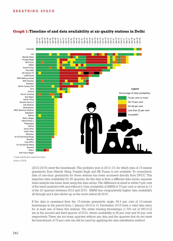
B R E A T H I N G S P A C E
36
(2012-2019) meet the benchmark. The problem year is 2014–15, for which data of 15-minute granularity from Mandir Marg, Punjabi Bagh and RK Puram is not available. To crosscheck, data of one-hour granularity for these stations has been accessed directly from DPCC. This improves data availability for 95 quarters. As this data is from a different data series, separate trend analysis has been done using this data series. The difference in result is within 5 per cent of the trend analyzed with and without it. Data availability at IHBAS is 75 per cent or above in 13 of the 20 quarters between 2012 and 2016. IHBAS has comparatively higher data availability all through and it also shows up as the worst station till 2016.
If the data is examined from the 15-minute granularity angle, 99.4 per cent of 15-minute timestamps in the period from 1 January 2012 to 31 December 2019 have a valid data entry for at least one of these five stations. The entire missing timestamps (1,728 out of 280,512) are in the second and third quarter of 2012, where availability is 89 per cent and 90 per cent respectively. There are not many quarters without any data and the quarters that do not meet the benchmark of 75 per cent can still be used by applying the data substitution method.
Citywide
ITOMandir MargPunjabi Bagh
RK PuramIHBAS
Anand ViharPusa IMD
IGI Airport T3Lodhi Road
CRRI Mathura RoadNSIT Dwarka
ShadipurNorth Campus DU
DTUSirifort
Burari CrossingAya Nagar
Ashok ViharDwarka Sector 8
JLN StadiumJahangirpuri
MDC National StadiumNajafgarh
NarelaNehru Nagar
Okhla Phase 2Patparganj
RohiniSonia ViharVivek Vihar
WazirpurDr KS Shooting Range
MundkaPusa DPCC
Sri Aurobindo MargBawana
AlipurEast Arjun Nagar
Oct
-19
Jul-
19
Ap
r-19
Ja
n-1
9 O
ct-1
8 Ju
l-18
A
pr-
18
Jan
-18
Oct
-17
Jul-
17
Ap
r-17
Ja
n-1
7 O
ct-1
6 Ju
l-16
A
pr-
16
Jan
-16
Oct
-15
Jul-
15
Ap
r-15
Ja
n-1
5 O
ct-1
4 Ju
l-14
A
pr-
14
Jan
-14
Oct
-13
Jul-
13
Ap
r-13
Ja
n-1
3 O
ct-1
2 Ju
l-12
A
pr-
12
Jan
-12
Oct
-11
Jul-
11
Ap
r-11
Ja
n-1
1 O
ct-1
0 Ju
l-10
A
pr-
10
Jan
-10
Graph 1: Timeline of and data availability at air quality stations in Delhi
* Data substitution cannot be done.
Source: CPCB
Legend
Percentage of data availability
75 per cent or more
50–75 per cent
25–50 per cent
Less than 25 per cent
Unusable*
B R E A T H I N G S P A C E
37
Overall, data availability is very good for 2018 and 2019, with only 12 quarters having less than 75 per cent data availability, and just one quarter having less than 26 days of data availability, out of the cumulative 284 quarters. Overall, 213 of the 556 quarters (2012–19) or 38 per cent of all quarters, have data availability of less than 75 per cent. These quarters required data substitution tests.
Data of the five stations on the basis of which trends have been established correlates better, in the range of 0.6 and 0.81. ITO and Mandir Marg have the highest correlation (0.81) while IHBAS and Punjabi Bagh are the least correlated stations (at 0.60). The distance between these station pairs can be used to explain the difference in the correlation coefficient. But these variations are not high enough to establish presence of unique atmospheric chemistry within the city of Delhi. While this will have to be assessed further, it seems quite likely that these variations can be attributed to pollution from nearby sources instead of to variations in the wider ambient air of the area. Correlation numbers are even higher for newer stations. For instance, JNL Stadium, National Stadium, Okhla Phase 2 and Sri Aurobindo Marg have correlation coefficients of 0.9 or higher among themselves. USEPA generally applies a collocation factor and considers station pairs with correlation coefficient higher than 0.75 as collocated and treats data from the station with lower annual average as redundant.
Addressing issues of data completenessThe immediate question was: Is there a way to address the data gap in PM
2.5 concentration to
get a reasonable indication of the trend and status of compliance?
In search for an answer, this study has referred to the USEPA method as given in US Code of Federal Regulations. These documents have laid out method of analysis, data substitution tests and how to address missing or inadequate data to create a trend. To overcome the limitation of data gaps, especially for the earlier year in the decade, the USEPA method of data completeness has been applied to the vast data points generated over the years in Delhi.
Hourly-averages were constructed from the 15-minute averages available from CPCB. 24-hour averages have been computed using hourly data—given that 75 per cent or 18 hours of data is available for each such day. In case this requirement is not met, USEPA's substitution method has been used for validating the 24-hour average.
Annual averages were calculated as a mean of quarterly averages, which are computed using valid 24-hour averages. DV for all stations for the entire study period was calculated as the average of three years. The validity of the DV was determined by establishing the availability of 75 per cent of 24-hour averages for all quarters in the three years period. In case the data availability for a quarter was less than 75 per cent, a minimum quarterly value data substitution test (as per the USEPA method) was conducted. This method can only be applied if, cumulatively, at least 30 days of valid data is available for that quarter (say the third quarter of a year) over the course of the three years. If the criterion is met, all missing data in that quarter for all three years is replaced with the minimum recorded 24-hour average among the available data. If the resultant DV, after this replacement, is above the annual NAAQS then that DV (without the replacements) is considered valid. If the criterion is not met, then the DV is declared invalid.
Overall, of the 38 current stations, the five oldest stations were found to have valid DVs for the entire study period. Fifteen stations were found to have at least one valid DV (see Table 2: Station-wise trends in design values). Only those stations where data substitution tests have not been possible for some parts of the year due to paucity of data have been rejected (marked in red in the table).
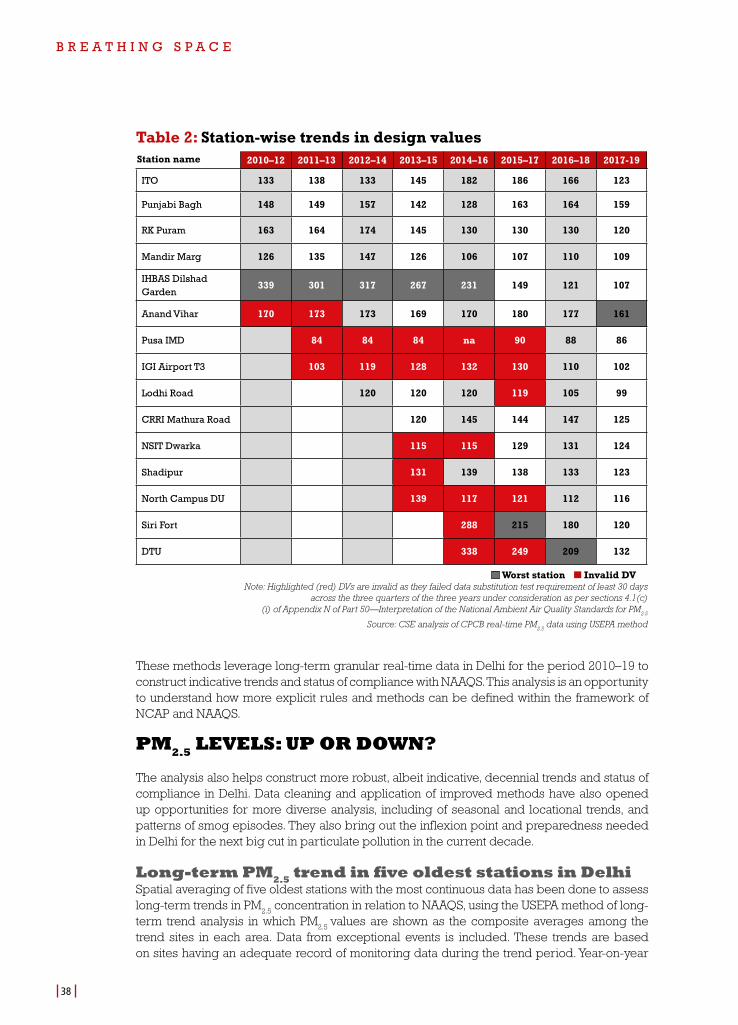
B R E A T H I N G S P A C E
38
These methods leverage long-term granular real-time data in Delhi for the period 2010–19 to construct indicative trends and status of compliance with NAAQS. This analysis is an opportunity to understand how more explicit rules and methods can be defined within the framework of NCAP and NAAQS.
PM2.5 LEVELS: UP OR DOWN?
The analysis also helps construct more robust, albeit indicative, decennial trends and status of compliance in Delhi. Data cleaning and application of improved methods have also opened up opportunities for more diverse analysis, including of seasonal and locational trends, and patterns of smog episodes. They also bring out the inflexion point and preparedness needed in Delhi for the next big cut in particulate pollution in the current decade.
Long-term PM2.5 trend in five oldest stations in DelhiSpatial averaging of five oldest stations with the most continuous data has been done to assess long-term trends in PM
2.5 concentration in relation to NAAQS, using the USEPA method of long-
term trend analysis in which PM2.5
values are shown as the composite averages among the trend sites in each area. Data from exceptional events is included. These trends are based on sites having an adequate record of monitoring data during the trend period. Year-on-year
ITO 133 138 133 145 182 186 166 123
Punjabi Bagh 148 149 157 142 128 163 164 159
RK Puram 163 164 174 145 130 130 130 120
Mandir Marg 126 135 147 126 106 107 110 109
IHBAS Dilshad Garden
339 301 317 267 231 149 121 107
Anand Vihar 170 173 173 169 170 180 177 161
Pusa IMD 84 84 84 na 90 88 86
IGI Airport T3 103 119 128 132 130 110 102
Lodhi Road 120 120 120 119 105 99
CRRI Mathura Road 120 145 144 147 125
NSIT Dwarka 115 115 129 131 124
Shadipur 131 139 138 133 123
North Campus DU 139 117 121 112 116
Siri Fort 288 215 180 120
DTU 338 249 209 132
Note: Highlighted (red) DVs are invalid as they failed data substitution test requirement of least 30 days across the three quarters of the three years under consideration as per sections 4.1(c)
(i) of Appendix N of Part 50—Interpretation of the National Ambient Air Quality Standards for PM2.5
Source: CSE analysis of CPCB real-time PM2.5
data using USEPA method
Table 2: Station-wise trends in design values2010–12 2011–13 2012–14 2013–15 2014–16 2015–17 2016–18 2017-19Station name
Worst station Invalid DV
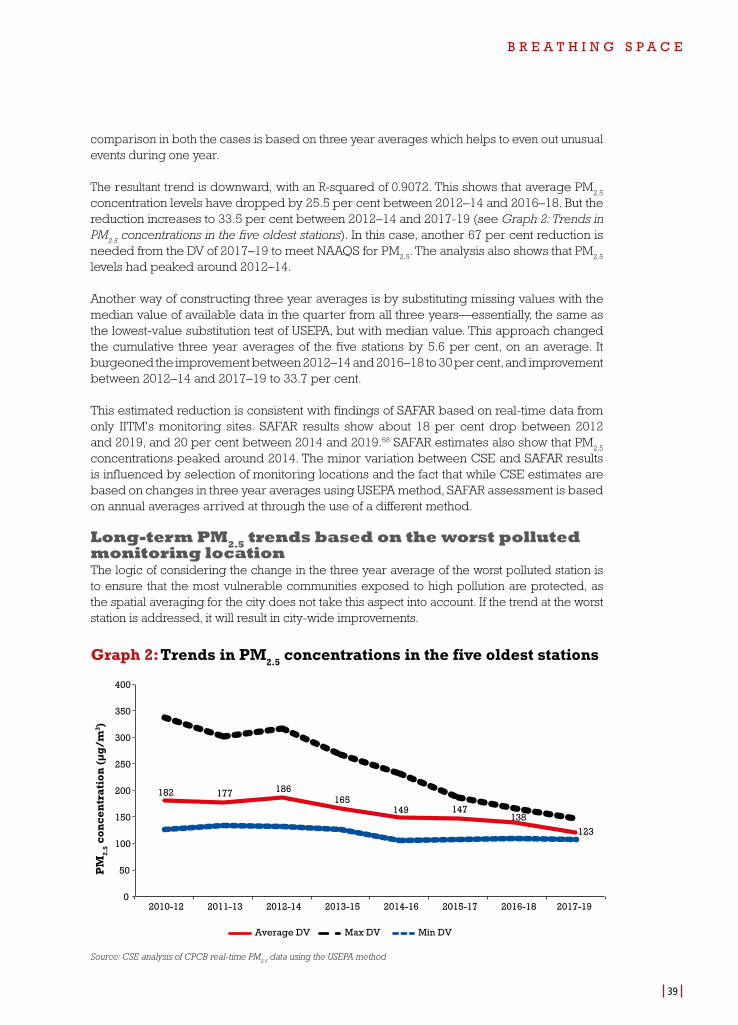
B R E A T H I N G S P A C E
39
comparison in both the cases is based on three year averages which helps to even out unusual events during one year.
The resultant trend is downward, with an R-squared of 0.9072. This shows that average PM2.5
concentration levels have dropped by 25.5 per cent between 2012–14 and 2016–18. But the reduction increases to 33.5 per cent between 2012–14 and 2017-19 (see Graph 2: Trends in PM
2.5 concentrations in the five oldest stations). In this case, another 67 per cent reduction is
needed from the DV of 2017–19 to meet NAAQS for PM2.5
. The analysis also shows that PM2.5
levels had peaked around 2012–14.
Another way of constructing three year averages is by substituting missing values with the median value of available data in the quarter from all three years—essentially, the same as the lowest-value substitution test of USEPA, but with median value. This approach changed the cumulative three year averages of the five stations by 5.6 per cent, on an average. It burgeoned the improvement between 2012–14 and 2016–18 to 30 per cent, and improvement between 2012–14 and 2017–19 to 33.7 per cent.
This estimated reduction is consistent with findings of SAFAR based on real-time data from only IITM's monitoring sites. SAFAR results show about 18 per cent drop between 2012 and 2019, and 20 per cent between 2014 and 2019.68 SAFAR estimates also show that PM
2.5
concentrations peaked around 2014. The minor variation between CSE and SAFAR results is influenced by selection of monitoring locations and the fact that while CSE estimates are based on changes in three year averages using USEPA method, SAFAR assessment is based on annual averages arrived at through the use of a different method.
Long-term PM2.5 trends based on the worst polluted monitoring locationThe logic of considering the change in the three year average of the worst polluted station is to ensure that the most vulnerable communities exposed to high pollution are protected, as the spatial averaging for the city does not take this aspect into account. If the trend at the worst station is addressed, it will result in city-wide improvements.
Graph 2: Trends in PM2.5 concentrations in the five oldest stations
182 177 186 165
149 147 138
123
0
50
100
150
200
250
300
350
400
2010-12 2011-13 2012-14 2013-15 2014-16 2015-17 2016-18 2017-19
PM
2.5 c
once
ntr
atio
n (µ
g/m
3 )
Average DV Max DV Min DV
Source: CSE analysis of CPCB real-time PM2.5
data using the USEPA method
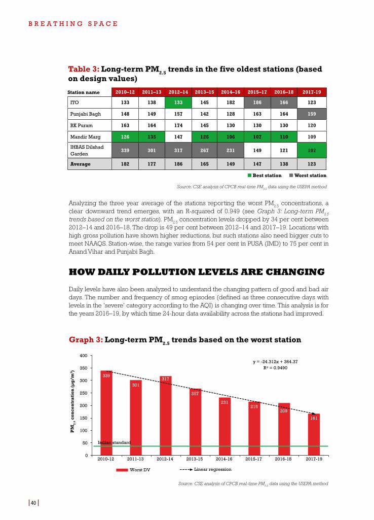
B R E A T H I N G S P A C E
40
Analyzing the three year average of the stations reporting the worst PM2.5
concentrations, a clear downward trend emerges, with an R-squared of 0.949 (see Graph 3: Long-term PM
2.5
trends based on the worst station). PM2.5
concentration levels dropped by 34 per cent between 2012–14 and 2016–18. The drop is 49 per cent between 2012–14 and 2017–19. Locations with high gross pollution have shown higher reductions, but such stations also need bigger cuts to meet NAAQS. Station-wise, the range varies from 54 per cent in PUSA (IMD) to 75 per cent in Anand Vihar and Punjabi Bagh.
HOW DAILY POLLUTION LEVELS ARE CHANGING
Daily levels have also been analyzed to understand the changing pattern of good and bad air days. The number and frequency of smog episodes (defined as three consecutive days with levels in the 'severe' category according to the AQI) is changing over time. This analysis is for the years 2016–19, by which time 24-hour data availability across the stations had improved.
2010–12 2011–13 2012–14 2013–15 2014–16 2015–17 2016–18 2017-19
Table 3: Long-term PM2.5 trends in the five oldest stations (based on design values)
Station name
ITO 133 138 133 145 182 186 166 123
Punjabi Bagh 148 149 157 142 128 163 164 159
RK Puram 163 164 174 145 130 130 130 120
Mandir Marg 126 135 147 126 106 107 110 109
IHBAS Dilshad Garden
339 301 317 267 231 149 121 107
Average 182 177 186 165 149 147 138 123
Source: CSE analysis of CPCB real-time PM2.5
data using the USEPA method
Best station Worst station
Graph 3: Long-term PM2.5 trends based on the worst station
Source: CSE analysis of CPCB real-time PM2.5
data using the USEPA method
339
301 317
267
231 215
209
161
y = -24.312x + 364.37 R = 0.9490
0
50
100
150
200
250
300
350
400
2010-12 2011-13 2012-14 2013-15 2014-16 2015-17 2016-18 2017-19
PM
2.5 c
once
ntr
atio
n (µ
g/m
3 )
Worst DV Linear regression
Indian standard
B R E A T H I N G S P A C E
41
USEPA method and the Indian databaseAs no official method exists in India regarding data substitution and data completeness to address data gaps or detailed codified rules for assessment of long-term trends in concentration and for compliance with NAAQS, this study has applied detailed methods of USEPA. To ensure accuracy of application of these methods and the appropriateness of their application to the Indian data base, CSE consulted with air pollution scientists of USEPA.
Application of the USEPA method to Delhi's database is technically and statistically accurate. But given the fact that the USEPA method has been developed in the context of air quality monitoring conditions and infrastructure present in the US, its application in India needs to be considered with a few caveats.
First of all, when India develops its own method for data completeness, it may change some of the threshold requirements for data availability and completeness. That may have a bearing on results. Given that the sampling requirement in the US is once every six days, technically 12 samples or 12 days of data in a quarter also meet the 75 per cent data completeness threshold. Due to stronger quality assurance and control in the US, actual data availability is of a higher order. On the other hand, since continuous monitors record data everyday, lower data completeness threshold might still be valid.
The second caveat is that in places with large temporal variability (as is the case in India), more valid samples may be needed per quarter in order to characterize the mean with low uncertainty. A statistical test on the locations with more complete datasets is needed to establish exactly what the threshold should be for India.
Another caveat is regarding missing data. USEPA has detailed protocols and methodologies to overcome data gaps and address issues with data completeness when the NAAQS threshold is not met. Missing data can be substituted by the lowest quarterly value (from the preceding or succeeding two years), to test if the three year average of a station exceeds NAAQS, or substituted by the highest quarterly value, to test if the design value (three year average) is below NAAQS. This replacement is to test compliance in reference to the standard, and the average values arrived at after replacement are termed as the test design value, while the official average of that station remains the one arrived at without replacement. This is because both tests either systematically overestimate or underestimate pollution levels. For official average, the original average without replacement (but validated by the substitution test) is used. If the missing data is considerably higher then other replacement strategies like mean or median of available valid data can be used to establish the official number.
The methodology for data substitution in the 40 CFR Part 50 of USEPA also works for large data gaps spanning over multiple quarters. In such cases, data from two consecutive years is used to carry out the substitution test. It was recently done for the Corcoran air monitoring station in the San Joaquin valley district of California. The Corcoran station was destroyed in February 2015 and the new monitor could only be installed in the fall of 2016. USEPA used three year average calculation methodology described in 40 CFR Part 50 and found that the DV for Corcoran station was valid despite the missing 2015 data.
Another caveat is regarding the selection of stations to be representative of a region or city. USEPA has identified certain stations to be long-term primary station. These stations are designed to represent average conditions across the area, rather than pollution from nearby sources. It also ensures minimal overlap among the area being represented by each long-term trend stations. In India, there is a clearly defined protocol for location of monitoring stations, but no long-term primary stations.
Source: Personal communication with Robert Pinder, USEPA, 17 December 2019
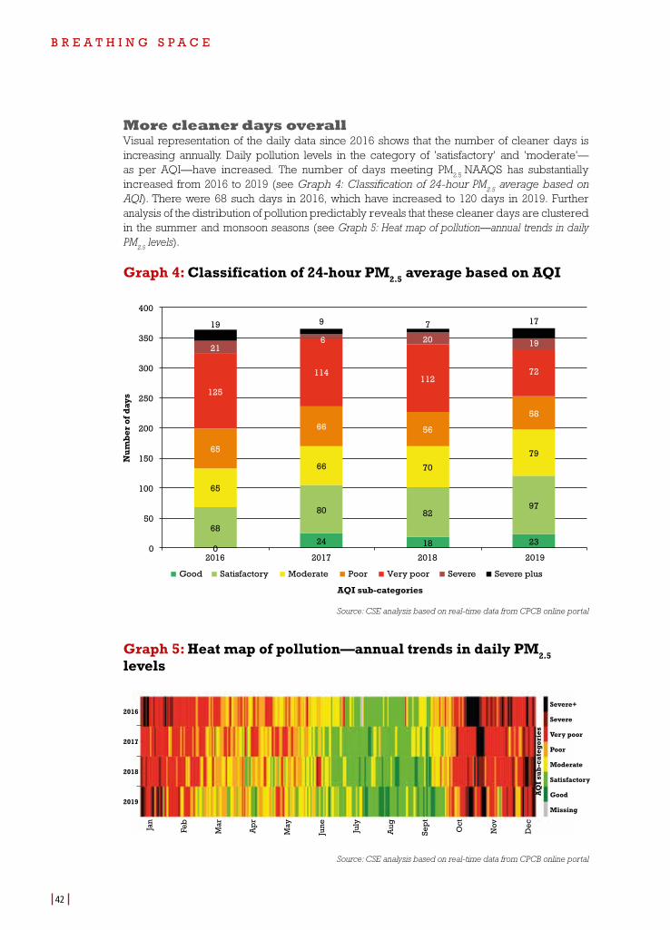
B R E A T H I N G S P A C E
42
More cleaner days overallVisual representation of the daily data since 2016 shows that the number of cleaner days is increasing annually. Daily pollution levels in the category of 'satisfactory' and 'moderate'—as per AQI—have increased. The number of days meeting PM
2.5 NAAQS has substantially
increased from 2016 to 2019 (see Graph 4: Classification of 24-hour PM2.5
average based on AQI). There were 68 such days in 2016, which have increased to 120 days in 2019. Further analysis of the distribution of pollution predictably reveals that these cleaner days are clustered in the summer and monsoon seasons (see Graph 5: Heat map of pollution—annual trends in daily PM
2.5 levels).
Graph 4: Classification of 24-hour PM2.5 average based on AQI
0 24 18 23
68
80 82 97
65
66 70
79 65
66 56
58
125
114 112
72
21 6 20 19
19 9 7 17
0
50
100
150
200
250
300
350
400
2016 2017 2018 2019
Nu
mb
er o
f day
s
AQI sub-categories
Good Satisfactory Moderate Poor Very poor Severe Severe plus
Source: CSE analysis based on real-time data from CPCB online portal
Graph 5: Heat map of pollution—annual trends in daily PM2.5 levels
Severe+
Moderate
Very poor
Good
Severe
Satisfactory
Poor
Missing
2016
2017
2018
2019
Jan
Feb
Mar
Ap
r
May
June July
Aug
Sep
t
Oct
Nov
Dec
Source: CSE analysis based on real-time data from CPCB online portal
AQ
I su
b-c
ateg
orie
s
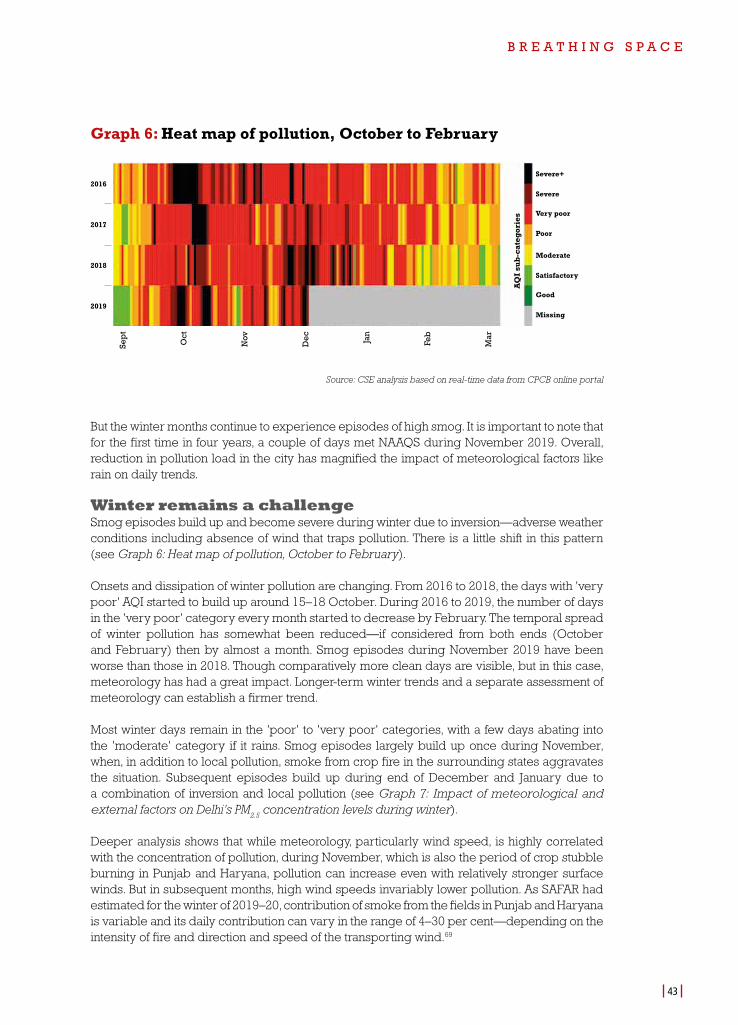
B R E A T H I N G S P A C E
43
Graph 6: Heat map of pollution, October to February
Severe+
Moderate
Very poor
Good
Severe
Satisfactory
Poor
Missing
Sep
t
Oct
Nov
Dec Ja
n
Feb
Mar
2016
2017
2018
2019
Source: CSE analysis based on real-time data from CPCB online portal
But the winter months continue to experience episodes of high smog. It is important to note that for the first time in four years, a couple of days met NAAQS during November 2019. Overall, reduction in pollution load in the city has magnified the impact of meteorological factors like rain on daily trends.
Winter remains a challengeSmog episodes build up and become severe during winter due to inversion—adverse weather conditions including absence of wind that traps pollution. There is a little shift in this pattern (see Graph 6: Heat map of pollution, October to February).
Onsets and dissipation of winter pollution are changing. From 2016 to 2018, the days with 'very poor' AQI started to build up around 15–18 October. During 2016 to 2019, the number of days in the 'very poor' category every month started to decrease by February. The temporal spread of winter pollution has somewhat been reduced—if considered from both ends (October and February) then by almost a month. Smog episodes during November 2019 have been worse than those in 2018. Though comparatively more clean days are visible, but in this case, meteorology has had a great impact. Longer-term winter trends and a separate assessment of meteorology can establish a firmer trend.
Most winter days remain in the 'poor' to 'very poor' categories, with a few days abating into the 'moderate' category if it rains. Smog episodes largely build up once during November, when, in addition to local pollution, smoke from crop fire in the surrounding states aggravates the situation. Subsequent episodes build up during end of December and January due to a combination of inversion and local pollution (see Graph 7: Impact of meteorological and external factors on Delhi’s PM
2.5 concentration levels during winter).
Deeper analysis shows that while meteorology, particularly wind speed, is highly correlated with the concentration of pollution, during November, which is also the period of crop stubble burning in Punjab and Haryana, pollution can increase even with relatively stronger surface winds. But in subsequent months, high wind speeds invariably lower pollution. As SAFAR had estimated for the winter of 2019–20, contribution of smoke from the fields in Punjab and Haryana is variable and its daily contribution can vary in the range of 4–30 per cent—depending on the intensity of fire and direction and speed of the transporting wind.69
AQ
I su
b-c
ateg
orie
s
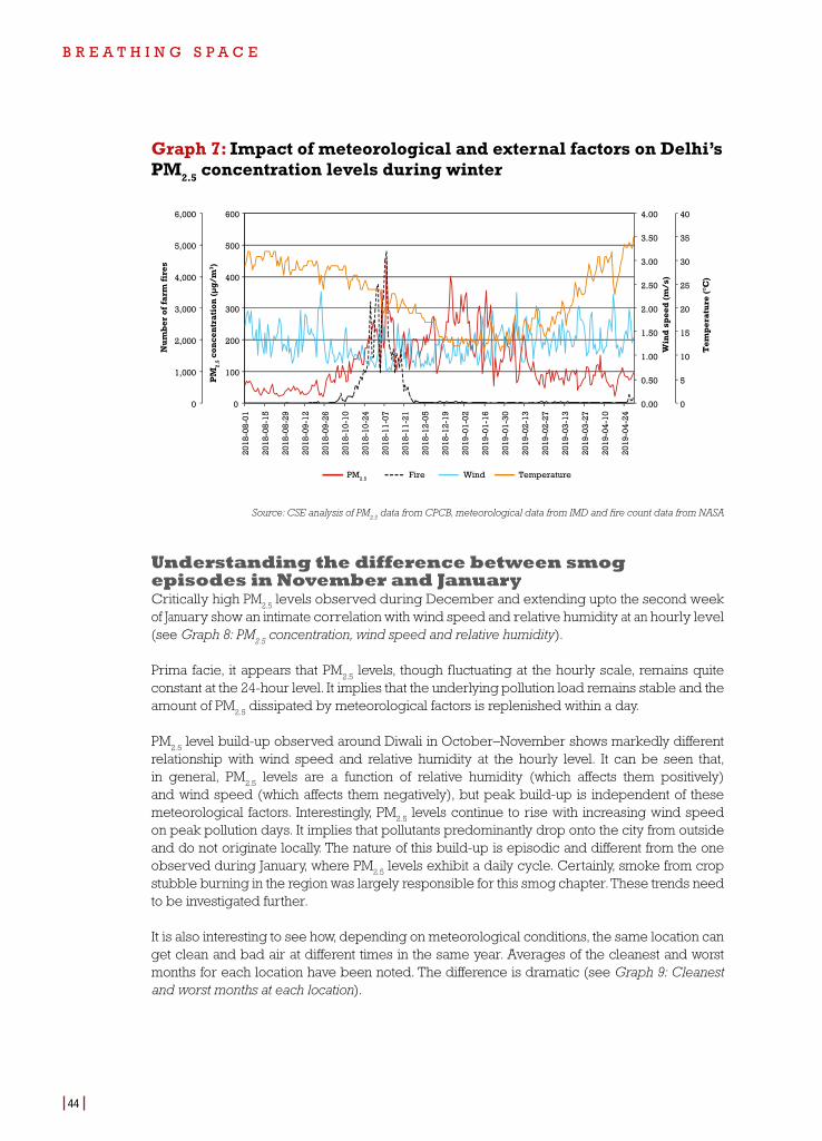
B R E A T H I N G S P A C E
44
Graph 7: Impact of meteorological and external factors on Delhi’s PM2.5 concentration levels during winter
0.00
0.50
1.00
1.50
2.00
2.50
3.00
3.50
4.00
0
100
200
300
400
500
600
0
1,000
2,000
3,000
4,000
5,000
6,000
2018
-08-
01
2018
-08-
15
2018
-08-
29
2018
-09-
12
2018
-09-
26
2018
-10-
10
2018
-10-
24
2018
-11-
07
2018
-11-
21
2018
-12-
05
2018
-12-
19
2019
-01-
02
2019
-01-
16
2019
-01-
30
2019
-02-
13
2019
-02-
27
2019
-03-
13
2019
-03-
27
2019
-04-
10
2019
-04-
24
Win
d s
pee
d (m
/s)
0
5
10
15
20
25
30
35
40
Tem
per
atu
re (°
C)
Nu
mb
er o
f far
m fi
res
PM
2.5 c
once
ntr
atio
n (µ
g/m
3 )
PM2.5 Fire Wind Temperature
Source: CSE analysis of PM2.5
data from CPCB, meteorological data from IMD and fire count data from NASA
Understanding the difference between smog episodes in November and JanuaryCritically high PM
2.5 levels observed during December and extending upto the second week
of January show an intimate correlation with wind speed and relative humidity at an hourly level (see Graph 8: PM
2.5 concentration, wind speed and relative humidity).
Prima facie, it appears that PM2.5
levels, though fluctuating at the hourly scale, remains quite constant at the 24-hour level. It implies that the underlying pollution load remains stable and the amount of PM
2.5 dissipated by meteorological factors is replenished within a day.
PM2.5
level build-up observed around Diwali in October–November shows markedly different relationship with wind speed and relative humidity at the hourly level. It can be seen that, in general, PM
2.5 levels are a function of relative humidity (which affects them positively)
and wind speed (which affects them negatively), but peak build-up is independent of these meteorological factors. Interestingly, PM
2.5 levels continue to rise with increasing wind speed
on peak pollution days. It implies that pollutants predominantly drop onto the city from outside and do not originate locally. The nature of this build-up is episodic and different from the one observed during January, where PM
2.5 levels exhibit a daily cycle. Certainly, smoke from crop
stubble burning in the region was largely responsible for this smog chapter. These trends need to be investigated further.
It is also interesting to see how, depending on meteorological conditions, the same location can get clean and bad air at different times in the same year. Averages of the cleanest and worst months for each location have been noted. The difference is dramatic (see Graph 9: Cleanest and worst months at each location).
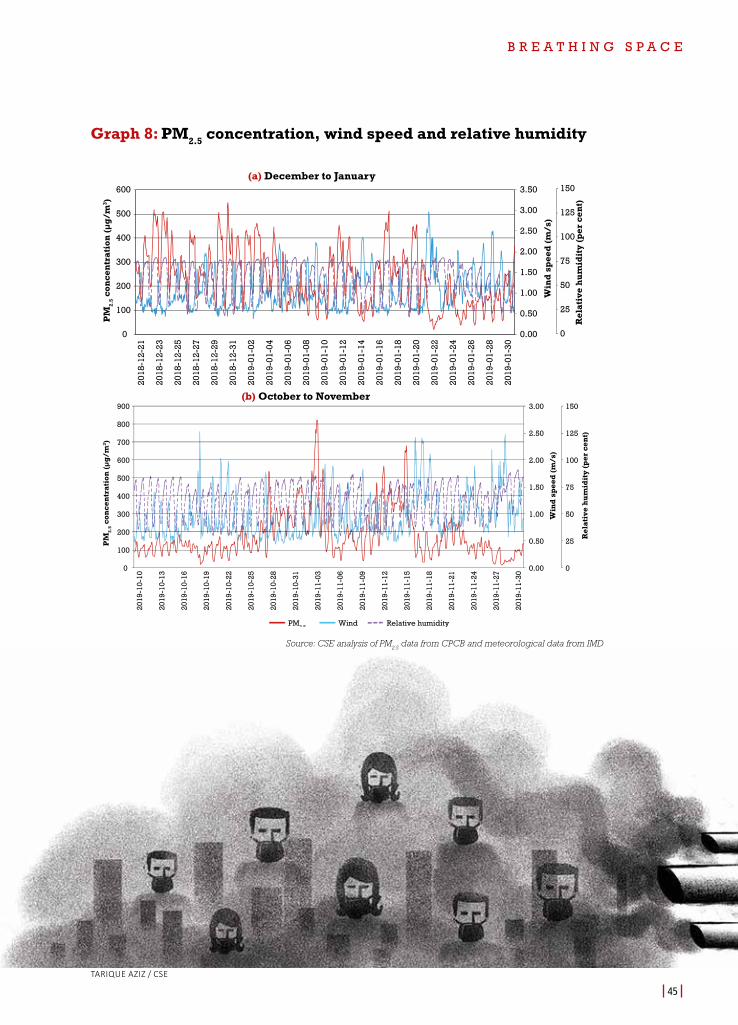
B R E A T H I N G S P A C E
45
Graph 8: PM2.5 concentration, wind speed and relative humidity
0.00
0.50
1.00
1.50
2.00
2.50
3.00
3.50
0
100
200
300
400
500
600
Win
d s
pee
d (m
/s)
PM
2.5 c
once
ntr
atio
n (µ
g/m
3 )
PM2.5 Wind Relative humidity
2018
-12-
21
2018
-12-
23
2018
-12-
25
2018
-12-
27
2018
-12-
29
2018
-12-
31
2019
-01-
02
2019
-01-
04
2019
-01-
06
2019
-01-
08
2019
-01-
10
2019
-01-
12
2019
-01-
14
2019
-01-
16
2019
-01-
18
2019
-01-
20
2019
-01-
22
2019
-01-
24
2019
-01-
26
2019
-01-
28
2019
-01-
30 0
25
50
75
100
125
150
Rel
ativ
e h
um
idit
y (p
er c
ent)
0.00
0.50
1.00
1.50
2.00
2.50
3.00
0
100
200
300
400
500
600
700
800
900
Win
d s
pee
d (m
/s)
0
25
50
75
100
125
150
Rel
ativ
e h
um
idit
y (p
er c
ent)
PM
2.5 c
once
ntr
atio
n (µ
g/m
3 )
PM2.5 Wind Relative humidity
2019
-10-
10
2019
-10-
13
2019
-10-
16
2019
-10-
19
2019
-10-
22
2019
-10-
25
2019
-10-
28
2019
-10-
31
2019
-11-
03
2019
-11-
06
2019
-11-
09
2019
-11-
12
2019
-11-
15
2019
-11-
18
2019
-11-
21
2019
-11-
24
2019
-11-
27
2019
-11-
30
Source: CSE analysis of PM2.5
data from CPCB and meteorological data from IMD
(a) December to January
(b) October to November
TARIQUE AZIZ / CSE
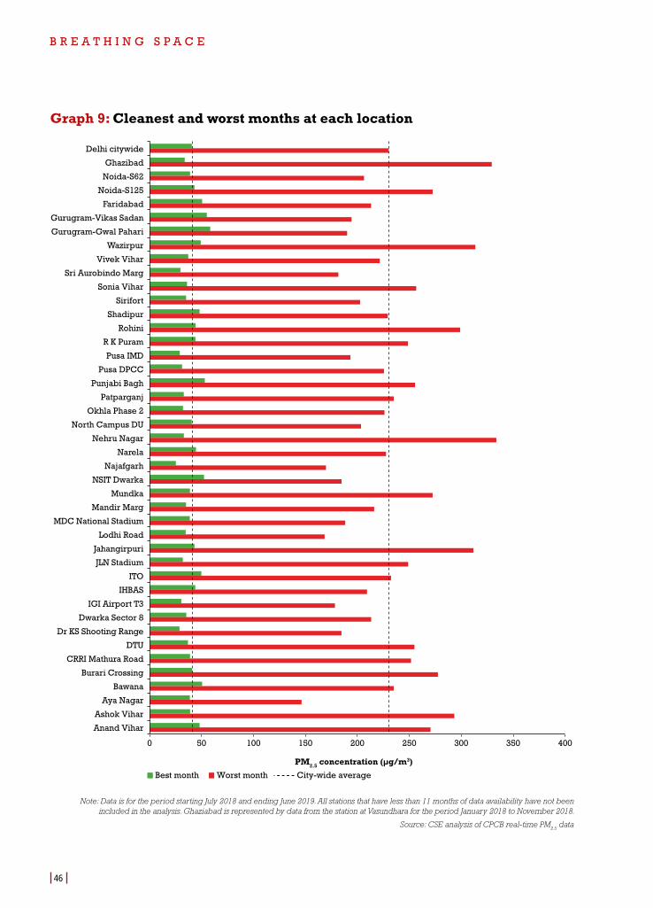
B R E A T H I N G S P A C E
46
Graph 9: Cleanest and worst months at each location
0 50 100 150 200 250 300 350 400
Anand Vihar
Ashok Vihar
Aya Nagar
Bawana
Burari Crossing
CRRI Mathura Road
DTU
Dr KS Shooting Range
Dwarka Sector 8
IGI Airport T3
IHBAS
ITO
JLN Stadium
Jahangirpuri
Lodhi Road
MDC National Stadium
Mandir Marg
Mundka
NSIT Dwarka
Najafgarh
Narela
Nehru Nagar
North Campus DU
Okhla Phase 2
Patparganj
Punjabi Bagh
Pusa DPCC
Pusa IMD
R K Puram
Rohini
Shadipur
Sirifort
Sonia Vihar
Sri Aurobindo Marg
Vivek Vihar
Wazirpur
Gurugram-Gwal Pahari
Gurugram-Vikas Sadan
Faridabad
Noida-S125
Noida-S62
Ghazibad
Delhi citywide
PM2.5 concentration (µg/m3)
Best month Worst month City-wide average
Note: Data is for the period starting July 2018 and ending June 2019. All stations that have less than 11 months of data availability have not been included in the analysis. Ghaziabad is represented by data from the station at Vasundhara for the period January 2018 to November 2018.
Source: CSE analysis of CPCB real-time PM2.5
data
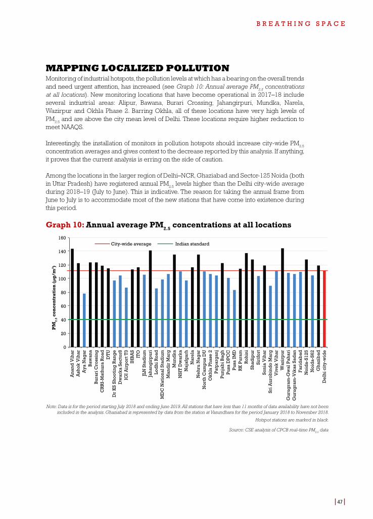
B R E A T H I N G S P A C E
47
MAPPING LOCALIZED POLLUTIONMonitoring of industrial hotspots, the pollution levels at which has a bearing on the overall trends and need urgent attention, has increased (see Graph 10: Annual average PM
2.5 concentrations
at all locations). New monitoring locations that have become operational in 2017–18 include several industrial areas: Alipur, Bawana, Burari Crossing, Jahangirpuri, Mundka, Narela, Wazirpur and Okhla Phase 2. Barring Okhla, all of these locations have very high levels of PM
2.5 and are above the city mean level of Delhi. These locations require higher reduction to
meet NAAQS.
Interestingly, the installation of monitors in pollution hotspots should increase city-wide PM2.5
concentration averages and gives context to the decrease reported by this analysis. If anything, it proves that the current analysis is erring on the side of caution.
Among the locations in the larger region of Delhi–NCR, Ghaziabad and Sector-125 Noida (both in Uttar Pradesh) have registered annual PM
2.5 levels higher than the Delhi city-wide average
during 2018–19 (July to June). This is indicative. The reason for taking the annual frame from June to July is to accommodate most of the new stations that have come into existence during this period.
Graph 10: Annual average PM2.5 concentrations at all locations
PM
2.5 c
once
ntr
atio
n (µ
g/m
3 )
0
20
40
60
Indian standardCity-wide average
80
100
120
140
160
Ana
nd V
ihar
A
shok
Vih
ar
Aya
Nag
ar
Baw
ana
Bura
ri C
ross
ing
C
RR
I-M
athu
ra R
oad
D
TU
Dr
KS
Shoo
ting
Ran
ge
Dw
arka
Sec
tor8
IG
I Air
por
t T3
IHBA
S IT
O
JLN
Sta
diu
m
Jaha
ngir
pur
i Lo
dhi
Roa
d
MD
C N
atio
nal S
tad
ium
M
and
ir M
arg
M
und
ka
NSI
T D
war
ka
Naj
afg
arh
Nar
ela
Neh
ru N
agar
N
orth
Cam
pus
DU
O
khla
Pha
se 2
Pa
tpar
gan
j Pu
njab
i Bag
h Pu
sa D
PCC
Pu
sa IM
D
RK
Pur
am
Roh
ini
Shad
ipur
Si
rifo
rt
Soni
a V
ihar
Sr
i Aur
obin
do
Mar
g
Viv
ek V
ihar
W
azir
pur
G
urug
ram
-Gw
al P
ahar
i G
urug
ram
-Vik
as S
adan
Fa
rid
abad
N
oid
a-S1
25
Noi
da-
S62
Gha
zib
ad
Del
hi c
ity-
wid
e
Note: Data is for the period starting July 2018 and ending June 2019. All stations that have less than 11 months of data availability have not been included in the analysis. Ghaziabad is represented by data from the station at Vasundhara for the period January 2018 to November 2018.
Hotspot stations are marked in black.
Source: CSE analysis of CPCB real-time PM2.5
data
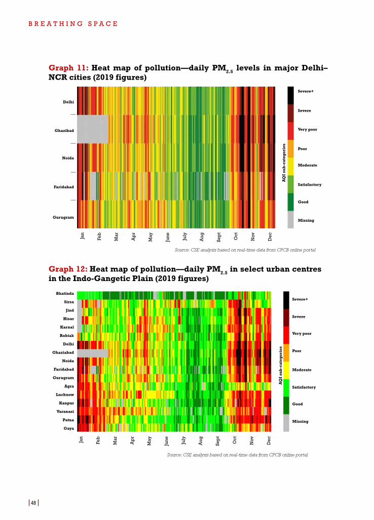
B R E A T H I N G S P A C E
48
Graph 11: Heat map of pollution—daily PM2.5 levels in major Delhi–NCR cities (2019 figures)
Severe+
Moderate
Very poor
Good
Severe
Satisfactory
Poor
Missing
Jan
Feb
Mar
Ap
r
May
June July
Aug
Sep
t
Oct
Nov
Dec
Source: CSE analysis based on real-time data from CPCB online portal
Delhi
Ghazibad
Noida
Faridabad
Gurugram
Graph 12: Heat map of pollution—daily PM2.5 in select urban centres in the Indo-Gangetic Plain (2019 figures)
Severe+
Moderate
Very poor
Good
Severe
Satisfactory
Poor
Missing
Jan
Feb
Mar
Ap
r
May
June July
Aug
Sep
t
Oct
Nov
Dec
Bhatinda
Sirsa
Jind
Hisar
Karnal
Rohtak
Delhi
Ghaziabad
Noida
Faridabad
Gurugram
Agra
Lucknow
Kanpur
Varanasi
Patna
Gaya
Source: CSE analysis based on real-time data from CPCB online portal
AQ
I su
b-c
ateg
orie
sA
QI
sub
-cat
egor
ies
B R E A T H I N G S P A C E
49
DELHI AND THE REGION
If long-term PM2.5
levels have stabilized and the curve has bent downwards, then why is Delhi still experiencing such severe smog episodes during winters? It is quite clear that with the entire northern belt and the region surrounding Delhi trapped in a thick blanket of smog due to winter inversion, Delhi will continue to face severe episodes even if there reduction in pollution at the city level.
Delhi–NCR-wide analysis shows that Delhi and NCR have identical seasonal PM2.5
profiles and the winter smog is uniformly distributed (see Graph 11: Heat map of pollution—daily PM
2.5
levels in major Delhi–NCR cities). Visual representation of the daily data of 2019 from Faridabad, Ghaziabad, Gurugram and Noida shows patterns which are almost identical to the ones observed in Delhi. The pollution levels in all these cities match closely. This is a clear indication that pollution is a larger regional issue.
But an analysis of winter pollution spread across the larger Indo-Gangetic Plain shows that urban centres with much lower annual PM
2.5 averages (compared to Delhi) also record peak
levels matching Delhi's around the same time as Delhi does (see Graph 12: Heat map of pollution—daily PM
2.5 levels in select urban centres in the Indo-Gangetic Plain and Smogged
Indo-Gangetic Plain).
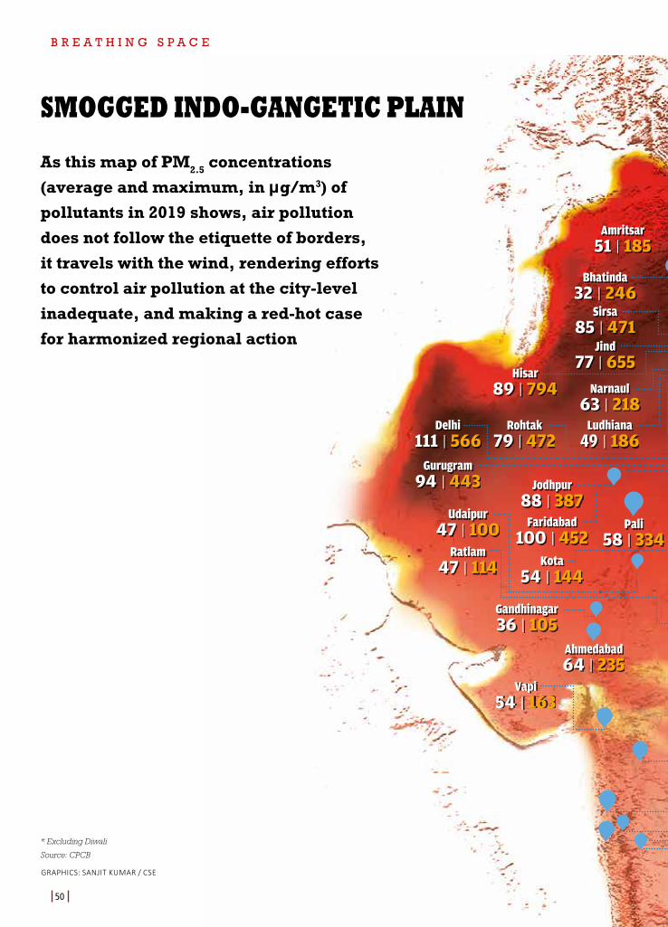
B R E A T H I N G S P A C E
50
Bhatinda32 | 246
Ludhiana49 | 186
Rohtak79 | 472
Gurugram94 | 443
Faridabad100 | 452
Hisar89 | 794
Delhi111 | 566
Kota54 | 144
Udaipur47 | 100
Amritsar51 | 185
Gandhinagar36 | 105
Ahmedabad64 | 235
Jodhpur88 | 387
Ratlam47 | 114
Pali58 | 334
Narnaul63 | 218
Sirsa85 | 471
Jind77 | 655
Vapi54 | 163
* Excluding Diwali
Source: CPCB
SMOGGED INDO-GANGETIC PLAIN
As this map of PM2.5 concentrations (average and maximum, in µg/m3) of pollutants in 2019 shows, air pollution does not follow the etiquette of borders, it travels with the wind, rendering efforts to control air pollution at the city-level inadequate, and making a red-hot case for harmonized regional action
GRAPHICS: SANJIT KUMAR / CSE
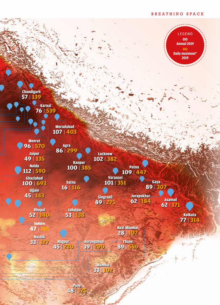
B R E A T H I N G S P A C E
51
Satna16 | 116
Varanasi101 | 351
Kanpur100 | 385
Singrauli89 | 275
Karnal76 | 539
Moradabad107 | 403
Noida112 | 590
Ghaziabad100 | 693
Agra86 | 299
Lucknow102 | 382
Meerut96 | 570
Chandigarh57 | 139
Jaipur49 | 135
Bhopal52 | 140
Jabalpur53 | 138
Navi Mumbai28 | 107
Mumbai33 | 102
Pune48 | 125
Thane89 | 550
Nashik33 | 127 Aurangabad
39 | 290
Ujjain45 | 143
Indore47 | 116
Nagpur45 | 230
Asansol62 | 171
Kolkata77 | 314
Jorapokhar62 | 184
Gaya89 | 307
Patna109 | 447
LEGEND00
Annual 201900
Daily maximum* 2019
B R E A T H I N G S P A C E
52
3(B). WHAT DELHI HAS DONE AND WHAT IT STILL MUST DO
The decennial analysis of air pollution (2010–19) shows stabilization and downward trend in Delhi’s particulate pollution levels. It also shows that the number of cleaner days has increased over time. Several locations reflect this downward trend. Winter pollution is setting in later and thinning out earlier.
Although these are optimistic signs, there is still a long way to go before Delhi’s air quality can even be close to clean. The composite average of the five oldest stations (with the most consistent data and data completeness) shows a reduction of about a quarter since 2012–14 levels, but this means there is need for another 67 per cent curtailment if the city is to meet PM
2.5 NAAQS. If data from the worst monitoring station is considered, Delhi still has to reduce
PM2.5
pollution by 75 per cent from the current baseline (2017–19). So, even as the analysis shows that action to combat air pollution has resulted in a clear downward trend, we still have miles to go.
Tracking changes in Delhi has become necessary to understand the successive stages of action. This will provide insight into the nature of drastic and disruptive action needed in future.
FIRST GENERATION ACTION ON AIR POLLUTION: 1998–2003
First generation action was driven by the urgency to find relief from the choking haze of pollution. A series of Supreme Court directives in multiple public interest litigations on air pollution led to eviction of big, polluting industrial units outside the city; introduction of largest ever natural gas (CNG) vehicle programme for public transport that replaced diesel run buses, mostly taxis, autos and small commercial vehicles; phase-out of old commercial vehicles; improvement in emissions standards for vehicles; and other such measures. Initially, this stabilized and arrested the pollution curve, but some of these gains were subsequently undermined as action slowed down and polltion kept increasing. Environment Pollution (Prevention and Control) Authority (EPCA) was set up under the direction of Supreme Court in 1998. It has been instrumental in taking forward these measures further. EPCA is responsible for recommending measures to the Supreme Court and monitoring implementation of the court's orders. It also issues directions for control of air pollution.
SECOND GENERATION ACTION ON AIR POLLUTION: 2015 ONWARDS
From 2015, momentum started to build up again. In this phase, multi-sectoral and diverse actions were initiated. During 2017–18, the Supreme Court directed the government to notify a Graded Response Action Plan (GRAP) for emergency interventions during smog episodes and a Comprehensive Action Plan (CAP) for sustained short- and long-term action across all sectors in Delhi–NCR. The implementation of GRAP is being monitored by EPCA. Relevant ministries of the Central government and departments of the governments of Delhi–NCR are implementing CAP. Simultaneously, several sector-specific measures have been implemented, aiming to promote clean fuel and technology transition across all sectors, catalyze mobility
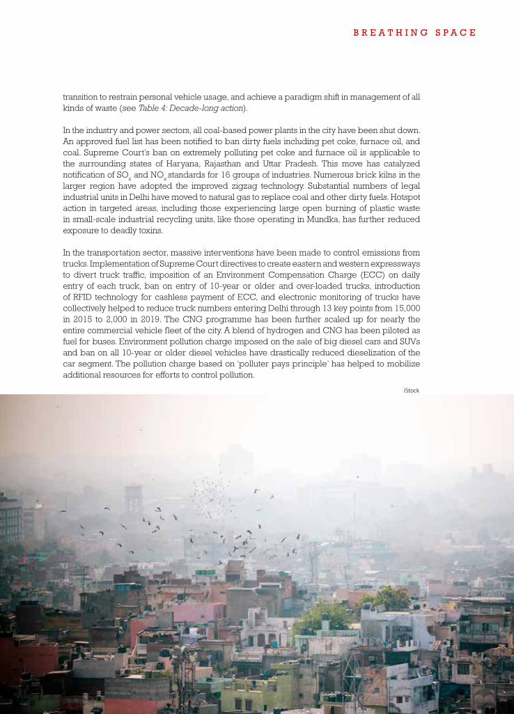
B R E A T H I N G S P A C E
53
transition to restrain personal vehicle usage, and achieve a paradigm shift in management of all kinds of waste (see Table 4: Decade-long action).
In the industry and power sectors, all coal-based power plants in the city have been shut down. An approved fuel list has been notified to ban dirty fuels including pet coke, furnace oil, and coal. Supreme Court’s ban on extremely polluting pet coke and furnace oil is applicable to the surrounding states of Haryana, Rajasthan and Uttar Pradesh. This move has catalyzed notification of SO
x and NO
x standards for 16 groups of industries. Numerous brick kilns in the
larger region have adopted the improved zigzag technology. Substantial numbers of legal industrial units in Delhi have moved to natural gas to replace coal and other dirty fuels. Hotspot action in targeted areas, including those experiencing large open burning of plastic waste in small-scale industrial recycling units, like those operating in Mundka, has further reduced exposure to deadly toxins.
In the transportation sector, massive interventions have been made to control emissions from trucks. Implementation of Supreme Court directives to create eastern and western expressways to divert truck traffic, imposition of an Environment Compensation Charge (ECC) on daily entry of each truck, ban on entry of 10-year or older and over-loaded trucks, introduction of RFID technology for cashless payment of ECC, and electronic monitoring of trucks have collectively helped to reduce truck numbers entering Delhi through 13 key points from 15,000 in 2015 to 2,000 in 2019. The CNG programme has been further scaled up for nearly the entire commercial vehicle fleet of the city. A blend of hydrogen and CNG has been piloted as fuel for buses. Environment pollution charge imposed on the sale of big diesel cars and SUVs and ban on all 10-year or older diesel vehicles have drastically reduced dieselization of the car segment. The pollution charge based on ‘polluter pays principle’ has helped to mobilize additional resources for efforts to control pollution.
iStock
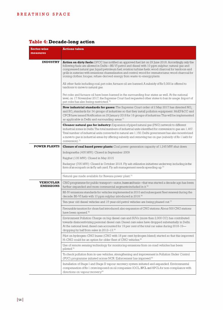
B R E A T H I N G S P A C E
54
Table 4: Decade-long action Sector-wise measures
Actions taken
INDUSTRY Action on dirty fuels: DPCC has notified an approved fuel list on 29 June 2018. Accordingly, only the following fuels are allowed in Delhi—BS-VI petrol and diesel with 10 ppm sulphur; natural gas and compressed natural gas; liquid petroleum fuel; aviation turbine fuels; wood charcoal for tandoors and grills in eateries with emissions channelization and control; wood for crematoriums; wood charcoal for ironing clothes; biogas; refuse-derived energy from waste-to-energy plants.
All other fuels including coal, pet coke, furnace oil are banned. A subsidy of Rs 5,000 is offered to tandoors to move to natural gas.
Pet coke and furnace oil have been banned in the surrounding four states as well. At the national level, on 17 November 2017, the Supreme Court had requested other states to ban its usage. Import of pet coke has also being restricted.70
New industrial standards for gases: The Supreme Court order of 2 May 2017 has directed NOx
and SOx standards for 34 groups of industries so that they install pollution equipment. MoEF&CC and CPCB have issued Notification on 29 January 2018 for 16 groups of industries. This will be implemented as applicable in Delhi and surrounding areas.71
Cleaner natural gas for industry: Expansion of piped natural gas (PNG) network to different industrial zones in Delhi. The total numbers of industrial units identified for conversion to gas are 1,467. Total number of industrial units converted to natural are 1,150. Delhi government has also incentivized a move to gas in industrial areas by offering subsidy and removing tax on gas (subsidy of Rs 1 lakh for conversion).72
POWER PLANTS Closure of coal based power plants: Coal power generation capacity of 1,245 MW shut down
Indraprastha (405 MW): Closed in September 2009
Rajghat (135 MW): Closed in May 2015
Badarpur (705 MW): Closed in October 2018. Fly ash utilization initiatives underway, including in the form of an ecopark on its fly ash yard. Fly ash management needs speeding up.73
Natural gas made available for Bawana power plant.74
VEHICULAR EMISSIONS
CNG programme for public transport—autos, buses and taxis—that was started a decade ago has been further expanded and more commercial segments included in it.75
BS-IV emissions standards for vehicles implemented in 2010 and subsequent fleet renewal during the decade. BS-VI fuels with 10 ppm sulphur introduced in 2018.76
Ten-year old diesel vehicles and 15 year-old petrol vehicles are being phased out.77
Favourable taxation for clean fuel introduced; also expansion of CNG stations. About 500 CNG stations have been opened.78
Environment Pollution Charge on big diesel cars and SUVs (more than 2,000 CC) has contributed towards disincentivizing personal diesel cars. Diesel cars sales have dropped substantially in Delhi. At the national level, diesel cars accounted for 19 per cent of the total car sales during 2018-19—dropping by half from sales in 2012–13.79
Pilot on hydrogen–CNG buses (CNG with 18 per cent hydrogen blend) started so that this improved H–CNG could be an option for older fleet of CNG vehicles.80
Use of remote sensing technology for monitoring emissions from on-road vehicles has been piloted.81
To check pollution from in-use vehicles, strengthening and improvement in Pollution Under Control (PUC) programme initiated across NCR. Enforcement has improved.82
Installation of Stage I and Stage II vapour recovery system initiated and expanded. Environmental compensation of Rs 1 crore imposed on oil companies: IOCL, BPCL and HPCL for non-compliance with directions on vapour recovery.83
B R E A T H I N G S P A C E
55
SPECIFIC ACTION ON
TRUCKS: A HIGH-
POLLUTING SEGMENT OF
VEHICLES
The long-awaited bypass roads to divert commercial traffic built: The construction of Eastern Peripheral Expressway and Western Peripheral Expressway (EPE and WPE) was ordered in 2005 and they have been made functional in 2018–19, which has allowed commercial and extremely polluting trucks to bypass the city. It is estimated that about 60,000 trucks are using the bypasses.84
To deter non-destined truck traffic, the country’s first congestion charging introduced in 2015. Environment Compensation Charge (ECC) on each category of commercial vehicles imposed at the time of entry into the city.85
Restriction on entry of 10-year old trucks and introduction of weigh-in-motion bridges at the border to control overloading of trucks.86
Introduction of RFID at 13 entry points in Delhi for cashless ECC payment, making the congestion charge effective. RFID tags are mandatory for commercial vehicles. This has reduced congestion at toll gates. The latest estimate shows that the number of trucks entering Delhi from 13 key entry points has reduced from 15,000 to 2,000.87
PUBLIC TRANSPORT
After stagnation and decline in bus numbers and passengers, procurement of new buses has started. As per the Outcome Status presented to the Delhi Assembly in February 2019, the average daily ridership of DTC buses has increased by two lakh compared to 2016–17. The average ridership of DTC buses is 42.03 lakh. DTC bus numbers have reduced. Ridership numbers of cluster bus scheme is not available. Bus parking constraint is being addressed.88
NCR reciprocal agreement—autos and buses allowed to run across borders in entire NCR draft in 2008 and effective from 2010. It is up for renewal.89
The ridership in the metro has increased from 1,259,000 in 2010–11 to 2,708,376 in 2018–19. Operational routes have increased from 165.5 km in 2010–11 to 373 km in 2018–19;. Rolling stock has increased from 844 in 2010–11 to 2,194 in 2018–19.90
Parking policy as a demand management tool has been notified. Pilot schemes on parking area management plans have been initiated.91
CONSTRUC-TION AND
DEMOLITION WASTE AND
DUST
Checklist for dust control at construction sites made so that enforcement is improved. Penalty on violation initiated. According to the latest Economic Survey, in 2019 DPCC imposed fines to the tune of Rs 3.5 crore with respect to dust control. DPCC has imposed fines on construction projects that have obtained environmental clearance (with a built-up area of more than 20,000 sq meter).92
The Construction and Demolition Waste Management Rules, 2016 notified and BIS rules modified in 2014 to allow use of recycled C&D waste in building construction.93
There are 60 mechanized road sweeping machines in Delhi.94
Environmental compensation of Rs 1 crore has been imposed on municipal bodies (New Delhi, South, East, North and Cantonment Board) over open dumping and burning of garbage and C&D waste vide directions dated 16 January 16 2019 under section 31A of the Air (Prevention and Control of Pollution) Act, 1981.95
The city has expanded recycling capacity of its C&D waste recycling plant at Burari from 500 MTD to 2,000 MTD. It has also added two more recycling plants . Together, the three plants had recycled five million tonnes of waste by the end of 2019.96
WASTE BURNING
Solid Waste Management Rules and Regulations 2016 notified.97
Delhi bye-laws amended based on these rules and notified in January 2017. To be implemented.98
The city has over 2,300 waste dumps—neighbourhood structures to collect and store waste. Over 80 per cent of the waste is processed through incineration, though studies show that the calorific value of Delhi’s waste does not support incineration.99
Recently, Delhi fought a bitter battle to stop large-scale burning of plastics in Mundka area that used to produce enormous quantities of poisonous gases. Now factories have been linked with waste to energy plant for safe removal and disposal of plastic waste in that area. It is estimated that as a result of this initiative about 80,000 tonnes of plastic waste have been removed for safer disposal that otherwise would have burnt in the open.100
Only about 10 per cent of waste in the city is segregated, and segregation is restricted to a few institutions and colonies. Twelve wards have been selected as model wards. To prevent littering, 6,000 roadside twin bins have been procured.101
MONITORING AND GRADED
RESPONSE ACTION PLAN
(GRAP)
Air quality monitoring stations expanded to 38 in Delhi and to over 50 in the larger region.102
Early Warning System and forecasting for Delhi launched in October 2018.103
GRAP, targeting key sources of pollution during emergencies, has been implemented during the winters of 2017–18 and 2018–19 and 2019–20: Short-term measures taken during smog episodes include shutting down power plants, closing industrial units using coal, ban on construction, ban on brick kilns, action on waste burning and construction, and mechanized cleaning of road dust. Limited scheme of odd and even scheme is also part of it.104
Source: Compiled by CSE from various sources
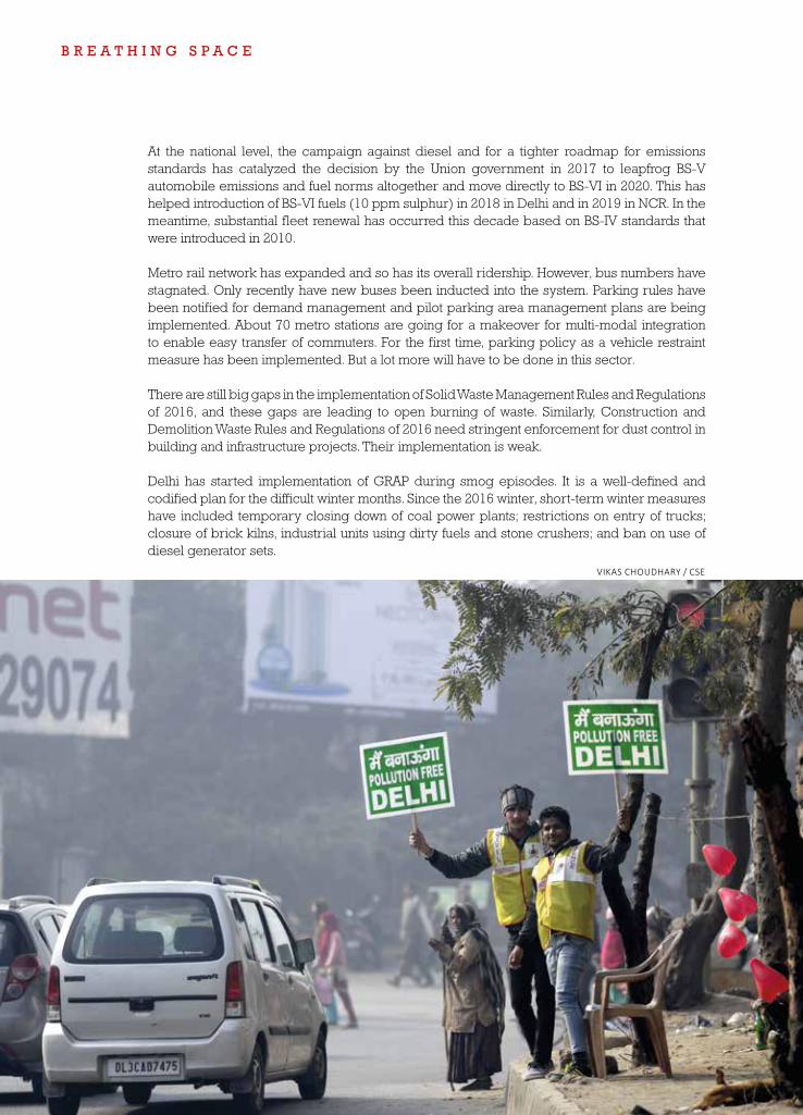
B R E A T H I N G S P A C E
56
At the national level, the campaign against diesel and for a tighter roadmap for emissions standards has catalyzed the decision by the Union government in 2017 to leapfrog BS-V automobile emissions and fuel norms altogether and move directly to BS-VI in 2020. This has helped introduction of BS-VI fuels (10 ppm sulphur) in 2018 in Delhi and in 2019 in NCR. In the meantime, substantial fleet renewal has occurred this decade based on BS-IV standards that were introduced in 2010.
Metro rail network has expanded and so has its overall ridership. However, bus numbers have stagnated. Only recently have new buses been inducted into the system. Parking rules have been notified for demand management and pilot parking area management plans are being implemented. About 70 metro stations are going for a makeover for multi-modal integration to enable easy transfer of commuters. For the first time, parking policy as a vehicle restraint measure has been implemented. But a lot more will have to be done in this sector.
There are still big gaps in the implementation of Solid Waste Management Rules and Regulations of 2016, and these gaps are leading to open burning of waste. Similarly, Construction and Demolition Waste Rules and Regulations of 2016 need stringent enforcement for dust control in building and infrastructure projects. Their implementation is weak.
Delhi has started implementation of GRAP during smog episodes. It is a well-defined and codified plan for the difficult winter months. Since the 2016 winter, short-term winter measures have included temporary closing down of coal power plants; restrictions on entry of trucks; closure of brick kilns, industrial units using dirty fuels and stone crushers; and ban on use of diesel generator sets.
VIKAS CHOUDHARY / CSE
B R E A T H I N G S P A C E
57
Air quality and health gains from the ongoing action in Delhi have not been studied well. The hope is that more such studies will be carried out now, to understand the impact of action against air pollution. This will enable policy makers to assess how much more needs to be done for the next big cut. So far, very few studies have attempted to assess the impact of action either on emissions rates at source or on the larger air quality of Delhi.
During the earlier decade (2000–10), a few studies were carried out to show the impact of action on air quality. CPCB had estimated that after the implementation of the CNG programme, particulate levels had dropped by about 24 per cent from the 1996 levels.105 A study by the Washington DC-based Resources for the Future,106 found that of all the different interventions made to combat pollution in Delhi, the CNG programme had the maximum impact as buses travel more kilometers and contribute more to the pollution load. A study done at the Jawaharlal Nehru University, Delhi found perceptible drop in polycyclic aromatic hydrocarbons—a group of very toxic pollutants—in Delhi’s air immediately after the introduction of the CNG programme.107 A World Bank study of 2004 showed that first-generation measures in Delhi and Mumbai, that also include CNG programmes, have helped reduce the number of premature deaths annually—by at least 3,629 in Delhi.108
There are no studies post-2010 on the impact of action on air quality. SAFAR estimates put the absolute change in PM
2.5 emissions (and not concentration) in the last eight years at 15 per
cent (comparing data for 2010 and 2018). It has identified the sectors showing increase and decrease in emissions. While the contribution of the residential sector has decreased by 64 per cent, emissions from industry have increased by 48 per cent, and those from the transport sector have increased by 40 per cent. Emissions from other sources have also increased nine times.109
It is hoped that more detailed assessments of impact of action and meteorology on air pollution trends will be undertaken in the future to strengthen future roadmaps.
MULTI-SECTORAL ACTION IN DELHI: LESSONS
The big message is that even though action against air pollution in Delhi has not been unsubstantial and has helped bend the pollution curve downwards, yet the action is not enough—certainly not on a scale that is needed for round-the-year clean air. An even more challenging aspect of the change achieved so far is the difficulty in getting each of the measures implemented. Nearly all the measures implemented so far have been strongly contested in the Supreme Court; there have been misinformation campaigns to obstruct their formulation and implementation, and to confuse or delay action; there have also been infrastructure deficits and institutional laxity that have slowed down action. As a result, the city has lost a lot of precious time—from one–three years to upto 10 years time lag can be attributed to different action points.
There is clearly a need for sensitization and deepening of awareness so that when solutions are contested, public and policy support can be mustered quickly to speed up change. If what has been implemented so far was difficult, future action for much deeper cuts in pollution will be even more disruptive and, therefore, harder to implement. How do we ensure that the reduction in PM
2.5 levels by more than 65 per cent overall and by over 75 per cent from the worst trend
to meet NAAQS takes place quickly? This reduction target is much more ambitious than NCAP targets. The breadth of the answer to this question is our breathing space.
Upscale clean energy and technology transition in Delhi and NCR: Need massive scaleup of clean energy and technology transition in industry and power sectors with stringent compliance systems across the region. This will have to be built on the action taken so far.
B R E A T H I N G S P A C E
58
Approved fuel lists to eliminate coal and dirty fuel streams, and new NOx and SO
x standards to
tighten PM emissions limits at industrial boilers need to be enforced. Strong hotspot monitoring and localized action also needs to be ensured. The specific problems of informal sources of pollution; and fugitive emissions from small-scale units, material handing, and open burning of industrial waste, including plastics waste, need to be addressed.
The industry sector continues to have an enormous problem of small-scale and unauthorized units. In August 2019, Delhi State Industrial Infrastructure Development Corporation listed 51,837 units operating in non-conforming areas.110 This is in addition to the substantial number of unauthorized household units. Customized solutions determining permission criteria, siting, clean fuels and emissions control will be needed for this sector.
Regional action on power plants to implement new emissions standards and move to natural gas: While Delhi has closed all coal-power plants, NCR-based coal-power plants will have to meet new emissions standards. NCR will also require a roadmap for replacing coal with natural gas for power generation. But transition from coal to natural gas in power plants (like in industry sector) will require a fuel pricing policy to keep natural gas competitively priced vis-à-vis coal. Moreover, a fly ash recycling policy is in place but will require enforcement at scale.
Transform public transport at scale and enforce vehicle restraint measure in Delhi–NCR: So far, the action on mobility and vehicle restraint has been the weakest in Delhi–NCR. In pursuit of the measures in the Delhi Master Plan 2020-21, it must be ensured that least 80 per cent of all daily travel trips are by public transport. This will require massive augmentation of public transport infrastructure, augmentation of bus numbers, reliable and affordable bus services connecting all neighbourhoods, integration of all systems—metro and buses—supported by walking and cycling infrastructure and last-mile connectivity at scale.
Currently, action has been initiated as part of the Comprehensive Action Plan for multi-modal integration through physical integration of metro stations and fare integration and augmentation of bus and metro services. Delhi has notified the first ever parking rules as a demand management measure for enforcement of parking area management plans across the city with maximum parking caps and variable pricing. This needs implementation at scale. Take action to control real-world emissions from vehicles and implement zero emissions mandate: From April 2020, BS-VI emissions standard will be implemented nation-wide. The next big step is to make on-road emissions management BS-VI-ready. Physical checks of advanced emissions control systems to prevent tampering; integration of remote sensing measurements with on-road emissions inspection to address gross polluters; and characterization of emissions of the fleet must be ensured. An emissions recall programme and strong deterrence for emissions frauds must be enforced. Otherwise, even after meeting advanced emissions standards, new vehicles may unleash uncontrolled emissions. These measures, especially application of remote sensing measurements, will have to be supported by the requisite amendments to the Central Motor Vehicle Rules.
Simultaneously, efforts must be made to leapfrog to electric mobility to cut down exposures. Delhi has already issued an electric vehicle policy, which needs clear milestones to meet the target of 25 per cent electric vehicle penetration in the city market by 2023.111 At the same time, the national government needs to adopt a zero emissions mandate to bring clarity to the market and to ensure adoption of the right incentives and instruments to accelerate the transition.
B R E A T H I N G S P A C E
59
Ensure effective implementation of waste management—solid waste and construction and demolition waste: Delhi has already amended municipal bye-laws in accordance with the Solid Waste Management Rules and Regulations of 2016, that require an infrastructure and enforcement strategy for decentralized solid waste management, recycling, landfill management and consumer charges. But implementation will have to be scaled up. Even though relevant rules are in place, there is enormous infrastructure deficit for segregated collection and transportation, recycling facilities and reuse strategies. This holds true for dust control measures in construction, and recycling of construction and demolition waste as well, where enforcement is needed at scale.
Need strong action in pollution hotspots: Under the direction of the Supreme Court, about 14 pollution hotspots have been identified in Delhi–NCR, based on a local survey. The survey shows that most of these hotspots face serious problems of open burning of industrial and solid waste, unpaved roads and movement of heavy traffic, construction activities, industrial emissions, etc. Hotspot action plans have been prepared and their implementation is underway. Local solutions will have to be implemented not only to reduce the high local level of pollution but also to reduce exposure of local communities. Often, these communities belong to poorer sections. Hotspots also influence the variability in the ambient concentration of PM in a city that otherwise has quite uniform terrain.
Eliminate use of solid fuels in households: Delhi has seen substantial reduction in use of solid fuels in households. SAFAR estimates a reduction in emissions rates from household fuels by about 63 per cent from 2010 levels. Pressure needs to be kept up, to achieve total elimination in Delhi as well as the larger NCR. While government schemes like Ujjwala have helped to scale up access to clean fuels, the sustained use and refill of alternatives remains a challenge, given the poverty levels and pricing of such alternatives.
Ensure enforcement, incentivization, deterrence and compliance: This is the only way to ensure that Delhi and the larger region continue to harvest sustained air quality gains. Implementation of the Comprehensive Action Plan will require effective planning, implementation, enforcement, compliance, and institutional capacity and accountability for solutions across all key sectors of pollution. A strong deterrence policy will have to be designed for each sector. However, this issue is not specific to Delhi. In addition to state-level action, it requires reform in the national legal framework for compliance. Comprehensive Action Plan of Delhi has been notified by MoEF&CC under Section 3 and 5 of the Environment Protection Act, that confers enormous power and authority. These powers will have to be exercised. Several other legal reforms are needed to enable multi-sectoral action and to allow strong civil penalty under the Air Act.
Need regional action: Action needs scale and uniform implementation across the NCR and the even larger Indo-Gangetic Plain (as well as other regions). At the national level, regional plans are needed, with an appropriate legal framework. Responsibilities will have to be fixed based on up-wind and down-wind locations, and good neighbour policies for state governments established, to create vertical and horizontal accountability across regions.
As the 122 'non-attainment' cities begin implementation of CAPs under NCAP, it is important to learn from Delhi’s experience. What Delhi has done so far was tough to push across, what is needed to achieve the next big cut in pollution will be even harder to achieve. While we need to celebrate action, we also need to build stronger support for harder and more disruptive action.
B R E A T H I N G S P A C E
60
REFERENCES AND ENDNOTES
1. Nikunja K Sundaray and Shruti Rai Bhardwaj 2019. National Clean Air Programme, Ministry of Environment, Forest & Climate Change, Government of India, New Delhi
2. Anon 2019. O.A. No. 681/2018 (Date of hearing: 6 August 2019), National Green Tribunal, New Delhi
3. Nikunja K Sundaray and Shruti Rai Bhardwaj 2019. National Clean Air Programme, Ministry of Environment, Forest & Climate Change, Government of India, New Delhi
4. Anon 2019. O.A. No. 681/2018 (Date of hearing: 6 August 2019), National Green Tribunal, New Delhi
5. Anon 2009. National Ambient Air Quality Standards Notification, Central Pollution Control Board, New Delhi
6. Central Control Room for Air Quality Management, Delhi–NCR. Available at https://app.cpcbccr.com/ccr/#/login, as accessed on 14 January 2020
7. Anon 2019. O.A. No. 681/2018 (I.A. No. 411/2019) with O.A. No.10/2019 (EZ) (Date of Order: 20 November 2019), National Green Tribunal, New Delhi
8. Central Control Room for Air Quality Management, Delhi–NCR. Available at https://app.cpcbccr.com/ccr/#/login, as accessed on 14 January 2020
9. Based on the estimated cost of setting up a real-time station: Rs 3 crore.
10. Anon 2013. “Final rule”, Federal Register Volume 78, Issue 10 (15 January 2013), Office of the Federal Register, National Archives and Records Administration, US
11. Anon 2008. Directive 2008/50/EC of The European Parliament and of The Council of 21 May 2008 on ambient air quality and cleaner air for Europe, Official Journal of the European Union, Brussels, Belgium
12. Dian Ding et al 2019. “Estimated contribution of emissions control, meteorological factors, population growth and changes in baseline mortality to reductions in ambient PM2.5 and PM2.5-related mortality in China, 2013–17”, Environmental Health Perspectives, National Institute of Environmental Health Sciences, US
13. Anon 2019. Economic Survey of Delhi 2018–19, Planning Department, Government of National Capital Territory of Delhi
14. Anon 2019. Delhi Government Performance: 2015–19, Dialogue and Development Commission of Delhi, Government of National Capital Territory of Delhi
15. Anon 2018. Notification List of Approved Fuels in the National Capital Territory of Delhi, Delhi Pollution Control Committee, New Delhi
16. Anon 2019. EPCA Report No. 106: Special report on pollution hotspots in NCR with request for urgent directions to improve enforcement and pollution control, 18 October 2019, Environment Pollution (Prevention and Control) Authority for NCR, New Delhi
B R E A T H I N G S P A C E
61
17. Anon 2018. Delhi and NCR Air Pollution Report Card 2017–18: A status report, Environment Pollution (Prevention & Control) Authority for Delhi and Centre for Science and Environment, New Delhi
18. Anon 2018. BS-VI fuel will bring down sulphur level by 80 per cent from current BS-IV levels, says Dharmendra Pradhan, Ministry of Petroleum and Natural Gas, Press Information Bureau, Government of India, New Delhi
19. Anon 2020. EPCA Report No. 109, Environment Pollution (Prevention and Control) Authority for NCR, New Delhi (Based on the difference between the estimate provided by South Delhi Municipal Corporation in January 2020 and an independent study conducted in 2015)
20. Anon 2018. “Report No. 92 Submitted By EPCA (Special Report On NCR Air Pollution), 29 October 2018”, Writ Petition(s) (Civil) No.(s).13029/1985, Supreme Court of India, New Delhi
21. Anon 2019. “Report No. 97 Submitted By EPCA, 6 September 2019”, Writ Petition(s)(Civil) No(s).13029/1985, Supreme Court of India, New Delhi
22. Anon 2017. Notification, Graded Response Action Plan, Ministry of Environment, Forest and Climate Change, Government of India, New Delhi
23. Anon 2019. Ambient Air Quality Monitoring Data for the Year 2018 (Manual monitoring under National Ambient Air Quality Monitoring Programme), Central Pollution Control Board, New Delhi
24. Anon 2019. “PM2.5 Design Values, 2018 (XLSX)”. United States Environmental Protection Agency, US. Available at https://www.epa.gov/air-trends/air-quality-design-values, as accessed on 5 February 2020
25. Sean M Raffuse et al 2007. Ambient Air Monitoring Network Assessment Guidance: Analytical Techniques for Technical Assessments of Ambient Air Monitoring Network, United States Environmental Protection Agency, US
26. Anon 2019. “Air Quality Statistics by City, 2018 (XLSX)”. United States Environmental Protection Agency, US. Available at https://www.epa.gov/air-trends/air-quality-cities-and-counties, as accessed on 5 February 2020
27. Anon 2019. “PM2.5 Design Values, 2018 (XLSX)". United States Environmental Protection Agency, US. Available at https://www.epa.gov/air-trends/air-quality-design-values, as accessed on 5 February 2020
28. Gufran Beig 2019. How Science of Forecasting Shapes Action, SAFAR, Indian Institute of Tropical Meteorology, Pune (additional details were sourced directly from SAFAR)
29. Anon 1997. Guidance for setting air quality standards: Report on a WHO Working Group, WHO Regional Office For Europe, Barcelona, Spain
30. Anon 2019. “PM2.5 Design Values, 2018 (XLSX)”. United States Environmental Protection Agency, US. Available at https://www.epa.gov/air-trends/air-quality-design-values, as accessed on 5 February 2020
31. Ibid
32. Anon 2003. National Ambient Air Quality Status Report, Central Pollution Control Board, New Delhi
B R E A T H I N G S P A C E
62
33. Anon 2015. Protocol for Data Transmission from CAAQM Stations Existing as on Date, IT Division, Central Pollution Control Board, New Delhi
34. Central Control Room for Air Quality Management, Delhi–NCR. Available at https://app.cpcbccr.com/ccr/#/login, as accessed on 14 January 2020
35. Anon 2018. 40 CFR Part 50—National Primary and Secondary Ambient Air Quality Standards. Available at https://www.govinfo.gov/content/pkg/CFR-2018-title40-vol2/xml/CFR-2018-title40-vol2-part50.xml, as accessed on 9 October 2019
36. Anon 1997. “Final rule”, Federal Register Volume 62, No. 138 (18 July 1997), Office of the Federal Register, National Archives and Records Administration, US
37. Anon 2013. “Final rule”, Federal Register Volume 78, Issue 10 (15 January 2013), Office of the Federal Register, National Archives and Records Administration, US
38. Ibid
39. Ibid
40. Anon 2012. Guidance Document On Achievement Determination Canadian Ambient Air Quality Standards For Fine Particulate Matter And Ozone, Canadian Council of Ministers of the Environment, Winnipeg, Manitoba, Canada
41. Anon 2002. Decision No 1600/2002/EC of the European Parliament and of the Council of 22 July 2002 laying down the Sixth Community Environment Action Programme, Council of the European Union and European Parliament, Brussels, Belgium
42. Anon 2008. Directive 2008/50/EC of The European Parliament and of The Council of 21 May 2008 on ambient air quality and cleaner air for Europe, Official Journal of the European Union, Brussels, Belgium
43. Ibid
44. Anon 2010. National Environment Protection (Ambient Air Quality) Measure: Technical Paper No. 8—Annual Reports, National Environment Protection Council, Commonwealth of Australia, Australia
45. Dian Ding et al 2019. “Estimated contribution of emissions control, meteorological factors, population growth and changes in baseline mortality to reductions in ambient PM2.5 and PM2.5-related mortality in China, 2013–17”, Environmental Health Perspectives, National Institute of Environmental Health Sciences, US
46. Anon 2018. 40 CFR Appendix N to Part 50—National Primary and Secondary Ambient Air Quality Standards. Available at https://www.govinfo.gov/content/pkg/CFR-2018-title40-vol2/xml/CFR-2018-title40-vol2-part50.xml, as accessed on 9 October 2019
47. Anon 2012. Guidance Document On Achievement Determination Canadian Ambient Air Quality Standards For Fine Particulate Matter And Ozone, Canadian Council of Ministers of the Environment, Winnipeg, Manitoba, Canada
48. Anon 2008. Directive 2008/50/EC of The European Parliament and of The Council of 21 May 2008 on ambient air quality and cleaner air for Europe, Official Journal of the European Union, Brussels, Belgium
B R E A T H I N G S P A C E
63
49. Anon 2010. National Environment Protection (Ambient Air Quality) Measure: Technical Paper No. 8—Annual Reports, National Environment Protection Council, Commonwealth of Australia, Australia
50. Anon 2017. "How is AQI calculated?", Central Pollution Control Board of India. Available at https://app.cpcbccr.com/ccr_docs/How_AQI_Calculated.pdf, as accessed on 9 October 2019
51. Nikunja K Sundaray and Shruti Rai Bhardwaj 2019. National Clean Air Programme, Ministry of Environment, Forest and Climate Change, Government of India, New Delhi
52. Anon 2018. 40 CFR Appendix N to Part 50—National Primary and Secondary Ambient Air Quality Standards. Available at https://www.govinfo.gov/content/pkg/CFR-2018-title40-vol2/xml/CFR-2018-title40-vol2-part50.xml, as accessed on 9 October 2019
53. Ibid
54. Anon 2017. 2017 Air Monitoring Network Plan, San Joaquin Valley Air Pollution Control District, California, US
55. Anon 2019. “PM2.5 Design Values, 2018 (XLSX)”. United States Environmental Protection Agency, US. Available at https://www.epa.gov/air-trends/air-quality-design-values, as accessed on 5 February 2020
56. Anon 2018. 40 CFR Part 58—Ambient Air Quality Surveillance. Available at https://www.ecfr.gov/cgi-bin/retrieve ECFR?n=40y6.0.1.1.6, as accessed on 9 October 2019
57. Anon 2018. 40 CFR Appendix N to Part 50—National Primary and Secondary Ambient Air Quality Standards. Available at https://www.govinfo.gov/content/pkg/CFR-2018-title40-vol2/xml/CFR-2018-title40-vol2-part50.xml, as accessed on 9 October 2019
58. Sean M Raffuse et al 2007. Ambient Air Monitoring Network Assessment Guidance: Analytical Techniques for Technical Assessments of Ambient Air Monitoring Network, United States Environmental Protection Agency, US
59. Anon 2018. 40 CFR Appendix N to Part 50—National Primary and Secondary Ambient Air Quality Standards. Available at https://www.govinfo.gov/content/pkg/CFR-2018-title40-vol2/xml/CFR-2018-title40-vol2-part50.xml, as accessed on 9 October 2019
60. Anon 2019. A Review of 20 Years’ Air Pollution Control in Beijing, United Nations Environment Programme, Nairobi, Kenya
61. Anon 2019. Annual Estimates of the Resident Population: 1 April 2010 to 1 July 2018, Population Division, United States Census Bureau, US
62. The California Air Resources Board. Available at https://ww3.arb.ca.gov/desig/airbasins/airbasins.htm, as accessed on 14 January 2020
63. Anon 2018. 40 CFR Appendix D to Part 58–Network Design Criteria for Ambient Air Quality Monitoring. Available at https://www.law.cornell.edu/cfr/text/40/appendix-D_to_part_58, as accessed on 9 October 2019
64. Anon 2017. 2017 Air Monitoring Network Plan, San Joaquin Valley Air Pollution Control District, California, US
B R E A T H I N G S P A C E
64
65. Anon 2019. Ambient Air Quality Monitoring Data for the Year 2018 (Manual monitoring under National Ambient Air Quality Monitoring Programme), Central Pollution Control Board, New Delhi
66. Central Control Room for Air Quality Management, Delhi–NCR. Available at https://app.cpcbccr.com/ccr/#/login, as accessed on 14 January 2020
67. Anon 2018. 40 CFR Appendix N to Part 50—National Primary and Secondary Ambient Air Quality Standards. Available at https://www.govinfo.gov/content/pkg/CFR-2018-title40-vol2/xml/CFR-2018-title40-vol2-part50.xml, as accessed on 9 October 2019
68. Gufran Beig 2019. How Science of Forecasting Shapes Action, SAFAR, Indian Institute of Tropical Meteorology, Pune (additional details were sourced directly from SAFAR)
69. Anon 2019. Delhi AQ Update. SAFAR. Available at http://safar.tropmet.res.in/index.php, as accessed on 14 January 2020
70. Anon 2018. Notification List of Approved Fuels in the National Capital Territory of Delhi, Delhi Pollution Control Committee, New Delhi
71. Anon 2018. Delhi and NCR Air Pollution Report Card 2017–18: A status report, Environment Pollution (Prevention & Control) Authority and Centre for Science and Environment, New Delhi
72. Anon 2019. Economic Survey of Delhi 2018–19, Planning Department, Government of National Capital Territory of Delhi
73. Anon 2019. Delhi Government Performance: 2015–19, Dialogue and Development Commission of Delhi, Government of National Capital Territory of Delhi, New Delhi
74. Anon 2019. Economic Survey of Delhi 2018–19, Planning Department, Government of National Capital Territory of Delhi
75. Anumita Roychowdhury et al 2006. The Leapfrog Factor: Towards Clean Air in Asian Cities, Centre for Science and Environment, New Delhi
76. Anon 2018. BS-VI fuel will bring down sulphur level by 80 per cent from current BS-IV levels, says Dharmendra Pradhan, Ministry of Petroleum and Natural Gas, Press Information Bureau, Government of India, New Delhi
77. Anon 2018. “Report No. 92 Submitted By EPCA(Special Report on NCR Air Pollution) Date: 29-10-2018”, Writ Petition(s) (Civil) No.(s). 13029/1985, Supreme Court of India, New Delhi
78. Anon 2019. EPCA Report No. 106: Special report on pollution hotspots in NCR with request for urgent directions to improve enforcement and pollution control 18 October 2019, Environment Pollution (Prevention and Control) Authority for NCR, New Delhi
79. Anon 2019. "India’s diesel demand set for detour as drivers switch to gasoline", India Today, New Delhi
80. Anon 2019. Economic Survey of Delhi 2018–19, Planning Department, Government of National Capital Territory of Delhi
81. Anon 2019. EPCA Report No. 99 Recommendation for an implementation plan for use of remote sensing for on-road emissions monitoring as per directions of the Hon’ble Court on 8 July 2019, Environment Pollution (Prevention and Control) Authority for NCR, New Delhi
B R E A T H I N G S P A C E
65
82. Anon 2018. “In Re: Report No. 71 And 78 Submitted By EPCA (Regarding Comprehensive Action Plan For Air Pollution Control And Supplementary Report On The Comprehensive Action Plan With Timelines), 5 February 2018”, Writ Petition(s) (Civil) No.(s). 13029/1985, Supreme Court of India, New Delhi
83. Anon 2020. “IA Nos.158128 and 158129 of 2019”, Writ Petition(s) (Civil) No.(s). 13029/1985, Supreme Court of India, New Delhi
84. Anon 2019. Economic Survey of Delhi 2018–19, Planning Department, Government of National Capital Territory of Delhi
85. Anon 2020. “Interlocutory Application No. 365 of 2015”, Writ Petition(s) (Civil) No(s).13029/1985, Supreme Court of India, New Delhi
86. Anon 2018. “In Re: Report No. 92 Submitted By EPCA (Special Report On NCR Air Pollution) Date : 01 November 2018”, Writ Petition(s) (Civil) No.(s).13029/1985, Supreme Court of India, New Delhi
87. Anon 2020. EPCA Report No. 109, Environment Pollution (Prevention and Control) Authority for NCR, New Delhi (based on the difference between the estimate provided by South Delhi Municipal Corporation in January 2020 and an independent study conducted in 2015)
88. Anon 2019. Delhi Government Performance: 2015–19, Dialogue and Development Commission of Delhi, Government of National Capital Territory of Delhi
89. Anon 2008. Reciprocal Common Transport Agreement for unrestricted movement of vehicles in NCR signed, Ministry of Housing and Urban Affairs, Press Information Bureau, Government of India, New Delhi
90. Anon 2019. Economic Survey of Delhi 2018–19, Planning Department, Government of National Capital Territory of Delhi
91. Anon 2019. Notification—Delhi Maintenance and Management of Parking Places Rules 2019, Transport Department, Government of National Capital Territory of Delhi, Delhi Gazette, extraordinary
92. Anon 2019. Economic Survey of Delhi 2018–19, Planning Department, Government of National Capital Territory of Delhi
93. Ibid
94. Ibid
95. Anon 2019. EPCA Report No 106: Special report on pollution hot spots in NCR with request for urgent directions to improve enforcement and pollution control 18 October 2019, Environment Pollution (Prevention and Control) Authority for NCR, New Delhi
96. Anon 2019. Economic Survey of Delhi 2018–19, Planning Department, Government of National Capital Territory of Delhi
97. Anon 2016. Notification, Waste Management Rules, 2016, Ministry Of Environment, Forest And Climate Change, the Gazette of India : Extraordinary, New Delhi
98. Anon 2018. Notification, New Delhi Municipal Council Solid Waste Management Bye-laws, 2017, Department of Urban Development, Government of National Capital Territory of Delhi, Delhi Gazette, extraordinary
B R E A T H I N G S P A C E
66
99. Anon 2019. Economic Survey of Delhi 2018–19, Planning Department, Government of National Capital Territory of Delhi
100. Anon 2019. EPCA Report No 106: Special report on pollution hotspots in NCR with request for urgent directions to improve enforcement and pollution control 18 October 2019, Environment Pollution (Prevention and Control) Authority for NCR, New Delhi
101. Ibid
102. Central Control Room for Air Quality Management, Delhi-NCR. Available at https://app.cpcbccr.com/ccr/#/login, as accessed on 14 January 2020
103. Anon 2018. Air Quality Early Warning System for Delhi launched, Ministry of Earth Science, Press Information Bureau, Government of India, New Delhi
104. Anon 2019. Letters to the Chief Secretaries for GRAP implementation in Delhi NCR 2019, EPCA. Available at http://www.epca.org.in/, as accessed on 14 January 2020
105. Anon 2003. "Vehicular Pollution Control", Parivesh, A newsletter from ENVIS centre, Central Pollution Control Board, New Delhi
106. Urvashi Narain and Alan Krupnick 2007. The Impact of Delhi’s CNG Programme on Air Quality, Resources for the Future, US
107. PS Khillare et al 2008. “Impact of CNG implementation on PAHs concentration in the ambient air of Delhi: A comparative assessment of pre- and post-CNG scenario”, Environmental Monitoring and Assessment, Volume 147, Issue 1–3, p 223–233, Springer International Publishing, Switzerland
108. Anon 2002. For a Breath of Fresh Air, Ten Years of Progress and Challenges in Urban Air Quality Management in India, 1993–2002, The World Bank, US
109. Gufran Beig 2019. How Science of Forecasting Shapes Action, SAFAR, Indian Institute of Tropical Meteorology, Pune (additional details were sourced directly from SARAR)
110. Anon 2019. Original Application No. 601/2018 (Date of hearing: 24 January 2019), National Green Tribunal, New Delhi
111. Anon 2018. Delhi Electric Vehicle Policy 2018, Transport Department, Government of National Capital Territory of Delhi
Centre for Science and Environment
41, Tughlakabad Institutional Area,
New Delhi-110 062, INDIA
Tel: 91-11-4061 6000
Fax: 91-11-2995 5879
Centre for Science and EnvironmentCentre for Science and Environment (CSE) is a non-governmental, independent policy research institution based in Delhi that was started in 1980 by the late Anil Agarwal, a leading figure in India’s environment movement.
For more than three decades now, CSE has helped shape policies and build public awareness to bring change in areas of pollution mitigation and public health security, low carbon development, natural resource management and livelihood security to make growth sustainable and inclusive.
CSE’s public advocacy and research efforts have delivered path-breaking results—from championing equity in climate change negotiations, to supporting public transport and sustainable mobility practices in cities (CNG in Delhi), and mobilizing the country through a water literacy programme that catalyzed important policy changes on decentralized water and wastewater management. CSE programmes have achieved important public health outcomes by strengthening regulatory oversight in the use of pesticides and heavy metals, while its innovative industry ratings programme that certifies environment performance, serves as an alternative model of civil society governance to control industrial pollution and resource efficiency in India.
Today, CSE is well recognized for its path-breaking role in capacitating public institutions and regulatory agencies, while its environmental education efforts across a vast network of schools helps build a cadre of knowledgeable, committed environmental actors.
CSE’s brand of knowledge-based activism has won it wide respect for its campaigns, research and publications and it is regarded as among India’s most influential environmental NGOs. Prestigious national and international awards include the 2005 Stockholm Water Prize and the Prince Albert II of Monaco Foundation Water Award in 2008. The annual Global Go To Think Tank Index of the University of Pennsylvania in the US ranked CSE as the 17th most influential environmental think tank in the
world in 2014 and a leading environmental think tank of the developing world.
Such is our footprint.
B R E A T H I N G S P A C E
68
India’s National Clean Air Programme has set a goal of 20–30 per cent reduction in particulate matter pollution by 2024 (using 2017 as the baseline) in cities that do not comply with the National Ambient Air Quality Standards. As these cities and the larger regions they are housed in begin implementation of Clean Air Action Plans, there is no explicit official method to help them analyse and report changes in ambient air quality trends, to establish compliance with clean air targets. Without such a method, data gaps and issues of data availability cannot be addressed properly.
In the absence of a method, how will cities leverage the ever-expanding monitoring network (manual as well as real-time) to report better? How do we ensure that reporting compliance with air quality targets becomes a robust process, with effective consequences for non-compliance? How will Delhi and other cities battling pollution know if action is making any difference to air quality?
The breadth of the answers to these questions is our breathing space.
Centre for Science and Environment41, Tughlakabad Institutional Area, New Delhi 110 062Phones: 91-11-40616000Fax: 91-11-29955879 E-mail: [email protected] Website: www.cseindia.org


