Bremsstrahlung Radiation

Wise (IR)

An Example in Everyday Life

X-Rays used in medicine (radiographics) are generated via Bremsstrahlung process.

Bremsstrahlung radiation is emitted when a charged particle is deflected (decelerated) by another charge.

If plasma produces radiation in this way andthe radiation can escape the environment without further interaction (i.e., the plasma is optically thin) then you will see Bremsstrahlungradiation.

This type of radiation is seen very often in astrophysical phenomena:

- Intracluster medium (X-rays)- solar flares (X-rays)- isolated neutron stars (X-rays)- neutron star binaries (X-rays)- black hole binaries (X-rays)- supermassive black holes (X-rays)- HII regions in the Milky Way (radio)- Astrophysical Jets (radio)

In a nutshell:

Bremsstrahlung (or free-free emission)(or braking radiation)

Bremsstrahlung Radiation

Bremsstrahlung seems a simple process, but in reality is complicated because the energy of the radiation emitted might be comparable to that of the electron producing it.

This means we need a quantum treatment. Particles can also move relativistically, so we might need a relativistic treatment.

However, a classical treatment works wellin most cases and the quantum corrections can be introduced as corrections (Gaunt factor)

Finally, the relativistic treatment will be seen later as a special case.

Accelerations: Retarded Potentials

We know from Maxwell equations that the field E(r,t) and B(r,t) can be expressed in termsof two potentials, and A(r, t).ϕ(r , t )

B=∇∧A E=−∇ ϕ−1c

∂ A∂ t

We also know that the two potentials satisfy the equations:

And we know that the solution for these two equations is:

Here r is the point at which the fields are measured. The integration is over the electric current and charge distributions throughout spaceThe terms |r-r’|/c take account of the fact that the current and charge distributions should be evaluated at retarded times.

Retarded Time

The retarded time refers to the conditions at the point r’ that existed at a time earlier than t byjust the time required for light to travel between r and r’.

In other words: the field at a certain point in space is not determined by where the charge isNOW (time t) but it depends on the state of the charge in the past. How far in the past? Just the time it takes to the fields to propagate from the charge to the point we’re measuring.

First of all let’s clarify what r and r’ are. In electrodynamics one frequently encounters problems involving two points, typically,a source point, r', where an electric charge is located, and a field point, r, at which youare calculating the electric or magnetic field.

This is the origin of our Cartesian reference frame.We are measuring the field at the distance r from the origin of our frame. And we are measuring this field that is generated by the charge at the point r’.

(If the Sun turns off, you will realize it 8 minutes later).

|r−r '|

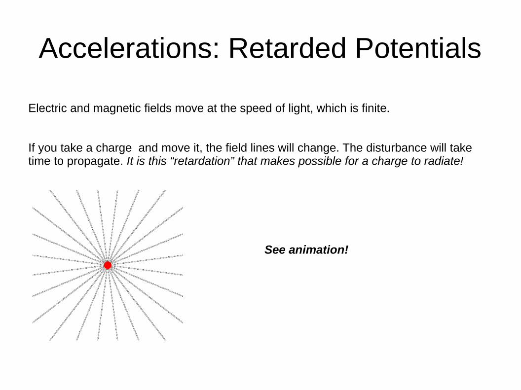
Accelerations: Retarded Potentials

Electric and magnetic fields move at the speed of light, which is finite.

If you take a charge and move it, the field lines will change. The disturbance will taketime to propagate. It is this “retardation” that makes possible for a charge to radiate!

See animation!

Velocity and Acceleration Fields

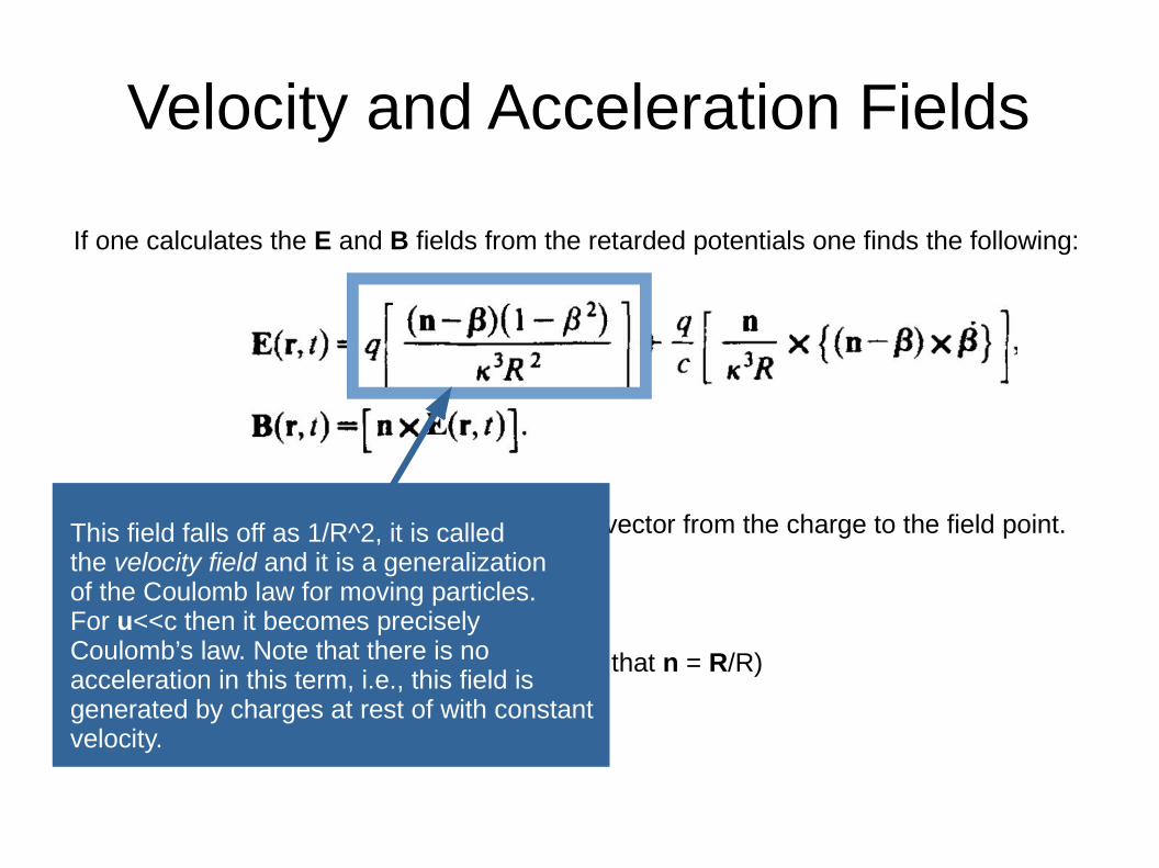
If one calculates the E and B fields from the retarded potentials one finds the following:

Here u is the velocity of the charge, n is a unit vector from the charge to the field point.

We have aso used the notation R = |r-r’| (so that n = R/R)

Velocity and Acceleration Fields

If one calculates the E and B fields from the retarded potentials one finds the following:

Here u is the velocity of the charge, n is a unit vector from the charge to the field point.

We have aso used the notation R = |r-r’| (so that n = R/R)

This field falls off as 1/R^2, it is calledthe velocity field and it is a generalizationof the Coulomb law for moving particles. For u<<c then it becomes precisely Coulomb’s law. Note that there is no acceleration in this term, i.e., this field isgenerated by charges at rest of with constantvelocity.

Velocity and Acceleration Fields

If one calculates the E and B fields from the retarded potentials one finds the following:

Here u is the velocity of the charge, n is a unit vector from the charge to the field point.

We have aso used the notation R = |r-r’| (so that n = R/R)

This field falls off as 1/R^2, it is calledthe velocity field and it is a generalizationof the Coulomb law for moving particles. For u<<c then it becomes precisely Coulomb’s law. Note that there is no acceleration in this term, i.e., this field isgenerated by charges at rest of with constantvelocity.

When u~c then the term k becomes very important and concentrates the fieldsin a narrow cone (beaming effect, see previous lecture).

Velocity and Acceleration Fields

If one calculates the E and B fields from the retarded potentials one finds the following:

Here u is the velocity of the charge, n is a unit vector from the charge to the field point.

We have aso used the notation R = |r-r’| (so that n = R/R)

This is the acceleration field, i.e., it appears when the charges are accelerated. Note that it falls off as 1/R, not as 1/R^2. The acceleration field is also known as the radiation field and it is orthogonal to n.

Larmor’s Formula

What can we say about the radiation field when the velocity is <<c? (non-relativistic case)

In this case beta<<1 and thus we can simplify the electric and magnetic field expressionsand obtain:

What is the Poynting vector S? (remember that the Poyinting vector defines the directiontowards which the energy carried by the em fields is directed. Here S is parallel to n; S has units of erg/s/cm^2, i.e., energy flux).

Since:

The Poynting vector has magnitude:

Larmor’s Formula

Note the angle theta!

The energy of the em. field is not isotropic butthere is a sin^2 !!

Larmor’s Formula

Now let’s calculate the power in a unit solid angle about n. To do this we multiply the Poynting vector (units: erg/s/cm^2) by an area dA (cm^2) to get a power (erg/s). How do we choose dA? We know that the solid angle dOmega = dA/R^2. Therefore:

And now we integrate the above expression over the whole solid angle Omega=4*piand we obtain the total power emitted by an accelerated charge in the non-relativisticapproximation:

Larmor’s Formula

IMPORTANT: The power emitted is proportional to the square of the charge and thesquare of the acceleration.

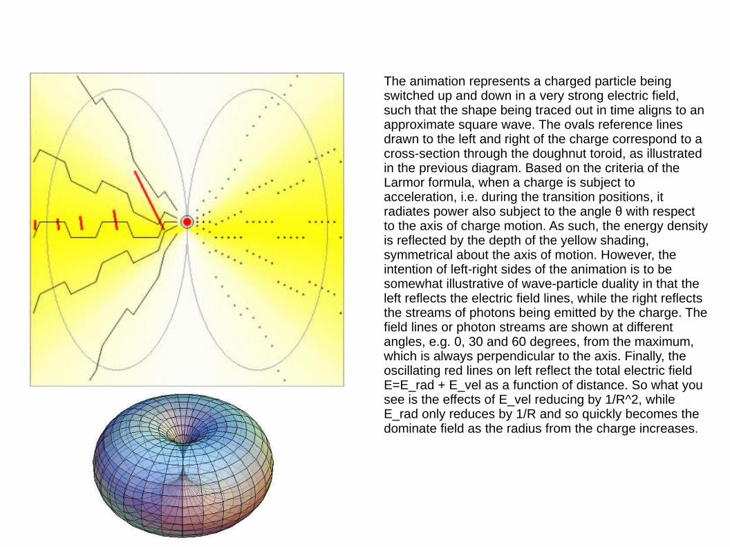
The animation represents a charged particle being switched up and down in a very strong electric field, such that the shape being traced out in time aligns to an approximate square wave. The ovals reference lines drawn to the left and right of the charge correspond to a cross-section through the doughnut toroid, as illustrated in the previous diagram. Based on the criteria of the Larmor formula, when a charge is subject to acceleration, i.e. during the transition positions, it radiates power also subject to the angle θ with respect to the axis of charge motion. As such, the energy density is reflected by the depth of the yellow shading, symmetrical about the axis of motion. However, the intention of left-right sides of the animation is to be somewhat illustrative of wave-particle duality in that the left reflects the electric field lines, while the right reflects the streams of photons being emitted by the charge. The field lines or photon streams are shown at different angles, e.g. 0, 30 and 60 degrees, from the maximum, which is always perpendicular to the axis. Finally, the oscillating red lines on left reflect the total electric field E=E_rad + E_vel as a function of distance. So what you see is the effects of E_vel reducing by 1/R^2, while E_rad only reduces by 1/R and so quickly becomes the dominate field as the radius from the charge increases.

Ensemble of Particles

So far so good, but what about an ensemble of particles? After all if we want to calculatethe properties of Bremsstrahlung radiation we need to consider a lot of particles...

Abell 1689 (z=0.18, i.e., about 2 billion light years away)

There is a complication here, because the expressions for the radiation fields refer to conditions at retarded times, and these retarded times will differ for each particleand we have an enormous amount of particles...

Solution: Let the typical size of the system be L, and let the typical time scale for changes within the system be T. If T is much longer than the time it takes light to travel a distance L, T>>L/c, then the differences inretarded time across the source are negligible.

Does this happen for example in an intracluster plasma?

Ensemble of Particles

Solution: call L the size of our cluster.Call R0 the distance from some point in the system to the field point (i.e., where we aresince we are measuring this field).But now you see that the difference between each Ri tends to zero as R0 → infinity (sincewe are very far away from the cluster!). So we can write:

Now our radiation field is:

Of course we have no idea what are the singlevelocities of each particle, neither we know howmany particles there are!

where is the dipole moment of the charges.

Dipole Approximation

Following the same procedure as for the single particle case, we can find the total poweremitted by an ensemble of particles (in the non-relativistic limit) in the so-called dipole approximation:

Now we have the key to understand Bremsstrahlung radiation...

Using Fourier transform we can easily find that:

Dipole Approximation

Following the same procedure as for the single particle case, we can find the total poweremitted by an ensemble of particles (in the non-relativistic limit) in the so-called dipole approximation:

Now we have the key to understand Bremsstrahlung radiation...

Using Fourier transform we can easily find that:

Remember how the Fourier Transform of a derivative works:

Dipole Approximation

Following the same procedure as for the single particle case, we can find the total poweremitted by an ensemble of particles (in the non-relativistic limit) in the so-called dipole approximation:

Now we have the key to understand Bremsstrahlung radiation...

Using Fourier transform we can easily find that:

This term instead comes from:

Dipole Approximation

Following the same procedure as for the single particle case, we can find the total poweremitted by an ensemble of particles (in the non-relativistic limit) in the so-called dipole approximation:

Now we have the key to understand Bremsstrahlung radiation...

Using Fourier transform we can easily find that:

This comes from Parseval’s Theorem.

Total energy per unit area in a pulse:

Small-Angle Scattering

To derive the properties of Bremsstrahlung radiation we will use an approximation calledsmall-angle scattering. This is an approximation in which the electron deflected by an ion deviates only by a small angle (typically <10 degrees).

Small angle scatteringSmall angle scattering NOT VALID

This approximation is not necessary but it simplifies the calculations and gives the rightequations.

Small Angle Scattering

b is the impact parameter (i.e., the perpendicular distance between the path of the electron and the ion of charge Ze). R is the actual distance between the electron and the ion. v is the speed of the electron. The dipole moment d=-eR. Therefore its second derivative is:

Small Angle ScatteringNow let’s take the Fourier transform of the second derivative of the dipole moment. This is:

(Remember that )

From the dipole approximation we know that the total energy emitted per unit frequency is:

So we need to solve the Fourier transform above andwe will know what is the energy emitted per unit frequency.

The electron interacts with the ion only for a small amount of time of the order of:

(collision time)

Therefore we can write:

Small Angle ScatteringNow let’s take the Fourier transform of the second derivative of the dipole moment. This is:

(Remember that )

From the dipole approximation we know that the total energy emitted per unit frequency is:

So we need to solve the Fourier transform above andwe will know what is the energy emitted per unit frequency.

The electron interacts with the ion only for a small amount of time of the order of:

(collision time)

Therefore we can write: (the exponential is unity)

(the exponential is zero)

Small Angle Scattering

So the energy emitted per unit frequency depends on the change of the electron velocityduring the collision time.

Now, we have an energy per unit frequency. But what we really want is the radiated powerper unit volume per unit frequency. Remember that for an isotropic emitter:

So we want to find here the energy per unit time per unit volume per unit frequency as well.

where P_nu was the power (i.e., energy per unit time) per unit volume per unit frequency.

dWd ω

→dW

d ωdV dtHow do we do this last step?

First we calculate how much has the speed changed ( ) , so we know Δ v

The acceleration (change in velocity) is given by the Coulomb force:

v=Fm

=Ze2

m b2 where I have used the fact that the interaction occurs at R~b only.

Then we multiply this acceleration by the collision time and we find Δ v

Δ v≈ v τ=vbv=

Z e2

m b v

Therefore depends on the impact parameter b, i.e., it is

dWd ω

→d W (b)

d ω∝

Z2 e6

m2 v2b2

Spectrum of an ensemble of particles with a single velocity v

dWd ωdV dtTo find the spectrum of an ensemble of particles with a single velocity v

we need to first integrate over the impact parameter b, then divide by the unit volume and time.

Now, say that the plasma has a certain electron density ne and ion density ni, and that all the electrons have the same speed v. The area around each ion that is importantfor the interaction is:

dWd ωdV dt

=ne ni 2π v∫bmin

∞ dW (b)

d ωb dbdA=2π b db

(units of 1/volume)

Spectrum of an ensemble of particles with a single velocity v

Now the treatment on how to choose the boundaries of the integration becomes quitelengthy and complicated. We are interested only in a few features that will determinehow the final spectrum will look like.

The final spectrum of plasma with electron having a single velocity v will look like the following:

The Gaunt factor contains quantum corrections which we have not taken properly intoaccount here, but can be approximated as:

( Pν=jν

4 π=

dWd νdV dt )

Thermal Bremsstrahlung

How do we go from the spectrum of an ensemble of ions and electrons (with the latter all havinga single velocity v) to the spectrum of an ensemble of ions and electrons with a distributionof velocities?

First we need to know which distribution of velocities.

Let’s take the most common case (almost always the case in astrophysics) which is that of a thermal plasma, i.e., electrons and ions with velocities distributed according to the Maxwell-Boltzmann distribution (see also Lecture 3!).

F (v)dv=4π v2 ( m2π k T )

3 / 2

e−mv2 / 2kT dv

We then need to integrate over this distribution

From Lecture3: Matter in Thermal Equilibrium

Suppose to have a plasma in thermal equilibrium (thermal plasma). What does this mean in terms of micro-physical properties of the matter?

F( v)dv=4 π v2 ( m2π kT )

3 / 2

e−mv2 / 2kT dv

Probability distribution function of (non-relativistic) velocities is the Maxwell-Boltzmann distribution:

Spectrum:Thermal Bremsstrahlung

Why there is a minimum velocity in the integral? Shouldn’t we use zero as the minimum?

Spectrum:Thermal Bremsstrahlung

Why there is a minimum velocity in the integral? Shouldn’t we use zero as the minimum?

The photons need to be created during the deceleration of the electron. So the initial kinetic energy of the electron must be larger than the photon energy. This creates a cutoff in the spectrum and this is due to the discreteness of photons, i.e., theyare discrete and not continuum entities.

vmin=(2h ν/m)1/2

Spectrum:Thermal Bremsstrahlung

Performing the integration one gets:

ενff=

dWd νdV dt

BE CAREFUL do NOT make a confusion between and defined as the emissivity at page 9. Also, R&L uses the same symbol to define the probability of absorption at page 37.

Furthermore the difference between and is the following:

→ (energy/frequency/volume/time).

ενff ϵν

ϵν

jν

jν → (energy/frequency/volume/time/solid angle).

ενff

ενff

Also, the symbol is exactly the same as in ενff Pν

The reason why R&L uses different symbols here is correct: will refer from now on onlyto Bremsstrahlung. The symbol is a general one and it equal to only for Bremsstrahlung

ενff

Pν ενff

Spectrum:Thermal BremsstrahlungPerforming the integration one gets:

What do we see here? The emission coefficient seem to depend on the temperature (be careful because T is alsoin the exponential), on the density of ions and electrons and on the ion charge. The frequency dependency is only in the exponential. The average Gaunt factor can be considered very close to unity since this is its order of magnitude.

ενff=

dWd νdV dt

Also, the spectrum will be basically flat, except when exp(-h*nu/kT) becomes dominant. This happens when the thermal energy of electronsis basically insufficient to generate high energy photons.

ε νff=

dWdν

dVdt

Thermal Bremsstrahlung: Absorption

If we have thermal emission then we can always use Kirchhoff’s law.

What happens at low frequencies?

Thermal Bremsstrahlung: Absorption

If we have thermal emission then we can always use Kirchhoff’s law.

ενff=

dWd νdV dt

=4 π jνff

We see that when we are in the Rayleigh-Jeans regime:

What happens at low frequencies?

This is telling us that the spectrum of Bremsstrahlung is self-absorbed at low frequencies.Why?

Thermal Bremsstrahlung

Remember that the optical depth is defined as: d τν=αν ds

Therefore since we have that as well. τν∝ν−2

The smaller the frequencies, the larger the optical depth. This means that radiation is absorbed more and more before leaving the system. But this is precisely whata blackbody is! So at low frequencies we expect a blackbody like spectrum.

So what is the specific brightness of Bremsstrahlungradiation?

At low frequency we expect it to look like blackbody.At intermediate frequencies it has to be flatAt high frequencies there must be an exponential cutoff

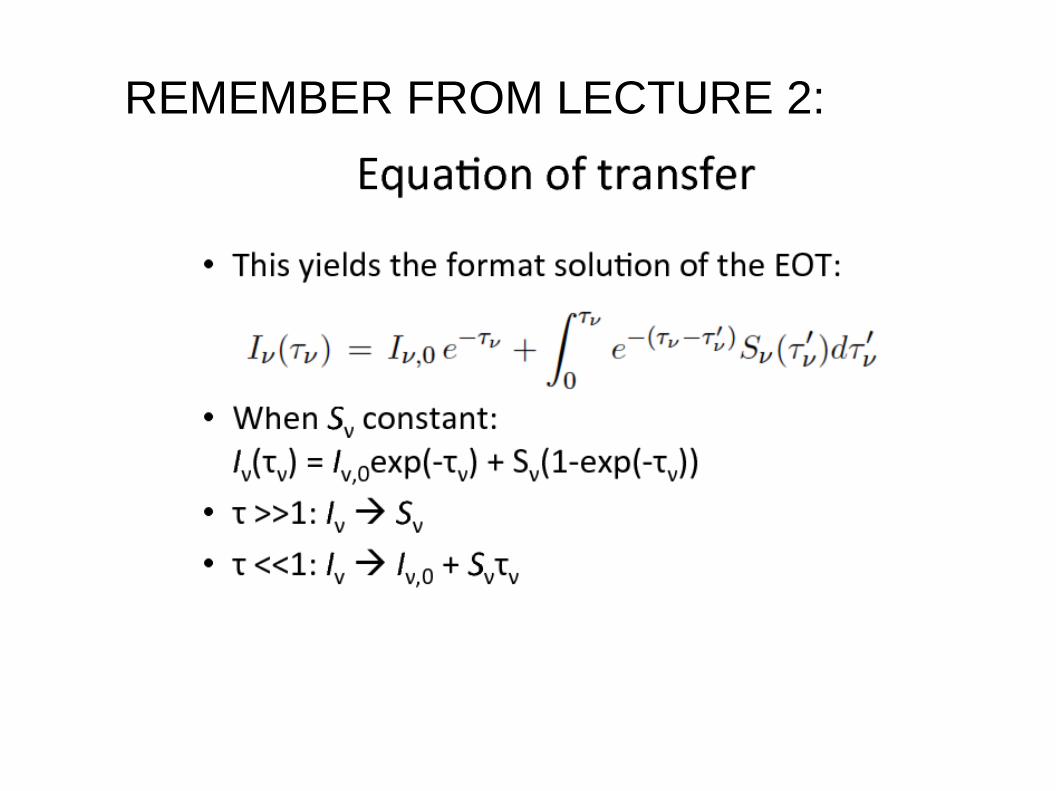
REMEMBER FROM LECTURE 2:

REMEMBER FROM LECTURE 2:

REMEMBER FROM LECTURE 2:

.=εν

ff R4 π

.=jναν

=Sν=Bν

Thermal BremsstrahlungNow we can understand the spectrum of Bremsstrahlung!

At large optical depths: Blackbody

At small optical depths:

ενff=

dWd νdV dt

=4 π jνff

If the region of size R has large optical depth at any frequency then Bremsstrahlung becomesBlackbody spectrum (solid line). Otherwise is will show the typical flat spectrum in the intermediate frequencies, blackbody spectrum at low frequencies at cutoff at high frequencies

Cooling Time

Since we know how much does a thin plasma radiate we can calculate the energy lossesand the so-called cooling time:

energy content of the plasma

rate of energy loss

32(ne+ni)k T

εff =

3 nkTε

ff=

Here we have integrated the emission coefficient over all frequencies:ενff

τcool=6×103 T 1/2 ne−1 g ff yr

L=εff V

This is useful to calculate the cooling time:

Cooling Time: HII regions

The Orion nebula is an HII region. Here you see the radio continuum overlaid to the optical image. The radio continuum isBremsstrahlung emission.

τcool=6×103 T 1/2 ne−1 gff yr

What is the cooling time of the nebula?

Here ne ~ 100-1000 cm^-3T ~ 10,000 K

The cooling time is of the order of a fewthousands years.

But the nebula has an age of 3 Myr. So what does this mean?

Cooling Time: Intracluster medium

Here the typical temperatures are 10^7 K (indeed wesee most radiation in X-rays, whereas in the Orion nebula it was mostly at radio waves).The typical densities are also very low:

ne~0.001 cm^-3

τcool=6×103 T 1/2 ne−1 g ff yr≈10 Gyr

Intracluster gas takes a very long time to cool down!

Thermal Blackbody Bremsstrahlung Synchrotron Inverse Compton

Optically thick – YES NO

Maxwellian distributionof velocities

YES YES –

Relativistic speeds

– – –

Main Properties Matter in thermal equilibrium

Matter AND radiation in thermal equilibrium

Radiation emitted by accelerating particles

Summary of Radiation Properties

Rules of thumb: 1. Blackbody is always thermal, but thermal radiation is not always blackbody (e.g., thermal Bremsstrahlung)2. Bremsstrahlung can be thermal or non-thermal. 3. Bremsstrahlung becomes blackbody when optical depth >>1.