Bridge Performance and Design

Bridge Performance & Design LDA0901

Worcester Polytechnic Institute Major Qualifying Project C09

1

Bridge Performance and Design

A Major Qualifying Project Report

Submitted to the Faculty of

The Worcester Polytechnic Institute

In Partial Fulfillment of the Requirements for the Degree of Bachelor of Science

Prepared by:

Alejandro Sosa-Boyd Sezai Emre Gazioglu

Douglas Heath Daniel White

Besian Xhixho

Submitted to: Professor Leonard Albano, Project Advisor

2009



2

Abstract

This project studied the structural design of a highway bridge superstructure and

substructure. The results were used to develop initial and life-cycle cost estimates. Guidelines

are established for young engineers to follow in a preliminary design of these components.

Finite element models were developed to study the distribution of loads through superstructures,

and stress distributions in bridge connections. Simplified modeling techniques are presented,

and provide a basis for capturing the stiffness provided by bracing members in analytical models.



3

Authorship

All members of the project group made an equal contribution to this project. All

members were involved in the development of project objectives, and played a role in the final

assembly of the project report. Chapter I (Introduction), Chapter II (Background), Chapter III

(Methodology), and Chapter IX (Conclusions) were written by all group members. Primary

authors for the remaining chapters are as follows:

Chapter IV (Superstructure): Sezai Emre Gazioglu & Douglas Heath

Chapter V (Substructure): Alejandro Sosa Boyd & Daniel White

Chapter VI (Life-Cycle Cost Analysis of Bearings): Besian Xhixho

Chapter VII (Effect of Bracing on Lateral Load Distribution): Douglas Heath

Chapter VIII (Finite Element of Clip Angle Connection): Besian Xhixho

________________________________ ________________________________

Sezai Emre Gazioglu Alejandro Sosa Boyd

________________________________ ________________________________

Douglas Heath Daniel White

________________________________

Besian Xhixho



4

Capstone Design

This project considered many of the real world constraints provided by ASCE to fulfill

the capstone design requirement. The following list identifies the five constraints considered in

this project, and how each one was addressed:

Economic: Several superstructure design options were established and designed; cost analyses

were conducted on all designs. The initial construction cost of the designs were compared, and

the least expensive option was identified.

Sustainability: Life cycle cost analyses were conducted for the substructure design and bearing

type selection. These analyses provided a way for designing a system that will minimize

maintenance/additional investment over the life of the structure.

Constructability: Constructability was considered throughout the project. The designs provided

consist of standard steel shapes or shapes with regular dimensions (dimensions rounded to the

nearest whole number). Also, the constructability of large concrete sections is discussed in

Chapter IV.

Ethical: This project considered ethical constraints by identifying potential problems with

designs. For example, in Chapter IV, several design alternatives are proposed, however,

problems related to cracking of concrete are identified. It is important for engineers to ensure

that the limitations and potential problems associated with their designs are clear to the owner.

Health and Safety: These constraints were addressed by basing the designs on the AASHTO

bridge design specification. Adhering to this specification provides a reasonable level of

confidence that the structure will be structurally sound, and not pose a high level of risk to

human life.



5

Table of Contents

I INTRODUCTION ........................................................................................................................................ 15

II BACKGROUND .......................................................................................................................................... 17

II.1 THE SUPERSTRUCTURE .................................................................................................................................... 17

II.1.1 The Deck & Girders .............................................................................................................................. 18

II.1.2 Bracing Members ................................................................................................................................. 19

II.2 SUBSTRUCTURE ............................................................................................................................................. 20

II.2.1 Bearings ............................................................................................................................................... 20

II.2.2 Piers ..................................................................................................................................................... 21

II.2.3 Abutments and Retaining Structures ................................................................................................... 23

II.2.4 Foundations ......................................................................................................................................... 25

II.3 DESIGN LOADS .............................................................................................................................................. 27

II.4 LIFE-CYCLE COST ANALYSIS .............................................................................................................................. 27

II.5 FINITE ELEMENT ANALYSIS ............................................................................................................................... 28

II.6 REMARKS ..................................................................................................................................................... 29

III METHODOLOGY ....................................................................................................................................... 31

IV SUPERSTRUCTURE DESIGN ....................................................................................................................... 34

IV.1 DESIGN METHODOLOGY ................................................................................................................................. 34

IV.1.1 Deck Design .......................................................................................................................................... 41

IV.1.2 Girder Design ....................................................................................................................................... 43

IV.1.3 Cost Estimate ....................................................................................................................................... 48

IV.2 DESIGN RESULTS ............................................................................................................................................ 49

IV.2.1 Option 1 Design Results ....................................................................................................................... 49




6


IV.2.3 Cost Analysis Results ............................................................................................................................ 63

IV.2.4 Investigate Advantages of Continuous Span Girders ............................................................................ 65

IV.2.5 Investigate Advantages of Composite Sections .................................................................................... 66

IV.2.6 Investigate the Economy of Different Building Materials ..................................................................... 66

IV.2.7 Investigate the Effect of the Deck Spanning Transversely vs. Longitudinally ....................................... 68

IV.2.8 Investigate the Effect of Having an Overhang ...................................................................................... 69

IV.3 REMARKS ..................................................................................................................................................... 70

V SUBSTRUCTURE DESIGN ........................................................................................................................... 72

V.1 PIER DESIGN ................................................................................................................................................. 72

V.1.1 Design Background .............................................................................................................................. 72

V.1.2 Design Methodology ............................................................................................................................ 75

V.1.3 Pier Foundation Design Methodology .................................................................................................. 79

V.1.4 Design Results ...................................................................................................................................... 81

V.1.5 Life-Cycle Cost Analysis ........................................................................................................................ 86

V.1.6 Remarks ............................................................................................................................................... 89

V.2 ABUTMENT DESIGN ....................................................................................................................................... 90

V.2.1 Design Background .............................................................................................................................. 90

V.2.2 Design Methodology ............................................................................................................................ 92

V.2.3 Abutment Foundation Design Methodology ........................................................................................ 97

V.2.4 Abutment Design Results ..................................................................................................................... 97

V.2.5 Abutment Life-Cycle Cost Analysis ..................................................................................................... 101

V.2.6 Remarks ............................................................................................................................................. 104

VI LIFE CYCLE COST ANALYSIS OF BEARINGS ................................................................................................ 105

VI.1 METHODOLOGY .......................................................................................................................................... 105



7

VI.2 RESULTS ..................................................................................................................................................... 108

VI.3 CONCLUSIONS ............................................................................................................................................. 120

VII EFFECT OF BRACING ON LATERAL LOAD DISTRIBUTION ........................................................................... 123

VII.1 DEVELOPMENT OF A SIMPLIFIED FINITE ELEMENT MODEL .................................................................................... 123

VII.1.1 Simplified Model Literature Review ............................................................................................... 124

VII.1.2 Development of the Model ............................................................................................................ 127

VII.1.2.1 Validating the Model ................................................................................................................................ 132

VII.2 MOMENT DISTRIBUTION FACTORS .................................................................................................................. 133

VII.2.1 Background ................................................................................................................................... 134

VII.2.2 Moment Distribution Results ....................................................................................................... 137

VII.3 SHEAR LAG AND EFFECTIVE WIDTH ................................................................................................................. 140

VII.3.1 Background on Shear Lag and Effective Width ............................................................................. 141

VII.3.2 Results of Shear Lag Investigation ............................................................................................... 144

VII.4 REMARKS ................................................................................................................................................... 149

VIII FINITE ELEMENT ANALYSIS OF CLIP ANGLE CONNECTIONS .................................................................. 151

VIII.1 METHODOLOGY .......................................................................................................................................... 152

VIII.2 RESULTS ..................................................................................................................................................... 159

VIII.3 CONCLUSIONS ............................................................................................................................................. 171

IX CONCLUSIONS ........................................................................................................................................ 175

IX.1 BRIDGE DECK .............................................................................................................................................. 177

IX.2 BRACING MEMBERS ..................................................................................................................................... 177

IX.3 CONNECTIONS ............................................................................................................................................ 178

IX.4 GIRDERS .................................................................................................................................................... 178

IX.5 BEARINGS .................................................................................................................................................. 179



8

IX.6 PIERS ........................................................................................................................................................ 180

IX.7 ABUTMENTS ............................................................................................................................................... 181

IX.8 FOUNDATIONS ............................................................................................................................................ 181

IX.9 FINAL REMARKS .......................................................................................................................................... 182

WORKS CITED ................................................................................................................................................. 184

Appendix



9

Table of Figures

Figure 1: Bridge Components ....................................................................................................... 18

Figure 2: Typical Pier Types for Steel Bridges ............................................................................. 22

Figure 3: Typical Pier Types for Concrete Bridges ....................................................................... 22

Figure 4: Typical Abutment Types ................................................................................................ 24

Figure 5: Shallow Foundations ..................................................................................................... 25

Figure 6: Deep Foundations .......................................................................................................... 26

Figure 7: Plan of Highway to be Crossed ..................................................................................... 35

Figure 8: Bridge Elevation View .................................................................................................. 36

Figure 9: Plan View of Bridge at Top of Deck .............................................................................. 37

Figure 10: Design Option 1........................................................................................................... 37

Figure 11: Design Option 2 ........................................................................................................... 38

Figure 12: Design Option 3........................................................................................................... 39

Figure 13: AASHTO Design Truck .............................................................................................. 42

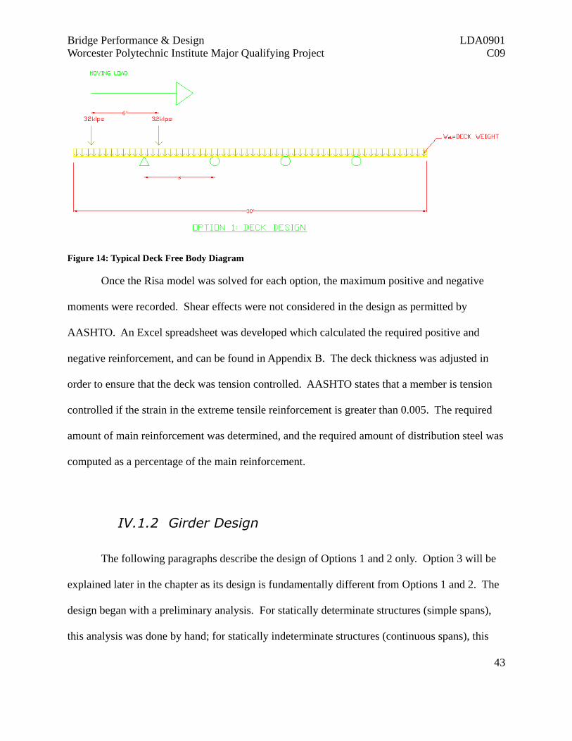
Figure 14: Typical Deck Free Body Diagram ............................................................................... 43

Figure 15: Typical Free Body Diagram for Girder Design ........................................................... 44

Figure 16: Steel Girder Design Procedure .................................................................................... 45

Figure 17: Concrete Girder Design Procedure .............................................................................. 46

Figure 18: Option 3 Free Body Diagrams ..................................................................................... 48

Figure 19: Option 1 Concrete Design Results .............................................................................. 50

Figure 20: Option 1 Steel Design Results ..................................................................................... 51

Figure 21: Option 1 Steel Design Results (continued) ................................................................. 52



10

Figure 22: Option 1 Overhang Alternative 1 ................................................................................ 53

Figure 23: Braced Design Alternative ........................................................................................... 54

Figure 24: Horizontal Bracing for Deck Alternative 2 ................................................................. 55

Figure 25: Option 2 Concrete Design Results .............................................................................. 56


Figure 27: Option 2 Steel Design Results (continued) ................................................................. 59

Figure 28: Option 3 Concrete Design Layout ............................................................................... 60


Figure 30: Pier Design Sketch ...................................................................................................... 74

Figure 31: Cap Design Flow Chart ............................................................................................... 77

Figure 32: Column Design Flow Chart ......................................................................................... 78

Figure 33: Footing Design Flow Chart ......................................................................................... 78

Figure 34: Deep Foundation Design Flow Chart .......................................................................... 80

Figure 35: Layout of Piles of the Deep Foundation for the Single Leg Pier ................................ 81

Figure 36: Multi-Column Pier Cap Cross-Section with Reinforcement ....................................... 83

Figure 37: Multi-Column Pier Column Cross-Section with Reinforcement ................................ 83

Figure 38: Multi-Column Pier Footing Cross-Section with Reinforcement ................................. 84

Figure 39: Single Leg Pier Cap Cross-Section with Reinforcement ............................................ 84

Figure 40: Single Leg Pier Column Cross-Section with Reinforcement ...................................... 84

Figure 41: Single Leg Pier Footing Cross-Section with Reinforcement ...................................... 85

Figure 42: Typical Abutment Types. ............................................................................................. 91

Figure 43: Abutment Size Specifications (McCormac) ................................................................ 93

Figure 44: Final Abutment Sizes................................................................................................... 94



11

Figure 45: Backwall & Stem Design Procedure ........................................................................... 95

Figure 46: Footing Design Procedure ........................................................................................... 96

Figure 47: Loads Acting on the Abutment .................................................................................... 97

Figure 48: Abutment Reinforcements ........................................................................................... 98

Figure 49: Abutment Stem With Reinforcement .......................................................................... 99

Figure 50: Abutment Backwall with Reinforcement .................................................................. 100

Figure 51: Abutment Footing with Reinforcement ..................................................................... 101

Figure 52: Superimposed Results ............................................................................................... 118

Figure 53: Process of Attaining Absolute Cost ........................................................................... 119

Figure 54: Process of Obtaining Labor Costs ............................................................................. 119

Figure 55: Simplified FEM G1 Diagram .................................................................................... 125

Figure 56: Superstructure Finite Element Model ........................................................................ 128

Figure 57: Simplified FEM Components .................................................................................... 129

Figure 58: Live Load Location ................................................................................................... 130

Figure 59: Bracing Types Investigated ....................................................................................... 131

Figure 60: Horizontal Bracing Plan ............................................................................................ 132

Figure 61: Shear Lag in Composite Sections .............................................................................. 142

Figure 62: Longitudinal Stress Distribution vs. Transverse Deck Location (no bracing &

horizontal bracing) ...................................................................................................................... 145

Figure 63: Longitudinal Stress Distribution vs. Transverse Deck Location (horizontal bracing

present) ........................................................................................................................................ 146

Figure 64: Longitudinal Stress Distribution vs. Transverse Deck Location (no horizontal bracing)

..................................................................................................................................................... 147



12

Figure 65: Percent Change in Stress Intensity (horizontal bracing present) ............................... 148

Figure 66: Percent Change in Stress Intensity (no horizontal bracing) ...................................... 148

Figure 67: Finite Element Model for the Entire Mesh ................................................................ 155

Figure 68: Finite Element Model for the Connection Details ..................................................... 156

Figure 69: Model 1; Stress Distribution in Entire Model ........................................................... 160

Figure 70: Model 1; Stress Distribution on Clip Angle (Regular Plot Scale) ............................. 161

Figure 71: Model 1; Stress Distribution on Clip Angle (modified plot scale) ............................ 162

Figure 72: Model 1; Clip Angle's Surface Attached to the Web of the Floor Beam ................... 163

Figure 73: Model 2; Stress Distribution on Clip Angle (regular plot scale) ............................... 164



Figure 76: Model 3...................................................................................................................... 167



Figure 79: Distribution of Principal Stress from Analysis using Fixed Rotation Model of Floor

Beam ........................................................................................................................................... 170

Figure 80: Distribution of Principal Stress from Analysis using Fixed Top Flange Model of Floor

Beam ........................................................................................................................................... 171

Figure 81: Bridge Load Path Summary ...................................................................................... 176



13

Table of Tables

Table 1: Design Option Summary ................................................................................................. 40

Table 2: Sample Cost Estimate Sheet ........................................................................................... 49

Table 3: Option 3 Concrete Design Results .................................................................................. 61

Table 4: Cost Analysis Summary .................................................................................................. 64

Table 5: Limit states of different pier components ....................................................................... 73

Table 6: Assumed soil conditions for pier foundation design ....................................................... 79

Table 7: Pier design reinforcement results .................................................................................... 82

Table 8: Pier foundation results .................................................................................................... 85

Table 9: Costs of pier components (Ito, 2009) .............................................................................. 87

Table 10: Material quantities used in pier designs ........................................................................ 87

Table 11: Results of the life-cycle cost analyses ........................................................................... 89

Table 12: Cost of Materials and Maintenance ............................................................................ 102

Table 13: Abutment Steel Reinforcement by Weight .................................................................. 102

Table 14: Abutment Steel Reinforcement Cost by Volume ........................................................ 102

Table 15: Abutment Concrete Cost by Volume ........................................................................... 103

Table 16: Repair Cost of Abutment ............................................................................................ 103

Table 17: Life-Cycle Cost Analysis Results ............................................................................... 103

Table 18: Cost Data ..................................................................................................................... 109

Table 19: Cost Data ..................................................................................................................... 109

Table 20: Cost Data ..................................................................................................................... 110

Table 21: Absolute Low, Average and High Estimates ............................................................... 112



14

Table 22: Low Economic Life .................................................................................................... 112

Table 23: Average Economic Life ............................................................................................... 113

Table 24: High Economic Life .................................................................................................... 113

Table 25: Results ......................................................................................................................... 114

Table 26: High Labor Costs ........................................................................................................ 114

Table 27: Low Economic Life .................................................................................................... 115

Table 28: Average Economic Life ............................................................................................... 116

Table 29: High Economic Life .................................................................................................... 116

Table 30: Results ......................................................................................................................... 117

Table 31: Simplified FEM Summary .......................................................................................... 127

Table 32: Model Summary .......................................................................................................... 128

Table 33: Comparison of AASHTO MDF to MDF Predicted by ANSYS ................................. 137

Table 34: Comparison of MDF by Bracing Type........................................................................ 138

Table 35: Comparison of MDF by Bracing Stiffness .................................................................. 140

Table 36: Summary of Relevant Design Parameters .................................................................. 153

Table 37: Analysis and Contact Parameters ................................................................................ 158

Table 38: Clip Angle Thickness Capacity ................................................................................... 159



15

I Introduction

Bridges are important structures in any society; they are especially important to trade by

providing a time efficient means of crossing an obstacle. For example, suppose that the only

factory in the country that manufactures toothbrushes were located on an island. The only way

to get the toothbrushes off of the island and into stores where they could be sold would be to load

the toothbrushes onto a ship or airplane that could take them to the mainland, or to build a bridge

and transport them by truck. It is likely that the most cost-effective and time efficient option

would be to transport the items by truck (neglecting the cost and construction time required to

build the actual bridge). This concept of developing a time and cost efficient method of

distributing goods is applicable to most of the products purchased today, and the financial

savings that distributor generate by means of the bridge gives the structure value. Also, bridges

allow easy travel within a region by providing a means to cross a river or gorge, for example.

The service provided by bridges to travelers adds even more value to the bridge. The value

added to the bridge by the savings of product distributors and travelers makes it a cost-effective

and important piece of infrastructure for trade and travel.

As was highlighted in the previous paragraph, bridges are very important structures to a

society. Because of this, it is important that they are structurally sound, and that they do not

collapse or go out of service for any other reason. This would not only threaten human life due

to the danger associated with a collapse, but it would also have severe financial implications,

both in terms of the investment in the bridge itself and the loss of an important travel route to

product distributors and travelers. To assure the quality of bridges, engineers have studied their

behavior, and developed guidelines for designing and constructing them in a structurally sound



16

manner. These guidelines have been made available by the American Association of State

Highway and Transportation Officials (AASHTO).

This project studied the basic design of a bridge, particularly a highway overpass. This

type of bridge is one of the simplest to design and was a good starting point for a young bridge

engineer. The guidelines published by AASHTO were consulted to design various key

components of the bridge, such as substructure elements (piers, abutments, and foundations) and

superstructure elements (bridge deck, girders, and bracing members). In addition to studying the

design of these basic structural components, this project also pursued several topics in depth.

These topics included a life-cycle cost analysis of bridge bearings, an analysis of the effect of

bracing on laterally distributing deck loads, and an analysis of a typical bridge connection. The

project team was able to synthesize the results of all the designs and investigations conducted in

the project, and develop an understanding of how bridges behave and how a structural design can

affect project constraints (cost, constructability, etc.)

Consulting the AASHTO guidelines for the design of basic bridge components provided

the project team with experience in the design of the components, and caused the project team to

develop an appreciation for the guidelines published by engineering associations to protect life.

By designing basic bridge components, the project team was also required to consider the

constructability of a design. Finally, the cost analysis and life-cycle cost analysis activities

associated with this project increased the project team's understanding of the importance of cost;

not only the initial cost of construction, but also the cost of maintaining a bridge over its lifetime.

An understanding of these concepts is not only be valuable to bridge design and construction, but

to the design and construction of all structures.



17

II Background

To design a bridge, a fundamental understanding of its basic structural components and

how they behave when loaded is needed. First, different components that make up a bridge are

discussed; these are divided into two categories, superstructure components and substructure

components. The principles behind life-cycle cost analysis are then investigated. Finally, the

fundamental ideas behind finite element analyses are discussed, providing the reader with some

background in this powerful tool for analysis.

The Superstructure

To get a better understanding of the components of the bridge, it is divided into two

sections, the superstructure and the substructure. The superstructure is generally composed of the

deck, girders, and bracing. The superstructure carries the traffic loads on the bridge and transfers

them to the substructure. Figure 1, below, shows the different parts of the bridge. Items one and

two are part of the superstructure.



18

Figure 1: Bridge Components

Carmichael, Adam and Desrosiers Nathan. "Comparative Highway Bridge Design." 28 Feb. 2008. Worcester

Polytechnic Institute. 10 Sept. 08 http://www.wpi.edu/pubs/e-project/available/e-project-022608-

180459/unrestricted/comparative_highway_bridge_design_lda0802.pdf.

II.1.1 The Deck & Girders

The deck is the topmost part of the bridge, and is the part which comes into direct contact

with traffic. It is also referred to as the slab. The deck is generally made from concrete, which is

usually cast in place. The deck is supported by the girders, also known as stringers. The girders

carry the load from the deck, and transfer it to the substructure at the piers and abutments. The

girders are usually made from either reinforced concrete or steel.

In design, the spacing of the girders is often varied. This variation affects the size of the

http://www.wpi.edu/pubs/e-project/available/e-project-022608-180459/unrestricted/comparative_highway_bridge_design_lda0802.pdf




19

deck and the girders. The most economical spacing option based upon the total cost of the

girders and the deck is then chosen. When the spacing between girders becomes large,

intermediate beams are added to the structural system. These beams are placed perpendicular to

traffic, and they frame into the girders. This prevents a need for a large and heavily reinforced

deck (Xanthakos, 1994).

The deck can act compositely with the girders by connecting the elements together with

shear studs. This provides extra load carrying capacity to the system because the two members

work together to resist loads (Tonias, 1995). There are several design considerations associated

with composite deck-girder systems; one consideration is the effect of a change in curvature of

the system for continuous girders (Xanthakos, 1994). Despite the complexities associated with

the design of composite systems, the American Association of State Highway Transportation

Officials recommends their use unless it is prohibited by some factor (AASHTO, 2007).

II.1.2 Bracing Members

Bracing members are often used in girder bridges to help distribute loads. There are

many different types of bracing that can be used. Members can be placed between the girders in

an “X shape,” in which case the bracing acts like a truss to stiffen the superstructure. Beams are

sometimes used instead, and have a similar effect. AASHTO recommends the use of bracing

members to help resist wind load and limit lateral deflection. There is also research which

indicates that the use of bracing members may help to distribute the applied loads among more

girders, which would decrease the maximum girder moment. AASHTO recommends a

maximum bracing spacing of 25 feet (Eamon and Nowak, 2002).



20

Substructure

The substructure supports the superstructure. It carries the loads above it, and transfers

them to the foundations, and then to the ground. The substructure is made up of bearings, piers,

abutments, and foundations.

II.1.3 Bearings

Bearings connect the girders to the piers and abutments to transmit loads such as the

superstructure self-weight, traffic loads, wind loads, and earthquake loads from the

superstructure to the rest of the substructure. The bearings allow translational and rotational

movement in both the longitudinal and transverse directions. Translational movements are

caused by shrinkage, creep, and temperature effects, while rotation movements are caused by

traffic loads and uneven settlement of the foundations

Bearings can be classified as fixed bearings, allowing rotations but restricting

translational movements, or as expansion bearings, allowing both rotational and translational

movements. Sliding, roller, and elastomeric bearings fall into the expansion type, while rocker

and pin bearings in the fixed type. In contrast with other expansion bearings, roller and

elastomeric bearings are suitable for both steel and concrete girders. Roller bearings can be

composed of a single or multiple rollers. Single roller bearings have a low manufacturing cost

but at the same time have very little vertical load capacity; in contrast, multiple roller bearings

can support large loads but are more expensive. Elastomeric bearings are made of a natural or

synthetic rubber called elastomer. They accommodate translational and rotational movements by

the deformation of this rubber. Elastomeric bearings are the most common because they are



21

inexpensive and almost maintenance free, while still being tolerant with respect to loads and

movements greater than the design values (Chen & Duan, 1999).

II.1.4 Piers

In a basic sense, piers are elements that connect the superstructure to the ground at any

point that is not an end of the bridge. They are responsible for providing support for the girders

at intermediate points along the bridge, and transferring the load from the superstructure to the

foundations. Even though piers are commonly designed to resist vertical loads, design

precautions are taken to also resist lateral wind loads (Chen & Duan, 1999).

There are many different types of piers and the selection of a specific pier depends upon

what the bridge will be made out of and what it will be used for. The typical pier types for steel

bridges are hammerhead, solid wall, and rigid frame piers as shown in the following Figure 2.

For concrete bridges, the typical pier types are the bents, and can be designed for pre-cast girders

and for cast-in-place girders as shown in Figure 3. The type of pier differs depending upon the

material used for the girders because of the difference in the weights of the types of girders.

Bents can support more dead load from the superstructure than other types of piers.



22

Figure 2: Typical Pier Types for Steel Bridges

Chen, Wai-Fah (Ed.) & Duan, Lian (Ed.) (1999). Bridge Engineering Handbook. Boca Raton, Florida: CRC

Press

Figure 3: Typical Pier Types for Concrete Bridges


Press



23

II.1.5 Abutments and Retaining Structures

The same way piers provide vertical and lateral support at intermediate points in the

bridge superstructure; abutments and retaining structures provide vertical and lateral support at

the bridge‟s ends. In addition, abutments serve as connections between the bridge and the

approach roadway, while retaining the roadway materials from the bridge span (Chen & Duan,

1999).

A bridge abutment can be classified as either open-end or closed-end depending on its

relation with the roadway it passes over. Open-end abutment have slopes between the bridge

abutment face and the edge of the roadway or river canal that the bridge crosses over. Closed-

end abutment are high vertical walls that have no slope (Chen & Duan, 1999).

Abutments can also be classified according to the connections between the abutment stem

and the bridge superstructure, as monolithic or seat-type abutments (see figure below). The

monolithic abutment is built with the bridge superstructure; in contrast, the seat-type abutment is

built separately from the bridge superstructure. For monolithic abutments, there is no

displacement permitted between the superstructure and the abutment. This means that concrete

girders could be cast directly into the abutments. For the seat-type abutments, the superstructure

rests on the abutment stem through bearing pads, rock bearings, or other devices (Chen & Duan,

1999).



24

Figure 4: Typical Abutment Types


Press

The design of abutments depends in part upon the soil conditions at the project site. If the

site is mostly hard bedrock, a vertical, close-end, abutment will be sufficient. If the soil is softer,

a sloped, open-end, abutment will most likely be necessary to help counteract settlement.

However, the use of sloped abutments usually requires longer bridge spans and extra earthwork;

this could increase in the bridge construction cost (Chen & Duan, 1999).



25

II.1.6 Foundations

Foundations are structural elements that serve as a connection between the bridge

substructure and the ground. These structural elements can be classified as either shallow or

deep. Shallow foundations include spread footings, which are foundations that transmit the loads

to soil near the surface (Figure 5). Deep foundations include piles, drilled shafts, caissons,

anchors and others, which transmit all or some of the loads to deeper soils (Figure 6). (Coduto,

2001)

Figure 5: Shallow Foundations


Press



26

Figure 6: Deep Foundations

Chen, Wai-Fah (Ed.) & Duan, Lian (Ed.) (1999). Bridge Engineering Handbook. Boca Raton,

Florida: CRC Press

Shallow foundations are used in good soil conditions. They are able to transfer vertical

loads to the soil using bearing pressure. Deep foundations are used when the soil conditions near



27

the surface are poor and the bearing pressure is not sufficient to carry the load. In these cases the

foundation needs to extend to a deeper, solid layer of soil and take advantage of side friction in

order to transfer the loads.

Design Loads

AASHTO provides many different types of loads to be considered in bridge design.

These loads can be classified in one of two categories: permanent (dead) loads and temporary

(live) loads. Permanent loads are generally fairly easy to determine because the unit weights of

commonly used materials are provided in relevant bridge design codes. Live loads can be

broken down into two categories: vehicular live loads and other types of live loads. Vehicular

live loads include traffic passing over the bridge. Examples of other types of live loads include

wind loads, earthquake load, etc. (AASHTO, 2007). AASHTO categorizes loads in a similar

way as ASCE in their specification on Minimum Design Loads for Buildings and Other

Structures.

Life-Cycle Cost Analysis

A life-cycle cost analysis is a way to determine the amount of money needed to maintain

the bridge for a predetermined amount of time. The life-cycle cost of the bridge is equal to its

initial construction cost plus the cost of maintenance. Maintenance will need to be performed on

the bridge periodically after it has been completed. To evaluate the cost of this maintenance the

type of repair needs to be determined. Once this is done the life cycle cost analysis is a matter of



28

adding up the costs of the initial materials, initial construction, and the cost of repairs once every

maintenance period to determine how much the bridge will have cost in 50 or 100 years.

Another way to look at this problem is to perform a present worth estimate. To do this an

interest rate must be set. Then, based upon the amount of money needed for the repairs every

maintenance period, the amount of money that needs to be set aside now to cover those costs can

be determined. This allows for the amount of money that is needed at the time of construction to

maintain the bridge for a period of 50 or 100 years to be calculated. In this project, parameters

that most strongly influence life cycle cost, e.g. maintenance costs, interest rates, etc., were

identified. They were assigned a range of reasonable values to develop an understanding of the

range of costs associated with maintaining a bridge over its lifetime.

Finite Element Analysis

Finite element analysis is a mathematical modeling technique that involves representing a

structure by a discrete number of elements; these elements are connected to each other by nodes.

The type of element used to connect the nodes depends on the needs of the user; typical element

types include beam (1 dimensional), plate (2 dimensional) and brick (3 dimensional). Finite

element analysis can be used to analyze complicated structures or structures subject to

complicated loadings. This is typically done through computer programs, such as ANSYS,

which solve for the displacement of the model‟s nodes. By solving for these displacements,

computer software is able to determine other useful information about the model, such as

stresses, strains, and forces in members. Finite element analysis is particularly useful for

exploring structural behavior, as it has been shown to accurately predict results related to



29

unfamiliar phenomena.

Remarks

This chapter has presented the background information related to bridge superstructures,

substructures, life cycle-cost analyses, design loads, and the finite element method. This

background research was utilized to achieve the following project goals:

Develop designs for superstructure elements

o Define bridge deck, girder, and floorbeam sizes and cross sections

o Assess construction cost and constructability of designs

Develop designs for substructure elements

o Define bridge pier, abutment, and foundation size and cross section

o Assess life-cycle cost and construction cost of designs

Develop a reasonable life-cycle cost estimate of bridge bearings

Investigate load distribution through the bridge superstructure, particularly how

bracing can affect load distribution, by the finite element method

Investigate stress distribution in a typical bridge connection, by the finite element

method

Synthesize the results of the investigations listed above to develop a fundamental

understanding of how bridges behave



30

The following chapters present the methodology followed for achieving these goals, and present

a summary of the investigation‟s results.



31

III Methodology

This project consisted of five investigations: superstructure design, substructure design,

life-cycle cost of bearings, investigation of the effect of bracing on lateral distribution of deck

loads, and investigation of the behavior of connections. A brief summary of what was done in

each investigation is provided in the following paragraphs.

The superstructure was designed in accordance with the AASHTO LRFD Bridge

Specification. In total, 14 different superstructure systems were investigated; each system

investigated was based on a bridge that had two 81 foot long spans and carried one lane of traffic

in each direction. The following describes the different systems investigated: three different

design options were considered, each with a fundamentally different girder arrangement. The

cost of each design was assessed by conducting a cost analysis. In addition to exploring the three

different girder arrangements, designs were developed for bridges with simple/continuous spans,

composite/non-composite deck/girder behavior, and steel/reinforced concrete construction

material; each of these additional parameters was investigated for the three different design

options. The investigation/design of the superstructure allowed the project team to develop an

understanding of how to design superstructure components, and how different design parameters

can affect cost.

The substructure design consisted of the design of foundations, abutments, and two

different types of piers. In the foundation design process, two different soil types were

considered: one soil type that would allow for the use of shallow foundations, and another type

that would require the use of deep foundations (piles). A life-cycle cost analysis was conducted

for both pier types, and the sustainability of the two designs was assessed. A life-cycle cost



32

analysis was also conducted for the abutment design. This investigation allowed the project team

to develop an understanding of the substructure design process, and develop an understanding of

the concept of life-cycle cost.

The life-cycle cost analysis of a commonly used type of bearing was conducted, and

involved a consultation with bridge engineers at the Connecticut Department of Transportation

(CONNDOT). Through library research, the project team identified several parameters that

affect the life-cycle cost of bridge bearings. For each of these parameters, the engineers at

CONNDOT provided the project team with high, average, and low expected costs. Based on

these values, the project team was able to apply bounds to the life-cycle costs associated with

bridge bearings.

The investigation of the effect of bracing on lateral distribution of deck loads sought to

determine how the inclusion of bracing members in an analytical model could affect the design

of various superstructure components (primarily the deck and girders). The investigation

assessed the affect of bracing members on reducing the maximum moment in longitudinal girder

members and reducing the shear lag effect. To study these phenomena, a brief literature review

was conducted, and a simplified finite element model was developed.

A finite element model of a typical bridge connection was developed. Three different

modeling techniques were investigated; each one sought to provide a more realistic

representation of the phenomena at work in a typical bridge connection, e.g. pretension, friction,

etc. Although the more detailed models that were established to capture these phenomena did

not produce accurate results, potential sources of error in the modeling process are identified, and

alternative modeling strategies are proposed. The simpler modeling techniques investigated



33

provide a basic description of the stress distribution in bridge connections.

The following five chapters provide a detailed methodology for the five investigations

conducted in this project. Also, at the end of each chapter, conclusions are drawn from the study.

The final chapter of this report presents conclusions drawn from a synthesis of all the studies

conducted during this project. These conclusions provide the reader with an enhanced

understanding of the behavior and design of bridges. The limitations of the work are discussed,

and topics for further study are also presented.



34

IV Superstructure Design

This section presents the methodology followed to complete the superstructure design.

This methodology consisted of sizing the structural members, and performing a cost analysis on

all designs. The results of the designs, and the cost analysis are summarized at the end of the

chapter.

Design Methodology

The superstructure design was based on a bridge that needed to span six highway lanes.

A plan view of the highway the bridge needed to span can be seen in the figure below:



35

Figure 7: Plan of Highway to be Crossed

To determine the total length of the bridge, a clear space between the highway pavement and the

top of the pier was assumed to be 20 feet. Also, a slope of (8/12) was assumed for the

abutments. The following figure presents an elevation view of the bridge:



36

Figure 8: Bridge Elevation View

To determine the width of the bridge, it was assumed that the bridge would carry one lane of

traffic in each direction. A three foot buffer zone was also made to allow room for

sidewalks/parapets however, additional dead loads or stiffening effects from sidewalks or

parapets were not considered in the design of the superstructure. The following figure presents a

plan view of the bridge:



37

Figure 9: Plan View of Bridge at Top of Deck

The superstructure design consisted of two parts: deck design and girder design. The

girders were designed using both hot-rolled steel sections and reinforced concrete sections. Three

different design options were investigated to determine the effects of the superstructure layout on

the bridge cost. The different options can be seen in the following three figures:

Figure 10: Design Option 1



38




39


Option 1 shows a deck cantilevered at each end. The deck spans in the transverse direction.

Three girder spacings were used for this option. They were selected to ensure that all the girders

could be placed at equal and regular intervals. Option 2 is similar to Option 1, except there are



40

girders at the ends of the slab. Again, the girder spacing was chosen to ensure that the girders

would be spaced at equal and regular intervals. The deck in Option 3 spans in the longitudinal

direction, and is supported by floor beams spanning transversely, which are supported by girders

spanning in the direction of the deck. The floor beam spacing was chosen to ensure that less than

five percent of the applied load would be carried by the slab in the transverse direction. To do

this, it was assumed that the percentage of load being carried by the slab in the transverse

direction was equal to the beam spacing raised to the fourth power divided by the sum of the

length of the slab span in the transverse direction (15 feet) raised to the fourth power plus the

beam spacing raised to the fourth power. This helps to limit the slab to one way action. The

table below summarizes the defining characteristics of each design alternative.

Table 1: Design Option Summary

Option No. Description Available Spacings

1 Slab spanning transversely;

overhang at end of slab

3ft, 5ft, 7.5ft

2 Slab spanning transversely; no

overhang

3ft, 5ft, 6ft, 7.5ft, 15ft

3 Slab spanning longitudinally; no

overhang

3ft, 4.5ft

There were five primary goals during the superstructure design. These goals and the

methods for achieving them are outlined below:

1. Investigate the advantages of using continuous girders

a. Design simple span and continuous span superstructures using both steel and

reinforced concrete girders; compare the economy of designs; design Options 1

and 2 only

2. Investigate the advantages of using composite sections

a. Design both composite and non-composite systems using steel girders only;



41

compare economy of designs; design Options 1 and 2 only

3. Investigate effect of material on design/economy

a. Compare results from goals (1) and (2) for steel and concrete

b. Design Option 3 in both steel and concrete

4. Investigate the effect of the slab spanning longitudinally versus transversely

a. Compare the design results of Options 1 and 2 with the results of Option 3

5. Investigate the effect of having an overhang

a. Compare the design results of Option 1 with Option 2

The comparison of design economy referenced in each of the goals above only refers to

cost estimates of the superstructure design. Cost estimates for the substructure design are

presented in the next chapter, “Substructure Design.”

IV.1.1 Deck Design

To design the deck, several computer models were constructed using Risa-2D. These

models represented the different superstructure options shown in the previous section. The

computer model consisted of supports at the girder locations, a distributed dead load to represent

the deck‟s self-weight, and a live load of two 32 kip axle loads to represent a truck traveling over

the bridge (these represent the rear wheels of the AASHTO design truck shown in the lower half

of the following figure). The AASHTO distributed live load was not applied for the design of

the deck as permitted by AASHTO. The live load was applied as a moving load which moved at

one foot increments along the bridge. This was done in order to determine the critical location of

the design truck.



42

Figure 13: AASHTO Design Truck

http://www.tfhrc.gov/pubrds/05jul/images/jatrucks.gif

The “Strength I” limit state was analyzed, as it could be seen by inspection to be critical

for the deck design. AASHTO does not specify an exact number to use for the dead load factor;

1.2 was chosen because it is used as a dead load factor in other design codes, and because it falls

within the bounds specified by AASHTO. The figure below shows a free body diagram used for

the deck design. This free body diagram was modified to suit the needs of the individual option

being designed:

http://www.tfhrc.gov/pubrds/05jul/images/jatrucks.gif



43

Figure 14: Typical Deck Free Body Diagram

Once the Risa model was solved for each option, the maximum positive and negative

moments were recorded. Shear effects were not considered in the design as permitted by

AASHTO. An Excel spreadsheet was developed which calculated the required positive and

negative reinforcement, and can be found in Appendix B. The deck thickness was adjusted in

order to ensure that the deck was tension controlled. AASHTO states that a member is tension

controlled if the strain in the extreme tensile reinforcement is greater than 0.005. The required

amount of main reinforcement was determined, and the required amount of distribution steel was

computed as a percentage of the main reinforcement.

IV.1.2 Girder Design

The following paragraphs describe the design of Options 1 and 2 only. Option 3 will be

explained later in the chapter as its design is fundamentally different from Options 1 and 2. The

design began with a preliminary analysis. For statically determinate structures (simple spans),

this analysis was done by hand; for statically indeterminate structures (continuous spans), this



44

analysis was done in Risa-2D. The analysis consisted of two 81 foot long beams, with pin and

roller supports at the pier and abutments. The girder‟s self-weight and the weight of the deck

above it were applied as dead loads. A distributed live load was applied along the length of the

girders, and the AASHTO design truck was also applied as a live load. In the girder models, all

three of the axle loads shown in Figure 13 were applied. The truck on the bottom was the one

used in the design, and the spacing of the rear axles (denoted as “V” in Figure 13) was varied to

determine the maximum effect; spacings used were 14, 20, 25, and 30 feet. The following figure

shows a typical free body diagram used to design the girders:

Figure 15: Typical Free Body Diagram for Girder Design

Once the Risa model was constructed, it was solved, and the maximum positive and negative

moments, and maximum shears were recorded.

The next step was designing the girders; many different configurations were investigated.

For steel girders in Options 1 and 2, simple span composite and non-composite sections were

designed, as well as continuous span composite and non-composite sections. The following

figure shows the basic procedure followed when designing the steel girders:



45

Figure 16: Steel Girder Design Procedure

The design of composite sections in regions of negative moment, which are present in

continuous span bridges, were needed to complete the design. For this project these

considerations were not taken into account in the design, but the methods for dealing with the

situation were researched. There are two alternatives for dealing with composite action in

regions of negative moment. The first alternative is to continue the shear reinforcement into the

negative moment region. This will allow the bending steel to be used for computing the

properties of the section. The other method is to stop the shear reinforcement before it enters the

regions of negative moment. In this case the anchorage connectors need to be placed in the area

of the point of inflection due to the dead load. If this method is used longitudinal steel cannot be

Steel Girder Design

Composite? Non-Composite?

Check section strength,

ductility, and shear strength

Compute composite section

moment of inertia

Design for fatigue:

determine shear range

determine stud spacing

Compare requirements of

strength limit state to fatigue

limit state

Choose preliminary section

using AISC Table 3-19

Check compactness criteria

Check bending and shear

strength



46

placed in the region of negative moment (Chen, 2003).

Concrete girders were also designed. They were designed to be cast at the same time as

the slab to achieve “t-beam” action. The girders were designed using simple and continuous

spans for Options 1 and 2. In all cases the girders were designed to be tension-controlled. The

following figure shows the basic procedure followed when designing the concrete girders:

Figure 17: Concrete Girder Design Procedure

In order to correctly evaluate the results from the designs, one needs to consider cutting off

reinforcement where it is not needed. In the design of concrete girders in this project, simple

span girders, which are not subject to negative moment, only have two reinforcing bars on the

top of the beam (provided as supports from which the shear stirrups can be hung), while the

continuous girders have many reinforcing bars on the top. This could potentially cause the

simple span girders to be more economical than the continuous girders. To determine how large

of an impact these extra reinforcing bars have on the economy of the design, one must determine

where certain bars can be cut-off in the different designs. Next, a cost estimate should be

Design concrete girder

Obtain trial size

Design (+) reinforcement

Design (-) reinforcement

Design shear stirrups



47

performed in order to evaluate if a more cost-effective design can be achieved. This

investigation was not conducted in this project due to time constraints. Inaccuracies in the data

should be minimal because specifying many different cut-off lengths for the negative moment

reinforcement in the girders would decrease constructability and increase the amount of time

required to place the rebar. This increase in erection time could potentially offset the savings

from the decrease in required material.

Although the design of Option 3 followed some of the same guidelines as Options 1 and

2, there were some major differences, particularly in the load path through the superstructure.

For design Option 3, two separate Risa models were created; first a model of the floor beam (the

beams spanning transversely) was created. For steel floor beams, the beams were considered to

be simply supported and exhibit composite action. For concrete floor beams, the beams were

considered to be continuous and exhibit “t-beam” action. The floor beams were designed to

carry their own dead weight, the weight of the deck, a distributed live load, and the design truck.

Next, a Risa file was created to model the girders; the girders were designed to be continuous.

The girder models consisted of a dead load representing their own weight, the factored reactions

from the floor beam model applied as point loads along the length of the member, a distributed

live load, and the design truck load moving across the member. The reactions from the floor

beams were from an analysis only involving the dead load of the deck and the floor beam itself,

and the point loads were not factored in the girder model. Once the models were created, the

maximum shears and moments were recorded and a section was designed to resist the applied

loads. The following figure shows the free body diagrams used to design the floor beams and

girders:



48

Figure 18: Option 3 Free Body Diagrams

IV.1.3 Cost Estimate

A cost estimate was made for each design alternative that was investigated. The cost data

used was from Means Building Construction Cost Data 2006. Using cost data derived from

building construction most likely introduced a certain amount of error into the cost estimate.

However, the cost data was only meant to give a sense of proportion to material and labor costs.

The main purpose of the cost estimate was to evaluate the different design alternatives by seeing

if any of them were significantly less expensive than others.

To prepare the estimate, Excel files were created for each design alternative, each

building material (steel or concrete), each span type (contiunuous or simple), and composite/non-



49

composite sections. The volume of concrete, linear feet of reinforcement, and tonnage of

structural steel were taken from the designs, and entered into the spreadsheet. A sample of the

spreadsheet can be seen below:

Table 2: Sample Cost Estimate Sheet

Option 3:

Concrete:

s (ft)

Deck Thick (in)

Vol Concrete (yd^3)

Adjust Waste (yd^3)

Conc $/yd^3

Cost Concrete ($)

Labor Hrs $/(Labor*hr)

Labor ($)

3 8 120 129.6 100 12960 7.06 39.44 276

4.5 10 150 162 100 16200 8.748 39.44 345

Main Top Reinforcement:

s (ft) Main Top Main Top (lf) Main Top (lb) $/lf

Main Top Cost ($)

Labor Hrs $/(Labor*hr)

Labor ($)

3 #8 @12" 5022 13408 1.15 5775.3 95.418 53.15 5071

4.5 #6 @6" 9882 14843 0.56 5533.92 108.702 53.15 5778

Design Results

This section will present the design results for each option investigated, it will also

present the results of the cost estimates.

IV.1.4 Option 1 Design Results

. The following figure shows the results for the design of Option 1 using concrete.



50

Simple Beams

s (ft) t (in) Main Rebar (Bot)

Main Rebar (Top)

Dist. Rebar (BOT)

Dist. Rebar (Top)

3 20 #7 @12" #10 @12" #6 @12" #9 @12"

5 26 #8 @12" #11 @12" #7 @8" #10 @12"

7.5 34 #9 @12" #14 @12" #8 @12" #11 @12"

s (ft) bxh (in) Top Rebar Bot Rebar Sitrrups

3 40x70 2 #8 32 #8 (2layers) 126

5 48x72 2 #8 40 #8 (2 layers) 170

7.5 50x80 2 #8 46 #8 (2 layers) 203

Continuous Beams


Main Rebar (Top)

Dist. Rebar (BOT)

Dist. Rebar (Top)

3 20 #7 @12" #10 @12" #6 @12" #9 @12"

5 26 #8 @12" #11 @12" #7 @8" #10 @12"

7.5 34 #9 @12" #14 @12" #8 @12" #11 @12"


3 28x55 2 #8 14 #10 (2layers) 243

5 30x59 2 #8 13 #9 (2layers) 203

7.5 40x78 2 #8 8 #10 (2 layers) 122 Figure 19: Option 1 Concrete Design Results

To interpret these results, look at what is being called out in the drawing, and look at the value

given in the table. There are main reinforcing bars on the top and bottom of the deck. There also

distribution bars on the top and bottom of the deck, although the drawing only shows one layer in

mailto:#8@12

mailto:#8@12

mailto:#8@12

mailto:#8@12

mailto:#9@12

mailto:#9@12

mailto:#9@12

mailto:#9@12

mailto:#8@12

mailto:#8@12

mailto:#8@12

mailto:#8@12

mailto:#9@12

mailto:#9@12

mailto:#9@12

mailto:#9@12



51

order to make the information presented easier to read.

The following figure presents the results for the design of Option 1 using steel:

Simple Beams (non-composite)


Main Rebar (Top)

Dist. Rebar (BOT)

Dist. Rebar (Top) Girder Size

3 20 #7 @12" #10 @12" #6 @12" #9 @12" W44x262

5 26 #8 @12" #11 @12" #7 @8" #10 @12" W44x290

7.5 34 #9 @12" #14 @12" #8 @12" #11 @12" W40x503

Continuous Beams (non-composite)


Main Rebar (Top)

Dist. Rebar (BOT)


3 20 #7 @12" #10 @12" #6 @12" #9 @12" W40x199

5 26 #8 @12" #11 @12" #7 @8" #10 @12" W44x230

7.5 34 #9 @12" #14 @12" #8 @12" #11 @12" W40x503 Figure 20: Option 1 Steel Design Results

mailto:#8@12

mailto:#8@12

mailto:#8@12

mailto:#8@12

mailto:#9@12

mailto:#9@12

mailto:#9@12

mailto:#9@12

mailto:#8@12

mailto:#8@12

mailto:#8@12

mailto:#8@12

mailto:#9@12

mailto:#9@12

mailto:#9@12

mailto:#9@12



52

Simple Beams (composite)


Main Rebar (Top)

Dist. Rebar (BOT)


3 20 #7 @12" #10 @12" #6 @12" #9 @12" W27x178(7776)

5 26 #8 @12" #11 @12" #7 @8" #10 @12" W24x131 (4148)

7.5 34 #9 @12" #14 @12" #8 @12" #11 @12" W27x146(1458)

Continuous Beams (composite)


Main Rebar (Top)

Dist. Rebar (BOT)


3 20 #7 @12" #10 @12" #6 @12" #9 @12" W24x104(3888)

5 26 #8 @12" #11 @12" #7 @8" #10 @12" W24x104(1620)

7.5 34 #9 @12" #14 @12" #8 @12" #11 @12" W27x178(1458) Figure 21: Option 1 Steel Design Results (continued)

These results show that the deck slab must be very thick to support the applied loads; this

is due to the large negative moment developed over the exterior girder. To decrease this moment,

and therefore the deck slab thickness, an alternative design method was used for Option 1. In

this method, the deck was designed to resist the maximum moment in the interior spans. Next,

the overhang was designed to act like a girder spanning in the longitudinal direction of the

bridge. This decreased the volume of concrete needed for the deck because most of the deck slab

was made much thinner, only the overhang had a large thickness. The results for this alternative

design approach can be seen in the figure below:

mailto:#8@12

mailto:#8@12

mailto:#8@12

mailto:#8@12

mailto:#9@12

mailto:#9@12

mailto:#9@12

mailto:#9@12

mailto:#8@12

mailto:#8@12

mailto:#8@12

mailto:#8@12

mailto:#9@12

mailto:#9@12

mailto:#9@12

mailto:#9@12



53

Deck Design

s (ft) t (in) Main Rebat (Bot)

Main Rebar (Top)

Dist. Rebar (BOT)

Dist. Rebar (Top)

3 8 #9 @12" #8 @12" #8 @12" #7 @12"

5 12 #9 @12" #7 @6" #8 @12" #6 @6"

7.5 16 #8 @6" #8 @6" #7 @6" #7 @6"

Overhang Design


3 36x42 19 #8 17 #8 (2layers) 126

5 60x36 22 #8 22 #8 170

7.5 90x36 40 #8 28 #8 288 Figure 22: Option 1 Overhang Alternative 1

Design results shown are for the deck and overhang only. The girders were not re-designed for

the decrease in dead load caused by the thinner deck because of time constraints. It is likely that

the girders would have decreased in size; their size would probably be comparable to the girders

of Option 2 because the two systems were designed to carry loads in the same basic manner.

This alternative design method needs to be investigated further. Under this approach, the

deck has double curvature over the exterior girder (due to the deck bending in different directions

in this region.) The design must provide a way of preventing cracking in this region. One idea

to prevent the cracking is to extend the reinforcing bars from the deck into the overhang. This is,

however, only a preliminary thought. Also, the girders would need to be re-designed to support

mailto:#8@12

mailto:#8@12

mailto:#8@12

mailto:#8@12



54

the new loading pattern that the overhang would create.

Another design alternative was developed for the design of the deck used in Option 1; it

is shown in the figure below:

Figure 23: Braced Design Alternative

It is important to note that the angle sizes called out in the previous drawing are based on S=3

feet. In this design alternative, angle sections are used as brace elements to support the free end

of the deck; the brace elements were designed to be spaced three feet apart. This allows for the

overhang to be supported at its end and makes the deck act much more like the deck in Option 2.

The same deck thicknesses could be used that were used for the design of Option 2. The

horizontal brace elements shown in the figure were design to be placed in a typical “X-pattern”,

as shown in the figure below:



55

Figure 24: Horizontal Bracing for Deck Alternative 2

The horizontal bracing was provided to transfer the horizontal load from the bracing shown in

Figure 23 to the piers or abutments.

This design alternative would need to be investigated further to be used in a real bridge

design. An investigation of the cracking phenomena described for the first alternative would

need to be conducted. Also, the girders would need to be re-designed to support the vertical load

from the bracing element and the updated dead load caused by the thinner slab.


The design results for Option 2 can be seen in the following figure:



56

Simple

Beams

s (ft) t (in)

Main Rebar

(Bot)

Main Rebar

(Top)

Dist. Rebar

(BOT)

Dist. Rebar

(Top)

3 8 #9 @12" #8 @12" #8 @12" #7 @12"

5 12 #9 @12" #7 @6" #8 @12" #6 @6"

6 14 #8 @6" #8 @6" #7 @6" #7 @6"

7.5 16 #8 @6" #8 @6" #7 @6" #7 @6"

15 22 #9 @6" #9 @6" #8 @6" #7 @6"


3 24x52 2 #8 10 #11 81

5 24x40 2 #8 12 #11 194

6 36x34 2 #8 14 #11 139

7.5 36x32 2 #8 16 #11 194

15 36x38 2 #8 20 #11 278

Continuous

Beams

s (ft) t (in)

Main Rebar

(Bot)

Main Rebar

(Top)

Dist. Rebar

(BOT)

Dist. Rebar

(Top)

3 8 #9 @12" #8 @12" #8 @12" #7 @12"

5 12 #9 @12" #7 @6" #8 @12" #6 @6"

6 14 #8 @6" #8 @6" #7 @6" #7 @6"

7.5 16 #8 @6" #8 @6" #7 @6" #7 @6"

15 22 #9 @6" #9 @6" #8 @6" #7 @6"


3 24x40 10 #10 8 #11 (2 layers) 194

5 24x40 10 #11 8 #11 (2 layers) 243

6 24x34 14 #10 14 #10 (2 layers) 278

7.5 24x32 14 #11 12 #11 (2 layers) 324

15 36x38 18 #11 18 #11 (2 layers) 389 Figure 25: Option 2 Concrete Design Results

mailto:#8@12

mailto:#8@12

mailto:#8@12

mailto:#8@12

mailto:#8@12

mailto:#8@12

mailto:#8@12

mailto:#8@12

mailto:#8@12

mailto:#8@12

mailto:#8@12

mailto:#8@12

mailto:#8@12

mailto:#8@12

mailto:#8@12

mailto:#8@12



57

These results show that a much thinner deck slab can be used compared to the required deck

thickness of Option 1 (not revised to decrease deck thickness). Also, the girder sizes are smaller

than those in Option 1. When comparing the cost of each design, it will be important to

remember that there are two more girders for each spacing in Option 2. This idea was a main

driving force in the development of Option 1 and Option 2; the original investigation was

supposed to be to discover if the hypothesized larger girder sizes required for Option 1 would

still end up being less expensive than the hypothesized smaller girder sizes of Option 2, because

Option 1 would have less girders. This investigation did not work out as well as was hoped

because the section sizes for Option 1 were very large, adding large amounts of dead weight to

the structure and skewing the results.

The following figure shows the design results for Option 2 using steel girders:



58

Simple Beams (non-composite)


Main Rebar (Top)

Dist. Rebar (BOT)


3 8 #9 @12" #8 @12" #8 @12" #7 @12" W40x215

5 12 #9 @12" #7 @6" #8 @12" #6 @6" W44x230

6 14 #8 @6" #8 @6" #7 @6" #7 @6" W44x262

7.5 16 #8 @6" #8 @6" #7 @6" #7 @6" W44x262

15 22 #9 @6" #9 @6" #8 @6" #7 @6" W36x487

Continuous Beams (non-composite)


Main Rebar (Top)

Dist. Rebar (BOT)


3 8 #9 @12" #8 @12" #8 @12" #7 @12" W40x149

5 12 #9 @12" #7 @6" #8 @12" #6 @6" W36x160

6 14 #8 @6" #8 @6" #7 @6" #7 @6" W40x199

7.5 16 #8 @6" #8 @6" #7 @6" #7 @6" W40x215

15 22 #9 @6" #9 @6" #8 @6" #7 @6" W40x372

Simple Beams (composite)

s (ft) t (in)

Main Rebar (Bot)

Main Rebar (Top)

Dist. Rebar (BOT)


3 8 #9 @12" #8 @12" #8 @12" #7 @12" W36x160(2074)

5 12 #9 @12" #7 @6" #8 @12" #6 @6" W40x167(4147)

6 14 #8 @6" #8 @6" #7 @6" #7 @6" W40x167(4147)

7.5 16 #8 @6" #8 @6" #7 @6" #7 @6" W40x183(4147)

15 22 #9 @6" #9 @6" #8 @6" #7 @6" W40x215(4860) Figure 26: Option 2 Steel Design Results

mailto:#8@12

mailto:#8@12

mailto:#8@12

mailto:#8@12

mailto:#8@12

mailto:#8@12

mailto:#8@12

mailto:#8@12

mailto:#8@12

mailto:#8@12

mailto:#8@12

mailto:#8@12

mailto:#8@12

mailto:#8@12

mailto:#8@12

mailto:#8@12

mailto:#8@12

mailto:#8@12

mailto:#8@12

mailto:#8@12

mailto:#8@12

mailto:#8@12

mailto:#8@12

mailto:#8@12



59

Continuous Beams (composite)

s (ft)

t (in)

Main Rebar (Bot)

Main Rebar (Top)

Dist. Rebar (BOT)


3 8 #9 @12" #8 @12" #8 @12" #7 @12" W33x118(3402)

5 12 #9 @12" #7 @6" #8 @12" #6 @6" W33x130(4860)

6 14 #8 @6" #8 @6" #7 @6" #7 @6" W33x130(4860)

7.5 16 #8 @6" #8 @6" #7 @6" #7 @6" W33x141(4374)

15 22 #9 @6" #9 @6" #8 @6" #7 @6" W33x221(5184) Figure 27: Option 2 Steel Design Results (continued)


The following figure shows the design results for Option 3 using concrete girders:

mailto:#8@12

mailto:#8@12

mailto:#8@12

mailto:#8@12

mailto:#8@12

mailto:#8@12

mailto:#8@12

mailto:#8@12



60

Figure 28: Option 3 Concrete Design Layout



61

Table 3: Option 3 Concrete Design Results

Deck Design


Main Rebar (Top)

Dist. Rebar (BOT)

Dist. Rebar (Top)

3 8 #7 @12" #8 @12" #5 @12" #8 @12"

4.5 10 #8 @6" #6 @6" #6 @12" #6 @12"

Floorbeam Design


3 15x12 6 #7 4 #8 68

4.5 26x7 6 #8 7 #8 68

Girder Design


3 40x55 38 #8 18 #8 243

4.5 50x77 62 #8 31 #8 446

The following figure shows the design results for Option 3 using steel girders:

mailto:#8@12

mailto:#8@12

mailto:#8@12

mailto:#8@12



62

Deck Design

s (ft) t (in)

Main Rebar (Bot)

Main Rebar (Top)

Dist. Rebar (BOT)

Dist. Rebar (Top)

3 8 #7 @12" #8 @12" #5 @12" #8 @12"

4.5 10 #8 @6" #6 @6" #6 @12" #6 @12"

s (ft) Floorbeams Girders

3 W16x45(7776) W36x800

4.5 W18x46(3888) W36x800 Figure 29: Option 3 Steel Design Results

mailto:#8@12

mailto:#8@12

mailto:#8@12

mailto:#8@12



63

In the design of the girders for Option 3, the composite action was not assumed. This is because

of the possibility of a sizeable gap between the top flange of the girders and the bottom of the

deck.

IV.1.3 Cost Analysis Results

It is difficult to compare the cost of Option 3 to Options 1 and 2 by simply comparing the

specified section sizes because the structural systems are completely different. The cost analysis

however, provides an objective method that takes into account both the total number of required

members, and member sizes and cross sections. The cost analysis is discussed in the following

paragraphs.

The following table summarizes the total cost of each design. It should be noted that the

cost estimate for Option 1 is for the original design only; the costs of the alternatives involving

the "girder overhang" or "braced overhang" were not analyzed.:



64

Table 4: Cost Analysis Summary

Cost S teel Continuous

C omposite

Stee l S imple

Com posite

S teel

C ontinuous Non-

C omposite

Steel Simp le

Non-

Composite

C oncrete

C ontinuous

C oncrete

S imple

O ption 1

S=3‟

O ption 1

S=5‟

O ption 1

S=7.5‟

O ption 2

S=3‟

O ption 2

S=5‟

O ption 2

S=6‟

O ption 2

S=7.5‟

O ption 2

S=15‟

O ption 3

S=3‟

O ption 3

S=4.5‟

denotes simple is less expensive than continuousdenotes Option 1 is less expensive than Option 2denotes both blue & red criteria are met

-

$485,400 - - - $367 ,5 00 -

$499,700 - - - $246 ,3 00

$187,500

$226,000 $259 ,100 $274,200 $312 ,100 $161 ,9 00 $177,000

$250,700 $247 ,000 $310,200 $365 ,700 $188 ,6 00

$172,000

$231,200 $271 ,000 $252,500 $331 ,300 $143 ,4 00 $159,300

$236,000 $270 ,000 $290,100 $350 ,900 $169 ,0 00

$194,000

$271,800 $256 ,400 $424,800 $424 ,800 $246 ,1 00 $237,600

$274,600 $345 ,400 $320,600 $437 ,400 $168 ,0 00

$214,400

$267,200 $386 ,600 $397,200 $488 ,300 $247 ,5 00 $220,000

$291,000 $253 ,300 $322,300 $370 ,500 $225 ,5 00

The highlighted cells in the table show design options that did not follow the trend that was

expected when the research goals mentioned earlier in this chapter were developed. For

example, it was expected that simple spans would be more expensive than their continuous

counterpart because continuous spans have smaller absolute values of moment.

These results show that Option 2 with a five foot girder spacing, using continuous

reinforced concrete girders yields the most cost-effective design. The composite sections were



65

always less expensive than their non-composite counterparts. Although all of the concrete

designs were less expensive than their steel counterparts, the designs for these concrete sections

pose constructability issues, as will be discussed in the following sections. Also in the following

sections will be a discussion of how the cost analysis answered the research questions proposed

earlier in this chapter.

IV.1.4 Investigate Advantages of Continuous Span

Girders

In general, simple spans yielded a less cost-effective design than their continuous

counterparts. There were a few anomalies. First, the Option 2 steel girder design when spacing

was 15 feet required many more shear studs than the simple counterpart, causing it to be a more

expensive option. This is most likely due to the geometry of the composite deck/girder section,

and can be regarded as an outlier in the data. The concrete continuous sections are more

expensive than their simple span counterparts because they required more negative moment

reinforcement and more shear stirrups. This highlights the importance of using detailed design

methods. As mentioned earlier, cutting off extra negative moment reinforcing steel in regions of

positive moment could potentially decrease the cost of construction. Also, varying the shear

stirrup spacing during the design phase would allow for fewer shear stirrups near the bridge

abutments than at the bridge piers, because the shear force is lower at the abutments than the

piers. It should be noted however that these more detailed designs would be less constructible

and could increase the chances of a construction error taking place on the job site. Despite the

fact that these extra design steps were not taken, most of the continuous concrete spans were less



66

expensive than their simple span counterparts. Based on these results, one can reasonably

conclude that continuous spans are generally more economical than simple spans.

IV.1.5 Investigate Advantages of Composite Sections

The cost analysis results clearly show that using composite steel sections can greatly

reduce the cost of the superstructure. Because the design of composite sections is more involved

than the design of a non-composite section, it is important for the designer to ensure that he or

she is aware of all the design considerations associated with composite sections. One example is

the design of composite sections in regions of negative moment, as was described earlier in this

chapter.

IV.1.6 Investigate the Economy of Different Construction

Materials

The designs that used reinforced concrete girders were far more economical than their

steel counterparts. This is most likely due to the fact that concrete material and labor costs are

generally lower than those for steel. One can reasonably conclude this because the deck cost is

the same for any given option and spacing regardless of the material for the girder. This means

that the cost of the designs is governed by the girder.

Although reinforced concrete provided the most cost-effective design for all of the

options, cost should not be the only consideration in choosing a final design scheme. Many of

the reinforced concrete designs call for very large girders, some of which may be so large that



67

they are impractical to construct. Large concrete sections can be subject to thermal cracking

during the curing process. This is because at the center of the section, the temperature can be

high due to the chemical reaction taking place, but at the edges of the section, the temperature is

generally lower; this temperature gradient can cause cracking. To avoid cracking due to

temperature gradients in a concrete section, the American Concrete Institute (ACI) has provided

guidelines for poring and curing large concrete sections; the technique is called "Mass

Concreting." The guidelines are available in ACI 211.1-81 "Standard Practice for Selecting

Proportions for Normal, Heavyweight, and Mass Concrete."

ACI's guidelines for mass concreting do not appear to be directly applicable to bridge

construction; they are more generally provided for the construction of dams. For example, ACI

recommends the use of very large aggregate (up to six inches in diameter) in the concrete mix to

decrease the amount of cement required and therefore decrease the heat given off during the

curing process. This would not be a viable option in bridge construction because of the large

amount of reinforcing steel required in the sections. ACI also recommends the use of Type IV

Portland Cement; this type of cement undergoes the chemical reaction that takes place during the

curing process much more slowly than typical cement, and therefore a smaller temperature

gradient is produced. However, Type IV cement is not readily available, and could be very

costly (Kerkhoff, Kosmatka, and Panarese, 2002). One final option is the use of a system that

delivers cooling water to the center of the section through a hose of some sort. This option

would most likely be very expensive and time consuming to assemble.

Based on the constructability issues that would be associated with constructing a bridge

with reinforced concrete listed above, it is recommended that the material not be used for girders



68

in bridge construction, at least when the span being design is comparable to the span investigated

in this report. Perhaps if the span was shorter, the section sizes would be more reasonable. Also,

pre-stressed concrete could be a viable alternative. In pre-stressed concrete, higher strength

concrete and reinforcing steel are generally used. Also, sometimes more efficient, standard "I-

Beam" sections are used, which would decrease the required section sizes.

IV.1.7 Investigate the Effect of the Deck Spanning

Transversely vs. Longitudinally

The effect of the direction in which the deck spans can be evaluated by comparing the

results for Option 3 to the results for Options 1 and 2. These results clearly show that when the

deck spans transversely, a more cost-effective design can be achieved. This is most likely not a

direct result of the direction in which the deck spans. Instead it is the result of an inefficient

layout for transferring the load to the substructure. Option 3 required many more beams than the

other options because it required so many floor beams. These extra floor beams caused the cost

of the girder/floor beam material and girder/floor beam labor for Option 3 to be nearly double the

cost of Options 1 and 2.

It should also be noted that the longitudinal girder sizes chosen for Option 3 are much

larger than those chosen for Option 1 and 2. This is possibly due to the large spacing of the

girders in Option 3. Perhaps if a smaller girder spacing were used, the layout of Option 3 would

become more cost-effective. In fact, the layout of Option 3 could become a much more desirable

alternative if the floor beams were able to be treated as floor beams and bracing members, which

would help to decrease the maximum girder moment. This idea will be more fully developed in



69

Chapter VII of this report.

IV.1.8 Investigate the Effect of Having an Overhang

The results of the cost analysis show that having an overhang (Option 1) is generally not

as cost-effective as not having an overhang. There were a few design options where the design

for Option 1 was less expensive than Option 2 (it should be noted that all of these options were

composite sections). This is due to the fact that Option 1 had a much thicker deck than Option 2.

The increased deck thickness allowed for a smaller girder section to be used because the thick

deck was capable of resisting large amounts of load. This is not a good analysis of results

however because the deck thickness specified in the unrevised design for Option 1 is not

realistic. It would add a large amount of unnecessary dead weight to the bridge superstructure,

and it may experience problems due to thermal cracking. Because of these constructability

concerns, the unrevised design for Option 1 does not appear to be a viable option.

The alternatives for Option 1 described earlier in this chapter also have setbacks. The

first alternative, in which the overhang acts like a girder spanning in the longitudinal direction,

would most likely experience major cracking over the exterior steel/concrete girder. The braced

alternative could work; however, the exterior girder would need to be re-designed to resist the

vertical component of force being induced by the brace. Also, in the regions between the bracing

members, the deck would most likely behave like a short beam spanning in the bridge's

longitudinal direction and experience cracking in the same manner as the girder-overhang option.

It can therefore be concluded that these options need more consideration before they could be

used in an actual design.



70

The simplest design for a bridge with a layout similar to the one used for Option 1 of this

report would be to install a crashworthy barrier over the exterior girder. According to the

AASHTO specification, it is permitted to not place the design truck load in regions protected by

crashworthy barriers. If a barrier were used, no design truck load would need to be considered

over the actual overhang, which would decrease the moment over the exterior support; ultimately

the deck would be resisting loads similar in magnitude to those for Option 2. The use of a barrier

could only be considered for small girder spacings; for example, if a barrier were used on Option

1, 7.5 foot spacing, there would only be 15 feet of room for vehicular traffic to pass over the

bridge; half of the area taken up by the bridge would not be accessible to vehicles.

Remarks

This section presented the methodology followed to complete the superstructure design

and summarized the results. It was concluded that simple spans are generally less economical

than continuous spans, and that composite sections are less expensive than non-composite

sections. It was also shown that the reinforced concrete designs provide more cost-effective

designs than the steel superstructures. However, the large concrete sections that would be

required to resist the applied loads would introduce constructability concerns. A comparison of

the cost analyses for Option 1 and 2 to Option 3 shows that Option 3 is far less economical. This

is due to the fact that Option 3 carried load in an inefficient manner, requiring many floor beams.

Option 3 could be a more cost-effective option if smaller girder spacing was considered. Finally,

it was concluded that for bridges with large overhangs, the installation of a crashworthy barrier

over the exterior girder would most likely be required to keep member sizes reasonable. These



71

conclusions provide some basic guidelines for developing an initial layout of the structural

system for a girder bridge. More precise and standardized design methods could be applied to

the concepts introduced in this chapter to develop the design of an actual bridge.



72

V Substructure Design

This section presents the methodology followed in the substructure design. This includes

the design of the piers and the abutments. This section will also contain the results of the

substructure design along with life cycle cost analyses for both parts.

Pier Design

This section will present the design of the bridge pier. It includes two different designs as

well as life-cycle cost analyses for both designs. The designs and analyses will be summarized.

V.1.1 Design Background

The pier of the bridge was designed by exploring two different, alternative designs. The

first pier consisted of four separate columns, while the second was a single rectangular column.

The two designs were decided upon because they are the most common type of piers for highway

overpasses. The two piers were compared based upon their initial costs and their life-cycle costs.

Multi-column piers generally have a lower initial cost because less material is required and

construction is simpler. However, the single leg usually has a lower life-cycle cost because there

is less surface area to be affected by the elements. Both piers were designed using the LRFD

example found at the US Department of Transportation Federal Highway Administration

website. Also the pier was designed by referencing the AASHTO LRFD Bridge Specifications.

The appropriate limit states were used in the design of each element of the bridge pier. These



73

limit states are summarized in the following table.

Table 5: Limit states of different pier components

Pier Component Limit States

Cap Strength I, Service I

Column Strength I, Strength III, Strength V

Footing Strength I, Strength III, Strength V

A sketch of the two pier designs can be seen in the figure below:



74

Figure 30: Pier Design Sketch

Both designs have approximately the same cap. It is 4 feet deep by 4 feet wide and spans

30 feet. The multi-column design has four 3.5 feet diameter, round columns while the single leg

pier has one large 3.5 feet by 22 feet, rectangular column. The multi-column pier also has four

separate footings, one for each column. The single leg pier has a single large footing.



75

V.1.2 Design Methodology

To design the piers the dead load, the live load, the wind loads, and the braking force

were calculated. The dead load had contributions from both the superstructure and the

substructure. The superstructure chosen for the design was the composite design with 3 foot

girder spacing. This system was chosen because it has one of the largest dead loads to be applied

to the pier since it has more girders. This means that most of the other options investigated for

the superstructure should work if placed upon the piers that are designed from this analysis. The

3 foot girder spacing also places a fairly even load distribution across the width of the pier

because it has eleven contact points to divide the loads between. The maximum live load on the

pier was determined by first finding the load from AASHTO‟s design truck, which occurred

when the truck was positioned over the pier. To determine the live load on the pier using the

AASHTO Specifications the number of design lanes needed to determined. The number of

design lanes is equal to the integer part of the bridge width divided by 12 feet. In this particular

case the ratio was 30/12 = 2.5. Therefore there were two design lanes. It was then assumed that a

truck load would occupy each of the design lanes. They were spaced two feet apart starting from

one side of the bridge. The maximum force on any girder resulting from this loading was applied

to all eleven girders.

A typical wind load was applied to both the superstructure and the substructure as a

pressure distribution. This caused two different forces on the pier. By varying the angle at which

the wind hit the bridge a maximum wind load on the superstructure and the substructure was

determined. The wind load also had an effect on the live load. It will move the vehicle loads as

they are crossing the bridge causing another type load that needs to be added to the design. Both



76

the wind load on the superstructure and the wind load on the live load resulted in a force on the

substructure due to the friction forces between the live load and the superstructure and the

connections between the superstructure and the substructure.

The braking force was determined as a force that acts six feet above the pier. From this, a

moment that was applied where the girders connect to the pier was calculated. The magnitude of

the braking force is the least of a series of four equations that involve the truck load. These

equations are given by the AASHTO Specifications.

With all of these forces, the appropriate load combinations for each limit state were

applied. This gave the maximum moments, shears, and torsions acting on each part of the pier

using the equations from the Federal Highway Administration‟s website. The cap was designed

for Strength I and Service I, while the columns and footings were each designed for Strength I,

Strength III, and Strength V. Each limit state has two different load combinations, one is a

maximum and one is typical. The cap and the column were designed for the typical load

combination, and the footing was designed with the maximum load combination. This is done to

ensure that the footing will be able to adequately withstand two-way shear. The column and the

cap do not need this consideration. The design process for each piece of the pier is summarized

in the three flows charts shown below.



77

Figure 31: Cap Design Flow Chart

Determine the loads: dead load, live load, braking force, superstructure

wind load, substructure wind load, and the wind load on the live load.

Calculate positive

moment, negative

moment, shear, and

torsion for Strength I.

Calculate the moment

for Service I.

Take greater values.

Determine the positive

reinforcement.

Determine the negative

reinforcement.

Do the appropriate checks; over reinf., min reinf., distribution,

service load, temp and shrinkage. If one fails redesign.

Design the reinforcement for

temperature and shrinkage.

Check the skin reinforcement as a

cracking control. If fail redesign.

Design the shear

reinforcement.

Pier Design: Cap

Check the minimum reinforcement and

the spacing. If either fails, redesign.



78

Figure 32: Column Design Flow Chart

Figure 33: Footing Design Flow Chart

Determine the net

soil pressure.

Pier Design: Footing

Check 2-way and 1-way shear

against the soil pressure.

Determine the top and bottom

reinforcements.

Check for maximum

reinforcement and cracking. If

either fails, redesign.

Determine whether or not

dowels are necessary.

Determine the axial load, transverse moment, and longitudinal moment for

Strength I. Determine the transverse shear for Strength III. Determine the

longitudinal shear for Strength IV.

Pier Design: Column

Determine a reinforcement set-up to attempt based

upon the size of the columns and Tables A-12 to A-14.

This ensures equal strength in all directions

Check the area of steel limits and the

slenderness effects. If they fail, redesign.

Determine the transverse

reinforcement and spacing.

Check to ensure sufficient

shear reinforcement is present.



79

V.1.3 Pier Foundation Design Methodology

For each pier a shallow and a deep foundation were designed. This was done because the

soil conditions where the bridge will be built is not specified. Therefore, having a design for both

a shallow foundation and a deep foundation will be sufficient for most typical soil conditions.

These designs were done using two sets of soil conditions that would allow for the design of

each type of foundation. The soil conditions that were used are summarized in the table shown

below.

Table 6: Assumed soil conditions for pier foundation design

Shallow

Unit Weight of Soil 120 lbs/ft^3

Friction Angle 33°

Deep

0-4m Medium Clay Side Friction = 25 kPa

4-14m Silty Sand Side Friction = 100 kPa

14-15m Glacial Till Side Friction = 800 kPa

Toe Bearing = 4000 kPa

These typical soil conditions were obtained from examples in Foundation Engineering:

Principles and Practices. The shallow foundation design was mostly a check to ensure that the

footings designed for the piers would act as suitable foundations. The deep foundations were

designed as piles that will be driven into the ground and use friction as a way to withstand the

forces being applied. A flow chart for the design of the shallow foundation was done as the

footing design for the piers earlier. Therefore a flow chart for the design of the deep foundations



80

only will be shown in the following figure.

Figure 34: Deep Foundation Design Flow Chart

The layout of the piles for the single leg pier is shown in the following figure.

Deep Foundation Design

Determine soil conditions.

Determine factor of safety.

Determine the downward load capacity using

soil conditions; side friction and toe bearing.

Divide by the factor of safety.

Check against axial

force from columns.



81

Figure 35: Layout of Piles of the Deep Foundation for the Single Leg Pier

The sizes for the piles were calculated in metric units and then converted to English.

V.1.4 Design Results

This section will present the design results for both pier options. It will also contain the

results of the foundation designs.

The results of both pier designs is shown below in the following table. Cross sections of

the different pieces of the two piers are also shown in the Figures 36-41.



82

Table 7: Pier design reinforcement results

Multi-Column Pier Design

Type of Reinforcement Bar Size Number of bars

Cap Top Flexural 6 12

Cap Bottom Flexural 6 12

Cap Torsional 7 4 (per side)

Cap Stirrup 5 6" Spacing

Column Longitudinal 8 16

Column Transverse 3 12" Spacing

Footing Top Flexural 6 15

Footing Bottom Flexural 8 15

Single-Leg Pier Design

Type of Reinforcement Bar Size Number of bars

Cap Top Flexural 6 12

Cap Bottom Flexural 6 12

Cap Torsional 7 4 (per side)

Cap Stirrup 5 3" Spacing

Column Longitudinal 10 90

Column Transverse 4 12" Spacing

Footing Short Direction 10 11 (Top and Bottom)

Footing Long Direction 6 10 (Top and Bottom)



83

Figure 36: Multi-Column Pier Cap Cross-Section with Reinforcement

Figure 37: Multi-Column Pier Column Cross-Section with Reinforcement



84

Figure 38: Multi-Column Pier Footing Cross-Section with Reinforcement

Figure 39: Single Leg Pier Cap Cross-Section with Reinforcement

Figure 40: Single Leg Pier Column Cross-Section with Reinforcement



85

Figure 41: Single Leg Pier Footing Cross-Section with Reinforcement

As can be seen from the preceding table, more reinforcement is needed for the single-leg pier.

From the sketches and dimensions given in the design method it is also shown that more concrete

will be needed for the single-leg design. Therefore based upon only the amount of material

needed the multi-column pier design appears to be the better option.

The results of the foundation design are shown in the table below.

Table 8: Pier foundation results

Multi-Column Pier Design

Shallow Foundation Deep Foundation

Footing is acceptable Each column uses a 28" diameter 49.2' pile

Single-Leg Pier Design

Shallow Foundation Deep Foundation

Footing is acceptable Use 15 evenly spaced 10" diameter 49.2' piles

For both designs the footing is sufficient as a shallow foundation. The multi-column design

requires only one pile per column for the deep foundation, while the single leg design requires an



86

evenly spread pattern of piles. The piles for this particular single leg pier are smaller than those

used for the multi-column design, but they are also more numerous.

V.1.5 Life-Cycle Cost Analysis

The life-cycle cost of a pier is equal to its initial cost plus the cost of maintenance. The

initial cost is due to the amount of material used and the constructability of the structure. The

maintenance cost will be determined by the amount of repairs that are needed. The surface area

of the pier will determine this. The more surface area there is, the more area that is susceptible to

the elements that can result in damage to the concrete. This could lead to possible corrosion of

the reinforcing steel. Repairs are needed when the concentration of chloride ion at the reinforcing

bar reaches a certain level (Nishizaki, 2006). These repairs would be performed for surface

cracking due to freeze-thaw conditions and road salts. The method of the repair will also affect

the cost. According to the research done a multiple column design will be subject to more

deterioration during its life-cycle than the single leg design because it has more exposed surface

area. However, it is less expensive and easier to construct the single leg design (Faculty, 2009).

Inspection costs also affect the maintenance cost, but because inspections are done at a set

interval their cost will be the same for both piers and were therefore not taken into account for

this analysis.

In the table below is a list of the costs that were used to determine the life-cycle cost of

the piers.



87

Table 9: Costs of pier components (Ito, 2009)

Item Cost

Initial Concrete 5.570 $/ft^3

Form 0.995 $/ft^3

Curing 0.159 $/ft^3

Rebar 1011.600 $/metric ton

Scaffolding 0.637 $/ft^3

Repair Patching 10.847 $/ft^2

It is important to note that these costs were converted from Japanese cost data. The error that this

presents is negligible since both piers will be subjected to the same values. Therefore the

comparison between the costs of the two piers should remain the same.

The amount of material needed for each pier design is summarized in the following table.

Table 10: Material quantities used in pier designs

Item Amount

Multi-Column Concrete 1950.0 ft^3

Rebar 4.2 tons

19.0 ft^3

Surface Area 730.0 ft^2

Single Leg Concrete 2950.0 ft^3

Rebar 5.5 tons

26.5 ft^3

Surface Area 1450.0 ft^2

The single leg column needs more material to be constructed as was expected. However, it also



88

has more surface area. This is contradictory to what was found in the research. This could be due

to the fact that the single leg design needed such a large column to accommodate the size of the

cap chosen for the piers.

Repairs need to be done when the chlorine ion concentration at the rebar reaches a certain

value. A typical value for this is 1.2 kg/m^3 or 0.0749 lbs/ft^3 (Nishizaki, 2006). Since both

piers have the same concrete cover thickness over the reinforcement, the concrete will deteriorate

and allow for the chlorine ion concentration to build up at approximately the same rate. This

means that both pier designs will need repairs after the same amount of time. Depending upon

the climate and the quality of the initial construction it takes between 15 and 30 years to reach

the ion concentration that is being used (Nishizaki, 2006). To counteract these affects patching

will be done regularly at these intervals. This should ensure that the reinforcing steel will not

corrode. A life-cycle cost analysis was performed for both of these repair intervals over service

periods of both 50 and 100 years. This was done by using the values from the tables above. An

initial cost for each pier was obtained and then the appropriate amount of repair costs were

added. The repair cost was determined by multiplying the total surface area for each design by

the patching cost per square foot. A present worth analysis was also performed using both a 3%

and a 5% interest rate. The present worth of the pier is the amount of money needed now to

cover the costs of construction and maintenance. The money not used for the initial construction

would gain the given interest amount until it was needed for repairs. The results of these life-

cycle cost analyses are given in the following table.



89

Table 11: Results of the life-cycle cost analyses

Multi-Column

LCC (years)

Repair Interval (years)

Initial Cost ($)

Repair Cost ($)

Total Cost ($)

Present Worth 3% ($)


50 15 17300 7900 41000 27800 23900

50 30 17300 7900 25200 20600 19200

100 15 17300 7900 64700 30500 24600

100 30 17300 7900 41000 22500 19700

Single-Leg 50 15 25300 15700 72400 46000 38300

50 30 25300 15700 41000 31800 29000

100 15 25300 15700 119500 51500 39700

100 30 25300 15700 72400 35600 30000

V.1.6 Remarks

In all cases the multi-column pier is less expensive than the single leg pier. The single leg

pier required more concrete and more steel reinforcement to build. It will also require the use of

larger sections, which will be difficult to transport and erect. The multi-column pier seems to be

the better option in every respect. It requires less material, it will be easier to construct, it has a

lower life-cycle cost, and less piles are required for a deep foundation. If the current money can

be put into an account with 5% interest, using the multi-leg design will only require $19700 to be

set aside in order for the pier to be maintained for 100 years under the best of conditions. Even if

only 3% interest can be obtained and conditions are not ideal, the pier will only require $30500

to be maintained for 100 years. Based upon this design a multi-column pier should be used for

the design of a highway overpass bridge.



90

Abutment Design

This section will present the design of the bridge abutment. It includes a design

background, a methodology, and a results section as well as a life-cycle cost analysis for this

design. The designs and analyses will be summarized and a complete procedure will be annexed

in the appendix.

V.1.7 Design Background

As mentioned earlier in this report, abutments are classified as: a) open end, monolithic

type; b) close end, monolithic type; c) open end, short stem seat type; and d) close end, high stem

seat type (see figure below). For the design of this project, the different abutment types were

evaluated according to its structural support and structure approach. A cantilever abutment,

which falls under the close end, high stem seat type, was chosen for this design.



91

Figure 42: Typical Abutment Types.


Press.

As seen in the figure above, close end abutments contain high vertical walls that do not

require much space for its construction. They have a high initial cost, but require low

maintenance. On the other hand, open end abutments have slopes between the abutment face and

the edge of the roadway, which take up a large space for its construction. Also, open end

abutments allow water intrusion between the abutment and the approach roadway, causing

damage to the approach embankment and pavement, and consequently requiring a continuous

maintenance of these areas (Land & Post).

A seat type abutment can be designed to accommodate all imposed forces and allow

superstructure movement, since it is an independent component of the bridge. Being an

independent component of the bridge, seat type abutments would be suitable for both steel and



92

concrete superstructures. In contrast, a monolithic type abutment is directly connected to the

superstructure; and therefore it would be suitable for concrete superstructures only (Land &

Post).

Due to the facts mentioned above, a cantilever abutment will be designed to support this

bridge at the extreme ends. The design of the abutment was divided into three sections; backwall

design, stem design, and footing design. This was done by following the procedure from an

LRFD abutment design example from the FHWA‟s website. The composite superstructure design

with 3 foot spacing between girders was also used for the abutment design. Since the dead load

produced by this option is one of the largest forces acting on the abutment, the abutment

designed in this analysis should be capable of supporting most of the other superstructure

systems.

V.1.8 Design Methodology

The dimensions of the abutment can be obtained from design manual‟s specifications, by

trial and error, or from size proportions from previous designs. For this case, the dimensions

were estimated by using the guidelines in the book Design of Reinforced Concrete by Jack C.

McCormac. A graphical representation of these guidelines can be observed in Figure 43. After

making an estimate of the size, the stability of the abutment was checked to obtain the final

dimensions. This was based on a factor of safety of 1.5 for sliding and 2.0 for overturning

(McCormac). The final dimensions can be seen in Figure 44.



93

Figure 43: Abutment Size Specifications (McCormac)



94

Figure 44: Final Abutment Sizes

The dead load, live load, and wind load acting on the abutment were calculated in a

similar way to those acting on the pier (see pier section for more details or appendix for

calculations). For this case, it was assumed that the abutment has expansion bearings, therefore,

the braking force is not applied at the abutment. It is instead resisted by the fixed bearings

located at the pier. Earth loads and temperature loads were also calculated. The earth loads

investigated in this design include loads due to lateral earth pressure and live load surcharge

loads.

For this design, three critical locations where the force effects needed to be combined and

analyzed; the bottom of the backwall: the bottom of the stem, and the bottom of the footing. The

maximum moments and shears acting on each part of the abutment were calculated using the

appropriate load combination for each limit state. The backwall, the stem, and the footing were



95

designed for Strength I, Strength III, Strength V, and Service I, but in most cases the controlling

limit states were Strength I and Service I. The design processes for each of the elements are

summarized in the following flow charts:

Figure 45: Backwall & Stem Design Procedure

Determine the loads: dead load, live load, wind load, and earth loads.

Calculate the vertical force, shear force, and moment at the bottom of

the backwall (or stem), for Strength I, Strength III, Strength V, and

Service I.

Determine governing values

Design for Flexure Design for Shear

Check for cracking, minimum reinforcement, and spacing.

If one check fails, redesign and recheck.

Abutment Design: Backwall & Stem

Design for shrinkage and temperature.



96

Figure 46: Footing Design Procedure

The figure below shows the different types of loads acting on the abutment. For this case,

it was assumed that the approach slab and the roadway will cover the abutment backfill material.

Therefore, no uniform load was applied.

Determine the loads: dead load, live load, wind load, and earth loads.

Calculate the maximum and minimum: vertical force, horizontal forces

(longitudinal and transverse), and moments (longitudinal and transverse), at the

bottom of the backwall, for Strength I, Strength III, Strength V, and Service I.

Determine top and bottom reinforcements.

Check for maximum reinforcement and

cracking. If either fails, redesign.

Abutment Design: Footing

Check 2-way and 1-way shear against the soil pressure.

Determine the Net Soil Pressure

Check for sliding and overturning.

Determine governing values.



97

Figure 47: Loads Acting on the Abutment

V.1.9 Abutment Foundation Design Methodology

The soil conditions, under which this bridge will be built, were not specified. Hence, the

abutment foundation could be either a shallow foundation or a deep foundation. A footing having

the proper proportions can act as a shallow foundation. Therefore, the footing was designed so

that it would be suitable for a shallow foundation. A soil unit weight of 120 pcf and a friction

angle of 27° were used. If soil conditions were not suitable for a shallow foundation, then a clear

procedure can be followed in the pier design chapter and pier design calculations for the design

of a pile foundation with a pile cap.

V.1.10 Abutment Design Results

Figures 48-51 show the final abutment design results, including the dimensions and



98

reinforcement schemes for the backwall, stem, and footing.

Figure 48: Abutment Reinforcements



99

Figure 49: Abutment Stem With Reinforcement



100

Figure 50: Abutment Backwall with Reinforcement



101

Figure 51: Abutment Footing with Reinforcement

V.1.11 Abutment Life-Cycle Cost Analysis

The life-cycle cost of the abutment is equal to its initial cost plus the cost of maintenance.

An approximation of the initial cost was estimated as seen in the figures below.



102

Table 12: Cost of Materials and Maintenance

Table 13: Abutment Steel Reinforcement by Weight

Table 14: Abutment Steel Reinforcement Cost by Volume

Scaffolding

Steel Reinforcement Quantity Area Length Volume (ft³) Cost (US Dollars)

#11 100 1.56 22

23.83 $ 15.25

#11 94 1.56 16.5

16.80 $ 10.75

#7 58 0.60 7

1.69 $ 1.08

#5 88 0.31 29

5.49 $ 3.52

Total $ 30.61



103

Table 15: Abutment Concrete Cost by Volume

Table 16: Repair Cost of Abutment

Abutment - Patching - Exposed Area

Surface Area (ft²) Cost (US Dollars)

Backwall 298 $ 3,233.30

Stem 814 $ 8,831.90

Footing 0 $ -

Total $ 12,065.20

It is important to note that for the patching repair only the exposed surface area was included.

With these values a life-cycle cost analysis was performed for the abutments. This

analysis involved determining the total cost of the abutment after 50 and 100 years based upon a

repair interval of either 15 or 30 years. A present worth analysis was also performed assuming

both a 3% and a 5% interest rate, in order to determine how much money needs to be set aside

now to maintain the abutments. The results of these analyses can be seen in the following table.

Table 17: Life-Cycle Cost Analysis Results

LCC (years)

Repair Interval (years)

Initial Cost ($)

Repair Cost ($)

Total Cost ($)



50 15 39500 12100 75800 55500 49500

50 30 39500 12100 51600 44500 42300

100 15 39500 12100 112100 59700 50600

100 30 39500 12100 75800 47400 43100



104

V.1.12 Remarks

Based upon the needs of the bridge, a cantilever abutment was chosen. This design is

acceptable for both steel and concrete superstructures. It will also act as a retaining wall to hold

back the soil on either end of the bridge. To build each abutment, $39500 will be required

initially. Based upon the present worth analysis, the amount of money needed now to maintain

the abutment for 100 years under the best of conditions at 5% interest is $43100. Under the worst

conditions at 3% interest $59700 is needed. This means that in the next 100 years somewhere

between $43000 and $60000 is needed to maintain each abutment.



105

VI Life Cycle Cost Analysis of Bearings

The Life-Cycle Cost Analysis was performed based on the technical requirements for

bearings to be used in Option 2 (5 foot spacing) only. The geometry of the piers on top of which

the bearings are to be placed was also taken into consideration. Other design options were not

considered since the cost estimate of the superstructure showed that this design option was the

most cost effective. In order to establish the type of bearing, initial cost, maintenance cost, and

expected economic life several design parameters needed to be determined based upon the

superstructure design.

Methodology

First, the most appropriate bearing type was chosen from a design capability perspective.

The maximum vertical and horizontal loads on the bearing were determined through a structural

analysis of the superstructure option under investigation using RISA 2D. The maximum rotation

to be accommodated by the bearings was also determined from this structural analysis software.

The maximum horizontal displacement in the longitudinal axis of the stingers was determined

using standard procedures form AASHTO LRFD Bridge Design Specifications 4th

Edition 2007

as well as FHWA LRFD Design Example for Steel Girder Superstructure Bridge, December

2003, FHWA NHI-04-041. This displacement was obtained by taking into account both

displacements due to traffic loading and thermal expansion/contraction. Procedure A from

AASHTO LRFD Specification was used to determine the horizontal displacement in the

longitudinal axis due to thermal expansion/contraction. This procedure is based upon the



106

fundamental assumption of a uniform temperature distribution throughout the cross-section of

the superstructure. A procedure based on considering the effect due to the thermal gradient of the

superstructure cross-section was also investigated. The implementation of this method however,

was dismissed due to uncertainty in the results and consideration of the AASHTO LRFD

Specification guidelines. The horizontal displacement of the stringers in the longitudinal axis was

found to be less than the displacement in the longitudinal direction, therefore the latter governed.

The average life span of a bridge bearing is affected by traffic loading and, to a large

degree, by corrosion, which diminishes the flexibility and load capacity of the bearing unit. The

degree and rate of corrosion depend on two major corroding agents; the relative humidity and the

presence of acidic substances on the exposed surface of the bearing. The degree of humidity

present on the exposed surface of the bearings is affected in large part by two main factors; the

location of the site and the quality of the expansion joints. One of the major factors responsible

for the presence of acidic substances is bird excrements, which contain large quantities of

substances with high pH levels that act as corroding agents over long periods of time. The

location of the construction site was assumed to be Worcester, MA.

Traffic loading is influenced by the number and typical size of the vehicles that

frequently use the bridge. The amount of traffic and the size of vehicles passing over the bridge

depends upon its location. Bridges located on major traffic arteries leading into densely

populated areas, industrial areas, large shipyards, construction areas, airports, etc. are expected to

be subjected to a large traffic loading. Such loads will expose the bearings to large fatigue

loading, which will cause them to lose elasticity and thus become unable to accommodate the

displacement of the superstructure.

Based on Table 1.2 from Chen & Duan, several bearing types satisfied the design



107

requirements obtained above including, steel reinforced elastomeric bearings, rocker bearings,

and multiple rollers. Based on the cost range for each bearing type provided in the same table,

the steel reinforced elastomeric bearing was considered the most cost effective. The design

criteria obtained from the procedure outlined in the previous paragraphs were then provided to

several bridge bearing manufacturers in order to establish a realistic price. Approximately 25

manufacturers of steel reinforced elastomeric bearings were contacted, including manufacturers

in the US, UK and Canada. Such an approach did not yield the expected results since the

information provided by these manufacturers did not include the elements of primary concern to

this project. Few of the manufacturers responded to the group‟s requests. However, the

information provided by them, included mostly technical specifications for several of the bearing

types they produced. No data of any sort about the costs or life spans of their products were

made available.

The Connecticut Department of Transportation, Bridge Design Department was then

contacted and all the above information concerning the design criteria was provided to this

agency. As a result, information regarding approximate values for life span, maintenance cost,

and initial cost for a relatively similar project was obtained. The following Life-Cycle Cost

Analysis results were based exclusively on this information. The reader should consider the fact

that these results are based on approximate data and therefore will probably include appreciable

error. The data, however, is expected to be accurate in a relative way. Please notice that rather

than single cost values, cost ranges are graphically displayed in an effort to provide a sense of the

magnitude of the possible deviation in the cost results.



108

Results

Tables 18-20 present the data that was used to perform the Life-Cycle Cost Analysis.

First the data was divided into three main categories represented by the three columns in the first

table from the left. The three categories consist of Low Estimates, High Estimates and Estimated

Average for each parameter. The next tables were obtained by isolating each of the four

parameters (Real Rate, Expected Economic Life, Rehabilitation Cost, Maintenance Cost and

Inspection Cost) and assuming either a high, low, or average value for each of them. This was

done in order to determine the effect that each of these variables have on the life-cycle cost. The

isolated data is highlighted in yellow. The Real Rate was taken into account instead of simply

considering the Expected Inflation Rate. This was done in order to account for the fact that the

funds used to pay for the bearing costs throughout their life-cycle will be deposited in a bank. In

this case the inflation rate will need to include the interest rate paid to these funds by the bank. It

is also important to provide a short definition of Real Rate, which in this study is not equivalent

to the classical definition. This rate is equal to the Expected Inflation Rate less the Interest Rate

from the bank where the funds are deposited. In case the funds were loaned from a bank or

another financial institution, the Real Rate, as defined in this study, would have to include the

Interest Rate to be paid for the loaned funds. Such a scenario was not subject to consideration in

this study.



109

Table 18: Cost Data

High Labor Cost Low Labor Cost

Low Estimate High Estimate Average Low Estimate High Estimate Average Low Estimate High Estimate Average

Initial Cost (C)11,069.00$ 1,069.00$ 1,069.00$ 1,069.00$ 1,069.00$ 1,069.00$ 1,069.00$ 1,069.00$ 1,069.00$

Inflation Rate (F)4

3.00% 6.00% 4.50% 3.00% 6.00% 4.50% 3.00% 6.00% 4.50%

Interest Rate (I)2

2.00% 3.00% 2.50% 2.00% 3.00% 2.50% 2.00% 3.00% 2.50%

Real Rate(R)1

-1.00% -3.00% -2.00% -1.00% -3.00% -2.00% -1.00% -3.00% -2.00%

Expected Economic Life (n) in yrs.1

30 35 32 30 35 32 30 35 32

Number of Girders 6 6 6 6 6 6 6 6 6

Labor Price/girder (LP)1

3,000.00$ 5,000.00$ 4,000.00$ 5,000.00$ 5,000.00$ 5,000.00$ 3,000.00$ 3,000.00$ 3,000.00$

Labor Cost (LC) 18,000.00$ 30,000.00$ 24,000.00$ 30,000.00$ 30,000.00$ 30,000.00$ 18,000.00$ 18,000.00$ 18,000.00$

Jacking Price/girder (JP)1

20,000.00$ 20,000.00$ 20,000.00$ 20,000.00$ 20,000.00$ 20,000.00$ 20,000.00$ 20,000.00$ 20,000.00$

Jacking Cost (JC) 120,000.00$ 120,000.00$ 120,000.00$ 120,000.00$ 120,000.00$ 120,000.00$ 120,000.00$ 120,000.00$ 120,000.00$

Transportation Cost etc. (TC)1

5,000.00$ 10,000.00$ 7,500.00$ 5,000.00$ 10,000.00$ 7,500.00$ 5,000.00$ 10,000.00$ 7,500.00$

Rehabilitation Cost (RC) 143,000.00$ 160,000.00$ 151,500.00$ 155,000.00$ 160,000.00$ 157,500.00$ 143,000.00$ 148,000.00$ 145,500.00$

Maintenance Cost* (MC) 2,000.00$ 3,000.00$ 2,500.00$ 2,000.00$ 3,000.00$ 2,500.00$ 2,000.00$ 3,000.00$ 2,500.00$

Maintenance Freq. in yrs. (MF) 4 4 4 4 4 4 4 4 4

Inspection Freq. in yrs. (IF) 2 2 2 2 2 2 2 2 2

Inspection Cost (IC)* 1,000.00$ 2,000.00$ 1,500.00$ 1,000.00$ 2,000.00$ 1,500.00$ 1,000.00$ 2,000.00$ 1,500.00$

Salvage Value -$ -$ -$ -$ -$ -$ -$ -$ -$

Exp. Life span of the bridge in yrs.3150 150 150 150 150 150 150 150 150

Table 19: Cost Data

High Maintenance Cost Low Maintenance Cost High Inspection Cost Low Inspection Cost

Low Estimate High Estimate Average Low Estimate High Estimate Average Low Estimate High Estimate Average Low Estimate High Estimate Average

1,069.00$ 1,069.00$ 1,069.00$ 1,069.00$ 1,069.00$ 1,069.00$ 1,069.00$ 1,069.00$ 1,069.00$ 1,069.00$ 1,069.00$ 1,069.00$

3.00% 6.00% 4.50% 3.00% 6.00% 4.50% 3.00% 6.00% 4.50% 3.00% 6.00% 4.50%

2.00% 3.00% 2.50% 2.00% 3.00% 2.50% 2.00% 3.00% 2.50% 2.00% 3.00% 2.50%

-1.00% -3.00% -2.00% -1.00% -3.00% -2.00% -1.00% -3.00% -2.00% -1.00% -3.00% -2.00%

30 35 32 30 35 32 30 35 32 30 35 32

6 6 6 6 6 6 6 6 6 6 6 6

3,000.00$ 5,000.00$ 4,000.00$ 3,000.00$ 5,000.00$ 4,000.00$ 3,000.00$ 5,000.00$ 4,000.00$ 3,000.00$ 5,000.00$ 4,000.00$

18,000.00$ 30,000.00$ 24,000.00$ 18,000.00$ 30,000.00$ 24,000.00$ 18,000.00$ 30,000.00$ 24,000.00$ 18,000.00$ 30,000.00$ 24,000.00$

20,000.00$ 20,000.00$ 20,000.00$ 20,000.00$ 20,000.00$ 20,000.00$ 20,000.00$ 20,000.00$ 20,000.00$ 20,000.00$ 20,000.00$ 20,000.00$

120,000.00$ 120,000.00$ 120,000.00$ 120,000.00$ 120,000.00$ 120,000.00$ 120,000.00$ 120,000.00$ 120,000.00$ 120,000.00$ 120,000.00$ 120,000.00$

5,000.00$ 10,000.00$ 7,500.00$ 5,000.00$ 10,000.00$ 7,500.00$ 5,000.00$ 10,000.00$ 7,500.00$ 5,000.00$ 10,000.00$ 7,500.00$

143,000.00$ 160,000.00$ 151,500.00$ 143,000.00$ 160,000.00$ 151,500.00$ 143,000.00$ 160,000.00$ 151,500.00$ 143,000.00$ 160,000.00$ 151,500.00$

3,000.00$ 3,000.00$ 3,000.00$ 2,000.00$ 2,000.00$ 2,000.00$ 2,000.00$ 3,000.00$ 2,500.00$ 2,000.00$ 3,000.00$ 2,500.00$

4 4 4 4 4 4 4 4 4 4 4 4

2 2 2 2 2 2 2 2 2 2 2 2

1,000.00$ 2,000.00$ 1,500.00$ 1,000.00$ 2,000.00$ 1,500.00$ 2,000.00$ 2,000.00$ 2,000.00$ 1,000.00$ 1,000.00$ 1,000.00$

-$ -$ -$ -$ -$ -$ -$ -$ -$ -$ -$ -$

150 150 150 150 150 150 150 150 150 150 150 150



110

Table 20: Cost Data

High Real Rate Low Real Rate

Low Estimate High Estimate Average Low Estimate High Estimate Average

1,069.00$ 1,069.00$ 1,069.00$ 1,069.00$ 1,069.00$ 1,069.00$

6.00% 6.00% 6.00% 3.00% 3.00% 3.00%

2.00% 2.00% 2.00% 2.00% 2.00% 2.00%

-4.00% -4.00% -4.00% -1.00% -1.00% -1.00%

30 35 32 30 35 32

6 6 6 6 6 6

3,000.00$ 5,000.00$ 4,000.00$ 3,000.00$ 5,000.00$ 4,000.00$

18,000.00$ 30,000.00$ 24,000.00$ 18,000.00$ 30,000.00$ 24,000.00$

20,000.00$ 20,000.00$ 20,000.00$ 20,000.00$ 20,000.00$ 20,000.00$

120,000.00$ 120,000.00$ 120,000.00$ 120,000.00$ 120,000.00$ 120,000.00$

5,000.00$ 10,000.00$ 7,500.00$ 5,000.00$ 10,000.00$ 7,500.00$

143,000.00$ 160,000.00$ 151,500.00$ 143,000.00$ 160,000.00$ 151,500.00$

2,000.00$ 3,000.00$ 2,500.00$ 2,000.00$ 3,000.00$ 2,500.00$

4 4 4 4 4 4

2 2 2 2 2 2

1,000.00$ 2,000.00$ 1,500.00$ 1,000.00$ 2,000.00$ 1,500.00$

-$ -$ -$ -$ -$ -$

150 150 150 150 150 150

*Rrough estimates 1According to data gathered from Connecticut

DOT. This umber refers to the cost of the labor

needed to jack each bridge girder. 2Hanover Insurance Group

3California DOT (www.dot.ca.gov/dist4/eastspans/index.html)

4inflationdata.com (Based on Inflation Data from the Past 10 years)

Input

Input for Present Worth Formula

First the Life Cycle–Cost Analysis was performed by assuming low, average, and high

values for each of the parameters listed on the left-hand side of Table 18. The results were then

presented from the perspective of high, average, and low expected economic life. Please note

that in all the following graphs the final value representing Rehabilitation Cost was omitted. This

was done in order to better display the shape and trends of the graph curves. Since rehabilitation

costs are always much higher than other costs, the latter values would not be clearly

distinguishable if all the data was to be presented in the same graph. The initial cost values are

also not displayed graphically. This was done with the intent to place more emphasis on the trend



111

of the cost data after the bearings have been initially installed. The omission of the initial cost

and rehabilitation cost data from the graphs allows the reader to focus on the trend that the data

will follow after the bearings have been initially installed, and before they are actually replaced.

The data displayed on the graphs provides a clear idea of how the costs are distributed through

time, a result that has a relative significance to projects of the type, despite the difference in cost.

Table 21 displays the Present Worth values for Inspection Cost, Maintenance Cost, and

Rehabilitation Cost of the bearings evaluated every two years. The first column from the left lists

the years at which the Present Worth value of each cost was evaluated. The second column lists

the coefficients calculated by the formula P/F = 1/((1-(R))^(x)), where R is the Real Rate and x is

the number of years passed since the bearings were initially purchased. P/F denotes the

coefficient used to calculate the Present Worth (P) given Future Expense (F) at discount rate (R)

for number of years (x). The second column lists the present worth values of the Inspection Cost.

As a result of consultations with professional engineers, it was deemed appropriate to assume

that inspection of the bearings is to be done at least every two years. The third column lists the

present worth values for Maintenance Cost. Maintenance frequency was determined in the same

way as inspection frequency. The fourth column lists the present worth values for rehabilitation

costs evaluated for Low, Average, and High Economic Life respectively. The same parameters

are then evaluated using the high and average estimates from Table 18. The total cost of is then

cumulated every two years and is displayed on a graph.



112

Table 21: Absolute Low, Average and High Estimates

Absolute Low, Average and High Estiamtes

Low Estimate High Estimate Average Estimate

Years (x) P/F,1%,x P.Worth IC P.Worth MC P.Worth RC P/F,3%,x P.Worth IC P.Worth MC P.Worth RC P/F,2%,x P.Worth IC P.Worth MC P.Worth RC

0 0.0000 -$ -$ -$ 0.0000 -$ -$ -$ 0 -$ -$ -$

2 1.0203 1,020.30$ -$ -$ 1.0628 2,125.62$ -$ -$ 1.041233 1,561.85$ -$ -$

4 1.0410 1,041.02$ 2,082.04$ -$ 1.1296 2,259.14$ 3,388.71$ -$ 1.084166 1,084.17$ 2,710.41$ -$

6 1.0622 1,062.16$ -$ -$ 1.2005 2,401.04$ -$ -$ 1.128869 1,128.87$ -$ -$

8 1.0837 1,083.72$ 2,167.45$ -$ 1.2759 2,551.86$ 3,827.78$ -$ 1.175415 1,175.42$ 2,938.54$ -$

10 1.1057 1,105.73$ -$ -$ 1.3561 2,712.14$ -$ -$ 1.223881 1,223.88$ -$ -$

12 1.1282 1,128.18$ 2,256.36$ -$ 1.4412 2,882.50$ 4,323.75$ -$ 1.274345 1,274.35$ 3,185.86$ -$

14 1.1511 1,151.08$ -$ -$ 1.5318 3,063.56$ -$ -$ 1.32689 1,326.89$ -$ -$

16 1.1745 1,174.46$ 2,348.91$ -$ 1.6280 3,255.98$ 4,883.98$ -$ 1.381601 1,381.60$ 3,454.00$ -$

18 1.1983 1,198.30$ -$ -$ 1.7302 3,460.50$ -$ -$ 1.438569 1,438.57$ -$ -$

20 1.2226 1,222.63$ 2,445.27$ -$ 1.8389 3,677.86$ 5,516.79$ -$ 1.497885 1,497.89$ 3,744.71$ -$

22 1.2475 1,247.46$ -$ -$ 1.9544 3,908.88$ -$ -$ 1.559647 1,559.65$ -$ -$

24 1.2728 1,272.79$ 2,545.57$ -$ 2.0772 4,154.40$ 6,231.60$ -$ 1.623956 1,623.96$ 4,059.89$ -$

26 1.2986 1,298.63$ -$ -$ 2.2077 4,415.35$ -$ -$ 1.690916 1,690.92$ -$ -$

28 1.3250 1,325.00$ 2,649.99$ -$ 2.3463 4,692.69$ 7,039.03$ -$ 1.760637 1,760.64$ 4,401.59$ -$

30 1.3519 1,351.90$ -$ 193,321.52$ 2.4937 4,987.44$ -$ 398,995.46$ 1.833233 1,833.23$ -$ 277,734.84$

32 1.3793 1,379.35$ 2,758.70$ 197,246.73$ 2.6504 5,300.72$ 7,951.07$ 424,057.24$ 1.908823 1,908.82$ 4,772.06$ 289,186.63$

34 1.4074 1,407.35$ -$ -$ 2.8168 5,633.67$ -$ -$ 1.987529 1,987.53$ -$ -$

35 1.4216 -$ -$ 203,284.48$ 2.9040 -$ -$ 464,632.18$ 2.028091 -$ -$ 307,255.72$

Table 22 considers Low Expected Economic Life and shows the cumulative total cost at the end

of every two years for low, high, and average estimates.

Table 22: Low Economic Life

Low Expected Economic Life

Low High Average

1,069.00$ 1,069.00$ 1,069.00$

2,089.30$ 3,194.62$ 2,630.85$

5,212.37$ 8,842.47$ 6,425.43$

6,274.52$ 11,243.51$ 7,554.30$

9,525.69$ 17,623.15$ 11,668.25$

10,631.42$ 20,335.30$ 12,892.13$

14,015.95$ 27,541.54$ 17,352.34$

15,167.04$ 30,605.10$ 18,679.23$

18,690.41$ 38,745.06$ 23,514.84$

19,888.71$ 42,205.56$ 24,953.41$

23,556.61$ 51,400.21$ 30,196.00$

24,804.07$ 55,309.09$ 31,755.65$

28,622.42$ 65,695.09$ 37,439.50$

29,921.05$ 70,110.44$ 39,130.41$

33,896.04$ 81,842.15$ 45,292.64$

228,569.46$ 485,825.05$ 324,860.71$

The same process was followed for Average and High Economic Life respectively and the results

are presented below in a similar manner.



113

Table 23: Average Economic Life

Average Expected Economic Life

Low High Average

1,069.00$ 1,069.00$ 1,069.00$

2,089.30$ 3,194.62$ 2,630.85$

5,212.37$ 8,842.47$ 6,425.43$

6,274.52$ 11,243.51$ 7,554.30$

9,525.69$ 17,623.15$ 11,668.25$

10,631.42$ 20,335.30$ 12,892.13$

14,015.95$ 27,541.54$ 17,352.34$

15,167.04$ 30,605.10$ 18,679.23$

18,690.41$ 38,745.06$ 23,514.84$

19,888.71$ 42,205.56$ 24,953.41$

23,556.61$ 51,400.21$ 30,196.00$

24,804.07$ 55,309.09$ 31,755.65$

28,622.42$ 65,695.09$ 37,439.50$

29,921.05$ 70,110.44$ 39,130.41$

33,896.04$ 81,842.15$ 45,292.64$

35,247.94$ 86,829.59$ 47,125.88$

236,632.71$ 524,138.63$ 342,993.38$

Table 24: High Economic Life

High Expected Economic Life

Low High Average

1,069.00$ 1,069.00$ 1,069.00$

2,089.30$ 3,194.62$ 2,630.85$

5,212.37$ 8,842.47$ 6,425.43$

6,274.52$ 11,243.51$ 7,554.30$

9,525.69$ 17,623.15$ 11,668.25$

10,631.42$ 20,335.30$ 12,892.13$

14,015.95$ 27,541.54$ 17,352.34$

15,167.04$ 30,605.10$ 18,679.23$

18,690.41$ 38,745.06$ 23,514.84$

19,888.71$ 42,205.56$ 24,953.41$

23,556.61$ 51,400.21$ 30,196.00$

24,804.07$ 55,309.09$ 31,755.65$

28,622.42$ 65,695.09$ 37,439.50$

29,921.05$ 70,110.44$ 39,130.41$

33,896.04$ 81,842.15$ 45,292.64$

35,247.94$ 86,829.59$ 47,125.88$

39,385.98$ 100,081.38$ 53,806.75$

40,793.34$ 105,715.05$ 55,794.28$

244,077.82$ 570,347.23$ 363,050.01$

Table 25 concisely displays the low, high, and average estimates for Present Worth of Total Cost

based on low, high, and medium expected economic life.



114

Table 25: Results

Low expexted economic Life

Present Worth of Total Cost 228,569.46$ 485,825.05$ 324,860.71$

Medium Expected Economic Life




The next step involved the use of the data presented in Table 18, which is related to high

labor cost. The following tables present the results obtained by assuming High and Low Labor

Cost. Please note that labor price (LP) is highlighted in Table 18 instead of labor cost (LC). This

is irrelevant since (LC) is a function of (LP). (LC) could have just as well have been highlighted

instead of (LP). The Present Worth estimates for Low, Average, and High Expected Economic

Life are displayed below. The values in Table 26 under Low Estimate were obtained by

calculating the Present Worth of Inspection, Maintenance and Rehabilitation Costs based on

High Labor Cost (LP). The same procedure was employed for calculating the values under High

and Average Estimates respectively.

Table 26: High Labor Costs

High Labor Cost

Low Estimate High Estimate Average Estimate

Years (x) P/F,1%,x P.Worth IC P.Worth MC P.Worth RC P/F,3%,x P.Worth IC P.Worth MC P.Worth RC P/F,2%,x P.Worth IC P.Worth MC P.Worth RC

0 0.0000 -$ -$ -$ 0.0000 -$ -$ -$ 0 -$ -$ -$

2 1.0203 1,020.30$ -$ -$ 1.0628 2,125.62$ -$ -$ 1.041233 1,561.85$ -$ -$

4 1.0410 1,041.02$ 2,082.04$ -$ 1.1296 2,259.14$ 3,388.71$ -$ 1.084166 1,084.17$ 2,710.41$ -$

6 1.0622 1,062.16$ -$ -$ 1.2005 2,401.04$ -$ -$ 1.128869 1,128.87$ -$ -$

8 1.0837 1,083.72$ 2,167.45$ -$ 1.2759 2,551.86$ 3,827.78$ -$ 1.175415 1,175.42$ 2,938.54$ -$

10 1.1057 1,105.73$ -$ -$ 1.3561 2,712.14$ -$ -$ 1.223881 1,223.88$ -$ -$

12 1.1282 1,128.18$ 2,256.36$ -$ 1.4412 2,882.50$ 4,323.75$ -$ 1.274345 1,274.35$ 3,185.86$ -$

14 1.1511 1,151.08$ -$ -$ 1.5318 3,063.56$ -$ -$ 1.32689 1,326.89$ -$ -$

16 1.1745 1,174.46$ 2,348.91$ -$ 1.6280 3,255.98$ 4,883.98$ -$ 1.381601 1,381.60$ 3,454.00$ -$

18 1.1983 1,198.30$ -$ -$ 1.7302 3,460.50$ -$ -$ 1.438569 1,438.57$ -$ -$

20 1.2226 1,222.63$ 2,445.27$ -$ 1.8389 3,677.86$ 5,516.79$ -$ 1.497885 1,497.89$ 3,744.71$ -$

22 1.2475 1,247.46$ -$ -$ 1.9544 3,908.88$ -$ -$ 1.559647 1,559.65$ -$ -$

24 1.2728 1,272.79$ 2,545.57$ -$ 2.0772 4,154.40$ 6,231.60$ -$ 1.623956 1,623.96$ 4,059.89$ -$

26 1.2986 1,298.63$ -$ -$ 2.2077 4,415.35$ -$ -$ 1.690916 1,690.92$ -$ -$

28 1.3250 1,325.00$ 2,649.99$ -$ 2.3463 4,692.69$ 7,039.03$ -$ 1.760637 1,760.64$ 4,401.59$ -$

30 1.3519 1,351.90$ -$ 209,544.30$ 2.4937 4,987.44$ -$ 398,995.46$ 1.833233 1,833.23$ -$ 287,817.62$

32 1.3793 1,379.35$ 2,758.70$ 213,798.90$ 2.6504 5,300.72$ 7,951.07$ 424,057.24$ 1.908823 1,908.82$ 4,772.06$ 299,685.15$

34 1.4074 1,407.35$ -$ -$ 2.8168 5,633.67$ -$ -$ 1.987529 1,987.53$ -$ -$

35 1.4216 -$ -$ 220,343.32$ 2.9040 -$ -$ 464,632.18$ 2.028091 -$ -$ 318,410.22$

Table 27 considers Low Expected Economic Life and shows the cumulative total cost at



115

the end of every two years for low, high and average estimates.

Table 27: Low Economic Life

Low Expected Economic Life

Low High Average

1,069.00$ 1,069.00$ 1,069.00$

2,089.30$ 3,194.62$ 2,630.85$

5,212.37$ 8,842.47$ 6,425.43$

6,274.52$ 11,243.51$ 7,554.30$

9,525.69$ 17,623.15$ 11,668.25$

10,631.42$ 20,335.30$ 12,892.13$

14,015.95$ 27,541.54$ 17,352.34$

15,167.04$ 30,605.10$ 18,679.23$

18,690.41$ 38,745.06$ 23,514.84$

19,888.71$ 42,205.56$ 24,953.41$

23,556.61$ 51,400.21$ 30,196.00$

24,804.07$ 55,309.09$ 31,755.65$

28,622.42$ 65,695.09$ 37,439.50$

29,921.05$ 70,110.44$ 39,130.41$

33,896.04$ 81,842.15$ 45,292.64$

244,792.24$ 485,825.05$ 334,943.50$

The same process was followed for Average and High Economic Life respectively and

the results are presented below in a similar manner.



116

Table 28: Average Economic Life

Average Expected Economic Life

Low High Average

1,069.00$ 1,069.00$ 1,069.00$

2,089.30$ 3,194.62$ 2,630.85$

5,212.37$ 8,842.47$ 6,425.43$

6,274.52$ 11,243.51$ 7,554.30$

9,525.69$ 17,623.15$ 11,668.25$

10,631.42$ 20,335.30$ 12,892.13$

14,015.95$ 27,541.54$ 17,352.34$

15,167.04$ 30,605.10$ 18,679.23$

18,690.41$ 38,745.06$ 23,514.84$

19,888.71$ 42,205.56$ 24,953.41$

23,556.61$ 51,400.21$ 30,196.00$

24,804.07$ 55,309.09$ 31,755.65$

28,622.42$ 65,695.09$ 37,439.50$

29,921.05$ 70,110.44$ 39,130.41$

33,896.04$ 81,842.15$ 45,292.64$

35,247.94$ 86,829.59$ 47,125.88$

253,184.89$ 524,138.63$ 353,491.91$

Table 29: High Economic Life


Low High Average

1,069.00$ 1,069.00$ 1,069.00$

2,089.30$ 3,194.62$ 2,630.85$

5,212.37$ 8,842.47$ 6,425.43$

6,274.52$ 11,243.51$ 7,554.30$

9,525.69$ 17,623.15$ 11,668.25$

10,631.42$ 20,335.30$ 12,892.13$

14,015.95$ 27,541.54$ 17,352.34$

15,167.04$ 30,605.10$ 18,679.23$

18,690.41$ 38,745.06$ 23,514.84$

19,888.71$ 42,205.56$ 24,953.41$

23,556.61$ 51,400.21$ 30,196.00$

24,804.07$ 55,309.09$ 31,755.65$

28,622.42$ 65,695.09$ 37,439.50$

29,921.05$ 70,110.44$ 39,130.41$

33,896.04$ 81,842.15$ 45,292.64$

35,247.94$ 86,829.59$ 47,125.88$

39,385.98$ 100,081.38$ 53,806.75$

40,793.34$ 105,715.05$ 55,794.28$

261,136.66$ 570,347.23$ 374,204.51$

Table 30 concisely displays the low, high, and average estimates for Present Worth of

Total Cost based on low, high, and medium expected economic life.



117

Table 30: Results

Low expexted economic Life


Medium Expected Economic Life




Essentially the same process was followed in determining the low, high, and average

estimates for Present Worth of Total Cost based on low, high, and medium expected economic

life for Low Labor Cost, High/Low Maintenance Cost, High/Low Inspection Cost, and

High/Low Real Rate. Please referr to the Appendix for tables and results based on the variation

of these parameters.

Figure 52 presents all the data gathered in this study. The cost at each two year interval

can be estimated from the distribution of the data points. For a specific area on the graph, the

denser the distribution of data points, the higher the probability that the cost value is going to fall

in that region.



118

Figure 52: Superimposed Results

The following flow chart provides a clear picture on how each series was obtained. Note

that L, A, and H represent High, Average, and Low Estimates respectively. Figure 53 shows how

the nine series pertaining to Absolute Cost were obtained.



119

Figure 53: Process of Attaining Absolute Cost

Figure 54 shows how the eighteen series pertaining to Labor Cost were obtained. The

series for Maintenance Cost, Inspection Cost, and Real Rate were obtained in a similar way.

Each of these three variables produced eighteen series.

Figure 54: Process of Obtaining Labor Costs



120

Conclusions

Most of the graphs representing the projected maximum estimates appear to follow

exponential curves. This trend becomes more subtle in the values representing average and low

projected estimates. As the values approach low estimates, however, the dependence of

cumulative cost with respect to time can be best approximated by a straight line. Figure 52

clearly shows the trend of the superimposed results. The concluson is valid for the time interval

between the initial installation of the bearings and the replacement at the end of their economic

life.

It is important to note that the life-cycle cost model compiled in this study does not

account for the fact that due to the location and positioning of the bridge on the site, one or more

of the bearings may deteriorate faster than others. Therefore, these bearings will increase costs

associated with maintenace and rehabilitation. Since all the stringers of the bridge need to be

jacked before any one bearing is removed or rehabilitated, the maximum cost values presented in

this report may be exceeded. In such a scenario the rehabilitation costs may almost double the

value initially predicted.

Figure 52 shows that as time approaches the end of the bearings‟ expected economic life,

the cumulative cost becomes progressively harder to predict. This is due to the fact that the

maximum projected cumulative cost of the bearings increases at a greater rate than the projected

minimum and average cost. Each series represents a group of data obtained by assuming a high

and low value for a specific variable and evaluating the cumulative costs for low, average, and

high estimates at low, average, and high expected economic life. Thus, there are are 81 series in

total. Note that not all the series are displayed on the right hand side of the graph due to size



121

limitations. However, all of them appear on the graph. It is important to understand that the series

do not represent the only paths that the real cumulative cost can follow. The cumulative cost can

follow any path that lies between the maximum and minimum values at each time interval.

However, the cost will always be between the minimum and maximum values at each two year

interval.

A careful inspection of the curves representing average estimates, reveals that Real Rate

is the most influential factor in determining the projected cumulative cost. The effect of Real

Rate is also the most sensitive to changes in the expected economic life. This factor also

determines the relative impotance of all the other parameters. An increase in the Real Rate will

increase all other costs and a decrease of the Real Rate will have the oposite effect. However,

changes in the assumed value for Real Rate will have little or no impact on the distribution of the

data in Figure 52. Inspection cost turned out to be the second most influential factor in the

analysis and the second most sensitive to changes in the expected economic life. See the

Appendix for specific results on the Inspection Cost.

At the beginning of this study, the bearing type was chosen based only on two major

criteria as specified in Chen & Duan; technical requirements and overrall cost during the

bearing‟s lifetime. Based on the results from this study, a third major criteria was identified. In

chosing a bearing type the owner and the engineer will need to know the total maximum and

minimum cost of the bearing, the expected economic life, and the technical requirements. The

ability to determine the most probable cumulative cost at each time interval with the highest

degree of confidence will also constitutes a crucial factor in the decision-making process. In

many instances it would not be wise to pick a bearing type based only on the fact that it provides

the lowest maximum cumulative cost throughout its lifetime, if the cost of the bearing



122

throughout its expected economic life is hard to predict. Therefore, a graph such as Figure 52

needs to be obtained, and the distribution of the superimposed results should be carefully

examined. If the data points are scattered, then this means that the costs are highly variable, and

the most probable Life-Cycle curve will be harder to predict.

Assuming a lower value for the high estimate of the Real Rate will considerably decrease

the maximum possible cost at each time interval. Furthermore, by also assuming a larger time

interval between inspections and a lower value for the high estimate of the Inspection Cost the

probability range of the projected cumulative costs will shrink. In such a situation it will be

relatively easier to establish the Life-Cycle Cost curve with the highest probability of occurrence.

It is also important to understand that the cost range for each of the factors that influence

life-cycle cost has its own unique significance from a probability perspective. For instance, at a

specific point in time, the average value of labor cost may be less likely to occur than the

maximum value. This means that the average value at that specific time is less representative

than the maximum value. Such a scenario raises the need for a third dimesion. Thus, the model

presented in this study can be further improved by assigning a number (weight) to each estimate

for every time interval at which they are evaluated. The smaller the „weight‟ the higher the

probability that that will be the true value. The number representing the „weight‟ can be obtained

either from a probability distribution curve of previous data or from previous experience. The

weight should be a function of time and type of factor; IC, Real Rate, MC etc. Now, a third

dimension can be added to the graph in Figure 52 that can potentially increase the accuracy of

the life-cycle cost analysis model. A three dimensional plot made up of straight lines parallel to

the third dimesion can then be constructed. The density of the line in the three dimesional space

will map out the path of the most probable life-cycle cost curve.



123

VII Effect of Bracing on Lateral Load Distribution

This chapter presents the methodology and results of a study on how the use of bracing in

girder bridges can help to distribute loads across the width of the bridge. The study was

conducted using the finite element method; a popular software title (ANSYS) was used. The

study had the following goals:

1. Develop a simplified finite element model whose results can be validated by applying

basic principles of structural behavior

2. Investigate the effect of different bracing types and spacings on maximum girder moment

3. Investigate the effect of bracing on the shear lag effect

To achieve these goals, relevant literature was consulted. For each of the goals listed above, this

chapter presents a summary of the literature consulted, an explanation of the study‟s modeling

and analysis methodology, and the results of the study.

Development of a Simplified Finite Element Model

This project used a simplified finite element model to study the effect of bracing on

lateral load distributions. The alternative to using a simplified model would be a detailed model,

which would model all parts of the system such as the reinforcing bars in the deck or the shear

studs at the girder-deck interface. This type of model would require large amounts of computing

power and an in-depth knowledge of modeling techniques. To decrease the required computing

power and the required modeling experience, a simplified model was used. This section presents

the results of a literature review of simplified modeling techniques, and then presents a



124

description of the model and the modeling techniques used in this study.

VII.1.1 Simplified Model Literature Review

An article was consulted for the development of the simplified finite element model used

in this project. This article was written by Wonseok Chung and Elisa D. Sotelino and was titled

“Three-dimensional finite element modeling of composite girder bridges”. The article

investigated the use of four different simplified finite element models, and it discussed the

validity of each model‟s results and the required mesh fineness required to achieve valid results.

The authors were particularly interested in the flexural behavior of the bridge. They sought to

produce accurate results for the bending stresses and moments in the deck and girders.

One of the models investigated in Chung and Sotelino‟s article can be seen in the figure

below. It should be noted that all of the model‟s investigated in Chung and Sotelino‟s article had

similar components; the main differences were in the way the girders were modeled, which will

be described later in this chapter.



125

Figure 55: Simplified FEM G1 Diagram

http://www.sciencedirect.com/science?_ob=ArticleURL&_udi=B6V2Y-4GYNY7H-

3&_user=74021&_rdoc=1&_fmt=&_orig=search&_sort=d&view=c&_acct=C000005878&_version=1&_urlV

ersion=0&_userid=74021&md5=cb06bdab77e96bcb52564ef27434c6b7

A key part of the models used by Chung and Sotelino were the shell elements. Although brick

elements would provide a more realistic representation, they require twice as many nodes as

shell elements and a finer mesh size (Chung & Sotelino, 2005). The use of shell elements

requires that the model geometry be laid out in such a way the moment of inertia for a section is

modeled properly. For example, having the deck shell elements and the girder shell elements

sharing common nodes would not account for the increase in moment of inertia due to the deck‟s

and girder‟s thicknesses. To properly model the section‟s moment of inertia, Chung and Sotelino

placed the shell elements at the midpoint of the structural element being modeled. This can be

seen by observing the “offset” shown in the previous figure.

http://www.sciencedirect.com/science?_ob=ArticleURL&_udi=B6V2Y-4GYNY7H-3&_user=74021&_rdoc=1&_fmt=&_orig=search&_sort=d&view=c&_acct=C000005878&_version=1&_urlVersion=0&_userid=74021&md5=cb06bdab77e96bcb52564ef27434c6b7





126

The technique for properly modeling the section‟s moment of inertia presented in the

previous paragraph requires a gap between the deck and the top flange of the girder. To connect

the two elements, Chung and Sotelino propose the use of rigid links. Rigid link elements in

ANSYS behave like typical link elements and do not have rotational degrees of freedom. As a

result, the use of rigid link elements in this study caused the deck to bend independently of the

girders. This caused the deck to behave like a symmetric beam, with its neutral axis located at its

mid-height and equal tensile and compressive stresses on the top and bottom faces. To properly

model the composite action of the deck and girders, the authors of this project suggest using rigid

beam elements (whose nodes have rotational degrees of freedom) to connect the deck to the

girders. The use of these elements causes high compressive stresses on the deck‟s top face, and

low tensile stresses on the deck‟s bottom face, as would be predicted by general composite slab-

girder theory. It is therefore possible that this project did not follow the same modeling

philosophy as Chung and Sotelino with respect to connecting the bridge girders to the deck. It

should be noted however that Chung and Sotelino did not provide documentation on the

properties of their rigid links (whether or not they had rotational degrees of freedom). In their

article they used another finite element software package, ABAQUS. It is possible that in

ABAQUS, rigid link elements behave differently than the rigid link elements in ANSYS.

As mentioned earlier, Chung and Sotelino developed several models and compared the

accuracy of the results for each model. The models differed in the way the girders were

modeled. For each model, a different combination of shell and beam elements were used to

model the girder flanges and web. The following table summarizes the different models

investigated:



127

Table 31: Simplified FEM Summary

Model Name Girder Part

Flange Web

G1 Shell Element

Shell Element

G2 Shell Element

Beam Element

G3 Beam Element

Shell Element

G4 Beam Element

Beam Element

http://www.sciencedirect.com/science?_ob=ArticleURL&_udi=B6V2Y-4GYNY7H-

3&_user=74021&_rdoc=1&_fmt=&_orig=search&_sort=d&view=c&_acct=C000005878&_version=1&_urlV

ersion=0&_userid=74021&md5=cb06bdab77e96bcb52564ef27434c6b7

The results of Chung and Sotelino‟s study found that models G1 and G2 require fine

mesh sizes to produce acceptable results, while models G3 and G4 required little or no mesh

refinement. They also concluded that beam elements are best for capturing the bending effects

of the girders (Chung & Sotelino, 2005). Based on the recommendations of Chung and Sotelino,

and the geometric requirements for modeling the bridge bracing, the authors of this project

decided to use model G3 shown in the previous table.

VII.1.2 Development of the Model

Once an acceptable modeling technique was established, the model was constructed. The

model was based on Option 2 (3 foot spacing), from the superstructure chapter. The following

figure and table summarize the important characteristics of the model:






128

Figure 56: Superstructure Finite Element Model

Table 32: Model Summary

Girder Flange Properties Deck Properties

Section Size W36X160 Thickness 8 in

E 29E6 psi E 3834 psi

Poisson's Ratio 0.3 Poisson's Ratio 0.15

Element Size 6"X6" Element Size 6"X6"

Girder Web Properties Length (z direction) 81 ft

Section Size W36X160 Width (x direction) 30 ft

E 29E6 psi

Poisson's Ratio 0.3

Element Size 6"

As described earlier, the deck was modeled with shell elements, specifically Shell63, as

were the girder flanges. The girder web was modeled as a three dimensional beam element,



129

Beam4. The girder web (represented by beam elements) was connected to the flanges

(represented by shell elements) by rigid beams; the girder flanges were connected to the deck in

the same manner. The element type used for the rigid beams was MPC184. The brace elements

were modeled using either beam elements, or link elements (Link8). The following figure

provides an enlarged view of the model, and shows how the different elements came together:

Figure 57: Simplified FEM Components

The model was restrained at the girder's ends. Standard pin and roller boundary

conditions were applied at the end node of the girder web, as illustrated in the previous figure.

The model was loaded with its own dead weight, the AASHTO specified distributed live load,

and the AASHTO specified design truck. The structure's dead load was applied as an area load



130

across the deck, and as a line load along the length of the web of the girders. The AASHTO

distributed live load was added to the magnitude of the dead load. The areas to which the

distributed live load was applied can be seen in the following figure:

Figure 58: Live Load Location

The figure shows the location of the distributed live load, as well as the location of the design

truck. The loads from the wheels of the AASHTO design truck were applied as point loads.

Factored loads were used in the model.

Three basic types of bracing were investigated in this project. They can be seen in the

following figure:



131

Figure 59: Bracing Types Investigated

Both types of X Bracing were modeled as link elements, while the beam brace was modeled as a

beam element. The main difference between the “X Bracing” and the “X Bracing Bottom” was

that the “X Bracing” consisted of two diagonal elements, while the “X Bracing Bottom”

consisted of two diagonal elements and one horizontal element across the bottom flange of the

girder. Two different sizes of each type of bracing were investigated to determine the effect of

the bracing stiffness on load distribution. L6X6X1/2 and L2.5X2X3/8 angles were used for the

X Bracing, and W12X53 and W8X24 beams were used for the beam bracing. Three different

bracing spacings were investigated: 9ft, 18ft, and 27ft; it should be noted that AASHTO

recommends a maximum bracing spacing of 25 feet (AASHTO, 2007). For a given spacing,

bracing was provided across the width of the bridge (bracing was placed between each girder).

In addition to the bracing types shown above, the effect of horizontal bracing was also

investigated. The horizontal bracing used can be seen in the figure below:



132

Figure 60: Horizontal Bracing Plan

For each bracing type and spacing described in the previous paragraph, the model was solved

with and without the horizontal bracing. The horizontal bracing was modeled with link

elements, and the same angle sizes were used as for the X Bracing (L6X6X1/2 and

L2.5X2X3/8). When the less stiff bracing members were used, the less stiff horizontal bracing

was used; when the more stiff bracing members were used, the more stiff horizontal bracing was

used.

VII.1.2.1 Validating the Model

The model was validated by observing basic structural engineering principles. For

example, it was expected to find high tensile stresses within the bottom flange of the girders, and

compressive stresses within the top flange. The following is a list of different parameters that

were checked to validate the model results:

- Plots of deflection

- Contour plots of stress distribution in the transverse and longitudinal directions:



133

o On the top part of the deck, tensile stresses over the girders and compressive

stresses in between the girders (transverse distribution)

o Tensile stresses on bottom girder flanges and compressive stresses on top girder

flanges (longitudinal distribution)

- Maximum bending stress of a beam in a separate ANSYS file (beam modeled with

same philosophy as bridge girders) comparison of maximum stress from ANSYS

to maximum stress predicted by flexure formula

Once the simplified model was validated, the effect of bracing on load distribution could

be studied. The remainder of this chapter presents a summary of the relevant literature consulted

for this study, and the results of the study itself.

Moment Distribution Factors

One area of lateral load distribution that was studied in this project was the concept of a

moment distribution factor. This factor relates the maximum moment in a bridge girder

determined from a simple statics analysis of the beam, to the maximum girder moment

determined by methods which take the stiffness of the system (bridge deck, adjacent girders,

bracing, etc.) into account. This section presents background information on moment

distribution factors; both the current factors provided by AASHTO and factors proposed by

researchers are discussed. Also, the results of this study, which include a comparison of moment

distribution factors for different bracing types and spacings are presented.



134

VII.1.3 Background

In Chapter IV of this report, “Superstructure Design,” a method for analysis was

described for the bridge deck and girders. The analysis consisted of a simply supported or

continuous beam, loaded with its own dead weight, the AASHTO distributed live load, and the

AASHTO design truck. The beam was analyzed in Risa following standard engineering analysis

procedures, and the deck and girders were designed to resist the maximum moment. While this

approach provides young engineers with a first step in the analysis and design of bridge

components, it grossly underestimates the strength of the bridge system. Because the bridge is

made up of many girders, each connected by the bridge deck, the analysis described above does

not capture the lateral distribution of the deck loads to multiple girders. Some of the loads will

be transferred through the bridge deck into the other girders. To account for this phenomenon,

AASHTO has developed distribution factors. These factors are described in their specification

for highway bridges, and they depend upon the type of deck used and the girder spacing (Tonias,

2007).

The AASHTO distribution factors are a source of controversy for many bridge engineers.

Practicing engineers claim that the factors are too conservative and do not take into account other

parameters which affect load distribution (Tonias, 2007). These parameters include the depth of

the deck, span length, spacing of secondary members, stiffness of primary members, stiffness of

secondary members (e.g. bracing), type of bracing employed, and size and position of loads

(Tonias, 2007). Modeling the effect of each of these parameters can be a very complicated task.

However, the use of the finite element method provides a reasonably simple solution (Eamon and

Nowak, 2002).



135

There have been many studies conducted on load distribution in girder bridges, many of

which use simplified finite element models. The researchers validated their results through the

use of detailed finite element models, large scale experimental tests, and case studies of existing

bridges. This project studied one research paper, “Effects of Edge-Stiffening Elements and

Diaphragms on Bridge Resistance and Load Distribution” by Christopher D. Eamon and Andrez

S. Nowak. The paper studied the effect of edge stiffening elements, such as sidewalks and

concrete barriers, and diaphragms (or bracing) on load distribution. The paper used a simplified

finite element model, similar to the one constructed for this project, for the study.

The following conclusions were drawn from the work:

1. Including edge stiffening elements and diaphragms in an analytical model decreases the

maximum girder moment

2. Diaphragms are generally more effective in bridges with wide girder spacings and long

spans

3. The number of diaphragms (and therefore diaphragm spacing) has little impact on

maximum girder moment

Based on the work of Eamon and Nowak, one can reasonably infer that including diaphragms

(bracing) in an analytical model reduces the maximum moment, which could potentially allow

the designer to choose a more economical girder section. Although the argument could be made

that the cost of adding bracing members would offset any potential savings from smaller girder

sizes, in section 6.7.4.1 of the AASHTO bridge design specification, a guideline is provided that

recommends that bracing be used to prevent lateral displacement due to wind loads. Therefore,

simply including the bracing members in an analytical model could reduce construction costs

(Eamon and Nowak, 2002). This project mimicked Eamon‟s and Nowak‟s results by comparing



136

the maximum girder moments in bridges with a variety of bracing types and spacings, to the

maximum girder moment of a bridge without any bracing.

It is important to note that, in the paper by Eamon and Nowak, and in many other papers

written about load distribution in girder bridges, the authors caution their readers about their

results. They say that load distribution is dependent on many factors, but most studies only

investigate a few of them. The researchers suggest that in order to make a universal model that

could capture all parameters in all girder bridges, many models would need to be constructed and

analyzed, and a general theory would need to be formulated (Eamon and Nowak, 2002). Perhaps

this is the reason that AASHTO has not yet accounted for the effect of bracing members on

lateral load distribution.

This project conducted a study very similar to the one done by Eamon and Nowak. The

maximum girder moment of a model with no bracing was compared to the maximum girder

moment of models with a variety of bracing types and spacings. By conducting the study in this

manner, Eamon‟s and Nowak‟s claim that bracing decreases maximum girder moment could be

substantiated. Also, by testing different bracing types, insight could be gained for determining

what type of brace is most effective in decreasing maximum moment. Finally, Eamon and

Nowak claim that bracing spacing has little impact on maximum moment. However, until

recently, AASHTO recommended a maximum spacing of 25 feet. Although AASHTO‟s

recommendation was intended to limit lateral deflection due to wind loads, this project

investigated if spacing requirements would increase load distribution and decrease maximum

girder moment



137

VII.1.4 Moment Distribution Results

To determine the effect of bracing on girder moment reduction, the maximum girder

moment of a model with no bracing was compared to the maximum moments obtained from

models with bracing. This comparison led to the development of a Moment Distribution Factor

(MDF), which was taken as the ratio of: (Max. Girder Moment with Bracing)/(Max. Girder

Moment without Bracing). Also, the maximum stress in bracing members was recorded; axial

stresses were recorded for both types of X Bracing, and bending stresses were recorded for Beam

Bracing.

The first analysis investigated the importance of using a MDF to the analysis of a bridge

girder. For this analysis, a simple beam was analyzed in Risa, with the truck load positioned on

it in the same way as was done in the ANSYS model. The appropriate dead and distributed live

loads were also applied, and the maximum moment was recorded. This provided a baseline with

which to compare. Next, the AASHTO specified MDF was applied, which established the

AASHTO design moment. Finally, the maximum girder moments from the ANSYS model

without bracing, and the ANSYS model with Bottom X Bracing spaced at nine foot intervals was

established. The following table summarizes the findings:

Table 33: Comparison of AASHTO MDF to MDF Predicted by ANSYS

Distribution Factor Comparison

Max. Moment (in*lb)

MDF (No Factor)

MDF (AASHTO Factor)

No Factor 30273420 1.000 1.833

AASHTO Factor 16512774 0.545 1.000

FEM (no bracing) 714260 0.024 0.043

FEM (bracing) 360880 0.012 0.022

This table shows that the AASHTO factor decreases the MDF nearly 50% compared to using no



138

factor as can be seen in the third column; the ANSYS models predicted a very small MDF when

compared to an analysis not using any factors. The ANSYS models also predicted a large

reduction in girder moment compared to the AASHTO factor, as can be seen in the fourth

column. This table highlights the importance of using MDF in the analysis and design of girder

bridges. Simply using the AASHTO factors could reduce moments, and therefore section sizes,

by nearly 50%. The use of more precise analysis techniques, such as finite element models could

justify the use of even smaller sections.

The next analysis compared the MDF for each bracing type and spacing investigated.

The following table summarizes the results:

Table 34: Comparison of MDF by Bracing Type

Spacing (ft) 9 18 27

No Bracing 1 1 1

Horizontal Bracing 0.622 0.622 0.622

X Bracing 0.713 0.827 0.887

X Bracing Bottom 0.505 0.629 0.689

Beam Bracing 0.528 0.646 0.728

Hor. Bracing & X Bracing 0.640 0.668 0.616

Hor. Bracing & X Bracing Bottom 0.685 0.754 0.682

Hor. Bracing & Beam Bracing 0.664 0.719 0.598

denotes lower MDF than Horizontal Bracing

In this table, the highlighted cells show bracing types and spacings which have a lower MDF

than the horizontal bracing alone. It was originally expected that the horizontal bracing would

produce a MDF close to 1.0, while other bracing types would produce smaller MDF‟s. Because

most of the bracing types and spacings investigated produced higher MDF‟s than the horizontal

bracing alone, unexpected results were recorded. These results suggest that using horizontal

bracing alone provides a more efficient system for carrying load. The results also suggest that



139

the use of other bracing types, even with horizontal bracing, could increase the maximum girder

moment. It should be noted that the weight of the bracing members was not modeled, so that

could not account for increased girder moment.

The previous table does not show a strong correlation between bracing spacing and MDF.

Although some bracing types show an increase in MDF as bracing spacing increases, other

bracing types show other trends such as an increase in MDF from 9 foot to 18 foot spacing, and a

decrease in MDF from 18 foot to 27 foot spacing. Because there is not a strong correlation

between the two parameters, it is difficult to make conclusions regarding the effect of bracing

spacing on MDF.

Table 34 clearly shows the importance of bracing to MDF‟s. The use of bracing provided

an average MDF of 0.669, and a value as low as 0.505. These large reductions in maximum

girder moment could certainly allow for the use of smaller and more economical girder sections.

The final investigation was related to bracing stiffness. The stiffness of bracing members

was reduced for all bracing types spaced at nine foot intervals, and the resulting parameters of

interest were recorded. The original bracing members were chosen arbitrarily. The lower

stiffness X Bracing and X Bracing Bottom members were chosen based on an analysis of

strength requirements to resist wind loads. The ratio of high stiffness X Bracing members to low

stiffness was 3.72 to 1. The lower stiffness beam members were chosen arbitrarily. The ratio of

high stiffness beam bracing to low stiffness was 5.14 to 1. The following table summarizes the

results of this investigation:



140

Table 35: Comparison of MDF by Bracing Stiffness

MDF High Stiffness

MDF Low Stiffness

Max. Brace Load High Stiffness (lb X bracing; in*lb beam bracing)

Max. Brace Load Low Stiffness (lb X bracing; in*lb beam bracing)

Horizontal Bracing 0.622 0.493 32444 14727

X Bracing 0.713 0.883 27485 11189

X Bracing Bottom 0.505 0.664 35970 19164

Beam Bracing 0.528 0.634 -118500 -35436

Hor. Bracing & X Bracing 0.640 0.498 33712 14687

Hor. Bracing & X Bracing Bottom 0.685 0.502 -48905 14723

Hor. Bracing & Beam Bracing 0.664 0.648 244640 -63374

denotes higher MDF than high stiffness

It was expected that the use of lower stiffness bracing members would yield higher MDF‟s,

however; this was the case only for the bracing types highlighted in yellow. What is particularly

interesting is that the low stiffness bracing members actually carried less load than their high

stiffness counterparts, while still providing smaller MDF‟s. These results do not correlate with

those found by Eamon and Nowak, who found that increasing the ratio of bracing stiffness to

girder stiffness decreased MDF‟s.

Despite the unexpected results regarding the relative MDF‟s for various bracing

configurations, it can still clearly be seen that the use of some sort of bracing decreases MDF‟s.

This finding has been confirmed by many researchers, including Eamon and Nowak.

Shear Lag and Effective Width

The effect of bracing members on decreasing the shear lag effect in girder bridges was



141

studied in this project. Although there was some discussion in the literature of a possible

reduction in the shear lag effect due to bracing members, many of the articles were related to box

girder bridges, which were not studied in this report. Nevertheless, relevant background

information was gathered, and some change in the amount of observed shear lag was noted in the

project results. This section provides a brief description of the shear lag effect and the concept of

effective width. Next, an analysis of the ANSYS results is presented, which investigates if

bracing members do decrease the shear lag effect.

VII.1.5 Background on Shear Lag and Effective Width

Shear lag is a phenomenon that is caused by a violation of a basic assumption of beam

theory: sections that are plane before bending remain plane after bending. Although this

assumption holds true for beams, whose widths are much smaller than their lengths, it does not

hold true for plates, which can be equally wide as long (Cai, Nie, and Tian, 2004).

The shear lag effect is especially noticeable in composite girder slab systems, in which

the slab bends with the girders. The figure below illustrates the shear lag phenomenon. The

phenomenon is caused by the shear connectors between the slab and girder restraining the

portion of the slab directly over the girder. This zone of the slab cross-section experiences a

larger longitudinal strain and a higher stress than those zones farther away from the girder (Cai,

Nie, and Tian, 2004). This phenomenon is illustrated in the top portion of the following figure:



142

Figure 61: Shear Lag in Composite Sections

http://scitation.aip.org/getpdf/servlet/GetPDFServlet?filetype=pdf&id=JBENF2000012000003000325000001

&idtype=cvips&prog=normal

To simplify the treatment of the shear lag phenomenon, design engineers have developed

the concept of “effective width,” which is illustrated in Part (b) of the previous figure. This

concept assumes that the stress in the slab is uniform across the effective width, and that there is

no stress outside of the effective width. AASHTO states that the effective width depends on the

span length, slab thickness, and girder spacing (Tonias, 2007).

This project studied two papers related to effective width. The first one was called

“Proposed Effective Width Criteria for Composite Bridge Girders” and was written by Ahn, Aref,



143

Chen, and Chiewanichakorn. The second was called “Effective width of steel–concrete

composite beam at ultimate strength state” and was written by Cai, Nie, and Tian. Both of these

papers claim that the established approach for defining effective width is incorrect; the paper by

Ahn, Aref, Chen, and Chiewanichakorn went as far as calling the technique “archaic.” Both

research groups agree that at the ultimate limit state, the effective width should be taken as the

physical width of the slab, and Ahn, Aref, Chen, and Chiewanichakorn suggest that the effective

width should be taken as the physical slab width at the service limit state.

Because the effective width depends on so many different factors, no one article was

found that provides a comprehensive definition of effective width. Although all of the articles

made proposals for alternative definitions, they all warned that a more comprehensive study

should be undertaken before applying the definitions in practice (Cai, Nie, and Tian, 2007 and

Ahn, Aref, Chen, and Chiewanichakorn, 2007). The following conclusions were made in both

papers:

1. The effective slab width at the strength limit state should be taken as the physical width

2. The effective width can depend on boundary conditions; many different boundary

conditions have not yet been studied

a. It should be noted that engineers are generally more interested in what is going on

at the span midpoint, where the effects of boundary conditions are least significant

3. Effective width depends on the loading condition

This study investigated whether or not bracing helps to decrease the shear lag effect. The

results of the study could be applied to background research presented in the previous paragraphs

to determine how various bracing types influence the effective width at the service limit state.

Although factored loads were used for this model, the effective width at the service limit state



144

can still be evaluated because the analysis conducted was linear.

VII.1.6 Results of Shear Lag Investigation

The effect of bracing on shear lag and effective width was determined by graphing the

stress intensity in the longitudinal direction of the bridge as one moved across the bridge in the

transverse direction. It was expected that deck stresses would be higher directly over the girders

and lower in the regions in between the girders. When interpreting Figures 61, 62, and 63 the

following criteria should be considered:

The flatter the line representing the stress distribution, the smaller the shear lag effect and

greater the effective width (this represents smaller stress concentrations)

The girders are located at three foot intervals (0 in, 36 in, 72 in)

The stress distribution was recorded over the region from the exterior girder to the region

in between the second and third interior girder

For this investigation, all bracing types were investigated; the high stiffness bracings

spaced at nine foot intervals were investigated. The following figure shows the stress

distribution for the models with no bracing, horizontal bracing, and an ideal stress distribution:



145

Figure 62: Longitudinal Stress Distribution vs. Transverse Deck Location (no bracing & horizontal bracing)

The ideal stress distribution shows a stress disribution with the highest levels of stress over the

girders, and the lowest levels of stress in between the girders; the values shown in the figure are

arbitrary, and the variation of the distribution was established based on the shear lag theory

presented earlier in this chapter. The ideal distribution is not realistic for this model because in

this model the maximum stress levels over the girders should decrease as the “Location” (as

shown in the figure above) increases (this corresponds to an increased distance from the applied

truck load). By observing this chart, one can conclude that the presense of horizontal bracing

increases the shear lag effect and decreases the effective width. This can be seen by observing

the large changes in stress intensity from the regions directly over the girders to the regions in

between the girders. It should be noted however that the horizontal bracing decreases the overall

magnitude of stress.

The following figure shows the stress distribution for the models analyzed with different



146

types of bracing, and horizontal bracing present:

Figure 63: Longitudinal Stress Distribution vs. Transverse Deck Location (horizontal bracing present)

This chart shows that the stress distribution is nearly identical for all bracing types. This means

that when used with horizontal bracing, the type of additional bracing used (if any) does not

appear to influence effective width.

The following figure shows the stress distribution for the models analyzed with different

types of bracing:



147

Figure 64: Longitudinal Stress Distribution vs. Transverse Deck Location (no horizontal bracing)

This figure also shows a similar stress distribution for all of the bracing types. This could lead

one to conclude that bracing type does not influence effective width when no horizontal bracing

is present.

To compare the effectiveness of the various bracing types, it is useful to look at the

percent change in stress intensity as one moves from point to point over the region investigated.

The following figures present this information. In the plots, the percent change is taken from the

more exterior point to the more interior point, e.g. from zero inches to six inches.



148

Figure 65: Percent Change in Stress Intensity (horizontal bracing present)

Figure 66: Percent Change in Stress Intensity (no horizontal bracing)

When reviewing these plots, it should be noted that in general, the higher the percent change in

stress intensity, the smaller the effective width. If this argument can be accepted, then it can be

concluded that providing horizontal bracing could decrease the effective width in composite

girder bridges. This can be seen in Figure 64 by comparing the models with bracing to the



149

model with no bracing, and observing that the model with no bracing yielded the smallest

percent change in stress intensity. If no horizontal bracing is used, all bracing types appear to

increase effective width compared to the model with no bracing. Of all the bracing types

investigated, the X Bracing appears to be the most effective in increasing effective width.

Remarks

This chapter presented a study of how bracing affects the lateral distribution of deck

loading in girder bridges. The main focuses of the study were reduction in maximum girder

moment and increases in effective width. From the results, it can be concluded that using lateral

bracing can significantly reduce the maximum girder moment. Conclusions about the effect of

bracing on effective width are weaker because not many strong trends were observed. To

improve the results used to study effective width, it may be necessary to revise the modeling

process. A more detailed model may be required which does not simplify the connection

between the girders and the deck.

A review of the literature can lead one to conclude that the availability of finite element

software to design professionals is increasing. This increased availability of modelling

environments could potentially lead professionals to develop more effeicient and cost effective

designs. It is important however for designers to fully understand how the models work and the

implications of their results. This is especially important when determining an appropriate MDF.

The literature suggests that MDF's are dependent upon many different factors, some of which are

easily controlled through individual models. Other factors, particularly loading pattern, are more

difficult to model, and especially to post process.



150

In light of these facts, it may not be advisable for AASHTO to develop models that

provide guidelines for determining MDF's which take into account all factors that can affect an

MDF, as some researchers have suggested (Eamon and Nowak, 2002). This is because the

model would need to be very complex. Instead of developing a general model that could be

applied to any bridge, AASHTO could recommend that design engineers develop a finite element

model for each individual project they are working on. The use of finite element models would

provide a simple way to take into account the many factors that affect the MDF. It would be

important for AASHTO to provide guidelines for determining critical load patterns. Also,

guidelines for conducting statistical analyses on the MDF's calculated from several different

loading patterns would be required. The statistical analyses should provide reasonable safety

factors to ensure that the MDF used is not too small. The development of such guidelines could

potentially lead to a more accurate depiction of the load distribution, particularly moment

reduction, and lead to more efficient and cost-effective designs.



151

VIII Finite Element Analysis of Clip Angle

Connections

Finite element modeling is a widely used tool in performing structural analysis of

complex structures and components. The need for this advanced tool arises from the lack of

analytical solutions for a variety of problems in fields such as civil engineering, material science,

mechanical engineering, etc. Typical applications of FEM include plane stress problems, axi-

symmetric problems, fluid flow, heat transfer, etc. It is in these instances that FEA is extremely

effective in modeling complex phenomena, such as shear lag, friction, contact, vibration, etc.

The behavior of bolted steel connections in large scale structures such as buildings and

bridges is a very complex phenomenon. The complexity of this problem is due to the fact that the

component is subjected simultaneously to several different load types, including contact

pressure, friction, and moment rotation. The second characteristic that contributes to the

problem's complex nature is the fact that the connection is composed of several different parts;

including bolts, nuts, welds, and clip angles. Third, the connection parts are often made of

materials with different mechanical properties. For example, bolts usually have a higher modulus

of elasticity than the other parts of the connection. Therefore, most of the load will be channeled

through the bolts, and a large stress range is expected to occur in their vicinity. The presence of

threads adds to the complex geometry and accounts for another major difficulty in modeling such

connections. In some cases both cold and hot rolled steel may be used in the same connection.

All the above mentioned factors give rise to the need for a large number of elements which, in

turn, cause extremely large computation time, memory requirement, and inconsistency in results.



152

The latter may result from numerical errors, which become a significant factor for detailed

modeling of contact problems.

It is clear that a FEA model that realistically represents a bolted steel connection would

be extremely difficult to construct and analyze. Therefore, simplifications are used to study some

of the basic phenomena involved. Such simplifications consist of reducing the object to a two

dimensional model, reducing the number of contact pairs, setting the constraints in an

appropriate manner, and reducing the number of elements in the areas of the mesh that are not of

interest in the analysis. First, the engineer needs to establish the phenomenon of interest and

identify what elements are sufficient for its study. Based on this approach, the parts comprising

the model can be adequately simplified or omitted.

The following study is a comparison of simplified methods for 3D modeling of single

angle steel connections. The study is focused specifically on methods for adequately modeling

the stress distribution throughout the leg of a steel angle connecting a floor beam and a stringer

within a highway overpass. The design results from Option 3, which are outlined in Chapter IV,

were used for sizing the structural components of the model.

Methodology

A steel clip angle with four bolts was designed according to AISC standard procedures.

Three limit states including bolt bearing on angle, shear rupture of the angle, and shear yield on

the angle were investigated. The clip angle, stringer, and floor beam were designed for a yield

strength of 36 ksi; 48 ksi was used for the bolts. The geometry of the model was based on the

design results for Option 3. The following table summarizes the main design parameters relevant



153

to this study. Please refer to the Appendix for more details on the design of all the structural

components included in this model.

Table 36: Summary of Relevant Design Parameters

Angle thickness 0.65 in Angle Height 6 in Angle width 5 in Yield strength of angle 36 ksi Yield Strength of bolt 48 ksi Yield strength of floor beam/stringer 36 ksi Floor Beam size W12 x 22 Floor Beam length 15 ft

Stringer size W36 x

800 Length of modeled stringer section 6 ft Bolt type A325-N Bolt nominal diameter 0.875 in

A large scale, detailed, three-dimensional model was constructed in AutoCAD, and the

geometry was exported to ANSYS by using a .SAT file. The geometry included a floor beam, a 6

ft long stringer section, a clip angle, and four bolts. A description of the position of these

components on the rest of the bridge structure is necessary. The floor beam runs perpendicular to

the direction of traffic and is located between the stringers, which are supported by the pier and

the abutment on each end respectively. The floor beam transfers the dead load and traffic load to

the stringer through the shear connection. The stringer then transfers the load to the pier and the

abutment.

The material properties of all components were set to be linear, elastic, and isotropic with

Poisson‟s Ratio and Young's Modulus of 0.3 and 29000 ksi respectively. The model consisted of

five volumes of elements representing the floor beam, stringer, clip angle, and two bolts. Each

volume was meshed separately with brick elements.



154

There are two mesh types: a free mesh and a mapped mesh, which are automatic

capabilities embedded in ANSYS. There are no restrictions on a free mesh in terms of element

shapes and no specified pattern applied to it. In the case of a mapped mesh, the element shape it

contains and the pattern of the mesh are restricted. A mapped volume mesh contains only

hexahedron elements, while a mapped area mesh contains either only triangular or only

quadrilateral elements. A mapped mesh typically has a regular pattern, with obvious rows of

elements. This type of mesh requires the geometry to be a series of fairly regular volumes and/or

areas that can accept a mapped mesh. The free mesh option was used in meshing the model since

neither a sweep or mapped mesh could be achieved due to the relatively complex geometry

involved. An irregular mesh was obtained, which required further refinement and element size

modifications. These adjustments were made in order to better model the contact between the

bolts and the angle and to obtain a more detailed stress picture near the bolts and the edges of the

angle. The free mesh resulted in excessively large elements in the web of the floor beam. The

load scheme used in the FEM was similar to the one employed for the design of Option 3. It

involved two 32 kip point loads spaced 6 ft apart and a distributed dead load of 0.009 k/ft2. All

loads were applied on the floor beam. Variations were made from model to model. The following

figures show the finite element model for the entire mesh and for the connection details.



155

Figure 67: Finite Element Model for the Entire Mesh



156

Figure 68: Finite Element Model for the Connection Details

Several simplifications were made to the model based on the objective of the study. First,

the contact between the bolt heads and the web and angle legs was not taken into account in

order to decrease computational time as much as possible. Three different methods were

investigated in modeling the connection bolts.

1. In order to account for the additional friction between the bolt and the contact

surfaces between threads, the bolts were made 0.02 inch diametrically larger than

the holes. All degrees of freedom were constrained for all nodes on the area of the

angle leg on the stringer. The two bolts connecting the web of the stringer to the

clip angle were not meshed and no contact pair was created for them. The effect

of the stringer bolts on the connection was irrelevant at this point, since focus was

placed on the angle leg on the floor beam, which carried the shear load from the



157

beam to the stringer.

2. The second method involved modeling the bolt with a diameter equal to the

diameter of the hole. This method was used in order to eliminate the contact

pressure effects resulting from the incompatible geometry between the bolts and

the bolt holes.

3. The third method considered all four bolts with diameters 0.02 inches larger than

the hole. The constraints on the angle were removed and contact pairs were

created for the two bolts connecting the clip angle to the stringer. This method

was used to obtain the stress distribution on both angle legs.

Two contact pairs were created corresponding to each bolt. The modeling of the bolts and

contact pair was based on a contact tutorial included in the ANSYS software package as well as

recommendations from Adriana Hera (ANSYS expert at Worcester Polytechnic Institute) and

guidelines on Methods for Modeling Bolts in the Bolted Joint by Jerome Montgomery. A

coefficient of friction of 0.2, corresponding to friction between two steel plates, was specified as

one of the parameters of the contact pair. The rest of the parameters specified in the ANSYS

'contact wizard' were entered according to the Contact Tutorial. The following table provides a

summary of the most important parameters used for the mesh analysis and contact pair.



158

Table 37: Analysis and Contact Parameters

Analysis Parameters Element type Brick elements

Analysis options

Large static

displacement

Number of substeps 10

Max. no. of substeps 20

Min. no. of substeps 10

Time at end of loadstep 1

Mesh type Free mesh

Max. no. of iterations Program Chosen

Contact Pair Parameters Stiffness matrix Unsymmetric

Penetration tolerance 0.1

Coefficient of friction 0.2

Normal Penalty

Stiffeness 0.1

The bottom flange of the stringer, the free end of the floor beam, and the area of the

angle leg on the stringer were fixed. Part of the load applied to the top flange of the floor beam

travels through the fixed end of the floor beam. The rest of the applied load is transferred through

the connection, to the fixed area of the angle. All degrees of freedom were constrained for all the

nodes located on these areas. Such an approach was taken in order to decrease the effect of

rotation of the floor beam with respect to its longitudinal and transverse axis as much as possible,

while still being able to obtain the effect of the deformation of the floor beam on the connection.

A paper on finite element modeling of bridge deck connection details was reviewed as a

benchmark for this study. The paper was titled “Finite-Element Modeling of Bridge Deck

Connection Details”, by DePiero, Anthony H., Robert K. Paasch, and Steven C. Lovejoy. It is a

study on FEA modeling of bridge deck connections subjected to fatigue loading. The results

from this study were compared with the results obtained from the FEA model and the clip angle

design.



159

Results

The following table provides a summary of the design results and shear capacity for each

limit state. The leftmost column identifies the limit state specified by AISC, the center column

shows the required angle thickness to satisfy the strength requirements of the given limit state,

and the rightmost column shows the capacity of the angle for the given limit state (based on the

thickness called out in the center column).

Table 38: Clip Angle Thickness Capacity

Limit State Angle Thickness (t) Capacity

Bolt Bearing on Angle 0.55 in 32.0 kips

Shear Rupture of the Angle 0.19 in 31.5 kips

Shear Yield on Angle 0.24 in 31.1 kips

After the FEA solution for the first model was obtained, the principal stresses were

plotted as shown in the figure below. It was observed that the stress in both bolts exceeded 80 ksi

throughout the contact surface with the angle and web of the floor beam.



160

Figure 69: Model 1; Stress Distribution in Entire Model

The following figure shows that the stress level in the contact area on the angle exceeds

200 ksi. The principal stresses exceed 50 ksi in a region extending up to 0.75 inches from the

edge of the bolt hole. These values exceed the design capacity of all the structural components.

The excessively large stress is mainly due to the fact that the bolt is larger than the hole causing

the bolt to push on the edges of the hole and distort the area around it.



161

Figure 70: Model 1; Stress Distribution on Clip Angle (Regular Plot Scale)

The plot scale was modified to show only the stresses smaller than 30 ksi. After this

modification, a clearer picture of the stress distribution near the edges of the clip angle was

obtained. Stress levels reached values above 19 ksi in two areas: around the bolt hole and in the

location circled on the following figure.



162

Figure 71: Model 1; Stress Distribution on Clip Angle (modified plot scale)



163

Figure 72: Model 1; Clip Angle's Surface Attached to the Web of the Floor Beam

A look at the stress distribution on the surface of the bolts shows that the stresses exceed

80 ksi throughout the contact surfaces. The stress appeared to be unevenly distributed, which is

likely due to element penetration from the angle to the bolt. See Appendix J for figures

displaying stress distribution in bolts.

For the second model the stress levels in the majority of the angle‟s volume did not

exceed 36 ksi. The maximum stress occurred in the vicinity of the bolt. The four regions where

the stress reached high values relative to threshold are indicated in the following figure.



164

Figure 73: Model 2; Stress Distribution on Clip Angle (regular plot scale)



165


The stress range is different from the results of the first model. The stress level is

approximately 10 kips higher. This effect is due to the larger load applied on the floor beam.

However, the stress near the bottom corner exceeds 40 ksi. The excessive stress at this location

may be due to rotation of the floor beam with respect to its longitudinal axis, lateral

displacements of the bolts (which are due to deformation), and displacement of the floor beam.



166


The third model exhibited a peak stress of 517.684 ksi, the largest of all the models. This

value, however, occurred at the fixed support of the floor beam and most probably occurred due

to singularities in the mesh.



167

Figure 76: Model 3

Results showed that the maximum stress in the clip angle occurred in the vicinity of the bolt.



168




169


While running all three analyses, ANSYS reported excessive initial penetration in the

contact surfaces. Initial penetration refers to the penetration value ANSYS discovers when

inspecting the mesh before the first iteration. Penetration between elements happens when the

mesh on the contact surfaces is not fine enough. This becomes a major problem for geometries

involving arched surfaces in contact. The finer the mesh around the surface of the bolt and bolt

hole, the smoother the surface. A coarse mesh with large element sizes will cause penetration

between the elements on the surface of the bolt and the elements on the surface of the bolt hole.

A check of the geometry revealed a few inconsistencies with the data from AutoCAD. A

check of the coordinates of the keypoints (base coordinate points of the geometry) revealed



170

possible misalignments of the bolts. Errors during data transfer may have also caused

misalignment between the bolts and the holes. The contact surfaces were refined several times

with no success in removing the high stress values. Refinement was done up to the point where

the resulting mesh exceeded the allowed number of elements.

The design results displayed in Table 38 showed that bolt bearing governed in

determining the thickness of the clip angle legs. The article by DePiero showed that the

maximum stress occurred in the indicated regions below as well as at the base of the clip angle

where it is attached to the floor beam.

Figure 79: Distribution of Principal Stress from Analysis using Fixed Rotation Model of Floor Beam



171

Figure 80: Distribution of Principal Stress from Analysis using Fixed Top Flange Model of Floor Beam

Conclusions

This study is not intended to provide an accurate model of the realistic behavior of a

shear connection. It is a comparative approach to simple 3D modeling techniques for large

geometries, aimed at developing an understanding of the technical issues involved in modeling

problems exhibiting non-linear behavior of this type and scale.

Three FEA models were constructed in this study. The data were compared to results

obtained from the clip angle design and to a relevant paper on finite element modeling of steel

connections. Three methods were used to model the bolted connection. In the first and second

method only the two bolts connecting the clip angle to the floor beam were modeled.

Additionally, in the first approach the bolts were modeled with a diameter slightly greater than



172

the bolt holes. In the second approach the diameter of the bolts was equal to that of the bolt

holes. In this case, the interaction between the threads was not accounted for. The third method

for modeling the connection included all four bolts.

The FEA results showed that modeling the bolts with the same diameter as the bolt holes

provides a better picture of the stress distribution in the clip angle in comparison to the other two

methods. The model with equal diameter bolts and holes displayed areas of concentrated stress

away from the bolts, as in DePiero‟s results. These stress concentrations were not as visible in

the first and second model. However, the bolts‟ contact with the inner part of the hole was not

adequately represented. On the other hand, modeling the bolt somewhat larger than the hole,

greatly overestimated the contact force. The latter approach considerably distorted the stress

distribution on the clip angle and web.

The accuracy of the second method of modeling the clip angle connection can be

improved by refining the mesh near the edges of the holes and clip angle. In addition, positioning

the point loads on the center line of the floor beam will eliminate any eccentricities due to the

loads and may change the stress picture in the clip angle.

Decreasing the diameter of the hole may improve the results of the second and third

model, because the high stresses due to geometric incompatibility between bolts and holes are

not present. However, applying pre-tension on the bolt may yield better results since it would

provide a more realistic way of modeling the resisting force against slippage.

Overall three methods proved inadequate for modeling bolts. It should be noted, however,

that the second method may turn out to be a relatively adequate approach if the errors due to file

transferring are eliminated. A different file format should be used to export the data from

AutoCAD. A better approach would be to create the model in ANSYS instead of importing the



173

geometry from another software. This, however, becomes impractical for large and complex

geometries.

The presence of the contact pair made the analysis a non-linear one. Specifying a contact

pair enables ANSYS to account for the frictional forces between the bolt and the angle. Contact

problems require more elements and more computation time. The solution may not converge

unless the contact surfaces and elements are defined adequately. Further mesh refinement in the

contact surfaces may be needed in order to avoid penetration between elements. The maximum

number of sub-steps and penetration tolerances are major factors upon which the success of the

analysis depends. ANSYS divides the applied load in several parts and applies it step by step. At

each step the solution is calculated. If the number of sub-steps is too small the solution will not

converge. On the other hand, due to the increased number of iterations, the analysis may

considerably increase computation time if the number of sub-steps is too large.

Using a mapped or sweep mesh instead of free meshing will improve the quality of the

mesh. In turn, the accuracy of the results will also improve. A free mesh generates a random and

relatively irregular mesh. Element sizes and refinement levels should be manually established in

order to avoid excessive initial penetration in the contact pairs. If excessive penetration between

elements occurs the solution may be less likely to converge.

The data obtained from the finite element analysis showed that the peak stress occurred in

the vicinity of the bolts. The design results showed that bolt bearing was the governing limit

state. Therefore, the two results are consistent. On the other hand, the results from DePiero‟s

paper showed that the peak stress occurred in two locations: near the middle of the angle and at

the base of the clip angle where it is attached to the floor beam. The FEA showed that peak stress

values in the vicinity of the bolt hole did occur near the base of the clip angle where it is attached



174

to the floor beam. This peak stress is dismissed in DePiero‟s paper, because their model was

simplified at that point.



175

IX Conclusions

This project studied several of the components that comprise a typical highway bridge.

These components include superstructure elements (deck, girders, connections, and bracing) and

substructure elements (bearings, piers, abutments, and foundations). Design, cost, and

constructability studies were conducted for the various bridge components investigated. This

section will summarize what was learned from the study of each bridge component. The

summary looks at the function of each component in resisting the standard AASHTO design

truck load on the bridge deck. The following figure presents the load path, and the subsequent

paragraphs detail the function of each component.



176

Figure 81: Bridge Load Path Summary



177

Bridge Deck

The bridge deck is in direct contact with the applied truck load. The design of the deck is

most directly impacted by the girder spacing, which essentially dictates the magnitude of the

moment the deck is required to resist. Large girder spacings require that the deck slab be thicker

and more heavily reinforced than smaller girder spacings. Also, if there is an overhang (part of

the deck is cantilevered and not supported at its end) then a large negative moment can develop

over the exterior girder, requiring very thick and heavily reinforced sections. To avoid the need

for such sections, alternative designs can be established. These include treating the overhanging

part of the deck as an exterior girder, bending in the longitudinal direction (the deck typically

bends in the transverse direction, perpendicular to the girders), or by applying some sort of

bracing to support the deck at its free end. It should be noted however that these alternative

designs have potentially serious consequences associated with them, specifically the high

likelihood of serious cracking developing over the exterior girder. If these alternatives were

proposed to a client in the design of a real bridge, it would be important for the engineer to

explain the potential problems associated with the design; knowingly providing a client with a

design that could cause serious problems would be highly unethical.

Bracing Members

Bracing members are generally provided to limit the lateral deflection that would be

caused by wind loads. Research however indicates that bracing members can help to distribute

the vertical loads applied to the deck across the bridge. This load distribution helps to decrease

the maximum moment in the girders and allows for smaller, less expensive sections to be



178

specified. Research also indicates that bracing members may be able to reduce the shear lag

effect, and allow for a larger effective width in the design of composite girder-and-slab sections.

AASHTO does not currently recognize the load distribution effects provided by bracing

members; this may be due in part because no comprehensive and conclusive study of these

phenomena has been conducted to date.

Connections

When the superstructure has a layout similar to the one used in Option 3 of this report

(Chapter IV), shear connections are used to transfer the load from the floor beams (transverse

members) to the girders (longitudinal members). The load is transferred through angle

connections. The shear from the floor beam is transferred through bolts from the web of the floor

beam into the steel angle, which then transfers it to the bolts connecting the angle to the girder.

The bolts carry the shear load from the angle to the web of the girder. The bolt configuration also

provides some degree of support against twisting of the floor beam.

Girders

The girders are loaded either directly from the deck, or are loaded through a shear

connection as described in the previous paragraph. Girders are usually designed to act

compositely with the deck; this composite action is achieved by placing shear studs along the top

flange of the girder which provide shear resistance at the girder/deck interface. The design of

bridge girders is governed by the applied loads; since many of the AASHTO specified live loads



179

are applied in the same manner and magnitude for most bridges, the magnitude of a design load

for a particular project is generally based on the dead load from the bridge deck. It is therefore

reasonable to conclude that girder sizes are dictated by girder spacing.

The results of the cost analyses conducted in this report show that a girder spacing of five

to six feet is most cost effective. Although smaller sections can be used when the girder spacing

is less than five to six feet, more girders are required, increasing the cost. Additionally, when

large spacings are used, the required section sizes make the design less cost effective.

Although girders could be designed using either steel or reinforced concrete, this report has

shown that the size of the reinforced concrete sections required to resist the applied loads would

not be constructible. It is therefore recommended that for spans similar to the one studied in this

project (81 feet), reinforced concrete sections should not be used.

Bearings

The load is transferred from the girders to the bearing at the piers and abutments. The

bearing‟s main role is to transfer the forces from the girders to the supporting piers and

abutments and to accommodate deflections and rotations in the longitudinal and transverse

directions. The accommodation of such displacements avoids the buildup of excessive local

stresses in the stringers. The displacements are mainly due to dead and live loads, as well as

thermal contractions and expansions. Depending on the design of the bearing, the load can be

transferred from the girder simply through friction or through a steel plate bolted to the girder‟s

bottom flange. If an elastomeric bearing is used, the elastomeric pad deforms depending on the

direction of movement or rotation of the stringer. The load is then conveyed to the abutment or



180

pier through a bolted or welded steel base plate.

Bearings must be very strong to support the large loads applied by the girders. However,

they must also be flexible enough to allow for thermal expansion/contraction, and other

displacements. To ensure that bridge bearings retain this flexibility, regular maintenance is

required. Life-cycle cost analyses provide clients with a basic idea of how much this

maintenance will cost over the life of the bridge. This project conducted a life-cycle cost

analysis of bridge bearings to gain skills in conducting such analyses. The results of the analyses

show that there can be wide variations in life cycle costs based on whether key factors

(maintenance cost, initial cost, and interest rates) are high, low, or average. Based on these

variations, it can be concluded that engineers must develop ways to precisely determine the

correct values for these factors in order to provide clients with a good estimate of a structure's

life cycle cost.

Piers

The bearings transfer the vertical loads to the pier as an evenly distributed load across the

area of the bearing. The vertical loads cause the pier cap to act as a beam. It deflects downward

between the columns or on either side of the column. The columns themselves take the load from

the cap and act in the same manner as a building column. It is important to design the columns so

that they will not buckle. The column transfers the vertical loads to a spread footing. The load

transferred to the footing has a greater magnitude to account for the fact that the footing must be

able to withstand two-way shear.

The life cycle cost of a pier is primarily influenced by its surface area. This project



181

showed that multi-column piers have smaller surface areas than single leg piers, which causes

multi-column piers to have a lower life cycle cost. This may not always be the case however; the

exact geometry required for each pier type should be checked by the engineer in the design

process, and the most cost effective type should be chosen. It should be noted that cost should

not be the only factor in the engineer's decision making process; other factors could include

strength or performance requirements. These requirements could require that the engineer

choose a less cost effective design.

Abutments

The cantilever abutment not only withstands the vertical loads applied by the

superstructure, it also retains the horizontal loads due to earth pressures and wind. The back wall

and stem design is done in a similar method to a column design, since the abutment design is

done on a one-foot strip of abutment across the width of the bridge. A strip footing can serve as

shallow foundation if the soil permits it. It will resist the vertical loads through the net bearing

pressure of the soil, as well as the longitudinal and transverse forces.

Foundations

The footing receives the load and acts as slab. If the footing also serves as the piers

foundation it will resist the vertical loads through the net bearing pressure of the soil. The footing

is designed to withstand the forces in both the longitudinal and transverse directions. If a footing

is not sufficient to act as the foundation then a deep foundation is utilized. The deep foundation



182

will transfer the load to the soil through side friction and toe bearing pressure.

Final Remarks

This project has illustrated certain factors that need to be considered in the design of

highway bridge components. The primary goal of each design activity was to develop a design

that could resist the applied loading and that could be constructed, while ensuring that the life-

cycle cost and cost of construction was reasonable. Ensuring that these three criteria were met

was required for this project, and is important for the design of actual bridges. Due to the fact

that bridges play such an important role in society (providing means of traveling from place to

place and transporting goods with relative ease) it is essential that they are structurally sound. It

is also important to develop cost efficient designs for bridges, and to study ways of decreasing

construction and maintenance costs (this could be done, for example, by improving analytical

models to capture the extra strength provided by bracing members); this concept of developing a

sustainable design would allow for a more efficient use of limited funds. This could potentially

decrease taxes required for construction and maintenance activities, or allow for more bridges to

be constructed in areas that they are needed. Ultimately, the primary concern of bridge engineers

should be life safety; although it is important to develop economic designs, it is essential that

those designs will be able to adequately resist applied loads.



183



184

Works Cited

ANSYS. Program documentation. Vers. 11.0. ANSYS, Inc., 2007.

Amadio, C., and M. Fragiacomo. "Effective width evaluation for composite beams." Journal of

Constructional Steel Research 58 (2002): 373-88.

Bearing Devices. (2005). Retrieved October 7, 2008.

< http://www.nysthruway.gov/consultants/design-manual/section8.pdf>

California Department of Transportation. "Seismic Safety for the East Span." East Span Seismic

Carmichael, Adam and Desrosiers Nathan. "Comparative Highway Bridge Design." 28 Feb.

2008. Worcester Polytechnic Institute. 10 Sept. 08 <http://www.wpi.edu/pubs/e-

project/available/e-project-022608-

180459/unrestricted/comparative_highway_bridge_design_lda0802.pdf>.


Florida: CRC Press

Chung, Wonseok, and Elisa D. Sotelino. "Three-dimensional finite element modeling of

composite girder bridges." Engineering Structures 28 (2006): 63-71.

Coduto, Donald P. Foundation Design: Principles and Practices. New Jersey: Prentice-Hall,

Inc., 2001

DePiero, Anthony H., Robert K. Paasch, and Steven C. Lovejoy. "Finite-Element Modeling of

Bridge Deck Connection Details." Journal of Bridge Engineering 7 (2002): 229-35.

Eamon, Christopher D., and Adnrezj S. Nowak. "Effect of Edge-Stiffening Elements and

Diaphragms on Bridge Resistance and Load Distribution." Journal of Bridge Engineering

(2002): 258-66.



185

"Guidelines for the Use of Computers in Engineering Calculations." IStructE. The Institution of

Structural Engineers. 7 Oct. 2008

<http://www.istructe.org/publications/pubdetails.asp?pid=108>.

Kappos, Andreas J. Dynamic Loading and Design of Structures. New York: Spon P, 2001.

McMahon, Lisa M., comp. "Inflation Rate in Percent from 2000-Present."

www.inflationdata.com. 16

Dec. 2008. Capital Professional Services. 16 Dec. 2008

<http://inflationdata.com/inflation/inflation_rate/currentinflation.asp>.

Meng, J.Y., and E.M. Lui. "Refined Stick Model for Dynamic Analysis of Skew Highway

Bridges." Journal of Bridge Engineering 1301-1309 10 (2002).

Montgomery, Jerome. "Methods for Modeling Bolts in the Bolted Joint." Welcome to ANSYS,

Inc. - Corporate Homepage. ANSYS, Inc. 10 Feb. 2009

<http://www.ansys.com/events/proceedings/2002/PAPERS/38.pdf>.

Nie, Jian-Guo, Chun-Yu Tian, and C.S. Cai. "Effective width of composite beam at ultimate

strength state." Engineering Structures 30 (2008): 1396-407.

O'Connor, Collin. Design of Bridge Superstructures. New York, NY: John Wiley & Sons, Inc.,

1971.

Rapaj, Ida. "Information on Inflation and Interest Rates." Telephone interview. 16 Dec. 2008.

Safety Project. 16 Dec. 2008. California Department of Transportation. 16 Dec. 2008

<http://www.dot.ca.gov/dist4/eastspans/index.html>.

"Structural Analysis Guide." Kxcad. 29 Sept. 2008

<http://http://www.kxcad.net/ansys/ansys/ansyshelp/hlp_g_strtoc.html>.

"Tools and Hardware, Plastic & Metal Materials, Plastruct Sections." Antics Online. 10 Sept.



186

2008 <http://www.expotools.co.uk/1308_1.html>.

Troitsky, M. S. Planning and Design of Bridges. New York, NY: John Wiley & Sons, Inc., 1994.

Ucar, Fatih. "Information On Bearings." Personal interview. 11 Dec. 2008.

United States. Federal Highway Administration, Federal Transit Administration. Highway and

Rail Transit Tunnel Maintenance and Rehabilitation Manual. 2003.

Xanthakos, Petros P. Theory and Design of Bridges. New York: Wiley-Interscience, 1993.


Project Appendixes

Prepared by: B esian XhixhoDouglas Heath Daniel White

Alejandro Sosa‐Boyd Sezai Emre Gazioglu

March, 2008

Table of Contents

A Proposal

B Sample slab calc

C Concrete girder calc

D Composite steel girder calc

E Steel girder calc

F Superstructure cost analysis example

G Pier example

H Foundation Calc

I Substructure LCC example

J Abutment Calc

K Bearing Calc

L Connection Calculations

Bridge Performance & Design Project Proposal Worcester Polytechnic Institute Major Qualifying Project A08

Appendix A

Project Proposal

1



Major Qualifying Project Proposal

Prepared by: B esian XhixhoDouglas Heath Daniel White

Alejandro Sosa‐Boyd Sezai Emre Gazioglu

A-Term, 2008

2


Abstract

This project will study the structural design of highway bridge components. Alternatives

will be established to evaluate cost effective designs. Finite element computer modeling will be

performed to allow for analysis of complicated phenomena such as stress distribution in

connections and seismic impact on structures. This project will consider several real world

constraints.

3


Table of Contents

I INTRODUCTION......................................................................................................................................... 7

I.1 CAPSTONE DESIGN ...............................................................................................................................................7

II BACKGROUND........................................................................................................................................... 8

II.1 MATERIALS OF CONSTRUCTION ..........................................................................................................................8

II.2 DESIGN LOADS ................................................................................................................................................9

II.3 THE SUPERSTRUCTURE....................................................................................................................................10

II.4 SUBSTRUCTURE .............................................................................................................................................11

III METHODOLOGY .......................................................................................................................................13

III.1 PRELIMINARY DESIGN.....................................................................................................................................13

III.1.1 Design Loads ........................................................................................................................................14

III.1.2 The Deck...............................................................................................................................................15

III.1.3 Beams and Girders...............................................................................................................................16

III.1.4 Horizontal Bracing................................................................................................................................17

III.1.5 Bearings ...............................................................................................................................................17

III.1.6 Piers .....................................................................................................................................................18

III.1.7 Abutments............................................................................................................................................19

III.1.8 Foundations .........................................................................................................................................20

III.1.9 Connections..........................................................................................................................................20

III.2 COMPUTER MODELING...................................................................................................................................21

III.2.1 Software to be Used.............................................................................................................................22

III.2.2 Finite Element Analysis of Connections................................................................................................23

III.2.3 Seismic Load Analysis...........................................................................................................................23

III.2.4 Computer Modeling in Preliminary Design ..........................................................................................25 4


III.3 CONSTRAINTS ...............................................................................................................................................25

III.3.1 Economic Constraints...........................................................................................................................26

III.3.2 Environmental Constraints ...................................................................................................................27

III.3.3 Sustainability Constraints.....................................................................................................................27

III.3.4 Constructability Constraints.................................................................................................................27

III.3.5 Health and Safety Constraints..............................................................................................................28

III.4 CONCLUSIONS...............................................................................................................................................28

WORKS CITED ...................................................................................................................................................29

APPENDIX A: PROJECT SCHEDULE ......................................................................................................................31

5


Table of Figures

Figure 1: Bridge Components....................................................................................................... 11

Figure 2: Standard Steel & Reinforced Concrete Section..............Error! Bookmark not defined.

Figure 3: Elastomeric Bearing & Roller Bearing ..........................Error! Bookmark not defined.

Figure 4: Typical Pier Shapes ........................................................Error! Bookmark not defined.

Figure 5: Typical Pier Types for Steel Bridges ..............................Error! Bookmark not defined.

Figure 6: Typical Pier Types for Concrete Bridges........................Error! Bookmark not defined.

Figure 7: General Guidelines for Selecting Pier Types..................Error! Bookmark not defined.

Figure 8: Typical Abutment Types.................................................Error! Bookmark not defined.

Figure 9: Shallow Foundations ......................................................Error! Bookmark not defined.

Figure 10: Deep Foundations.........................................................Error! Bookmark not defined.

Figure 11: Breakdown of Basic Design ........................................................................................ 14

Figure 12: Deck Design Alternatives............................................................................................ 15

Figure 13: Breakdown of Computer Modeling Tasks................................................................... 22

Figure 14: Breakdown of Constraints ........................................................................................... 26

6


I Introduction

This project will study the structural design of a highway overpass. There will be three

main points of investigation: preliminary design, computer modeling, and discussion of

constraints. Because we have little experience in bridge design, background research will be

performed to familiarize ourselves with the behavior of highway bridges, and preliminary bridge

design practices. We hope that by completing this project, we will develop a fundamental

understanding of bridge design and behavior, learn advanced analysis and design techniques, and

develop understanding of the different constraints faced by design engineers in practice and their

impact on the project.

I.1 Capstone Design

This project will satisfy the capstone design requirements outlined by ABET and the

American Society of Civil Engineers (ASCE). The problem that will be investigated will be the

design of a highway overpass. Basic bridge design principles will be applied to ensure that

standard engineering practice is followed. Also, design alternatives will be established and

compared to each other in order to establish a cost effective design. Several of the constraints

listed in the ASCE commentary will be addressed. These include: economic, environmental,

sustainability, manufacturability, and health and safety. These constraints will be addressed in

Chapter III by considering the types of challenges that fall into these categories faced by

designers in practice, and incorporating them into our design process.

7


II Background

To design a bridge, a fundamental understanding of its basic structural components and

how they behave under load is needed. First, common materials of construction are discussed.

Next the different components that make up a bridge are discussed; these are divided into two

categories, superstructure components, and substructure components.

II.1 Materials of Construction

Before starting the preliminary design of a bridge, it is important to understand the

differences in the materials from which the bridge may be built. These materials consist mainly

of concrete and steel. Concrete performs very well when resisting compression; however, it does

not do as well when a tension force is applied. To counter this, steel is added to concrete to

provide tensile strength. When the reinforced concrete is loaded the concrete will take the

compression load and the steel will take the tension load. The main disadvantage of building a

structure out of reinforced concrete is that it has a larger dead load than steel.

Steel is a material that performs well when loaded in either tension or compression. Two

popular types of steel girders can be used: hot-rolled sections and plate girders. Compared to

concrete, steel is stronger, however material costs are higher, and labor is generally more

expensive (Troitsky, 1994).

8


II.2 Design Loads

AASHTO provides many different types of loads to be considered in bridge design.

These loads can be classified in one of two categories: permanent (dead) loads and temporary

(live) loads. Permanent loads are generally fairly easy to determine; unit weights of commonly

used materials are provided in relevant bridge design codes, providing an easy way of

determining the weight of the structure. Live loads can be broken down into two categories:

vehicular live loads and other types of live loads. Vehicular live loads include traffic passing

over the bridge. Examples of other types of live loads include wind loads, earthquake load etc.

(AASHTO, 2007). AASHTO categorizes loads in a similar way as ASCE in their specification

on Minimum Design Loads for Buildings and Other Structures.

Vehicular live loads are applied to the bridge in discrete strips, known as design lanes.

These lanes include a uniformly distributed load, and a point load to represent a truck; the point

load should be placed so as to cause the most critical effect in the member being designed. The

loads in the design lanes are increased to account for certain phenomena which commonly occur

on bridges. These can include impact, fatigue, centrifugal force, braking force, and vehicle

collision. The number of design lanes on a bridge depends on its width; the wider the bridge, the

more number of lanes. AASHTO provides reduction factors for the intensity of the load based

on the number of design lanes (AASHTO, 2007).

The figure below show how lane loads are applied. It shows one example of applying the

lane loads to produce a maximum effect of the phenomenon being investigated. In this figure, a

bridge with two lane loads is shown, and they are applied to cause a maximum torque in the

deck.

9


Figure 1: Applying Lane Loads Xanthakos, Petros P. Theory and Design of Bridges. New York: Wiley-Interscience, 1993.

AASHTO provides four different limit states that bridges should be able to withstand.

These include strength, extreme event, service, and fatigue. The limit state being designed for

determines the load combination that is to be used, and determines the load factor that is to be

applied (AASHTO, 2007).

II.3 The Superstructure

To get a better understanding of the components of the bridge, we divide it into two

10


sections, the superstructure and the substructure. The superstructure is generally composed of the

deck, girders, and expansion joints. The superstructure carries the traffic loads on the bridge and

transfers them to the substructure (O’Connor, 1971). Figure 2, below, shows the different parts

of the bridge, items one and two are part of the superstructure.

Figure 2: Bridge Components Carmichael, Adam and Desrosiers Nathan. "Comparative Highway Bridge Design." 28 Feb. 2008. Worcester Polytechnic Institute. 10 Sept. 08 http://www.wpi.edu/pubs/e-project/available/e-project-022608-180459/unrestricted/comparative_highway_bridge_design_lda0802.pdf.

II.4 Substructure

The substructure supports the superstructure. It carries the loads above it, and transfers

them to the foundations, and then to the ground. The substructure is made up of bearings,

11




abutments, and piers as seen in Figure 2 as items 4,6, and 7. Foundations are also considered part

of the substructure.

12


III Methodology

This project will investigate the design of a highway overpass. The work will be

organized in three discrete sections: preliminary design, computer modeling, and investigation of

constraints. The basic design will involve designing structural components of the bridge.

Several design alternatives will be established for each component to determine the most cost

effective design. The second section will involve computer modeling. The adequacy of the

structure subject to earthquake loads will be evaluated by performing finite element analyses on

our preliminary design. Finally, we will investigate some of the constraints faced by design

consultants in real life. These include constructability, health and safety, economics,

sustainability and environmental constraints.

III.1 Preliminary Design

The preliminary design will include the design of all major bridge components. These

include determining the design loads, designing the deck, girders, horizontal bracing, bearings,

piers, abutments, foundations, and connections. This phase will have two main purposes. First

we will learn the procedures that are followed in bridge design. We will become familiar with

AASHTO’s specification, and we will review several bridge design textbooks in order to develop

a fundamental understanding of how bridges work. Second we will develop several design

alternatives for each bridge component. The study of alternatives will allow us to determine the

effect of different designs on the economy and constructability of the project. A breakdown of

the topics that will be investigated in the basic design can be seen below:

13


Figure 3: Breakdown of Preliminary Design

III.1.1 Design Loads

The first part of the project will be determining the design loads that the bridge will need

to support. These will include dead load, live load, wind load, and earthquake load. The design

loads will be determined in accordance with section three of the AASHTO Bridge Design

Specification; appropriate load combinations will also be selected from this section. Because

computer software allows for a quick and simple way of analyzing a large number of load

combinations, all of the limit states will be investigated.

14


III.1.2 The Deck

Once the design loads have been calculated the deck will be designed. The deck will be

designed using reinforced concrete as a material. Appropriate American Concrete Institute (ACI)

and AASHTO standards will be applied during the design. Three alternatives will be

investigated with the deck design. These alternatives can be seen below:

Figure 4: Deck Design Alternatives

The design alternatives are based on using a cantilevered slab at the end, varying the girder

15


spacing, and changing the direction that the slab spans. The different alternatives shown above

were chosen to ensure that the slab would only exhibit one way action, and that the spacing of

the girders would be equal. The most effective slab design will be evaluated based on the cost

estimate developed from the different designs. The girders and deck will be designed at the same

time because the different alternatives affect the design of each.

The effect of composite action on the deck’s design will also be investigated. For each of

the alternatives shown above, the beams and girders will be designed to act compositely and on

non-compositely. We will also vary the degree to which the deck and girders exhibit composite

action by varying the number of shear studs in our design.

III.1.3 Beams and Girders

In design, the spacing of the girders is often varied; the variation affects the design of the

deck and the girders. The most economical spacing option is then chosen. When the spacing

between girders becomes large, intermediate beams are added to the structural system. These

beams are placed perpendicular to traffic, and frame into the girders. This prevents a need for a

large and heavily reinforced deck (Xanthakos, 1994).

The deck can act compositely with the girders by connecting the elements together. This

provides extra load carrying capacity to the system because the two members work together to

resist loads (Tonias, 1995). There are several design considerations associated with composite

deck-girder systems; one consideration is the effect of a change in curvature of the system for

continuous girders (Xanthakos, 1994). Despite the complexities associated with the design of

composite systems, the American Association of State Highway Transportation Officials

16


(AASHTO) recommends their use unless it is prohibited by some factor (AASHTO, 2007).

The girders will be designed using both hot rolled steel sections and reinforced concrete

sections. Also, continuous spans will be compared to simple spans. The alternatives that will be

evaluated in the girder design will be the implications of using two different materials, the

implications of using continuous and simple spans, and the implications of the alternatives

mentioned in section III.1.2.

III.1.4 Horizontal Bracing

The horizontal bracing will be designed with few alternatives. The spacing between

braces will be varied to determine if the spacing plays a large role in the selection of member

size. The varied spacing will fall inside the limits set by AASHTO. The primary goal of the

horizontal bracing design will be to learn how bridge superstructures resist lateral loads.

III.1.5 Bearings

Usually, the bearings are connected to the superstructure and substructure of the bridge

with steel sole plates and a steel masonry plate respectively. The steel sole plates can be bolted or

welded, in the case of having steel girders or can be embedded into the concrete with anchor

studs, in the case of having concrete girders (Chen & Duan, 1999).

The bearings will be designed using standard engineering practice. The different types of

bearings and their effect on superstructure design will be investigated. We will provide general

guidelines for choosing what type of bearings to use based on the way the superstructure is

17


design to behave, and the types of conditions the bridge will be subject to. The information on

bearing design will be obtained from the Federal Highway Association guidelines and from other

relevant literature.

III.1.6 Piers

The selection of proper pier type depends on the type of superstructure, whether the

bridge is over a waterway or not, and the height of the piers. It depends on the superstructure

since steel girder superstructures are usually supported by cantilevered piers, while cast-in-place

concrete superstructures are usually supported by monolithic bents.

Several different pier types will be investigated. We will attempt to determine what sorts

of conditions makes the use of different piers appropriate. These conditions could include soil

conditions or geometric constraints.

The following figure, which is a table from Chen & Duan’s 1999 book summarizes the

general guidelines for the selection of pier types.

18


Figure 5: General Guidelines for Selecting Pier Types Chen, Wai-Fah (Ed.) & Duan, Lian (Ed.) (1999). Bridge Engineering Handbook. Boca Raton, Florida: CRC Press

III.1.7 Abutments

The design of abutments depends in part upon the soil conditions at the project site. If the

site is mostly hard bedrock a vertical, close-end, abutment will be sufficient; if the soil is softer, a

sloped, open-end, abutment will most likely be necessary. However, the use of sloped abutments

usually requires longer bridge spans and extra earthwork; this could increase in the bridge

construction cost (Chen & Duan, 1999).

An abutment needs to be designed to resist loads in three critical locations: bottom of the

19


backwall, bottom of stem or top of footing, and the bottom of the footing. AASHTO does not

provide standards for abutment backwall, stem, or footing minimum or maximum dimensions.

As a result, the preliminary abutment dimensions will be based on recommendations from

relevant literature (FHWA, Bridge Technology).

In this project, we will investigate what sorts of circumstances warrant the use of the

different types of abutments listed in the background chapter in a similar way to the piers.

III.1.8 Foundations

This project will study what type of foundations should be used for a given set of

conditions. These conditions could include soil type, geometric constraints, or load carrying

capacity demands. The types of foundations that will be studied include various types of deep

and shallow foundations.

III.1.9 Connections

The connections of the bridge will be designed only for one of the alternatives being

investigated for this project. The main purpose of designing the connections is to conduct a

finite element analysis of one of them. The design/analysis methods outlined by the American

Institute of Steel Construction (AISC) will be followed, and compared to the results of the finite

elements analysis.

20


III.2 Computer Modeling

This project will make use of various types of computer software for engineering design.

The use of software for structural design is becoming increasingly common in engineering

practice; by using software in this project, we will learn the advantages and disadvantages of

using it, and also familiarize ourselves with a few specific programs (IStructE, 2008). Computer

modeling will also allow us to conduct a more detailed analysis of complex situations, such as

seismic effects on bridge structures. We will also compare the results of an analysis based on the

approach outlined in various design specifications, with a more precise analysis from computer

software. This will allow us to determine the adequacy of the methods of the design

specifications, and better understand them. Finally, computer modeling will be used in the

preliminary structural design of our bridge; certain uses could include analyzing indeterminate

structures and analyzing structures subjected to many load combinations. A breakdown of how

computer modeling will be used in this project can be seen in the figure below:

21


Figure 6: Breakdown of Computer Modeling Tasks

III.2.1 Software to be Used

This project will use several popular structural analysis/design software titles. First, we

will use a basic structural analysis program, most likely Risa 2D. Risa will be used in the basic

design of the bridge to analyze statically indeterminate structures, and structures subjected to a

large number of load combinations. The use of Risa will increase the number of situations we

are able to analyze by decreasing the amount of time required for analysis. We may also make

use of Risa’s design algorithms, which will optimize the selection of structural steel shapes or the

22


reinforcement for concrete members.

We will also make use of finite element programs. Finite element analyses will allow us

to obtain fairly accurate results from extremely complex situations. ANSYS will be the finite

element program we use the most, however, LDSYNA may also be used for dynamic analyses.

III.2.2 Finite Element Analysis of Connections

Connections will be modeled in ANSYS, and the stress distribution through them will be

investigated. A simple connection, such as two plates welded together subject to tensile loads, is

the type of connection most likely to be analyzed. The results of this analysis will be compared

to the results of the design approach outlined in the AISC specification.

III.2.3 Seismic Load Analysis

This project will investigate the effects of seismic forces on our bridge design. Several

different methods for determining the seismic resistance capabilities of a structure will be carried

out, and compared. These will include the equivalent later force method, a spectral analysis, and

a transient analysis.

The simplest method of analysis is the equivalent later force method. This method is

outlined in several specifications, including the AASHTO LRFD Bridge Design Specification

and ASCE-7 Minimum Design Loads on Buildings and Other Structures.

The spectral analysis method is the next simplest method. The spectral analysis will be

carried out using finite element analysis software, specifically, ANSYS. The general procedure

23


that will be followed is outlined below:

1. Build the model

2. Obtain modal solution

3. Obtain spectrum solution

4. Expand the modes

5. Combine the modes

6. Review the results

The steps listed above will be carried out by consulting relevant literature (Structural Analysis

Guide, 2008). Simplified techniques will be applied where appropriate; an example could be

constructing a dual stick-beam model, rather than building a detailed model of the bridge (Meng

and Lui, 2002).

The transient analysis will also be carried out using ANSYS. Relevant literature will be

consulted as a guide for completing this analysis. The primary different between the transient

analysis and the spectral analysis is that the transient analysis will carry out a non-linear analysis,

potentially leading to more accurate results (Kappos, 2002). Both the time history analysis and

the spectral analysis will be of the El Centro earthquake.

The results of these analyses will be compared, and the adequacy of the different methods

will be determined. Emphasis will be placed on choosing the simplest method which provides

reasonably accurate results. An example could be recommending the use of the simple

equivalent later force method in areas of low seismic risk, while using the more complicated

transient analysis in areas of high seismic risk.

24


III.2.4 Computer Modeling in Preliminary Design

Risa will be used in our preliminary design to conduct analyses which would take a long

time to do by hand. Examples include indeterminate structures, and structures subject to many

different load combinations. We may also use design algorithms in Risa to size structural steel

members and determine the required reinforcement of concrete members. By carrying out these

repetitive calculations with a computer, we will be able to concentrate our efforts on new topics

that we are not familiar with, increasing the amount we can learn from this project.

III.3 Constraints

This project will address several constraints which professional engineers face when

working on design projects. We hope that this will allow us to develop a better appreciation for

the issues which need to be addressed in engineering projects. We will also satisfy our capstone

design requirement by addressing these constraints. The constraints we will look at are

economic, environmental, sustainability, manufacturability, health and safety, and political. A

breakdown of how we will address each constraint can be seen in the figure below:

25


Figure 7: Breakdown of Constraints

III.3.1 Economic Constraints

Because of the high cost of most civil engineering projects, producing an economically

viable design is very important. This project will address this issue by investigating several

different alternatives and determining the economic implications of each design. We will do a

cost analysis of each design by consulting relevant literature.

26


III.3.2 Environmental Constraints

There are many environmental constraints associated with bridge design. One example

could be that the site that the bridge is to be built on is protected land. This project will focus

more on the structural design of a highway overpass. Environmental constraints in this project

will mostly relate to the location of the project. The seismic forces are heavily dependent on the

location of the structure. Also, the location affects the soil profile, which will in turn affect the

design of the foundations.

III.3.3 Sustainability Constraints

This project will address sustainability by performing a life-cycle cost analysis. We will

study how each design alternative affects the cost to maintain the bridge throughout its life. This

is an important exercise because a design which has very low construction costs may cost the

owner more money over time than a design with a higher initial construction cost.

III.3.4 Constructability Constraints

Creating a design which can be easily built is often difficult, especially for young

engineers. Because of their lack of experience, they do not anticipate some of the problems

contractors can face when performing work on the job site. For example, a design might call for

a welded connection; to perform that weld the welder may need to stand on a platform high

above the ground and weld from underneath the connection rather than level with it. This would

make the weld nearly impossible to perform, and a new design would be needed. We will

27


attempt to create a design which is constructible. We will compare each of our design

alternatives to each other from a constructability point of view. Each one will be ranked in

several different categories, some of which may include: procurement, placement, and safety

concerns. The importance of each category to constructability will be determined, and the design

alternatives will be ranked in terms of constructability.

III.3.5 Health and Safety Constraints

Health and safety will be addressed by following the applicable bridge design codes. By

following the relevant codes, we will ensure that we are designing a structure which is

reasonably safe. These constraints are related to the economic constraints because, although we

will make a safe design, we will not overdesign, which would lead to additional unnecessary

cost.

III.4 Conclusions

This project will have three main goals: learning preliminary bridge design skills,

learning the cost effectiveness of different designs, and investigating real world constraints that

engineers face when working the field. These goals will be met by working in the areas of basic

design, computer modeling, and investigation of constraints.

28


Works Cited

Bearing Devices. (2005). Retrieved October 7, 2008.

< http://www.nysthruway.gov/consultants/design-manual/section8.pdf>

Carmichael, Adam and Desrosiers Nathan. "Comparative Highway Bridge Design." 28 Feb.

2008. Worcester Polytechnic Institute. 10 Sept. 08 <http://www.wpi.edu/pubs/e-

project/available/e-project-022608-

180459/unrestricted/comparative_highway_bridge_design_lda0802.pdf>.


Florida: CRC Press

Coduto, Donald P. Foundation Design: Principles and Practices. New Jersey: Prentice-Hall,

Inc., 2001

DePiero, Anthony H., Robert K. Paasch, and Steven C. Lovejoy. "Finite-Element Modeling of

Bridge Deck Connection Details." JOURNAL OF BRIDGE ENGINEERING 7 (2002):

229-35.

"Guidelines for the Use of Computers in Engineering Calculations." IStructE. The Institution of

Structural Engineers. 7 Oct. 2008

<http://www.istructe.org/publications/pubdetails.asp?pid=108>.

Kappos, Andreas J. Dynamic Loading and Design of Structures. New York: Spon P, 2001.

"LRFD Steel Girder SuperStructure Design Example." Bridge Technology. 28 July 2006. US

Department of Transportation. 9 Oct. 2008

<http://www.fhwa.dot.gov/bridge/lrfd/us_ds1.htm>.

Meng, J.Y., and E.M. Lui. "Refined Stick Model for Dynamic Analysis of Skew Highway

29


Bridges." Journal of Bridge Engineering 1301-1309 10 (2002).

O'Connor, Collin. Design of Bridge Superstructures. New York, NY: John Wiley & Sons, Inc.,

1971.

Pugh, Steve, comp. "Cost Estimates Branch." Construction Statistics. 2008. California

Department of Transportation. 9 Oct. 2008

<http://http://www.dot.ca.gov/hq/esc/estimates/>.

"Steel Bridge Erection Practices." Google Book Search. Transportation Research Board. 9 Oct.

2008

<http://books.google.com/books?id=io3xfnrwfiqc&printsec=frontcover&dq=bridge+cons

tructability+issues>.

"Structural Analysis Guide." Kxcad. 29 Sept. 2008

<http://http://www.kxcad.net/ansys/ansys/ansyshelp/hlp_g_strtoc.html>.

"Tools and Hardware, Plastic & Metal Materials, Plastruct Sections." Antics Online. 10 Sept.

2008 <http://www.expotools.co.uk/1308_1.html>.

Troitsky, M. S. Planning and Design of Bridges. New York, NY: John Wiley & Sons, Inc., 1994.

Xanthakos, Petros P. Theory and Design of Bridges. New York: Wiley-Interscience, 1993.

30


Appendix A: Project Schedule

31

Appendix B

Slab Design

Option 1

3 ft spacing

Thickness d b phi Mu Rn p As req'd

Main Reinforcement As a

(+) steel 18 16.5625 12 0.9 43.277 175.2923065 0.003

0.596449 #7 @12" BOT 0.6

0.88

(‐) steel 18 14.865 12 0.9 169.35 851.555316

0.0166

2.967165 #11 @6" TOP

3.12

4.59

5 ft spacing



(+) steel 24 22.5 12 0.9 74.236 162.9322359

0.0028

0.751659 #8 @12" BOT

0.79

1.16

(‐) steel 24 20.795 12 0.9 284.875 731.9711758

0.0139

3.470032 #10 @4" TOP

3.81 5.6

7.5 ft spacing



(+) steel 34 32.436 12 0.9 128.84 136.0672549

0.0023

0.901102 #9 @12" BOT 1

1.47

(‐) steel 32 28.6535 12 0.9 518.344 701.4879414

0.0132

4.551665 #11 @4" TOP

4.68

6.88

Option 13 ft spacing

c Strain (s) TCL?

Req'd Dist. Steel

Dist. Rebars

Provided Dist. Steel Volume (yd^3)

(+) steel

1.038062

0.044866 YES 0.402 #6 @12" 0.44 270

(‐) steel

5.397924

0.005262 YES 2.0904 #9 @6" 2

5 ft spacing

c Strain (s) TCL?

Req'd Dist. Steel

Dist. Rebars


(+) steel

1.366782

0.046386 YES 0.5293 #7 @12" 0.6 360

(‐) steel

6.591696

0.006464 YES 2.5527 #10 @6" 2.54

7.5 ft spacing

c Strain (s) TCL?

Req'd Dist. Steel

Dist. Rebars


(+) steel

1.730104

0.053244 YES 0.67 #8 @12" 0.79 510

(‐) steel

8.096886

0.007616 YES 3.1356 #11 @6" 3.12

Appendix C

Continuous Concrete Girder

Appendix D

Composite Steel Girder Design

Section A d be bf tw d(deck) h W24x131 38.5 24.5 60 12.9 0.605 22.795 26 Mu: 5560 Vu: 281 Check Section Strength: Strength Deck: 4650.18 Strength Girder: 1925 a: 9.4362745 Mp: 6830.0384 D: 47.1 D/tw ok? Yes Dt: 47.295 Mn: 6354.233 phi*Mn: 5718.8097 o.k.? Yes Ductility o.k.? Yes Shear o.k.? (C=1) Yes Compute Moment of Inertia: bf(deck): 7.5 Ideck: 7402.8476 Element A Y AY AY^2 Io W24x131 38.5 12.25 471.625 5777.406 4020 Deck 170.9625 41.06373 7020.357 288282 7402.848 Sum: 209.4625 53.31373 7491.982 294059.4 11422.85 Iz: 305482.27 Y': 35.767654 I: 37511.649 Design for Fatigue: Shear Range: x=0 281 x=20.25 165 x=41 93.33 x=60.75 160.453 x=81 277 Q: 1109.3284 s (three studs) 5.075 s (four studs) 3.3833333 Use four studs *s must be>3.0 N: 104709375 alpha: 0.1744618 Zr: 1.546875 Point Vr Q I Sr p x=0 281 1109.328 37511.65 8.309986 0.74609 x=20.25 165 1109.328 37511.65 4.879529 1.270614 x=41 93.33 1109.328 37511.65 2.760039 2.246345

x=60.75 160.453 1109.328 37511.65 4.745061 1.306622 x=81 277 1109.328 37511.65 8.191695 0.756864 Compute total studs by hand Check Strength Limit State Qn 27.37 # studs req'd 82.744095 Verify that fatigue controls

Appendix E

Non‐Composite Steel Girder Design

Option 1

3 ft spacing

Mu Req'd Zx Trial Section Zx bf/(2tf) h/tw Compact? Mu Phi*Mn Vu Phi*Vn O.K.?

2950.797 786.8792 W 40X199 869 7.39 52.6 Yes 3057.628 39105 243.511 754 Yes

5 ft spacing


3688.691 983.6509 W 44X230 1100 6.45 54.8 Yes 3826.022 49500 290.953 823 Yes

7.5 ft spacing


8413.67 2243.645 W 40x503 2310 2.98 22.3 Yes 9046.416 103950 613.276 1940 Yes

Appendix F

Superstructure Cost Estimate

Summary Option 1 s (ft)

Deck Concrete Material $

Deck Concrete Labor $

Deck Rebar Material $

Deck Rebar Labor $ Girder $ Total $

3 32400 690.04224 43503.78 32653.7655 110777.09 220024.685 42120 897.054912 55463.16 38913.7725 76988.41 214382.4

7.5 55080 1173.071808 74532.6 51436.0188 55408.54 237630.23 Option 2 s (ft)

Deck Concrete Material $

Deck Concrete Labor $

Deck Rebar Material $

Deck Rebar Labor $ Girder $ Total $

3 12960 276.016896 23989.74 19984.1874 136790.45 194000.395 19440 414.025344 28249.92 24341.637 86869.42 1593156 22680 483.029568 40607.88 34398.4674 73854.19 172023.57

7.5 25920 552.033792 40607.88 34398.4674 75561.62 17704015 35640 759.046464 52240.74 42206.7339 56682.38 187528.9

Slab Estimate Option 1: Concrete: s (ft)

Deck Thick (in)

Vol Concrete (yd^3)

Adjust Waste (yd^3)

Conc $/yd^3

Cost Concrete ($)

Labor Hrs $/(Labor*hr) Labor ($)

3 20 300 324 100 32400 17.496 39.44 690.042245 26 390 421.2 100 42120 22.7448 39.44 897.05491

7.5 34 510 550.8 100 55080 29.7432 39.44 1173.0718 Main Top Reinforcement: s (ft) Main Top Main Top (lf) Main Top (lb) $/lf

Main Top Cost ($)


3 #10 @6" 9750 41925 2.06 20085 253.5 53.15 13473.5255 #11 @6" 9750 51772.5 2.55 24862.5 312 53.15 16582.8

7.5 #14 @6" 9750 74587.5 3.65 35587.5 438.75 53.15 23319.563 Main Bot Reinforcement: s (ft) Main Bot Main Bot (lf) Main Bot (lb) $/lf

Main Bot Cost ($)


3 #7 @12" 4890 9995.16 0.92 4498.8 68.46 53.15 3638.6495 #8 @12" 4890 13056.3 1.15 5623.5 92.91 53.15 4938.1665

7.5 #9 @12" 4890 16626 1.63 7970.7 117.36 53.15 6237.684 Dist. Top Reinforcement: s (ft) Dist. Top Dist. Top (lf) Dist. Top (lb) $/lf

Dist. Top Cost ($)


3 #9 @6" 9882 33598.8 1.63 16107.66 237.168 53.15 12605.4795 #10 @6" 9882 42492.6 2.06 20356.92 256.932 53.15 13655.936

7.5 #11 @6" 9882 52473.42 2.55 25199.1 316.224 53.15 16807.306 Dist. Bot Reinforcement: s (ft) Dist. Bot Dist. Bot (lf) Dist. Bot (lb) $/lf

Dist. Bot Cost ($)


3 #6 @12" 5022 7543.044 0.56 2812.32 55.242 53.15 2936.11235 #7 @12" 5022 10264.968 0.92 4620.24 70.308 53.15 3736.8702

7.5 #8 @12" 5022 13408.74 1.15 5775.3 95.418 53.15 5071.4667 * 8% waste on concrete material (p.130 CE3021 book) Option 2: Concrete: s (ft)

Deck Thick (in)

Vol Concrete (yd^3)

Adjust Waste (yd^3)

Conc $/yd^3

Cost Concrete ($)


3 8 120 129.6 100 12960 6.9984 39.44 276.01695 12 180 194.4 100 19440 10.4976 39.44 414.025346 14 210 226.8 100 22680 12.2472 39.44 483.02957

7.5 16 240 259.2 100 25920 13.9968 39.44 552.0337915 22 330 356.4 100 35640 19.2456 39.44 759.04646 Main Top Reinforcement: s (ft) Main Top Main Top (lf) Main Top (lb) $/lf

Main Top Cost ($)


3 #8 @12" 4890 13056.3 1.15 5623.5 92.91 53.15 4938.16655 #7 @6" 9750 19929 0.92 8970 136.5 53.15 7254.9756 #8 @6" 9750 26032.5 1.15 11212.5 185.25 53.15 9846.0375

7.5 #8 @6" 9750 26032.5 1.15 11212.5 185.25 53.15 9846.037515 #9 @6" 9750 33150 1.63 15892.5 234 53.15 12437.1 Main Bot Reinforcement: s (ft) Main Bot Main Bot (lf) Main Bot (lb) $/lf

Main Bot Cost ($)


3 #9 @12" 4890 16626 1.63 7970.7 117.36 53.15 6237.6845 #9 @12" 4890 16626 1.63 7970.7 117.36 53.15 6237.6846 #8 @6" 9750 26032.5 1.15 11212.5 185.25 53.15 9846.0375

7.5 #8 @6" 9750 26032.5 1.15 11212.5 185.25 53.15 9846.037515 #9 @6" 9750 33150 1.63 15892.5 234 53.15 12437.1 * 8% waste on concrete material (p.130 CE3021 book)

Option 2: Dist. Top Reinforcement: s (ft) Dist. Top Dist. Top (lf) Dist. Top (lb) $/lf

Dist. Top Cost ($)


3 #7 @12" 5022 10264.968 0.92 4620.24 70.308 53.15 3736.87025 #6 @6" 9882 14842.764 0.56 5533.92 108.702 53.15 5777.51136 #7 @6" 9882 20198.808 0.92 9091.44 138.348 53.15 7353.1962

7.5 #7 @6" 9882 20198.808 0.92 9091.44 138.348 53.15 7353.196215 #7 @6" 9882 20198.808 0.92 9091.44 138.348 53.15 7353.1962 Dist. Bot Reinforcement: s (ft) Dist. Bot Dist. Bot (lf) Dist. Bot (lb) $/lf

Dist. Bot Cost ($)


3 #8 @12" 5022 13408.74 1.15 5775.3 95.418 53.15 5071.46675 #8 @12" 5022 13408.74 1.15 5775.3 95.418 53.15 5071.46676 #7 @6" 9882 20198.808 0.92 9091.44 138.348 53.15 7353.1962

7.5 #7 @6" 9882 20198.808 0.92 9091.44 138.348 53.15 7353.196215 #8 @6" 9882 26384.94 1.15 11364.3 187.758 53.15 9979.3377

Girders Estimate Option 1 s (ft) b (in) h-t (in)

Vol. Conc (yd^3) $/yd^3 Conc. $

Top Rebars

Top Rebars (lf) $/lf

Top Rebar $

3 40 50 750 112.55 84412.5 2 #8 2916 2.16 6298.565 48 46 460 112.55 51773 2 #8 2916 2.16 6298.56

7.5 50 46 287.5 112.55 32358.125 2 #8 2916 2.16 6298.56 s (ft)

Bot Rebars

Bot Rebars (lf) $/lf

Bot Rebar $ Stirrups $/Stirrup $ Stirrup

3 33 #8 48114 2.16 103926.24 126 3.49 439.74 5 40 #8 32400 2.16 69984 170 3.49 593.3

7.5 46 #8 22356 2.16 48288.96 203 3.49 708.47 Option 2 s (ft) b (in) h-t (in)

Vol. Conc (yd^3) $/yd^3 Conc. $

Top Rebars

Top Rebars (lf) $/lf

Top Rebar $

3 24 44 484 112.55 54474.2 2 #8 2916 2.16 6298.565 24 28 196 112.55 22059.8 2 #8 2916 2.16 6298.566 36 20 180 112.55 20259 2 #8 2916 2.16 6298.56

7.5 36 16 120 112.55 13506 2 #8 2916 2.16 6298.5615 36 16 72 112.55 8103.6 2 #8 2916 2.16 6298.56 s (ft)

Bot Rebars

Bot Rebars (lf) $/lf

Bot Rebar $ Stirrups $/Stirrup $ Stirrup

3 10 #11 17820 4.25 75735 81 3.49 282.69 5 12 #11 13608 4.25 57834 194 3.49 677.06 6 14 #10 13608 3.44 46811.52 139 3.49 485.11

7.5 16 #11 12960 4.25 55080 194 3.49 677.06 15 20 #11 9720 4.25 41310 278 3.49 970.22

Appendix H

Foundation Calculations

Appendix I

LCC Calculations

Appendix J

Abutment Design

Appendix J

FEM of Connections

Model 1. Top view of the clip angle

Model 1. Stress distribution in bolts.

Model 2. Top view of clip angle.

Model 2. Bottom view of clip angle.

Model 2. Web of floor beam.

Model 2. Stress distribution in bolts.

Model 2. Top bolt

Model 3. Top view of angle

Model 3. Bottom view of angle

Model 3. Bolts

Appendix K

Life‐Cycle Cost Analysis of Bearings

The following tables present the results obtained by assuming Low Labor Cost. The Present Worth estimates for Low, Average and high Expected Economic Life are also displayed below.

Low Labor Cost Low Estimate High Estimate Average Estimate

Years (x) P/F,1%,x P.Worth IC P.Worth MC P.Worth RC P/F,3%,x P.Worth IC P.Worth MC P.Worth RC P/F,2%,x P.Worth IC P.Worth MC P.Worth RC0 0.0000 ‐$ ‐$ ‐$ 0.0000 ‐$ ‐$ ‐$ 0 ‐$ ‐$ ‐$ 2 1.0203 1,020.30$ ‐$ ‐$ 1.0628 2,125.62$ ‐$ ‐$ 1.041233 1,561.85$ ‐$ ‐$ 4 1.0410 1,041.02$ 2,082.04$ ‐$ 1.1296 2,259.14$ 3,388.71$ ‐$ 1.084166 1,084.17$ 2,710.41$ ‐$ 6 1.0622 1,062.16$ ‐$ ‐$ 1.2005 2,401.04$ ‐$ ‐$ 1.128869 1,128.87$ ‐$ ‐$ 8 1.0837 1,083.72$ 2,167.45$ ‐$ 1.2759 2,551.86$ 3,827.78$ ‐$ 1.175415 1,175.42$ 2,938.54$ ‐$ 10 1.1057 1,105.73$ ‐$ ‐$ 1.3561 2,712.14$ ‐$ ‐$ 1.223881 1,223.88$ ‐$ ‐$ 12 1.1282 1,128.18$ 2,256.36$ ‐$ 1.4412 2,882.50$ 4,323.75$ ‐$ 1.274345 1,274.35$ 3,185.86$ ‐$ 14 1.1511 1,151.08$ ‐$ ‐$ 1.5318 3,063.56$ ‐$ ‐$ 1.32689 1,326.89$ ‐$ ‐$ 16 1.1745 1,174.46$ 2,348.91$ ‐$ 1.6280 3,255.98$ 4,883.98$ ‐$ 1.381601 1,381.60$ 3,454.00$ ‐$ 18 1.1983 1,198.30$ ‐$ ‐$ 1.7302 3,460.50$ ‐$ ‐$ 1.438569 1,438.57$ ‐$ ‐$ 20 1.2226 1,222.63$ 2,445.27$ ‐$ 1.8389 3,677.86$ 5,516.79$ ‐$ 1.497885 1,497.89$ 3,744.71$ ‐$ 22 1.2475 1,247.46$ ‐$ ‐$ 1.9544 3,908.88$ ‐$ ‐$ 1.559647 1,559.65$ ‐$ ‐$ 24 1.2728 1,272.79$ 2,545.57$ ‐$ 2.0772 4,154.40$ 6,231.60$ ‐$ 1.623956 1,623.96$ 4,059.89$ ‐$ 26 1.2986 1,298.63$ ‐$ ‐$ 2.2077 4,415.35$ ‐$ ‐$ 1.690916 1,690.92$ ‐$ ‐$ 28 1.3250 1,325.00$ 2,649.99$ ‐$ 2.3463 4,692.69$ 7,039.03$ ‐$ 1.760637 1,760.64$ 4,401.59$ ‐$ 30 1.3519 1,351.90$ ‐$ 193,321.52$ 2.4937 4,987.44$ ‐$ 369,070.80$ 1.833233 1,833.23$ ‐$ 266,735.44$ 32 1.3793 1,379.35$ 2,758.70$ 197,246.73$ 2.6504 5,300.72$ 7,951.07$ 392,252.95$ 1.908823 1,908.82$ 4,772.06$ 277,733.69$ 34 1.4074 1,407.35$ ‐$ ‐$ 2.8168 5,633.67$ ‐$ ‐$ 1.987529 1,987.53$ ‐$ ‐$ 35 1.4216 ‐$ ‐$ 203,284.48$ 2.9040 ‐$ ‐$ 429,784.76$ 2.028091 ‐$ ‐$ 295,087.18$

Low expexted economic LifePresent Worth of Total Cost 228,569.46$ 455,900.39$ 313,861.32$

Medium Expected Economic LifePresent Worth of Total Cost 236,632.71$ 492,334.33$ 331,540.45$

High Expected Economic LifePresent Worth of Total Cost 244,077.82$ 535,499.81$ 350,881.46$

Low Expected Economic LifeLow High Average

1,069.00$ 1,069.00$ 1,069.00$ 2,089.30$ 3,194.62$ 2,630.85$ 5,212.37$ 8,842.47$ 6,425.43$ 6,274.52$ 11,243.51$ 7,554.30$ 9,525.69$ 17,623.15$ 11,668.25$

10,631.42$ 20,335.30$ 12,892.13$ 14,015.95$ 27,541.54$ 17,352.34$ 15,167.04$ 30,605.10$ 18,679.23$ 18,690.41$ 38,745.06$ 23,514.84$ 19,888.71$ 42,205.56$ 24,953.41$ 23,556.61$ 51,400.21$ 30,196.00$ 24,804.07$ 55,309.09$ 31,755.65$ 28,622.42$ 65,695.09$ 37,439.50$ 29,921.05$ 70,110.44$ 39,130.41$ 33,896.04$ 81,842.15$ 45,292.64$ 228,569.46$ 455,900.39$ 313,861.32$

Average Expected Economic LifeLow High Average

1,069.00$ 1,069.00$ 1,069.00$ 2,089.30$ 3,194.62$ 2,630.85$ 5,212.37$ 8,842.47$ 6,425.43$ 6,274.52$ 11,243.51$ 7,554.30$ 9,525.69$ 17,623.15$ 11,668.25$

10,631.42$ 20,335.30$ 12,892.13$ 14,015.95$ 27,541.54$ 17,352.34$ 15,167.04$ 30,605.10$ 18,679.23$ 18,690.41$ 38,745.06$ 23,514.84$ 19,888.71$ 42,205.56$ 24,953.41$ 23,556.61$ 51,400.21$ 30,196.00$ 24,804.07$ 55,309.09$ 31,755.65$ 28,622.42$ 65,695.09$ 37,439.50$ 29,921.05$ 70,110.44$ 39,130.41$ 33,896.04$ 81,842.15$ 45,292.64$ 35,247.94$ 86,829.59$ 47,125.88$

236,632.71$ 492,334.33$ 331,540.45$

High Expected Economic LifeLow High Average

1,069.00$ 1,069.00$ 1,069.00$ 2,089.30$ 3,194.62$ 2,630.85$ 5,212.37$ 8,842.47$ 6,425.43$ 6,274.52$ 11,243.51$ 7,554.30$ 9,525.69$ 17,623.15$ 11,668.25$

10,631.42$ 20,335.30$ 12,892.13$ 14,015.95$ 27,541.54$ 17,352.34$ 15,167.04$ 30,605.10$ 18,679.23$ 18,690.41$ 38,745.06$ 23,514.84$ 19,888.71$ 42,205.56$ 24,953.41$ 23,556.61$ 51,400.21$ 30,196.00$ 24,804.07$ 55,309.09$ 31,755.65$ 28,622.42$ 65,695.09$ 37,439.50$ 29,921.05$ 70,110.44$ 39,130.41$ 33,896.04$ 81,842.15$ 45,292.64$ 35,247.94$ 86,829.59$ 47,125.88$ 39,385.98$ 100,081.38$ 53,806.75$ 40,793.34$ 105,715.05$ 55,794.28$

244,077.82$ 535,499.81$ 350,881.46$

The following tables present the results obtained by assuming High and Low Maintenance Cost. The Present Worth estimates for Low, Average and high Expected Economic Life are also displayed below.

High Maintenance Cost Low Estimate High Estimate Average Estimate






1,069.00$ 1,069.00$ 1,069.00$ 2,089.30$ 3,194.62$ 2,630.85$ 6,253.39$ 8,842.47$ 6,967.51$ 7,315.54$ 11,243.51$ 8,096.38$

11,650.44$ 17,623.15$ 12,798.04$ 12,756.16$ 20,335.30$ 14,021.92$ 17,268.88$ 27,541.54$ 19,119.31$ 18,419.96$ 30,605.10$ 20,446.20$ 23,117.79$ 38,745.06$ 25,972.60$ 24,316.09$ 42,205.56$ 27,411.17$ 29,206.62$ 51,400.21$ 33,402.71$ 30,454.08$ 55,309.09$ 34,962.36$ 35,545.22$ 65,695.09$ 41,458.18$ 36,843.85$ 70,110.44$ 43,149.10$ 42,143.83$ 81,842.15$ 50,191.64$

236,817.25$ 485,825.05$ 329,759.72$ Average Expected Economic LifeLow High Average

1,069.00$ 1,069.00$ 1,069.00$ 2,089.30$ 3,194.62$ 2,630.85$ 6,253.39$ 8,842.47$ 6,967.51$ 7,315.54$ 11,243.51$ 8,096.38$

11,650.44$ 17,623.15$ 12,798.04$ 12,756.16$ 20,335.30$ 14,021.92$ 17,268.88$ 27,541.54$ 19,119.31$ 18,419.96$ 30,605.10$ 20,446.20$ 23,117.79$ 38,745.06$ 25,972.60$ 24,316.09$ 42,205.56$ 27,411.17$ 29,206.62$ 51,400.21$ 33,402.71$ 30,454.08$ 55,309.09$ 34,962.36$ 35,545.22$ 65,695.09$ 41,458.18$ 36,843.85$ 70,110.44$ 43,149.10$ 42,143.83$ 81,842.15$ 50,191.64$ 43,495.73$ 86,829.59$ 52,024.88$

246,259.85$ 524,138.63$ 348,846.80$


1,069.00$ 1,069.00$ 1,069.00$ 2,089.30$ 3,194.62$ 2,630.85$ 6,253.39$ 8,842.47$ 6,967.51$ 7,315.54$ 11,243.51$ 8,096.38$

11,650.44$ 17,623.15$ 12,798.04$ 12,756.16$ 20,335.30$ 14,021.92$ 17,268.88$ 27,541.54$ 19,119.31$ 18,419.96$ 30,605.10$ 20,446.20$ 23,117.79$ 38,745.06$ 25,972.60$ 24,316.09$ 42,205.56$ 27,411.17$ 29,206.62$ 51,400.21$ 33,402.71$ 30,454.08$ 55,309.09$ 34,962.36$ 35,545.22$ 65,695.09$ 41,458.18$ 36,843.85$ 70,110.44$ 43,149.10$ 42,143.83$ 81,842.15$ 50,191.64$ 43,495.73$ 86,829.59$ 52,024.88$ 49,013.12$ 100,081.38$ 59,660.17$ 50,420.48$ 105,715.05$ 61,647.70$

253,704.96$ 570,347.23$ 368,903.42$ Low Maintenance Cost

Low Estimate High Estimate Average EstimateYears (x) P/F,1%,x P.Worth IC P.Worth MC P.Worth RC P/F,3%,x P.Worth IC P.Worth MC P.Worth RC P/F,2%,x P.Worth IC P.Worth MC P.Worth RC

0 0.0000 ‐$ ‐$ ‐$ 0.0000 ‐$ ‐$ ‐$ 0 ‐$ ‐$ ‐$ 2 1.0203 1,020.30$ ‐$ ‐$ 1.0628 2,125.62$ ‐$ ‐$ 1.041233 1,561.85$ ‐$ ‐$ 4 1.0410 1,041.02$ 2,082.04$ ‐$ 1.1296 2,259.14$ 2,259.14$ ‐$ 1.084166 1,084.17$ 2,168.33$ ‐$ 6 1.0622 1,062.16$ ‐$ ‐$ 1.2005 2,401.04$ ‐$ ‐$ 1.128869 1,128.87$ ‐$ ‐$ 8 1.0837 1,083.72$ 2,167.45$ ‐$ 1.2759 2,551.86$ 2,551.86$ ‐$ 1.175415 1,175.42$ 2,350.83$ ‐$ 10 1.1057 1,105.73$ ‐$ ‐$ 1.3561 2,712.14$ ‐$ ‐$ 1.223881 1,223.88$ ‐$ ‐$ 12 1.1282 1,128.18$ 2,256.36$ ‐$ 1.4412 2,882.50$ 2,882.50$ ‐$ 1.274345 1,274.35$ 2,548.69$ ‐$ 14 1.1511 1,151.08$ ‐$ ‐$ 1.5318 3,063.56$ ‐$ ‐$ 1.32689 1,326.89$ ‐$ ‐$ 16 1.1745 1,174.46$ 2,348.91$ ‐$ 1.6280 3,255.98$ 3,255.98$ ‐$ 1.381601 1,381.60$ 2,763.20$ ‐$ 18 1.1983 1,198.30$ ‐$ ‐$ 1.7302 3,460.50$ ‐$ ‐$ 1.438569 1,438.57$ ‐$ ‐$ 20 1.2226 1,222.63$ 2,445.27$ ‐$ 1.8389 3,677.86$ 3,677.86$ ‐$ 1.497885 1,497.89$ 2,995.77$ ‐$ 22 1.2475 1,247.46$ ‐$ ‐$ 1.9544 3,908.88$ ‐$ ‐$ 1.559647 1,559.65$ ‐$ ‐$ 24 1.2728 1,272.79$ 2,545.57$ ‐$ 2.0772 4,154.40$ 4,154.40$ ‐$ 1.623956 1,623.96$ 3,247.91$ ‐$ 26 1.2986 1,298.63$ ‐$ ‐$ 2.2077 4,415.35$ ‐$ ‐$ 1.690916 1,690.92$ ‐$ ‐$ 28 1.3250 1,325.00$ 2,649.99$ ‐$ 2.3463 4,692.69$ 4,692.69$ ‐$ 1.760637 1,760.64$ 3,521.27$ ‐$ 30 1.3519 1,351.90$ ‐$ 193,321.52$ 2.4937 4,987.44$ ‐$ 398,995.46$ 1.833233 1,833.23$ ‐$ 277,734.84$ 32 1.3793 1,379.35$ 2,758.70$ 197,246.73$ 2.6504 5,300.72$ 5,300.72$ 424,057.24$ 1.908823 1,908.82$ 3,817.65$ 289,186.63$ 34 1.4074 1,407.35$ ‐$ ‐$ 2.8168 5,633.67$ ‐$ ‐$ 1.987529 1,987.53$ ‐$ ‐$ 35 1.4216 ‐$ ‐$ 203,284.48$ 2.9040 ‐$ ‐$ 464,632.18$ 2.028091 ‐$ ‐$ 307,255.72$





1,069.00$ 1,069.00$ 1,069.00$ 2,089.30$ 3,194.62$ 2,630.85$ 5,212.37$ 7,712.90$ 5,883.35$ 6,274.52$ 10,113.94$ 7,012.22$ 9,525.69$ 15,217.66$ 10,538.46$

10,631.42$ 17,929.80$ 11,762.34$ 14,015.95$ 23,694.80$ 15,585.38$ 15,167.04$ 26,758.35$ 16,912.27$ 18,690.41$ 33,270.32$ 21,057.07$ 19,888.71$ 36,730.82$ 22,495.64$ 23,556.61$ 44,086.54$ 26,989.30$ 24,804.07$ 47,995.42$ 28,548.94$ 28,622.42$ 56,304.22$ 33,420.81$ 29,921.05$ 60,719.57$ 35,111.73$ 33,896.04$ 70,104.94$ 40,393.64$

228,569.46$ 474,087.84$ 319,961.71$


1,069.00$ 1,069.00$ 1,069.00$ 2,089.30$ 3,194.62$ 2,630.85$ 5,212.37$ 7,712.90$ 5,883.35$ 6,274.52$ 10,113.94$ 7,012.22$ 9,525.69$ 15,217.66$ 10,538.46$ 10,631.42$ 17,929.80$ 11,762.34$ 14,015.95$ 23,694.80$ 15,585.38$ 15,167.04$ 26,758.35$ 16,912.27$ 18,690.41$ 33,270.32$ 21,057.07$ 19,888.71$ 36,730.82$ 22,495.64$ 23,556.61$ 44,086.54$ 26,989.30$ 24,804.07$ 47,995.42$ 28,548.94$ 28,622.42$ 56,304.22$ 33,420.81$ 29,921.05$ 60,719.57$ 35,111.73$ 33,896.04$ 70,104.94$ 40,393.64$ 35,247.94$ 75,092.38$ 42,226.87$

236,632.71$ 509,751.06$ 337,139.97$ High Expected Economic LifeLow High Average

1,069.00$ 1,069.00$ 1,069.00$ 2,089.30$ 3,194.62$ 2,630.85$ 5,212.37$ 7,712.90$ 5,883.35$ 6,274.52$ 10,113.94$ 7,012.22$ 9,525.69$ 15,217.66$ 10,538.46$

10,631.42$ 17,929.80$ 11,762.34$ 14,015.95$ 23,694.80$ 15,585.38$ 15,167.04$ 26,758.35$ 16,912.27$ 18,690.41$ 33,270.32$ 21,057.07$ 19,888.71$ 36,730.82$ 22,495.64$ 23,556.61$ 44,086.54$ 26,989.30$ 24,804.07$ 47,995.42$ 28,548.94$ 28,622.42$ 56,304.22$ 33,420.81$ 29,921.05$ 60,719.57$ 35,111.73$ 33,896.04$ 70,104.94$ 40,393.64$ 35,247.94$ 75,092.38$ 42,226.87$ 39,385.98$ 85,693.81$ 47,953.34$ 40,793.34$ 91,327.48$ 49,940.87$

244,077.82$ 555,959.65$ 357,196.59$

The following tables present the results obtained by assuming High and Low Inspection Cost. The Present Worth estimates for Low, Average and high Expected Economic Life are also displayed below.

High Inspection Cost Low Estimate High Estimate Average Estimate






1,069.00$ 1,069.00$ 1,069.00$ 3,109.61$ 3,194.62$ 3,151.47$ 7,273.69$ 8,842.47$ 8,030.21$ 9,398.00$ 11,243.51$ 10,287.95$

13,732.90$ 17,623.15$ 15,577.32$ 15,944.35$ 20,335.30$ 18,025.08$ 20,457.06$ 27,541.54$ 23,759.63$ 22,759.23$ 30,605.10$ 26,413.42$ 27,457.06$ 38,745.06$ 32,630.62$ 29,853.66$ 42,205.56$ 35,507.76$ 34,744.20$ 51,400.21$ 42,248.24$ 37,239.11$ 55,309.09$ 45,367.54$ 42,330.25$ 65,695.09$ 52,675.34$ 44,927.51$ 70,110.44$ 56,057.17$ 50,227.50$ 81,842.15$ 63,980.04$

246,252.81$ 485,825.05$ 345,381.34$


1,069.00$ 1,069.00$ 1,069.00$ 3,109.61$ 3,194.62$ 3,151.47$ 7,273.69$ 8,842.47$ 8,030.21$ 9,398.00$ 11,243.51$ 10,287.95$ 13,732.90$ 17,623.15$ 15,577.32$ 15,944.35$ 20,335.30$ 18,025.08$ 20,457.06$ 27,541.54$ 23,759.63$ 22,759.23$ 30,605.10$ 26,413.42$ 27,457.06$ 38,745.06$ 32,630.62$ 29,853.66$ 42,205.56$ 35,507.76$ 34,744.20$ 51,400.21$ 42,248.24$ 37,239.11$ 55,309.09$ 45,367.54$ 42,330.25$ 65,695.09$ 52,675.34$ 44,927.51$ 70,110.44$ 56,057.17$ 50,227.50$ 81,842.15$ 63,980.04$ 52,931.29$ 86,829.59$ 67,646.50$


1,069.00$ 1,069.00$ 1,069.00$ 3,109.61$ 3,194.62$ 3,151.47$ 7,273.69$ 8,842.47$ 8,030.21$ 9,398.00$ 11,243.51$ 10,287.95$

13,732.90$ 17,623.15$ 15,577.32$ 15,944.35$ 20,335.30$ 18,025.08$ 20,457.06$ 27,541.54$ 23,759.63$ 22,759.23$ 30,605.10$ 26,413.42$ 27,457.06$ 38,745.06$ 32,630.62$ 29,853.66$ 42,205.56$ 35,507.76$ 34,744.20$ 51,400.21$ 42,248.24$ 37,239.11$ 55,309.09$ 45,367.54$ 42,330.25$ 65,695.09$ 52,675.34$ 44,927.51$ 70,110.44$ 56,057.17$ 50,227.50$ 81,842.15$ 63,980.04$ 52,931.29$ 86,829.59$ 67,646.50$ 58,448.68$ 100,081.38$ 76,236.20$ 61,263.39$ 105,715.05$ 80,211.26$

264,547.87$ 570,347.23$ 387,466.99$

Low Inspection Cost

Low Estimate High Estimate Average EstimateYears (x) P/F,1%,x P.Worth IC P.Worth MC P.Worth RC P/F,3%,x P.Worth IC P.Worth MC P.Worth RC P/F,2%,x P.Worth IC P.Worth MC P.Worth RC

0 0.0000 ‐$ ‐$ ‐$ 0.0000 ‐$ ‐$ ‐$ 0 ‐$ ‐$ ‐$ 2 1.0203 1,020.30$ ‐$ ‐$ 1.0628 1,062.81$ ‐$ ‐$ 1.041233 1,561.85$ ‐$ ‐$ 4 1.0410 1,041.02$ 2,082.04$ ‐$ 1.1296 1,129.57$ 3,388.71$ ‐$ 1.084166 1,084.17$ 2,710.41$ ‐$ 6 1.0622 1,062.16$ ‐$ ‐$ 1.2005 1,200.52$ ‐$ ‐$ 1.128869 1,128.87$ ‐$ ‐$ 8 1.0837 1,083.72$ 2,167.45$ ‐$ 1.2759 1,275.93$ 3,827.78$ ‐$ 1.175415 1,175.42$ 2,938.54$ ‐$ 10 1.1057 1,105.73$ ‐$ ‐$ 1.3561 1,356.07$ ‐$ ‐$ 1.223881 1,223.88$ ‐$ ‐$ 12 1.1282 1,128.18$ 2,256.36$ ‐$ 1.4412 1,441.25$ 4,323.75$ ‐$ 1.274345 1,274.35$ 3,185.86$ ‐$ 14 1.1511 1,151.08$ ‐$ ‐$ 1.5318 1,531.78$ ‐$ ‐$ 1.32689 1,326.89$ ‐$ ‐$ 16 1.1745 1,174.46$ 2,348.91$ ‐$ 1.6280 1,627.99$ 4,883.98$ ‐$ 1.381601 1,381.60$ 3,454.00$ ‐$ 18 1.1983 1,198.30$ ‐$ ‐$ 1.7302 1,730.25$ ‐$ ‐$ 1.438569 1,438.57$ ‐$ ‐$ 20 1.2226 1,222.63$ 2,445.27$ ‐$ 1.8389 1,838.93$ 5,516.79$ ‐$ 1.497885 1,497.89$ 3,744.71$ ‐$ 22 1.2475 1,247.46$ ‐$ ‐$ 1.9544 1,954.44$ ‐$ ‐$ 1.559647 1,559.65$ ‐$ ‐$ 24 1.2728 1,272.79$ 2,545.57$ ‐$ 2.0772 2,077.20$ 6,231.60$ ‐$ 1.623956 1,623.96$ 4,059.89$ ‐$ 26 1.2986 1,298.63$ ‐$ ‐$ 2.2077 2,207.67$ ‐$ ‐$ 1.690916 1,690.92$ ‐$ ‐$ 28 1.3250 1,325.00$ 2,649.99$ ‐$ 2.3463 2,346.34$ 7,039.03$ ‐$ 1.760637 1,760.64$ 4,401.59$ ‐$ 30 1.3519 1,351.90$ ‐$ 193,321.52$ 2.4937 2,493.72$ ‐$ 398,995.46$ 1.833233 1,833.23$ ‐$ 277,734.84$ 32 1.3793 1,379.35$ 2,758.70$ 197,246.73$ 2.6504 2,650.36$ 7,951.07$ 424,057.24$ 1.908823 1,908.82$ 4,772.06$ 289,186.63$ 34 1.4074 1,407.35$ ‐$ ‐$ 2.8168 2,816.83$ ‐$ ‐$ 1.987529 1,987.53$ ‐$ ‐$ 35 1.4216 ‐$ ‐$ 203,284.48$ 2.9040 ‐$ ‐$ 464,632.18$ 2.028091 ‐$ ‐$ 307,255.72$





1,069.00$ 1,069.00$ 1,069.00$ 2,089.30$ 2,131.81$ 2,630.85$ 5,212.37$ 6,650.09$ 6,425.43$ 6,274.52$ 7,850.61$ 7,554.30$ 9,525.69$ 12,954.32$ 11,668.25$

10,631.42$ 14,310.40$ 12,892.13$ 14,015.95$ 20,075.39$ 17,352.34$ 15,167.04$ 21,607.17$ 18,679.23$ 18,690.41$ 28,119.14$ 23,514.84$ 19,888.71$ 29,849.39$ 24,953.41$ 23,556.61$ 37,205.11$ 30,196.00$ 24,804.07$ 39,159.55$ 31,755.65$ 28,622.42$ 47,468.35$ 37,439.50$ 29,921.05$ 49,676.02$ 39,130.41$ 33,896.04$ 59,061.39$ 45,292.64$ 228,569.46$ 460,550.58$ 324,860.71$


1,069.00$ 1,069.00$ 1,069.00$ 2,089.30$ 2,131.81$ 2,630.85$ 5,212.37$ 6,650.09$ 6,425.43$ 6,274.52$ 7,850.61$ 7,554.30$ 9,525.69$ 12,954.32$ 11,668.25$

10,631.42$ 14,310.40$ 12,892.13$ 14,015.95$ 20,075.39$ 17,352.34$ 15,167.04$ 21,607.17$ 18,679.23$ 18,690.41$ 28,119.14$ 23,514.84$ 19,888.71$ 29,849.39$ 24,953.41$ 23,556.61$ 37,205.11$ 30,196.00$ 24,804.07$ 39,159.55$ 31,755.65$ 28,622.42$ 47,468.35$ 37,439.50$ 29,921.05$ 49,676.02$ 39,130.41$ 33,896.04$ 59,061.39$ 45,292.64$ 35,247.94$ 61,555.12$ 47,125.88$

236,632.71$ 496,213.79$ 342,993.38$


1,069.00$ 1,069.00$ 1,069.00$ 2,089.30$ 2,131.81$ 2,630.85$ 5,212.37$ 6,650.09$ 6,425.43$ 6,274.52$ 7,850.61$ 7,554.30$ 9,525.69$ 12,954.32$ 11,668.25$

10,631.42$ 14,310.40$ 12,892.13$ 14,015.95$ 20,075.39$ 17,352.34$ 15,167.04$ 21,607.17$ 18,679.23$ 18,690.41$ 28,119.14$ 23,514.84$ 19,888.71$ 29,849.39$ 24,953.41$ 23,556.61$ 37,205.11$ 30,196.00$ 24,804.07$ 39,159.55$ 31,755.65$ 28,622.42$ 47,468.35$ 37,439.50$ 29,921.05$ 49,676.02$ 39,130.41$ 33,896.04$ 59,061.39$ 45,292.64$ 35,247.94$ 61,555.12$ 47,125.88$ 39,385.98$ 72,156.55$ 53,806.75$ 40,793.34$ 74,973.38$ 55,794.28$

244,077.82$ 539,605.56$ 363,050.01$

The following tables present the results obtained by assuming High and Low Real Rate. The Present Worth estimates for Low, Average and high Expected Economic Life are also displayed below.

High Real Rate Low Estimate High Estimate Average Estimate






1,069.00$ 1,069.00$ 1,069.00$ 2,131.81$ 3,194.62$ 2,663.22$ 5,520.52$ 8,842.47$ 6,616.71$ 6,721.04$ 11,243.51$ 7,817.23$

10,548.83$ 17,623.15$ 12,282.98$ 11,904.90$ 20,335.30$ 13,639.05$ 16,228.65$ 27,541.54$ 18,683.43$ 17,760.42$ 30,605.10$ 20,215.20$ 22,644.40$ 38,745.06$ 25,913.18$ 24,374.65$ 42,205.56$ 27,643.42$ 29,891.44$ 51,400.21$ 34,079.68$ 31,845.88$ 55,309.09$ 36,034.12$ 38,077.48$ 65,695.09$ 43,304.32$ 40,285.15$ 70,110.44$ 45,511.99$ 47,324.18$ 81,842.15$ 53,724.19$

406,420.10$ 485,825.05$ 434,016.74$


1,069.00$ 1,069.00$ 1,069.00$ 2,131.81$ 3,194.62$ 2,663.22$ 5,520.52$ 8,842.47$ 6,616.71$ 6,721.04$ 11,243.51$ 7,817.23$

10,548.83$ 17,623.15$ 12,282.98$ 11,904.90$ 20,335.30$ 13,639.05$ 16,228.65$ 27,541.54$ 18,683.43$ 17,760.42$ 30,605.10$ 20,215.20$ 22,644.40$ 38,745.06$ 25,913.18$ 24,374.65$ 42,205.56$ 27,643.42$ 29,891.44$ 51,400.21$ 34,079.68$ 31,845.88$ 55,309.09$ 36,034.12$ 38,077.48$ 65,695.09$ 43,304.32$ 40,285.15$ 70,110.44$ 45,511.99$ 47,324.18$ 81,842.15$ 53,724.19$ 49,817.90$ 86,829.59$ 56,217.92$


1,069.00$ 1,069.00$ 1,069.00$ 2,131.81$ 3,194.62$ 2,663.22$ 5,520.52$ 8,842.47$ 6,616.71$ 6,721.04$ 11,243.51$ 7,817.23$

10,548.83$ 17,623.15$ 12,282.98$ 11,904.90$ 20,335.30$ 13,639.05$ 16,228.65$ 27,541.54$ 18,683.43$ 17,760.42$ 30,605.10$ 20,215.20$ 22,644.40$ 38,745.06$ 25,913.18$ 24,374.65$ 42,205.56$ 27,643.42$ 29,891.44$ 51,400.21$ 34,079.68$ 31,845.88$ 55,309.09$ 36,034.12$ 38,077.48$ 65,695.09$ 43,304.32$ 40,285.15$ 70,110.44$ 45,511.99$ 47,324.18$ 81,842.15$ 53,724.19$ 49,817.90$ 86,829.59$ 56,217.92$ 57,768.98$ 100,081.38$ 65,494.17$ 60,585.81$ 105,715.05$ 68,311.00$

475,850.82$ 570,347.23$ 508,259.59$

Low Real Rate Low Estimate High Estimate Average Estimate






1,069.00$ 1,069.00$ 1,069.00$ 2,089.30$ 3,109.61$ 2,599.46$ 5,212.37$ 8,314.71$ 6,243.03$ 6,274.52$ 10,439.02$ 7,305.18$ 9,525.69$ 15,857.64$ 11,098.22$

10,631.42$ 18,069.10$ 12,203.94$ 14,015.95$ 23,709.99$ 16,152.57$ 15,167.04$ 26,012.16$ 17,303.65$ 18,690.41$ 31,884.44$ 21,414.25$ 19,888.71$ 34,281.04$ 22,612.55$ 23,556.61$ 40,394.21$ 26,891.77$ 24,804.07$ 42,889.12$ 28,139.22$ 28,622.42$ 49,253.05$ 32,593.97$ 29,921.05$ 51,850.31$ 33,892.60$ 33,896.04$ 58,475.29$ 38,530.09$

228,569.46$ 277,482.88$ 244,694.65$


1,069.00$ 1,069.00$ 1,069.00$ 2,089.30$ 3,109.61$ 2,599.46$ 5,212.37$ 8,314.71$ 6,243.03$ 6,274.52$ 10,439.02$ 7,305.18$ 9,525.69$ 15,857.64$ 11,098.22$

10,631.42$ 18,069.10$ 12,203.94$ 14,015.95$ 23,709.99$ 16,152.57$ 15,167.04$ 26,012.16$ 17,303.65$ 18,690.41$ 31,884.44$ 21,414.25$ 19,888.71$ 34,281.04$ 22,612.55$ 23,556.61$ 40,394.21$ 26,891.77$ 24,804.07$ 42,889.12$ 28,139.22$ 28,622.42$ 49,253.05$ 32,593.97$ 29,921.05$ 51,850.31$ 33,892.60$ 33,896.04$ 58,475.29$ 38,530.09$ 35,247.94$ 61,179.09$ 39,881.99$ 236,632.71$ 288,771.47$ 253,680.89$


1,069.00$ 1,069.00$ 1,069.00$ 2,089.30$ 3,109.61$ 2,599.46$ 5,212.37$ 8,314.71$ 6,243.03$ 6,274.52$ 10,439.02$ 7,305.18$ 9,525.69$ 15,857.64$ 11,098.22$

10,631.42$ 18,069.10$ 12,203.94$ 14,015.95$ 23,709.99$ 16,152.57$ 15,167.04$ 26,012.16$ 17,303.65$ 18,690.41$ 31,884.44$ 21,414.25$ 19,888.71$ 34,281.04$ 22,612.55$ 23,556.61$ 40,394.21$ 26,891.77$ 24,804.07$ 42,889.12$ 28,139.22$ 28,622.42$ 49,253.05$ 32,593.97$ 29,921.05$ 51,850.31$ 33,892.60$ 33,896.04$ 58,475.29$ 38,530.09$ 35,247.94$ 61,179.09$ 39,881.99$ 39,385.98$ 68,075.82$ 44,709.71$ 40,793.34$ 70,890.53$ 46,117.06$

244,077.82$ 298,341.70$ 261,484.88$

Date post:	05-Feb-2022
Category:	Documents
Upload:	others
View:	1 times
Download:	0 times

Bridge Performance and Design

Documents