4.3.2 Calculation of quantities and investment cost .................................................. 28
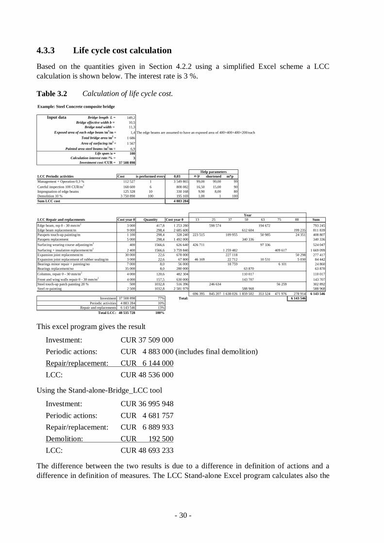
4.3.3 Life cycle cost calculation ............................................................................... 30
5. Discussion and proposal for future work ....................................................................... 32
6. Literature ...................................................................................................................... 33
- v -
Acronyms and notations Acronyms1
BaTMan The Swedish bridge and tunnel management system
BLCCA Bridge life-cycle cost analysis BMS Bridge management system CC Condition class CUR A general notation for currency, can be DKK, SEK, NOK, £, €, $,… ETSI Bridge Life Optimisation EXCEL LCC Life cycle costing LCP Life cycle plan MathCad A program system for engineering calculations MR&R Maintenance, Repair & Rehabilitation NVDB The Swedish national road database O&M Operation and maintenance TG1, TG2, TG3,… The ETSI project is performed within different sub-projects, and different task-groups are responsible. TG3 is responsible for the LCC subproject and TG4 for the LCA project. TrV Trafikverket, the Swedish Transport Administration WebHybris Software navigation tool that can access BaTMan database WLC Whole-life costing
Upper case roman letters1 (quantities)
,L rA Annuity factor ADT Average daily traffic/(vehicle/day) ADTt is the average daily traffic, measured in numbers of cars per day at time t, C0 Future cash flow expected to fall due every year during the service life-span L CACC Accident cost/CUR CEAC Equivalent annual cost/CUR CFA Average cost per fatal accident (CUR/accident) Ci Sum of all cash flows in year i /CUR CIA Average cost per serious injury accident (CUR/accident) CINS Inspection cost/CUR CINV Investment Cost/CUR CTDC Traffic delay cost/CUR CVOC Vehicle operating cost/CUR EAC Equivalent annual cost/CUR L Service life-span/a LCC Life-cycle cost/CUR LCI Life-cycle income/CUR
1 Acronyms should according to ISO be written in Romans style (upright). Quantities, always including a unit, should be written in italic (sloping style). The unit a (Latin annum) refers to ”year”. Year is not an allowed unit.
- vi -
Nt Number of days of road work at time t, PF Average number of killed persons in bridge related accidents (Persons/Accident) PI Average number of injured persons in bridge related accidents
(Persons/Accident) S is the length of affected roadway on which cars drive due to MR&R actions SDetour Detour length/m T Time studied/a. Usually the life-span (L) of the bridge WLC Whole life cost/CUR
Lower case roman letters1 (quantities) oD Average hourly operating cost for one passenger car/(CUR/h) oL Average hourly operating cost for one commercial truck/(CUR/h) pL Percentage of commercial traffic/% r Discount rate/% ri Inflation rate (%). rL Discount rate (%) for loans with long duration rTG Traffic growth rate/% t time/a vn Normal traffic speed, vr Traffic speed during bridge work activity/(km/h) wD Hourly time value for one passenger car/(CUR/h) wL Hourly time value for one truck/(CUR/h)
Indices All type cost items could be given an explanatory index. Some of the important indices are given above, but more are given in the text.
- 1 -
1. What is Bridge Life Cycle Costing 1.1 General The traffic infrastructure of a country is built to serve the society with roads, bridges, tunnels and other structures needed for an effective transportation sector. Taxes on vehicle fuel and likewise are used to pay for these services. The taxpayers want of course to get as much “value for money” as possible. The “value” is firstly a road system as effective as possible and with as few interruptions as possible for maintenance and repair. There are other values of importance concerning the environment, preserving energy and to use as little of not rene-wable material resources as possible. Very important values are also all kinds of traffic secu-rity issues. Other “values” could be esthetical or preserving old structures of historical inte-rest. The “money” in the “value for money” requirement could be investment cost, life cycle cost with or without user costs. There are many different views on how to calculate these kinds of costs. Some of these questions will shortly be discussed in this report.
This report on LCC is a part of the ETSI project. ETSI is interpreted as bridge life optimi-sation. This term is of course very general, but within the project it has been decided that only the situation when a new bridge is to be built, is studied. The tools developed are thus only suitable at this stage, where costs, environmental, aesthetical and cultural values are compared and the “best” bridge is to be sorted out and the early design stage.
1.2 Life Cycle Cost and BMS Life Cycle Costing, LCC, is a technique which enables comparative cost assessments to be made over a specified period of time, taking into account all relevant economic factors both in terms of initial capital costs and future operational costs. In particular, it is an economic as-sessment considering all projected relevant cost flows over a period of analysis expressed in monetary value. Where the term uses initial capital letters it can be defined as the present value of the total cost of an asset over the period of analysis.
Usually LCC is one important tool in a bridge management system (BMS). There are many other tools needed in a BMS, like LCA, but these will be described in other reports.
A bridge management system is usually divided into three levels:
• Country or county level
• Road or railway network level
• Project level, which usually is interpreted as a BMS for individual bridges.
There is however a close interaction between bridge LCC and BMS, because much of the information needed is the same. This means that, at least for individual bridges, the LCC can both be seen as a tool within the BMS or the LCC completed with some systems can be used as a steering system for the BMS.
One of the main requirements of a BMS is the control of reliability of the structures over time. The safety is controlled by condition constraints, i.e. by defining the lowest allowable condi-tion states for the bridge.
- 2 -
For both a BMS and for LCC the following information is needed:
• Definition of the bridge, its parts, elements, details and equipment with measures and quantities, also including relevant information about the relevant surrounding condi-tions. This information should be organised in a well-defined data inventory organised in a logical structural hierarchy. The data structure of the inventory must be consistent with the system needs.
• Planned management systems including maintaining an appropriate database of infor-mation
• Planned operation systems.
• Planned monitoring and rating systems.
• Planned alternatives for maintenance, repair and rehabilitation (MR&R) measures for the bridge parts and elements.
• Planned information on the use of the bridge like the amount and type of traffic flow.
• Planned demolition scheme.
Definition of these measures could be collected in a “Life cycle plan (LCP)”. If this plan is supplemented with economical information, like interest rates, and economical planning tools like the net present value method this can be called a LCC plan. It is an inherent condition that the LCC should be designed so that variation of the input values should be able to find an optimal solution for the LCP, because there are always economical constrains on the available resources for Maintenance, Repair and Rehabilitation (MR&R).
In a more general sense the LCC defining costs for the owner and the users, should be compared with a socio-economic income for the society. The bridge shall of course not being built unless it contributes to the social and economic development of the society.
1.3 LCC tools For simple cases it is rather easy to make simple LCC calculations i.e. using EXCEL or MathCad. In the ETSI project and at the department of Structural Engineering and Bridges at the Royal Institute of Technology (KTH), several LCC programs have been developed. A Stand-alone program based on EXCEL will be more in detail described in this report, but the principle of a web-based program will also shortly be discussed. A further development with more functionality will also shortly be discussed.
1.4 How to use the LCC tools The LCC tools are intended to be a part of the design process of bridges. The definitions, notations, see Chapter 3 are “ETSI-definitions” and are designed to be the “lowest common denominator” of the systems used in the Nordic countries. The idea is that the tools should be adapted to the methods used in each country.
Before starting the LCC calculation a “Life Cycle Plan” see the chapter on this issue, can be designed. This plan can contain the same type of information as the LCC program, but could
- 3 -
be more elaborated and the different items like actions could be explained and motivated. The plan can contain different options like variation of interest rate, use of different material qualities and so on. The LCC tool is then used for getting economical information on the options. Since the Life Cycle Plan and the LCC is a prognosis of the future, no exact values are expected, thus the LCC tools are mainly intended for comparison of different solutions.
- 4 -
2. Methodology for LCC calculation 2.1 The idea behind Life Cycle Cost analysis The classical task for the Bridge Engineer was to find a design giving the lowest investment cost for the bridge, taking the functional demands into consideration. Figure 2.1 shows this process schematically.
1) Technical design 2) Investment
Valuation
LowestInvestment cost
Figure 2.1 The classical task for the bridge engineer was to find the design giving the lowest investment cost for the bridge.
This process could result in a bridge design giving a low investment cost but high main-tenance costs. A LCC analysis aims in finding an optimal solution weighting investment and maintenance.
A comprehensive definition of Life Cycle Costing, LCC, is that it is a technique which enab-les comparative cost assessments to be made over a specified period of time, taking into account all relevant economic factors both in terms of initial capital costs and future opera-tional and maintenance costs. In particular, it is an economic assessment considering all pro-jected relevant cost flows over a period of analysis expressed in monetary value. Where the term uses initial capital letters, LCC, it can be defined as the present value of the total cost of an asset over the period of analysis. LCC calculation can be performed at any stage during the life-time of the structure, thus resulting in i.e. remaining LCC costs for an existing structure.
For making a complete LCC calculation for a bridge, at least the following parameters are needed:
1. Functional demands for the bridge. The most important of these demands are the safety, planned life-span and accepted traffic interruptions and user costs.
2. Physical description of the bridge. The structure is usually divided in parts, i.e. accor-ding to Table 2.1 and the different parts are given geometrical measures or weights.
3. Calculation methods for costs. This could be considered to be the LCC basic method including real interest rate calculations with known costs for operation, inspection, maintenance, repair, costs for accidents and demolition. Methods for this are discussed in Sections 2.3 to 2.7.
4. Time for interventions and incidents during the life-time of the bridge.
- 5 -
Point 4 is the most complicated point in an LCC calculation, since it must be based on known future events and behaviour of the bridge. And real knowledge of the future is of course by definition not existing. Tools for this point are though discussed in this chapter in Section 3.8. In Jutila & Sundquist (2007) Sections 4.6 and 4.6 a more thorough discussion on this question is presented. In this report it is assumed that the time between different maintenance and repair actions is decided by the user of the system, even if the WebLCC program presented in Chapter 4 has a module for modifying the time for actions depending on climate classes.
2.2 Basic calculation methods for LCC The different contributions in a complete LCC analysis of a structure could be divided into parts, mainly because different bodies in the society will be responsible for the costs occurring as a consequence of constructing or using the structures. There are many reports in this field i.e. Burley Rigden (1997), Hawk (1998), Siemens et al. (1985), Veshosky Bedleman (1992). The following presentation follows Troive (1998), Sundquist Troive (1998a and 1998b). In all these reports LCC is a general variable describing a cost, usually by using the net present value method calculated to the time of opening the bridge. The different parts of the calcula-tion can be described in Figure 2.2.
LCC
Agency costs
User costs
Society costs
Planning & Design
Construction
Maintenance
Disposal
Delay costs
Discomfort
Increased risks
Accidents
Environmental impact
Others
Upgrading
Operation
Repair
Inspections
Figure 2.2 Schematic presentation of the different items in a complete LCC analysis.
The owner - or in the case of an Agency like a Road or Railway Administration - has the re-sponsibility for investments, operation and MR&R costs. The user is the one who has the benefit of the road system and thus the bridges, but has also has to pay for lost working hours
- 6 -
due to traffic interruptions, risks and other problems. The society has to pay for accidents, en-vironmental impacts and if the road network does not function for the welfare of a country. The income for the society of the road and thus the bridge could be called LCI, Life Cycle Income.
In a general term the LCC should be smaller than the LCI. Typically a road system should not being built unless LCI is larger than 1,5·LCC, see Section 2.7.
It is very easy to use a toll bridge as an example for this scheme. The Income from tolls over a specified period of time should be larger than the depreciations, rents and MR&R costs for the bridge.
In the following only LCC will be discussed, and what can seem illogical, only the user costs will be included in the analysis. The society cost will only be included regarding accidents due to structural malfunction.
The environmental aspects will be treated in a special subproject (SP2) of the ETSI project. Cultural and aesthetic issues will be discussed in another subproject (SP3) of the ETSI project.
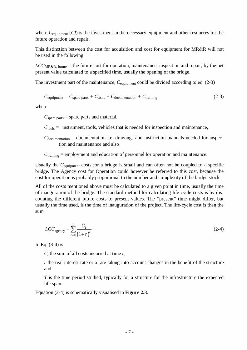
2.3 Agency costs LCCagency is the part of the total LCC cost that encumbers the owner of the project. This cost can in turn be divided into different parts according to Eq. (4-1)
LCCacquision (sometimes denoted LCCA) = is the cost for acquisition of the project including all relevant costs for programming and design of the project, by the net present value calculated to a specified time usually the opening of the bridge.
LCCMR&R (sometimes denoted LSC Life Support Cost) = is the cost for future operation, maintenance, repair and disposal of the bridge, by the net present value calculated to a specified time usually the opening of the bridge.
LCCconsequence (sometimes denoted LCCC = Life Cycle Cost Consequence) = is the future costs for possible negative consequences, by the net present value calculated to a specified time, usually the opening of the bridge. This kind of costs could possibly be a part of the user (LCCuser) or the society costs (LCCsociety), see below.
LCCsociety = is the future costs for possible negative consequences for the society, by the net present value calculated to a specified time, usually the opening of the bridge.
The LCCMR&R, the Life Support Cost (LSC), can in turn be divided into two parts according to Eq. (2-2)
LCCMR&R = Cequipment + LCCMR&R,future (2-2)
- 7 -
where Cequipment (CI) is the investment in the necessary equipment and other resources for the future operation and repair.
This distinction between the cost for acquisition and cost for equipment for MR&R will not be used in the following.
LCCMR&R, future is the future cost for operation, maintenance, inspection and repair, by the net present value calculated to a specified time, usually the opening of the bridge.
The investment part of the maintenance, Cequipment could be divided according to eq. (2-3)
Ctools = instrument, tools, vehicles that is needed for inspection and maintenance,
Cdocumentation = documentation i.e. drawings and instruction manuals needed for inspec-tion and maintenance and also
Ctraining = employment and education of personnel for operation and maintenance.
Usually the Cequipment costs for a bridge is small and can often not be coupled to a specific bridge. The Agency cost for Operation could however be referred to this cost, because the cost for operation is probably proportional to the number and complexity of the bridge stock.
All of the costs mentioned above must be calculated to a given point in time, usually the time of inauguration of the bridge. The standard method for calculating life cycle costs is by dis-counting the different future costs to present values. The “present” time might differ, but usually the time used, is the time of inauguration of the project. The life-cycle cost is then the sum
( )t
agency0 1
T
tt
CLCCr=
=+
∑ (2-4)
In Eq. (3-4) is
Ct the sum of all costs incurred at time t,
r the real interest rate or a rate taking into account changes in the benefit of the structure and
T is the time period studied, typically for a structure for the infrastructure the expected life span.
Equation (2-4) is schematically visualised in Figure 2.3.
- 8 -
Cos
ts
k k+ik+1 n n+1 m
Time/a1 765432 80
Investment
Repair
Major repair
Disposal
Yearly operation and maintenance costs
Figure 2.3 Schematically representation of agency costs for a bridge. The costs in this figure are not recalculated using the present value method.
When comparing investment projects of unequal life-spans, it would be improper to simply compare the net present values of the two projects unless neither project could be repeated to let all projects have the same analysis period. Equivalent Annual Cost (EAC) is often used as a decision support-tool in capital budgeting when comparing investment projects of unequal life-spans. In finance the EAC is the cost per year of owning and operating an asset over its entire life-span. The alternative associated with the lowest annuity cost is the most cost-effective choice. The EAC is calculated by multiplying the LCC calculated by the net present value by the annuity factor ,L rA :
net , net 1 (1 )L r LrEAC LCC A LCC
r −= × =− +
(2-5)
In an optimisation context the task, only taking the agency costs into consideration, is to design a bridge to find the lowest LCC. This phase of the LCC optimisation is visualised in Figure 2.4.
- 9 -
1) Technical design 2) Investment
Valuation
Lowest LCC cost
3) Operation, maintenance and disposal
Figure 2.4 The figure shows schematically the costs taken into consideration in a classic LCC analysis not including society and user costs.
Eq. (2-4) is usually used to calculate the owners cost for investment, operation, inspection, maintenance, repair and disposal.
The Ct costs at the time of inauguration are usually not too complicated to assume for the necessary above-mentioned steps in the management of a structure. There is a great uncer-tainty in choosing the r-value, but still more uncertain is the calculation of the time intervals between the different maintenance works and repairs.
To be able to assume the time intervals used for calculation, the degradation rate of the different parts of the structure must be known. Every structural engineer knows that this is a very complicated task. According to our knowledge the best information for assuming the time intervals is historical data from actual bridge inspections and repairs. Theoretical degra-dation models such as using carbonation rates, Fick´s second law or similar approaches seem, at this stage not to feasible. Combination of historical data with Markov-chain methodology seems however to be feasible if enough data is available.
2.4 User costs User costs (LCCuser) are typically costs for drivers, the cars and transported goods on or under the bridge due to delays due to roadwork. There are different kinds of user costs, like detours needed when the bridge is closed for repair etc., but these costs are very site-specific. Some other user costs are easier to calculate, because those are better related to the bridge itself.
Driver delay cost is the cost for the drivers who are delayed by the roadwork. Vehicle operating cost is capital cost for the vehicles, which are delayed by roadwork. Cost for goods is all kinds of costs for delaying the time for delivering the goods in time. Other user costs might be cost of damage to the vehicles and humans due to roadwork not included in the cost for the society. Travel delay costs can be computed using Eq. (2-6)
( )user,delay L L L Dr n0
1(1 )(1 )
T
t t tt
S SLCC ADT N p w p wv v r=
= − ⋅ + −
+ ∑ (2-6)
- 10 -
In Eq. (2-6)
S is the length of affected roadway on which cars drive,
vr is the traffic speed during bridge work activity,
vn is the normal traffic speed,
ADTt is the average daily traffic, measured in numbers of cars per day at time t,
Nt is the number of days of road work at time t,
pL is the amount of commercial traffic,
wL is the hourly time value for commercial traffic and
wD the hourly time value for drivers.
The costs should be calculated to present value and added up for all foreseen maintenance and repair work for the studied time interval T.
Vehicle operating costs and costs for transported goods can be calculated using Eq. (4-7)
( )user,operating L L G L Dr n0
1( ) (1 )(1 )
T
t t tt
L LLCC ADT N p o o p ov v r=
= − ⋅ + + −
+ ∑ (2-7)
In Eq. (4-7) the same parameters are used as in Eq. (4-6) except for
oL which are operating cost for the commercial traffic vehicles,
oG operating cost for transported goods and
oD operating cost for cars.
The costs should be calculated to present value and added up for all foreseen maintenance and repair work for the studied time interval T.
There is usually an accident cost for roadwork for the user not included in the cost for the society. Eq. (2-6) could be used also for this by just adjusting the cost parameter for this case.
- 11 -
1) Technical design
2) InvestmentValuation
Lowest LCC cost
3) Operation, maintenance and disposal
4) Society and user cost during main-
tenance and repair
Figure 2.5 The figure shows schematically the costs taken into consideration in a classic LCC analysis not including society and user costs.
2.5 Costs for the society Typical costs, not clearly visible for the Agency are costs occurring due to damage to the environment, the usage of non-renewable materials and society costs for health-care and deaths due to traffic accidents.
Most construction materials consume energy for production and transportation. One way to take this into account is by multiplying all costs for materials for construction and repair with some factor due to energy consumption for manufacturing and transportation. The use of non-renewable materials might be taken into consideration by involving costs for reproducing or reusing materials when the structure is decommissioned. These issues are discussed in the TG4 subproject on Life Cycle Assessment.
Costs for health-care due to accidents and deaths is probably only actual when two different types of structures are compared and when the risks for accidents differs between the two concepts, or costs for accidents due to roadwork. The accident costs for roadwork could be calculated using the formula
( )society, accident r n acc0
1(1 )
T
t t tt
LCC A A ADT N Cr=
= − ⋅ ⋅+
∑ (2-8)
In Eq. (2-8) An is the normal accident rate per vehicle-kilometres, Ar is the accident rate during roadwork and Cacc is the cost for each accident for the society, ADTt is the average daily traffic, measured in numbers of cars per day at time t and Nt is the number of days of road work at time t. The costs should be calculated to present value and added up for all foreseen maintenance and repair works for the studied time interval T.
As an example the Swedish Road Administration uses a cost of about 3 million $ for deaths and a third of that sum for serious accidents.
- 12 -
2.6 Failure costs There is a small risk for the total failure of a structure. To get the cost for failure one has to calculate all costs (KH,j) for the failure, accidents, rebuilding, user delay costs and so on and then multiply these costs with the probability for failure and with the appropriate present value factor according to the formula
( )failure H,1
11
nj j jjLCC K R
r==+
∑ (2-9)
In Eq. (2-9), Rj is the probability for a specified failure coupled to KH,j. For normal bridges the probability of failure is so small that the failure costs could be omitted in the analysis. The cost for serviceability limit failure is discussed in Radojičić (1999), but actually the methods presented in the present paper are a kind of statistically LCC-method given that the para-meters for remedial actions are considered random.
2.7 Comparing cost and benefit, whole life costing (WLC) Why a bridge – as a part of a road or railway – is built is of course that the project is con-sidered beneficial for the society. The income for the society of the road and thus the bridge could be called LCI, Life Cycle Income, and should of course be greater than the total LCC cost, see the schematically Figure 2.6. Calculation of the LCI is however not a part of this project.
1) Technical design 2) Investment
Valuation
Best societybenefit
3) Operation,maintenance and disposal
7) Society benefit and
lifetime
4) Society and user cost during main-
tenance and repair
Figure 2.6 A total cost benefit analysis shall of course also include both the total cost and the benefit for the society.
- 13 -
2.8 Interest rate The most important factor in Eq. (2-4) is, except of course the costs, the interest rate r. The real interest rate is usually calculated as the difference between the current discount rate for long loans and the inflation or more exact
L i
i1r rr
r−
=+
(2-10)
where
rL is the discount rate (%) for loans with long duration and
ri is the inflation rate (%).
The effect of the factor in the denominator is, taking the uncertainties into consideration, neg-ligible.
The inflation rate in the society might not be the same as the inflation rate for the construction sector. An investigation presented in Mattsson (2008) showed that the inflation in the con-struction sector in Sweden during the period was 1 % - 1,5 % higher than the general inflation rate, see also Figure 2.7. This fact shows a decrease in the productivity, but can also be ex-plained by stricter rules for safety measures that must be applied at the construction sites. This is especially true for maintenance and repair work on existing structures along the roads.
Figure 2.7 The “inflation rate” in the construction field in Sweden is higher than the general inflation rate in the society.
If there is a change in the benefit of the structure, i.e. an increase in the traffic using the bridge, this could approximately be taken into consideration by using the formula
L i TG
i1r r rr
r− −
=+
(2-11)
- 14 -
where rTG is the increase in traffic volume using the structure. If there is a risk for the opposite, a decrease in the usefulness of the structure, this factor should be given a negative sign. This could i.e. be accomplished by building the structure at the wrong place or on a road with decreasing traffic. Taking all factors into account the r-value should be called “calculation interest rate” or likewise. Typical values for r are in the order from 3 % to 8 %, see Jutila & Sundquist (2007).
2.9 Time between different MR&R actions To be able to calculate costs incurring at different times and then be able to discounting these costs to present values, one has to assume the time intervals for different measures that has to be taken during the life span of a structure. Typically a bridge needs to be inspected, main-tained and repaired many times during its life span.
Life span
One parameter of great importance is the planned service life span of the bridge. Standards often call for life spans from 40 to 120 years. Standards do not usually define the parameter “life-span” exactly. According to Mattson (2008), which is an interpretation of VBR Standard, the definition of life-span is the lower five percentile of the distribution of the life span. This interpretation means that the life span for 40, 100 and 120 year distribution is as shown in Figure 2.8.
In reality very few bridges survives such long lives. Due to the need for road rectifying, road widening, higher prescribed loads and changes in the society the actual service life of a bridge is shorter than the theoretical life span. In Sweden the average time for decommissioning bridges is in the order of 60 to 70 years.
0,0
0,1
0,2
0,3
0,4
0,5
0,6
0,7
0,8
0,9
1,0
0 20 40 60 80 100 120 140 160Year
Shar
e Su
rviv
ing
Min 40 Average 50
Min 80 Average 100
Min 120 Average 150
Figure 2.8 Standards calls for design life span of bridges, but at least in Sweden the design life span is defined as the lower 5 % fractile of a distribution that could be assumed to be normal distributed.
- 15 -
Time intervals for inspection and standard maintenance
All structures have to be inspected and maintained. The time intervals between these mea-sures depends on the type of bridge, the experience in the different countries, the economic resources available, the ADT value, the usage of de-icing salt and so on.
In Sweden all bridges are cleaned every year after the winter season and lightly surveyed. More profound inspections are performed every third or six year. These kinds of measures will of course vary between different countries and different owners. These types of measures will build up a part of the whole life costing for the owner of the bridge.
Inspection intervals in different countries are discussed in Jutila & Sundquist (2007). Defini-tions of the different types of inspections are different from country to country, so it not possible to directly compare the denomination and the intervals. In the Nordic countries only three main types of inspections are performed. Yearly very superficial inspection and general inspection every 5 to 6 year are performed. Special inspection must also be performed for more complicated cases. This must also be made allowances for in an LCC analysis.
Regular maintenance will of course always be needed. Typically railings, lampposts and other steel details need repainting regularly and this is could be considered being part of the yearly inspections.
Railings are often demolished by cars. The time intervals and the probability for these kinds of incidents are very dependent of the bridge type and the ADT-value.
Degradation models
All the discussed equations in Section 2.3 – Section 2.6 depend on information of lots of para-meters, many of which are very uncertain. One very important factor is the time intervals be-tween repair and maintenance work. These intervals for remedial actions are not fixed values as they are affected by the degradation and by considerations of which intervals that are most economical. It is here to mention that bridges usually do not just break down; it is their struc-tural elements that degrade.
There are different methods to forecast the degradation of different structural elements of bridges:
- One method is to use mechanistic or chemical models like Fick´s second law for diffusion of chlorides, carbonation rates, number of frost cycles and combinations to try to forecast degradation. Such a method is used by Vesikari (2003) and Söderqvist & Vesikari (2003). This approach is used in combination with the Markov Chain Method as a tool for analysis and this system is presented and discussed in section 3.8 in this report.
- An other method is to use and evaluate results from field observations, Racutanu (2000), Mattsson & Sundquist (2007).
- The up to day most applied method is to use experience from specialists, usually people deeply involved with inspection of bridges.
A special problem when using more sophisticated methods is to find suitable tools for going from degradation models to time predictions for MR&R actions.
- 16 -
3. Definitions and measures used in the ETSI LCC and LCA programs
3.1 Background To be able to have a consistent set of definitions for in- and output in the planned ETSI LCC and LCA there is a need to define and explain all parameters in the system. This document, mainly based on the Swedish system for such definitions as described in the BaTMan system, is a first preliminary suggestion for such definitions.
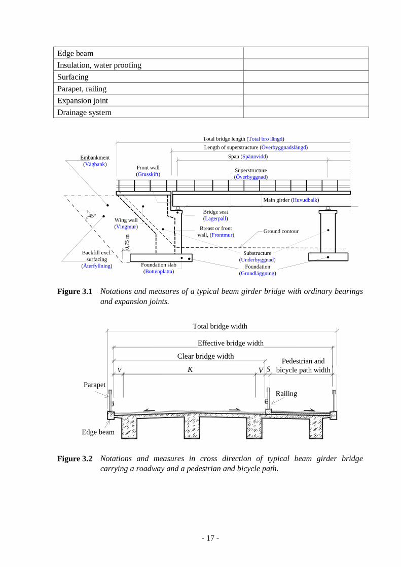
3.2 Definition of bridge parts and their measures Notion for bridge main structures and its elements are presented in Table 3.1.
Table 3.1 Notations for a typical girder bridge with ordinary bearings and expansion joints.
Description in English Explaining figure Foundation Foundation slab (base slab), plinth, pile cap Excavation, soil Excavation, rock Pile Erosion protection Slope and embankment Embankment, embankment end, backfill Figure 3.1 Soil reinforcement and slope protection Abutments and piers All concrete structures belonging to the substructure excl. foundation and including the foundation slabs
Figure 3.1
Main load-bearing structure Slab / deck Beam, girder Truss Arch, vault Cable system Pipe, culvert Secondary load-bearing structures Secondary load-bearing beam, cross beam Secondary load-bearing truss, wind bracing Equipment Bearing and hinge
- 17 -
Edge beam Insulation, water proofing Surfacing Parapet, railing Expansion joint Drainage system
Front wall (Grusskift)
Foundation slab(Bottenplatta)
Breast or front wall, (Frontmur)
Superstructure (Överbyggnad)
Main girder (Huvudbalk)
Substructure (Underbyggnad)
Wing wall (Vingmur)
Bridge seat (Lagerpall)
Span (Spännvidd)
Length of superstructure (Överbyggnadslängd)Total bridge length (Total bro längd)
Foundation (Grundläggning)
Backfill excl. surfacing
(Återfyllning)
0,75
m
45°
Ground contour
Embankment (Vägbank)
Figure 3.1 Notations and measures of a typical beam girder bridge with ordinary bearings and expansion joints.
S V GCV
Clear bridge width
Total bridge width
K
Effective bridge width
Pedestrian and bicycle path width
Total bridge width
Edge beam
ParapetRailing
Figure 3.2 Notations and measures in cross direction of typical beam girder bridge carrying a roadway and a pedestrian and bicycle path.
Figure 3.3 Notations in the longitudinal direction and in the cross direction for a typical box girder bridge with ordinary bearings and expansion joints.
Counterfort or buttress
Bearing
Expansion joint
Foundation slab
Integrated back or breast wall
Run on slabTransition slab
Bearing
Embankment endFront slope
Length of superstructure
Figure 3.4 Notations for abutment elements in an ordinary bridge and in an integral bridge with integrated back walls.
- 19 -
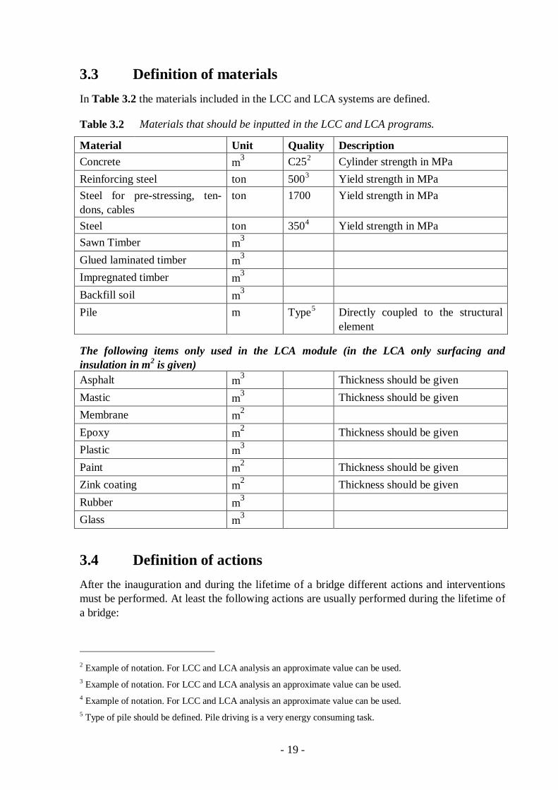
3.3 Definition of materials In Table 3.2 the materials included in the LCC and LCA systems are defined.
Table 3.2 Materials that should be inputted in the LCC and LCA programs.
Material Unit Quality Description Concrete m3 C252 Cylinder strength in MPa Reinforcing steel ton 5003 Yield strength in MPa Steel for pre-stressing, ten-dons, cables
ton 1700 Yield strength in MPa
Steel ton 3504 Yield strength in MPa Sawn Timber m3 Glued laminated timber m3 Impregnated timber m3 Backfill soil m3 Pile m Type5 Directly coupled to the structural
element
The following items only used in the LCA module (in the LCA only surfacing and insulation in m2 is given) Asphalt m3 Thickness should be given Mastic m3 Thickness should be given Membrane m2 Epoxy m2 Thickness should be given Plastic m3 Paint m2 Thickness should be given Zink coating m2 Thickness should be given Rubber m3 Glass m3
3.4 Definition of actions After the inauguration and during the lifetime of a bridge different actions and interventions must be performed. At least the following actions are usually performed during the lifetime of a bridge:
2 Example of notation. For LCC and LCA analysis an approximate value can be used. 3 Example of notation. For LCC and LCA analysis an approximate value can be used. 4 Example of notation. For LCC and LCA analysis an approximate value can be used. 5 Type of pile should be defined. Pile driving is a very energy consuming task.
- 20 -
• Management
• Inspection
• Operation
• Repair
• Upgrading
• Final demolition
Management is the owners own work for keeping the bridge inventory, the planning and other actions to manage the bridge stock.
Operation is the yearly work to superficially and regularly inspect, clean and to repair small damages of the bridges. The Swedish term is “Drift”. See also Table 3.4.
3.4.1 Management
Usually this work can be assigned as a percentage of the actual new construction value of the bridges in the bridge stock.
3.4.2 Inspection actions
Table 3.3 shows typical inspection actions and the intervals.
Table 3.3 Inspection types and intervals between inspections.
Inspection type Frequency Aims Remark
Regular Often (actually always!?)
Detect acute damages
Usually considered as part of the operation action
Superficial inspection
Twice a year (pro-bably only once a year)
Following-up of the yearly opera-tion maintenance (properties)
Usually considered as part of the operation main-tenance
Major inspection Every five to six years
Special inspection When needed
3.4.3 Operation
Maintenance actions could be divided into actions performed as part of the yearly operations and real repair actions needed when some of the structures or elements are severely damaged. Examples of such “Operation actions” are listed in Table 3.4, but could usually be calculated as a percentage of the cost to re-build the bridge stock. A typical value could be 0,2 %.
- 21 -
Table 3.4 Examples of “operation maintenance actions”. In the Swedish system this is called “Egenskaper” or “properties”.
Action Frequency Aim Remark
Regular inspection Often Detect acute damages
Cleaning of the bridge
Once a year Removal of de-icing salt
Rodding of dewatering system
Once a year
Cleaning of expansion joints
Once a year
Removal of plants and bushes,...
Once a year
3.4.4 Repair actions
Reference is made to BaTMan. (Just now I don’t have reference to these files). The Swedish word for these actions is “Åtgärder” or maybe in English “Measures”.
In Sweden the yearly average repair actions are in the order of 1 % to 1,3 % of the renewal value of the bridge stock.
3.4.5 Upgrading
Since the programs developed are to be used at an early stage of the bridge life, upgrading is not an issue at this stage and is not an action included in the LCC and LCA calculations.
3.4.6 Final demolition and reuse of material
Final demolition is a complicated issue, and very little research is performed regarding the reuse of material used for structures. Interesting points is the carbonisation of concrete during the demolition phase, especially if the concrete is crushed and used for road sub-grade. An approximate value is that the completely carbonated concrete “eats” half of the CO2-emis-sions from the cement production phase. The reused reinforcement steel requires less energy than the virgin steel. How much of the material from the demolition that is really reused is something nobody knows.
3.5 Environmental classes The degradation of structures due to different climate actions is a very complicated issue and has been a theme for an enormous amount of research during recent years. Degradation is
- 22 -
usually a combination of material properties in interaction with climate and issues coupled to the use and wear of the structure.
In the LCC aspect the material properties are defined by the used material as defined in Section 3.3. The environment and the use of the bridge must however be described in a way so that the degradation can be assessed by the user of the program. A very condensed subdivision of external deterioration factors is:
• Damage and wear due to use and
• Environmental damage.
Damage and wear due to use e.g.:
• Fatigue
• Progressive cracking
• Wear due to i.e. studded tires (mainly affecting the insulation and surfacing)
can approximately be set in proportion to the amount of traffic e.g. the average traffic volume ADT.
The environmental damage can be subdivided into
• Physical deterioration,
• Chemical deterioration and
• Reinforcement corrosion
The physical deterioration is typically
• Frost spalling (in cracks)
• Repeated frost-thaw cycles and
• salt crystallization.
The climate conditions affecting the physical deterioration are mainly the number of frost cycles and the salting. In the northern and in the most southern part of Scandinavia the number of cycles is not so large, so the severity of the climate in relation to physical deterio-ration is greatest in the central parts of the Nordic countries.
The chemical deterioration is to a large extent dependent of the material properties, but some factors as
• Carbonization,
• Chloride ingress,
• Reinforcement corrosion
Are highly dependent on
• Moisture,
• Road salting and/or rain with high content of salt and
• High temperature
- 23 -
In summary, the following parameters can very approximately define the climate and the external conditions in relation to the external conditions. A default value of all parameters is 1,0 i.e. factor = 1. A factor > 1,0 increases the time between repair actions, while a factor < 1 reduces the time between repair actions.
ADT:
ADT < 2000 factorADT = 1,1
2000 < ADT < 5000 factorADT = 1,0
ADT> 5000 factorADT = 0,9
Climate zone:
Northern Sweden (ekvi.) factorENV = 1,1
Central Sweden (ekvi.) factorENV = 1,0
Southern Sweden (ekvi.) factorENV = 0,9
Salting:
For roads with ADT > 10 000 and where lots of salt is used a factorL = 0,9 can be applied.
In total ADT ENV Lfactor factor factor factor= ⋅ ⋅ .
- 24 -
4. Program descriptions 4.1 LCC Stand-alone-Bridge-LCC program description The program Bridge-stand-alone-LCC consists of seven Excel spread sheets containing the following items:
Info: This sheet is always displayed at start-up and contains general information about the programme, as well as some important advice and instructions.
General conditions: In this sheet the general information necessary for the LCC analysis is input.
Investment cost; In this sheet the estimated investment cost based on the specified quantities and prices of materials is calculated.
Operation & Inspection cost: In this sheet costs and intervals for operation & maintenance activities and associated traffic disturbance is input.
Repair cost: In this sheet costs and the intervals for repairs and associated traffic disturbance is inserted and calculated. The calculation of the weighted intervals between actions is based on previously entered information about traffic, salt amount, concrete quality, etc.
Results: in this sheet a compilation of LCC costs presented both as tables and diagrams
Data:
Things to consider
This sheet contains important data the program uses during calculation. The user is not allowed to alter any of the cells in this sheet, why this sheet is not shown on start-up.
The user should consider the following points: 1. In order not to change the default settings and "default" values, always save the file
Bridge-Stand-Alone-LCC.xls under a new name before making changes / input for a new project.
2. Cells that have a small red triangle in the upper right corner contain the help text. The text becomes visible by hovering over the box. To view the help text clearly you might need to choose a larger text using "ZOOM" on the Excel window.
3. Never feed a space in a non-current cell. Enter instead a 0 (i.e. the number zero). 4. Users can choose the subdivision of bridge parts and elements as desired by changing
the text in each cell. 5. If no data is given for calculating the investment cost, the invest cost coming from
i.e. an offered cost from a contractor (entered in the General Conditions) will be used for the calculation of the total LCC.
6. At program start "default"-values are given in the new invented currency CUR for unit cost and intervals between actions. The default values at program start are approximate current (2010) units costs where CUR = SEK. The values must for each case be adapted to the project at hand, see point 1.
- 25 -
7. Repair and maintenance cost may also include cost for replacement of structural elements.
8. Repair intervals entered will be adjusted depending on the concrete quality, ADT, climate zone, salt amount, location of the bridge, and concrete cover. Weighting is not done if you enter yourself exact year for repair instead of intervals.
9. Repair interval should be chosen to receive a maximum of about 3 - 4 large steps during the bridge life by at least 10 years apart.
10. Quantities specified for calculating the cost of repair need not be the same as invest-ment quantities. E.g. you can choose to repair some of the concrete of the concrete slab superstructure instead of replacing the whole thing.
11. As road user cost the program includes only costs in the form of reduction in service benefits for as long as work is underway on the bridge and limited accessibility for the road users.
12. The LCC analysis should be done iteratively. Once the user has made the first run, the performance charts should be examined. The graphs show clearly the years, repairs and maintenance and also when these actions are carried out and their size. Users can thus be determined to manually move forward or backward in time to perform several actions at once. Remember, if necessary, also to change the number of days the road users are disturbed by the activity so these do not accidentally be added together and result in an overestimation of the road user costs. For example, if two activities are meant to be performed simultaneously only the activity with the longest duration gives any road user cost. This is of course depending on what activities are planned to be carried out and may not apply generally, therefore, the program do not make this correction automatically.
4.2 Principle design of the WebLCC program WebLCC is a program for doing Life Cycle Cost (LCC) calculations on the web. A LCC calculation summarizes all costs occurring during the intended life-span of a structure and recalculates these costs to a certain point in time, usually the time of inauguration of the structure using the net present value method. In the case of a bridge the LCC includes the construction, operation, repair work and the demolishing of the bridge at the end of the life-time. The calculation also includes indirect costs for the road users due to traffic interruption during repair work. WebLCC is sufficient general for making LCC analysis even for a small part of a large project. WebLCC also lets you in a simple and fast way to copy one project and use the data for i.e. comparing two different solutions for a bridge or a bridge part.
The WebLCC has many theoretical advantages, because all input is made dynamic, so there is no restrictions on how many inputs for actions that can be analysed.
There are however many practical problems with systems where all calculations are made on a central server. Bad things can happen when the user input wrong type of letters or numbers leading the server to break down.
If this program should be used in the future a professional Web programmer must be involved – resource not available at the division of Structural Engineering at KTH. The program is more in detail described in Salokangas L., (2009).
- 26 -
4.3 Case Study To describe the use of the Bridge-Stand-Alone-LCC program, a case study is performed. This case study is also shown when you first open the program. Remember to save your program under a new name, see Section 4.1 point 1.
The bridge is depicted in Figure 4.1 and Figure 4.2. The main properties of the bridge are compiled in the following section.
Figure 4.1 Horizontal and vertical view of the studied bridge.
Figure 4.2
Section of the studied bridge.
- 27 -
4.3.1 Input data:
Bridge Spans 45,5, 57,0 and 45,5, total bridge length incl. abutment structures 165,0 m. Length of the superstructure is 2 45,5 57 2 0,6 149,2m⋅ + + ⋅ =
Bridge effective width is 10,5 m, total bridge width incl. edge beams 11,3 m, assuming that the edge beams have an area of 20,4 0,4 0,16m⋅ = . Bridge area used for comparisons is
2149,2 11,3 1686m⋅ =
Bridge quantities are calculated using a methodology presented in a Power Point File “The material quantities and cost models by studies of Heikki Rautakorpi”. The PP-file is partly based on Rautakorpi H., “Material Quantity and Cost Estimation Models for the Design of Highway Bridges”, Acta Polytechnica Scandinavia – Civil Engineering and Building Con-struction Series, No. 90, 1988. Some of the notations used are according to the Finnish system.
Quantities:
For a steel concrete composite bridge deck the following applies:
The designation stands for an “average” span length calculated using the formula
2
0 1
1 ni
iL
L =∑ , where the lengths of the spans are denoted Li and n is the number of spans.
The number of piles are also given in Rautakorpi (1988), but are revised because of new higher allowed loads for piles.
- 28 -
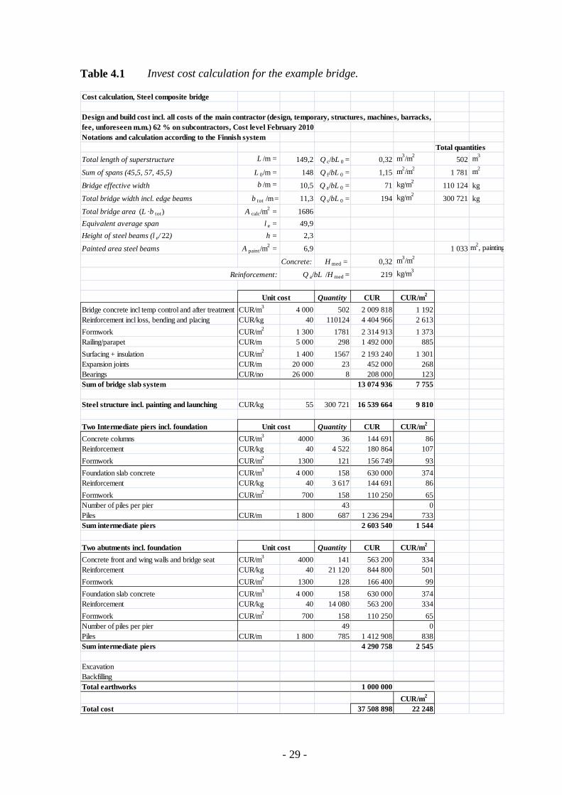
4.3.2 Calculation of quantities and investment cost
The formulas for calculation of quantities are presented in Section 4.2.1 are used and compiled in Table 4.1 below.
The investment cost is based on a Design and build contract. The unit costs includes all costs of the main contractor (design, temporary, structures, machines, barracks, fee, unforeseen etc.) 62 % on subcontractors. Cost level February 2010.
Quantities using the formulas above are compiled in an Excel file, together with the cost calculation. The total cost/m2 happens to be the current average cost for this kind of bridges in Sweden and if CUR = SEK, spring 2010 cost level.
- 29 -
Table 4.1 Invest cost calculation for the example bridge.
Cost calculation, Steel composite bridge
Design and build cost incl. all costs of the main contractor (design, temporary, structures, machines, barracks, fee, unforeseen m.m.) 62 % on subcontractors, Cost level February 2010Notations and calculation according to the Finnish system
Total quantitiesTotal length of superstructure L /m = 149,2 Q c/bL 0 = 0,32 m3/m2 502 m3
Sum of spans (45,5, 57, 45,5) L 0/m = 148 Q f/bL 0 = 1,15 m2/m2 1 781 m2
Bridge effective width b /m = 10,5 Q a/bL 0 = 71 kg/m2 110 124 kg
Total bridge width incl. edge beams b tot /m = 11,3 Q s/bL 0 = 194 kg/m2 300 721 kg
Total bridge area (L ·b tot) A calc/m2 = 1686
Equivalent average span l e = 49,9Height of steel beams (l e/ 22) h = 2,3
Painted area steel beams A paint/m2 = 6,9 1 033 m2, painting
Investment: CUR 37 509 000 Periodic actions: CUR 4 883 000 (includes final demolition)
LCC: CUR 48 536 000 Repair/replacement: CUR 6 144 000
Using the Stand-alone-Bridge_LCC tool
Investment: CUR 36 995 948 Periodic actions: CUR 4 681 757 Repair/replacement: CUR 6 889 933
LCC: CUR 48 693 233 Demolition: CUR 192 500
The difference between the two results is due to a difference in definition of actions and a difference in definition of measures. The LCC Stand-alone Excel program calculates also the
- 31 -
user costs, which however is not paid much attention in this example. The result is also presented in diagrams, see Figure 4.3 below.
Figure 4.3 Presentation of LCC results from the Stand-alone-Bridge-LCC program.
ETSI, Bridge Stand alone LCC Optimal new bridges - Life cycle analysis
5. Discussion and proposal for future work Making LCC calculations are a guess work on the future, and the only thing we really know about the future is that we don’t know anything. The big problem is guessing the degradation of the structures and thus the time between maintenance and repair actions. We must also guess rates of interest and inflation in the future. Locking in the rear-view mirror, we know that rates have changed dramatically over time. A good thing is though that the authorities in many cases have decided what rates to be used, but a discussion on this matter is Section 2.8.
Another factor of great importance is the structural degradation rates. An enormous amount of research has been devoted to physical and chemical degradation of concrete and steel struc-tures. Especially the ingress of chlorides and moisture and the following possible corrosion of the reinforcement has been studied for years, but the results is difficult to use as a prognosis for the needed maintenance and repair actions in the future. In the ETSI I report, Jutila A., & Sundquist H., (2007), a methodology based on Markov Chains in turn developed by Vesikari (2003) was presented. The input for this method is however complicated and with simple use it gave the wrong kind of curvature for the degradation curve.
As usual when guessing the future we have to use history and use regression analysis based on this data. A problem is however to find the historical data. A promising methodology for finding maintenance and repair historical data is to use the databases built up by the transport administrations. On-going research at the division of Structural Engineering and Bridges at KTH is by using historical data from the database BaTMan developed by the Swedish Transport Administration to predict future maintenance and repair actions and their associated cost. The costs in this database are calculated to current costs by the net present value method and should thus be rather reliable. For more information about these methods see Safi et al. (2012a) and Safi et al. (2012b).
Another maybe very good method is to collect data from LCC calculations made by experien-ced specialists on bridge element degradation and maintenance. This was an idea included in the WebLCC program, because all data was stored in a database coupled to this program. If in the future the WebLCC program is developed for better stability, this feature can be used for “research”.
After the research and development within the ETSI project, knowledge on LCC, LCA and “LCE” has been deepened, at least among the people involved in the three ETSI Stages. The next step is to bring the concepts and tools out in the practice. This will probably take a lot of effort, because the ideas on life cycle issues are not common practice among bridge engineers to-day. Probably the practical process of using LCC and LCA will influence the design of the tools, and new and better systems will be developed. Probably special tools will be developed for different purposes and for different stages in the design process for bridges, see e.g. Safi et al. (2012a).
- 33 -
6. Literature This literature list below refers mainly to bridge LCC studies. A more and complete general references to Bridge management systems, maintenance and management are given in Jutila & Sundquist (2007), ETSI Stage 1 report and to Salokangas (2009), ETSI Stage 2 report.
AASHTO (2001), Guidelines for Bridge Management Systems, American Association of State Highway and Transportation Official, AASHTO, Washington, D.C.
Abdel-Al-Rahim, I. & Johnston, D. (1993).
Estimating bridge related traffic accidents and costs. Transportation Research Board.
Abed-Al-Rahim, I., J. & Johnston, D.,W., (1995)
Bridge Replacement Cost Analysis Procedures. In Transportation Research Record No 1490, p.23-31, National Academy Press, Washington D.C.
Al-Subhi, K., M., Johnston D., W & Farid F., (1989).
Optimizing System Level Bridge Maintenance, Rehabilitation and Replacement Decisions. Report FHWA/NC/89-001.
Ansell A., Racutanu G., & Sundquist H., (2002)
A Markov approach in estimating the service life of bridge elements in Sweden, 9th International Conference on Durability of Building Materials and Components, Brisbane, Australia, 2002
ASTM E 917, (1994) Measuring Life-Cycle Costs of Buildings and Building Systems. American Society for Testing and Materials. 12 p.
Boyes D., S., (1995) Policy Traffic Management and Available Options, Bridge Modi-fication, 23-24 March 1994, Thomas Telford, London, pp 1-115.
Burley, E., Rigden, S., R., (1997)
The use of life cycle costing in assessing alternative bridge design, Proc. Instn Civ. Engrs, 121, p. 22-27, March, 1997.
Correialopes M., Jutila A., (1999)
Contracting Procedures, Design and Construction Costs for Bridges in European Countries, Helsinki University of Technology Publications in Bridge Engineering, TKK-SRT-25, Helsinki 1999.
COST 345 (2004), Procedures Required for Assessing Highway Structures – Joint report of Working Groups 2 and 3: methods used in European States to inspect and assess the condition of highway structures,
Davis Langdon Management Consulting,
Literature review of life cycle costing (LCC) and life cycle assessment (LCA). http://www.tmb.org.tr/arastirma_yayinlar/LCC_Literature_Review_Report.pdf.
de Brito, J. & Branco, F. (1998)
Computer-Aided Lifecycle Costs Prediction in Concrete Bridges, Engineering Modelling, Vol. 11, No. 3-4, pp. 97-106, University of Split/Zagreb, Croatia.
Ehlen, M. A., Bridge LCC 2.0 User Manual. Life-Cycle Costing Software for the Preliminary Design of Bridges. NIST GCR 03-853. http://www.bfrl.nist.gov/bridgelcc/UsersManual.pdf.
Ehlen, M. A., Marshall, H. E. (1996)
The Economics of New Technology Materials: A Case Study of FRP Bridge Decking, U.S. Department of Commerce, NISTIR 5864, Building and Fire Research Laboratory, National Institute of Standards and Technology, Gaithersburg, MD 20899.
Elbehairy, H. (2007). Bridge management system with integrated life cycle cost optimization. PhD Thesis, University of Waterloo, Waterloo.
Frangopol D., M., (1997)
Optimal Performance of Civil Infrastructure Systems, Proc. Int. Workshops on Optimal Performance of Civil Infrastructure Systems held in Conjunction with the ASCE Technical Committee on Optimal Structural Design Meeting at the Structural Congress XV, Portland USA, 1997.
Bridge Management Systems: Extended Review of Existing Systems and Outline framework for a European System. http://www.trl.co.uk/brime/D13.pdf.
Hallberg, D. & Racutanu, G. (2007).
Development of the Swedish bridge management system by introducing a LMS concept. Materials and Structures (2007) 40:627–639
Hawk, H. (2003). NCHRP Report 483: Bridge Life-Cycle Cost Analysis. TRB, National Research Board, Washington, D.C.
Hegazy, T. E. Elbeltagi, E & El-Behairy, H (2004).
Bridge Deck Management System with Integrated Life-Cycle Cost Optimization. Transportation Research Record: Journal of the Transportation Research Board, No. 1866, TRB, National Research Council, Washington, D.C., 2004, pp. 44–50.
Huang, R. Y. (2006). A performance-based bridge LCCA model using visual inspection inventory data. Construction Management and Economics 24, No. 10, 1069-1081.
Ingvarsson, H., & Westerberg, B. (1986).
Operation and maintenance of bridges and other bearing structures: State-of-the-art report and R&M needs. Swedish Road and Traffic Research. Swedish Transport Research Board.
ISO15686-5. (2008). Building and constructed assets-service-life planning. Part 5: Life-cycle costing. Stockholm: Swedish Standard Institute.
Jutila A., & Sundquist H., (2007).
ETSI PROJECT (STAGE I), Bridge Life Cycle Optimisation, Helsinki University of Technology Publications in Bridge Engineering, TKK-SRT-37, Espoo 2007.
Optimala nya broar, delstudie LCC-analyser, TRITA-BKN. Teknisk Rapport 2001:10, Brobyggnad 2001.
Leeming M., B., (1993)
The Application of Life Cycle Costing to Bridges, Bridge Manage-ment 2, Thomas Telford, London, pp 574-583, 1993.
Lindbladh, L. (1990). Bridge Management within the Swedish National Road Administration. 1st Bridge Management Conference, Guildford, Surrey, UK
Maes, M., Troive, S., (2006)
Risk perception and fear factors in life cycle costing, IABMAS -06
Markow, M. and Hyman, W. (2009).
NCHRP Synthesis 397: Bridge Management Systems for Transportation Agency Decision Making. TRB, Transportation Research Board, Washington, D.C.
Marshall, H., E., (1991)
Economic Methods and Risk Analyses Techniques for Evaluating Building Investments — A Survey, CIB Report Publication 136, February, 1991.
Mattsson H-Å., (2008)
Integrated Bridge Maintenance – Evaluation of a Pilot Project and Future Perspectives, PhD Thesis, TRITA-BKN. Bulletin 95, 2008, ISSN 1103-4270, ISRN KTH/BKN/B—95—SE.
Mattsson, H. & Sundquist, H. (2007).
The Real Service Life of Road Bridges. Proceeding of the Institution of Civil Engineering, Bridge Engineering, 160 (BE4), 173-179.
Mohsen, A., Shumin, T., Alfred Y. (1995)
Application of knowledge-based expert systems for rating highway bridges, Engineering Fracture Mechanics, Volume 50, Issues 5-6, March-April 1995, Pages 923-934.
NCHRP (2003) Bridge Life-Cycle Cost Analysis, National Cooperative Highway Research Program, Transport Research Board, NCHRP Report 483, Washington D. C., 2003. See also Hawk (2003)
NCHRP report 483: Bridge Life-Cycle Cost Analysis. Part I: P. 16. Part II: P. 9, 32-35 and 54-56.
Nickerson (1995) Life-cycle cost analysis for highway bridges, Proceedings of the 13th Structures Congress, Part 1 (of 2) Apr 3-5 1995 v1, Boston, MA, USA, pp 676-677, 1995.
OECD (1992) Bridge management, OECD, Road Transport Research, Paris 1992. ISBN 92-64-13617-7.
Ozbay, K., Jawad, D., and Hussain, S. (2004).
Life-Cycle Cost Analysis-State of the Practice versus State of the Art. In Transportation Research Record: Journal of the Transportation Research Board, No. 1864, TRB, Washington, D.C., pp. 62–70.
Patidar, V. Labi, K. Sinha K. &
NCHRP REPORT 590: Multi-Objective Optimization for Bridge Management Systems.TRB, Transportation Research Board,
- 36 -
Thompson P. (2007). Washington, D.C.
PIARC (1996) Type of Structures Selected for New Bridges, PIARC Committee on Road Bridges, World Road Association, 11.06.B, 1996.
Pritchard B., (1992) Bridge Design for Economy and Durability, Thomas Telford, London 1992.
R. Helmerich, R. Niederleithinger, E. Streicher, D. Wiggenhauser, V & Algernon D. (2008).
Bridge Inspection and Condition Assessment in Europe. Transportation Research Record: Journal of the Transportation Research Board, No. 2044, Transportation Research Board of the National Academies, Washington, D.C., 2008, pp. 31–38.
Racutanu G. (2000) The Real Service Life of Swedish Road Bridges – A case study. TRITA-BKN Bulletin 59, Dept. of Structural Engineering, Royal Institute of Technology, Stockholm, PhD thesis, 2000.
Racutanu, G., Sundquist, H., (1999)
Swedish Experiences of Integral Bridges, IABSE Symposium, Rio 1999.
Racutanu, G., Troive, S.,
Use of Empirical Database for the Evaluation of Service Life for Bridge Structural Members, Journal of Computer-Aided Civil and Infrastructure Engineering, April 1999.
Radojičic´ A., Bailey S., F., Brühwiler E. (2001)
Probabilistic Models of Cost for the Management of Existing Structures, ASCE, Structural Journal, 2001.
Rautakorpi, H., (1988)
Material Quantity and Cost Estimation for the Design of Highway Bridges, Acta Polytechnica Scandinavia No 90, Helsinki 1988.
Rigde,n S., R., Burley, E., Tajalli, S., M., A., (1995)
Life Cycle Costing and Design of Structures with Particular Reference to Bridges, Proc. Instn Civ. Engrs Mun. Engr, 109, pp 284-288, 1995.
Safi, M., Sundquist, H., Karoumi R., and Racutanu, G. (2012b)
Life-Cycle Costing Applications for bridges and Integration with Bridge Management Systems, Case-Study of the Swedish Bridge and Tunnel Management System (BaTMan), Transportation Research Record (TRR), Journal of Transportation Research Board (TRB), USA (2012)
Saito, M, Sinha, K.C. and Anderson, V.L (1991).
Statistical Models for the Estimation of Bridge Replacement Costs. In Transpn. Res.-A, Vol 25A, No. 6, pp. 339-350, Pergamon Press, UK.
Salokangas L., (2009) ETSI PROJECT (Stage 2), Bridge Life Cycle Optimisation, Report TKK-R-BE3, TKK Structural Engineering and Building Technology, Espoo.
- 37 -
Shepard (1993) “Using LCCA For Bridge Management System Applications”, FHWA Life-Cycle Cost Symposium, Washington, DC, December, 1993.
So, K. K. L., Cheung, M. M. S. & Zhang, E. X. Q. (2009).
Life-cycle cost management of concrete bridges. Proceeding of the Institution of Civil Engineering, Bridge Engineering, 162 (BE3), 103-117.
Söderqvist M-K. and Vesikari E., (2006)
Life Cycle Management Process, In: Sarja A. (Ed.), Predictive and Optimised Life Cycle Management. Buildings and Infrastructure. Taylor & Francis. London and New York 2006. Chapter 5. pp. 530 – 635.
Söderqvist M-K., and Vesikari E., (2003)
Generic Technical Handbook for a Predictive Life Cycle Management System of Concrete Structures (LMS), Lifecon GIRD-CT-2000-00378 Lifecon Deliverable D1.1, final report, Dec 2003. 170 p. http://lifecon.vtt.fi/
State of New Jersey. (2001).
Road user cost manual. Department Transportation, New Jersey.
Sundquist H., (1999) Optimala nya broar, Teknisk rapport 1999:8, KTH, Brobyggnad 1999.
Sundquist, H., Hans Åke Mattsson, H-Å., James G., (2004)
Procurement of bridge management based on functional requirements. In Second International Conference on Bridge Maintenance Safety and Management, IABMAS, Kyoto, Japan.
Sundquist, H., Karoumi, R, (2003)
Whole life costing and degradation models for bridges, ILCMI 2003, International workshop on integrated life-cycle management of infrastructures - bridges, Taipei, Taiwan, 2003.
Bridge Life-Cycle Costing in Integrated Environment of Design, Rating, and Management. Transportation Research Record: Journal of the Transportation Research Board, No. 1866, TRB, National Research Council, Washington, D.C., pp. 51–58.
Thompson, P. D., Campbell, J. A. Duray, A. R. Marshall, W. E. Robert, J. Aldayuz, and Hurst. K. F. (2003)
Integration of AASHTO’s BRIDGEWare Products. In Transportation Research Circular E-C049: 9th International Bridge Management Conference. TRB, National Research Council, Washington, D.C., April 2003, pp. 85–95.
Troive, S. (1998). Structural LCC design of concrete bridges. PhD Thesis, KTH-The Royal Institute of Technology, Department of Structural Engineering,
”Life-cycle Cost Analysis does not Work for Bridges”. Civil Engine-ering (Canada), July 1992.
Vesikari, E., (2003) Statistical Condition Management and Financial Optimisation in Life-time Management of Structures.” Part 1: “Markov Chain Based Life Cycle Cost (LCC) Analysis”. Part 2: “Reference Structure Models for Prediction of Degradation”, Lifecon GIRD-CT-2000-00378 Lifecon Deliverable D2.2, final report, Dec 2003. 113 p. http://lifecon.vtt.fi/
Vesikari, E., Söderqvist M-K. (2003)
LIFECON LMS Generic Technical Handbook for a Predictive Life Cycle Management System of Concrete Structures. Project for EC-CSG 5th RTD Programme (1998-2002), Contract No. G1RD-CT-2000-00378, LIFECON, Life Cycle Management of Concrete Infrastructures for improved sustainability, Deliverable D1.1, Final Report 2003, 170 p.