Bridge welding

8/9/2019 Bridge welding

http://slidepdf.com/reader/full/bridge-welding 1/162

Bridge Weigh-in-MotionDevelopment of a 2-D Multi-Vehicle Algorithm

Michael Quilligan

Department of Civil and Architectural EngineeringStructural Design and Bridge Division

Royal Institute of TechnologySE-100 44 Stockholm, Sweden

TRITA-BKN. Bulletin 69, 2003ISSN 1103-4270ISRN KTH/BKN/B--69--SE

Licentiate Thesis



© Michael Quilligan 2003



Acknowledgements

The research work presented in this thesis was undertaken at the Department ofCivil and Architectural Engineering, Structural Design and Bridge Division, at theRoyal Institute of Technology (KTH).

First of all, I would like to express my gratitude to Professor Håkan Sundquist forgiving me the opportunity to undertake this research at KTH. A very special thanksgoes to my supervisor Dr. Raid Karoumi whose endless help with all things Swedishand bridge related made my stay in Sweden all the richer.

This project formed part of a collaboration with University College Dublin (UCD). Iwould like to thank Professor Eugene O’Brien for introducing me to this subject area,and for his continued guidance, humour and advice. The prompt assistance andfriendship of Dr. Arturo González , especially regarding the FE model, is gratefullyacknowledged, as is the help of other members of the Bridge Research Group atUCD, notably Seán Brady .

The experimental work undertaken during the course of this study benefited greatlyfrom the persistence and kind help of Claes Kullberg of the KTH laboratory, Ales

Znidaric , Igor Lavric , Jan Kalin of ZAG, Robert Brozovic of CESTEL, and Dipl.-Ing.Eva Eichinger of the Technical University of Vienna. The support of Mats

Lundström, Mats Hagström and Benny Ersson of the Swedish National RoadsAdministration (Vägverket) is also sincerely acknowledged.

On a personal note, although one name appears under the title of this thesis, thework would not have completed but for the presence of many. Special mention goes

to my parents and sisters Laura and Gráinne , to Andrea and Esra for their endlesshumour in the office and while travelling, and to Liliana for putting up with methrough it all! I am thankful to all the people at the Department of Civil andArchitectural Engineering, especially the staff of the former Department of StructuralEngineering, for all their support and friendship.

Finally, this thesis is dedicated to Mr. Michael Punch . His inspirational thoughts andideals, dispensed during many a long journey to sites throughout Ireland, were notlost on the young student.

Michael Quilligan Stockholm, March 2003

i



ii



Abstract

Road transport and the related infrastructure are clearly an integral part of theeconomic, political and social development of the western world. Road pavements andbridges can be greatly damaged by excessively heavy vehicles. Great economies in thecost of road pavements can thus be achieved if truck and axle weights can bemaintained within legal limits. Consequently, there has been a considerable researcheffort at European level on technologies for weighing trucks (and axles) while theyare moving. The hope is that the accuracy of these so-called weigh-in-motion systemscan be enhanced to such a level that they can be used directly for enforcementpurposes.

Bridge Weigh-in-Motion (B-WIM) systems are based on the measurement of thedeformation of an existing bridge, and the use of these measurements to estimate theattributes of passing traffic. The purpose of this research is to enhance accuracy andusability of such B-WIM systems. B-WIM accuracy is heavily dependent on exactcalibration, i.e., the correct choice of influence line or influence surface. A new

method of influence line inference is presented. This matrix method has beendeveloped to provide a fully automatic and accurately calibrated influence line frommeasurements of the bridge response to a truck of known weight.

The B-WIM algorithm is extended to allow for the variation in the transverseposition of the truck on the bridge. This involves moving from an influence line to aninfluence surface. Various methods were employed to calculate the transverse positionof the crossing calibration vehicle. The calibration procedure to find the influencesurface, solely from experimentally measured data, is presented. The accuracy ofexisting B-WIM systems is strongly affected by the number of vehicles present on the

bridge during measurement. A B-WIM algorithm has been developed to cater formulti-vehicle events, thus removing unnecessary constraints regarding the operatingenvironment of future B-WIM systems.

The developed algorithms are verified using data from two test sites in Sweden andone in Vienna, Austria. A clear trend between erroneous results and the transverseposition of the crossing vehicle is noted. The study suggests that the accuracy of B-WIM systems can be significantly enhanced through the use of a 2-D algorithm,based on the use of an influence surface. Adoption of the 2-D algorithm is also shownto allow the accurate determination of vehicle weights during multi-vehicle events.

iii



A detailed Finite Element model of an instrumented bridge and calibration vehicle isconstructed and combined with a program that derives the interaction forces forbridge and vehicle models. These models are validated using measured data and anumber of simulations performed which confirm the suitability of the 2-D B-WIMalgorithm for such bridge types.

KEYWORDS: bridge, weigh-in-motion, WIM, influence line, influence surface,

calibration, accuracy, optimisation, multi-vehicle, simulation.

iv



Contents

Acknowledgements i

Abstract iii

Table of Contents v

1. Introduction 1

1.1 Weigh-in-Motion (WIM) Systems 1

1.2 Use of WIM Data 2

1.3 Aims and Scope

4

1.4 General Layout of Thesis 5

2. Literature Review 7

2.1 Static Weighing 7

2.1.1 Platform Scales 7

2.1.2 Portable Wheel Scales 8

2.1.3 Limitations of Static Weighing 8

2.2 Recent European WIM Research Programs 9

2.3 Accuracy Classification of WIM Systems 10

2.4 Pavement Based Weigh-in-Motion Systems 13

2.4.1 Introduction 13

2.4.2 Bending Plate and Load Cell Sensors 14

2.4.3 Strip Sensors 142.4.4 Multi Sensor-WIM (MS-WIM) 16

v



2.4.5 Testing of Pavement WIM Systems 17

2.5 Bridge Weigh-in-Motion Systems 21

2.5.1 Introduction 21

2.5.2 Moses’ Algorithm 222.5.3 AXWAY and CULWAY 22

2.5.4 DuWIM 24

2.5.5 SiWIM 26

2.5.6 Orthotropic B-WIM 28

2.5.7 Dynamic Algorithms 30

2.6 Conclusions 34

3. B-WIM Algorithms 35

3.1 Moses’ Algorithm 35

3.2 Influence Line Generation 37

3.2.1 ‘Matrix’ Type Method 40

3.2.2 General Form of Matrix Method 42

3.3 2-D Bridge Model 45

3.3.1 Influence Surface 46

3.3.2 Algorithm 52

3.4 Multi-Vehicle Presence 54

3.4.1 1-D Bridge Model 55

3.4.2 2-D Bridge Model 58

3.5 ‘Self-Calibration’ of B-WIM Systems 63

3.6 Conclusions 69

4. Experimental Tests 73

4.1 Introduction 73

4.2 Measurement of Transverse Position of Calibration Vehicle 75

4.2.1 Sand Method 75

4.2.2 Reflective Strips 76

4.2.3 Third Diagonal Tube 78

vi



4.3 Östermalms IP 79

4.3.1 Bridge Details 79

4.3.2 Axle Detection 81

4.3.3 Trial Details 834.3.4 Calibration 85

4.3.5 Results 89

4.4 Kramfors 96


4.4.2 Trial Details 98

4.4.3 Calibration 99

4.4.4 Results 103

4.5 Vienna 108


4.5.2 Trial Details 109

4.5.3 Calibration 110

4.5.4 Results 112

4.6 Summary and Conclusions 115

5. FE Simulations 119

4.1 Introduction 119

4.2 Bridge-Vehicle Interaction 119

4.3 Truck Model 120

4.4 Bridge Model 122

4.5 B-WIM 1254.6 Conclusions 127

6. Conclusions and Discussions 129

6.1 Introduction 129

6.2 Conclusions 129

6.2.1 Influence Line Calibration 129

6.2.2 Influence Surface Calibration 130

vii



6.2.3 Multi-Vehicle Events 131

6.2.4 Self-Calibration 132

6.2.5 Östermalms IP Trial 132

6.2.6 Kramfors Trial 1336.2.7 Vienna Trial 134

6.2.8 FE Simulations 135

6.3 Suggestions for Further Research 135

References 139

viii



Chapter 1

Introduction

Road transport and the related infrastructure are an integral part of a country’s

economic, political and social development. Recent decades have seen a rapid increase

in road and motorway traffic, and a major expansion in the number of heavy goods

vehicles on European roads.

Road pavements and bridges can be greatly damaged by excessively heavy vehicles.

The rate of deterioration of pavements in particular is known to be related to truck

static axle weight raised to the fourth power. Great economies in the cost of road

pavements can thus be achieved if truck and axle weights can be maintained within

legal limits. Accurate information regarding vehicle axle loads is also needed in order

to make prognoses on the development of traffic at all levels, and to be used as

parameters in the construction and maintenance of infrastructure projects.

Until recently the only method to control and monitor vehicle weights has been the

use of static weigh stations. This process can only weigh a very small portion of

vehicle population, and can lead to the collection of biased statistical data. To

overcome these limitations, a new paradigm in vehicle weighing has emerged, shaped

by a technology called weigh-in-motion .

1.1 Weigh-in-Motion (WIM) Systems

Weigh-in-Motion (WIM) is the process by which trucks and their axles are weighed

while the vehicle travels at full highway speed. There are primarily two categories of

WIM systems: pavement and bridge based.

Pavement systems consist of sensors embedded in or bonded to the pavement,perpendicular to the traffic direction (Figure 1.1(a)). These systems operate under

1



the principal that a particular measurable property of the WIM sensor varies

according to the load applied. Pavement systems record instantaneous dynamic axle

loads as a vehicle passes over the sensor. This occurs in a matter of milliseconds,

which gives an upper limit to the accuracy of these systems due to the short

recording time and the vehicle-pavement dynamics.

A Bridge Weigh-in-Motion (B-WIM) system is based on the measurement of the

deformation of a bridge, and the use of the measurements to estimate the attributes

of passing traffic. Such systems traditionally consist of two components (Figure

1.1(b)). The first is a device which monitors a varying property of the bridge

structure, usually longitudinal strain, using a strain sensor. The second component in

traditional B-WIM systems monitors the speed and axle spacing of the vehicles

crossing the bridge. Bridge systems can use the strain record while a vehicle crosses

over the bridge to determine axle weights. This passage is usually in the order ofseconds, and can therefore potentially reduce the error due to dynamic effects of a

vehicle travelling at speed.

(a) (b)

Figure 1.1 Weigh-in-Motion systems: (a) pavement based sensors record thedynamic axle loads as a vehicle passes over them; (b) B-WIM systemusing an existing bridge structure as a large scales (after Znidaric and

Baumgärtner 1998).

1.2 Use of WIM Data

The advent of WIM technology has allowed vehicle weights, both gross and

individual axles, to be estimated without the requirement of stopping the vehicle.

Unlike static weigh stations, WIM sites are located in the highway and can be almost

undetectable to passing vehicles. This enables the collection of unbiased traffic weight

data. Previous studies, including the Co-operation for Science and Technology 323

2



action (COST323 1999), investigated the applications of WIM data to both pavement

and bridge engineering. It was found that WIM data could be used for:

Enforcement Purposes

The cost of road maintenance, in the Netherlands for example, due to damage causedby overloaded trucks has been estimated at approximately 20% of their overall

pavement maintenance cost. It has been thought reasonable to assume that this cost

can be extrapolated to all European countries (Henny 1998). At the present time

WIM systems are being used for pre-selection of trucks in the UK, France, the

Netherlands, Portugal, Taiwan and Slovenia. In the UK and France there are Low

Speed WIM systems, while the Dutch High-Speed system integrates a video camera

with a WIM system for pre-selection of overweight trucks prior to enforcement using

static scales (Henny 1998). All of the systems have recorded promising results, but

have as yet failed to achieve the accuracy required for direct prosecution.

Improved Understanding of Pavement Performance

WIM can be used to evaluate the ‘aggressivity of the traffic’, i.e., determine the

number and magnitude of applied axle loads. It is this ‘aggressivity’ which causes

pavement damage. WIM results have shown that aggressiveness coefficients are

sometimes lower than would be expected, which has explained why some roads have

substantially less damage caused to them than was originally expected. Use of WIM

data can lead to improvements in pavement design and maintenance, hence reducingcosts (Caprez 1998).

Bridge Engineering

Eurocode 1, Part 3, ‘Traffic loading on bridges’ was the first bridge design code to

have used WIM data to calibrate traffic load models. WIM can also be used for the

design of long span bridges and in the assessment of existing bridges. During the

design phase of a typical bridge, notional traffic load models can be conservative due

to the uncertainty of traffic loads at the design stage. Good WIM-based models canremove some of this uncertainty and, as a result, unnecessary strengthening or

restriction of traffic can be avoided. WIM can also be used for dynamic impact

assessment to calculate the dynamic vehicle impact of trucks crossing a bridge. This

can be used for safety assessment or to calculate the load carrying capacity of

bridges. WIM can also be used for in-situ real time monitoring of the traffic loads on

bridges (O’Brien et al. 1998). For the design of long span bridges, Getachew (2001)

used a limited amount of WIM data in combination with the actual traffic

composition in order to calculate the appropriate queue weights.

3



Improving Road Safety

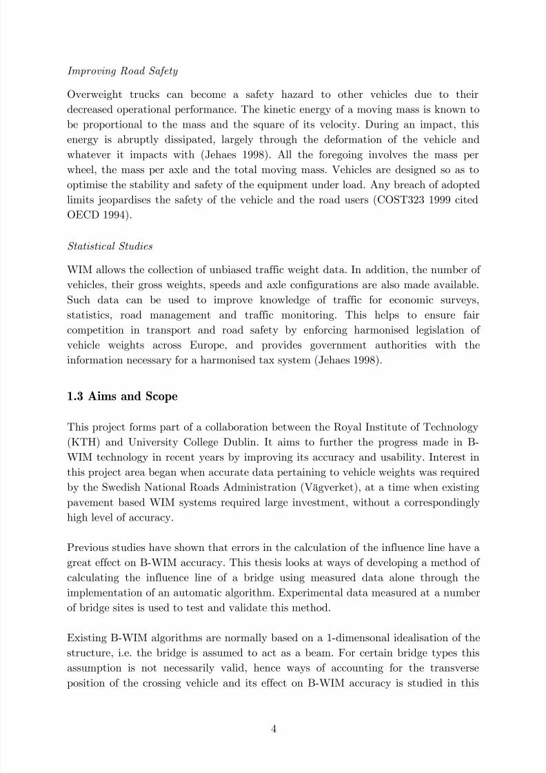
Overweight trucks can become a safety hazard to other vehicles due to their

decreased operational performance. The kinetic energy of a moving mass is known to

be proportional to the mass and the square of its velocity. During an impact, this

energy is abruptly dissipated, largely through the deformation of the vehicle andwhatever it impacts with (Jehaes 1998). All the foregoing involves the mass per

wheel, the mass per axle and the total moving mass. Vehicles are designed so as to

optimise the stability and safety of the equipment under load. Any breach of adopted

limits jeopardises the safety of the vehicle and the road users (COST323 1999 cited

OECD 1994).

Statistical Studies

WIM allows the collection of unbiased traffic weight data. In addition, the number ofvehicles, their gross weights, speeds and axle configurations are also made available.

Such data can be used to improve knowledge of traffic for economic surveys,

statistics, road management and traffic monitoring. This helps to ensure fair

competition in transport and road safety by enforcing harmonised legislation of

vehicle weights across Europe, and provides government authorities with the

information necessary for a harmonised tax system (Jehaes 1998).

1.3 Aims and Scope

This project forms part of a collaboration between the Royal Institute of Technology

(KTH) and University College Dublin. It aims to further the progress made in B-

WIM technology in recent years by improving its accuracy and usability. Interest in

this project area began when accurate data pertaining to vehicle weights was required

by the Swedish National Roads Administration (Vägverket), at a time when existing

pavement based WIM systems required large investment, without a correspondingly

high level of accuracy.

Previous studies have shown that errors in the calculation of the influence line have agreat effect on B-WIM accuracy. This thesis looks at ways of developing a method of

calculating the influence line of a bridge using measured data alone through the

implementation of an automatic algorithm. Experimental data measured at a number

of bridge sites is used to test and validate this method.

Existing B-WIM algorithms are normally based on a 1-dimensonal idealisation of the

structure, i.e. the bridge is assumed to act as a beam. For certain bridge types this

assumption is not necessarily valid, hence ways of accounting for the transverse

position of the crossing vehicle and its effect on B-WIM accuracy is studied in this

4



work. Experimental data from a number of bridge sites is predominantly used in this

investigation, however use is also made of a Finite Element (FE) model. This FE

model is based on one of the instrumented bridges and measured data is used in order

to validate the bridge and vehicle models.

A major disadvantage of current B-WIM systems is the inability to deal with events

whereby more that one vehicle is present simultaneously on the bridge. Dealing with

this issue forms a significant part of the work undertaken in this thesis as the ability

to deal with such events would greatly extend the applicability of B-WIM algorithms

to urban areas and longer span bridges where the probability of multi-vehicle events

is high.

All of the programming carried out in this thesis has been in the Matlab language

(The MathWorks 1999). Some expressions have been derived using the computeralgebra package Maple (Waterloo Maple 1996).

1.4 General Layout of Thesis

The work begins with a literature review on WIM systems. The study includes both

pavement and bridge based systems detailing the key aspects of their operation.

Particular attention is paid to the developments made in recent years in both the

COST323 and WAVE European research programs.

In Chapter 3, the basis of the B-WIM algorithm is introduced, beginning with Moses’

original algorithm. A method of influence line inference, termed the matrix method , is

presented which provides a fully automatic and accurately calibrated influence line

from measurements of the bridge response to a truck of known weight. This is

followed by the reasoning for moving from a 1-dimensional beam model to a 2-

dimensional plate model of the bridge. This involves moving from an influence line to

an influence surface. The calibration procedure to find the influence surface, solely

from experimentally measured data, is presented. A description of the issues involved

in catering for multi-vehicle events is given, followed by discussion of possiblemethods of ‘self calibration’ of B-WIM systems.

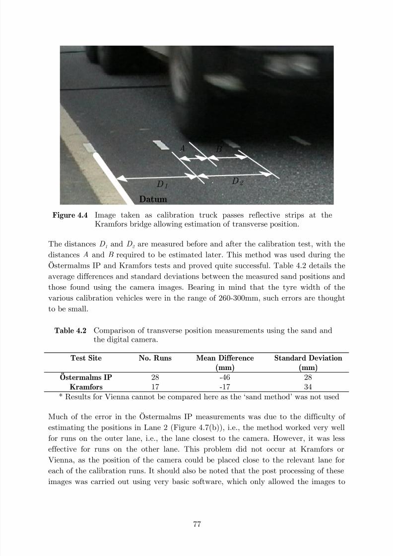
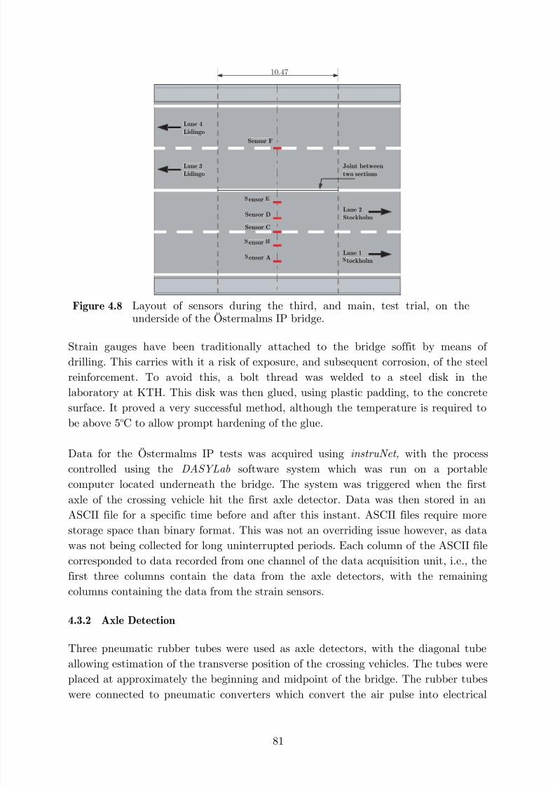
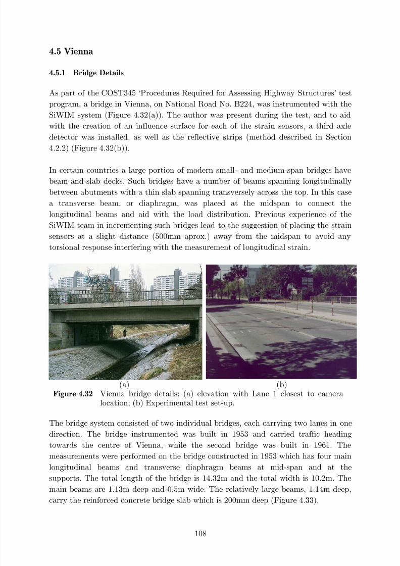
The next chapter details the experimental tests undertaken during the course of this

work. Short span integral type bridges have been found to be very suitable for the

purposes of B-WIM systems (Znidaric et al. 1998). As a result, two such bridges were

instrumented, one near Östermalms IP in Stockholm, while the other is close to

Kramfors in central Sweden. In conjunction with the COST345 Action - Procedures

for the Assessment of Highway Infrastructure, the author partook in a test on a beam

and slab bridge in Vienna, Austria. This bridge, located in an urban area, allowed thetesting of the developed algorithms on a different bridge type and in an area where

5



multi-vehicle events occur frequently. The experimental set-up, test plans and results

of these trials are detailed.

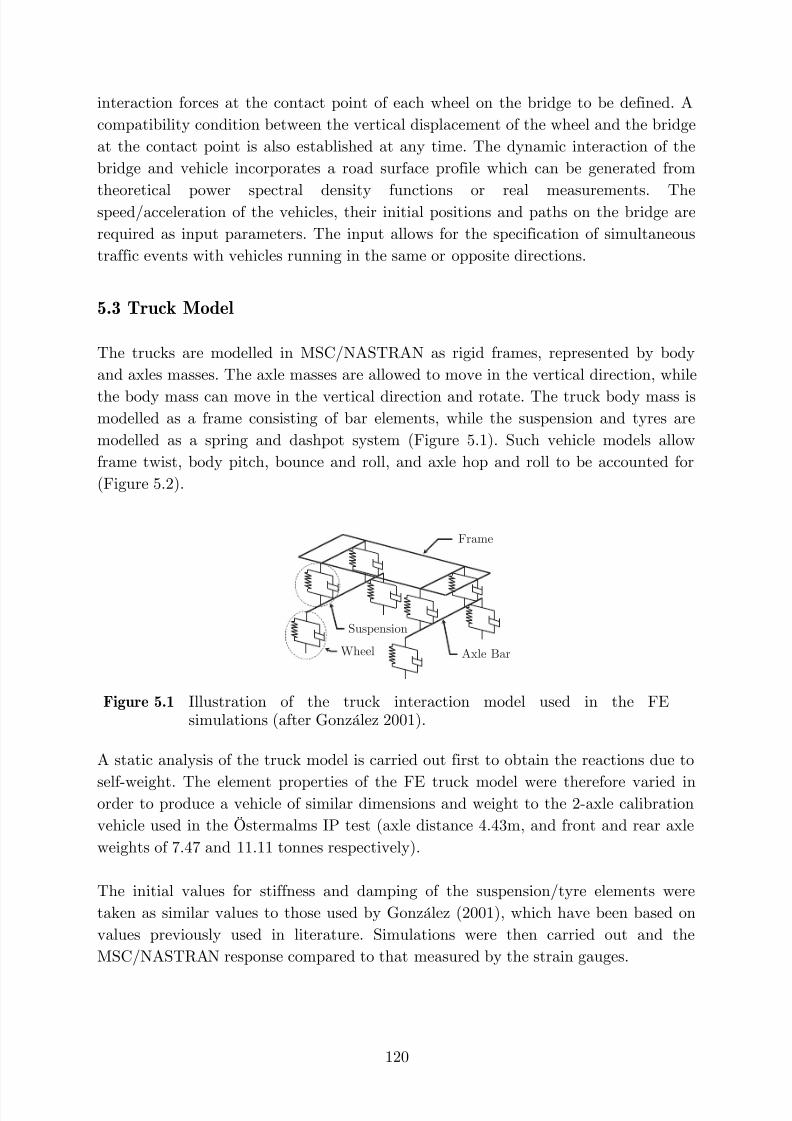
Chapter 5 concerns the finite element model developed using MSC/NASTRAN. This

model utilises a program, developed at UCD, that derives the interaction forces forbridge and vehicle finite element models. This enables the building of dynamic models

of both the bridge and truck. This model was validated using measured data from the

Östermalms IP bridge in Stockholm. A number of simulations were then performed,

and the suitability of the B-WIM algorithms monitored.

Finally Chapter 6 states the conclusions of this study, and directions for future

research are suggested.

6



Chapter 2

Literature Review

2.1 Static Weighing

The requirement to weigh civilian traffic vehicles is thought to date back to 1741,

when the UK Government of the day introduced the Turnpike Act, which decreed

that tolls were to be paid for the use of roads according to the weight of the vehicle.

Massive steelyards 1 were installed, but the vehicles had to be lifted before their

weight could be. The solution to this lay in the production of platform scales orweighbridges onto which the vehicles could be driven. From the late 1940’s

mechanical weighing began to combine with electronics, but it was not until the

invention of the load cell that complex and bulky lever systems and knife-edges were

replaced (Avery Berkel 1999). The two main types of static weighing systems in use

today consist of stationary platform and portable wheel scales. The accuracy of both

systems makes them eligible for enforcement purposes (Scheuter 1998).

2.1.1 Platform Scales

A truck scale consists of a scale frame that supports the weight of a truck without

major bending, a number of load cells, junction boxes, and a weight indicator. These

traditional platform scales are available in a wide range of sizes and weighing

capacities, in both pit-mounted and surface-mounted (Figure 2.1(a)) versions, with

steel or concrete platforms. These allow the Gross Vehicle Weight (GVW) to be

calculated to an accuracy of less than 0.5% (Scheuter 1998).

1 Invented by the Romans in 200BC, a steelyard consisted of a beam with a sliding poise tocounterbalance the load

7



(a) (b)Figure 2.1 Various means of statically weighing vehicles: (a) static weigh bridge

(after Avery Berkel 1999); (b) portable wheel load scales (afterMassload Technologies 2000).

2.1.2 Portable Wheel Scales

Portable wheel load scales (Figure 2.1(b)) have been developed to allow for

measuring wheel and axle loads, as well as GVW. Each wheel is measured

individually, although their precision is somewhat lower than platform scales.

Depending on how many scales are used, additional errors may be induced because of

weight transfer between axles due to longitudinal tilting of the vehicle, incorrect

sensor levelling, site unevenness, sensor tilting, mechanical friction in the suspension,

and residual friction forces induced by braking. The influence of these factors on the

results of axle group or GVW, is reduced by using the same number of scales as

number of wheels in the axle group or the whole vehicle. A set of 6 wheel load scalescan achieve a maximum error band of less than 1% for the GVW, but they are slow

and require a lot of labour. A set of 2 wheel load scales can achieve a maximum error

band of between 1% (good site and vehicles in good condition) and 3% (average site

and vehicles in poor condition) for the GVW (Scheuter 1998).

2.1.3 Limitations of Static Weighing

Static scales offer the advantage of allowing accurate calculation of the vehicle

weight. However, from a data collection and weight enforcement perspective, they aresubject to a number of drawbacks.

Benekohal et al. (1999) conducted a study at a static weigh station in Illinois were it

was found that 30% of all trucks could not be weighed because the weigh station was

temporarily closed to prevent a queue. In addition, the average truck was delayed by

approximately 5 minutes. Aside from the inconvenience imposed on truck drivers, a

greater problem exists with regard to avoidance of weight-enforcement stations by

overweight trucks. Cunagin et al. (1997) show that the number of overweight vehicles

decreases with increased enforcement activity, however vehicles attempt to bypassthese permanent truck weight-enforcement stations. It was found that violations at

8



the permanent weight-enforcement stations were minor, whereas those on the bypass

routes were much more severe. A total of 0.8% of the trucks were overweight at the

fixed scales, whereas 19% were in violation on the bypass routes during the study.

Recent B-WIM measuring campaigns in Sweden have shown that the level of

overloading cannot be estimated from static weighing, due to the avoidance of policeweighing locations by offending vehicles.

Taylor et al. (2000) and the Battelle Team (1995) reference studies in Virginia

(Cottrell 1992) and Wisconsin (Grundmanis 1989) where the problem of weigh

station evasion was also noted. In the case of Virginia, at two sites, 11% and 14% of

trucks were found to be overweight on routes used to bypass weigh stations, whereas

the figure grew to 20.3% in Wisconsin.

It is thought that truck operators will continue to operate overweight as long as theycan gain an economic advantage by either evading detection or paying a fine less that

the profit received from overloading (Cunagin et al. 1997). Weigh-in-motion offers a

solution to this problem by allowing vehicles to be weighed as they travel at full

highway speed, or as part of an integrated system where trucks can be pre-selected

via the WIM system prior to entering the weigh station (Figure 2.2). An added

advantage of B-WIM is that the main equipment is located under the bridge, making

it harder to detect, and hence avoid, that pavement based systems.

2.2 Recent European WIM Research Programs

Much of the recent research into WIM technologies has taken place as part of the

COST323 (1999) and WAVE (2001) programmes.

COST is an intergovernmental framework for European Co-operation in the field of

Scientific and Technical Research, allowing the co-ordination of nationally funded

research at a European level. The COST323 (1999) action was initiated by the

Forum of European Highway Research Laboratories (FEHRL), and formed part of

the COST-Transport program supported by DGVII (now DG TREN) of theEuropean Commission. It was the first European co-operative action on weigh-in-

motion of road vehicles. Eighteen countries participated, producing reports

concerning the needs and requirement for, and applications of WIM, a specification of

WIM systems, a glossary of terms, a European database, two conferences and some

large scale common tests of various systems (Jacob 1998).

WAVE (Weighing-in-motion of Axles and Vehicles for Europe) was a research and

development project of the fourth Framework Programme (Transport). The project

succeeded in improving the accuracy of WIM systems through the development ofimproved multi-sensor and Bridge WIM systems. Common data structures and a

9



quality assurance system were developed for WIM data as well as a new fibre-optic

WIM sensor. In addition, field trials were carried out under the harsh climatic

conditions of northern Sweden, and a heavily trafficked motorway in France (Jacob

and O’Brien 2002). Much reference is made to these programmes in the following

sections.

2.3 Accuracy Classification of WIM Systems

There are numerous applications for WIM systems, each requiring a particular

configuration and level of accuracy of measurement. To be able to evaluate and

compare the performance of these systems, it is necessary to define criteria for

evaluation or for acceptance. A European WIM specification has been prepared by

the COST323 management committee (Jacob and O’Brien 1998). This specification

gives an indication of what accuracy might be achievable from sites with particularcharacteristics, and what accuracy might be acceptable for various needs (Jacob 1997,

Jacob and O’Brien 1998).

This specification divides WIM systems into six classes of accuracy: A(5), B+(7),

B(10), C(15), D+(20), D(25) and E, with A(5) being the most accurate. The different

classes correspond to the different applications of WIM data. Class A systems could

be used for legal purposes, i.e., the enforcement of legal weight limits and commercial

weighing applications. Classes B and C can be used for infrastructure design and pre-

selection of vehicles for static weighing. Classes D and E would be used for statisticaldata of road traffic for economic purposes, etc. (Jacob and O’Brien 1998).

The WIM system accuracy classification is based on tests of measured results against

reference values, which are generally determined by statically weighing. The

measured results are compared with reference values, such reference values typically

being obtained by static weighing. Each class has a particular confidence interval

width, δ , for gross vehicle weight, group of axles weight, single axle weight and axle

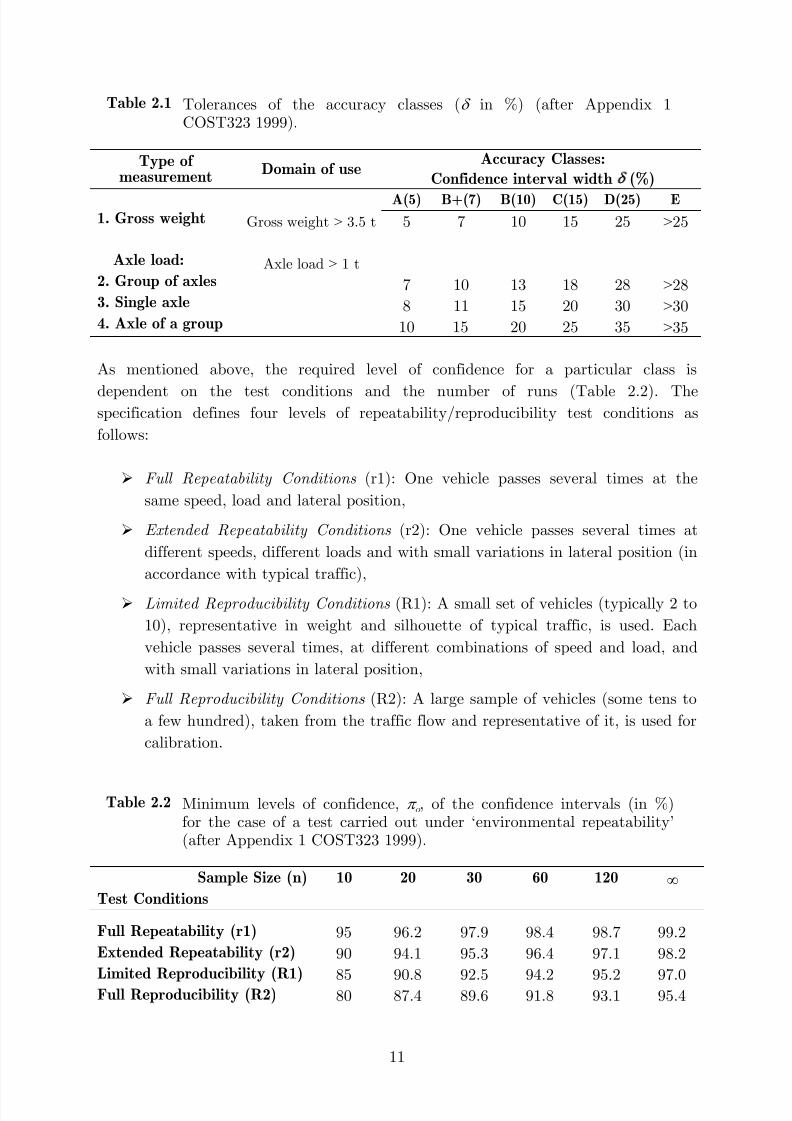
of a group weight (Table 2.1).

To comply with a given accuracy class, the calculated probability that results are

within the interval [W S (1-δ ), W S (1+δ )], where W S is the accepted reference value,

must exceed a specific minimum, π o . This minimum probability value, π

o , is a

function of the number of trucks, the duration of the test and the type of test carried

out (Table 2.2).

10



Table 2.1 Tolerances of the accuracy classes (δ in %) (after Appendix 1COST323 1999).

Type ofmeasurement Domain of use

Accuracy Classes:

Confidence interval width (%)

A(5) B+(7) B(10) C(15) D(25) E1. Gross weight Gross weight > 3.5 t 5 7 10 15 25 >25

Axle load: Axle load > 1 t2. Group of axles 7 10 13 18 28 >283. Single axle 8 11 15 20 30 >304. Axle of a group 10 15 20 25 35 >35

As mentioned above, the required level of confidence for a particular class is

dependent on the test conditions and the number of runs (Table 2.2). Thespecification defines four levels of repeatability/reproducibility test conditions as

follows:

Full Repeatability Conditions (r1): One vehicle passes several times at the

same speed, load and lateral position,

Extended Repeatability Conditions (r2): One vehicle passes several times at

different speeds, different loads and with small variations in lateral position (in

accordance with typical traffic),

Limited Reproducibility Conditions (R1): A small set of vehicles (typically 2 to

10), representative in weight and silhouette of typical traffic, is used. Each

vehicle passes several times, at different combinations of speed and load, and

with small variations in lateral position,

Full Reproducibility Conditions (R2): A large sample of vehicles (some tens to

a few hundred), taken from the traffic flow and representative of it, is used for

calibration.

Table 2.2 Minimum levels of confidence, π o , of the confidence intervals (in %)

for the case of a test carried out under ‘environmental repeatability’(after Appendix 1 COST323 1999).

Sample Size (n) 10 20 30 60 120 ∞ Test Conditions

Full Repeatability (r1) 95 96.2 97.9 98.4 98.7 99.2

Extended Repeatability (r2) 90 94.1 95.3 96.4 97.1 98.2

Limited Reproducibility (R1) 85 90.8 92.5 94.2 95.2 97.0Full Reproducibility (R2) 80 87.4 89.6 91.8 93.1 95.4

11



Tests may be carried out during various time periods, under environmental

repeatability or reproducibility conditions defined as (COST323 1999):

Environmental Repeatability (I): The test time period is limited to a few hours

such that the temperature, climatic and environmental conditions do not varysignificantly during the measurements,

Limited Environmental Reproducibility (II): The test time period extends over

at least a 24 hour period, or preferably over a few days within the same week

or month, such that the temperature, climatic and environmental conditions

vary during the measurements, but no seasonal effect has to be considered,

Full Environmental Reproducibility (III): The test time period extends over a

whole year or more, or at least over several days spread all over a year, such

that the temperature, climatic and environmental conditions vary during the

measurements and all the site seasonal conditions are encountered.

The statistical basis for the above classification was developed by Jacob (1997). In

this approach, it is assumed that an individual value is considered a relative error,

taken randomly from a Normally distributed sample of size n , with a sample mean m

and standard deviation s . A lower bound π , on the probability for that individual

value to be in the centred confidence interval [ ]; δ δ +− , is given at the confidence

level (1-α ) by:

)()( 21 u u Φ−Φ=π (2.1)

where 211 /)2/1(,/)( n t s m u v α δ −−−= , 21

2 /)2/1(,/)( n t s m u v α δ −+−−=

)2/1(,

, is the

cumulative distribution function of a student variable, and

Φ

α −v t is a student

variable with v = n - 1 degrees of freedom. The parameter α is taken to be equal to

0.5. Then the estimated level of confidence π , for each sample (and criterion) is

calculated using Equation 2.1. For the case of initial verification (same data used for

calibration and checking), δ is replaced by k .δ , where k is typically taken 0.8 (Jacoband O’Brien 1998). The accuracy level of the WIM system is then assessed using one

of two methods:

(i) For each sub-population (sample) corresponding to a criterion in Table 2.1,

and for the proposed (required) accuracy class defined by δ , the acceptance

test is:

oπ π ≥ , the system is accepted in that class,

oπ π < , the system cannot be accepted in the proposed accuracy class,

and the acceptance test is repeated with a lower accuracy class (a greaterδ ). π should be recalculated using Equation 2.1.

12



(ii) An alternative way is to calculate, using Equation 2.1, the (lowest) value

of δ which provides π = π o , and then to check that δ is less than the value

specified in Table 2.1 for the proposed accuracy class and criterion. This

approach allows a system to be classified in any accuracy class defined by an

arbitrary δ -value (the best one). Such a method has been implemented in anEXCEL macro by Jacob (1997) and has been used to classify the results of the

author’s B-WIM algorithms in Chapters 4 & 5.

2.4 Pavement Based Weigh-in-Motion Systems

2.4.1 Introduction

Pavement systems consist of sensors embedded in the pavement perpendicular to the

traffic direction. These systems operate under the principal that a particular

measurable property of the WIM sensor varies according to the load applied. Various

types of pavement sensor (and their associated systems) are available on the market

today, each having their own set of advantages and limitations. The first major

distinction between pavement WIM systems can be made between those that operate

at full highway speed, and those that require the vehicle to drive slowly over them,

namely High Speed and Low Speed systems.

A Low Speed WIM (LS-WIM) system is based on the same principle as static

weighing, and provides the high level of accuracy needed for enforcement purposes.

Vehicles are directed off the road and drive slowly (usually around 10km/h) over the

sensors (usually strain gauges or load cells) embedded in the surface. The full plate

LS-WIM system has a maximum permissible error band of between 1 and 5%

depending on installation conditions (Scheuter 1998). Portable systems are also

available, but require a long ramp before and after the scales to prevent oscillations

induced when the axles enter/leave the ramp. Such systems, with careful installation,

can meet the requirements for enforcement (expected to be A(5) according to

COST323 specifications) (Dolcemascolo et al. 1998).

13



Weigh-in-Motion

System

Roadside

Message Signs

Trucks Bypass

on the Main Line

Static Scale and

Inspection Station Figure 2.2 Pavement WIM system used to pre-select suspected overweight

vehicles (after ORNL and FHWA 2001).

High Speed WIM (HS-WIM) systems, which record axle weights as the vehicle

travels at full highway speed, are usually not as accurate as their LS-WIMcounterparts, with their accuracy much dependent on the quality of the sensor, site

location and approach. They can be used, combined with video software, to pre-select

vehicles for LS-WIM or static weighing (Figure 2.2) (Henny 1998). Such WIM sensors

can be divided into two categories according to their width: bending plate and strip

sensors.

2.4.2 Bending Plate and Load Cell Sensors

Bending plate WIM systems utilise metal plates with sensors attached to their

underside. As a vehicle passes over the metal plate, the system records the strain

(exerted by the rolling tyres) measured by the strain gauge and calculates the

dynamic load. Load cell WIM systems are available as two types, hydraulic and

strain gauge. When pressure is exerted on load cells, the hydraulic pressure is

measured and correlated to vehicle weight. Although configured differently, strain

gauge load cells operate similarly to bending plate strain gauge systems in that the

system records the strain (exerted by the rolling tyres) measured by the strain gauge

and calculates the dynamic load.

A major disadvantage of such systems is that for permanent installation in asphalt or

thin concrete roads, it is necessary to install a concrete foundation for support of the

frame. Such an installation, along with associated inductive loops or other axle

sensors, can take up to three days (Bushman and Pratt 1998). Load cell sensors may

also be used in portable applications, however, they can be quite inaccurate due to

truck motion induced by the protrusion of the sensor above the road surface.

2.4.3 Strip Sensors

Unlike bending plates, the width of a strip sensor only covers a portion of the wholetyre. The sensitivity of these sensors to factors such as truck dynamics, road

14



unevenness and temperature must therefore be taken into account during the

calibration of the WIM system (Scheuter 1998). Strip sensors are usually small in size

(20mm x 20mm x 1000mm) and are found embedded in grooves in the road. They

usually provide a more economical solution as they require less intrusion on the road

surface, but consequently their results are not as accurate. Strip sensors are availablein the form of piezoelectric, capacitive, quartz and fibre optic sensors, each of which

is now detailed.

Piezoelectric

The most common WIM sensor for data collection purposes is the piezoelectric

sensor. The basic construction of the typical sensor consists of a copper strand,

surrounded by a piezoelectric material, which is covered by a copper sheath. When

pressure is applied to the piezoelectric material an electrical charge is produced. The

sensor is actually embedded in the pavement and the load is transferred through the

pavement. The characteristics of the pavement will therefore affect the output signal.

By measuring and analysing the charge produced, the sensor can be used to measure

the weight of a passing tyre or axle group. There are a number of variations on the

shape, size and packaging of the sensors produced to obtain better results, easier

installation, and longer life (Bushman and Pratt 1998).

Piezo Quartz Crystal

The quartz sensor is based on a change of its electrical properties as a function of theapplied stresses. The quartz elements are mounted in a specially designed aluminium

extrusion. This section maximises the transfer of vertical load onto the sensing

elements whilst preventing lateral pressures from influencing the measurements

(Hoose and Kunz 1998). Piezo quartz have been found to be the most accurate of all

strip sensors during the Cold Environmental Test (Jehaes and Hallström 2002), as

well as in recent tests in the USA (McDonnell 2002) (see Section 2.4.5).

Capacitive Systems

A capacitive-based WIM system consists of two or more electrically charged metal

plates. As a wheel passes over the sensor, the upper plates deflect and the change in

capacitance is proportional to the applied load. Capacitive mat system layouts

typically consist of two inductive loops and one capacitive weight sensor per lane to

cover a maximum of four traffic lanes. In a portable set-up, the inductive stick-on

loops and the capacitive weight sensor are placed on top of the road pavement and

are meant to be used temporarily, sometimes up to 30 days. In a permanent set-up

the sensors are placed in stainless steel pans, flush-mounted with the pavement

(ORNL and FHWA 2001).

15



Fibre Optic

A fibre optic sensor ribbon is made of two metal strips welded around an optical

fibre. Under a vertical compressive force, the photoelastic properties of the glass fibre

result in separation in two propagating modes: a vertical faster mode and a slower

horizontal mode. The pressure transferred to the optical fibre creates a phase shift

between both polarisation modes, which is directly related to the load on the fibre.

Some of the reported advantages of fibre optic sensors include good operation from

stationary vehicles to speeds over 40m/s, low temperature dependence,

electromagnetic immunity, easy installation, no requirement for electric supply and

data processing in real time (Caussignac and Rougier 1999). The authors claim that

this technology can evaluate parameters such as tyre pressure, vehicle acceleration or

suspension condition.

2.4.4 Multi Sensor-WIM (MS-WIM)

A fundamental limitation in the performance of WIM systems is imposed by the

dynamic tyre forces due to vehicle-pavement interaction. As the width of a WIM

strip sensor is less than the impression of the tyre, the total wheel load will never be

exerted on the sensor at the same time. When a wheel passes the sensor, for a specific

period it will constantly measure a percentage of the total wheel load. To obtain the

total wheel load from the measured signal, the measured signal has to be integrated

with the passage time. The passage time is dependent on the speed at which the

truck drives over the sensor and the width of the sensor (van Loo 2001).

The total wheel load (F t ) is the product of the integrated measured signal (A), the

speed of the vehicle (V v ), the width of the sensor (Ls ) and a calibration factor (C ):

C ALV F s v t ××= )/( (2.2)

Due to irregularities in the road surface, a moving vehicle will, aside from its forward

motion, also move through the rocking, bouncing and hopping motion of the truck

and its axles. The form of the dynamic behaviour is largely determined by the mass,the distribution of the mass, the shock absorbers, the type of suspension of the

vehicle, and the road surface profile. When a vehicle is driving on the road, the axle

loads on the road surface will vary (dynamic axle load) around a static value (static

axle load).

The total axle load F (t) of a moving vehicle can be described, in simplified form, as a

combination of a constant static axle load (F o) and two periodical signals:

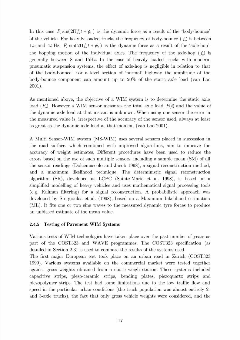
)2(sin)2(sin)( 21 φ φ +Π++Π+= t f F t f F F t F a a bbo (2.3)

16



In this case )2(sin 1φ +Π t f F bb

2(sin

is the dynamic force as a result of the ‘body-bounce’

of the vehicle. For heavily loaded trucks the frequency of body-bounce ( f b) is between

1.5 and 4.5Hz. )2φ +Π t f F a a is the dynamic force as a result of the ‘axle-hop’,

the hopping motion of the individual axles. The frequency of the axle-hop ( f a ) is

generally between 8 and 15Hz. In the case of heavily loaded trucks with modern,pneumatic suspension systems, the effect of axle-hop is negligible in relation to that

of the body-bounce. For a level section of ‘normal’ highway the amplitude of the

body-bounce component can amount up to 20% of the static axle load (van Loo

2001).

As mentioned above, the objective of a WIM system is to determine the static axle

load (F o). However a WIM sensor measures the total axle load F (t ) and the value of

the dynamic axle load at that instant is unknown. When using one sensor the error in

the measured value is, irrespective of the accuracy of the sensor used, always at leastas great as the dynamic axle load at that moment (van Loo 2001).

A Multi Sensor-WIM system (MS-WIM) uses several sensors placed in succession in

the road surface, which combined with improved algorithms, aim to improve the

accuracy of weight estimates. Different procedures have been used to reduce the

errors based on the use of such multiple sensors, including a sample mean (SM) of all

the sensor readings (Dolcemascolo and Jacob 1998), a signal reconstruction method,

and a maximum likelihood technique. The deterministic signal reconstruction

algorithm (SR), developed at LCPC (Sainte-Marie et al. 1998), is based on asimplified modelling of heavy vehicles and uses mathematical signal processing tools

(e.g. Kalman filtering) for a signal reconstruction. A probabilistic approach was

developed by Stergioulas et al. (1998), based on a Maximum Likelihood estimation

(ML). It fits one or two sine waves to the measured dynamic tyre forces to produce

an unbiased estimate of the mean value.

2.4.5 Testing of Pavement WIM Systems

Various tests of WIM technologies have taken place over the past number of years aspart of the COST323 and WAVE programmes. The COST323 specification (as

detailed in Section 2.3) is used to compare the results of the systems used.

The first major European test took place on an urban road in Zurich (COST323

1999). Various systems available on the commercial market were tested together

against gross weights obtained from a static weigh station. These systems included

capacitive strips, piezo-ceramic strips, bending plates, piezoquartz strips and

piezopolymer strips. The test had some limitations due to the low traffic flow and

speed in the particular urban conditions (the truck population was almost entirely 2-

and 3-axle trucks), the fact that only gross vehicle weights were considered, and the

17



rather poor pavement condition. Best results were obtained by a bending plate

system that achieved class C(15).

A further short trail took place near Trappes, France in June 1996 (Sainte-Marie et

al. 1998), where four portable and one multi-sensor WIM systems were used. Thefour portable systems (3 capacitive mats and 1 capacitive strip) recorded accuracy

classifications between E(30) to E(60), due to the dynamic impacts induced by the

thickness of the sensor above the road surface. The MS-WIM system performed much

better, with an accuracy classification of B(10) recorded.

A major test of WIM systems, termed ‘the European Test Program’ (ETP), was

conducted from 1997 to 1998. Its main objectives were (de Henau and Jacob 1998):

Evaluation of WIM systems in various environments and over long termperiods,

Comparison of the WIM system performances within the requirements of the

draft European specification and the users’ needs and requirements,

Acquisition of data for research and statistical studies.

The ETP consisted of two specific trials implemented at sites with different traffic

and climatic conditions: the Cold Environment Test (CET) and the Continental

Motorway Test (CMT). The CET was carried out on a main road in Northern

Sweden (near Luleå) in order to evaluate the performance and durability of WIM

systems in cold climates, whereas the CMT took place on a heavily trafficked

motorway in Eastern France. This site was chosen to monitor aggressive traffic

conditions, representative of main European routes.

The Cold Environmental Test (CET)

The pavement WIM systems tested during this test programme included a

piezoceramic nude cable, one prototype combination of two piezoquartz strip

sensors, a bending plate based on strain gauges and a ‘bending beam’ prototype. Inaddition, a prototype B-WIM system was located nearby and tested using some of

the same reference data. The test was managed by Vägverket, with the Belgium

Road Research Centre (BRRC) and the Institute of Road Construction and

Maintenance in Austria (ISTU) responsible for the analysis of the results (Jehaes and

Hallström 2002). The monitored road had two lanes and a class II profile according

to the European WIM Specification (COST323 1999).

Working problems were encountered with some of the systems, with all becoming

somewhat less accurate during the winter due to temperatures below -30˚C, orspring periods due to large temperature variations over 24 hours. All of them

18



recovered their initial accuracy during the following summer. Only the system based

on quartz crystal piezoelectric bars was able to achieve an accuracy class C(15)

throughout the test period. The results of this system in full environmental

reproducibility (III) and full reproducibility conditions (R2) are shown in Table 2.3.

Table 2.3

Accuracy classification of quartz crystal piezoelectric WIM systemunder full reproducibility conditions (R2) and full environmentalreproducibility conditions (III) (after Jehaes and Hallström 2002).

Criterion No.Mean(%)

St. dev.(%)

π

(%)Class

(%)min

(%) π

(%)Accepted

Class

Gross Weight 460 0.92 7.53 91.6 C(15) 15 13.9 94.0Group of Axles 838 1.41 7.33 92.0 C(15) 18 13.6 98.1 C(15)Axle of a Group 1721 1.41 10.02 92.4 B(10) 20 18.5 94.6

Single Axle 750 0.29 10.25 92.0 C(15) 20 18.7 93.9

To explain the implications of the above table, it is best to take the Gross Vehicle

weight category as an example. Here 460 runs were recorded for inclusion in the

analysis. The mean difference between the calculated WIM weights and the measured

static reference weights was 0.92%, with a standard deviation of 7.53%. To achieve

an accuracy classification of C(15), it is required that the probability that the results

are within 15% (δ - confidence interval) of the static values is above 91.6% (π o —

minimum level of confidence). The value for π o is determined by the number of runs,

460, and the test conditions, full reproducibility (R2) and full environmentalreproducibility conditions (III). In this case the recorded confidence interval, δ min, is

13.9%, with a confidence level, π , equal to 94%, i.e., 94% of the results are within +/-

13.9% of the static values, thus fulfilling the requirements of a C(15) classification.

The bending plate system obtained a final accuracy of D(25) (conditions R2, III) due

to a lack of temperature compensation over the winter period. The system used

temperature compensation in the summer achieving D+(20). The other two WIM

systems tested had accuracy classifications in class E (Jehaes and Hallström 2002).

Unlike the pavement WIM systems which were only calibrated in the first period, the

B-WIM systems was recalibrated before each test. Accordingly, direct comparison

cannot be made due to the differing test conditions. However, for the first period (1st

Summer) a comparison can be made in these conditions of environmental

repeatability (I) and full reproducibility. The bending plate gave the best results for

individual axle weights while piezo-quartz system was more accurate for axle groups.

However, a B-WIM system developed by University College Dublin, DuWIM (Section

2.5.4), was the most accurate for gross vehicle weights (significant considering the

problems encountered due to incorrect filtering and the failure of all but one strainamplifier) (O’Brien et al. 2002).

19



The Continental Motorway Test (CMT)

The CMT was the most significant large-scale trial ever organised in Europe, with

the objectives to evaluate commercially available WIM systems over a period of 12 to

18 months (Stanczyk and Jacob 2002). The reliability of sensors, electronic

equipment and software was also monitored. The test was carried out by CETE de

l’Est and the Laboratoire Central des Ponts et Chaussées (LCPC) in France. The site

is situated on the slow lane of the A31 motorway between Metz and Nancy with

international traffic of 40,000 vehicles/day, of which 20% are heavy vehicles. The

pavement is classified as class I according to the European specification (COST323

1999). The weighing sensors tested included four piezo-ceramic bars, a piezo-ceramic

‘nude’ cable and a capacitive mat.

The capacitive mat and one of the piezo-ceramic systems achieved class B(10).

Accuracy classes for the remaining systems ranged from C(15) to E(30) in conditions

of full reproducibility (R2) and environmental reproducibility (III). The results of the

piezo-ceramic system are shown in Table 2.4.

Table 2.4

Accuracy classification of piezo-ceramic WIM system (R2, III) (afterStanczyk and Jacob 2002).


St. dev.(%)

π

(%)Class

(%)min

(%) π

(%)Accepted

Class

Gross Weight 686 0.61 4.60 91.9 B(10) 10 8.46 96.2Group of Axles 588 2.63 5.97 91.8 B(10) 13 11.85 94.5 B(10)Axle of a Group 1328 2.67 8.49 92.2 B(10) 20 16.18 97.2

Single Axle 686 0.61 4.60 91.9 B(10) 10 8.46 96.2

The results for these systems remained stable throughout the year, due mainly to the

small temperature variations.

McDonnell (2002) reports high accuracy and repeatability using quartz-piezoelectric

sensors during extensive tests in the USA. After a complete reinstallation of the

sensors after a few months of operation, the author reported general satisfaction withthe working of the sensors which were placed, two per lane, in four lanes along

Connecticut Route 2. Results from a large number of pre-weighed vehicles

(approximately 1 000) were recorded over a three year period from 1998-2001. The

accuracy of the system varied from C(15) to B+(7), with best results attained in the

lane with the smoothest approach surface. However, warning was given regarding the

longevity of the sensors, due to the crack induced in the surrounding asphalt.

20



Current Testing Programs

Following the investigations of WAVE (2001), at least three European countries are

still active in the development of MS-WIM (Jacob and O’Brien 2002). In the

Netherlands, a 16-piezoquartz sensor array was installed in 2001 on a motorway by

the DWW for the Ministry of Transport (van Loo 2001) in order to check if this type

of sensor could provide a less noisy signal and better results than those obtained in

WAVE. In Germany, a project termed ‘Top-Trial’, supported by the EC, aims to test

a combination of several piezoquartz sensors and strain gauge scales in an MS-WIM

system for enforcement. In France, further investigations on MS-WIM are taking

place at LCPC, using computer simulations of vehicle-road dynamic interaction, to

assess the potential accuracy of the two developed algorithms under various

conditions, and to improve their implementation (Jacob and O’Brien 2002).

2.5 Bridge Weigh-in-Motion Systems

2.5.1 Introduction

A Bridge Weigh-in-Motion (B-WIM) system is based on the measurement of the

deformation of a bridge and the use of the measurements to estimate the attributes of

passing traffic loads. This technology generally consists of devices for measuring the

strain induced in the bridge by the vehicles, axle detectors for collecting information

on vehicle velocity and axle spacing, and data acquisition equipment. The

information provided by strain sensors and axle detectors is converted into axle

weights through the application of an algorithm. This algorithm obtains truck

weights by comparing theoretical models to a measured response.

As detailed previously, a major disadvantage of pavement WIM systems is that they

measure an instantaneous force for the time the tyre is supported on the WIM sensor.

This time depends on the sensor width and vehicle speed, and only a small portion of

the tyre oscillation is recorded. The deviations above or below the static value can be

well in excess of 30% on a pavement in good condition. If a WIM system is able to

measure the load for a full period of the lowest frequency, the problem of dynamic

oscillation would be overcome (WAVE 2001b).

The only existing WIM system capable of achieving this uninterrupted record is a B-

WIM system. B-WIM systems measure truck forces continuously as the truck travels

on the bridge. As the bridge length increases, the period of measurement increases

and lower frequency components of the force can be successfully detected. This is

simply not possible in pavement strip sensors due to the very short period of

measurement. The concept of B-WIM has therefore considerable potential for

accuracy as it makes possible the measurement of impact forces over more than one

21



eigenperiod of the vehicle. Further, B-WIM systems are durable as most of the

system parts are not on the road surface. B-WIM systems are also portable and can

readily be moved from one bridge site to another.

2.5.2 Moses’ Algorithm

In the 1970’s the Federal Highway Administration in the USA started studying the

use of Bridge-WIM systems to acquire WIM data. Moses (1979) developed a system

that used instrumented bridge girders to predict the axle and gross weights of trucks

in motion. The algorithm is based on the fact that a moving load along a bridge will

set up stresses in proportion to the product of the value of the influence line and the

axle load magnitude (the influence line being defined as the bending moment at the

point of measurement due to a unit axle load crossing the bridge). The bridge WIM

system described by Moses was the first of its kind and nowadays it is in use in theUSA and elsewhere.

Moses’ original system consisted of four parts: a button box, tape switches, strain

gauges and an instrumented van. The button box told the system of an oncoming

vehicle and initiated the recording of data. The tape switches were placed before the

bridge and determined the speed and axle distances of the crossing truck. Strain

gauges were placed on the soffit at midspan. The algorithm developed by Moses is

detailed in Chapter 3.

Results from initial test by Moses illustrated good repeatability of the results, with

standard errors reported to be under 10%. Further improvements were made to this

system (Moses and Ghosn 1983), and initial attempts were made to account for

multi-vehicle events. From analysis of the reported results it became clear to the

author, that while the errors for GVW were usually with 6% of the static values,

single and tandem axle results varied widely. This resulted in accuracy classifications

according to COST323 (1999), varying from D(20) to E(60)

2.5.3 AXWAY and CULWAY

In the 1980’s, Peters (1984) developed AXWAY in Australia. The system is based on

the assumption that the gross weight of a vehicle is proportional to the area under its

influence line. Unlike the employed by Moses, the gross vehicle weight is determined

by calculating the area under the recorded strain curve. The axle weights are then

varied in an iterative process to improve the fit between measured and expected

responses. The system is reported to give typical GVW accuracy within 3%, and axle

weights within 10% of static values for 90% of the cases, although details of the test

conditions were not reported.

22



The 17m single span bridge instrumented during the development of AXWAY had a

significant dynamic component corresponding to its first natural frequency. Peters

assumed this wave pattern to be sinusoidal of constant period and amplitude. By

integrating the measured response (due to both bridge and vehicle) over a

recommended four periods of this vibrational wave, Peters proposed that theremaining response would be due only to that of the vehicle (the integral of a

sinusoidal wave over any period being equal to zero). Such a technique however, also

results in corruption of the static response in cases of closely spaced axles and/or high

speeds. The system had the further disadvantage of requiring full time manning, as

real time processing of the data was not possible (using computers of that time) due

to the large number of iterations required.

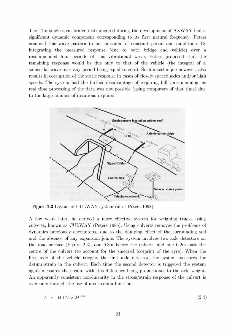
Figure 2.3 Layout of CULWAY system (after Peters 1998).

A few years later, he derived a more effective system for weighing trucks using

culverts, known as CULWAY (Peters 1986). Using culverts removes the problems of

dynamics previously encountered due to the damping effect of the surrounding soiland the absence of any expansion joints. The system involves two axle detectors on

the road surface (Figure 2.3), one 9.8m before the culvert, and one 0.2m past the

centre of the culvert (to account for the smeared footprint of the tyre). When the

first axle of the vehicle triggers the first axle detector, the system measures the

datum strain in the culvert. Each time the second detector is triggered the system

again measures the strain, with this difference being proportional to the axle weight.

An apparently consistent non-linearity in the stress/strain response of the culvert is

overcome through the use of a correction function:

855.00175.0 M A ×= (2.4)

23



where A is the corrected axle weight in tonnes, and M is the measured strain value

for that axle. A modification to Equation 2.4 is applicable if more that one axle is

present during measurement.

Peters (1998) reports a consistent seasonal variation in the accuracy of the CULWAYsystem at certain CULWAY sites. The exact reasons for this are not fully

understood. However the effects of seasonal moisture, temperature and stiffness

variation of the pavement materials are thought to be influential (this issue is dealt

with further in Section 3.5). To counteract this, an algorithm which applies a

monthly percentage correction to all measured values was developed. Grundy et al.

(2002a) studied the problem in further detail and using the knowledge that the

steering axle mass of articulated trucks within certain limits of axle configuration are

relatively constant, claimed to increase the accuracy of axle weight estimation by

removing seasonal and hourly drift. The applied correction factor for steering axlemass was determined on a weekly basis from the average steering axle mass of

selected trucks with six axles of single, dual and triple axle configuration. The daily

variation was then averaged over the whole period of data acquisition.

Spreadsheet based software, termed BRAWIM (Bridge Response Analysis from

Weigh In Motion data), has been developed to perform a statistical analysis of truck

data gathered using the CULWAY system at a WIM site in order to determine the

complete statistics of peak response, time at different levels of response, and

cumulative cycles of response for fatigue damage by Rainflow analysis for a specifiedinfluence line and span (Grundy et al. 2002b). This has illustrated the use of B-WIM

data for use in the monitoring of fatigue loading, and fatigue response spectra and

risk assessment of existing bridges.

2.5.4 DuWIM

Luleå Test

A series of B-WIM tests were carried out at a site adjacent to the COST323 Cold

Environment Test (CET) near Luleå, Sweden from June 1997 to June 1998 (McNulty1999, O’Brien et al. 2002). The data was processed independently by groups form the

Slovenian National Building and Civil Engineering Institute (ZAG), and a group

consisting of staff from Trinity College Dublin (TCD) and University College Dublin

(UCD), using different B-WIM algorithms. The algorithm developed by ZAG, known

as SiWIM, is described in Section 2.5.5, while that developed by TCD/UCD, referred

to as DuWIM, is discussed here.

The instrumented bridge is a two-span integral bridge with two equal spans of 14.6

m. Traffic is carried by one lane in each direction with no central median. As thedata collection of the DuWIM system was not automatic, the B-WIM system only

24



operated when TCD or UCD staff were present, namely, in June 1997 (1st Summer),

March 1998 (Winter) and June 1998 (2nd Summer). In all three cases, the system was

re-installed and re-calibrated; such re-calibration was not allowed for the pavement

systems taking part in the test proper (see Section 3.5). Data from strain transducers

was recorded and stored by TCD/UCD staff as the post-weighed (random) truckspassed over the bridge. The resulting raw data was subsequently post-processed. The

CET organisers did not release the static weights until all screening and processing of

results was completed, thus ensuring an independently monitored ‘blind’ test.

A unique feature of the DuWIM approach was a ‘point by point’ graphical method of

manually deriving the influence line from the bridge response to the calibration truck

(this method has been automated as described in Chapter 3). The results from the 1st

Summer test are shown in Table 2.5.

Table 2.5 Accuracy classification of the DuWIM system for 1st Summer test(after McNulty 1999).

Criterion No. Mean(%)

St. dev.(%)

πo (%)

Class(%)

min (%)

π

(%)Accepted

Class

Gross Weight 95 1.49 4.01 92.8 B(10) 10.0 8.6 96.6Group of Axles 162 2.09 5.93 93.5 B(10) 13.0 12.6 94.4 C(15)

Single Axle 156 -0.25 8.43 93.5 C(15) 20 17.0 97.2

The results deteriorated somewhat during the Winter test with an accuracy class of

C(15) recorded for each of the gross weight, group of axles, and single axle categories.

However a major problem with these first two tests resulted from the use of a 4 Hz

analogue filter in the data acquisition unit. This caused a loss of definition in the

bridge response and therefore, unfiltered data was used for the 2nd Summer test. For

this test, the results improved significantly, with an overall accuracy classification of

B(10) (Table 2.6).

Table 2.6

Accuracy classification of the DuWIM system for 2nd Summer test

(after McNulty 1999).


St. dev.(%)

πo (%)

Class(%)

min (%)

π

(%)Accepted

ClassGross Weight 122 -0.88 3.72 93.1 B(10) 10.0 7.7 98.4Group of Axles 239 -0.18 5.26 93.9 B(10) 13.0 10.6 98.0 B(10)

Single Axle 188 -1.31 7.27 93.7 B(10) 15 14.8 94.0

Multiple-Equation B-WIM (ME B-WIM)

The DuWIM system was also extended to use data from multiple sensors

longitudinally on the bridge (Kealy 1997). This method was developed to improve the

accuracy of B-WIM systems through the measurement of strain at more than one

25



location longitudinally along the bridge. This approach results in more equations

relating strains to axle weights at any given point in time. This goes some way to

solving the problem of varying axle forces, as complete history of such forces as the

truck crossed the bridge is provided. Kealy (1997) showed that instantaneous

calculation of axle and gross weights was theoretically possible provided the equationsrelating strains to weights are not dependent. This was shown to be possible for two-

axle trucks in single-span bridges and for three-axle trucks in two-span bridges. If it

is assumed that individual axles within tandems or tridems are of equal weight, then

three independent equations is enough to make instantaneous calculations possible for

most truck types.

The algorithm was tested on the two span continuous Belleville bridge on the A31

Motorway between Metz and Nancy in Eastern France. Gross weights were

calculated separately using data from each of the three longitudinal sensor locations.In addition, the mean of the three is presented. It was seen that, except for strain

gauge No. 3 (near central support), the ME B-WIM system was more accurate than

the conventional B-WIM system.

The poor results were, in part, attributed to the manner in which velocity and the

position of the vehicle on the bridge were monitored (a radar speed gun and a video

camera), and the poor magnitudes of recorded strain due to the excessive length of

the bridge (two 55m spans). It was felt by Kealy (1997) that the potential benefit of

getting an instantaneous applied dynamic force was not realised due to the highscatter of results. This would likely be improved through the use of a shorter bridge.

2.5.5 SiWIM

SiWIM is a B-WIM system that was developed at ZAG, Ljubljana, within the

framework of WAVE. It is now available as a commercial B-WIM system. After

using Moses’ algorithm for obtaining axle weights, SiWIM passes the results to an

optimisation algorithm, which has been shown to increase the accuracy of results

(Znidaric et al. 1998).

Luleå Test

The data collected during the Luleå test was also analysed using the SiWIM software

(WAVE 2001b). The accuracy classifications for the first two (1st Summer and

Winter) tests were similar to those achieved by the DuWIM system, i.e., C(15) for

both. For the 2nd Summer test, the results of the random traffic did not give

satisfactory results initially. The main reasons observed were several miss-matches of

the trucks weighed on B-WIM system and on the static scales and large temperature

variation during testing. Results originally produced a D(25) accuracy classification,although on adjustment, this was improved to B(10) (WAVE 2001b). It was noted

26



that during certain days of the experiment the temperature varied by up to 30o

(Figure 2.4). The strain sensors employed did not compensate for temperature, hence

required a linear correction factor to be applied afterwards, which resulted in

significant improvement of the results as noted above. The authors also suggest that

the deeply frozen soil unexpectedly influenced the bridge behaviour, with influencelines from the winter and summer test periods varying significantly.

Figure 2.4 Temperature dependency of Luleå B-WIM measurement (afterWAVE 2001b).

Extension to Slab Bridges

As part of WP1.2 of the WAVE program (WAVE 2001b) several different types of

short slab bridges were instrumented. One such instrumented bridge is located on the

A1 motorway near Ljubljana in Slovenia. The bridge is a 9o skewed integral bridge

with a 10m span. Although six strain transducers were installed, only one channel

was amplified properly, and consequently all results were based on strains from this

transducer alone. Several types of analysis were applied comprising of:

I. Theoretical influence line used (fixed supports assumed). Calibration factor for

all vehicles was obtained from the first five 5-axle semi-trailers - overall accuracyD(25).

II. Experimental influence line used in place of theoretical - overall accuracy

D+(20).

III. As above but 2 calibration factors were used: one for all semi-trailers based on

the first 5-axle semi-trailers and the other for all the rest based on the first five

2-axle rigid trucks (Method II calibration) - overall accuracy C(15).

IV. Results optimised trailers — overall accuracy C(15).

27



V. In addition, for all vehicles except for two-axle trucks, 4% of load from the first

axle was redistributed to all other axles (Method III COST323 1999) - overall

accuracy B(10).

The analysis showed that short slab bridges, previously only thought as conditionally

acceptable for B-WIM instrumentation (COST323 1999), offered few disadvantages

compared to longer beam-type bridges. The benefit of using an experimental influence

line, combined with an optimisation routine was shown to significantly improve

results. Interestingly, a need for higher calibration methods was shown to be

necessary for the case of articulated vehicles.

2.5.6 Orthotropic B-WIM

An important part of the WAVE research project involved the extension of B-WIM

to orthotropic bridges. In such bridges the steel plate is supported by longitudinalstiffeners, which span between transverse crossbeams. The light steel deck greatly

reduces the dead load of the bridge, significant in long span bridges, while allowing

composite action with the main girders, transverse beams and stiffeners. Therefore

the ratio of live to dead load is greater for orthotropic bridges than for other highway

bridges. This, combined with the fact that there are numerous weldings, means they

are highly sensitive to fatigue induced by traffic loads (Dempsey et al. 2000). The

extension to orthotropic decks involved two very important developments in B-WIM

technology, namely ‘Free of Axle Detector’ (FAD) and optimisation algorithms.

Free of Axle Detector (FAD) Systems

The Laboratoire Central des Ponts et Chaussées (LCPC), France, first considered the

idea of developing a B-WIM system without the use of road mounted axle detectors

in response to the requirements of the Normandy Bridge. In order maintain the

waterproofing of the deck, no axle detectors were allowed on the road surface as the

pavement was quite thin. A FAD system also offers the significant advantage of

removing the only component directly exposed to traffic, hence greatly improving the

durability of the overall system (WAVE 2001b).

The success of the FAD algorithm is greatly dependent on the general shape of the

measured strain signals under the moving vehicle. This shape has been found to be

dependent on the shape of the influence line, the bridge natural frequency, the ratio

between the span length and the (short) axle spacings, and the thickness of the

instrumented superstructure. As a result, short frame type bridges and longer span

bridges with thin slabs supported in the lateral direction by the cross beams or

stiffeners (i.e., orthotropic deck or similar bridges) have been recommended as

suitable for FAD instrumentation (Dempsey et al. 1999b). Longer span bridges areusually unsuitable due to the difficulties in distinguishing individual axles.

28



2-Dimensional Bridge Model

During experimental tests at the Autreville bridge in France (Figure 2.5), it was

found that the variation in transverse locations of the trucks within lanes had a

significant effect on the amplitude of the bridge response. This led to the

development of an optimisation algorithm based on a two-dimensional bridge model,

allowing for the different responses of the stiffeners depending on their position

relative to the transverse location of the truck (Dempsey et al. 1999a). This effect of

the transverse location on the accuracy was due to the sensitivity of the orthotropic

deck and the stiffening effect of the main I-beams of the bridge on the longitudinal

stiffeners closest to it. These influence lines were determined from a combination of

the experimental work and from the a detailed Finite Element (FE) model that was

constructed of the bridge. The requirement of such a detailed FE model was thought

to be a significant drawback to any potential B-WIM system, with the author

concentrating on producing influence surface solely from experimental data (Chapter

3).

Testing at the Autreville Bridge, France

The Autreville bridge in eastern France was instrumented in order to conduct the

initial tests, measurements and development of the above algorithms. The bridge was

chosen because of easy accessibility, and the fact that it is located on the same

motorway on which the Continental Motorway Test (CMT) was being conducted.

The bridge consists of three spans (74.5m, 92.5m and 64.75m), with the longitudinalstiffeners supported by transverse cross beams which span between two main I-beams

(Figure 2.5). The bridge was instrumented at three different longitudinal sections.

(a) (b)Figure 2.5 Autreville bridge in eastern France instrumented during the

development of the OB-WIM system: (a) elevation; (b) FEM meshfor one of the instrumented section (after WAVE 2001b).

Various trucks of different configurations and axle weights were stopped from the

traffic flow in August 1997 and July 1998. They were weighed statically axle by axle,

and the axle spacing, width of wheelbase and type of wheels (twin, single or wide

29



based) recorded. The transverse position of the trucks and the velocity of the truck

were also determined using an infra-red transmitter and receiver.

The FAD algorithm failed to identify only one of the forty-four trucks. The truck

which was not identified, had two different sets of unloaded closely spaced axles. Theaccuracy class obtained for each of the categories was found to be D+(20) for the 1-

dimensional bridge model, however this was improved to C(15) when the effects of

the transverse position of the vehicle were taken into account.

2.5.7 Dynamic Algorithms

Introduction

The traditional B-WIM algorithms have limitations when the dynamic behaviour of

the bridge-truck structural system does not follow a periodical oscillating patternaround the static response, as assumed by Moses (1979). These dynamic sources of

inaccuracy are related to the excitation of the dynamic wheel forces by the bridge

support or a bump in the approach (Lutzenberger and Baumgärtner 1999), or

measurements with a small number of natural periods of vibration (Peters 1984), or

bridges with low first natural frequencies, or the occurrence of a significant dynamic

amplification. If low-pass filtering of the signal is used to remove the effects of bridge

vibration, a significant part of the static response can be removed inadvertently, e.g.,

in the case of bridges with low natural frequencies, closely spaced axles and/or high

vehicle speeds (González and O’Brien 2002).

Previous research on dynamic systems has focused on the development of algorithms

in the time domain (Dempsey et al. 1998, O’Connor 1987). Such algorithms try to

correct the deviation from the static value that bridge and truck dynamics could

introduce in the measured strain. Most of these procedures yield a unique average

load as a result of using the whole strain record at one longitudinal sensor location.

However this assumption can induce significant errors due to the actually varying

applied load (WAVE 2001b).

More recent contributions from González (2001) have included an alternative

approach to calculating the influence line in the frequency domain, a dynamic

algorithm which takes account of bridge dynamics, and a dynamic multiple sensor

algorithm (MS B-WIM).

Dynamic Multiple-Sensor B-WIM (MS B-WIM) Algorithm

The Multiple-Equation (ME) B-WIM approach initiated by Kealy (1997) was

introduced in Section 2.5.4. It was noted that this static approach has limitations dueto the dependency of the equations which relate applied load to measured strain.

30



Hence the equations can only be solved for a limited number of axles. González and

O’Brien (2002) suggest that this limitation can generally be overcome by using a lot

of sensors (well in excess of the number of axles) and applying an optimisation

technique (González 2001).

Therefore if the number of sensors is greater than or equal to the number of axles, it

is possible to minimise the error function which compares the measured strain to the

theoretical static strain (using influence lines) or to the theoretical total strain. The

total theoretical strain at a certain location can be approximated as a function of the

applied axle weights and the total (static + dynamic) strain response due to a unit

moving. Figure 2.6(a) shows the midspan bending moment influence line and the

corresponding total strain response for a 20m bridge of natural frequency 4Hz. The

total strain corresponds to a moving load travelling at 20m/s. Unlike the static

component, the total strain for a given load depends on its speed, so there is adifferent curve taken as reference for each speed.

-1

01

2

3

4

5

6

7

8

9

0 2 4 6 8 10 12 14 16 18 20

Position of Moving Load (m)

S t r a i n

x

1 0 -

7

Influence Line Dynamic Response to a Moving Unit Load

0

20

40

60

80

120

100

140

160

4 9 14 19 24 29 34

First Axle Position (m)

A p

p l i e d F o r c e ( k N )

_

First AxleSecond Axle

(a) (b)

Figure 2.6 Details of dynamic algorithm: (a) midspan influence line anddynamic unit response (after WAVE 2001b); (b) calculated loadhistory using the MS B-WIM algorithm (after González and O’Brien2002).

The MS B-WIM algorithm was tested with data obtained from a 32m simply

supported beam and slab bridge in Slovenia. Strain transducers were placed at 6

longitudinal sections, two at each location (strains at each location were summed

producing six equations in total). From a record in free vibration, a damped

frequency of 3.5Hz and 5% damping were noted. A 2-axle truck with static loads of

34 and 127kN respectively for the front and rear axles, was driven over the bridge at

60km/h. The strain response for each longitudinal section was calibrated individually

using the spectral method. These curves were then used to calculate axle force on a

continuous basis. The results are shown in Figure 2.5(b).

31



As illustrated, a very good approximation of the static value can be obtained along

most of the bridge (except when an axle enters or leaves the bridge due to rounding

errors). González and O’Brien (2002) suggest that MS B-WIM can be a very accurate

method of weighing trucks for some particular sites, but further investigation on the

ideal number of sensors and their location, and experimental testing based on a widerrange of vehicles and speeds is still necessary.

Dynamic Algorithm based on Single Sensor Location

Applying the simultaneous dynamic equations at different sensor locations gives a

very similar instantaneous value along the bridge as was shown in Figure 2.6(b).

González and O’Brien (1998) used this hypothesis to develop an algorithm based on a

single sensor. The difference from Moses’ approach is the use of the dynamic response

due to a unit load instead of the influence line. This method was tested, with results

compared to the static and MS B-WIM algorithms, using a FE model.

Computer Simulation Testing of Dynamic Algorithms

Experimental test series can only measure a limited number of field parameters and

cover a small sample of bridges and vehicles. González (2001) constructed detailed

FEM bridge-truck interaction models, modifying the input to the general purpose

finite element analysis package MSC/NASTRAN, to allowed an in-depth study to be

conducted incorporating multiple bridge and vehicle types (this method was used by

the author and is detailed in Chapter 5).

Having tested the algorithm using four different bridge models, it was found that the

MS B-WIM can improve accuracy in individual axle weights over a single-sensor

algorithm. Overall MS B-WIM was the most accurate, except for bridges where the

response exhibits a low dynamic component or for sensor locations at the central

support in a two-span continuous bridge. In both these cases a static algorithm based

on one sensor location can be more accurate.

Though the MS B-WIM appears to be more accurate in most of the cases, such asystem would also require an expensive installation due to the extra number of

sensors required. The dynamic algorithm based on a single sensor location is not

thought to be a viable option, considering the extra numerical calculation required,

compared with the static algorithm, except for the longitudinal bending at midspan

of a two-span isotropic slab and voided slab deck.

The study by González and O’Brien (2002) also highlighted the fact that in some

cases, the traditional static algorithm could achieve better results by using types of

strain other than longitudinal bending at midspan, i.e., longitudinal bending of acentral support or transverse bending. Therefore, the choice of algorithm chosen is

32



very much dependent on the specific site, e.g., in bridges with high natural frequency

and low dynamics, a static B-WIM algorithm should be used, etc..

2.6 Conclusions

The recent period of intensive research activity in the weigh-in-motion area has

resulted in a deepening of knowledge and improvement in technology in the area. The

accuracy of both pavement and bridge based WIM systems has been greatly

increased, with the hope that MS-WIM systems can be used in the near future for

enforcement purposes.

However it is believed that with further enhancement that B-WIM has a natural

advantage due to the redundancy of recordings for a given vehicle event. This

redundancy should ultimately help B-WIM systems to improve their accuracy, whilethe implementation of the FAD systems will greatly increase the systems durability

and ease of installation.

33



34



Chapter 3

B-WIM Algorithms

3.1 Moses’ Algorithm

As detailed in Chapter 2, Bridge Weigh-in-Motion (B-WIM) originated in the USA in

the 1970’s, when a system was developed Federal Highway Administration (Moses

1978). The algorithm is based on the fact that a moving load along a bridge will set

up stresses in proportion to the product of the value of the influence line and the axle

load magnitude (the influence line being defined as the bending moment at the pointof measurement due to a unit axle load crossing the bridge). Moses used the fact that

each individual girder stress is related to moment from the relationship:

j

j j

W

M =σ (3.1)

where:

j = 1 … G (number of girders),

j σ = the stress in the th girder, j

j M = the bending moment in the th girder, j

j W = the section modulus.

The moment can be expressed in terms of strain as:

j j j j j EW W M ε σ == (3.2)

35



where:

E = the modulus of elasticity of the bridge material,

j ε = the strain in the th girder. j

Taking the sum of the individual girder moments, M , and assuming E and W as

constants:

j

∑∑∑ === j

G

j j j

G

j j EW EW M M ε ε (3.3)

Thus the sum of all girder strains is proportional to the gross bending moment. Total

bending moment and measured strain are therefore directly related by the product of

two constants ( . In theory, this constant can be calculated from bridge

dimensions and material properties, but in practice it is derived from measuring the

effect of the crossing of a truck of known weight over the bridge.

)EW

Weigh-in-motion analysis is therefore an inverse-type problem where the strain is

measured and the traffic load causing the strain is required to be calculated. The

theoretical bending moment caused by the number of axles on the bridge, at instant

k , is given by:

( )∑=

−=

N

i C i

T k

i k I AM

1

(3.4)

( ) v f LC i i /×= (3.5)

where:

N = the number of axles,

Ai = the weight of axle i ,

i C k I − = the influence line ordinate for axle i at scan k .C i = the number of scans corresponding to the axle distance Li ,

Li = the distance between axle i and the first axle in metres (L1, and hence

C 1, being equal to zero),

f = the scanning frequency in Hz,

v = the velocity in m/s.

In reality, bridge response is not static, but oscillates around a static equilibrium

position. Moses uses the fact that a lot of measurements are available during the

truck crossing to smooth out the dynamic components. The dynamic bridge responseis ‘filtered’ out by defining an error function, E , that minimises the sum of the

36



squares of the differences between the measured, M and theoretical, , strain

records:

M k

T k M

[ ]

2

1∑=

−=K

k

T

k

M

k M M E (3.6)

where

k is the scan number,

K is the total number of scans (readings),M k M is the measured bending moment at scan k .

Substituting Equation 3.4 into the above, and differentiating the error function, E ,

with respect to the axle weights, A, allows the unknown axle weights to be solved for

via a least squares fit between the measured and theoretical strains. This procedure is

dealt with in further detail in Section 3.4.

3.2 Influence Line Generation

Influence lines, which are used in practically all B-WIM systems, describe bridge

static behaviour under a moving unit load. For this application they are defined as

the bending moment at the point of measurement, i.e., sensor location, due to a unitaxle load moving along the bridge. The true influence line of many bridges lies

between the ideal simply supported and completely fixed support conditions (Figure

3.1).

Figure 3.1 Mid-span bending moment influence lines for simply and fixedsupported (integral) bridges (after Znidaric and Baumgärtner 1998).

Fixedsupports

A = 1A = 1

Simplysupported

37



Znidaric and Baumgärtner (1998) report on a study to monitor the effect of correct

choice of influence line on B-WIM accuracy. Two bridge lengths were chosen for this

study, a short 2m span and a longer 32m span. For the simulated signals, influence

lines within the two limit cases (the ideal simply supported and completely fixed

support conditions) were selected. The signals were later reprocessed using otherinfluence lines. The prediction of axle weights were shown to be very inaccurate if a

wrong influence line was chosen, especially for the longer 32m span bridge.

Results are summarised in Figure 3.2. While the error is below 10% for very short

bridges, and is similar for GVW and axle weights, errors of several hundred percent

were observed for the 32m long bridge. The greater the difference between the

integrals of measured and theoretical strains (areas under the corresponding influence

lines), the higher the error in the results. While in most cases the error in the GVW

is still within reasonable limits, the axle weights can be substantially redistributedleading to very large errors.

-30

-20

-10

0

10

20

30

fixed

supported

medium

(correct)

simply

supported

Influence Line (2-m span)

R e l a t i v e E r r o r ( % )

GVW Axle 1Axle 2 Axle 3Tandem

-300

-200

-100

0

100

200

300

fixed

supported

medium

(correct)

simply

supported

Influence Line (32-m span)

Tandem

GVW Axle 1Axle 2 Axle 3

R e l a t i v e E r r o r ( % )

Figure 3.2 Errors in weights for the two different bridge spans due to incorrectselection of the influence line (after Znidaric and Baumgärtner1998).

Correct calculation of this influence line is therefore of critical importance in the

search for accurate B-WIM results.

The influence line of a bridge can be easily derived through construction of arelatively simple frame model in a commercially available structural analysis package.

Support conditions can be assumed (rotational springs used if necessary) along with

the elastic modulus of the construction material, while the section modulus can be

varied in accordance with the bridge depth. Although this will allow reasonable

agreement between measured and theoretical responses, various factors such as

pavement flexibility, soil-structure interaction, ageing of constituent materials and

unknown support conditions render a theoretically calculated influence line unsuitable

for the purposes of B-WIM applications.

38



Previous approaches to the influence line calculation involved initially testing a

theoretical influence line, with modifications then applied to this curve to improve

accuracy. Znidaric et al. (1998) proposed revising the theoretical influence line by

adjusting the support conditions and smoothing the peaks interactively to take

account of the smeared footprint to achieve better conformity with the measuredresponse.

Ideally, it should be possible to make a ‘direct calculation’ of the influence line in stiff

bridges - high first natural frequency and low dynamic amplitudes (González and

O’Brien 2002). When there is only one axle on the bridge, as the mass of the axle is

known, it is possible to calculate the value of the influence line from the measured

strain record. When the second axle arrives on the bridge, its contribution to the

measured strain can be obtained from the known part of the influence line (already

calculated when the first axle passed that point). As the load effect caused by asecond axle on the bridge is known, the values of the influence line at the new

locations of the first axle can be obtained readily by discounting the effect of the

second axle. The same procedure can be applied to more axles arriving on the bridge.

20 4 6 8 10

0

-2

2

4

6

8

10

12

14

16x 10-3

Distance (m)

R e s p o n s e ( v o l t

s )

Correct IL`Direct Calculation'

Figure 3.3 Sample influence line derived using ‘direct calculation’ method —errors built up at beginning have a serious effect on the final shape.

In practice, this procedure is very sensitive to the small magnitude of the strains at

the start of the bridge and significant errors can be introduced in the first steps of

the calculation, making this approach prone to a build up of error (Figure 3.3).

McNulty (1999) developed a ‘point-by-point’ graphical method of manually deriving

the influence line from the bridge response to the calibration truck. A crude estimate

of the influence line is adjusted on the basis of a graphical comparison of theoreticaland measured strain in a spreadsheet program, usually EXCEL. Much of the

39



accuracy, B(10), of the DuWIM algorithm (see Section 2.5.4), has been attributed to

the success of this method. It can be used in all circumstances and requires little

knowledge of the bridge characteristics other than its length and position of supports.

It suffers from the disadvantage however, of requiring the manual adjustment of each

point.

González and O’Brien (2002) suggest calculating the influence line in the frequency

domain. The spectrum of the influence line is obtained by calculating the unit

contribution of all readings to a given frequency. The limitations of a direct

calculation in the time domain, as listed above, or the inconvenience of an

experimental adjustment, point by point, are overcome.

As illustrated by the above authors, for a robust and accurate B-WIM system, it is

desirable to have a method of influence line calibration that uses the measured strainsfrom the specific bridge, and requires minimal time and input from the operator. To

satisfy these conditions, a ‘matrix method ’ has been developed by the author to

provide a fully automatic and optimal Influence Line Generation algorithm, without

the need to enter the frequency domain.

3.2.1 ‘Matrix’ Type Method

Although Equation 3.6 was used by Moses to filter out the dynamic bridge response,

it now forms the basis of finding the influence line from the crossing of a calibrationtruck. In this case the axle loads causing the bridge response are known, with the

remaining unknowns, the influence line ordinates, required to be found.

Taking the example of a 3-axle truck, having recorded K scans, the expected number

of influence ordinates will be equal to (K-C N ), as illustrated in Figure 3.4.

40



0 100 200 300 400 500 600 700 800-0.05

0

0.05

0.10

0.15

0.20

0.25

0.30

Number of Scans k

R e s p o n s e ( v o l t s )

Measured ResponseDesired Influence LineIL for Axles 2 & 3

K M

C 3K-C 3

C 3

R

Figure 3.4 Measured response from a 3-axle calibration truck, with the

influence line required to be calculated. The number of influence lineordinates is equal to K-C 3 .

For a 3-axle truck, Equation 3.6 expands to:

( )[ ]2

1321 32∑

=−− ++−=

K

k C k C k k

M k I AI AI AM E (3.7)

The set of influence ordinates, I , that minimises E (i.e., that sets its derivative to

zero) is now required. The partial derivative of E with respect to the Rth influence

line ordinate,I , can be written as:R

( )[ ]( )[ ]( )[ ] 0)(2

)(2

)(2

33)(21

2)(321

1321

2333

2322

32

=−++−+

−++−+

−++−=∂

∂

−++

−−++

−−

+ AI AI AI AM

AI AI AI AM

AI AI AI AM I

E

RC C C RM

C R

C C RRC RM

C R

C RC RR

M

RR

R

(3.8)

where C )( 33 C K R −<<

This can be rearranged to give the left had side of the equation:

322323233121)(32

23

22

21)(322131 )( C RC RC C RRC C RC RC R I AAI AAI AAI AAAI AAI AAI AA +++ ++++++++ −−−−−

(3.9)

41



and the right hand side:

M C R

M C R

M R M AM AM A

32 321 ++ ++ (3.10)

This can be repeated for each influence ordinate, producing a set of (K-C 3 )simultaneous linear equations, equal to the number of unknown ordinates (although

appearing somewhat confusing, Equations 3.9 & 3.10 can be easily verified by the

reader through the adoption of a simple 3-axle vehicle, and following through the

derivation process as described above).

3.2.2 General Form of Matrix Method

Equations in the form of Equations 3.9 & 10 can be compiled for any vehicle and

collected in matrix form, producing the general form:

1,1,, }M{}I{]A[N N N N C K C K C K C K −−−− = (3.11)

where [ is a sparse symmetric matrix dependent on the vehicle axle weights, { is

a vector containing the desired influence line ordinates, and is a vector

dependent on the vehicle axle weights and the measured strain readings.

]A }I

}M{

The main diagonal of [ consists of the sum of the squares of the axle weights. The

number of off-diagonals either side of this main diagonal is then equal to the number

of unique axle pairs, i.e., equal to . This property is important to note, especially

when dealing with vehicles containing a large number of axles, e.g. a 3-axle vehicle

will have 3 ‘off-diagonals’, while a 7-axle vehicle will have 21. The products of such

pairs (e.g., A ) appear on these off-diagonals, at distances from the

main diagonal proportional to the distance between their axles (e.g.,

]A

23 ,A

2C

∑−

=

1

1

N

i

i

3121 , AAAA

31 ,C C 312 ,C C C −−− ). However, as 01 =C , [ appears in Equation 3.12 for the

3-axle case:

]A

42



=

−−

++

++

++

++

−−

−+

−+

−+

−+

33

3223

3223

3223

3223

33

,

4,44,44,4

3,33,33,3

2,22,22,2

1,11,11,1

,

0000000

0000

0000

]A[

)(4,4

)(3,3

)(2,2

)(1,1

C K C K

C C

C C

C C

C C

C K C K

a

a a a a a a a a

a a a a

a a a a

C C

C C

C C

C C

(3.12)

Symmetric

where

Main diagonal elements, e.g. for the first element:

23

22

21

1

21,1 AAAAa

N

i i ++== ∑

=

(3.13)

Upper triangular elements, e.g., for the first row:

311,1

211,1

32)(1,1

3

2

23

AAa

AAa

AAa

C

C

C C

=

=

=

+

+

−+

(3.14)

The corresponding lower triangular elements are equal as the matrix is symmetric.

The elements of [ for a 3-axle truck have been given in Equations 3.12 to 3.14.

Various combinations of axles have been simulated using the MAPLE software

program. The pattern proves similar to that described in the 3-axle sample case.

Hence Equations 3.12 to 3.14 can be easily extended to cater for a calibration vehicle

with any number of axles.

]A

The vector is dependent on the vehicle axle weights and the measured strainreadings:

}M{

43



+

+

+

+

++

++

++

++

=

+

+

+

+−

+

+

+

−

M K N

M C N

M C N

M C N

M C K

M C K

M C

M

M C

M

M C

M

C K

M A

M A

M A

M A

M AM A

M AM A

M AM A

M AM A

N

N

N

N

3

2

1

21

3231

2221

1211

1,

23

2

2

2

}M{ (3.15)

The vector { contains the desired influence line ordinates. One way to solve this set

of linear equations is through inversion of the square matrix [ , i.e.:

}I

]A

}M{]A[}I{ 1−= (3.16)

However, a better way, from both an execution time and numerical standpoint is to

use Cholesky factorisation. This can be implemented as the [ matrix is symmetric

positive definite. The Cholesky factorisation expresses a symmetric matrix as the

product of a triangular matrix and its transpose:

]A

]R[]R[]A[ T= (3.17)

where R is upper triangular, i.e., only the square root of the diagonal and uppertriangle of [ are used (the lower triangular is assumed to be the transpose of the

upper, i.e., complex conjugate). Equation 3.17 can therefore be rewritten as:

]A

}M{}I{]R[]R[ T = (3.18)

The solution, { is computed by solving these triangular systems by a permuted

back-substitution algorithm. This can be implemented using the backslash operator

‘\’ in MATLAB:

}I

)}M{\]R[(\]R[}I{ T= (3.19)

In fact the whole operation can be completed using this operator:

}M{\]A[}I{ = (3.20)

where MATLAB first checks to see if the [ matrix is symmetric positive definite,

then calculates the upper triangular matrix [ , and finally solves via back-substitution.

]A

]R

44



Using Cholesky factorisation, in place of the inverse, proves to be two to three times

faster, while producing residuals in the order of machine accuracy, relative to the

magnitude of the data. The dimensions of matrices are dependent on the bridge

length, vehicle velocity and scanning frequency. During the initial tests on the

Östermalms IP bridge, when a scanning frequency of 1000Hz was used, thedimensions of the [ matrix were significant, typically of the order of 1500-2000.

The reduction in execution time allowed by using Cholesky factorisation can prove

important when calculating the influence surfaces as described in Section 3.3. Here

influence line ordinates are required for each sensor during every calibration truck

crossing, possibly in real time on a field computer (with associated limited power and

processing speed). It should be noted that the Östermalms IP bridge consists of a

short 10m span. For bridges of longer spans, the dimensions of the matrices will

increase substantially, justifying the need for improved computational and numerical

efficiency.

]A

3.3 2-D Bridge Model

Moses algorithm (1978), which forms the basis of most static B-WIM algorithms,

assumes that loads on the bridge are carried by beam action. This was a valid

assumption for the beam-slab type bridge instrumented by Moses, which is long and

stiff in the longitudinal (traffic) direction relative to the transverse direction.

However, with the extension of B-WIM to other bridge types, this assumption is in

many cases not longer valid. Furthermore, recent research has suggested that thetransverse position of the crossing vehicle has a significant effect on the accuracy of

B-WIM systems.

Thillainath and Hood (1990) found that during calibration of CULWAY sites (Peters

1986) a variation in the strain readings of up to 30% was found for the same vehicle

travelling at the same speed but in different transverse locations. Dempsey et al.

(1999a) extended B-WIM to orthotropic deck bridges (Chapter 2) where the effect of

the transverse location greatly affected the accuracy of the calculated axle and gross

vehicle weights. This was due to the stiffening effect of the main longitudinal beamsof the bridge on the longitudinal stiffeners closest to them.

One of the bridges modelled by González (2001) was a 16m single span pre-stressed

isotropic concrete slab bridge, similar in many regards to the type of bridges

instrumented during the work of this thesis. González noted that slab bridges can

bend more at particular transverse locations. Hence the added strain can be different

for different vehicle crossing paths. This effect is clearly illustrated in Figure 3.5. The

inner wheels of a two-axle truck are driven at 0, 1 and 2m from the bridge centreline.

Measurements were taken at four equally spaced points along the bridge section, andsummed together. It can be observed that the magnitude of the summed strains

45



differs significantly for crossings at the same speed, but at different transverse

positions.

-50

0

50

100

150

0 5 10 15 20 25

First Axle Position (m)

Inner wheel 2m from Centre Line Inner wheel 1m from Centre LineInner wheel 0m from Centre Line

-50

0

50

100

150

0 5 10 15 20 25

M i c r o s t r a i n

M i c r o s t r a i n

First Axle Position (m) (a) (b)Figure 3.5 Summed strain at midspan due to a 2-axle truck in different traverse

positions at speeds of: (a) 55km/hr; (b) 70km/hr (after González2001).

Such studies clearly highlight a need for B-WIM algorithms to take account of the

transverse position of the vehicle. This would involve moving from a 1-dimensional

beam model to a 2-dimensionsal plate model of the bridge. A 2-D model would allow

for the transverse effect through the use of an influence surface.

3.3.1 Influence Surface

Background

Influence surfaces are analogous to influence lines of beam structures. The influence

surface represents the influence of a unit concentrated load, P(x,y) = 1 at position(x,y), on displacement or strain resultants at a measurement point Q(u,v) (Figure

3.6).

Q(u,v)

P(x,y)

x,u

y,v

Figure 3.6 For the purposes of B-WIM the influence surface can be defined asthe bending moment or strain at the point of measurement Q(u,v)

due to a moving wheel load P(x,y) moving across the bridge (afterBletzinger 2001).

46



In bridge engineering practice influence surfaces are used for detailing, especially for

concentrated loads, moving loads, or extreme local area loads. The influence surface

is a spatial function I(x,y) (Figure 3.7(a)), although it is usually represented by

contour lines projected in plan view (Figure 3.7(b)).

(a) (b)Figure 3.7 Bending moment influence surface at the centre of a rectangular

simply supported plate: (a) spatial function I(x,y); (b) usuallyrepresented as contour lines and an isometric map (after Bletzinger2001).

Having determined the bending moment influence surface, the response, M , at Q(u,v)

due to a 2-axle truck can be calculated by summing the response due to theindividual wheel loads:

),(),(),(),(),( 4321 y x x I P y y x x I P y y x I P y x I P v u M δ δ δ δ −++−+++= (3.21)

where defines the bending moment response at A due to a wheel load at

location (x,y) (Figure 3.8).

),( y x I ),( v u

Q(u,v)

P (x,y)

x,u

y,v

P (x,y +δy)

P (x +δx,y) P (x +δx,y +dy)3

2

4

1

Dirn. of Travel

Figure 3.8 2-axle truck assumed to act as four point loads on the platestructure - δ x representing the axle distance and δ y the lateral width

between tyres.

47



The simple theory of elastic bending of slabs is based on similar assumptions to

simple beam theory, where lines normal to the neutral plane are assumed to remain

straight and vertical compressive stresses equal to zero. However, the compressive

bending stress, σ, in one direction is dependent on the compressive strain in the

orthogonal direction as well as the compressive strain in its own direction (Hambly1991):

+−==

v u

u u

RRK

i

M

z

ν σ 1 (3.22)

+−==

u v

v v

RRK

i

M

z

ν σ 1 (3.23)

where

σ u = bending stress in the u direction,

z = distance from the neutral axis,

i = second moment of area of the slab per unit width,

Ru = radius of bending curvature in the u direction,

Rv = radius of bending curvature in the v direction,

)1(12 2

3

ν −=

Eh K = the flexural rigidity of the slab,

E = modulus of elasticity,

h = thickness of the slab,ν = Poisson’s ratio.

The bending moment influence surface (Figure 3.7) can therefore be determined by

the expressions (Timoshenko and Woinowsky-Krieger 1959):

∂

∂+

∂

∂−=

2

2

2

2

v

w

u

w K M u ν (3.24)

∂

∂+

∂

∂−=

2

2

2

2

u

w

v

w K M

v

ν (3.25)

The terms 22 u w ∂∂ and 22 v w ∂∂ relate to the curvature of the plate in both the

longitudinal and transverse directions, i.e., the bending moment influence surface can

be determined by the related differentiation of the deflection influence surface with

respect to the measurement point coordinates. This provides a somewhat theoretical

approach as it assumes that the influence surface for the deflection is known. This

theory is further limited by the fact that it is only applicable to plate type structures,

i.e., slab bridges.

48



Manipulation of Equations 3.24 & 3.25 for the analysis of moments at various points

in a slab is complex (Hamby 1991). Solutions have been obtained for various shapes

and support conditions. These charts (similar to Figure 3.7(b)) provide a means of

determining critical design moments in simply supported slab decks, as well as

moments under concentrated loads on secondary slabs of beam-and-slab and cellulardecks. The author investigated using similar charts by Krug and Stein (1961), as well

as manipulating Equations 3.24 & 3.25, to calculate influence surfaces for the

Östermalms IP bridge for use in a B-WIM algorithm. However, the required

interpolation between different aspect ratios proved to be very cumbersome, and

inherent assumptions, in both methods (i.e., the support conditions of such integral

bridges are not fully fixed) would prove too approximate for the purposes of acquiring

accurate B-WIM results.

The requirement of constructing a detailed FE model, as with Dempsey (1999a),would also add to the time and cost of any 2-dimensional B-WIM algorithm. At

present the majority of B-WIM testing on a particular bridge takes place over a

maximum of two weeks, with only one to two days available for calibration purposes.

The author has therefore worked to develop a system of calculating the influence

surface solely from measured strains.

Experimental Calibration

Having developed a method for automatically generating the influence line from the

crossing of a vehicle of known weight, it was hoped that a similar algorithm could beapplied to the 2-dimensional case, i.e., derive the influence surface due to a unit

wheel load. Experimental tests can only involve the use of a calibration vehicle, with

the strain sensors measuring the response at a specific location due to the its crossing.

Hence it is necessary to separate the contribution of each wheel track, hence arriving

at an influence surface due to a unit wheel or point load. Various methods were tried

by the author to achieve this, however they did not prove successful. The problem is

made difficult by the limited transverse ‘range’ in which the calibration vehicle

travels with each lane. As a truck can only drive to within a specific tolerance of theroad edge the range of transverse positions that can be measured is somewhat

limited. Considering a standard highway of approximately 3.8m in width, an average

truck width of 2.5m, and a tolerance of, say, 0.3m from the road edge, the range of

transverse positions is 1m in either lane.

If an influence surface due to a unit wheel load cannot be calibrated experimentally,

the remaining alternative is for the 2-D model to assume that truck wheel loads act

through the centre line of the truck (Figure 3.9) and use the influence surface due to

a unit axle.

49



Q(u,v)x,u

y,v

A (x+δx,y)2

A (x,y)1

Figure 3.9 2-axle truck assumed to act as four point loads on the plate

structure - δ x representing the axle distance.

Although falling short of the ideal approach to a 2-dimensional algorithm, the

validity of such an approach is proven in Chapters 4 & 5, where the results of the B-

WIM algorithm are significantly improved though the adoption of this method.

Curve Fitting

As the calibration vehicle will cross the bridge at a limited number of transverse

positions, some form of interpolation is required to estimate the values that lie

between these values. Polynomials are the approximating functions of choice when a

smooth function is to be approximated locally. However, if a function is to be

approximated over a larger interval, the degree of the approximating polynomial may

have to be chosen unacceptably large (de Boor 2001).

The alternative is to subdivide the interval of approximation between two measured

points into sufficiently small intervals so that, on each such interval, a polynomial p j

of relatively low degree can provide a good approximation to the function. This can

even be done in such a way that the polynomial pieces blend smoothly, i.e., so that

the resulting patched or composite function. Any such smooth piecewise polynomial

function is called a spline 2 (de Boor 2001).

A cubic smoothing spline was chosen for use in the influence surface definition. It isan implementation of the Fortran routine SMOOTH from de Boor (1978). This cubic

smoothing spline can be implemented in Matlab (de Boor 2001) using the function

‘csapi’. The main input to this function to produce the cubic spline, S , is the

parameter p; . For p = 0, S is the least-squares straight line fit to the

data, while, on the other extreme p = 1, S is the variational, or ‘natural’ cubic spline

interpolant. As p moves from 0 to 1, the smoothing spline changes from one extreme

to the other. It can be difficult to choose the parameter p without experimentation.

]10[ …∈p

2 Schoenberg coined this term since a twice continuously differentiable cubic spline with

sufficiently small first derivative approximates the shape of a draftsman’s spline.

50



Some work was required by the author to find the most appropriate value. Through

experimental trials, a value of p = 0.999968 was chosen (Figure 3.10(b)). Although

very close to 1, small changes in this value produce widely varying splines.

-0.6 -0.4 -0.2 0 0.2 0.4

5.0

5.2

5.4

5.6

5.8

6.0

6.2

6.4x 10

-3

Position of Truck Centre Linefrom Sensor B (m)

M a x .

O r d i n a t e ( v o l t s )

Data Pts

5th Order4th Order3rd Order

-0.6 -0.4 -0.2 0 0.2 0.4

5

5.2

5.4

5.6

5.8

6.0

6.2

6.4x 10

-3

Position of Truck Centre Linefrom Sensor B (m)

M a x .

O r d i n a t e s ( v o l t s )

(a) (b)Figure 3.10 Midspan section of the influence surface due to a unit axle load for

Sensor A of the Östermalms IP bridge due to the crossings of a 2axle calibration truck in Lane 1: (a) failed attempts to fit asatisfactory polynomial curve; (b) cubic smoothing spline used.

It is possible to apply a curve fitting algorithm where p is implicitly chosen so as to

produce the smoothest spline within a specified tolerance of the data points. Such an

algorithm was rejected by the author in favour of a more ‘manual’ approach. This is

due to the fact that the aim of the curve fitting procedure is not only to minimise the

deviation from the measured points, but also to accurately represent the behaviour of

the bridge. A certain amount of ‘engineering judgement’ is therefore required to

choose the most appropriate fit.

In certain cases, closely spaced points can cause the spline to behave unexpectedly. It

can be advantageous in such instances to remove ‘offending’ data points from the

curve fitting procedure. In the case of the Östermalms IP, a single data point was

much larger than other points in its immediate vicinity, and hence greatly affected

the curves produced. On removal of this point, a considerable improvement was

achieved.

Although there are certain disadvantages to introducing a manual approach from an

operator’s perspective, future versions of such a software system can easily test

different values of p, and print the resulting plots to screen. The operator can then be

faced with a number of options, allowing them to use their judgement in the final

choice. Such a method also allows the rejection of certain points if, in the opinion of

the operator, they impair the overall shape of the curve.

51



Experimental influence surfaces derived for each of the three bridges instrumented

during the work of this thesis are presented in Chapter 4. Efficient computation of

this objective function is of critical importance due to its repeated calculation

throughout the optimisation procedure. It was found best to represent the influence

surface as a series of influence lines, one for each of a series of transverse locations. Aspacing of 50mm was found suitable, with the algorithm choosing the nearest line in

cases where the transverse position falls between two points.

3.3.2 Algorithm

The 2-dimensional B-WIM algorithm is based on an extension of the previously

introduced optimisation routine, but with the additional parameter of the vehicle’s

transverse position included. The objective function can therefore be defined as

(Dempsey et al. 1999a):

[ ]∑∑==

−=K

k

T s

M s

NS

s

k M k M y O 1

2

1

)()()( (3.26)

where

K is the total number of scans (readings) per sensor,NS is the number of sensors,

)(k M

M

s is the measured bending moment at scan k for sensor s ,

and)(k M T

s is the theoretical bending moment at sensor s caused by the number of

axles on the bridge at instant k (as given by Equation 3.4).

to find

},,,{}{ 12 z AALLv y N N ……= (3.27)

where

v is the velocity, N is the number of axles,

N LL …2 are the distances between axle i and the first axle in metres (L1 being

equal to zero),

N AA …1 are the axle weights for a truck with N axles, and

z is the transverse position of the crossing vehicle.

Dempsey et al. (1998a) found it necessary to allow the optimisation procedure to

search for solutions in user defined regions only, hence the objective function is

52



subject to a penalty so as to prevent the velocity from varying greater that +/- 5%

from the initial value. The reasons for this are discussed further in Section 3.4.

In the 2-D B-WIM algorithm developed by the author, strain data is first processed

by the 1-D Moses algorithm to find appropriate starting values for the optimisationroutine. Examination of the strain readings, or the axle detector data depending on

the experimental set-up, enables the identification of the lane in which the vehicle

travelled. The initial starting value for the transverse position assumes the vehicle

travelled in the centre of that lane.

Instead of using a single influence line, the algorithm now searches across the

influence surface, of each sensor. At a particular transverse location within the lane of

travel, the sum of squares of differences between the measured and predicted bending

moments for each sensor is computed, with each value subsequently being addedtogether.

The transverse position, combined with velocity, axle distance, and axle weights,

which minimise this function are taken as the solution (Figure 3.11).

System Triggered byAxle Detectors

Velocity and AxleDistances calculated from

Axle Detector Data

Initial Axle Weights takento be the GVW, calculted from

1-D Moses Algorithm, divided bythe Number of Axles

Initial Transverse Positionassumed to be the Centre of

its Lane

Parameters Input into 2-DAlgorithm - each is varied in

the Optimisation Process

Output: No. Axles, AxleDistances, Velocity, Axle

Weights, Transverse Position Figure 3.11 Flow chart indicating operational sequence of the 2-D B-WIM

algorithm.

Optimisation Routine

Optimisation methods known as gradient methods, which require the calculation of

first and/or second derivatives, were first considered by Dempsey et al. (1998a) as

they are generally computationally more efficient than those which only use theevaluation of the function. However, it was decided to use a method that only

53



evaluated the objective function as such methods are considerably more robust,

namely, they are insensitive to discontinuities in the objective function. Of these

methods, ‘direction set’ methods are the most efficient in finding the global minimum

of an objective function. Direction set methods take into account the shape and form

of the objective function and are extremely robust. The idea of all direction setmethods is that, as the algorithm proceeds, it updates the directions in which to

search. It attempts to develop a set of directions which includes some very good ones

that take into account the shape of the objective function. Some direction set

methods generate directions which include a number of ‘non-interfering’ directions

with the special property that minimisation along one direction is not spoiled by

subsequent minimisations along another. Methods such as this are generally called

conjugate directions methods, and Powell was the first to use them (Press et al.

1992).

This routine was translated by the author from Fortran to MATLAB, using the code

supplied by Press et al. (1992). It was subsequently improved and updated with a

version translated by Keffer (2000).

3.4 Multi-Vehicle Presence

The accuracy of existing B-WIM systems is strongly affected by the number of

vehicles present on the bridge during measurement, i.e., the accuracy is greatly

reduced when a car is present at the same time as a truck, while no result can beobtained if two trucks are present. Therefore a disadvantage of B-WIM systems is

that the length of the structure and the traffic density have to be judged together in

the selection of a suitable site (COST323 1999). This leads to the selection of short

span bridges in areas of dense traffic which can be a significant limitation for B-WIM

systems.

A bridge influence surface is needed in order to “separate” the weights of side by side

vehicles. The frequency of such events can be small, however, for the purposes of

bridge loading, these rare events become extremely important.

During preliminary testing at the Östermalms IP bridge the need for extending the

B-WIM algorithm to cater for multi-vehicle events became evident. A significant

number of test runs had to be aborted due to the presence of additional vehicles. This

was thought noteworthy as testing took place at night, in comparatively quiet traffic

conditions, and the span of the bridge was relatively short at 10m.

As there is no theoretical limit to the number of axles that can be handled by a B-

WIM system, a crucial aspect when progressing to the multi-vehicle case is the

54



correct identification of axles associated with individual trucks. The experimental set-

up during the three experimental tests varied somewhat, which resulted in differing

approaches to the problem of identifying individual vehicles during a multi-vehicle

event. These are detailed in Chapter 4, and in each case the problem was believed to

be surmountable.

3.4.1 1-D Bridge Model

After post-processing the data from the second trial at Östermalms IP it became

clear that a 1-dimensional algorithm worked very well when the vehicles ‘trail’ each

other, i.e., the individual peaks can be clearly identified from the resultant strain

record when one vehicle is behind the other (Figure 3.12(a)). For such events,

reasonably accurate calculation of the axle weights were possible.

However, when the axles of the two vehicles are travelling together a severe

redistribution effect occurs, making it difficult to distinguish individual axle weights.

Such an effect is illustrated in Figure 3.12(b). The two axle vehicle first enters the

bridge, followed closely by the three axle vehicle. The second axle of the first truck

and the first axle of the second truck combine to produce a large peak. Results from

this run show a large redistribution of weight between these two axles, greatly

impairing the overall accuracy of the B-WIM system. This proves problematic with

two trucks moving in the same direction, but would not be a problem with trucks

moving in opposite directions.

(a) (b)Figure 3.12 Two multi-vehicle events from the second trail at Östermalms IP:

(a) two vehicles ‘trail’ each other; (b) two vehicles travel togetherresulting in interference.

This problem can be explained by studying the conditioning of Moses’ original B-

WIM algorithm.

Equation 3.8 differentiates the error function, E , defined in Equation 3.6, with respectto the Rth influence line ordinate. Traditionally, this error function was differentiated

55



by Moses with respect to the j th axle, and hence the axle weights were solved for. The

equations presented in Section 3.2 termed the ordinates in terms of ‘scan numbers’ in

order to allow the clear explanation of the ‘matrix method’. To aid with the brief

description of the ill-conditioning of the B-WIM equations when dealing with multi-

vehicle events, the influence line is written as a function of time:

i C k k i I t I −=)( (3.28)

Therefore Equation 3.4 is rewritten as:

∑=

=N

i k i i k

T t I At M 1

)()( (3.29)

where t k is the time increment depending on the scanning frequency and I is theinfluence line for the i

)( k i t th axle at time t k .

Defining the error function as in Equation 3.6, and minimising with respect to the j th

axle leads eventually to:

0)()()(21 1

=

−=

∂

∂∑ ∑

= =k j

T

k

N

i k

M k i i

j

t I t M t I AA

E (3.30)

Rearranging the above equation leads to:

∑∑ ∑== =

=

T

k k j k

M k j

T

k

N

i k i i t I t M t I t I A

11 1

)()()()( (3.31)

where j = 1...N (number of axles), i.e., there are N equations of the form of Equation

3.32. In matrix form the axle weights, A, can be found from solving the equation:

}M{}A{]F[ = (3.32)

with:

∑=

==T

k k j k i ij t I t I

1

)()(]F[]F[ (3.33)

∑=

==T

k k j k

M j t I t M

1

)()(}{M{M} (3.34)

56



where [ is the matrix of moment influence lines, { is the vector of the unknown

axle weights, { is the vector of measured moments, and T is the total number of

time increments used in the calculation.

]F }A

}M

The analysis procedure used for the calculation of axle weights for several vehiclesside-by-side, is a straightforward extension of the minimisation of error method

described in the above equations. In this case Equations 3.29 & 3.33 are extended to:

∑∑==

=)(

11

)()(v N

i k vi i

V

v k

T t I At M (3.35)

∑∑==

==T

k k vj k vi

V

v ij t I t I

11

)()(]F[]F[ (3.36)

where v is the vehicle number and V is the total number of vehicles present duringthe event.

The determinant of the [ matrix provides an indication of the ‘conditioning’ of

Equation 3.33, i.e., indicates whether or not small errors in the coefficients have a

large effect on the solution. A study was undertaken to monitor the sensitivity of the

determinant when two vehicles are present simultaneously on a bridge. In this

theoretical study, the bridge was modelled using an influence line from the

Östermalms IP bridge, i.e., as a 1-dimensional continuous beam (Figure 3.13).

]F

0 1 2 3 4 5 6 7 8 9 10 110

0.002

0.0040.006

0.008

0.01

0.012

0.014

0.016

0.018

0.02

Distance (m)

I n

f l u e n c e O r d i n a t e s

Figure 3.13 Influence line (based on Östermalms IP test data) used in 1-D

multi-vehicle study.

The critical case is believed to be when vehicles travel in the same direction over the

bridge. Hence a 2-axle vehicle with an axle distance of 4.5m, and a 3-axle vehiclewith axles distances of 4.4 and 1.5m were driven over the bridge at varying velocities,

57





under their respective lanes. Dealing with each sensor individually would therefore

enable easier identification of their contributions. This is illustrated in Figure 3.15,

where the total strain record, as well as the record for each of four sensors is plotted

for the crossing of the 2- and 3- axle calibration vehicles over the Östermalms IP

bridge.

3 6 9 12 15 18 21

0

0

0.1

0.2

0.3

0.4


Distance (m)

0.5Total ResponseLane 1 SensorsLane 2 Sensors

Figure 3.15 Measured strain responses from four individual sensors, as well as

the total ‘summed’ response, due to a multi-vehicle event of a 2-and 3- axle vehicle.

In Figure 3.15, it is difficult to distinguish the individual axles of the crossing from

the total response, however the situation is visually clearer when study of the

individual sensors is undertaken. Moving from a 1-dimensional beam model to a 2-

dimensional plate model of the bridge would offer a solution to the problems

discussed above making it possible to deal with each sensor individually enabling

easier identification of individual axle contributions.

For the 2-D case, Equations 3.30, 3.34 & 3.35 are extended as follows:

∑∑∑ ====

)(

111)()(

v N

i k svi vi

V

v

NS

s k

T s t I At M (3.37)

∑∑∑===

==T

k k svj k svi

V

v

NS

s ij t I t I

111

)()(]F[]F[ (3.38)

∑∑∑===

==T

k k svj k

M s

V

v

NS

s j t I t M

111

)()(}{M{M} (3.39)

The determinant of [F] was monitored in a similar fashion as the 1-D case. In this

theoretical study instance two ‘sensors’ were used, one under each lane of the

proposed bridge. For each sensor, two influence lines were defined, i.e., an influenceline due to a load travelling in the either of the two lanes (this assumes that the

59



vehicles passes along the centre line of the bridge — the optimisation procedure

described later allows the actual algorithm to take the exact transverse position into

account). Figure 3.16(a) illustrates the influence lines for one of the theoretical

sensors, ‘Sensor A’, located under Lane 1. This data was again based on measured

data from the Östermalms IP test. Figure 3.16(b) illustrates the influence lineordinates for Sensor A due to a 2-axle vehicle travelling in Lane 2 at 12 m/s, followed

0.2 seconds later by a 3-axle vehicle travelling in Lane 1 at 10 m/s. Dimensions of the

vehicles are identical to those used in Section 3.4.1.

0 1 2 3 4 5 6 7 8 9 10 110

1

2

3

4

5

6

7x 10

-3

S e n s o r O r d i n

a t e s

Distance (m)

Vehicle in Lane 1

Vehicle in Lane 2

S e n s o r O r d i n

a t e s

Distance (m)0 0.2 0.4 0.6 0.8 1 1.2 1.4 1.6 1.8

0

1

2

3

4

5

6

7x 10

-3

(a) (b)

Figure 3.16 (a) Influence lines for ‘Sensor A’ of the theoretical bridge; (b)Influence ordinates due to the crossing of a 2- and 3- axle vehicle in

Lanes 2 and 1 respectively.

Multiple runs were again made, with the velocity of the 2-axle vehicle varied from 10

to 14 m/s, and the time interval between the two vehicles entering the bridge varied

from 0 to 0.9 seconds. The determinant of [F] was calculated again for each case,

with the results plotted in Figure 3.17.

60



01

23

4

00.2

0.40.6

0.81

0

0.2

0.4

0.6

0.8

1.0

1.2

1.4

1.6

1.8

x 10-11

D e t e r m i n a n t [ F

] M a t r i x

VelocityDiff. (m/s)

TimeDiff. (sec)

Figure 3.17 Determinant of [ matrix for the crossing of two vehicles atvarying velocities and entering the bridge at varying timedifferences.

]F

Although the determinant does decrease with the time difference between successive

vehicles, the problems of matrix singularity do not occur, and matrix [F] is well

conditioned in most cases. This allows the values of the unknown axle weights to be

calculated to a greater degree of accuracy, a point validated by experimental and

numerical simulations in Chapters 4&5.

Having calculated the axle weights, the parameters are entered into a 2-D

optimisation function, which remains similar to Equation 3.27, however the algorithm

now has to take the transverse position of each vehicle into account, as well as the

time difference between the crossing vehicles. Hence the optimisation routine can be

simply described by:

[ ]∑∑==

−=K

k

T s

M s

NS

s

k M k M y O 1

2

1

)()()( (3.40)

where

},,,,{}{ 11111221 V V NV NV v t t z z AALLv v y …………… −= (3.41)

where

v 1...v V are the vehicle velocities,

L11...LNV are vectors containing the axle distances of each vehicle,

A11...ANV are vectors containing the axle weights of each vehicle,

z 1...z V-1 represent the vehicles’ transverse positions, and

61



t 1...t V are the time differences between the front axle of each vehicle hitting the

first axle detector.

Optimisation Constraints

The Hessian matrix of a function is often used as a tool to examine the convexity ofthat function. A function f(x) is said to be convex if the Hessian matrix of that

function is positive semi-definite (Rao 1984). Dempsey et al. (1998a) studied the

objective function of the case of a 2-axle truck crossing a continuously supported

beam. In this case the Hessian matrix was found to be negative semi-definite. This

means that the value of the parameters found by the optimisation procedure at the

minimum are dependent on the initial values of those parameters. This requires that

the optimisation process to be controlled, i.e., allowed to search for solutions in user

defined regions. Dempsey et al. (1998a) varied only three parameters, the two axle

weights and the axle spacing, in their study. The fact that the objective function wasnon-convex highlights the complexity of the optimisation problem posed by the 2-D

multi-vehicle case.

As mentioned previously, Dempsey et al. (1998a) found it necessary to subject the

objective function to a penalty so as to prevent the velocity from varying greater that

+/- 5% from the initial value. Although a full and complete study was not carried

out by this author, a task which is to recommended to be undertaken during future

research, certain parameters were varied in order to monitor the shape and behaviour

of the objective function. Similar vehicle and bridge parameters to those introducedin the Section 3.4.1 were used. In each case, two parameters from Equation 3.41 were

varied, with all other parameters held constant, and the objective function calculated.

The critical parameters were found to be the velocity and the time difference. Figure

3.18 illustrates the contour plot for the values of the objective function found when

the velocity of the 3-axle vehicle and the time difference of the 2-axle vehicle entering

the bridge were varied.

62



T i m e D i f f . -

2 - A x

l e V e h i c l e ( % )

0.5

1

1.5

2

2.5

-50 -40 -30 -20 -10 0 10 20 30 40 50-100

-50

0

50

100

Velocity - 3-Axle Vehicle (%)

O b j e c t ai v eF un c t i on

Figure 3.18 Multi-vehicle objective function evaluated with respect to

variation in velocity and time difference.

It is clear from Figure 3.18 that there is more than one global minimum, which may

result in the optimisation algorithm converging to an incorrect solution. Following

from Figure 3.18, the time difference parameter was constrained to +/-15% and the

velocity of each vehicle to +/-5% of their initial values. This was achieved through

the application of penalty function when the optimisation searched outside these

bounds.

3.5 ‘Self-Calibration’ of B-WIM Systems

Background

Peters (1998), Tierney et al. (1996) and Grundy et al. (2002a) reported that the

accuracy of the CULWAY weigh-in-motion system exhibited a seasonal variation.

The CULWAY system has been in use for many years in Australia, allowing the

investigation by Peters of seven years of continuously recorded data. Figure 3.19

shows the variation in average steer axle mass f six articulated vehicles during one

year of measurements. The values varied by as much as 16% above and below the

average static weight. The authors felt that the actual static weights of these steer

axles do not vary much, and as such are an independent measure of system accuracy.

The cause of the variation was not attributed to changes in vehicle characteristics,

but to natural causes, i.e. changes in pavement and/or culvert stiffness.

63



Figure 3.19 Variation in average steer axle mass of six articulated vehicles at asite in Western Australia over one year (after Tierney et al. 1996)

In France pavement WIM systems are fed with various ‘target values’ which are used

to ‘calibrate’ the WIM system in real time, hence the term ‘automatic self-calibration

procedure ’ (Rambeau et al. 1998). The WIM accuracy specification (COST322 1999)

allows a WIM system to be calibrated only once during any test period, hence self-

calibrations were used by many of the WIM operators during the various tests

described in Chapter 2. The ‘target values’ used in the WIM systems are derived

from information regarding heavy vehicle loads. In France these values are checked

annually using the data of the national static weighing database of the SETRA. The

values used are the first axle loads and gross weights of the 5-axle articulated tractorwith semi-trailer consisting of a tridem (T2S3). Statistical analysis of the static loads

have shown that 5-axle articulate tractor with semi-trailer equipped with a tridem

(T2S3), when having a gross weight over 35 tonnes, have an average load of 6.1

tonnes for the first (steering) axle and a mean gross weight of 39.4 tonnes. These

target values were reported to be used on all the systems by Rambeau et al. (1998).

Hallenbeck (1998) reports that as part of the Long Term Pavement Performance

program in the USA, the primary quality assurance statistic is the GVW frequency

distribution of 3S2 vehicles (3 axle tractor with semi-trailer). The quality assurancetest examines this distribution to determine whether the truck loading pattern

contains peak values at expected locations along the frequency curve. The expected

peak locations are determined from two sets of information, firstly the shape of the

GVW frequency curve immediately after a WIM scale has been calibrated (and has

been determined to be working correctly, and secondly the known characteristics of

specific truck types (i.e., the 3S2 vehicle).

During the Cold Environment Test (CET) in Luleå (Chapter 2), the B-WIM was

only in use for short periods during three testing periods, and hence a recalibration

64



was allowed before each test. A WIM system can be automatically kept in line with

specific target values through the update of a single calibration factor, whereas the

situation is more complex for a B-WIM where an influence line (or surface) is

required. As no system for automatically keeping updating this parameter exists, it is

plausible to expect that a B-WIM system would require numerous calibrationsthroughout the various weather seasons in order to record continually accurate data.

This would significantly add to the inconvenience and cost of maintaining such a

system. No B-WIM system has yet been involved in a continuous test, however

similar problems to those experienced by CULWAY are to be expected, especially in

integral bridges, where the absence of expansion joints and the effect of the soil

restraint behind the abutments influence the overall behaviour of the bridge.

Proposed Algorithm

The generation of the influence line ordinates from the crossing of a calibrationvehicle requires that the axle weights, velocity and axle distances are known. The

velocity and axle distances can be calculated from the axle detectors installed on the

road surface, while the truck has to be statically weighted for the axle weights to be

known.

However, as with WIM self-calibration, if the characteristic of a certain type of

vehicle are known, an optimisation routine can be combined with Equation 3.18 to

find the influence line from the crossing of an arbitrary vehicle. The proposed

algorithm consists of two stages. The first assumes initial weights for each of theaxles for the specified vehicle (the first axle remaining fixed to its predetermined

value) and calculates the relevant influence line. This is then used to create the

theoretical response, the objective function being equal to be the sum of the squares

of the differences between the measured and theoretical responses. The axle weights

are then varied until this function is minimised, with the resultant influence line

ordinates output.

The first axle weight must be fixed as otherwise the algorithm may not converge.

This is due to the fact that the objective function has multiple minima, requiring theoptimisation process to be controlled. This can be simply explained when one

considers that large axle weights combined with a ‘small’ influence line can produce

the same response as a ‘large’ influence line combined with small axle weights. Fixing

the weight of the first axle keeps the algorithm searching within acceptable bounds.

Hence the optimisation algorithm for the first stage of the self-calibration procedure

can be defined as:

65



Axle weight of first axle fixed to predetermined value:onst A X1 = (3.42)

And assuming as the remained initial values:

onst A A A N 1032 === (3.43)

Minimise:

[ ]2

1

)( ∑=

−=K

k

T k

M k Rand M M y O (3.44)

to find:

}I{=y (3.45)

where:

]R[]R[]A[

T= ( )}M{\]R[\]R[}I{ T=

As defined in Section 4.2.1 (all other notation as before).

To test this algorithm calibration runs from the Kramfors bridge were first used.

Although the static axle weights were known in advance, they were used only in the

comparison of results. The algorithm proved to be sensitive to the fixed weight

chosen for A . Depending on the choice of A the percentage difference in the peak of

the resultant influence line and that calculated using the static weights varied

significantly. Most notably the ‘best’ influence line was not generated when the static

weight of A

1 1

1 was used (Figure 3.20).

-20

-15

-10

-5

0

5

10

15

-20 -15 -10 -5 0 5 10 15

Diff. between Peak of Self Calib. IL and Static IL (%)

D i f f . b e t w e e n F i x e d V a l u e o f A

a n d S t a t

i c V a l u e ( % )

1

Figure 3.20 Plot comparing difference in peak value of static influence line with

that produced by Equations 3.42-45 for a variety of fixed first axle

weights.

66



The objective function, i.e. the sum of the squares of the differences between

measured and predicted strains (using the new influence line), cannot be used to find

the best influence line. This is due to the fact that the two curves are always

matched very well producing a very small objective function.

As a result the algorithm is unable to find the influence line with correct magnitude.

However the shape of most generated influence lines proved to be similar to the

static. Hence it is possible to monitor the normalised (i.e., maximum ordinate scaled

to unity) shape of the influence line without the use of calibration vehicles. Figure

3.21 displays the normalised influence line derived using the static weights in

conjunction with the equations defined in Section 3.2. The normalised influence line

derived from Equation 3.45 is also shown. In this case the first axle was set to a value

7% less than the actual static value, however the two curves match very well.

2 4 6 8 10 12 14-0.2

0

0.2

0.4

0.6

0.8

1

Norm. STATIC ILNorm. SC IL

Distance (m)

N o r

m a l i s e d I n f l u e n c e O r d i n a t e s

Figure 3.21 Graph of normalised influence lines derived from the calibration

data using the static weights, and assuming the first axle weight(in this case the assumed value is 7% less than the static value).

It is therefore proposed to use Equation 3.45 to calculate the normalised influence

line for each crossing of the specific target vehicle. Part two of the process then

consists of scaling this influence line to an appropriate level in order to attain thedesired ‘target values’. These values may be in the form of a probability distribution

function, such at that illustrated in Figure 3.22, with specific attention paid to the

location of the peaks.

67



0

0.0005

0.001

0.0015

0.002

0.0025

0.003

0.0035

0.004

2 6 1 0 1 4 1 8 2 2 2 6 3 0 3 4 3 8 4 2 4 6 5 0 5 4 5 8 6 2

Density

PDF

GVW (t)

F r e q u e n c y

Figure 3.22 Probability density function for 2S3 vehicle for a motorway in the

south of France (after O’Connor 2001).

The probability distribution function displayed in Figure 3.22 was derived from a

motorway in the south of France. The two peaks relate to the unloaded and loaded

weights for this type of vehicle (maximum permitted GVW in France is 42t).

Alternatively the target values may be in the form of an average GVW. For the

Kramfors data used to illustrate this method, the second stage of the self-calibrationprocedure consisted of scaling the influence line for each of the runs (19 in total) so

as to produce an average weight. Figure 3.23 illustrates the derived influence lines

when the GVW parameter was set to 65 and 60 tonnes, as well as the influence line

derived from the static weights (the static GVW was measured as 62.76tonnes).

68



2 4 6 8 10 12 14-0.05

0

0.05

0.1

0.15

0.2

0.25

0.3

0.35

0.4

0.45

Distance (m)

I n f l u e n c e O

r d i n a t e s

STATIC ILSC IL - GVW 60SC IL - GVW 65

Figure 3.23 Graph of influence lines derived from the crossings of the 7-axle

calibration vehicle at Kramfors using the proposed self-calibration

method.

The sensitivity of the self-calibration method to the chosen target values is

highlighted by difference in the magnitude of the peaks. However the matching of the

two influence lines is notable considering that the static weights of the crossing

vehicle were not used in its derivation. With accurate reference data it is therefore

thought possible to be able to apply this self-calibration procedure to all B-WIM

systems.

It has to be noted however that using ‘reference’ or ‘target’ values to calibrate anyWIM requires extreme caution. One of the major advantages of WIM systems is their

independence from static weighing, where the weighing of a small proportion of the

vehicle population and the avoidance of weigh stations by offending vehicles, can lead

to a collection of biased data. Calibrating the WIM system so as to reflect this biased

data can therefore jeopardise the integrity of the WIM operation.

3.6 Conclusions

This chapter concerns itself with the background and development of the B-WIMalgorithms that are later used in Chapters 4&5. Moses algorithm, first developed in

the late seventies is introduced in full as it remains the basis of many B-WIM

systems today.

The importance of the influence line in B-WIM accuracy is illustrated along with

previous methodologies for its derivation. This study highlighted the desire to have a

method of influence line calibration that uses the measured strains from the specific

bridge, and requires minimal time and input from the operator. To satisfy these

conditions, a ‘matrix method ’ was developed by the author to provide a fullyautomatic and optimal Influence Line Generation algorithm. This derivation of this

69



method is explained in full, illustrated through the practical example of a 3-axle

vehicle.

Previous B-WIM systems have tended to assume that loads on the bridge structure

are carried through beam action. Although this assumption was valid for the caseinitially studied by Moses, it does not necessarily hold valid for all bridge types.

Recent research has suggested that the transverse position of the crossing vehicle can

have a significant effect on the accuracy of B-WIM systems. This provided the

motivation for a 2-dimensional automatic algorithm. The combination of the matrix

method and knowledge of the location of each influence line, allows an influence

surface due to a unit axle to be obtained. Previous studies by the author have failed

to develop a method to infer an influence surface due to a unit wheel load. The unit

axle model used in its place required much less computational effort due to the fewer

number of optimisation parameter, and has shown to provide significantimprovement in results over the Moses 1-D system. The unit axle model is therefore

thought to be of sufficient accuracy for the purposes of B-WIM, however further work

is required in order to estimate the effect of varying ‘vehicle widths’ on the accuracy

of this method.

Interpolation between the measured transverse locations is required to form a

continuous surface. Spline functions were found to be the most suitable, with a cubic

smoothing spline chosen for use in creation of the experimental influence surfaces.

Care must be exercised when using such curves, as merely fitting a curve to best fitthe measured points will not produce a stable and representative influence surface.


vehicles present on the bridge during measurement. Therefore a significant

disadvantage of B-WIM systems is that the length of the structure and the traffic

density have to be judged together in the selection of a suitable site, leading to the

forced selection of short span bridges in areas of dense traffic. Catering for such

events would therefore extend the range of bridges suitable for B-WIM

instrumentation.

The determinant of the [ matrix provides an indication of the ‘conditioning’ of the

B-WIM algorithm. A study was undertaken to monitor the sensitivity of the

determinant when two vehicles are present simultaneously on both a 1- and 2- D

bridge models. It is noted that when the vehicles cross the bridge at the same

velocity, but trail each other, the determinant of the [F] matrix is relatively large for

both 1- and 2-D cases, allowing accurate calculation of the unknown axle weights.

However, as the determinant decreases sharply as the time difference between the

two vehicles reduces. This problem was overcome through the adoption of the 2-Dmodel.

]F

70





72



Chapter 4

Experimental Tests

4.1 Introduction

The recommendations for selection of suitable bridges for B-WIM systems by the

COST323 group (1999) are illustrated in Table 4.1. At that time integral slab bridges

were only rated as ‘acceptable’. However Znidaric et al. (1998) instrumented various

integral slab bridges in Slovenia and found them to be very suitable for the purpose

of B-WIM.

Table 4.1 Bridge selection criteria after Appendix 1 - European WIMspecification - COST323 (1999).

Criteria Optimal Acceptable

Bridge Type

steel girders, prestressedconcrete girders, reinforcedconcrete girders, culverts,steel orthotropic decks

concrete slabs

Span Length (1) (2) (m) 5 - 15 8 — 35Traffic Density free traffic — no congestionEvenness of Pavementbefore and on the Bridge class I or II (3) class III (3)

Skew (o) 10≤ (*)45;25 ≤≤

(1) this criterion applies for the length of the bridge part which influences theinstrumentation,(2) except culverts,(3) as per Table 1 of Appendix 1 COST323 (1999),(*) after inspection of calibration data.

73





0 0.2 0.4 0.6 0.8 1 1.2

Time (s) 0 1 2 3

Time (s)4

MeasuredStatic

(a) (b)

Figure 4.2 Measured strain responses of two spans due to the passage of a 5-axlesemi-trailer: (a) an 8m long integral slab bridge; (b) a 32m longsimply supported beam bridge (after Dempsey et al. 1999b).

During the work of this thesis two such integral bridges were instrumented, one near

Östermalms IP in Stockholm, with the other close to Kramsfors in the middle ofSweden. Both were found very suitable for B-WIM purposes. A third bridge, in

Vienna Austria, was also instrumented as part of the COST345 ‘Procedures Required

for Assessing Highway Structures’ test program. The bridge was a 15m simply

supported ‘beam and slab’ type bridge. Although not an ‘ideal’ structure from a B-

WIM perspective, its location in an urban environment allowed the testing of the

multi-vehicle presence B-WIM algorithm.

The tests at Kramfors and Vienna were undertaken jointly with the Slovenian

operators of SiWIM. In both cases, the SiWIM system was used to collect raw datafrom the axle detectors and strain gauges, with all post processing carried out using

the algorithms detailed in Chapter 3 and the following sections.

4.2 Measurement of Transverse Position of Calibration Vehicle

As described in Chapter 3, moving to a 2-dimensional surface requires that the

transverse, as well as the longitudinal, positions of the crossing vehicle be known

during the calibration runs. Measurement of this transverse position parameterproved somewhat problematic, hence three methods were employed during the test

trials.

4.2.1 Sand Method

The first method, which proved to be the most accurate, involves laying a thin layer

of sand on the road surface in the approximate area where the outer tyre of the

vehicle is expected to pass. A clear imprint remains after the crossing, which can then

be manually identified and accurately positioned (Figure 4.3). Such a method has the

advantage of allowing precise measurements of the transverse position, but conversely

75



requires the user to enter the roadway posing a certain safety risk. If the bridge is

heavily trafficked it is also possible that the imprint may be smeared by oncoming

traffic before any measurements can be taken.

Clear imprint left bypassing truck

Figure 4.3 Author measuring the transverse position of the imprint left from

the calibration truck at Kramfors.

4.2.2 Reflective Strips

As a solution to these problems, reflective strips were placed at measured spacings

(approx. 400mm) on the road surface during each of the tests at Kramfors,Östermalms IP and Vienna (Figures 4.3 & 3.4), with the crossing event subsequently

recorded by a digital camcorder on the roadside. The strips were made of a special

hard wearing material, with a self adhesive backing allowing easy application to a

clean, dry road surface. Post processing of the resultant images enabled the

transverse position to be estimated (Figure 4.4).

76



Datum

D

A B

2 D 1

Figure 4.4 Image taken as calibration truck passes reflective strips at the

Kramfors bridge allowing estimation of transverse position.

The distances D 1 and D 2 are measured before and after the calibration test, with the

distances A and B required to be estimated later. This method was used during the

Östermalms IP and Kramfors tests and proved quite successful. Table 4.2 details the

average differences and standard deviations between the measured sand positions and

those found using the camera images. Bearing in mind that the tyre width of the

various calibration vehicles were in the range of 260-300mm, such errors are thought

to be small.

Table 4.2 Comparison of transverse position measurements using the sand andthe digital camera.

Test Site No. Runs Mean Difference(mm)

Standard Deviation(mm)

Östermalms IP 28 -46 28

Kramfors 17 -17 34* Results for Vienna cannot be compared here as the ‘sand method’ was not used

Much of the error in the Östermalms IP measurements was due to the difficulty of

estimating the positions in Lane 2 (Figure 4.7(b)), i.e., the method worked very well

for runs on the outer lane, i.e., the lane closest to the camera. However, it was less

effective for runs on the other lane. This problem did not occur at Kramfors or

Vienna, as the position of the camera could be placed close to the relevant lane for

each of the calibration runs. It should also be noted that the post processing of these

images was carried out using very basic software, which only allowed the images to

77



be viewed in a small screen area. It is believed that, with a better camera and

software, the estimated results can be improved significantly.

4.2.3 Third Diagonal Tube

The installation of a third diagonal tube also offers the possibility of calculating the

transverse position (Figure 4.5). This works on the basic principal that the time

taken for the outer tyre (i.e., tyre closest to the edge of the road) to travel between

the second (or indeed the first) and third tube can be measured. As the velocity of

the vehicle is known, calculated from the first two tubes, the distance travelled can

be determined, thus allowing the estimation of the transverse position through:

θ tan/32D T = (4.1)

where

T = transverse position of outer tyre,

D 32 = distance travelled by outer tyre between tubes 2 and 3,

θ = angle made by the third diagonal tube with the second tube.

Karoumi (KTH) developed an algorithm which used the output data from the

METOR (Allogg 2001) traffic classification system. METOR is a system extensively

used by the Swedish National Roads Authority as part of its traffic management

system. This algorithm allowed the collection of continuous records of vehicle’stransverse positions and was used by Getachew (2003) during continuous tests at two

sites in the Stockholm area.

Figure 4.5 Third diagonal tube installed to allow the calculation of thetransverse positions of the crossing vehicles .

A similar algorithm based on Equation 4.1 was written by the author andincorporated into the B-WIM calibration algorithm. The method proved quite

78



successful with the mean difference and standard deviation from the sand and camera

positions given in Table 4.3.

Table 4.3 Comparison of transverse position measurements attained using thethird diagonal tube method.

Test Site No. Runs Mean Difference(mm)

Standard Deviation(mm)

Östermalms IP* 25 -13 67Vienna** 26 -19 51

* Results compared to those of the more accurate sand method,** Results compared to those of the reflective strips method.

Results from two runs have not been included in the Östermalms IP comparison. In

the first case a peculiar error occurred where the signal from both the second and

third diagonal tube were identical. In the second case, the output transverse positionsuggested the vehicle travelled in the other lane. These two cases are thought to be

extreme, and it is felt that repetition of such cases can be prevented through the

implementation of simple checks. For example, the lane of travel of the vehicle can

also be calculated from the strain readings. This can then be used to cross check the

given tube value, with an error reading given if the two do not agree. However, it

should also be noted that the third tube is only needed during the calibration stage,

so a fully automatic system is not necessarily required.

Incorporating the additional tube to the SiWIM set-up proved to be of littledifficulty, and the effectiveness of the method in providing accurate data in an urban

environment was proven.

This method provides an efficient and safe solution to calculating the transverse

position. It is fully automated and requires little intrusion on the roadway. Although

the deviations from the sand measurements were in general small, for certain runs at

Östermalms IP differences of the order of 100mm were recorded. Such a deviation can

be thought significant for calibration purposes, and consequently were measurements

using the sand were available, they were used in preference.

4.3 Östermalms IP

4.3.1 Bridge Details

Much of the thesis development work was carried out using test results from a bridge

close to the Royal Institute of Technology (KTH) in Stockholm. The bridge is located

on a straight stretch of road on Lidingövägen (E20), near Östermalms Idrottsplats(IP) (Figure 4.6).

79



Lidingo

Bridge

LocationStockholm

Centre

E20

KTH

Figure 4.6 Location of instrumented bridge on Lidingövägen (E20), near

Östermalms IP in Stockholm.

The bridge offers many advantages, most notably integral construction, a good road

surface before and on the bridge structure, a short 10m span, no skew, and easy

access for instrumentation (Figure 4.7(a)). The bridge carries four traffic lanes, two

in each direction, as well as peripheral pedestrian and cycle lanes. The bridge was

constructed in two stages, two lanes at a time, with no connecting reinforcement. It

is, in effect, two bridges with a joint running between them, i.e., there is no

connecting reinforcement. Hence traffic was only monitored on the two lanes with

traffic heading towards the centre of Stockholm (Figures 4.7(b) & 3.8). The straintransducers were mounted on the underside of the slab at the longitudinal midpoint

(Figure 4.8).

(a) (b)Figure 4.7 Details of Östermalms IP bridge: (a) elevation; (b) layout of

pneumatic tubes, reflective strips and sand.

80



10.47

ensor A

ensor

Sensor C

Sensor D

ensor

Sensor F

Lane 2

Stockholm

Lane 1

tockholm

Lane 4

Lidingo

Lane 3

Lidingo

Joint between

two sections

Figure 4.8 Layout of sensors during the third, and main, test trial, on the

underside of the Östermalms IP bridge.

Strain gauges have been traditionally attached to the bridge soffit by means of

drilling. This carries with it a risk of exposure, and subsequent corrosion, of the steel

reinforcement. To avoid this, a bolt thread was welded to a steel disk in the

laboratory at KTH. This disk was then glued, using plastic padding, to the concrete

surface. It proved a very successful method, although the temperature is required tobe above 5oC to allow prompt hardening of the glue.

Data for the Östermalms IP tests was acquired using instruNet , with the process

controlled using the DASYLab software system which was run on a portable

computer located underneath the bridge. The system was triggered when the first

axle of the crossing vehicle hit the first axle detector. Data was then stored in an

ASCII file for a specific time before and after this instant. ASCII files require more

storage space than binary format. This was not an overriding issue however, as data

was not being collected for long uninterrupted periods. Each column of the ASCII filecorresponded to data recorded from one channel of the data acquisition unit, i.e., the

first three columns contain the data from the axle detectors, with the remaining

columns containing the data from the strain sensors.

4.3.2 Axle Detection

Three pneumatic rubber tubes were used as axle detectors, with the diagonal tube

allowing estimation of the transverse position of the crossing vehicles. The tubes were

placed at approximately the beginning and midpoint of the bridge. The rubber tubes

were connected to pneumatic converters which convert the air pulse into electrical

81



signals (Figure 4.9). Knowledge of the distance between each tube and the scanning

frequency enable the calculation of vehicle velocity and axle spacing.

500400 600 700 800 900 1000 1100 12000

1

2

3

4

5

6


Scan Number k

Tube BTube A

Figure 4.9 Response from axle detectors due to the passing of a three axle

vehicle, allowing subsequent calculation of velocity and axledistance.

Figure 4.9 illustrates the response from the two axle detectors to the passing of a 3-

axle vehicle. The time at which each peak is registered, i.e., the time when each axle

hits the tube, is first recorded. If multiple peaks from a single axle are registered, only

the first peak is stored. The average velocity, v , can then be calculated from:

∑=

−

=N

i

i i t t N

D v

112

21

)(1

(4.2)

where

D 21 = distance between tubes 1 and 2,

N = the number of axles, and

t 2i = time axle i hits tube 2.

Equation 4.2 uses the average time taken by each axle to travel between the two

tubes. This assumes that the vehicle velocity is constant during the crossing event, an

assumption which also carries through to the B-WIM algorithm.

Once the velocity is known, the axle distances can be calculated from:

v t t t t L i i i ×−+−=

2)()( 212111 (4.3)

82



where

Li = the distance between axle i and the first axle in metres (L 1 being equal

to zero).

Znidaric and Baumgärtner (1998) had recommended that the tubes be fixed, along

their length, to the road surface to prevent oscillations. However, as a durable system

of adhesion is difficult to achieve in practice due to the direct exposure of the tubes

to the traffic flow, the commercial SiWIM system currently fixes the tubes solely at

the end points.

At Östermalms IP, the author applied restraints at intermediate points during one of

the trials (Figure 4.7(b)). However no improvement was noted in the response. Very

distinct peaks were recorded both with and without the restraints in place, with theaxle distances accurately calculated in both instances.

4.3.3 Trial Details

Data from three field trials conducted at Östermalms IP have been used in this thesis

(Table 4.4). The first test involved the use of two pre-weighed 2-axle trucks, one

loaded and one unloaded, with three strain sensors attached to the bridge (two under

the centre of each of the lanes, and one between the two lanes). As the number of

runs was limited, 13 single vehicle events, the test served mainly as a learning

exercise in the operation of the hardware, allowing improvements to be made before

the subsequent, more elaborate, trials.

The second trial involved a 2-axle and a 3-axle truck, one loaded and one unloaded,

again with three strain sensors attached to the bridge. This test was the first to

involve multi-vehicle events. Following 6 single vehicle events, the trucks crossed the

bridge together, travelling at varying velocities and entering the bridge at different

distances apart. No details regarding the transverse position of the vehicles were

recorded during this test, hence a 1-dimensional algorithm could only be used in the

determination of axle weights.

83



Table 4.4 Details of conducted trials at Östermalms IP.

Test Calibration Vehicles Purpose No. of Runs

1 Two 2-axle trucks (oneloaded and one unloaded)

Test data acquisition systemand develop influence line

inference algorithm

13 SV

23-axle and 2-axle trucks(one loaded and one halfloaded)

Develop 1-dimensionalmulti-vehicle algorithm

6 SV and 8 MV

33-axle and 2-axle trucks(one loaded and one halfloaded)

Develop 2-dimensional andmulti-vehicle algorithm

23 SV and 5 MV

* SV = Single Vehicle event; MV = Multi-Vehicle event.

The third trial involved a 2-axle and a 3-axle truck, one loaded and one unloaded,

with six strain sensors attached to the bridge (Figure 4.8). One sensor was placed

between lanes 3 and 4 to monitor the transmission of forces across the connecting

shear joint. The trucks were driven across the bridge at various transverse positions

and speeds. These test conditions fell between full repeatability and extended

repeatability in the European COST323 specification (1999). However, as the

individual truck loading was not changed during the test, full repeatability has been

conservatively assumed in the calculation of the accuracy classifications (Section

4.3.5). During this test, the transverse position of the crossing calibration truck was

also required. Various methods of determining this were implemented, as presented in

Section 4.2.

Strain readings from the tests were filtered with a 30Hz lowpass Butterworth filter.

This was not a hardware filter, but used as part of the post processing which was

carried out in Matlab. Figure 4.10 illustrates a portion of the measured responses

from the crossing of the 3-axle calibration vehicle before and after application of the

filter. It is clear that none of the static response is removed through application of

such a filter. Data was recorded at 1 000Hz for the first two trials, however 512Hz

was deemed sufficient for the third test.

84



Distance (m)


8.48.2 8.8 9.2 9.40.135

0.145

0.155

0.165

0.175

Original SignalFiltered Signal

Figure 4.10 Effect of filtering on the first peak of a response to the crossing ofthe 3-axle calibration vehicle.

4.3.4 Calibration

1-D Bridge Model

The influence line derived from a crossing of the 3-axle calibration truck on the

Östermalms bridge IP using the matrix method is shown in Figure 4.11(a). The

response from each of the sensors is summed to give the total response; the influence

line is then calculated using this response. To test the effectiveness of the method ofinfluence line generation, this influence line was then used as direct input in the B-

WIM algorithm (described in Chapter 3). The B-WIM weights could then be

calculated and compared to the measured static weights used in its derivation. A

theoretical response can also be constructed (Figure 4.11(b)). In this case the

differences between the calculated B-WIM and measured static weights are -0.43%, -

0.50%, and 1.00% for the individual axles, and -0.03% for the GVW, indicating an

upper limit to the accuracy attainable from B-WIM systems.

85



20 4 6 8 10 12 14 16 18 20 22 24

0

0.05

0.10

0

9

18

0.15

0.20

0.25

Distance (m)

R e s p o n s

e ( v o l t s )

Measured ResponseDerived Influence Line

I nf l u e n c e Or d i n a t e s x1 0

( v ol t s )

- 3

20 4 6 8 10 12 14 16 18 20 22 24

0

0.05

0.10

0.15

0.20

0.25


Distance (m)

MeasuredPredicted

(a) (b)Figure 4.11 Sample run from the Östermalms IP bridge: (a) response due to the

crossing of a 3-axle calibration truck with the calculated influenceline (scaled for presentation purposes); (b) plot of measured versuspredicted response.

The calibration of the Östermalms IP bridge involved the use of two vehicles. An

interesting phenomenon noted during this calibration was the different effects induced

by each of these vehicles. Figure 4.12(a) compares the average influence lines derived

for the 2- and 3- axle vehicles on Lane 2 of the bridge.

It appears that the bridge is dynamically excited by the 3-axle truck, suggested by

the apparent oscillations that occur after the truck has left the bridge. Figure 4.12(b)

confirms this ‘spatial repeatability’ through the plotting of the 95% confidenceintervals for the influence lines generated from this 3-axle vehicle, showing that

similar excitation occurs for each run of the same vehicle.

Figures similar to that presented in Figure 4.11, where the measured response to a

crossing vehicle is plotted, appear regularly throughout the thesis. It should be noted

that the x-axis represents the distance travelled by the first axle of the crossing

vehicle beyond a specific point. This starting point is usually taken as a fixed

reference, e.g., the instant the first axle hits an axle detector prior to the bridge, or

this instant minus a particular distance (possible when vehicle velocity is known). Byusing this reference at a safe distance from the influence of the bridge joint, there is

no need to know at what exact position the applied load causes the bridge to start

bending. Therefore, the uncertainty surrounding the real boundary conditions and the

very small strains generally induced near the supports is avoided (González and

O’Brien 2002).

86



(a)

0 2 4 6 8 10 12 14 16 18

0

5

10

15

20

25

Distance (m)

Distance (m)0 2 4 6 8 10 12 14 16 18

-5

0

5

10

15

20

25

I n f l u e n c e O r d i n a t e s x 1 0 ( v o l t s )

- 3

I n f l u

e n c e O r d i n a t e s x 1 0 ( v o l t s )

- 3

3-Axle Truck

2-Axle Truck

95% ConfidenceIntervals

(b)

Figure 4.12 Influence lines generated for Lane 2 of Östermalms IP bridge: (a)comparison of mean 2- and 3- axle influence lines; (b) 95%confidence intervals for 3-axle vehicle.

It is thought that different actions have been excited in the two vehicles by the road

surface profile due to the variation in the configuration and dynamic properties of

each vehicle. Figure 4.13 compares the free vibration, i.e., tail section of two influencelines produced by runs of the 3-axle calibration vehicle at different velocities. There is

a clear influence of speed, suggesting that dynamic effects are indeed excited, with

the amplitude much less at the higher velocity of 69.23km/hr.

87



1210 14 16 18 20 22 24 26 28

-1

-2

0

1

2

3

4

48.95 km/hr

69.23 km/hr

Distance (m)

I n f l u e n c e O r d i n a t e s x 1 0

( v o l t s )

- 3

Figure 4.13 Comparison of the tail of two influence lines due to the crossing ofthe 3-axle calibration vehicle at two different velocities (runs from1st trail at Östermalms IP).

2-D Bridge Model

The generated influence surfaces for two of the sensors placed under the Östermalms

IP bridge are illustrated in Figures 4.14 to 4.15. The method of presentation involves

spatial, contour, and sectional plots to give an overall perspective of the functions

involved.

0.2 0.4 0.6 0.8 1 1.2 1.42.3

2.4

2.5

2.6

2.7

2.8

2.9

3.0

- 3

O r d i n a t e s x 1 0 ( v o l t s )

Transverse Position of Right Tyre (m)

Experimental PointsFitted Curve


L o n g i t u d i n a l P o s i t i o n ( m )

Or d i n a t e s x1 0

( v ol t s )

0

2

4

6

8

10

12

14

16

18

- 3

0

0.5

1

1.5

2

2.5

0 0.2 0.4 0.6 0.8 1 1.2 1.4 1.6

SensorLocation

(a) (b)

Figure 4.14 Influence surface for Sensor A (located at 0.7m from the edge of Lane1) due to vehicles travelling in Lane 1: (a) section through midpsan;(b) contour form.

88



Efficient computation of this objective function is of critical importance due to its

repeated calculation throughout the optimisation procedure. It was found best to

represent the influence surface as a series of influence lines, one for each of a series of

transverse locations. A spacing of 50mm was found suitable, with the algorithm

choosing the nearest line in cases where the transverse position falls between twopoints.

Transverse Position of Left Tyre (m)

LongitudinalPosition (m)

O

r d i n a t e s x 1 0

( v o l t s )

6.26.6

77.4

7.8

0

5

1015

- 3

-2

0

2

4

6

8


L o n g i t u

d i n a l P o s i t i o n ( m )

Or d i n a t e s x1

0 ( v ol t s )

1

2

3

4

5

6

6.2 6.4 6.6 6.8 7 7.2 7.4 7.6 7.80

2

4

6

8

10

12

14

16

18

- 3

SensorLocation

(a) (b)Figure 4.15 Influence surface for Sensor E (located in Lane 2 at 6.8m from the

edge) due to vehicles travelling in Lane 2: (a) spatialrepresentation; (b) contour form.

4.3.5 Results

1-D Bridge Model

The data collected from the Östermalms IP test was first processed using the 1-D

algorithm. The results presented here relate mainly to the third test as this was the

most extensive, however the results of the first are given at the end of this section,

while results concerning the second trial with associated multi-vehicle events are

dealt with in a separate section.

The static weights of the calibration vehicles were measured using portable wheel anda platform scales at Tensta (outside of Stockholm) before the commencement of each

test. Hence for each subpopulation, ‘Gross Vehicle Weight’, ‘Single Axle’, ‘Group of

Axles’, and ‘Axles of a Group’, the individual relative errors with respect to these

reference values could be calculated:

100)(×

−=

i

ii

i

Ws

WsWd x (%) (4.4)

where Wd i and Ws i are the in-motion calculated value and the measured static(reference) value, respectively. These values are presented in Figure 4.16. As

89



significant redistribution of weight between axles of a tandem or tridem occurs in B-

WIM systems, the subpopulation ‘Axle of a Group’ is not required for B-WIM

classification (COST323 1999). Therefore these errors have not been presented,

although as expected the errors were higher than the other subpopulations.

-10

-8

-6

-4

-2

0

2

4

6

8

10

0 5 10 15 20 25

Run Number

% D e v i a t i o n f r o m S t a t i c W e i g h t

Single Axle Group of Axles GVW

Figure 4.16 Relative errors of the B-WIM results with respect to the static

weights, attained from runs of the calibration vehicles during thethird, based on the 1-D bridge model.

The mean and standard deviation of the relative errors in each subpopulation of x i

(same entity) were then calculated. These values allow the system accuracy to be

classified according to the COST323 (1999) specification (Chapter 2).

As the WIM system was calibrated and tested using repeated runs of the pre-weighed

calibration vehicles, the mean bias on the gross weight is (almost) removed. Therefore

the confidence interval width, δ , is multiplied by a factor k = 0.8 (COST323 1999).

The results were analysed under conditions of full repeatability (r1) and

environmental repeatability (I). This is thought to be somewhat conservative as two

trucks were used, each of them passing with large variations in their lateral position.

Table 4.5 displays the results attained.

An overall accuracy classification of B(10) was returned. This is similar to the best

results of previous B-WIM tests (McNulty 1999, Znidaric et al. 1998). This proves

the validity of the matrix method of calibration, and highlights its effectiveness in

providing quality results in an automatic manner.

90



Table 4.5 Accuracy classification according to COST323 specification based on1-D bridge model.


St.dev.

(%)

π

o

(%)

Class 0.8*

(%)

min

(%)

π

(%)Accepted

Class

Gross Weight 23 -0.18 2.75 97.51 B(10) 8.00 7.83 97.82Group of Axles 11 -0.08 2.51 95.48 B+(7) 8.00 7.45 96.90 B(10)

Single Axle 35 -0.39 3.32 98.03 B(10) 12.00 9.31 99.74

Visual inspection of Figure 4.16 lead to a deeper analysis of the data set. The test

was carried out in such a way that the vehicles were first instructed by the author to

cross the bridge on the right side of the lane, thereafter progressing to the centre and

left side as the test continued. Figure 4.16 suggested that the greatest errors occurred

when the truck was away from the centre of the lane.

-6

-4

-2

0.2 0.4 . . 1 1.2


% D e v i a t i o n f r o m S t a t i c W e i g h t

1.4

GVW Errors

Lane Centre Line

(a)

-6

-4

-2

0

2

4

6

3.7 3.9 4.1 4.7 4.9 5.1

GVW Errors

% D e v i a t i o n

f r o m S t a t i c W e i g h t

Transverse Position of Right Tyre m

Lane Centre Line

(b)

Figure 4.17 Correlation between variation in tranverse position and erroneous B-WIM results from: (a) Lane 1; (b) Lane 2 of Östermalms IP bridge.

Figure 4.17 plots the vehicle’s transverse position versus the Gross Vehicle Weight

(GVW) errors for each lane of the Östermalms IP bridge. A definite trend exists,whereby most accurate results occur when the vehicle travels along the centre line of

91



the lane. A similar trend existed for the other single axles and group of axles

subpopulations. It is clear that the errors greatly increase as the vehicle deviates from

the centre of the lane.

This phenomenon was discussed previously in Chapter 3. It is clear that themagnitude of the total strain reading varies with the transverse position of the

crossing vehicle. As the response of the bridge is modelled by a single influence line,

this effect cannot be accounted for.

Table 4.6 gives the results from the First trail where two 2-axle vehicles were used.

The results are noteworthy when one considers that only three strain sensors were

used during the test.

Table 4.6

Accuracy classification according to COST323 specification based on1-D bridge model.


St.dev.(%)

π

o

(%)Class 0.8*

(%)min

(%)π

(%)Accepted

Class

Gross Weight 13 0.29 3.45 96.3 B(10) 8.00 7.52 93.90Single Axle 35 0.13 4.63 98.3 B(10) 10.00 7.27 98.95 B(10)

2-D Bridge Model

Results from the 2-D plate model were compared in a similar manner to thatdescribed above. The relative errors of each subpopulation, for each run, are

presented in Figure 4.18. Runs from a particular vehicle can be easily identified by

noting the combination of subpopulations for a particular run, i.e., a ‘Steer Axle’ and

‘Single Axle’ combination correspond to the 2-axle vehicle, as opposed to the ‘Steer

Axle’ and ‘Tandem’ combination for the 3-axle vehicle.

92



-6

-5

-4

-3

-2

-1

0

12

3

4

5

6

0 5 10 15 20 25 30

Run Number

% D e v i a t i o n f r o m S t a

t i c W e i g h t Steer Axle Single Axle Tandem GVW

Figure 4.18 Relative errors of the B-WIM results, attained from runs of the

calibration vehicles, with respect to the static weights, based on theon the 2-D bridge model.

A clear improvement is evident immediately. The bias due to the transverse position

of the vehicle has been virtually eliminated (Figure 4.19).

-6

-4

-2

0

2

4

6

0.2 0.4 0.6 0.8 1 1.2 1.4

Transverse Position of Right Tyre (m) % D e v i a t i o n f r o m S t a t i c W e i g h t

1-D GVW Results 2-D GVW Results

-6

-4

-2

0

2

4

6

3.7 3.9 4.1 4.3 4.5 4.7 4.9 5.1

(a) (b)Figure 4.19 Removal of transverse position bias through implementation of 2-D

bridge model: (a) results from Lane 1 and; (b) Lane 2 of theÖstermalms IP bridge.

Table 4.7 depicts the accuracy classifications for these results, according to the

COST323 (1999) specification.

93




Criterion No.

Mean

( )

St.

dev.

( )

π

o

( )

Class

0.8*

( )

min

( )

π

( )

Accepted

Class

Gross Weight 23 -0.37 1.01 97.5 A(5) 5.7 3.0 100.0Group of Axles 11 0.12 0.52 95.5 A(5) 5.7 1.6 100.0 A(5)

Single Axle

35 -0.87 1.77 98.0A(5)

6.4 5.3 99.5

An accuracy class of A(5) was returned illustrating a marked improvement from the

1-dimensional system. This is the highest level of accuracy achievable, and is

considered suitable for enforcement purposes (Jacob and O’Brien 1998). It is notable

that the confidence level, π, for the GVW and ‘Group of Axles’ subpopulations were

100%, indicating that the data is comfortably within the required limits.

It should be noted however that as this calibration procedure is more extensive, more

accurate results are to be expected from this quite small data set. A true indication of

accuracy can only be obtained from a more extensive in-service test of the system

using random vehicles.

Multi-Vehicle Events

The 1-D Multi-Vehcile algorithm was developed using the data from the second trail

at Östermalms IP. However as noted in Chapter 3, a 1-D model is not sufficient forthe case of events where vehicles travel beside each other over the bridge, hence the

accuracy of the results are very low (Table 4.8).

Table 4.8 Accuracy classification of the 1-D Multi-Vehicle events according toCOST323 specification from the second trial at Östermalms IP.

Criterion No.

Mean

( )

St.

dev.

( )

π

o

( )

Class

0.8*

( )

min

( )

π

( )

Accepted

Class

Gross Weight

22 1.68 7.24 94.47 D+(20) 20.00 18.25 94.47Group of Axles 11 2.60 3.50 90.86 B(10) 13.00 10.14 90.86 E(30)

Single Axle 33 0.74 13.04 95.51 E(30) 36.00 31.87 95.51

Implementation of the 2-D algorithm proved much more successful however, allowing

the identification of individual closely spaced axles.

94



Table 4.9 Accuracy results from the multi-vehicle events during Test 3 atÖstermalms IP bridge.


St.dev.

(%)

π

o

(%)

Class 0.8*

(%)

min

(%)

π

(%)Accepted

Class

Gross Weight 10 0.50 3.06 95.0 C(15) 12.0 9.2 98.9

Group of Axles 5 0.01 2.86 84.8 B(10) 10.4 8.6 92.5 C(15)

Single Axle 15 0.56 5.44 96.6 C(15) 16.0 15.9 96.8

The quality of the results is thought high especially when the multi-vehicle events

involved the trucks travelling alongside each other, i.e., the most difficult scenario.

Hence, combining the results of the single vehicle events and 5 multi-vehicle events

(10 vehicle runs) from Östermalms IP an overall classification of B(10) is achieved.

This is thought very acceptable for such conditions, i.e., a bridge in an urban locationwith a high density of traffic.

The main issue regarding multi-vehicle events concerned the correct identification of

individual vehicles. The layout of Östermalms IP bridge posed the most difficult

scenario, in that two vehicles travelling in the same direction would produce multiple

sequential hits from the axle detectors. The tubes could not be ‘broken’ between the

two lanes under investigation as the bridge consisted of four lanes in total. At first it

appears very difficult to distinguish two trucks from the resultant hits (Figure

4.20(a)). However if one assumes that the two trucks will be travelling at exactly thesame velocities relative to each other then it becomes possible to identify the two

vehicles. An algorithm has been developed to search for ‘parallel’ hits, i.e., axles

travelling at the same velocity. Such axles can then be sorted together to form an

individual vehicle (Figure 4.20(b)).

1

2

Time

T u b e N

u m b e r

1

2

Truck 1 Truck 2

Time

T u b e N

u m b e r

(a) (b)

Figure 4.20 Multi-vehicle identification from sequential axle detector hits: (a)Tube hits from multi-vehicle event; (b) Two 3 axle vehiclesidentified

An algorithm to implement this simple but effective method was written by Karoumi

(KTH). To correctly identify the individual vehicles, it requires that they travel at aconstant, but different, velocity. A similar technique is used in the METOR (and

95



presumably other) traffic classification system, where it specifies that a difference in

velocities of respective vehicles greater that 3% is set as default value to distinguish

individual vehicles during multi-vehicle events. It was noted during testing at

Östermalms IP, that a difference of even 1.5% suffices. However, a number of runs

did not exhibit such a difference, and hence the algorithm failed to identify thecorrect vehicles. It is felt however, that this does not pose a major problem, as tests

by Karoumi (KTH) and Getachew (2003), has shown that on highway routes vehicles

travelling side by side are usually involved in overtaking manoeuvres, and hence will

not be travelling at the same velocity. Such a problem did not present itself in

Vienna (or at Kramfors if though multi-vehicle events were not being studied) as the

axle detectors were ‘blocked’ by a rubber insert at the point separating the two lanes,

producing in effect four axle detectors. Hence the lane of travel, and the properties of

the crossing vehicles could be easily identified.

4.4 Kramfors

The Swedish National Roads Authority (SNRA — Vägverket) commissioned the

Slovenian B-WIM system, SiWIM, to carry out a two week test at Kyrkdal, near

Kramfors, in the centre of Sweden (Figure 4.21).

The area is heavily dependent on the timber industry, with the bridge located on a

main artery serving a paper mill. The majority of trucks using this route are large 7-

axle vehicles transporting timber logs (Figure 4.22(b)). Although the maximumauthorised vehicle weight in Sweden is 60 tonnes, overweighing still occurs. The two

weeks of recorded data was used by the SNRA to evaluate the extent of this problem.

Problems associated with overloading have been highlighted in the recent times, with

media attention particularly focusing on the danger posed by overloaded vehicles to

the travelling public.

The author was allowed by the SNRA and the Slovenian SiWIM team to take part in

the trial, with the extra installation of reflective strips to calculate the transverse

position of the crossing calibration trucks (Section 4.2). It must be noted that SiWIMis an evolving hardware and software system, with references made during the course

of the thesis are applicable to the particular version installed for use during this field

trial.

96



(a) (b)Figure 4.21 Geographic location of: (a) the two bridges used during the test

programs; (b) the instrumented bridge at Kyrkdal, betweenKramfors and Sollefteå in central Sweden.


The instrumented bridge has a span of approximately 14m and is of integral

construction (Figure 4.22(a)). It carries two lanes of traffic, one in each direction.Two rubber pneumatic tubes were used to calculate the velocity and axle spacings of

the crossing vehicles. The tubes were separated in the middle, allowing the lane of

travel to be easily identified. This required the use of four channels (two per tube) in

the data acquisition unit, which was mounted on the wall of the bridge. Twelve

strain sensors were placed at the longitudinal midpoint, six under each lane (Figure

4.23). The system was connected to a mains power supply, with a battery in place to

prevent any interruption in operation. Although the SiWIM system works in real

time, data for each run can be saved for future analysis. The author received relevant

data, in the form of standard text files, at a later date. The road surface was noted tobe in good condition, however a longitudinal rise in the road profile existed on the

approach in Lane 1, causing the crossing vehicle to ‘bounce’ somewhat as it entered

the bridge. This caused some problems for the B-WIM algorithm as detailed in the

following sections.

97



(a) (b)Figure 4.22 Kramfors bridge details: (a) elevation; (b) 7-axle calibration vehicle

crossing the bridge.

6

7

8

9

10

11

12

16

15

13

14

Lane 1

Kramfors

Sensor No.

Lane 2

Solleftea

5

Figure 4.23 Layout of sensors on the underside of the bridge section.

It should also be noted that the SiWIM hardware applies a lowpass filter to the

measured signals. From analysis of the received data, the cut off frequency appears to

have been approximately 26Hz. This is not thought to have adversely affected the

signal in any way.

4.4.2 Trial Details

The bridge was calibrated according to Test Plan 2.1 from the European specification

of WIM (COST323 1999), where two trucks, one 3-axle rigid and one 7-axle

articulated truck (selected due to its prevalence on this particular route) were driven

approximately 10 times in each lane, with 3 different speeds. The trucks were loaded

close to the expected mean gross weight, their GVW equal to 62.75 and 27.46 tonnes

respectively.

98



Various problems were encountered during the calibration of the bridge, due in most

cases to the new version of the SiWIM in use. As a result, not all runs performed

during the trial were available for post processing. For example, the amplifier for

Sensor 16 (Figure 4.23) failed to function during many of the calibration runs. The

amplifiers for Sensors 13-16 also failed during the runs of the 3-axle rigid truck.Further problems with the data acquisition unit rendered few runs from this vehicle

available for calibration purposes (Table 4.10).

Table 4.10 Details of conducted trials at Kramfors.

Calibration Vehicle No. of Performed Runs No. of Correctly Recorded Runs7-axle articulated 24 19

3-axle rigid 18 3*

* Runs from 3-axle truck subsequently discarded due to incorrect static weighing.

The 3-axle rigid truck consisted in this case of the 3-axle tractor unit of the 7-axle

articulated truck (Figure 4.22(b)). A difficulty was encountered when the 3-axle

vehicle was not weighed independently, i.e., the static axle weights were assumed to

be equal to the first three axles of the articulated vehicle (8.50, 9.52, and 9.44 tonnes

respectively). If such values were correct, then the two peaks identifying the tandem

axles in the measured response (Figure 4.24) would be expected to be of equal

magnitude.

0 5 10 15 20 25-1

0

1

2

3

4

5

6

Distance (m)


Figure 4.24 Plot of measured response due to the crossing of the 3-axle rigid

calibration vehicle.

This is clearly not the case, suggesting that the trailer contributes to the static

weight of the rear axle of the tractor in the articulated arrangement. This is

confirmed by the B-WIM algorithm which consistently under-weighs the 3-axle rigidwhen results are compared to the aforementioned static values. As these reference

99



values are therefore not valid, runs from the 3-axle rigid vehicle have not been used

in the present study for analysis.

4.4.3 Calibration

1-D Bridge Model

Figure 4.25 illustrates the procedure where a single crossing of the 7-axle vehicle was

used to calculate an influence line, which is in turn used directly in the B-WIM

algorithm. The total response from all of the sensors is used in the derivation of the

influence lines. However, the predicted response does not match the measured

response as well as that previously experienced with the rigid vehicles at Östermalms

IP. Although the derived influence line produces a good fit for the 4-axle trailer

section, this is not the case for the 3-axle tractor unit (Figure 4.25(b)).

Inspection of Figure 4.25(b) clearly suggests that some redistribution of weight is

occurring within the articulated vehicle. The predicted B-WIM response is above the

measured response of first axle peak (at 7m), while it is below the response due to the

tandem axle (at 13m).

100



0 5 10 15 20 25 30 35 40-0.5

0

0.5

1.0

1.5

0

0.053

0.107

0.160

2.0

2.5

3.0

3.5

4.0

4.5

Distance (m)

R e s p o n s e

( v o l t s )

I nf l u e n c e

Or d i n a t e s ( v ol t s )

Measured ResponseDerived Influence Line

(a)

0 5 10 15 20 25 30 35 40-0.5

0

0.5

1.0

1.5

2.0

2.5

3.0

3.5

4.0

4.5

Distance (m)

R e s p o n s e ( v o l t s

)

MeasuredPredicted

(b)

Figure 4.25 Sample run from the Kramfors bridge: (a) response due to the

crossing of a 7-axle calibration truck with the calculated influenceline (scaled for presentation purposes); (b) plot of measured versuspredicted response.

The differences between the measured static and calculated B-WIM weights, given in

Table 4.11, confirm this.

Table 4.11 Percentage deviations of calculated B-WIM weights from measuredstatic weights, using the influence line derived from that specific run.

Axle Number 1 2 3 4 5 6 7Single Axles -7.86

Axles of a Group 7.77 -3.38 -3.50 5.11 1.22 -3.24

Group of Axles 2.22 0.77 -1.07

GVW -0.49

These results indicate that there is significant redistribution of vehicle weight

between the tandem axles. From Table 4.11 there is a clear ‘under-weighing’ of the

steer axle. The phenomenon was noted during this test and is discussed further in the

followed section.

101



2-D Bridge Model

The influence surface for Sensor 11 appears in Figure 4.26. This sensor was located

near the centre of the bridge, and exhibits a very distinct variation with the

transverse position. This is due in part to the fact that the left tyre of the crossing

calibration vehicles pass directly over it, and the fact that the bridge is more sensitiveto bending at this point. In comparison, Sensors 12 (Figure 4.27) located towards the

edge of the bridge and exhibits much less variation for any change in transverse

position.

2.83

3.2

3.4

0

5

10

15

-0.01

0

0.01

0.02

0.03

0.04

0.05



O r d i n a t e s

( v o l t s )

2.6



Or d i n

a t e s ( v ol t s )

0.005

0.01

0.015

0.02

0.025

0.03

0.035

0.04

0.045

2.6 2.7 2.8 2.9 3.0 3.1 3.2 3.3 3.40

2

4

6

8

10

12

14

16SensorLocation

(a) (b)Figure 4.26 Influence surface for Sensor 11 due to vehicles travelling in Lane 2:

(a) spatial representation; (b) contour form.

2.83

3.2

0

510

15

20-0.01

0

0.01

0.02

0.03

0.04

0.05



O r d i n a t e s ( v o l t s )

2.6



Or d i n a t e s ( v ol t s )

0.005

0.01

0.015

0.02

0.025

0.03

0.035

0.04

0.045

2.6 2.7 2.8 2.9 3.0 3.1 3.2 3.3 3.40

2

4

6

8

10

12

14

16SensorLocation

(a) (b)Figure 4.27 Influence surface for Sensor 12 due to vehicles travelling in Lane 2:

(a) spatial representation; (b) contour form.

A significant drawback was noted at Kramfors when data from Lane 1 of the bridge

could not be used to construct stable influence surfaces. A significant longitudinal

rising slope existed on the approach, causing the crossing vehicle to ‘bounce’

somewhat as it entered the bridge. Consequently the magnitude of the influencesurface varied greatly for closely spaced transverse positions. Therefore the variation

102



in these influence surface ordinates was not solely due to the position of the crossing

vehicle, as noted for runs in Lane 2, but also the induced dynamics.

The effect of this rise was not noticeable in the results of the 1-dimensional system.

This suggests that the 2-dimensional algorithm is more susceptible to changes in thebridge approach than the traditional algorithm. Further work is necessary to fully

investigate this problem. It is possible that the 7-axle articulated vehicle may not

have been a suitable calibration vehicle for such a bridge, and the response from a

shorter 2- or 3-axle vehicle may not result in the same instability as noted for the 7-

axle vehicle. A greater number of calibration runs would also provide a more reliable

data set, allowing ‘offending’ points to be reliably removed if necessary.

4.4.4 Results

1-D Bridge Model

Results attained for runs of the 7-axle calibration vehicle from the 1-D algorithm at

Kramfors were compared with the static values, measured with the help of the police

using portable wheel scales. The relative errors for each run and subpopulation are

illustrated in Figure 4.28. ‘Group of Axles 1’ corresponds to the tandem of the tractor

unit, while ‘Group of Axles 2’ and ‘Group of Axles 3’ correspond to the first and

second tandems of the trailer unit respectively.

-20

-15

-10

-5

0

5

10

15

20

0 5 10 15 20 25

Run Number

% D e v i a t i o

n f r o m S t a t i c W e i g h t

Steer Axle Group of Axles 1 Group of Axles 2 Group of Axles 3 GVW

GA1SA GA2 GA3

Figure 4.28 Relative errors of the B-WIM results, attained from runs of the

calibration vehicle, with respect to the static weights, based on the 1-D bridge model.

The mean and standard deviation of the results presented in Figure 4.28 werecalculated and analysed according to the COST323 (1999) specification. As for the

103



Östermalms IP test, δ is multiplied by a factor k = 0.8 due to the fact that the same

data sample was used for calibration and testing (initial verification). The results

were analysed under conditions of full repeatability (r1) and environmental

repeatability (I), with the results presented in Table 4.12.



St.dev.(%)

π

o

(%)Class 0.8*

(%)min

(%)π

(%)Accepted

Class

Gross Weight 19 -0.64 1.99 97.2B(10) 8 5.9 99.7

Group of Axles 57 0.37 3.01 98.4B(10) 10.4 8.3 99.8

D+(20)

Single Axle 19 -7.39 3.76 97.2 D+(20) 20 16.9 99.5

While an accuracy classification of B(10) was attained for the GVW and group of

axles criterion, the overall class was governed by the D+(20) single axle classification.

A general trend was noted where the first axle was under-weighed (mean difference

between measured static and calculated B-WIM weights of —7.53%). Visual inspection

of Figure 4.28 suggests that, although the GVW weights were predicted quite well,

the steer axle was continually under-weighed. This phenomenon, which is discussed

further in the following section, where the dynamic weight of steer axles of

articulated vehicles is less than the static weight, due to aerodynamic and torqueeffects. A link also existed between the errors and the transverse position (Figure

4.29).


% D e v i a t i o n f r o m

S t a t i c W e i g h t

-15

-10

-5

0

5

10

15

0.2 0.3 0.4 0.5 0.6 0.7 0.8 0.9

Steer Axle GVW Linear (Steer Axle) Linear (GVW)

Figure 4.29 Correlation between variation in tranverse position and erroneous

steer axle and GVW results for runs on Lane 2 of the Kramforsbridge.

104



This is thought significant, as it was believed that the issue of transverse position

could be negated to a large degree through the installation of a sufficient number of

sensors (12 across two lanes as opposed to 5 at Östermalms). However Figure 4.30

and the results in Table 4.12 give an indication that this may not be the case. It was

thought prudent therefore to first deal with the issue of transverse position beforeinvestigating the problem of the under-weighed steer axle.

2-D Bridge Model

The results from implementation of the 2-D algorithm on the Kramfors data are

presented in Figure 4.30. Results only appear for runs on Lane 2 (towards Sollefteå)

as runs on Lane 1 could not be used due to the bump on the approach. As detailed in

Section 4.4.3, this prevented stable influence surfaces from being determined,

rendering the 2-D algorithm unsuitable.

-15

-10

-5

0

5

10

15

0 5 10 15 20 25

Run Number

% D e v i a t i o n

f r o m S t a t i c W e i g h t


GA1SA GA2 GA3

Figure 4.30 Relative errors of the B-WIM results with respect to the static

weights, based on the 2-D bridge model (runs from Lane 2 only).

Visual inspection of Figure 4.30 suggests that, although the results for GVW come

within acceptable limits, there remains a definite weight redistribution from the steeraxle to the remaining axles. The steer axle seems to be continually under-weighed,

whereas the group of axles are over-weighed. Results for the GVW appear very close

to the static value. These observations are backed up by the accuracy classification

results (Table 4.13).

105





St.dev.

(%)

π

o

(%)

Class 0.8*

(%)

min

(%)

π

(%)Accepted

Class

Gross Weight 9 0.06 1.00 94.3 A(5) 5.7 3 99.9Group of Axles 27 0.96 2.02 97.7 B+(7) 8 6.1 99.7 C(15)

Single Axle 9 -5.94 2.70 94.3 C(15) 16 12.8 99.1

A significant improvement over the 1-D results is noted, with the GVW criterion

achieving an A(5) class. However, the problem of the under-weighed steer axle

remains, with a mean difference between Static and B-WIM weights of —5.97%, hence

returning an overall class of C(15) for the 2-D system.

The documented phenomenon of articulated vehicles, where the dynamic weight of

steer axles is less than the static weight, due to aerodynamic and torque effects,

clearly has a major impact on B-WIM accuracy. Tierney et al. (1996) noted that the

CULWAY system manages the issue with a site-specific correction factor for steer

axle weights. Znidaric et al. (1998) also experienced this effect during tests on three

different bridge types. To cater for this on one slab bridge, for all vehicles except 2-

axle trucks, 4% of the load from the first axle was redistributed to all other axles.

However the results of this test were based on data from a single sensor, so the major

effect of the transverse position could not be accounted for. On a different bridge twocalibration methods were used, one with a single calibration factor for all vehicles

(Type I), and the second with 2 calibration factors, one for 2-axle trucks and one for

all the rest (Type II).

Calibration Methods

The COST323 (1999) specification allows for three types of calibration methods for

WIM systems. The first is based on a single calibration coefficient (Type I). Such a

coefficient is intended to eliminate as far as possible any systematic bias in the WIM

system. For B-WIM systems this is the influence line, whereas for pavement systemsit can be a factor based on calibration on the mean bias, the total weight, or the

mean square error (two methods exist for the latter). The second type of calibration

is by truck type (Type II). Here one calibration coefficient is provided for each type of

vehicle from the test sample, e.g., rigid truck, tractor + semi-trailer, rigid + trailer,

etc. Finally it is possible to calibrate by axle rank (Type III). This method provides

one calibration coefficient of each rank of axle within a truck. This takes into account

the fact that the axle dynamic behaviour depends on their rank in the vehicle.

In an effort to correct this deficiency, a 6% redistribution factor was applied to theresults, i.e., the weight of the steer axle was increased by 6% with this weight then

106



evenly subtracted from the other six axles. This was applied by virtue of a visual

inspection of Figure 4.30 and Table 4.13. The results are displayed in Figure 4.31.

-10

-8

-6

-4

-2

0

2

4

6

8

10

0 5 10 15 20 25

Run Number

%

D e v i a t i o n f r o m S t a t i c W e i g h t


GA1SA GA2 GA3

Figure 4.31 Revised results from runs on Lane 2 of Kramfors bridge using the 2-

D algorithm — Method III calibration.

This clearly improves the scatter of results, and subsequently greatly increases the

overall accuracy classification to B+(7) (Table 4.14).

Table 4.14 Accuracy classification according to COST323 specification based on

2-D algorithm — Method III calibration.


St.dev.(%)

π

o

(%)Class 0.8*

(%)min

(%)π

(%)Accepted

Class

Gross Weight 9 0.06 1.00 94.3 A(5) 5.71 3 99.9

Group of Axles 27 0.07 2.04 97.7 B+(7) 8 5.7 99.8 B+(7)

Single Axle 9 -0.30 2.87 94.3 B+(7) 8.74 8.6 94.7

However, applying such a factor is a solution to only this small data set. It is

unknown if such a factor would be applicable to other articulated trucks withdifferent dynamic properties. Furthermore it can be optimised to produce a zero

mean if desired. Clearly more research is necessary in order to try to quantify the

effect of the hinge on the dynamic properties of articulated vehicles and ascertain the

influence of the road profile, tyre and suspension stiffness, vehicle velocity,

aerodynamic effects, etc..

However, it should also be noted that the steer axle will rarely be the most heavily

loaded axle within a truck. Hence it may be only of limited interest if the user

required data pertaining to overloading, etc.. Furthermore it has no effect on theaccuracy of the GVW of the vehicle.

107



4.5 Vienna


As part of the COST345 ‘Procedures Required for Assessing Highway Structures’ test

program, a bridge in Vienna, on National Road No. B224, was instrumented with the

SiWIM system (Figure 4.32(a)). The author was present during the test, and to aid

with the creation of an influence surface for each of the strain sensors, a third axle

detector was installed, as well as the reflective strips (method described in Section

4.2.2) (Figure 4.32(b)).

In certain countries a large portion of modern small- and medium-span bridges have

beam-and-slab decks. Such bridges have a number of beams spanning longitudinally

between abutments with a thin slab spanning transversely across the top. In this case

a transverse beam, or diaphragm, was placed at the midspan to connect the

longitudinal beams and aid with the load distribution. Previous experience of the

SiWIM team in incrementing such bridges lead to the suggestion of placing the strain

sensors at a slight distance (500mm aprox.) away from the midspan to avoid any

torsional response interfering with the measurement of longitudinal strain.

(a) (b)

Figure 4.32 Vienna bridge details: (a) elevation with Lane 1 closest to cameralocation; (b) Experimental test set-up.

The bridge system consisted of two individual bridges, each carrying two lanes in one

direction. The bridge instrumented was built in 1953 and carried traffic heading

towards the centre of Vienna, while the second bridge was built in 1961. The

measurements were performed on the bridge constructed in 1953 which has four main

longitudinal beams and transverse diaphragm beams at mid-span and at the

supports. The total length of the bridge is 14.32m and the total width is 10.2m. The

main beams are 1.13m deep and 0.5m wide. The relatively large beams, 1.14m deep,

carry the reinforced concrete bridge slab which is 200mm deep (Figure 4.33).

108



A set of traffic lights existed some distance prior to the bridge, hence during peak

traffic hours multi-vehicle events were common due to the resultant traffic queues. A

set of traffic lights also existed some distance after the bridge, resulting in

deceleration of certain vehicles during peak traffic hours. The daily traffic volume on

both bridges was estimated as approximately 62 000 vehicles, 2 500 of which aretrucks. Due to the high traffic volume on the bridge, it would not have been termed

suitable according to the recommendations of COST323 (1999) (Table 4.1). However

much work regarding the probabilistic load assessment had been carried out on this

particular bridge by the Austrian members of the COST345 group.

Figure 4.33 shows a cross section through the bridge deck. Two strain sensors were

placed on each of the four longitudinal beams.

2,32,32,3

10,2

2,,,

,

Sensors 5&6ensorsensors 11 1Sensors 7&10

LANE 2 LANE 1

Figure 4.33 Cross section through Vienna bridge deck indicating the location of

the installed strain sensors — dimensions in m and cm (after Haberl2002).

4.5.2 Trial Details

A single 3-axle calibration vehicle was available during the test. The truck was

loaded, with axle weights of 8.75, 8.05 and 7.85tonnes. A total of 33 single runs weremade, with the calibration truck travelling along various transverse positions within

each of the lanes. Problems with the SiWIM system resulted in 28 runs available for

post processing. A further 10 runs were made with the calibration truck crossing the

bridge amidst general traffic. A number of these included crossing events with other

large vehicles and cars.

Figure 4.34 illustrates the strain response due to the crossing of the calibration

vehicle in both of the bridge lanes. It is clear that due to the simply supported nature

of the structure and the deep main beams, it is difficult to distinguish the peaks dueto the tandem axle of the vehicle. Further, the response in Lane 1 is less defined than

109



that in Lane 2, due mainly to the poor condition of the expansion joint at the

beginning of that lane. Consequently the vehicle is excited as it enters the bridge,

resulting in a higher proportion of dynamics within the response.

0 5 10 15 20 25 30 35-1

0

1

2

3

4

5

6

7

8

9 Lane 1

Lane 2

Distance (m)


Figure 4.34 Measured strain responses due to crossing of the 3-axle calibration

vehicle on both lanes of the Vienna bridge.

4.5.3 Calibration

1-D Bridge Model

Figure 4.35 illustrates the resultant influence line generated from the crossing of the

calibration vehicle in Lane 1.

0 5 10 15 20 25 30-0.1

-0.05

0

0.05

0.1

0.15

0.2

0.25

0.3

0.35

0.4

Distance (m)

I u f l u e n c e L i n e O

r d i n a t e ( v o l t s )

Figure 4.35 Influence lines derived from a crossing of the calibration vehicle in

Lane 1 of the Vienna bridge.

110



2-D Bridge Model

The influence surfaces for two of the eight strain sensors are shown in Figures 4.36

and 4.37. Sensor 5 (Figure 4.36) is located on an external beam, away from the edge

of the lane. As expected the magnitude of the influence line ordinates increase as the

truck travels closer to the sensor location, however the variation in peak ordinates issmall.

0.50.6

0.70.8

0.91

0

10

20

30

-0.02

0

0.02

0.04

0.06

0.08

0.1

0.12

Tranverse Position

of Right Tyre (m)


I n f l u e n c e S u r f a c e

O r d i n a t e s ( V o l t s )

Figure 4.36 Influence surface for Sensor 5 on the Vienna bridge.

The influence surface for Sensor 11 is illustrated in Figure 4.37. It is clear that the

transverse location of the crossing vehicle has little effect here, with a constant

influence surface recorded. Hence, unlike the slab bridges instrumented at

Östermalms IP and Kramfors, it appears that the behaviour of this bridge can be

accurately modelling using a 1-D model.

111



3.53.55

3.6 3.65

3.73.75

3.8

010

20

30-0.02

0

0.02

0.04

0.06

0.08

0.1

0.12

Tranverse Positionof Right Tyre (m)


I n f l u e n c e S u r f a c e O r d i n a t e s ( V o l t s )

Figure 4.37 Influence surface for Sensor 11 on the Vienna bridge.

As noted previously, the range of possible transverse positions at which a vehicle can

cross a lane is limited, due in this instance to the narrow lane widths of 3.25m, and

the presence of a kerb rigidly defining the roadway. The calibration vehicle was

approximately 2.3m wide, resulting in a possible ‘range’ of 0.95m. However as the

vehicle has to maintain a minimum distance from the kerb lines, the measure rangewas limited to 0.4 and 0.3m in Lanes 1 and 2 respectively.

4.5.4 Results

1-D Bridge Model

The results attained using the 1-D algorithm are illustrated in Table 4.15.

Table 4.15 Accuracy classification according to COST323 specification based on

1-D bridge model.


St.dev.(%)

π

o

(%)Class 0.8*

(%)min

(%) π

(%)Accepted

Class

Gross Weight 28 0.25 1.98 97.8 B(10) 8.0 5.6 99.9

Group of Axles 28 0.75 1.59 97.8 A(5) 5.7 4.8 99.4 B(10)Single Axle 28 -0.65 4.00 97.8 B(10) 12.0 11.4 98.4

From inspection of the measured response curve in Figure 4.34, an accuracy

classification of B(10) is somewhat unexpected. However the robustness of the B-WIM algorithm is highlighted by the high accuracy returned.

112



2-D Bridge Model

The influence surfaces of Figures 4.36 and 4.37 indicated that the measured response

remained constant irrespective of the transverse position of the crossing vehicle.

Hence a 1-D is a sufficient representation of the structure. The results attained using

the 2-D algorithm appear in Table 4.16, and as expected little improvement inaccuracy is noticeable.



St.dev.(%)

π

o

(%)Class 0.8*

(%)min

(%) π

(%)Accepted

Class

Gross Weight 28 -0.04 1.48 97.8 B+(7) 5.6 4.2 99.8

Group of Axles 28 0.74 1.20 97.8 A(5) 5.7 3.8 100.0 B(10)Single Axle 28 -1.47 2.92 97.8 B(10) 12.0 8.9 99.8

Although results from the gross vehicle weights were improved by the 2-D algorithm,

it is felt that the extra computational requirements of the algorithm, as well as the

more elaborate calibration procedure, suggest that the traditional 1-D algorithm may

be sufficient.

Multi-Vehicle Events

As illustrated in Figure 4.38, multi-vehicle events were a common occurrence on the

bridge. As mentioned in Section 4.5.1, a set of traffic lights some distance prior to the

bridge results in queues of vehicle crossing the bridge simultaneously. After the

calibration of the bridge had taken place (during which no other vehicles were

present for each run), a number of runs were made whereby the calibration vehicle

was accompanied by random traffic (Figure 4.38). In addition, the driver of the

calibration was very enthusiastic, and requested various truck drivers to cross the

bridge in a specific formation, e.g., in the opposite lane to the calibration vehicle, at a

lower velocity, etc. As a result 7 runs were recorded whereby the calibration wasaccompanied by a mix of trucks and passenger cars, while for a further 5 runs only

passenger cars were present.

113



Figure 4.38 Multi-vehicle events on Vienna bridge during peak traffic.

Unlike the Östermalms IP bridge, the axle detectors on the Vienna bridge were

‘blocked’ in the middle, creating in effect two separate axle detection systems, one for

each lane. This made the identifying the lane of travel of each vehicle

straightforward. However, because vehicles travelled in convoy before and after the

bridge, the velocities of successive vehicles were, in many cases, almost identical. Thecriterion for identifying individual vehicles therefore consisted of a combination of

‘filters’. The most basic specified that if the distance between two successive axles

was greater that a specific value (in this case taken to as 9m), then the proceeding

axle belonged to another vehicle. Following this, if the velocities of each axle of a

supposed individual vehicle differed by more than 1%, the axle were sorted into

individual vehicles. However in certain cases the deceleration of the crossing vehicle

makes such a comparison erroneous. As a final filter, the weights and axle distances

of each output vehicle were analysed to see if known configurations of vehicles existed

within this output. In many cases this was necessary to identify the presence of aclosely following passenger car. It is recommended that any further system would

have a database of common vehicle configurations, which would be compared with

the output data to ensure that vehicles are correctly identified.

Table 4.17 gives the results attained for the calibration vehicle during the multi-

vehicle events. As this vehicle was used in the calibration of the system, the

confidence interval, δ , is reduced by the factor k .

114



Table 4.17 Accuracy classification according to COST323 for the multi-vehicleevents using the 2-D model.


St.dev.

(%)

π

o

(%)

Class 0.8*

(%)

min

(%)

π

(%)Accepted

Class

Gross Weight 11 0.44 1.91 95.5 B(10) 8.0 5.7 99.4

Group of Axles 11 3.04 4.15 95.5 C(15) 14.4 13.8 96.4 C(15)Single Axle 11 0.55 3.36 95.5 B(10) 12.0 10.0 98.3

An overall classification of C(15) was attained. This is considered by the author to be

very good considering that a large number of the runs consisted of two heavy vehicles

crossing side by side, with passenger cars travelling before and after. Again the

difference between the 1-D and 2-D models was noted to be small, with very similar

results as Table 4.17 output for the 1-D system.

Table 4.18 Accuracy classification according to COST323 for ALL crossing ofthe calibration vehicle (including 11 multi-vehicle events).


St.dev.(%)

π

o

(%)Class 0.8*

(%)min

(%) π

(%)Accepted

Class

Gross Weight 38 0.10 1.61 98.1 B+(7) 5.6 4.5 99.7

Group of Axles 38 1.43 2.63 98.1 B(10) 10.4 8.0 99.8 B(10)

Single Axle38 -0.87 3.15 98.1

B(10)12.0 9.0 99.8

4.6 Summary and Conclusions

Three bridges have been instrumented during the work of this thesis. Integral slab

bridges offer many advantages for B-WIM systems, including a more pronounced

influence line peak, ease of instrumentation, and widespread availability in some

countries. Hence two of the bridges are of this type. The third bridge was of ‘beam

and slab’ construction which is more common in certain European countries, as wellas the United States.

Generating an influence surface requires that the transverse, as well as the

longitudinal, positions of the crossing vehicle be known during the calibration runs.

Three methods have been used to measure this parameter. A thin layer of sand was

placed on the road surface allowing the remaining imprint from the vehicle to be

manually identified and accurately positioned after the crossing event. These

measurements were used in the subsequent surface generation due to the high level of

confidence in their accuracy. However, the alternative methods of the reflective stripsand the third diagonal tube provide safer means of calculating the transverse

115



position. In the case of the diagonal tube, the system is fully automated offering an

efficient solution.

A major drawback in 1-dimensional B-WIM systems, i.e., systems which define the

behaviour of the bridge by an influence line, has been highlighted. The effect of thetransverse position of the crossing vehicle cannot be accounted for in such a model. It

has been shown that a variation in the transverse position of the crossing calibration

vehicle can result in the peak of the influence line varying by as much as 10% from

the mean value. This can result in calculated B-WIM GVW errors of the order of 5%.

The application of the B-WIM algorithms used in the work of this thesis have been

shown. Although results are based on a somewhat limited data set, i.e., only the runs

of the calibration vehicles, it is thought that the results illustrate the improvement in

accuracy that can be expected through implementation of a 2-dimensional algorithm.Such a system also allows for multi-vehicle events to be catered for, thus extending

the applicability of B-WIM systems to other bridge types.

The first bridge is located in an urban environment, at Östermalms IP, close to the

centre of Stockholm. Three trials took place using 2- and 3-axle rigid vehicles. The

strain transducers were attached to the underside of the bridge using an adhesive

mixture, avoiding the need for drilling into the concrete structure and risking

exposure, and subsequent corrosion, of the steel reinforcement. The pneumatic rubbertubes employed as axle detectors, performed well both with and without the use of

intermediate restraints.

The third, and most extensive, trial at Östermalms IP involved two calibration

vehicles, with a total of 23 single vehicle runs being recorded. An accuracy

classification of B(10) was recorded by the 1-D B-WIM system, with the ‘Group of

Axles’ subpopulation attaining a B+(7) class. A significant relationship between

erroneous results and the transverse location of the vehicle was noted. However, a

B(10) classification is still very good, and equal to that of previous B-WIM systems.

The implementation of the 2-D algorithm greatly improved the results, with an

accuracy class of A(5) returned. This is the highest level of accuracy achievable, and

is considered suitable for enforcement purposes. The test was carried out under full

repeatability conditions however, and a full scale reproducibility test would be

required to verify an A(5) classification. However, attaining such a class, even under

said conditions, is an exciting development, and adds weight to the thought that B-

WIM can be used for direct enforcement purposes in the foreseeable future.

116



Combining the results of the single vehicle events and 5 multi-vehicle events (10

vehicle runs) reduced this overall classification to B(10). This is thought very

acceptable for such conditions, i.e., a high number of truck crossings travelling side

by side over the bridge.

A second bridge in the centre of Sweden, close to Kramfors, was instrumented in

collaboration with the Slovenian SiWIM system. A large 7-axle articulated vehicle,

typical for this particular site, was used for calibration purposes. A short 3-axle rigid

vehicle was also used, however problems with the strain transducers and the static

weighing resulted in these runs not being used for post processing.

The dynamic properties of 7-axle vehicle used for the calibration of the Kramfors

bridge have been shown to cause redistribution of weight within the vehicle. Errorsbetween the calculated B-WIM and measured static weights were notably high for

single axles when the influence line derived from a specific run was directly used in

the B-WIM algorithm. However, the GVW was still accurately predicted. It is

thought that the matrix method generates a suitable influence line from the measured

response from vehicles of this type, allowing their use for calibration. However, the

use of a shorter rigid vehicle is also recommended allowing direct comparison of the

generated influence lines from each vehicle type

An overall classification of D+(20) was returned for the 1-D system. This was due tothe under-weighing of the steer axle, a well documenting effect in articulated vehicles.

However B(10) classifications were returned for both the GVW and group of axle

subpopulations. A trend between the transverse position of the crossing vehicle and

its transverse position was again noted. This is significant as a total of twelve sensors

were used across the two lanes, compared to five for the Östermalms IP test.

The 2-D algorithm provided a significant improvement over the 1-D results, with the

GVW and ‘Group of Axles’ criteria achieving classifications of A(5) and B+(7)

respectively. However, the problem of the under-weighed steer axle remains, hencereturning an overall class of C(15). Results can be improved through the application

of a correction factor to take account of this phenomenon. However, more research is

necessary in order to try to quantify the effect of the hinge on the dynamic properties

of articulated vehicles and ascertain the applicability of any factor to other

articulated trucks with different dynamic properties.

A significant problem occurred in the case of Lane 1 of the Kramfors bridge. A

longitudinal rise prior to the bridge structure caused the calibration vehicle to bounce

somewhat as it entered the bridge. As a result, the magnitude of the influence surfaceordinates varied greatly for similar crossing paths.

117



This had been attributed to the dynamics induced by the rise on the approach,

although with the traditional 1-dimensional system this was not as noticeable. This

suggests that this 2-dimensional algorithm is more sensitive to the dynamics induced

by the approach than the traditional algorithm.

A 15m span ‘beam and slab’ bridge was instrumented in Vienna, Austria. The peaks

of the measured strain response was not as defined as that on the slab bridges, due to

the shallower nature of the influence line. A bump at the expansion joint on Lane 1

resulted in a greater dynamic response for runs in this Lane. The results of the 1-D

system were very good however, with an accuracy class of B(10) recorded. This is

thought very acceptable for such a bridge. The influence surfaces for those sensors

located under the lanes of traffic, exhibited little variation, i.e., the effect of the

transverse position of the vehicle was small. Hence, unlike the previous two bridges,the 2-D model did not result in an improvement in accuracy of the predicted weights,

with only the GVW sub-population showing any chance. It can be concluded that the

extra computational and calibration effort required for a 2-D algorithm is not

justified for such bridge types, and that a 1-D model models the bridge behaviour

sufficiently.

The location of the Vienna bridge in an urban area resulted in a significant number

of multi-vehicle events taking place, with traffic travelling simultaneously in both

lanes and at close spacings. The main issue to be overcome by the B-WIM systeminvolved the identification of individual vehicles from the queue crossing the bridge.

A number of crude ‘filters’ were employed by the author to separate such queues,

however it is thought that a more elaborate system is required. It should be noted

that this problem is similar to that faced by all traffic classification systems, and it is

not thought to be a limited factor for a B-WIM system. Combining the results of the

28 single vehicle with the 11 multi-vehicle events, did not affect the overall B(10)

classification of the system. This is a very encouraging result, proving that the

accuracy of the B-WIM system is not compromised even when 33% of the processed

runs involve crossings with more than one vehicle on the bridge.

118



Chapter 5

FE Simulations

5.1 Introduction

Experimental work suffers from the disadvantage of allowing only a limited number

of permutations regarding the number of vehicle types, number of runs, range of

velocities and transverse positions, etc., that can be varied within an economic test

plan. To overcome such limitations, part of the work undertaken during this thesis

has focused on the use of a Finite Element (FE) model as a tool to simulate thecrossing of a 2-axle vehicle over the Östermalms IP bridge. To achieve this, the

commercially available MSC/NASTRAN software was used in conjunction with a

program developed by González (2001).

This simulation program has been previously used by González (2001) in determining

the suitability of dynamic B-WIM algorithms for various bridge types (Chapter 2).

Brady et al. (2002) verified a FE model with measured data from a Slovenian bridge,

and was subsequently used this program to determine impact factors due to multi-

vehicle presence on medium span bridges.

5.2 Bridge-Vehicle Interaction

The C++ developed by González (2001) derives the interaction forces for any

arbitrary planar or spatial bridge and vehicle finite element models. The modelling of

vehicles and bridges is carried out with the general purpose finite element analysis

software MSC/NASTRAN for Windows, which provides the capability for performing

a transient dynamic response. The C++ program generates an entry into the

assembled stiffness matrix of the vehicle-bridge system. This entry allows the

119



interaction forces at the contact point of each wheel on the bridge to be defined. A

compatibility condition between the vertical displacement of the wheel and the bridge

at the contact point is also established at any time. The dynamic interaction of the

bridge and vehicle incorporates a road surface profile which can be generated from

theoretical power spectral density functions or real measurements. Thespeed/acceleration of the vehicles, their initial positions and paths on the bridge are

required as input parameters. The input allows for the specification of simultaneous

traffic events with vehicles running in the same or opposite directions.

5.3 Truck Model

The trucks are modelled in MSC/NASTRAN as rigid frames, represented by body

and axles masses. The axle masses are allowed to move in the vertical direction, while

the body mass can move in the vertical direction and rotate. The truck body mass ismodelled as a frame consisting of bar elements, while the suspension and tyres are

modelled as a spring and dashpot system (Figure 5.1). Such vehicle models allow

frame twist, body pitch, bounce and roll, and axle hop and roll to be accounted for

(Figure 5.2).

Suspension

Wheel

Frame

Axle Bar

Figure 5.1 Illustration of the truck interaction model used in the FEsimulations (after González 2001).

A static analysis of the truck model is carried out first to obtain the reactions due to

self-weight. The element properties of the FE truck model were therefore varied inorder to produce a vehicle of similar dimensions and weight to the 2-axle calibration

vehicle used in the Östermalms IP test (axle distance 4.43m, and front and rear axle

weights of 7.47 and 11.11 tonnes respectively).

The initial values for stiffness and damping of the suspension/tyre elements were

taken as similar values to those used by González (2001), which have been based on

values previously used in literature. Simulations were then carried out and the

MSC/NASTRAN response compared to that measured by the strain gauges.

120



Modifications were then made to both the truck and bridge models in order to

improve the match between the measured and FE results. This proved to be a

somewhat daunting task, due to the large number of variables involved. To facilitate

the process, the comparison concentrated on two sensors, B and C (Figure 4.9)

located in Lane 1 and between Lanes 1 & 2 respectively. These two sensors wereunaffected by problems encountered during calibration of the strain gauges, with the

magnitude of the measured strain response within the expected range. Four

experimental runs were chosen from the test program (Table 5.2), two in each lane

and at difference transverse positions and velocities. Therefore for each change in

truck/bridge parameter four simulation runs were undertaken, at similar transverse

positions and velocities to the experimental runs, and the resultant strain outputs

compared.

Figures 5.4-7 illustrate the output from the final vehicle/truck model. The finalvalues for the vehicle damping and stiffness properties of the 2-axle calibration

vehicle model are given in Table 5.1.

Table 5.1 Final stiffness and damping properties of the 2-axle FE calibrationvehicle.

Front Axle Rear Axle

TyreSpring Kt (x106 Nm) 0.5 0.5

Damping Ct (x103

Ns/m) 3 3SuspensionSpring Ks (x106 Nm) 0.7 0.3Damping Cs (x103 Ns/m) 5 5

The greatest deviation from values previously used in literature occurred in the area

of tyre spring stiffness where final values of 0.5 x106 Nm were used for both front and

rear tyres. The adoption of higher values resulted in high frequencies for the front

and rear axle roll modes of vibration. The resultant frequencies were close to that of

the bridge resulting in a response with a high dynamic component not evident in

measured readings. The modes and frequencies of vibration of the final 2-axle vehiclemodel are shown in Figure 5.2.

121



(a) Frame twist — 0.92 Hz (b) Body pitch — 0.92 Hz

(c) Body bounce — 1.33 Hz (d) Body roll — 1.40 Hz

(e) Rear axle hop — 4.80 Hz (f) Front axle hop — 5.93 Hz

(g) Rear axle roll — 11.11 Hz (h) Front axle roll — 12.49 Hz

Figure 5.2 Modes and frequencies of vibration of 2-axle calibration vehicle(diagrams after González 2001).

5.4 Bridge Model

The FE model of the Östermalms IP bridge (Figure 5.3) was created using plate

elements for the deck and abutments, and Winkler springs to idealise the soil

behaviour. The detailed model takes account of changing bridge geometry in the

transverse direction, with initial dimensions taken from detailed construction

drawings. The modulus of elasticity in the longitudinal direction was taken as 35x106

kN/m2, however to take account of the different amounts of reinforcement in the

longitudinal and transverse directions of the reinforced concrete deck, the deck

elements were modelling as ‘geometrically’ orthotropic. This was achieved using

‘materially’ orthotropic elements, i.e. as only one depth can be specified, an

equivalent plate is determined and the moduli of elasticity of the element altered to

allow for differences in second moments of area (O’Brien and Keogh 1999). A value of

0.2 was used for Poisson’s ratio, with bridge damping taken as 10%. It was not

possible to determine a value of bridge damping from experimental data as there was

no period of free vibration when vehicles left the bridge.

122



(a) (b)Figure 5.3 Östermalms IP bridge model in MSC/NASTRAN: (a) first mode

shape: 18.15 Hz; (b) second mode shape: 18.91 Hz.

The longitudinal expansion of integral bridge decks is resisted not just by the

abutment supports but also by the backfill soil behind the abutments. Quantifying

the restraint provided by the soil is a difficult task, and an approximate expression,

assuming linear elasticity, has been developed by Lehane (O’Brien and Keogh 1999)

for the horizontal spring stiffness per square metre behind an abutment of depth H ,

and transverse length L:

2

60

4kN/m/m

)/(

)/(. H H L

E k s

horiz

π

≈ (5.1)

where E s is the secant Young’s modulus of the soil in kN/m

2

. The expression given inEquation 5.1 was used to determine the level of spring stiffness for the

MSC/NASTRAN model, with different values tried for the secant Young’s modulus

following suggested values from (O’Brien and Keogh 1999).

As described in the previous section, the output from the FE model was validated

through comparison with measured data, with various model properties then varied

in order to improve the fit. Details of the four runs used to compare the measured

and MSC/NASTRAN output are given in Table 5.2, while Figures 5.4-7 compare the

output from the final vehicle/truck model with the measured output for Sensors Band C (Figure 4.9).

Table 5.2 Experimental runs used in validation of FE models.

Run Number Lane of Travel TransversePosition (m)

Velocity (m/s)

3 1 0.35 14.0211 1 1.38 14.5915 2 3.80 15.2521 2 4.84 15.43

123



Distance (m)

S t r a i n

( µ

s t r a i n )

15 17 19 21 23 25 27 29 31

MeasuredNASTRAN

6.0

4.0

3.0

2.0

5.0

1.0

-1.0

0

-1.0

0

1.0

2.0

3.0

4.0

5.0

6.0

15 17 19 21 23 25 27 29 31

MeasuredNASTRAN

Distance (m)

S t r a i n

( µ

s t r a i n )

(a) (b)Figure 5.4 Comparison of Run No.3 Measured and MSC/NASTRAN strain

responses for: a) Sensors B; b) Sensor C.

-1.0

0

1.0

2.0

3.0

4.0

5.0

6.0

15 17 19 21 23 25 27 29 31

MeasuredNASTRAN

Distance (m)

S t r a i n

( µ

s t r a i n )

-1.0

0

1.0

2.0

3.0

4.0

5.0

6.0

15 17 19 21 23 25 27 29 31

MeasuredNASTRAN

Distance (m)

S t r a i n

( µ

s t r a i n )

(a) (b)Figure 5.5 Comparison of Run No.11 Measured and MSC/NASTRAN strainresponses for: a) Sensors B; b) Sensor C.

-0.5

0

0.5

1.0

1.5

2.0

2.5

3.0

15 17 19 21 23 25 27 29 31

MeasuredNASTRAN

Distance (m)

S t r a i n

( µ

s t r a i n )

-0.5

0

0.5

1.0

1.5

2.0

2.5

3.0

3.5

4.0

4.5

15 17 19 21 23 25 27 29 31

MeasuredNASTRAN

Distance (m)

S t r a i n

( µ

s t r a i n )



124



-0.5

0

0.5

1.0

1.5

2.0

2.5

15 17 19 21 23 25 27 29 31

Measured

NASTRAN

Distance (m)

S t r a i n

( µ

s t r a i n )

-5.0

0.0

5.0

1.0

1.5

2.0

2.5

3.0

3.5

15 17 19 21 23 25 27 29 31

MeasuredNASTRAN

Distance (m)

S t r a i n

( µ

s t r a i n )



The main changes undertaken to achieve such close matching curves involved

increasing the depth of slab from that specified in the construction drawings by an

average of 100mm, and through the specification of a stiff soil behind the abutments

(E s = 450 MN/m2)

5.5 B-WIM

Once the FE model had been validated it was then possible to undertake a series of

simulations in order to test the benefit of using a 2-D B-WIM algorithm.

It should be noted that the 3-axle calibration vehicle was not used in this study due

to initial problems with the FE vehicle model. These problems were overcome,

however sufficient time was not available to undertake simulations for the purposes of

this thesis.

1-D Bridge Model

As mentioned in Chapter 3, modelling the bridge as a 1-D beam model involves the

summation of strain values for each of the strain gauges, with the resultant total used

in the B-WIM calculations. Reference to Figure 5.8 highlights the errors introduced

by such an assumption. This figure compares the total strain response for two runs of

the 2-axle calibration vehicle over the MSC/NASTRAN model of the Östermalms IP

bridge. Strain was summed from 5 locations, similar to those of the instrumented

bridge (Figure 4.9). It is clear that there is a large difference in the peak values of the

summed strain response, even though the runs were at similar velocities. The only

variable between the two runs was the transverse position of the crossing vehicle,

however for a 1-D B-WIM algorithm any change in magnitude of the summed strain

response suggests a change in axle weights, with the output for the axle weights

higher for the larger strain response.

125



Distance (m)

S t r a i n

( µ

s t r a i n )

-5

0

5

10

15

20

25

15 17 19 21 23 25 27 29 31

R11 TP=1.38mR3 TP=0.35m

Figure 5.8 Comparison of summed strain response from the MSC/NASTRAN

model for two runs at different transverse locations.

A series of runs, 30 in total, using the 2-axle calibration vehicle were undertaken at arange of velocities and transverse positions. The influence line was calculated in a

similar manner to that explained in Section 4.3.4. The 1-D B-WIM results appear in

Table 5.3.


Criterion No.

Mean

(%)

St.

dev.(%)

π

(%) Class

0.8*

(%)min

(%)

π

(%)

Accepted

Class

Gross Weight 30 0.32 2.54 97.9 B(10) 8.0 7.2 99Single Axle 60 0.96 4.10 98.4 B(10) 12.0 11.5 98.8 B(10)

An overall accuracy classification of B(10) was achieved, similar to that attained in

the experimental test program. In this instance a smaller set of vehicle runs were

undertaken, however the COST323 specification took this into account. Although a

B(10) accuracy class is acceptable for many applications of B-WIM data, it is clear

that the adoption of a 2-D model allows considerable scope for improvement.

2-D Bridge Model

To account for the transverse position of the crossing vehicles, influence surfaces were

construction in a similar manner to the experimental procedure as detailed in Section

4.3.4.

Once the influence surfaces were developed, data from the same 30 runs as used in

the 1-D model were processed using the 2-D algorithm. The results appear in Table

5.4.

126





St.dev.

(%)

π

(%)Class

0.8*

(%)

min (%)

π

(%)Accepted

Class

Gross Weight 30 0.23 1.36 97.9 A(5) 5.7 3.9 99.9Single Axle 60 -0.61 2.96 98.4 B+(7) 8.7 8.3 99.0 B+(7)

A large improvement was noted in the results, with the overall accuracy class

increasing to B+(7). For the Gross Vehicle Weight a class of A(5) was attained with

the standard deviation of these results being 1.36%. It is felt that these results

confirm the effectiveness of the 2-D algorithm, and confirm its suitability for such

slab type bridges.

5.6 Conclusions

Experimental test trials can only measure a small number of parameters in the field

and cover a small sample of bridges and vehicles. Accurate modelling of the bridge-

truck dynamic interaction allows the effect of certain variables to be tested to take

place prior to any proposed trail program. In this chapter, a series of FE simulations

has been undertaken to validate the effectiveness of the 2-D B-WIM algorithm

introduced in Chapter 3.

Bridge and truck finite element models have been built using MSC/NASTRAN, and

the models verified and updated using test data. The 2-axle truck was modelled as a

rigid frame, allowing frame twist, body pitch, bounce and roll, axle hop and roll to be

accounted for. A detailed 3-D model of the Östermalms IP was modelling taking into

account the varying geometry and reinforcement quantities in the deck, as well as the

restraint offered by the soil.

A series of simulations was then undertaken at a range of velocities and transverse

positions. This data was processed using both the 1-D and 2-D algorithms developedin Chapter 3, with the effectiveness of the 2-D algorithm confirmed with a significant

increase in accuracy recorded.

It should be noted that the 3-axle calibration vehicle was not modelling in time for

inclusion in this work, however it is recommended that such a task be undertaken in

the future, allowing meaningful study of the effect of multi-vehicle presence to be

studied in detail.

127



128



Chapter 6

Conclusions and Discussions

6.1 Introduction

The recent period of European research in weigh-in-motion has resulted in a

deepening of knowledge and improvement in technology in the area. The accuracy of

both pavement and bridge based WIM systems has been greatly increased, with the

hope that MS-WIM systems can be used in the near future for enforcement purposes.

B-WIM systems have proven themselves to be as accurate, and in many cases more

accurate, that any pavement based system. This, coupled with their robustness and

portability, suggest a bright future for B-WIM technology. The purpose of this thesis

was to further B-WIM technology through enhancement of their accuracy and

usability. This was achieved through development work based on experimental trials,

carried out at two locations in Sweden, and one in Vienna, Austria.

6.2 Conclusions

The conclusions derived from this study are now summarised under the following

headings:

6.2.1 Influence Line Calibration

Correct calculation of the influence line has been shown to of critical importance if

‘exact’ B-WIM results are to be obtained. For a robust and accurate B-WIM system,

it is desirable to have a method of influence line calibration that uses the measured

strains from the specific bridge, and requires minimal time and input from theoperator.

129



A new method for calculating the influence line has been developed, termed thematrix method. This method provides the optimum influence line from the measured

strain of a crossing calibration truck, i.e., finds the influence line that minimises the

sum of the squares of the deviations between the theoretical and measured responses.The algorithm is easily programmable and can be operated without difficulty by users

with a limited knowledge in structural engineering. It is thought that this matrix

method will form the basis of calibration of future B-WIM systems. The method was

successfully verified using experimental data from the three test trails.

6.2.2 Influence Surface Calibration

The need to move from a 1-dimensional beam model to a 2-dimensional plate model

was highlighted from results of the test trials, where the effect of the transverse

position of the crossing vehicle had a marked impact on the results. It has been

shown that a variation in the transverse position of the crossing calibration vehicle

can result in GVW errors of the order of 5%.

A 2-D plate model requires that an influence surface be constructed for each sensor

location. Experimental calibration of such a surface first involves the recording of the

transverse position of the crossing calibration vehicle. Of the three methods tested,

the laying of a thin layer of sand on the road surface, in the area where the outer tyre

is expected to pass, proved to be the most accurate. However, it is not suitable for

heavily trafficked areas, as it requires incursion onto the roadway. In addition,

oncoming vehicles may smear the imprint before measurement has taken place. An

alternative method consists of a number of reflective strips placed on the road

surface, with a digital camera allowing the position of the tyre, relative to these

strips, to be estimated. This method proved successful on lanes immediate to the

camera position, but accuracy decreases as the distance from the camera increases.

The third option involves the use of a third diagonal axle detector. This method

provides an efficient and safe solution to calculating the transverse position. However,

further work is required on the last two methods in order to improve their accuracy

to allow their use for calibration purposes.

The combination of the matrix method and knowledge of the location of each

influence line, allows an influence surface due to a unit axle to be obtained. Previous

studies by the author have failed to develop a method to infer an influence surface

due to a unit wheel load. The unit axle model used in its place required much less

computational effort due to the fewer number of optimisation parameter, and has

shown to provide significant improvement in results over the Moses 1-D system. The

unit axle model is therefore thought to be of sufficient accuracy for the purposes of B-

130



WIM, however further work is required in order to estimate the effect of varying

‘vehicle widths’ on the accuracy of this method.

Interpolation between the measured transverse locations is required to form a

continuous surface. Spline functions were found to be the most suitable, with a cubicsmoothing spline chosen for use in creation of the experimental influence surfaces.

Care must be exercised when using such curves, as merely fitting a curve to best fit

the measured points will not produce a stable and representative influence surface.

A significant problem occurred in the case of Lane 1 of the Kramfors bridge where

the magnitude of the influence surface ordinates varied greatly for similar crossing

paths. This had been attributed to the dynamics induced by the rise on the approach,

although with the traditional 1-dimensional system this was not as noticeable. This

suggests that this 2-dimensional algorithm is more sensitive to the dynamics inducedby the approach than the traditional algorithm.

For the Vienna bridge, the influence surfaces exhibited little variation, i.e., the effect

of the transverse position of the vehicle was small. Hence, unlike the previous two

integral slab bridges, the 2-D model did not result in an improvement in accuracy of

the predicted weights.

6.2.3 Multi-Vehicle Events


vehicles present on the bridge during measurement. Therefore a significant

disadvantage of B-WIM systems is that the length of the structure and the traffic

density have to be judged together in the selection of a suitable site, leading to the

forced selection of short span bridges in areas of dense traffic. Much of the work

untaken concerned the extension in applicability of B-WIM to cater for such events,

thus removing unnecessary constraints regarding the operating environment of future

systems.

The determinant of the [ matrix, Section 3.4, provides an indication of the

‘conditioning’ of the B-WIM algorithm. A study was undertaken to monitor the

sensitivity of the determinant when two vehicles are present simultaneously on both a

1- and 2- D bridge models. It is noted that when the vehicles cross the bridge at the

same velocity, but trail each other, the determinant of the [F] matrix is relatively

large for both 1- and 2-D cases, allowing accurate calculation of the unknown axle

weights. However, as the determinant decreases sharply as the time difference

between the two vehicles reduces. This problem was overcome through the adoption

of the 2-D model.

]F

131



6.2.4 Self-Calibration

The WIM accuracy specification allows a WIM system to be calibrated only once

during any test period, hence self-calibration procedures have been developed by

many WIM operators which are used to ‘calibrate’ the WIM system, often in real

time. No method currently exists to apply such a procedure to B-WIM systems.

As a solution to this, existing pavement based WIM systems have adopted a method

whereby a specific vehicle is identified from the vehicle population whose properties

are well defined. This idea was used to developed a system whereby such a vehicle

from the general traffic flow can be used to calibrate the influence line.

As noted in Chapter 3, the use of ‘reference’ or ‘target’ values to calibrate any WIM

requires extreme caution. Calibrating the WIM system so as to reflect this biased

static weight data can jeopardise the integrity of the WIM operation. It has to be

acknowledged that there may be perfectly valid reasons for the GVW of vehicles to

vary with time. This can be due to various peaks and troughs in the supply and

production of industries local to a specific site, for example the harvesting of a

summer crop, or the increased output in a production plant close to year end, etc.

Police enforcement polices and campaigns may also result in a general change in the

GVW distributions for a certain period of time.

The recent introduction of ‘closed loop’ calibration systems in the USA appears to

provide a more acceptable solution to the self-calibration issue, where the weights of

vehicles stopped at weigh stations are compared directly to those calculated by the

WIM system. Any discrepancy between these values are noted, with the system

updated if a definite trend, or drift, is noted.

6.2.5 Östermalms IP Trial

The test at Östermalms IP, near Stockholm, involved two calibration vehicles, with a

total of 23 runs used for post processing. An accuracy classification of B(10) was

recorded by the 1-D B-WIM system, with the ‘Group of Axles’ subpopulationattaining a B+(7) class. A trend between erroneous results and the transverse

location of the vehicle was noted. This was in part due to the limited number of

sensors used, but was a clear indication of the need to move to the 2-D model.

However, a B(10) classification is still very good, and equal to that of previous B-

WIM systems.

The implementation of the 2-D algorithm greatly improved the results, with an

accuracy class of A(5) returned. This is the best class available, and an indication of

the potential of the system. The test was carried out under full repeatability

132



conditions however, and a full scale reproducibility test would be required to verify

an A(5) classification. However, attaining such a class, even under said conditions, is

an exciting development, and adds weight to the thought that B-WIM can be used

for direct enforcement purposes in the foreseeable future.

The validity of the multi-vehicle algorithm was proven through experimental tests

consisting of a 2- and 3- axle vehicle. Combining the results of the single vehicle

events and 5 multi-vehicle events (10 vehicle runs) reduced the overall accuracy

classification to B(10). This is thought very acceptable for such conditions, i.e., a

high number of truck crossings travelling side by side over the bridge.

From comparison of the influence lines generated from each vehicle, it is apparent

that the bridge is dynamically excited by the 3-axle truck, suggested by the apparent

oscillations in the generated influence line that occur after the truck has left thebridge. However, this is not thought to adversely affect the results of the B-WIM

algorithm.

6.2.6 Kramfors Trial

At Kramfors, in central Sweden, a large 7-axle tractor-trailer unit was used to

calibrate a 14m span slab bridge. An overall classification of D+(20) was returned for

the 1-D system. This was due to the under-weighing of the steer axle, a well

documenting effect in articulated vehicles (see next section). However B(10)

classifications were returned for both the GVW and ‘Group of Axle’ subpopulations,

again indicating the success of the matrix method in enabling accurate results. A

trend between the transverse position of the crossing vehicle and B-WIM errors was

also noted. This is significant as a total of twelve sensors were used across the two

lanes, compared to five for the Östermalms IP test. Although articulated trucks can

pose a problem for B-WIM systems, i.e., the dynamic weight of the steer axles being

less than the static weight resulting in weight distribution in the 3-axle rigid tractor

unit, it was found that they are still acceptable for calibration purposes and allow for

the accurate calculation of influence lines. However, the use of a shorter rigid vehicle

is also recommended allowing direct comparison of the generated influence lines from

each vehicle type.

If accurate values for velocity and axle distances are available from road mounted

axle detectors, the benefit of an optimisation algorithm within a 1-D system is

limited. The results from this algorithm can be expected to exhibit minor

improvement, aside from the ‘Axle of a Group’ class, from that of Moses algorithm.

Interestingly the optimisation algorithm slightly disimproved the results for the

GVW, indicating that more work is necessary to see why the optimisation routine did

133



not converge to the appropriate solutions. However optimisation algorithms are

thought to be an important part of future B-WIM algorithms.

The 2-D algorithm provided a significant improvement over the 1-D results, with the

GVW and group of axles criteria achieving classifications of A(5) and B+(7)respectively. However, the problem of the under-weighed steer axle remains, hence

returning an overall class of C(15).

Under-Weighing of Steer Axle

The documented phenomenon of articulated vehicles, where the dynamic weight of

steer axles is less than the static weight, due to aerodynamic and torque effects has

been shown to have a major impact on B-WIM accuracy. A possible solution to his

problem is the application of a correction factor. This was applied to the Kramfors

data, with a subsequent improvement in the overall classification to B+(7). heapplication of such a correction factor is thought necessary in all future systems for

articulated trucks, and will require the implementation of higher calibration methods,

i.e., a combination of Method II and III according to COST323 (1999).

However, it is unknown if a single factor would be applicable to other articulated

trucks with different dynamic properties. Clearly more research is necessary in order

to try to quantify the effect of the hinge on the dynamic properties of articulated

vehicles and ascertain the influence of the road profile, tyre and suspension stiffness,

vehicle velocity, aerodynamic effects, etc..

6.2.7 Vienna Trial

A 15m span ‘beam and slab’ bridge was instrumented in Vienna, Austria. The peaks

of the measured strain response was not as defined as that on the slab bridges, due to

the simply supported nature of the deep main supporting beams.

The results of the 1-D system were very good however, with an accuracy class of

B(10) recorded. This is thought very acceptable for such a bridge. The influencesurfaces for those sensors located under the lanes of traffic, exhibited little variation,

i.e., the effect of the transverse position of the vehicle was small. Hence, unlike the

previous two bridges, the 2-D model did not result in an improvement in accuracy of

the predicted weights. It can be concluded that the extra computational and

calibration effort required for a 2-D algorithm is not justified for such bridge types,

and that a 1-D model models the bridge behaviour sufficiently.

The location of the Vienna bridge in an urban area resulted in a significant number

of multi-vehicle events taking place, with traffic travelling simultaneously in bothlanes and at close spacings. The main issue to be overcome by the B-WIM system

134



involved the identification of individual vehicles from the queue crossing the bridge.

A number of crude ‘filters’ were employed by the author to separate such queues.

Combining the results of the 28 single vehicle with the 11 multi-vehicle events, did

not affect the overall B(10) classification of the system. This is a very encouraging

result, proving that the accuracy of the B-WIM system is not compromised evenwhen 33% of the processed runs involve crossings with more than one vehicle on the

bridge.

6.2.8 FE Simulations

The use of the Finite Element (FE) method as a desktop tool to investigate the

effectiveness of the developed algorithms was shown to be effective through the use of

MSC/NASTRAN and a program developed by González (2001). A 2-axle truck was

modelled as a rigid frame, allowing frame twist, body pitch, bounce and roll, axle hop

and roll to be accounted for. The model was updated to have properties similar to

that of the calibration vehicle used in the Östermalms IP test. A detailed 3-D model

of the Östermalms IP was then modelling taking into account the varying geometry

and reinforcement quantities in the deck, as well as the restraint offered by the soil.

Simulations were then undertaken, with properties of both truck and bridge models

varied to improved that match with the measured data.

One the FE model was complete, a series of simulations was then undertaken at a

range of velocities and transverse positions. This data was processed using both the

1-D and 2-D algorithms developed in Chapter 3, with the effectiveness of the 2-D

algorithm confirmed with a significant increase in accuracy recorded, from B(10) to

B+(7).

The full power of such a FE tool has not been exploited to its potential during this

work. Problems with the 3-axle FE model excluded its use, preventing meaningful

study of the multi-vehicle events to be studied in detail.

6.3 Suggestions for Further Research

Bridge Weigh-in-Motion is an interesting and exciting area that will continue to

stimulate research in the coming years. It is thought that this work will centre on

further accuracy enhancement, and the extension of the technologies applicability to

a wider range of bridges. To achieve this, the author suggests a number of avenues of

research:

135



Random Vehicle Testing

The single most important task to be undertaken in the area of Bridge Weigh-in-

Motion, in the authors opinion, is a test trail where a large number of random

vehicles are stopped and weighed statically. The vast majority of trails conducted in

Europe and elsewhere, have consisted predominantly of a small number of testvehicles. As these vehicles are used in the calibration procedure there is a certain

element of inherent bias when these same vehicles are used to test the system.

Although the COST323 accuracy classification system takes this into account, it can

never account for the varying properties that exist within the vehicle population. It is

therefore essential that a representative sample of vehicles be taken from the traffic

flow and weighed statically, thus allowing the true performance and deficiencies of

the WIM system to be appraised.

Load Transfer of Steer Axle:

A good example regarding the issues associated with weighing random vehicles is the

load transfer associated with the steer axle. This effect has been documented in the

past, and seen to greatly impact the accuracy of B-WIM results. Research is required

to quantify this effect in a scientific manner. In the meantime higher calibration

methods should be implemented, using a large sample data set from the site traffic in

order to estimate appropriate correction factors.

Long-Term Test Programme

Recent European B-WIM trials have only been undertaken for short periods of time,

usually for a maximum of two weeks. The CULWAY system, in many respects

similar to B-WIM, has been in use for many years in Australia with various authors

highlighting the seasonal variation in the results. The reasons for this have not been

understood fully, although it has not been attributed to changes in vehicle

characteristics, but to natural causes, i.e., changes in pavement and/or culvert

stiffness. It is therefore proposed that a long-term test programme be undertaken

whereby the effects outside the scope of present B-WIM systems can be monitored in

order to determine their influence on the system.

This is thought to be of the utmost importance, as the application of ‘self-calibration’

mechanisms in the absence of knowledge regarding the actual reasons for variations

in output, threatens the integrity of WIM.

Computer Simulations:

The experimental work carried out during this thesis has highlighted the importance

of dealing with the transverse position of the crossing vehicle, as well as theimportance of extending B-WIM applicability to cater for multi-vehicle events. To

136



investigate this phenomenon in more detail, it is recommended to future the desktop

study using the detailed MSC/NASTRAN FE model introduced in Chapter 5.

Experimental work suffers from the limitations of being unable to carry out the

desired number of permutations regarding runs at various velocities, transverse

positions, sensor locations, vehicle types etc. The FE model of the Östermalms IPbridge has been calibrated with experimental data from the crossings of 2-axle

calibration vehicle. This should be extend to include the 3-axle vehicle, thus allowing

more representative studies of the multi-vehicle events to be carried out.

This model could also be used to find the optimal location and number of sensors

required to minimise the bias due to the transverse location effect. Furthermore the

viability of inferring the influence surface due to a unit wheel load from that of a unit

axle should be investigated. This is thought to be important as it would allow a more

stable curve fitting process, given that the general shape of the influence surface willbe known beforehand.

Multi-Sensor Algorithms:

The advantage of multi-sensor algorithms in providing a history of the load effect as

it crosses the bridge has obvious potential in improving the accuracy of B-WIM

systems. Further testing, to include more sensors, and extension of the algorithm to

the 2-D case is highly recommended.

Dynamic Algorithms:

It is clear that vehicle and bridge dynamics can have a major influence on B-WIM

accuracy. Although bridges with high natural frequency and low dynamics (such as

those tested during the work of this thesis) are suitable for a static algorithm,

dynamics must be accounted for to allow the extension to other bridge types.

137



138



References

Allogg AB, 2001. ‘METOR 2000 User Manual ’. Mariefred, Sweden

Avery Berkel, 1999. ‘History of Weighing’. Company Homepage. Accessed: 2001,October 10. <http://averberk02.uuhost.uk.uu.net/CORPINT/6000YEAR.HTM>

Battelle Team, 1995. ‘Enforcement and Truck Size and Weight Regulations - WorkingPaper 10’. Comprehensive Truck Size and Weight Study , for Federal HighwayAdministration. Accessed: 2001, October 10.<http://www.fhwa.dot.gov/reports/tswstudy/TSWpaper.htm>

Benekohal, R.F., El-Zohairy, Y.M., Forrler, E. and Aycin, M.F., 1999. ‘Truck Delay andTraffic Conflicts Around Weigh Stations: A Case Study in Illinois’.Transportation Research Record , 1653, 52-60.

Bletzinger, K.-U., 2001. ‘Theory of Plates’. Course Homepage. Accessed: 2001,September 12. <http://www.statik.bauwesen.tu-muenchen.de/plates.html>

Bushman, R. and Pratt, A.J., 1998. ‘Weigh In Motion Technology - Economics andPerformance’. North American Travel Monitoring Exhibition and Conference ,

Charlotte, North Carolina May 11-15.Caprez, M., 1998. ‘WIM Applications to Pavements’. Pre-Proceedings of 2 nd European

Conference on Weigh-in-Motion of Road Vehicles , Lisbon 14-16 September.Luxembourg: European Commission, 281-289.

Caussignac, J-M. and Rougier, J-C., 1999. ‘Fibre Optic WIM Sensor and OptoelectronicSystem — Preliminary Tests’. Proceedings of the Final Symposium of the projectWAVE , Paris 6-7 May. Paris: Hermes Science Publications, 255-264.

COST323, 1999. ‘European Specification on Weigh-in-Motion of Road Vehicles’, EUCO-COST/323/8/99, LCPC, Paris, August, 66pp.

Cottrell, B.H., 1992. The Avoidance of Weigh Stations In Virginia by Overweight

Trucks . Virginia Department of Transportation, Virginia TransportationResearch Council, Report No. FHWA/VA-93-R2.

Cunagin, W., Mickler, W.A. and Wright, C., 1997. ‘Evasion of Weight-EnforcementStations by Trucks’. Transportation Research Record , 1570, 181-190.

de Boor, C., 1978. A Practical Guide to Splines . New York: Springer-Vlg.

de Boor, C., 2001. Spline Toolbox User’s Guide. 5th ed . The MathWorks, Inc.

139



de Henau, A. and Jacob, B., 1998. ‘European Test Programme of WIM Systems: ColdEnvironmental Test and Continental Motorway Test’. Pre-Proceedings of 2 nd European Conference on Weigh-in-Motion of Road Vehicles , Lisbon 14-16September. Luxembourg: European Commission, 381-388.

Dempsey, A.T., Jacob, B. and Carracilli, J., 1998a. ‘Orthotropic Bridge Weigh-In-

Motion for Determining Axle and Gross Vehicle Weights’. Pre-Proceedings of 2 nd

European Conference on Weigh-in-Motion of Road Vehicles , Lisbon 14-16September. Luxembourg: European Commission, 435-444.

Dempsey, A.T., Jacob, B. and Carracilli, J., 1999a. ‘Orthotropic Bridge WIM forDetermining Axle and Gross Vehicle Weights’. Proceedings of the FinalSymposium of the Project WAVE , Paris 6-7 May. Paris: Hermes SciencePublications, 227-238.

Dempsey, A.T., Keogh, D.L., and Jacob, B., 2000. ‘Orthotropic Steel Bridges:Management Tools for Live Load and Fatigue Assessment’. Bridge ManagementFour . London: Thomas Telford, 592-599.

Dempsey, A.T., O’Brien, E.J. and O’Connor, J.M., 1995. ‘A Bridge Weigh-in-MotionSystem for the Determination of Gross Vehicle Weights’. Post Proceedings of 1st European Conference on Weigh-in-Motion of Road Vehicles , Zurich 8-10 March.239-249.

Dempsey, A.T., Znidaric, A. and O’Brien. E.J., 1998b. ‘Development of a DynamicBridge Weigh-In-Motion Algorithm’. Proceedings of the 5th InternationalSymposium on Heavy Vehicles Weights and Dimensions , Maroochydore,Australia.

Dempsey, A.T., Znidaric, A., Brady, S., González, A., O’Brien, E. & Lavric, I., 1999b.‘A Free Axle Detection Bridge Weigh In Motion System’. Proceedings of the Fifth

Series of Vehicle-Infrastructure Interaction Conferences , Cracovia, Poland,September 26 — October 1.

Dolcemascolo, V. and Jacob, B., 1998. ‘Multiple Sensor Weigh-In-Motion: OptimalDesign and Experimental Study’. Pre-Proceedings of 2 nd European Conference onWeigh-in-Motion of Road Vehicles , Lisbon 14-16 September. Luxembourg:European Commission, 129-138.

Dolcemascolo, V., Jacob, B., Boutillier, B. and Reversat-Brulant, L., 1998. ‘AccuracyAssessment of a Low Speed Weigh-In-Motion System’. Pre-Proceedings of 2 nd European Conference on Weigh-in-Motion of Road Vehicles , Lisbon 14-16September. Luxembourg: European Commission, 345-354.

Gagarin, N., Flood, I. and Albrecht, P., 1994. ‘Computing Truck Attributes withArtificial Neural Networks’. Journal of Computing in Civil Engineering , ASCE,8(2), 179-200.

Getachew, A., 2001. ‘Generating Site-Specific Vehicle Data Using Monte-CarloSimulation and a Limited Amount of Field Measurements’. Proceedings of theIABSE Conference, Safety, Risk, and Reliability - Trends in Engineering . Malta,March 21-23.

140



González, A, 2001. ‘Development of Accurate Methods of Weighing Trucks in Motion’.Doctorial Thesis . Trinity College Dublin, Ireland.

González, A. and O’Brien, E.J., 1998. ‘The Development of a Dynamic Bridge Weigh-in-Motion Algorithm’. Pre-Proceedings of 2 nd European Conference on Weigh-in-Motion of Road Vehicles , Lisbon 14-16 September. Luxembourg: European

Commission, 445-452.González, A. and O’Brien, E.J., 2002. ‘Influence of Dynamics on Accuracy of a Bridge

Weigh In Motion System’. Proceedings of the 3rd Conference on Weigh-In-Motion , Orlando, Florida, 13-15 May.

Grundmanis, G., 1989. Use of Weigh-in-motion Collected Data in Planning, PavementDesign, and Weight Enforcement, Task 4. WISDOT Division of Planning andBudgeting . Report No. WI 01-89.

Grundy, P., Grundy, J., Khalaf, H. and Casagrande, R., 2002a. ‘Accommodation ofTime Dependent Drift in Weigh-in-Motion Data’. Proceedings of the 3rdConference on Weigh-In-Motion , Orlando, Florida, 13-15 May, 82-90.

Grundy, P., Khalaf, H., Grundy, J., Taplin, G., and Boully., G., 2002b. ‘DirectAssessment of Bridge Response Using Weigh-in-Motion Data’. First InternationalConference on Bridge Maintenance, Safety and Management , Barcelona, Spain,15-17 July.

Hallenbeck, M., 1995. ‘Quality Assurance and Automated Error Detection for WIM andAVC Equipment in the Long Term Pavement Performance (LTPP) Project’. PreProceedings of 1st European Conference on Weigh-in-Motion of Road Vehicles ,Zurich 8-10 March. 279-287.

Hamby, E.C., 1991. Bridge Deck Behaviour. 2nd ed. London: Chapman and Hall

Henny, R.J., 1998. ‘Experimental use of WIM with Video for Overloading’. Pre-Proceedings of 2 nd European Conference on Weigh-in-Motion of Road Vehicles ,Lisbon 14-16 September. Luxembourg: European Commission, 355-363.

Hoose, N. and Kunz, J., 1998. ‘Implementation and Tests of a Quartz Crystal SensorWIM System’. Pre-Proceedings of 2 nd European Conference on Weigh-in-Motionof Road Vehicles , Lisbon 14-16 September. Luxembourg: European Commission,461-466.

Jacob, B., 1997. ‘Assessment of the Accuracy of WIM Systems’. Heavy Vehicle Systems,International Journal for Vehicle Design . Vol 7, No 2/3, pp 136-152.

Jacob, B. and O’Brien E.J., 1998. ‘European Specification on Weigh-In-Motion of Road

Vehicles (COST323)’. Pre-Proceedings of 2 nd European Conference on Weigh-in-Motion of Road Vehicles , Lisbon 14-16 September. Luxembourg: EuropeanCommission, 171-184.

Jacob, B. and O’Brien E.J., 2002. ‘Output and Follow-Up of the European ResearchProject ‘WAVE’’. Proceedings of the 3rd Conference on Weigh-In-Motion ,Orlando, Florida, 13-15 May, 3-14.

141



Jacob, B., 1998. ‘Action COST 323: Weigh-In-Motion of Road Vehicles’. Pre-Proceedings of 2 nd European Conference on Weigh-in-Motion of Road Vehicles ,Lisbon 14-16 September. Luxembourg: European Commission, 25-33.

Jacob, B., O’Brien E.J. and Stanczyk, D., 2000. ‘ WAVE Final Report’ . Paris: HermesScience Publications.

Jacob. B. and O’Brien, E.J., 1998. ‘European Specification on Weigh-in-Motion of RoadVehicles (COST323)’. Pre-Proceedings of 2 nd European Conference on Weigh-in-Motion of Road Vehicles , Lisbon 14-16 September. Luxembourg: EuropeanCommission, 171-183.

Jahaes, S. and Hallström, B., 2002. ‘Accuracy Analysis of WIM Systems for the ColdEnvironment Test’. Proceedings of the 3rd Conference on Weigh-In-Motion ,Orlando, Florida, 13-15 May, 47-56.

Jehaes, S., 1998. ‘Weigh-in-Motion: Enhancing Traffic and Economic Management’. Pre-Proceedings of 2 nd European Conference on Weigh-in-Motion of Road Vehicles ,Lisbon 14-16 September. Luxembourg: European Commission, 37-46.

Kealy, N.J. and O’Brien, E.J., 1998. ‘The Development of a Multi-Sensor Bridge Weigh-in-Motion System’. 5 th International Symposium on Heavy Vehicle Weights andDimensions , Maroochydore, Australia, 29 March - 2 April, 222-235.

Kealy, N.J., 1997. ‘The Development of a Multiple Longitudinal Sensor Location BridgeWeigh-In-Motion System’. Masters Thesis . Trinity College Dublin, Ireland.

Keffer, D., 2000. ‘ChE 505 Library of MATLAB® Subroutines’, Course Homepage.Accessed 2001 April 10. <http://clausius.engr.utk.edu/che505/text/codes.html>

Krug, S. and Stein, P., 1961. Einflussfelder Orthogonal Anisotroper Platten - InfluenceSurfaces of Orthogonal Anisotropic Plates . Berlin.

Lutzenberger, S. and Baumgärtner, W., 1998. ‘Interaction of an Instrumented Truckcrossing Belleville Bridge’. Post Proceedings of 1st European Conference onWeigh-in-Motion of Road Vehicles , Zurich 8-10 March. 239-240.

McDonnell, A.M., 2002. ‘Evaluation of a Weigh-in-Motion System utilizing Quartz-Piezoelectric Sensor Technology’. Proceedings of the 3rd Conference on Weigh-In-Motion , Orlando, Florida, 13-15 May, 57-68.

McNulty, P., 1999. ‘Testing of an Irish Bridge Weigh-in-Motion System’. MastersThesis, University College Dublin, Ireland.

Moses, F. and Ghosn, M., 1983. ‘Instrumentation for Weighing Trucks-in-Motion forHighway Bridge Loads’. Case Western University, Final Report No. FHWA/OH-83/001.

Moses, F., 1979. ‘Weigh-in-Motion System using Instrumented Bridges’. ASCETransportation Engineering Journal , 105 TE3, 233-249.

Nelder, J.A., and Mead, R., 1965. ‘A Simplex Method for Function Minimisation’.Computer Journal , 7, 308-313.

O’Brien, E. J. and Keogh, D. L., 1999. ‘Bridge Deck Analysis’ . London: E&FN Spon.

142



O’Brien, E.J., Bailey, S.F., O’Connor A.J., Enevoldsen, I. and Znidaric, A., 1998.‘Bridge Applications of Weigh-In-Motion’. Pre-Proceedings of 2 nd EuropeanConference on Weigh-in-Motion of Road Vehicles , Lisbon 14-16 September.Luxembourg: European Commission, 209-218.

O’Brien, E.J., González, A, Znidaric, A. and McNulty, P., 2002. ‘Testing of a Bridge

Weigh-in-Motion System in Cold Environmental Conditions’ Proceedings of the3rd Conference on Weigh-In-Motion , Orlando, Florida, 13-15 May.

OECD, 1992. ‘Cargo Routes : Truck Roads and Networks ’. Paris.

OECD, 1994. ‘Targeted Road Safety Programmes ’. Paris.

Ojio, T., Yamada, K. and Shinkai, H., 2000. ‘BWIM Systems using Truss Bridges’,Bridge Management Four . London: Thomas Telford, 378-386.

Parkinson, S., Finnie, J., Horn, D., and Lottman, R., 1992. A Procedure to Calculatethe Economic Benefit of Increased Pavement Life That Results From Port ofEntry Operations in Idaho , Transportation Research Record , 1359, 49-56.

Peters, R.J., 1984. ‘A System to Obtain Vehicle Axle Weighings’. Proceedings 12thAustralian Road Research Board Conference , Hobart, Australia 27 - 31 August.Victoria: ARRB, 12(2), 10-18.

Peters, R.J., 1986. ‘CULWAY- an Unmanned and Undetectable Highway Speed VehicleWeighing System’. Proceedings 13th Australian Road Research BoardConference , Adelaide, Australia. Victoria: ARRB, 13(6), 70-83.

Peters, R.J., 1998. ‘Low Cost Calibration Management’. Pre-Proceedings of 2 nd European Conference on Weigh-in-Motion of Road Vehicles , Lisbon 14-16September. Luxembourg: European Commission, 153-160.

Press, W.H., Teukolsky, S.A., Vetterling, W.T., and Flannery, B.P., 1992. Numerical

Recipes — the Art of Scientific Computing . 2nd ed . Cambridge: CambridgeUniversity Press.

Pucher, A., 1958. Einflußfelder Eastischer Platten, 2 Auflage . Wien: Springer-Verlag.

Racutanu, G., 2000. ‘The Real Service Life of Swedish Road Bridges — A Case Study’.Doctorial Thesis . Royal Institute of Technology, Stockholm, Sweden.

Sainte-Marie, J., Argoul, P., Jacob, B. and Dolcemascolo, V., 1998. ‘Multiple SensorWIM Using Reconstruction Algorithms of the Dynamic Axle Loads’. Pre-Proceedings of 2 nd European Conference on Weigh-in-Motion of Road Vehicles ,Lisbon 14-16 September. Luxembourg: European Commission, 109-118.

Scheuter, F., 1998. ‘Evaluation of Factors Affecting WIM System Accuracy’. Pre-Proceedings of 2 nd European Conference on Weigh-in-Motion of Road Vehicles ,Lisbon 14-16 September. Luxembourg: European Commission, 371-380.

SOLVIA Engineering AB, 2000. ‘SOLVIA Reference Guide’ . Västerås, Sweden.

Stanczyk, D. and Jacob, B., 1999. ‘Continental Motorway Test of Weigh-In-MotionSystems: Final Results’. Post-Proceedings of 2 nd European Conference on Weigh-

143



in-Motion of Road Vehicles , Lisbon 14-16 September. Luxembourg: EuropeanCommission, 51-62.

Stanczyk, D. and Jahaes, S., 2002. ‘European Test of WIM Systems — ContinentalMotorway Test’. Proceedings of the 3rd Conference on Weigh-In-Motion ,Orlando, Florida, 13-15 May, 37-46.

Stergioulas, L.K., Cebon, D. & Macleod, M.D., 1998. ‘Enhancing Multiple-Sensor WIMSystems’. Pre-Proceedings of 2 nd European Conference on Weigh-in-Motion ofRoad Vehicles , Lisbon 14-16 September. Luxembourg: European Commission,119-128.

Taylor, B., Bergan, A., Lindgren, N. and Berthelot, C., 2000. The Importance ofCommercial Vehicle Weight Enforcement in Safety and Road AssetManagement . Traffic Technology International , 2000 Annual Review, 234-237.

The MathWorks, Inc., 1999. ‘Using Matlab’. Natick, Massachusetts.

Thillainath, S.J. and Hood, R.G., 1990. ‘Improved Method of CULWAY Calibration’.

Proceedings 15th Australian Road Research Board Conference , Darwin 26-31August. Victoria: ARRB, 79-100.

Tierney, O.F., O’Brien, E.J. and Peters, R.J., 1996. ‘The Accuracy of Australian andEuropean Culvert Weigh-in-Motion Systems’. Proceedings of National TrafficData Acquisition Conference Vol. II , Albuquerque 5-9 May. Alliance forTransportation Research, 647-656.

Timoshenko, S. and Woinowsky-Krieger, S., 1959. Theory of Plates and Shells. 2nd ed. New York: McGraw-Hill.

van Loo, F.J., 2001. ‘WIM-Hand Project, 1st Intermediate Report’ . Delft: Dienst Weg -en Waterbouwkunde van de Rijkswaterstaat

Waterloo Maple, Inc., 1996. ‘Maple User Guide ’. Waterloo, Ontario.

WAVE, 2001. ‘Weigh-in-Motion of Axles and Vehicles for Europe ’, Final Report ofRTD project, RO-96-SC, 403. Ed Jacob, B. Paris: LCPC, 103p.

WAVE, 2001b. ‘Bridge WIM, Report of Work Package 1.2, WAVE ’. Ed. O’Brien, E.J.and Znidaric, A.. Dublin: University College Dublin.

Znidaric, A. and Baumgärtner, W., 1998. ‘Bridge Weigh-in-Motion Systems — anOverview’. Pre-Proceedings of 2 nd European Conference on Weigh-in-Motion ofRoad Vehicles , Lisbon 14-16 September. Luxembourg: European Commission,139-152.

Znidaric, A., Lavric, I. and Kalin, J., 1998. ‘Extension of Bridge WIM Systems to SlabBridges’. Pre-Proceedings of 2nd European Conference on Weigh-in-Motion ofRoad Vehicles , Lisbon 14-16 September. Luxembourg: European Commission,263-272.

144







List of Bulletins from the Department of Structural Engineering, The Royal Institute

of Technology, Stockholm

TRITA-BKN. Bulletin

Pacoste, C., On the Application of Catastrophe Theory to Stability Analysesof Elastic Structures. Doctoral Thesis, 1993. Bulletin 1.

Stenmark, A-K., Dämpning av 13 m lång stålbalk − "Ullevibalken". Ut-provning av dämpmassor och fastsättning av motbalk samt experimentellbestämning av modformer och förlustfaktorer. Vibration tests of full-scale steelgirder to determine optimum passive control. Licentiatavhandling, 1993. Bul-letin 2.

Silfwerbrand, J., Renovering av asfaltgolv med cementbundna plastmodifi-erade avjämningsmassor. 1993. Bulletin 3.

Norlin, B., Two-Layered Composite Beams with Nonlinear Connectors andGeometry − Tests and Theory. Doctoral Thesis, 1993. Bulletin 4.

Habtezion, T., On the Behaviour of Equilibrium Near Critical States. Licenti-ate Thesis, 1993. Bulletin 5.

Krus, J., Hållfasthet hos frostnedbruten betong. Licentiatavhandling, 1993.Bulletin 6.

Wiberg, U., Material Characterization and Defect Detection by QuantitativeUltrasonics. Doctoral Thesis, 1993. Bulletin 7.

Lidström, T., Finite Element Modelling Supported by Object Oriented Meth-ods. Licentiate Thesis, 1993. Bulletin 8.

Hallgren, M., Flexural and Shear Capacity of Reinforced High Strength Con-crete Beams without Stirrups. Licentiate Thesis, 1994. Bulletin 9.

Krus, J., Betongbalkars lastkapacitet efter miljöbelastning. 1994. Bulletin 10.

Sandahl, P., Analysis Sensitivity for Wind-related Fatigue in Lattice Struc-tures. Licentiate Thesis, 1994. Bulletin 11.

Sanne, L., Information Transfer Analysis and Modelling of the Structural SteelConstruction Process. Licentiate Thesis, 1994. Bulletin 12.

Zhitao, H., Influence of Web Buckling on Fatigue Life of Thin-Walled Col-umns. Doctoral Thesis, 1994. Bulletin 13.

Kjörling, M., Dynamic response of railway track components. Measurementsduring train passage and dynamic laboratory loading. Licentiate Thesis, 1995.Bulletin 14.

Yang, L., On Analysis Methods for Reinforced Concrete Structures. DoctoralThesis, 1995. Bulletin 15.

Petersson, Ö., Svensk metod för dimensionering av betongvägar. Licen-

tiatavhandling, 1996. Bulletin 16.



Lidström, T., Computational Methods for Finite Element Instability Analyses.Doctoral Thesis, 1996. Bulletin 17.

Krus, J., Environment- and Function-induced Degradation of Concrete Struc-tures. Doctoral Thesis, 1996. Bulletin 18.

Editor, Silfwerbrand, J., Structural Loadings in the 21st Century. Sven SahlinWorkshop, June 1996. Proceedings. Bulletin 19.

Ansell, A., Frequency Dependent Matrices for Dynamic Analysis of FrameType Structures. Licentiate Thesis, 1996. Bulletin 20.

Troive, S., Optimering av åtgärder för ökad livslängd hos infrastrukturkon-struktioner. Licentiatavhandling, 1996. Bulletin 21.

Karoumi, R., Dynamic Response of Cable-Stayed Bridges Subjected to MovingVehicles. Licentiate Thesis, 1996. Bulletin 22.

Hallgren, M., Punching Shear Capacity of Reinforced High Strength ConcreteSlabs. Doctoral Thesis, 1996. Bulletin 23.

Hellgren, M., Strength of Bolt-Channel and Screw-Groove Joints in Alumin-ium Extrusions. Licentiate Thesis, 1996. Bulletin 24.

Yagi, T., Wind-induced Instabilities of Structures. Doctoral Thesis, 1997.Bulletin 25.

Eriksson, A., and Sandberg, G., (editors), Engineering Structures and ExtremeEvents − proceedings from a symposium, May 1997. Bulletin 26.

Paulsson, J., Effects of Repairs on the Remaining Life of Concrete Bridge

Decks. Licentiate Thesis, 1997. Bulletin 27.

Olsson, A., Object-oriented finite element algorithms. Licentiate Thesis, 1997.Bulletin 28.

Yunhua, L., On Shear Locking in Finite Elements. Licentiate Thesis, 1997.Bulletin 29.

Ekman, M., Sprickor i betongkonstruktioner och dess inverkan påbeständigheten. Licentiate Thesis, 1997. Bulletin 30.

Karawajczyk, E., Finite Element Approach to the Mechanics of Track-Deck

Systems. Licentiate Thesis, 1997. Bulletin 31.Fransson, H., Rotation Capacity of Reinforced High Strength ConcreteBeams. Licentiate Thesis, 1997. Bulletin 32.

Edlund, S., Arbitrary Thin-Walled Cross Sections. Theory and Computer Im-plementation. Licentiate Thesis, 1997. Bulletin 33.

Forsell, K., Dynamic analyses of static instability phenomena. Licentiate The-sis, 1997. Bulletin 34.

Ikäheimonen, J., Construction Loads on Shores and Stability of HorizontalFormworks. Doctoral Thesis, 1997. Bulletin 35.



Racutanu, G., Konstbyggnaders reella livslängd. Licentiatavhandling, 1997.Bulletin 36.

Appelqvist, I., Sammanbyggnad. Datastrukturer och utveckling av ett IT-stödför byggprocessen. Licentiatavhandling, 1997. Bulletin 37.

Alavizadeh-Farhang, A., Plain and Steel Fibre Reinforced Concrete BeamsSubjected to Combined Mechanical and Thermal Loading. Licentiate Thesis,1998. Bulletin 38.

Eriksson, A. and Pacoste, C., (editors), Proceedings of the NSCM-11: NordicSeminar on Computational Mechanics, October 1998. Bulletin 39.

Luo, Y., On some Finite Element Formulations in Structural Mechanics. Doc-toral Thesis, 1998. Bulletin 40.

Troive, S., Structural LCC Design of Concrete Bridges. Doctoral Thesis, 1998.Bulletin 41.

Tärno, I., Effects of Contour Ellipticity upon Structural Behaviour of Hypar-form Suspended Roofs. Licentiate Thesis, 1998. Bulletin 42.

Hassanzadeh, G., Betongplattor på pelare. Förstärkningsmetoder och dimen-sioneringsmetoder för plattor med icke vidhäftande spännarmering. Licen-tiatavhandling, 1998. Bulletin 43.

Karoumi, R., Response of Cable-Stayed and Suspension Bridges to MovingVehicles. Analysis methods and practical modeling techniques. Doctoral The-sis, 1998. Bulletin 44.

Johnson, R., Progression of the Dynamic Properties of Large SuspensionBridges during Construction − A Case Study of the Höga Kusten Bridge.Licentiate Thesis, 1999. Bulletin 45.

Tibert, G., Numerical Analyses of Cable Roof Structures. Licentiate Thesis,1999. Bulletin 46.

Ahlenius, E., Explosionslaster och infrastrukturkonstruktioner - Risker,värderingar och kostnader. Licentiatavhandling, 1999. Bulletin 47.

Battini, J-M., Plastic instability of plane frames using a co-rotational ap-proach. Licentiate Thesis, 1999. Bulletin 48.

Ay, L., Using Steel Fiber Reinforced High Performance Concrete in the Indus-trialization of Bridge Structures. Licentiate Thesis, 1999. Bulletin 49.

Paulsson-Tralla, J., Service Life of Repaired Concrete Bridge Decks. DoctoralThesis, 1999. Bulletin 50.

Billberg, P., Some rheology aspects on fine mortar part of concrete. LicentiateThesis, 1999. Bulletin 51.

Ansell, A., Dynamically Loaded Rock Reinforcement. Doctoral Thesis, 1999.Bulletin 52.

Forsell, K., Instability analyses of structures under dynamic loads. DoctoralThesis, 2000. Bulletin 53.



Edlund, S., Buckling of T-Section Beam-Columns in Aluminium with or with-out Transverse Welds. Doctoral Thesis, 2000. Bulletin 54.

Löfsjögård, M., Functional Properties of Concrete Roads - General Interrela-tionships and Studies on Pavement Brightness and Sawcutting Times for

Joints. Licentiate Thesis, 2000. Bulletin 55.Nilsson, U., Load bearing capacity of steel fibree reinforced shotcrete linings.Licentiate Thesis, 2000. Bulletin 56.

Silfwerbrand, J. and Hassanzadeh, G., (editors), International Workshop onPunching Shear Capacity of RC Slabs - Proceedings. Dedicated to ProfessorSven Kinnunen. Stockholm June 7-9, 2000. Bulletin 57.

Wiberg, A., Strengthening and repair of structural concrete with advanced,cementitious composites. Licentiate Thesis, 2000. Bulletin 58.

Racutanu, G., The Real Service Life of Swedish Road Bridges - A case study.

Doctoral Thesis, 2000. Bulletin 59.Alavizadeh-Farhang, A., Concrete Structures Subjected to Combined Me-chanical and Thermal Loading. Doctoral Thesis, 2000. Bulletin 60.

Wäppling, M., Behaviour of Concrete Block Pavements - Field Tests and Sur-veys. Licentiate Thesis, 2000. Bulletin 61.

Getachew, A., Trafiklaster på broar, Analys av insamlade och Monte Carlogenererade fordonsdata. Licentiatavhandling, 2000. Bulletin 62.

James, G., Raising Allowable Axle Loads onm Railway Bridges using

Simulation and Field Data. Licentiate Thesis, 2001. Bulletin 63.Karawajczyk, E., Finite Elements Simulations of Integral Bridge Behaviour.Doctoral Thesis, 2001. Bulletin 64.

Thöyrä, T., Strength of Slotted Steel Studs. Licentiate Thesis, 2001. Bulletin65.

Tranvik, P., Dynamic Behaviour under Wind Loading of a 90 m SteelChimney. Licentiate Thesis, 2001. Bulletin 66.

Ullman, R., Buckling of Aluminium Girders with Corrugated Webs. LicentiateThesis, 2002. Bulletin 67.

Getachew, A., Traffic Load Effects on Bridges, Statistical Analysis ofCollected and Monte Carlo Simulated Vehicle Data. Doctoral Thesis, 2003.Bulletin 68.

Quilligan, M., Bridge Weigh-in-Motion — Development of a 2-D Multi-VehicleAlgorithm. Licentiate Thesis, 2003. Bulletin 69.

James, G., Analysis of Traffic Load Effects on Railway Bridges. DoctorialThesis, 2003. Bulletin 70.

The bulletins enumerated above, with the exception for those which are out of

print, may be purchased from the Department of Structural Engineering, TheRoyal Institute of Technology, SE-100 44 Stockholm, Sweden.



The department also publishes other series. For full information see ourhomepage http://www.byv.kth.se



Date post:	01-Jun-2018
Category:	Documents
Upload:	jose-garrido
View:	223 times
Download:	0 times

Bridge welding

Documents