American Journal of Computational Mathematics, 2011, 1, 271-280 doi:10.4236/ajcm.2011.14033 Published Online December 2011 (http://www.SciRP.org/journal/ajcm)
Received August 19, 2011; revised September 20, 2011; accepted September 28, 2011
Abstract
By making use of the developments in the fields of numerical methods, computational technology and fluid dynamics models, computational fluid dynamics (CFD) progress forward to play an active role today in various industrial, academic and research activities. In many cases, CFD simulations replace expensive and time consuming laboratory experiments successfully by allowing engineers and scientists to capture pressure, velocity and force distributions. Researchers are now able to test various theoretical conditions unavailable in the laboratory and CFD studies help them to get deeper insights on existing theories. The century-old history started just to solve some stress analysis problems numerically and today CFD methodology is being applied not only in fluid dynamics also in chemical engineering, mineral processing, fire engineering, sports, medical imaging and even in acoustics. This paper reviews the growth of CFD as a discipline and discusses its con-temporary methodology. Keywords: Fluid Dynamics, Computational Fluid Dynamics, Numerical Methods and Algorithms
1. Introduction
Fluid dynamics saw a rapid growth during 18th and 19th century through the contributions from Bernoulli (1700- 1782) who derived Bernoulli’s equation and Leonhard Euler (1707-1783) who described conservation laws through his famous Euler equations. The introduction of viscous transport into the Euler equation by Claude Louis Marie Henry Navier (1785-1836) and George Ga- briel Stokes (1819-1903) changed the scenario of fluid dynamics by forming Navier-Stokes equation in which the modern day Computational Fluid Dynamics (CFD) based on.
In the first part of 20th century, much work was done on improving theories of boundary layers and turbulence. In particular Ludwig Prandtl (1875-1953) gave boundary layer theory and investigated the mixing length concept, compressible flows, and introduced Prandtl number. Theodore von Karman (1881-1963) investigated swirling vortices produced by the unsteady flow separation of a fluid over bluff bodies. Geoffrey Ingram Taylor’s (1886- 1975) statistical theory of turbulence and George Keith Batchelor’s (1920-2000) theory of homogeneous turbu-lence gave remarkable improvements to our understand-
ing on fluid dynamics. The roots of modern computational fluid dynamics
dates back to 1910 when Richardson published his paper on the computation of stress in masonry dam using hu-man computers [1]. In 1947, Kopal compiled massive tables of the supersonicflow over sharp cones by nu-merically solving governing differential equations using primitive computers [2]. Kawaguti (1953), by working 20 hours per week for 18 months (cited as: “a consider-able amount of labour”) obtained a solution for flow around a cylinder [3].
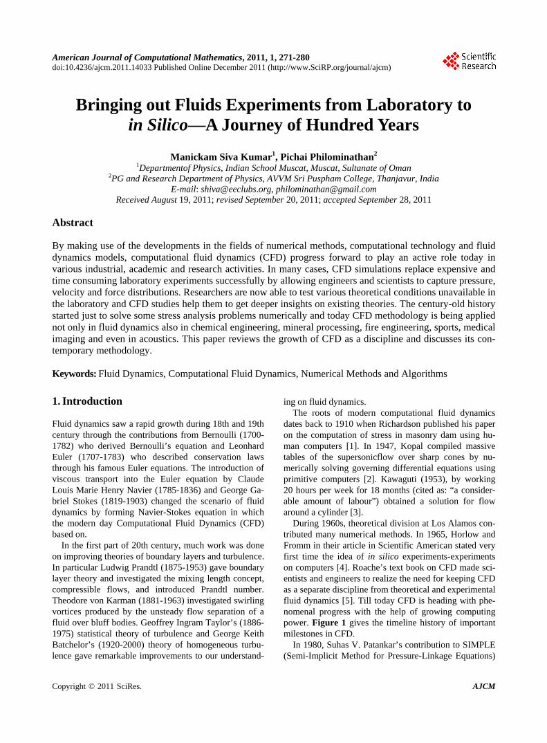
During 1960s, theoretical division at Los Alamos con-tributed many numerical methods. In 1965, Horlow and Fromm in their article in Scientific American stated very first time the idea of in silico experiments-experiments on computers [4]. Roache’s text book on CFD made sci-entists and engineers to realize the need for keeping CFD as a separate discipline from theoretical and experimental fluid dynamics [5]. Till today CFD is heading with phe-nomenal progress with the help of growing computing power. Figure 1 gives the timeline history of important milestones in CFD.
In 1980, Suhas V. Patankar’s contribution to SIMPLE Semi-Implicit Method for Pressure-Linkage Equations) (
Figure 1. Some important milestones in CFD. algorithm and his ground breaking CFD book Numerical Heat Transfer and Fluid Flow [6], made him one of the most cited authors in science and engineering [7].1980’s and 1990’s saw a revolutionary change in CFD—the availability of commercial CFD codes removed the prac-tice of writing program to perform CFD calculations.
Today, CFD is considered as a better alternative for experimental investigation to test theoretical conditions unavailable in the laboratory and to examine prototyping, optimizing design and checking industry compliance etc. [8]. In particular, the reasons for growing importance to CFD in the field of engineering can be attributed to:
1) Quick forecast of performance; 2) Better alternative to costly and impossible experi-
ments; 3) Better insights unlike experiments with expensive
probes/sensors; 4) Availability of faster computational speed and lar-
ger memory size. This paper reviews CFD in the historical perspective
pertaining to laminar flow. As the body of literature is very vast in this field, the application of CFD to thermal, electromagnetic, acoustic and other fields was not taken
into account in this work.
2. The Overview of Present CFD Methodology
The present approach to CFD methodology is to consider it as a numerical experiment which is modeled using go- verning equations and observed through running a cho-sen algorithm [8]. The final step, similar to any conven-tional fluids experiment, is to interpret results and ana-lyze (Figure 2).
In continuum mechanics non-conservation form of equations governing fluid’s kinetic energy (K), internal energy (U), mechanical power (M) and heat energy (Q) can be written as[9],
K U + M + Q
D D
Dt Dt (1)
The conservation form of equations, so-called Na-vier-Stokes equations, is given in terms of conservation flow variables (U), convection flux variables (Fi), diffu-sion flux variables (Gi) and source terms (B) is given by [9],
M. S. KUMAR ET AL. 273
i i
i it x x
F GU
B (2)
CFD involves converting these partial differential equations into discretized algebraic equations. These set of equations are numerically solved at a given point/time to get flow parameters. Any complex geometry of the flow can be converted into grid or mesh with discrete points where the flow variables are solved. Using appro-priate interpolation schemes, flow variables are obtained at non-grid point locations also. The following flow chart (Figure 3) details the steps involved in the contemporary CFD methodology [10].
3. Discretization
The literature on discretization methods is huge and ex-tensive and therefore the most common discretization methods that are important for CFD,are discussed briefly in this section.
The governing partial differential equations are con-verted into a set of algebraic equations using the discre-
Figure 2. Fluids experiment versus CFD studies.
Figure 3. The contemporary CFD methodology.
tization process (Figure 4) which describes continues flow field in terms of discrete values at prescribed loca-tions. Discretization offers the following advantages over continuum: infinite unknowns become finite, analytical approach is converted into numerical, applicability is widened and approximation becomes possible.
3.1. Finite Difference Method (FDM)
Finite Difference Method is based upon the differential form of the PDE to be solved and it employs global mapping of geometry. It is one of the oldest discretiza-tion schemes [1]. Thom (1933) gave the first ever nu-merical solution for flow over a circular cylinder [11]. This methodology involves the following steps (Figure 5(a)):
1) The infinite set of points is replaced by finite set of points called nodes.
2) Navier-Stokes equations are enforced at these nodes.
3) Differential equation converted into stencils at mesh nodes.
4) Stencils relate velocity and pressure values FDM is easy to implement in CFD analysis and pro-
vides discrete solution. But it is restricted to simple grids and does not conserve momentum, energy, and mass on coarse grids. Higher order FDM is hard to be locally conservative.Modern FDM codes make use of overlap-ping grids, where the solution is interpolated across each grid.
3.2. Finite Element Method (FEM)
Finite Element Method is based upon an integral form of the PDE to be solved and it uses local geometric map-ping. Though Courant (1943) applied this method to solve torsion problem, the name was given by Clough in 1960 [12]. For analyzing structural mechanics problems, this method was refined greatly in 60’s and 70’s and ap-plied for fluid flow in late 70’s. This methodology pro-vides a continuous solution up to a point with local ap-proach. The steps involved are (Figure 5(b)):
1) The flow field is represented as large number of known functions;
2) By using Navier-Stokes equations, the one with the best approximation properties is selected;
3) The domain is divided into elements in which the candidate functions are constructed from interpolation functions;
4) The value of the function at the nodes determines the value of the function everywhere inside the element;
5) The mesh is formed by combining all the elements. The main advantage of this method in CFD point view
is high adaptability and accuracy on coarse grids. FEM is excellent for diffusion dominated problems, viscous and free surface problems. But FEM cannot handle fluid me- chanics equations effectively and therefore this method has limited accuracy, slow for large problems and not well suited for turbulent flow.
3.3. Finite Volume Method (FVM)
Finite Volume Method is based upon a piecewise repre-
sentation of the solution in terms of specified basis func-tions. Evans & Harlow (1957) well documented the first use [13]. During late 70’s body fitted grids and early 90’s unstructured grid methods had appeared. FVM is con-sidered as integral version of FDM and can be derived also from FEM [8]. This methodology involves the fol-lowing steps to be followed (Figure 5(c)):
1) The volume of the fluid is divided into a finite num-ber of volumes, or cells;
2) Navier-Stokes equations are converted into equiva-lent integral form and applied to each cell;
3) The local form of the governing equations balances mass and momentum fluxes across the faces of each in-dividual cell.
There are efficient and well developed solvers are available using FEM, though it is applicable on coarse grids, there are issues like false diffusion, difficult stabil-ity and convergence analysis.
3.4. Other Methods
Boundary Element Method (BEM) is used for potential flows where the integrals over the whole domain are transformed over the boundaries [14,15]. This method is also called as panel method since each element plays the role of a panel on the surface of airfoil. BEM requires less data, less time and since discretization takes place on the surface, system of equations are smaller. BEM is effective for external flows such as potential and stokes flows. At the same time, this method is not good for non-linear flow problems and involves complex mathe-matics different from other CFD schemes.
Coupled Eulerian-Lagrangian (CEL) method is an-other method used widely in CFD. In the case of moving mesh points along with the fluid particles, Lagrangian coordinates have to be used in computing variables. Therefore it is convenient to have both Eulerian and La-grangian coordinates coupled, called as the CEL method [8]. This method combines advantages of both Eulerian and Lagrangian methods and useful in highly distorted and multiphase flows. But heat transfer analysis is lim-ited and mass scaling is not supported. Due to approxi-mations, the corners of solids are rounded.
The modern Spectral Methods (SM) was first pro-posed by Gottlieb and Orszag [16]. This method involves multi-dimensional discretization which is formulated as tensor products of one-dimensional constructs in or-thogonal simply-connected domains. Such methods are broadly classified as collocation methods and Galerkin methods. Sun et al. (2006) proposed another improvised method combining with finite volume, called spectral finite volume method for 3D space [17]. It takes a global approach and has exponential convergence which leads
M. S. KUMAR ET AL. 275 to high accuracy CFD analysis. But it can handle only simple geometries and applicable for limited boundary conditions. Huynh (2007) has extended spectral method using flux reconstruction approach and applied to high- order schemes successfully [18].
Unlike other methods, Lattice Boltzmann Methods (LBM) models the fluid consisting of fictive particles [18]. It makes use of particles on hexagonal grids where particles move according to discrete rules. The macro-scopic motion of the particles resembles the Navier- Stokes equation. This method is efficient in handling with complex boundaries, microscopic interaction and parallelization of the algorithm [19]. But its main disad-vantage is rrequirement of higher order terms in solving compressible flows and coupling density to temperature variations.
The smoothed particle hydrodynamics (SPH) makes use of mesh-free method and involves modeling fluid as particles and smoothening them using kernel function [19]. This method is capable of simulating flow in real time, but its limitation includes requirement of large number of particles for better resolution.
For fine grids each type of method gives the same so-lution. But some methods are more suitable to specific cases than others and the preference is determined by the attitude of the developer [10].
4. Meshing
Grid or mesh is a discrete representation of the geometric domain where problem is to be solved. Mesh divides the solution domain into subdomains like nodes, elements and control volumes.Since from the first attempt of ob-taining numerical solutions to partial differential equa-tions, the concept of mesh generation has been associated with computational methods [20]. Slowly mesh genera-tion steadily evolved as a separate discipline drawing on ideas from mathematics and computer science. In 1950’s FDM was put into use through two dimensional simple boundary shapes. By using coordinate transformations mesh that is aligned with boundaries was in use [21].
Due to the development of FEM which involved com-plex boundaries, manual mesh creation was used during late fifties and early sixties [22]. In order to apply FDM for their calculations, CFD community started using me- shes with simple generic shapes like a rectangle or circle to represent complex geometry [23]. Since then CFD became key drivers in simulating the development of various mesh generating techniques. Though FEM is powerful and versatile, the quality of mesh can greatly affect the accuracy of result. Manual generation of high quality mesh is time consuming and error-prone. It is important to note that the appropriate type of mesh and
its resolution is problem dependent. Various mesh strategies were in use during the last
few decades. For example, in 70’s algebraic methods, 80’s multiblock types and 90’s composite and overset methods were used for generating mesh. Thereare large number of types of mesh available as of today (Figure 6).
In order to generate various types of mesh, there are large number of methods available. Some of them in-clude: mesh topology first (mesh smoothing [24]), nodes first (topology decomposition, node connection [25]), adapted mesh template (grid-based [26], mapped element [27], conformal mapping [28]) and simultaneous nodes and elements approach (geometry decomposition [29]).
The mesh generation itself is becoming a separate dis-cipline and more detailed methods of mesh generation can be found in various dedicated texts [30-32]. It is also important to note now-a-days CFD users have a choice of number of mesh generating software such as Gambit from Ansys (www.ansys.com), Gridgen from Pointwise (www.pointwise.com) and Gridpro from PDC (www.gridpro.com). At the same time, many commercial CFD applications have built-in and user-friendly mesh generators. (e.g.: Solidworks flow simulation from DSS inc. (www.solidworks.com), Flow-3D from Flowscience (www.flow3d.com) etc).
5. Boundary Conditions
While solving the Navier-Stokes and continuity equa-tions, boundary conditions need to be applied. Boundary conditions for fluid flow are generally complicated due to coupling of velocity fields with pressure distribution. Incorrect, over or under boundary condition will lead to wrong results.
In CFD analysis there are two types of requirements regarding boundary conditions. Some variables will take
a constant value at the boundary (Dirichlet condition) while some variable may have constant gradients (Neu-mann conditions). In one dimensions, as FEM, FDM and FVM provide identical final algebraic equations, there-fore Dirichlet boundary conditions will give same results for all these methods [8]. Neumann boundary conditions are approximated before applying in FDM, but applied exactly in FEM and FVM.We can also apply mixture of Dirichlet and Neumann as a boundary condition. It im-portant to note that at a given boundary, different variables may be prescribed with different boundary conditions.
The general boundary conditions used in CFD studies include pressure inlet and outlet, velocity inlet and out-flow conditions. Compressible flows boundary condi-tions include mass flow inlet and pressure far-field. In addition with these there are special boundary conditions like inlet/outlet vent, intake/exhaust fan etc. Many com-mercial solvers allow users to set boundary conditions easily (Figure 7).
Wall boundary conditions are applied while using bound fluid and solid regions. In viscous flows, no slip (tangential velocity is equal to wall velocity and normal velocity is zero) conditions are usually applied. For tur-bulent flows, wall shear stress and wall roughness can be defined. For moving wall boundary conditions sliding or moving mesh techniques are used [10].
In the case of symmetric flow field and geometry, us-age of symmetry boundary conditions reduces computa-tional effort during CFD simulation. No inputs for these boundary conditions are required but one has to define boundary locationscorrectly. Such boundary conditions are used in modelling slip walls in viscous flow. In case of periodically repeating flow pattern, periodic bounda-ries reduce computational load in CFD simulations.
6. CFD Solvers
The process of discretization finally brings out set of
coupled algebraic equations which may be linear or non-linear. Irrespective of the method of discretization these equations should be solved for a discrete solution using direct or iterative methodologies. Direct methods make use of standard methods of linear algebra. Matrix methods are employed in order to devise efficient solu-tion techniques. Iterative methods involve guess-and- correct methodology till solution is converged. One of the simplest iterative methods is Jacobi method involving matrix diagonlization. Gauss-Seidel method or Liebmann method is twice as fast as the Jacobi method, makes use of successive displacements in solving set of linear equa-tions. But owing to slow convergence, they are not used in practice.
In any typical present day CFD simulations, there are multi-dimensions with larger number of grid points. There- fore both Jacobi and Gauss-Seidel becomes ineffective and expensive. Peaceman and Rachford (1955) proposed Alternating Direct Implicit (ADI) method which consid-ers multidimensional problem as a set of low dimen-sional problems [33]. Stone (1968) proposed Strongly Implicit Procedure (SIP) which involves matrix appro- ximation and Lower-Upper factorization [34]. This is used in some commercial CFD codes to solve non-linear equations in the case of multigrid methods.
Patankar and Spalding (1972) proposed a class of it-erative methods called Semi-Implicit Method for Pres-sure-Linkage Equations (SIMPLE) for coupling pres-sure-velocity for an incompressible flow [35]. This is available today in almost all commercial codes (Figure 8). Followed by this, Van Doormal and Raithby (1984) proposed SIMPLEC (SIMPLE-Consistent) which omits less significant terms in velocity correction equation [36]. Issa (1986) proposed Pressure Implicit with Splitting of Operators (PISO) algorithm, which involves an addi-tional pressure correction equation for speedy conver-gence [37]. These solvers are readily available for the users in various commercial CFD software (Figure 9).
At the same time, multigrid methods offer fastest nu-merical algorithms for solving systems of equations [38]. Geometric multigrid methods offer optimal scaling and memory cost, but highly depending on geometric infor-mation with trouble in plug-in black-box. Based on same principle, algebraic methods have been proposed with is robust and ideal without any other information. Unlike other methods, this is abstract, complex and involving repeat overhead costs.
Saad and Schultz have developed general minimum residual method (GMRES) algorithm to solve nonsym- metric linear system of equations [39]. This algorithm is capable of non-linear scaling and preconditioning for better performance. It is now considered as very robust, memory intensive and easy to parallelize therefore used widely in many commercial codes.
Irrespective of the procedures used, the solutions ob-tained should be accurate (free from modelling and trun-cation errors), consistent (to ensure refines mesh/time
step yield more accurate results) and stable (single, mesh independent solution).
7. Post-Processing
The output of computational results of CFD study is usu-ally colourful and vivid. Usually almost all CFD study results are presented graphically through one of the fol-lowing categories:
1) XY plots (time/iterative history of residuals and forces); 2) 2D/3D contour plots (dynamic-, absolute-, and to-
Q criterion etc.); 5) Streamlines, pathlines and streaklines etc; 6) Animations. Various techniques have been used to analyse and
visualize the fluid parameters of the study. Early visuali-zations made use of glyphs to represent vector fields in the data [40]. Later, line integral convolution (LIC) and texture based approaches [41] were used to depict realis-tic flow. Feature based visualization were also used on extracted features directly to analyse flow data. Accurate core feature detection algorithms [42] were widely used in many commercial codes. During post processing de-rived variables (vorticity, shear stress etc.) integral vari-ables (forces, lift/drag coefficients) and turbulent quanti-ties (Reynolds stresses, energy spectra) are calculated. Figure 10 shows a typical post processed results using CFD methodology [43].
Almost all commercial CFD applications have their built-in GUI visualization tools. In addition with them there are some standalone CFD visualisation tools like FIELDVIEW (ilight.com), TECPLOT (amtec.com), and ENSIGHT (ceintl.com) are available today. GNUPLOT (gnuplot.info) is another open-source popular plotting package in CFD industry.
8. Conclusions
The application domain of CFD is widening with the advancement with accurate numerical methods, compu-tational models and visualisation techniques. CFD that was just meant for fluid dynamics, now it is used as re-search tool (to test theoretical advances unavailable in the lab), educational tool (to teach thermal and fluid sci-ences), design optimization tool (in aerospace and auto-mobile industry). It has been also extended in studying chemical, mineral processing and civil, environmental engineering, power generation and even sports.
With the exorbitant growth of computer simulation technology, CFD is evolving rapidly with more tech-
Figure 10. Top: flow trajectories past sphere at Reynolds number 150. Bottom: post processed results showing velocity con-tours across a cross-section of a rotating solid helix in viscous fluid at zero Reynolds number [43].
[3] Z. Kopal, “Tables of Supersonic Flow around Cones,” Department of Electrical Engineering Cambridge, Center of Analysis, Massachusetts Institute of Technology, 1947.
niques and models. Complex fluid mechanical problems such as buoyant fires, jet flames, multiphase flows are progressively handled by todays CFD technology. De-creasing hardware costs and increasing processor speeds challenge CFD developers to help in what is called zero prototype engineering.
[4] T. J. Chung, “Computational Fluid Dynamics,” Cam- bridge University Press, Cambridge, 2002. doi:10.1017/CBO9780511606205
[5] A. Thom, “The Flow Past Circular Cylinders at Low Speeds,” Proceedings of the Royal Society of London. Series A, Vol. 141, No. 845, 1933, pp. 651-666. doi:10.1098/rspa.1933.0146
9. References
[1] R. Courant, K. Friedrichs and H. Lewy, “Uber die Partiel- lendifferenzgleichungen der Mathematischen Physik,” Ma- thematische Annalen, Vol. 100, No. 1, 1928, pp. 32-74. doi:10.1007/BF01448839
[6] M. Kawaguti, “Numerical Solution of the NS Equations for the Flow around a Circular Cylinder at Reynolds Num- ber 40,” Journal of Physical Society of Japan, Vol. 8, No. , 1953, pp. 747-757. doi:10.1143/JPSJ.8.747
[2] L. F. Richardson, “The Approximate Arithmetical Solu- tion by Finite Differences of Physical Problems Involving Differential Equations with an Application to the Stresses in Masonry Dam,” Philosophical Transactions of the Royal Society of London. Series A, Vol. 210, No. 459-470, 1910, pp. 307-357.
[7] S. V. Patankar, “Numerical Heat Transfer and Fluid Flow,” Hemisphere Publishing Corp., Washington DC, 1980.
[8] R. P. Loui, “Top 100 Hits,” 2008. (cited 2 October 2011). http://www.cse.wustl.edu/~loui/goocites.html
[9] D. Gottlieb and S. A. Orszag, “Numerical Analysis of Spec-
tral Methods: Theory and Applications Pennsylvania,” SIAM, Philadelphia, 1993.
[10] J. G. Zhou, “Lattice Boltzmann Methods for Shallow Water Flows Newyork,” Springer, Berlin, 2004.
[11] J. H. Ferziger and M. Peric, “Computational Methods for Fluid Dynamics,” Springer, Berlin, 2002. doi:10.1007/978-3-642-56026-2
[12] C. Sells, “Plane Subcritical Flow Past a Lifting Aerofoil,” Proceedings of the Royal Society of London. Series A, Vol. 308, No. 1494, 1968, pp. 377-401.
[13] T. J. Baker, “Mesh Generation: Art or Science?” Progress in Aerospace Sciences, Vol. 41, No. 1, 2005, pp. 29-63. doi:10.1016/j.paerosci.2005.02.002
[14] A. Denayer, “Automatic Generation of Finite Element Meshes,” Computers & Structures, Vol. 9, No. 4, 1978, pp. 359-364.
[15] Wordenweber, “Volume Triangulation,” CAD Group Do- cument No. 110, University of Cambridge, Cambridge, 1980.
[16] W. C. Thacker, A. Gonzalez and G. E. Putland, “A Me- thod for Automating the Construction of Irregular Com- putational Grids for Storm Surge Forecaste Models,” Journal of Computational Physics, Vol. 37, No. 3, 1980, pp. 371-387. doi:10.1016/0021-9991(80)90043-1
[17] S. F. Yeung and M. B. Hsu, “A Mesh Generation Method Based on Set Theory,” Computers & Structures, Vol. 3, No. 5, 1973, pp. 1063-1077. doi:10.1016/0045-7949(73)90038-2
[18] W. Barfield, “Numerical Method for Generating Ortho- gonal Curvilinear Meshes,” Journal of Computational Phy- sics, Vol. 5, No. 1, 1970, pp. 23-33. doi:10.1016/0021-9991(70)90050-1
[19] A. Bykat, “Design of a Recursive, Shape Controlling Mesh Generator,” International Journal for Numerical Methods in Engineering, Vol. 19, No. 9, 1983, pp. 1375-390. doi:10.1002/nme.1620190907
[20] J. E. Thompson, Z. U. A. Warsi and C. W. Mastin, “Nu- merical Grid Generation-Foundations and Applications,” Elsevier, New York, 1985.
[21] A. S. Arcilla, J. Häuser, P. R. Eiseman and J. E. Thompson, “Numerical Grid Generation in Computational Fluid Dy- namics and Related Fields,” North-Holland, Amsterdam, 1991.
[22] V. D. Liseikin, “Grid Generation Ethods,” Springer-Ver- lag, Berlin, 1999.
[23] S. V. Patankar and D. B. Spalding, “A Calculation Proce- dure for Heat, Mass and Momentum Transfer in Three- Dimensional Parabolic Flows,” International Journal of Heat and Mass Transfer, Vol. 15, No. 10, 1972, pp. 1787-1805. doi:10.1016/0017-9310(72)90054-3
[24] J. P.V. Doormaal and G. D. Raithby, “Enhancements of the SIMPLE Method for Predicting Incompressible Flow Problems,” Numerical Heat Transfer, Vol. 7, No. 2, 1984, pp. 147-163.
[25] D. W. Peaceman and H. H. J. Rachford, “The Numerical Solution of Parabolic and Elliptic Differential Equations,” Journal of Society for Industrial and Applied Mathemat-
ics, Vol. 3, No. 1, 1955, pp. 28-41. doi:10.1137/0103003
[26] H. L. Stone, “Iterative Solution of Implicit Approxima- tions of Multidimensional Partial Differential Equations,” SIAM Journal on Numerical Analysis, Vol. 5, No. 3, 1968, pp. 530-558. doi:10.1137/0705044
[27] R. I. Issa, “Solution of the Implicitly Discretised Fluid Flow Equations by Operator-Splitting,” Journal of Com- putational Physics, Vol. 62, No. 1, 1986, pp. 40-65. doi:10.1016/0021-9991(86)90099-9
[28] Y. Saad and M. H. Schultz, “GMRES: A Generalized Minimal Residual Algorithm for Solving Nonsymmetric Linear Systems,” SIAM Journal on Scientific Computing, Vol. 7, No. 3, 1986, pp. 856-869. doi:10.1137/0907058
[29] W. Hackbusch, “Multigrid Methods and Applications- omputational Mathematics,” Springer-Verlag, Berlin, 1985.
[30] J. Argyris and P. Patton, “Computer Oriented Research in a Universitymilieu,” Applied Mechanics Reviews, Vol. 19, No. 12, 1966, pp. 1029-1039.
[31] L. Richardson, “Weather Prediction by Numerical Proc- ess,” Cambridge University Press, Cambridge, 1922.
[32] J. J. Monaghan, “An Introduction to SPH,” Computer Phy- sics Communications, Vol. 48, No. 1, 1988, pp. 88-96. doi:10.1016/0010-4655(88)90026-4
[33] B. Cabral and L. C. Leedom, “Imaging Vector Fields Us- ing Line Integral Convolution,” Proceeding of the 20th Annual Conference on Computer Graphics, Anaheim, 1993, pp. 263-270.
[34] R. S. Laramee, H. Hauser, H. Doleisch, B. Vrolijk, F. H. Post and D. Weiskopf, “The State of the Art in Flow Visualization: Dense and Texture-Based Techniques,” Com- puter Graphics Forum, Vol. 23, No. 2, 2004, pp. 143-161.
[35] F. H. Post, B. Vrolijk, H. Hauser, R. S. Laramee and H. Doleisch, “The State of the Art in Flow Visualization: Feature Extraction and Tracking,” Computer Graphics Forum, Vol. 22, No. 4, 2003, pp. 775-792. doi:10.1111/j.1467-8659.2003.00723.x
[36] F. H. Harlow and J. E. Fromm, “Computer Experiments in Fluid Dynamics,” Scientific American, Vol. 213, No. 3, 1965, pp. 104-110. doi:10.1038/scientificamerican0365-104
[37] P. J. Roache, “Computational Fluid Dynamics,” Hermosa Publications, Albuquerque, 1972.
[38] M. W. Evans and F. H. Harlow, “The Particle-in-Cell Method for Hydrodynamic Calculations,” Scientific La- boratory Report, Los Alamos, 1957.
[39] J. L. Hess, “Review of the Source Panel Technique for flow Computation,” In: R. P. Shaw, J. Periaux, A. Chau-douet, J. Wu, L. Morino and C. A. Brebbia, Eds, Proceed-ings of 4th International Symposium on Innovative Nu-merical Methods in Engineering, Atlanta, Springer-Verlag, 1986, pp. 197-210.
[40] J. L. Hess, “Panel Methods in Computational Fluid Dy- namics,” Annual Review of Fluid Mechanics, Vol. 22, No. 1, 1990, pp. 255-74. doi:10.1146/annurev.fl.22.010190.001351
[41] Y. Sun, Z. J. Wang and Y. Liu, “Spectral (Finite) Volume Method for Conservation Laws on Unstructured Grids:
[43] M. Siva Kumar and P. Philominathan, “Computational Fluid Dynamics Modeling Studies on Bacterial Flagellar Motion,” International Journal of Fluid Machinery and Systems, Vol. 4, No. 3, 2011, pp. 341-348.


![L-14 Fluids [3] Fluids at rest Fluid Statics Fluids at rest Fluid Statics Why things float Archimedes’ Principle Fluids in Motion Fluid Dynamics.](https://static.documents.pub/doc/80x56/56649ced5503460f949ba1d5/l-14-fluids-3-fluids-at-rest-fluid-statics-fluids-at-rest-fluid-statics.jpg)

![L-14 Fluids [3] Fluids at rest Why things float Archimedes’ Principle Fluids in Motion Fluid Dynamics –Hydrodynamics –Aerodynamics.](https://static.documents.pub/doc/80x56/56649d9f5503460f94a89e67/l-14-fluids-3-fluids-at-rest-why-things-float-archimedes-principle.jpg)


![L-14 Fluids [3] Why things float Fluids in Motion Fluid Dynamics –Hydrodynamics –Aerodynamics.](https://static.documents.pub/doc/80x56/56649dea5503460f94ae4fa2/l-14-fluids-3-why-things-float-fluids-in-motion-fluid-dynamics.jpg)
