This content has been downloaded from IOPscience. Please scroll down to see the full text.

Download details:

IP Address: 155.54.213.13

This content was downloaded on 02/04/2015 at 09:10

Please note that terms and conditions apply.

Bringing partial differential equations to life for students

View the table of contents for this issue, or go to the journal homepage for more

2015 Eur. J. Phys. 36 035026

(http://iopscience.iop.org/0143-0807/36/3/035026)

Home Search Collections Journals About Contact us My IOPscience

Bringing partial differential equations to lifefor students

María José Cano1, Eliseo Chacón-Vera2 andFrancisco Esquembre2

1Departamento de Matemáticas, Universidad de Murcia, Campus de Espinardo,E-30.100, Murcia, Spain2 Departamento de Informática y Automática, ETSI de Informática de la UNED,C/Juan del Rosal, 16, E-28040 Madrid, Spain

E-mail: mjcanovicente@gmail.com

Received 7 December 2014Accepted for publication 20 February 2015Published 1 April 2015

AbstractTeaching partial differential equations (PDEs) carries inherent difficulties thatan interactive visualization might help overcome in an active learning process.However, the generation of this kind of teaching material implies seriousdifficulties, mainly in terms of coding efforts. This work describes how to usean authoring tool, Easy Java Simulations, to build interactive simulationsusing FreeFem++ (Hecht F 2012 J. Numer. Math. 20 251) as a PDE solverengine. It makes possible to build simulations where students can changeparameters, the geometry and the equations themselves getting an immediatefeedback. But it is also possible for them to edit the simulations to set deeperchanges. The process is ilustrated with some basic examples. These simula-tions show PDEs in a pedagogic manner and can be tuned by no experts in thefield, teachers or students. Finally, we report a classroom experience and asurvey from the third year students in the Degree of Mathematics at theUniversity of Murcia.

Keywords: authoring tools and methods, physical modelling, improvingclassroom teaching

1. Introduction

Partial differential equations (PDEs) are a core part of the curriculum of any applied studiesnowadays. They describe all kinds of physical phenomena and applications in all sorts offields. However, teaching PDEs is a difficult task due to a number of reasons:

European Journal of Physics

Eur. J. Phys. 36 (2015) 035026 (14pp) doi:10.1088/0143-0807/36/3/035026

0143-0807/15/035026+14$33.00 © 2015 IOP Publishing Ltd Printed in the UK 1

• The equations are intrinsically a complicated matter and it is not simple to handle an easyintroduction to the field [15].

• A typical approach to this field leads to the analytic solution of the basic transport,diffusion and wave equations with constant coefficients. This is not a simple task andmight obscure the real meaning of the models at hand. Moreover, it does not lead straightaway to some meaningful imagery of the studied phenomenon [5].

• A common strategy is the separation of variables method which requires someknowledge of Fourier series. This adds more noise to the picture [15].

• Solutions are not numbers but functions, a conceptual jump for students that is betterunderstood by using graphical visualizations [18].

• Exact resolution of most of the PDEs is not possible and one has to resort to numericaltechniques, like finite differences or finite elements [18]. These tools are far beyond abasic course.

Similar difficulties are found when teaching basic physics courses, see [14] for a detailedreflection. The didactic and pedagogic implications are the permanent need for studentfeedback to detect conceptual failures and the proposal is the combination of blackboardlectures, analysis of solutions and computer lab sessions [11, 15, 19].

Particularly interesting is the concept of interactive engagement. The student interacts inreal time tuning the parameters, learning and feeling the reactions of the solutions of themodel. This is followed by exchange and discussion of ideas with peers and teacher [10].

Computer simulations give the student the opportunity to create the solution of a parti-cular equation and play with it. Through interactivity, students can predict a situation,understand the role of the different parameters and terms in an equation and have a visual ideaof the whole process. This also helps the construction of mental models away from thecomplexity of the mathematical equations, [12, 19] and [20].

As a consequence, our purpose in this work is to offer an interactive engagement of thestudent with the models via computer simulations.

There exist some tools for the resolution and visualization of PDEs. Some of themrequire a licence to be bought, like MATLAB, Mathematica or MAPLE, and others require asteep learning curve in terms of coding for students and teachers, like OpenFoam [16], Elmer[2] or FreeFem++ [6]. All of them offer restricted interaction possibilities.

Interactivity is the main asset of the simulations created with the authoring tool Easy JavaSimulations (EJS) [3], however only ordinary differential equation solvers were available inthe distribution up to this date. For this reason, we have connected this tool to a PDE solverand chosen the finite element solver FreeFem++ because it gives full control of the equationsand boundary conditions of the problem at hand.

This research has been tested in a classroom setting on the 3rd year of the mathematicsdegree at the University of Murcia. Students had a two-hour computer lab session where themost basic physical phenomena of diffusion, reaction and transport where observed andtested.

Models were classified in terms of the typical differential operators and, henceforth, theystudied the elastic membrane for the Laplace operator, the heat equation with reaction and thewave equation.

Activities were proposed for individual study with a guideline that set up the main stepsin the learning process for each model: observation, prediction and testing.

The whole process of combining EJS with FreeFem++ is introduced in section 2. Insubsections 2.1–2.4 we follow the process of building a simulation that solves and plots thesolution of a simple PDE, the Dirichlet problem for Laplace operator. On the way, we detail

Eur. J. Phys. 36 (2015) 035026 M J Cano et al

2

three fundamental aspects: definition and resolution of the equations in FreeFem++ languagefrom EJS, storage of the data and graphic visualization. The full capabilities of interactivityare shown in a complete example in subsection 2.5. In section 3 we report our results withstudents in a lab experience and present two more examples of simulations. Finally, in the lastsection we gather our conclusions.

2. Materials and methods

2.1. A few words on FreeFem++: script construction

FreeFem++ is a C++-like computer language dedicated to the finite element method. It isdeveloped and maintained by Frédéric Hecht from the Jacques–Louis Lions Laboratory at theUniversity of Pierre et Marie Curie in Paris. This language gives total control on the PDEproblem and nowadays there exists a very active community of users. For documentation andexamples we refer the reader to the web sites [6] and wiki [7]. In the following, we give thebasic commands that are needed to describe our Dirichlet problem.

A PDE gives the evolution in time and space of a quantity in a region of interest. Thisregion could be defined by the parametric description of its boundary. For example, asquare is

border a(t=0,1){x=t; y=0; label=1;};border b(t=0,1){x=1; y=t; label=2;};border c(t=1,0){x=t; y=1; label=3;};border d(t=1,0){x=0; y=t; label=4;};

Next, a triangulation is generated on this domain and it is determined by arbitrary intervalpartitions on each boundary border like this:

mesh Th buildmesh a 20 b 30 c 10 d 40= + + +( ( ) ( ) ( ) ( ));

Freefem++ also includes some shortcuts to generate the most common domains. It is the caseof

mesh Th square 20 20= ( , );

which determines a 20 × 20 uniform triangulation on the unit square domain.For our example problem we will take the computational domain Ω = ×(0, 1) (0, 1)

with boundary ∪ ∪ ∪δΩ Γ Γ Γ Γ= 1 2 3 4 and a triangulation as described above. Our fullproblem for the Laplace operator with Dirichlet boundary conditions is

∪ ∪ΩΓ Γ ΓΓ

−△ ===

u fu

u

, in ,0, on ,1, on .

(1)1 2 3

4

⎧⎨⎪⎩⎪

In FreeFem++ PDEs must be written in variational form: find ∈u V such that

∫ ∫= ∀ ∈Ω Ω

u v fv v V· , , (2)

where V is a proper function space [1]. Then, the full FreeFem++ script is

Eur. J. Phys. 36 (2015) 035026 M J Cano et al

3

mesh Th square 20 20 triangulationfespace Vh Th P1 P1 finite elementsVh u v two functions from Vh spacefunc f 0 expression for function fproblem laplace u v

bilineal part from 2int2d Th dx u dx v dy u dy vright side from 2int2d Th f vDirichlet boundary conditionon 1 2 3 u 0 on 4 u 1

laplace solves PDEplot u visualizes the solution

++=

==

+

+ −

+ = + =

Listing 1. Simple FreeFem script.( , ); //

( , ); //, ; //

; //( , )

// ( )( )( ( )* ( ) ( )* ( ))

// ( )( )( * )

//( , , , ) ( , );

; //( ); //

A front end user might work with FreeFem++ in two manners: either in terminal mode orby using the integrated environment FreeFem++-cs [13], written by Antoine Le Hyaric. Thissecond version also allows a remote TCP-IP connection with another computer or a highperformance server.

2.2. A few words on Easy Java Simulations

We choose Easy Java Simulations [4] because it meets all the requirements for an interactiveengagement methodology. This open-source tool allows the generation of interactive simu-lations in a simple way and it was developed with an emphasis in teaching versatility. Theuser can change parameters and other aspects of these simulations and get a real-timevisualization of the results.

Usually, an interactivity like that is obtained after a complicated coding process. A highprogramming level is needed to create the view and graphical interface and it hinders changes.This is not the case with EJS, to begin with, the teacher can supply students with closedsimulations as applets with an interface that allows some changes in the model. Once studentsare familiar with the simulation they could read the code inside thanks to the modularconception of the software.

Each simulation consists of three stages and each one has a different panel window:description, model and view.

The description panel is basically an HTML editor that permits the creation of one ormore tabs of information about the simulation. Besides a description of the model, it ispossible to add activities and questions that help on its use.

The model panel, figure 1, is the central point of the simulation. It is subdivided into sixsubpanels where the model is implemented in a guided and structured way. We brieflydescribe them now.

• Variables subpanel takes care of the variables by means of a menu where, for eachvariable, we give name, initial value and type.

• Initialization subpanel might include, if needed, lines of code to set up these variables.• Evolution subpanel might include lines of code to set up ordinary differential equationsor any other model.

• Fixed relations subpanel stores pieces of code to be run on each step.

Eur. J. Phys. 36 (2015) 035026 M J Cano et al

4

• Custom subpanel might include functions defined by the user to be called from otherparts of the simulation.

• Elements is the final and more interesting subpanel. These elements serve to connect EJSwith other libraries and allow external contributions to EJS.

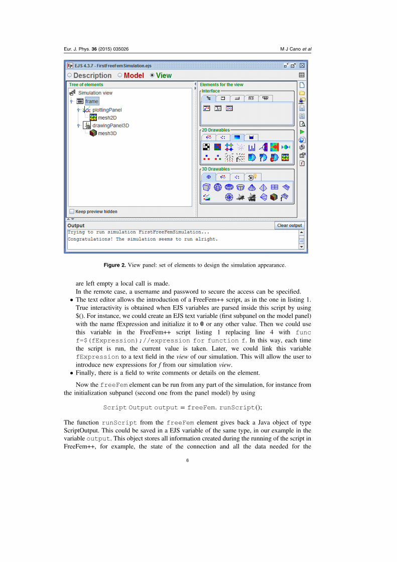
The panel view, figure 2, allows the construction of a graphical interface from a largevariety of elements included in EJS just by a drag and drop process.

The connection of FreeFem++ with EJS has been made working on the subpanel ele-ments and the panel view. These modifications are described in the next two subsections.

2.3. The FreeFem++ element in EJS

In the subpanel elements we have the connection with FreeFem++. Inside elements there aredifferent folders containing all the elements. In particular, in the external folder the FreeFemicon is found. Adding a new element to the simulation is made by a drag-and-drop process ofthe FreeFem icon to the list of elements on the left-hand side of the window, figure 3.

The properties of this element, and of any other, can be changed by a double click on it,see the bottom-left of figure 3. In this way, a property menu is displayed with three parts.

• The first group has three text fields that set up the connection with the computer that runsFreeFem++. This connection can be local or remote. To connect with a remote server it isnecessary to give the URL address on the corresponding field. Otherwise, when the fields

Figure 1. Model panel: view of subpanel variables, first of six subpanels to define theproblem.

Eur. J. Phys. 36 (2015) 035026 M J Cano et al

5

are left empty a local call is made.In the remote case, a username and password to secure the access can be specified.

• The text editor allows the introduction of a FreeFem++ script, as in the one in listing 1.True interactivity is obtained when EJS variables are parsed inside this script by using$(). For instance, we could create an EJS text variable (first subpanel on the model panel)with the name fExpression and initialize it to 0 or any other value. Then we could usethis variable in the FreeFem++ script listing 1 replacing line 4 with funcf=$(fExpression);//expression for function f. In this way, each timethe script is run, the current value is taken. Later, we could link this variablefExpression to a text field in the view of our simulation. This will allow the user tointroduce new expressions for f from our simulation view.

• Finally, there is a field to write comments or details on the element.

Now the freeFem element can be run from any part of the simulation, for instance fromthe initialization subpanel (second one from the panel model) by using

Script Output output freeFem runScript= . ();

The function runScript from the freeFem element gives back a Java object of typeScriptOutput. This could be saved in a EJS variable of the same type, in our example in thevariable output. This object stores all information created during the running of the script inFreeFem++, for example, the state of the connection and all the data needed for the

Figure 2. View panel: set of elements to design the simulation appearance.

Eur. J. Phys. 36 (2015) 035026 M J Cano et al

6

visualization of the functions and objects inserted inside a function plot from the FreeFemscript.

This information has been encapsulated in Java objects to ease their access and use inother places in the simulations, like from the initialization, evolution or even from the viewpanel.

In this way, each ScriptOutput object has a list of objects of the type PlotOutput, one foreach order plot in the script. Each one of these PlotOutput could even contain one or moreparts of a graphical output, in the form of PDEData objects. Each PDEData is a triangulationor a solution.

To obtain the graphs stored in our variable output we have to read each of thePDEData inside; for this purpose we use the function getData:

PDEDatamyPDEData output getData plotNum dataNum= . ( , );

Here plotNum will be an integer that points to each plot of the script, the first onestarting from 0. The parameter dataNum will be another integer value that gives the placethat the triangulation or the solution has in the list of arguments for the selected plot; thesearguments are also ordered from 0.

Figure 3. FreeFem element in EJS.

Eur. J. Phys. 36 (2015) 035026 M J Cano et al

7

Finally, we include in the panel initialization the following lines:

output freeFem runScriptsolution output getData 0 0

==

. ();. ( , );

In this way the solution of our problem is available everywhere in the variable solution oftype PDEData.

2.4. Visualization in EJS

According to panel view figure 2, we describe now the way the visualization is constructed.The right-hand side has three groups of icons. These icons are the view elements which serveto instantiate different view Java objects in a simple way. The first group includes windows,containers and others elements to design the interface, the second group has a large variety ofobjects to make plots and graphics in two dimensions and, finally, the third group has 3Dgraphic elements. To include a new element in our simulation the icon is selected by a singleclick and added to the view tree on the left-hand side.

The code inside some of these elements comes from the visualization library in OpenSource Physics [17].

Bearing in mind that simplicity and versatility are the main principles in EJS, we haveincluded two new view elements that simplify the visualization of triangulations and solutionsin our simulations. They are called Mesh2D and Mesh3D and are marked in figure 4.

The data to plot is inserted in the Data field of the property menu of these two newelements by using the name of the PDEData variable obtained after the FreeFem++ com-putation. Although this process can also be made by using Java variables with the convenientdata. Our software will plot the mesh of the problem and the contour line view of the solution.

To finish our simulation we use some of the view elements as follows:

(1) Add a Frame element.(2) Add a DrawingPanel3D and a PlottingPanel to this Frame (according to the screen

resolution it could be necessary to enlarge the Frame in the preview window of EJS toshow both panels).

(3) Add the Mesh2D element to the PlottingPanel (this yields the 2D view of the solution).(4) Add the Mesh3D element to the DrawingPanel3D (this yields the 3D view of the

solution).

The tree of elements in the view panel would look as in figure 2 and the resultingsimulation is shown in figure 5.

For a better understanding of the different values in the contour line plot, a legend can beattached (show legend option in the property menu) which match the colour and the solutionvalue. Furthermore, an advanced configuration of the colour allows one to set the number oflevels (levels) and the colour under and above this range (floor colour and ceil colour).

Figure 4. Row-wise view of second and third groups of icons on left side of panel view.The new ad hoc icons are marked.

Eur. J. Phys. 36 (2015) 035026 M J Cano et al

8

The autoscale option equally distribute the different levels between the minimum andmaximum values of the solution. In this way, even if the solution changes, all the range ofcolours are used. If we want to state a fixed relation between values and colours, then theoption AutoscaleZ must be set to false.

Finally, some numeric or text fields or even sliders could be added to the interface (fieldand TextField elements) to increase the interactivity of our simulation.

Thus far, our simple example has been concluded and our short overview of the softwarealso. In the next subsection we show an example with much greater interactivity in a moresketchy way.

2.5. A fully interactive simulation

The applet FF01_EllipticExample (download at [8]) is the sort of simulation a student mightwork with. It reproduces the behaviour of an elastic membrane totally or partially attached toa circular rigid support under the effect of a load. Solving the Laplace equation with con-venient boundary conditions we obtain the displacement of the membrane in the verticaldirection.

Let the elastic membrane be attached to Γ Ω= ∂ , the boundary of the 2D domain Ω, andsuppose that a force f x x( )d is applied on each surface element =x x xd d d1 2. Then themembrane displacement solves

Δφ Ω− =x f x( ) ( ) in .

The boundary conditions for this model could be of Dirichlet type (the membrane is totallyfixed on Γ) and of Dirichlet–Neumann type (only partially attached):

(1) Dirichlet type: in the case of a planar domain Ω, the boundary condition is

φ Γ=x( ) 0, on

and when Ω is not planar but at an elevation =z z x x( , )1 2 then the boundary condition is

φ Γ=x z( ) , on .

Figure 5. 2D view and 3D view of our first FreeFem++-EJS simulation.

Eur. J. Phys. 36 (2015) 035026 M J Cano et al

9

(2) Dirichlet–Neumann type: when one section of the membraneʼs boundary ΓN , where∪Γ Γ Γ= D N , is not attached, the variation g(x) of the displacement in the normal

direction is given by

φ φ Γ∂∂ ⃗

= ⃗′ ⃗ =n

x n x g x( ) · ( ) ( ) on N

and then the full set of boundary conditions are

φ Γ φ Γ= ∂∂ ⃗

=x zn

x g x( ) on , ( ) ( ) on .D N

The boundary condition on ΓN is called of Neumann type, and we require Γ ≠ ∅D for theproblem to be well posed.

2.5.1. Playing the simulation. By default initially the simulation shows the solution to theproblem

Δφ Ωφ Γ

− = −=

xx

( ) 6, in ,( ) 0, on ,

calculated on a mesh generated from a discretization over the boundary by using 30 uniformlydistributed points. In figure 6 you see the computational domain Ω with its discretization andthe 2D and 3D view of the solution. This solution is shown in a contour line plot and adifferent colour is assigned to each of these values (from the highest value in red to the lowestin blue). Check the legend in a different window (figure 7) to see the correspondence.

The top of the simulation is divided in three subpanels that allow one to modify theoriginal setting of the problem:

(1.) Domain: left panel.(2.) Equation: central panel.(3.) Boundary conditions: right panel.

2.5.2. User interaction.

(1) Changes on the view: the viewpoint of the 3D plot can be changed using the mousepointer. Also it is possible to zoom by pressing the Shift key at the same time the mouseis clicking and dragging.(a) Changes on the domain:(b) Shape and size: in the left panel the boundary of the domain Ω is described as a level

set equation. There we can change the size and shape of the domain going from acircle to an ellipse by just changing the length of the blue arrows. Also by setting adifferent numerical value in the fields labelled as axes A and B. The field is filled inyellow until the intro key is pressed and the change is applied only then.

(c) Discretization: this is set by a uniform partition of the boundary. The number ofpoints is set by the numeric field points and the larger this value the more accurate thecomputed solution is.

(2) Changes on the equations: a different expression to function =f f x y( , ) can be given inthe central panel field. Some examples of correct analytical expressions are:

2 x x y sin x y 4 sin 2 pi x y x y+ − + …* , * , ( ), * ( * * * ), ,2 2

Eur. J. Phys. 36 (2015) 035026 M J Cano et al

10

(3) Changes on the boundary conditions: initially the simulations solve the problem withhomogenous Dirichlet boundary conditions. This can be changed to a non-homogenousDirichlet conditions in the field for ΓD. Using the slider we can set a portion of theboundary as ΓN then a new field to give the Neumann boundary condition appears.

3. Results

Traditionally the subject of PDEs imparted in the mathematics degree at the University ofMurcia, has been carried out by theoretical lectures and solving some problem sets. Last year,we designed a two-hour long computer lab session to introduce this software.

3.1. Getting started

Simulations were available in a web site in two versions: the first to be run with a localFreeFem++ and the second on a multicore remote server.

As the interaction with all of the simulations is quite similar, students were introducedfirst to the use of numerical fields, sliders and how to zoom and rotate the graphics.

We worked on the three paradigmatic models: diffusion, transport and wave motion.Students previously had detailed documentation with a description of the models and some

Figure 6. Solution of Δφ− = −6 with φ = 0 at its boundary. 30 points discretizationover the boundary Ω.

Figure 7. Legend shows the correspondence between colours and the value of thecomputed solution.

Eur. J. Phys. 36 (2015) 035026 M J Cano et al

11

activities were proposed. A first set of questions offered the opportunity to get familiar withboth simulation and models, while the following ones were focused on making conjectures onchanges in the model and checking them with the simulation. Finally, some more difficultquestions, where a higher abstraction level was needed, were posed.

3.2. Simulations and activities

The first simulation was the one we presented before in section 2.5 and we succinctly describenow the other two simulations (download at [8]):

FF03_Convection_Diffusion: simulates diffusion of heat in a rectangular perforatedmetallic sheet. The initial temperature is 0 °C in all the domain. Then, a 100 °C temperature isapplied on the left-hand side and temperature flows freely towards the right-hand side whilethe other straight sides are insulated. Here the heat transmission is modelled by the diffusionoperator and the effects of transport and reaction are included.

Some of the activities proposed here were as follows.

• Identification of the type of boundary conditions applied on each piece of boundary.• Filling in a table with the time to achieve a certain temperature level on a particularportion of the block when the transport and reaction effects are null.

• Guessing the behaviour produced by an increase in the transport effect.• Studying the numerical stability of the model by using the Peclet number.• Guessing the configuration of different parameters to achieve the temperature distributionshown in a given figure.

FF04_WavesEquation: shows the vibrations of a membrane attached by its border to ahorizontal plane. Initially, the membrane is pulled from its centre to an initial position and letthen vibrate. This initial position is set by the solution of a Poisson problem.

Some of the activities proposed here were as follows.

• Studying the initial position of the membrane and the velocity of the wave propagationdepending on the parameters values.

• Detection of the loss of precision due to the iterative calculation of the numericalsolution.

Figure 8. Questions marks on the session development, visualization and interactivityof the simulations.

Eur. J. Phys. 36 (2015) 035026 M J Cano et al

12

3.3. Session evaluation

At the end of the session a short survey was handed out to the students. They were askedabout the experience and some good marks on it were given. Our students offer their opinionabout the session, the visualization of the models, interactivity of the simulations and con-cepts acquisition. They scored from 1 to 5, being 1 ‘poor’ and 5 ‘plenty’. The results areshown in figures 8 and 9.

To summarize, students positively qualified the session, pointing out:

• Positively, the simulations were easy to be played with and activities were clearly posed.• Also positively, but with a lower mark, they stated that the session had improved theirinsight into the matter.

• Visualization of the models and their interpretation were well evaluated and studentssuggested it had been crucial in their understanding.

• Interactivity with the simulations was simple and the degree of freedom wide enough.• Lower marks were given against knowledge acquisition. This might be due to thestudents’ insecurity.

• Also difficult was to associate models and the different boundary condition or thedifferent operators, the most ambitious questions in the survey.

4. Conclusions

This paper shows the design of a set of interactive simulations to teach PDEs and the result ofa practical session for an introductory course on the subject. We have built simulations for thediffusion, reaction and transport equations offering a high interactivity performance.

The building aspects of these simulations are the combination of EJS and FreeFem++softwares. Thanks to EJS, students get simple interfaces which allow interaction with themodels and, moreover, these simulations are distributed as independent applets.

The advance software FreeFem++ was used to numerically solve the equations but thisprocess can be shadowed to the students. The computational work can be done in the localcomputer of the student or in a remote server.

A complete set of activities that goes with each of the simulations guide the students tothe model. It makes them speculate about its behaviour and check the real effect of somechanges. In this way they better assimilate the physical meaning of each PDE operator.

Figure 9. Questions marks on knowledge acquisition.

Eur. J. Phys. 36 (2015) 035026 M J Cano et al

13

Acknowledgments

We thank Professor Francisco Balibrea for his collaboration in making possible the labsession. This work was partially funded by Fundación Séneca, the Regional Research Agencyof the Region of Murcia, Spain through a grant 16007/BSCE/10 and by the Spanish Gov-ernment project MTM2012-36124-C02-01.

References

[1] Allaire G 2007 Numerical Analysis and Optimization: An Introduction to Mathematical Modelingand Numerical Simulation (Oxford: Oxford University Press)

[2] www.csc.fi/english/pages/elmer (accessed July 2014)[3] Easy Java Simulations www.um.es/fem/EjsWiki/pmwiki.php (accessed July 2014)[4] Esquembre F 2004 Easy Java simulations: a software tool to create scientific simulations in Java

Comput. Phys. Commun. 156 199–204[5] Fazarine Z 1996 Computer in support of conceptual learning FIE ‘96 Proc. American Society for

Engineering Education ISBN: 0–7803-3348–9[6] FreeFem++ main page www.freefem.org/ff++/ (accessed July 2014)[7] FreeFem++ wiki www.um.es/freefem/ff++/pmwiki.php (accessed July 2014)[8] Webpage to download simulations cited in this paper www.um.es/freefem/ff++/uploads/Main/

FF_EJS.zip (accessed July 2014)[9] Hecht F 2012 New development in FreeFem++ J. Numer. Math. 20 251–65[10] Hake R R 1998 Interactive-engagement versus traditional methods: a six thousand-student survey

of mechanics test data for introductory physics courses Am. J. Phys. 66 64–74[11] Landau R 2006 Computational physics: a better model for physics education? IEEE Comput. Sci.

Eng. 8 22–30[12] Landau R 1996 Response to wilson: computer scientists should not teach computational science

IEEE Comput. Sci. Eng. 3 55–62[13] FreeFem++-cs main page www.ann.jussieu.fr/lehyaric/ffcs/ (accessed July 2014)[14] McDermott L C 1991 What we teach and what is learned—closing the gap Am. J. Phys. 59 301–15[15] Myers J, Trubatch D and Winkel B 2008 Teaching modeling with partial differential equations:

several successful approaches Primus 18 161–82[16] www.openfoam.org (accessed July 2014)[17] Open Source Physics main page www.opensourcephysics.org/ (accessed July 2014)[18] Rasmussen C L 2001 New directions in differential equations: a framework for interpreting

students’ understandings and difficulties J. Math. Behav. 20 55–87[19] Redish E F 1993 What can a physics teacher do with a computer? Invited talk at Robert Resnick

Symp. RPI (Troy, NY)[20] Schwartz J L and Taylor E F 1968 Comput. Displays Teach. Phys. 33 1285–92

Eur. J. Phys. 36 (2015) 035026 M J Cano et al

14