Cuthbert J. F. Seiders Broadband Direct-Coupled and Matching RF Networks Thomas R. Cuthbert, Jr., Ph.D. This practical guide is for engineers and technicians who design RF networks that filter and match impedances over wide bands or match at a just one frequency. The networks may consist of L's, C's, open- and short-circuited stubs and cas- cade transmission lines, and transform- ers. New techniques are described clearly and at a level between seminars and graduate-level instruction. Direct-coupled filters consist of parallel (or all series) resonators coupled by re- active subnetworks and are found in many forms in all frequency bands. Simple couplings are combinations of L's and/or C's to provide all-pole or elliptic response shapes over any band width. Until now, direct-coupled filters were lim- ited to narrow passband widths. Now broadband design is easy in terms of the loaded Q's of resonators. A wide range of positive element values is always avail- able, with automatic adjustment of de- sign parameters to useful criteria simpli- fied by spreadsheet optimizers. The grid approach to broadband imped- ance matching (GRABIM) maximizes or shapes power transfer between source and load described only by discrete-fre- quency impedance data. It reliably lo- cates the neighborhood of the likely glo- bal solution by an efficient grid search based on knowing each benign reflection function versus element parameters. Then, a minimax-constrained gradient optimization precisely locates the solu- tion while pruning any unnecessary ele- ments from candidate networks. GRABIM replaces sophisticated polyno- mial mathematics by optimization with assured outcome. Many equations, illustrations, algorithms and 100 references support programming and further study. What little software is required is available. The most important feature is the concise explanation of these useful techniques.
Transcript
Cuthbert
J. F.Seiders
BroadbandDirect-Coupled
andMatching RF Networks
Thomas R. Cuthbert, Jr., Ph.D.
This practical guide is for engineers andtechnicians who design RF networks thatfilter and match impedances over widebands or match at a just one frequency.The networks may consist of L's, C's,open- and short-circuited stubs and cascade transmission lines, and transformers. New techniques are describedclearly and at a level between seminarsand graduate-level instruction.
Direct-coupled filters consist of parallel(or all series) resonators coupled by reactive subnetworks and are found inmany forms in all frequency bands.Simple couplings are combinations of L'sand/or C's to provide all-pole or ellipticresponse shapes over any band width.Until now, direct-coupled filters were limited to narrow passband widths. Nowbroadband design is easy in terms of theloaded Q's of resonators. A wide rangeofpositive elementvalues is always available, with automatic adjustment of design parameters to useful criteria simplified by spreadsheet optimizers.
The grid approach to broadband impedance matching (GRABIM) maximizes orshapes power transfer between sourceand load described only by discrete-frequency impedance data. It reliably locates the neighborhood of the likely global solution by an efficient grid searchbased on knowing each benign reflectionfunction versus element parameters.Then, a minimax-constrained gradientoptimization precisely locates the solution while pruning any unnecessary elements from candidate networks.GRABIM replaces sophisticated polynomial mathematics by optimization withassured outcome.
Many equations, illustrations, algorithmsand 100 references support programmingand further study. What little software isrequired is available. The most importantfeature is the concise explanation ofthese useful techniques.
About the AuthorThomas R. Cuthbert, Jr., Ph.D., PE, isa consultant and teacher. He was theDirector of Advanced Technology atRockwell International and Manager ofMicrowave Technology at Texas Instruments. He studied at M.1.T., GeorgiaTech, and S.M.U. His two other bookswere originally published by John Wiley:Circuit Design Using Personal Computers (1983) and Optimization Using Persona/ Computers (1987).
Of related interest...
Circuit Design Using Personal ComputersThomas R. Cuthbert, Jr., Ph.D.This practical gUide to designing RF circuits in all frequency bands makes it easy to implementboth classical and sophisticated design techniques. It is intended for practicing electrical engineers and for upper-level undergraduates. Its topics will also interest engineers, who designcircuits derived in terms of complex variables and functions, to provide impedance matching,filtering, and linear amplification .
The numerical methods include solution of complex linearequations, integration, curve fitting byrational functions, nonlinear optimization, and operations on complex polynomials. Severaldirect-design methods for filters are described, and both single-frequency and broadband imped·ance matching techniques and limitations are explained. The methods are supported by 45programs in BASIC source code for use with BASICA®, QBASIC®, GWBASIC®,or QuickBASIC®and are available on fioppy disk from the author.
494 pp., John Wiley & Sons 1983. Republished by Krieger PUblishing 1994, and by Author1996. .
Optimization Using Personal ComputersWith Applications to Electrical Networks
Thomas R. Cuthbert, Jr., Ph.D.This practical gUide to optimization, or nonlinear programming, describes the theory and appli·cation of methods that automatically adjust design variables. It is intended for engineers, upperlevel undergraduates, graduate students, and scientists who use personal computers. Gradientbased search techniques are explained, as opposed to heuristic direct-search, random, orgenetic search methods. This book emphasizes design objectives, especially for eiectricalnetworks and their analogs.
The material encourages interaction between the user and the computer by offering hands-onexperience with the mathematics and computations of optimization. It shows how to produceuseful answers quickly, while developing a feel for fundamental concepts in matrix algebra,calculus, and nonlinear programming. Thirty-three BASIC computer programs are included foruse with BASICA®, QBASIC®, GWBASIC®,or QuickBASIC® and are available on floppy diskfrom the author. .
474 pp., John Wiley & Sons 1987. Republished by Author 1998.
This book reports original research and development and providesreferences to highly regarded sources. Reasonable efforts have beenmade to publish reliable 'data and information, but the author andpublisher cannot assume responsibility for the validity of all materials orfor the consequences of their use.
Reproduction, transmission, or translation of this book or any part in anyform or by any means, including photocopying, microfilming, recording,or by information storage and retrieval system, without permission of thecopyright owner is unlawful.
Direct all inquiries to:
Thomas R. Cuthbert, Jr.,975 Marymont Drive,Greenwood, AR 72936.
ISBN 0-9669220-0-X
Printed in the United States of America
10 9 8 7 6 5 4 3 2 1
To my brother,Dr. Jerry wv. Cuthbert,
who is always there to help Buddywith all his projects,
including this one
Curving LineIn a crevice, in a cornerOf the parametric space,Live conception's few exceptionsTo the unimodal case.
o my darlin ' 0 my darlin :o my darlin' Curving Line,You're not always unimodal;Dreadful sorry, Curving Line!
J. W. Cuthbert
This book is for engineers and technicians who want to use newand useful techniques to design RF networks that filter and matchimpedances over a wide band and those that match only at one frequency.
Direct-coupled filters provide a bandpass frequency response byusing reactive structures to couple cascaded resonators from one toanother and to source and load impedances. The resonators can be allseries LO or all parallel LC pairs and the coupling can be anycombination of L's or C's or parallel LC traps for stopband enhancement.Direct-coupled networks can be terminated by resistances at one or bothends to function as singly- or doubly-terminated filters, respectively.Direct-coupled filters occur in a many physical forms for use in frequencybands from VLF to K-band; their common design basis is the LC model.
When load and/or source impedances are described by datameasured at a set of discrete frequencies over a band, then the broadbandmatching problem is to find a network that minimizes the power loss overall those frequencies. Since 1977, the highly mathematical realfrequency technique has been employed to solve that problem. This bookdescribes the grid approach to broadband matching, GRABIM, a muchsuperior method that is simple, reliable, and very likely optimal.
My two previous books treat direct-coupled filters, broadbandimpedance matching, and optimization in considerable detail. For thepast four years I have been able to devote most of my time to researching,teaching, and consulting on these and related subjects. My moreimportant discoveries have been new and useful methods for design ofbroadband direct-coupled and matching RF networks.
These new techniques are presented at a level between thevaluable one-to-one contact in my seminars and the practical butgraduate-level treatment in my two prior books. Much more detail isincluded here than is possible to present in my seminars, and more than100 very specific references are cited.
In addition to direct-coupled and matching networks, there isconsiderable material included on comprehensive equal-ripple filters andspecial optimization topics. The former motivates the latter: the moststraightforward and reliable way to obtain optimal impedance-matchingresults is by a grid search followed by minimax-constrained optimization.
The articles by Herbert Carlin, John Orchard, Virginia Torczon,and Mike Powell that inspired GRABIM are acknowledged. I also greatlyappreciate the reviews of this manuscript and many valuable suggestionsby Stephen Sussman-Fort, Bruce Murdock, and Jerry Cuthbert.
Thomas R. Cuthbert, Jr.Greenwood, ArkansasJanuary 1999
vii
i. ~NT~O[»UCT~ON......•............•..........•.......•..................•.......•...................... i
1.1 Purjplose 1
1.2 Ovell"view 2
1.3 Related Softwall"e 5
1.4 Revisions ; 7
2. fIUH\llll~~MENT AIL~ 8
2.1 Power Tran.sfer 82.1.1 Complex Source to Complex Load , 82.1.2 Generalized Reflection Coefficient ..~ 92.1.3 Circle to Circle Mapping 122.1.4 Doubly-Terminated Networks 132.1.5 Singly-Terminated Networks 15
2.2 Major Response Shapes 172.2.1 Lowpass to Bandpass Transformation 172.2.2 Insertion Loss Behavior 192.2.3 Reflection Coefficient Behavior 202.2.4 Flat Loss 212.2.5 Stopband Ripple 222.2.6 Effects of Component Dissipation 23
3.4 Eliminating Passband Distortion 653.4.1 Stagger-Tuning Two Resonators 653.4.2 Stagger-Tuning Three Resonators 673.4.3 Exact Replacement of Resonators 683.4.4 All Possible All-Pole Topologies 713.4.5 Wideband Choices in Parallel Resistance Space 72
3.5 The Method of Choices 753.5.1 A Spreadsheet for Four Resonators 763.5.2 A Spreadsheet for Five Resonators 803.5.3 A Spreadsheet for a Four Resonator Elliptic Filter 82
xi
3.S Tuning 843.6.1 Alternating Open- and Short-Circuit Method 843.6.2 Reactive Input Reflection Function 853.6.3 Narrow-Band Reflection Poles and Zeros 863.6.4 Wideband Networks Having Exact Responses 87
4.3 Challenges of Polynomial Synthesis 964.3.1 Underlying Concepts 964.3.2 Mathematical Operations and Sensitivities 964.3.3 The Approximation Problem 974.3.4 Realization of Element Values 984.3.5 Road Map for Topologies 98
4.4 Element Responses at Discrete Frequencies 994.4.1 Filters 1004.4.2 Single-Match Broadband Networks 1024.4.3 Double-Match Broadband Networks 1044.4.4 Lessons Learned 105
4.5 Synthesis by Iterated Analysis 1054.5.1 Zeros and Poles ofthe Characteristic Function 1064.5.2 Characteristic Zeros of Ladder Filters 1064.5.3 Balancing Variables and Constraints 1074.5.4 Efficient Network Analysis 1084.5.5 Efficient Optimization 109
4.S Sununary of Comprehensive Equal-Ripple Filters 110
0.1 Single-Frequency Matching 1135.1.1 Zero Reflectance 1135.1.2 EI Sections Matching Resistances 1145.1.3 EI Sections Matching Impedances 115
xii
5.1.4 Pi and T Sections 1165.1.5 Cascade Transmission Line,s 117
5.2 Analytic Gain-Bandwidth Theory...........•............•...............•... 1185.2.1 Gain-Bandwidth Limitation 1195.2.2 The Single-Match Minimization Problem 1205.2.3 Single-Match Optimal Results 1215.2.4 Chebyshev Network Element Values 1225.2.5 Other Terminal Impedances 1235.2.6 Measured Loaded Q 124
5.3 Real-Frequency Technique 1255.3.1 Non-Analytic Real-Frequency Data 1265.3.2 Approximating the Network Resistance Function 1275.3.3 Synthesis of a Resistance Function 1295.3.4 Double-Matching Using the RFT 1295.3.5 Double-Matching Using Brune Functions 1305.3.6 Double-Matching Active Devices 131
5.4 Introduction to GRABIM 1315.4.1 Thesis 1325.4.2 Overview 1335.4.3 Branch Parameter and Reactance. Effects 1365.4.4 The Response Surface : 143
5.5 Algorithms for GRABIM 1485.5.1 Efficient Network Selection and Analysis 1485.5.2 Grid Searches 1525.5.3 Constrained Optimization for Element Removal.. 157
5.6 Examples Using GRABIM 1625.6.1 Example of a Non-Analytic Bandpass Problem 1625.6.2 Example of a Distributed Interstage Network 1645.6.3 Example of Neighborhood Matching 1655.6.4 Example of Topological Simplification and Sampling 167
5.7 Summary of Matching Networks 167
6. GRABIM IN DETAIL 171
6.1 Formulation 1716.1.1 The General Problem 1716.1.2 The General Solution 1716.1.3 The Specific Problem 172
xiii
6.2 Network Analysi§ 1736.2.1 Transducer Function and Its Derivatives 1736.2.2 Derivatives with Respect to the Variable Space 1746.2.3 Lossless Ladder Network Analysis Equations 1756.2.4 Lossless Ladder Network Analysis Algorithm 177
6.4 Method of Multiplier§ 1856.4.1 The Problem 1856.4.2 Quadratic Penalty Functions 1866.4.3 Adjusting the Multipliers 1876.4.4 Gauss-Newton Unconstrained Minimizer 1896.4.5 Alternative Constrained Optimization Methods 1906.4.6 Frequency Sampling Strategy 192
6.5 Summary of GRABJIM in Detail 193
AIPPJIeNDIX A - CIRCLE TO CIRCLE MA~PING .......•...............•...........• 195
A.l Bilinear Mapping 195A1.l Right-Half Plane to Circle Mappings 195A1.2 Circle to Circle Mapping 197
A.2 Interior Circular Image§ 197A2.l Concentric Circle in a Unit Circle 197A2.2 Eccentric Circle in a Unit Circle 197A2.3 Neighborhood Parameters 198
This book describes how to design direct-coupled filters andimpedance-matching networks consisting of L's, C's, open- or shortcircuited transmission line stubs, and cascade transmission lines. Thedistinguishing feature of these methods is that they can be designed toperform over a broad band of frequencies. This material extends andconsolidates some important subjects in my two previous books[Cuthbert, 1983,1987)1.
Ordinarily, direct-coupled networks are designed with assumptionsthat limit their application to narrow frequency bands, i.e., less than 20per cent. It has only recently been discovered that their desirabletopologies can be realized simply without the passband distortionpreviously accepted, and the method enables choice of a wide range ofpositive element values for any band width. Direct-coupled networktheory underlies various types of microwave filters and has been thebasis for many other filter applications. Some of these variations havebeen described [Cuthbert,1987:Chap.8]; this book takes a moreelementary approach in order to maintain clarity. Because direct-coupledfilters consist of coupled resonators (all series or all parallel), theelementary broadband impedance matching design technique based onthe loaded Q of one or both terminating resonators is included.
The concept of loaded Q as the ratio of reactive to real power in aresonator is well known, especially for single-frequency impedancematching by the "1+Q2" method. The fundamental broadband matching(or gain-bandwidth) limitation can be expressed in terms of an outputtermination's loaded Q normalized to QBW, the ratio of passband centerfrequency to passband width. The limitation not only shows a theoreticalmaximum of power transfer over a frequency band, but also shows thefutility of utilizing more than just a few network branches. This latterproperty leads to the concept of trying promising network topologies inwhat is superficially an exhaustive enumeration of the few elementvalues in an attempt to match a discrete set of impedances versusfrequency at either or both ends of the candidate network. Automation ofthat concept is the grid approach to broadband impedance matching(GRABIM) previously described [Cuthbert,1994,1997]. This book extendsthe rationale for such direct searches as recently developed by [Torczon,1997].
The grid approach to a likely global solution for a candidatematching network does not reliably eliminate unnecessary network
'References for the entire book are listed after Appendix B.
2 /branches. That elimination takes place in a much more highlyconvergent constrained optimization that utilizes the Lagrangemultiplier concept from classical mathematics. This book shows how thatis accomplished numerically, once the neighborhood of the solution isobtained by grid search. Thus, the broadband matching problem isdescribed as a constrained optimization problem, and the basics of relatedoptimization concepts are included for completeness.
1.2 Overview
Chapter Two presents six fundamental filter and matchingconcepts that are essential to understanding major topics in the followingchapters. Foremost is the concise measure of available power that can beobtained from complex (having resistive and reactive components) orideal sources and delivered to a complex load. In the case where someresistance occurs at both ends of a lossless two-port network, there areimportant relationships available at either port or at any other planecutting the network. These relationships involve the generalizedreflection coefficient, which is easily related to the conventional Smithchart. Transfer functions versus frequency for networks with resistanceonly at one end and for networks composed of some dissipativecomponents are also described.
Important network response shapes versus frequency are describedfor filters and matching networks. Prototype lowpass and relatedbandpass network topologies are described, including direct-coupledbandpass configurations that may include trap couplings for stopbandripple (elliptic) responses. Conventional normalization of impedance andfrequency units is described, and the necessary transformation of elementvalues to unscaled levels is discussed. Several transformations .forsections of bandpass networks are described, especially those that do notaffect the network frequency response. Component values for the equalripple (Chebyshev) and equal-element (minimum-loss) responses areprovided in tables or by program ALLCHEBY.EXE. References to tablesof element values that produce many other response shapes are alsogiven.
Chapter Two includes a brief but crucial description of the "1+Q2"technique to convert between series and parallel impedance forms. Thatsubject acquaints the reader with the concept of loaded Q, a unifyingparameter in both direct-coupled filters and broadband impedancematching. Methods for efficient analysis of ladder networks using thechain parameters are discussed, because they are essential for the gridapproach to broadband matching and subsequent gradient optimization.The Hilbert transform that relates the terminal resistance to its relatedreactance of ladder networks is mentioned because of its crucial role in awell known but complicated broadband matching technique.
3
Chapter Three deals with lumped LC direct-coupled filters whichprovide bandpass responses through reactive structures that couple acascade of all-series or all-parallel resonators from one to another and tosource and load impedances. Prior technology is reviewed, becausesimilar narrow-band filters have been designed for about 60 years. Thenarrow-band inverter concept was introduced about 40 years ago, and isdescribed as the simplifying concept for connecting resonators in cascade.This book does not deal with the endless variation of inverter andresonator realizations, e.g., waveguide apertures connecting resonantcells. Rather, the fundamental LC networks underlying the variousphysical realizations are treated here using the unifying resonator loadedQ parameter. Asymptotes of stopband selectivity of direct-coupled filtersare described as affected by the balance of inductive (or magnetic) andcapacitive inverters and terminal couplings to source and load. The effectof source and load mismatch is related to response ripple peaks and/orflat-loss (dB offset) at band-center frequency (at dc in the related lowpassprototype network).
Chapter Three mentions the passband distortion inherent innarrow-band inverters as well as the added distortion due to dissipativecomponents. It is shown how passband distortion easily can beeliminated in lossless direct-coupled filters. The concept is presentedboth as a stagger tuning of specified resonators by a simply-determinedamount and as the direct conversion of all series (parallel) resonators toequivalent coupled parallel (series) resonators using simple equations.This new and useful design technique eliminates passband distortionover a passband of any width in direct-coupled filters having equalnumbers of Land C couplings. Also, effective and convenient methodsare described to avoid negative elements while identifying wide ranges ofpossible positive element values. Numerous examples are provided,including an elliptic filter that absorbs a resonant load over a broadfrequency band.
Chapter Four bridges the gap between restricted direct-couplednetwork topologies and equal-ripple lowpass and bandpass filters havingany useful topology. It is remarkably easy to state the constraints onlocations of transmission zeros in the Laplace frequency plane for all suchfilters. The situation described includes compact expressions for bothpassband and stopband responses and passband frequencies where theresponse has peaks and valleys. Because element values for thesegeneral networks can be obtained only by polynomial synthesis, thecomplexity and limitations of that discipline are reviewed.
A second purpose of Chapter Four is to show how the reflectionresponse of equal-ripple filters and matching networks behaves versuseach network branch value. These cross sections of reflection magnitudeversus L or C values show characteristics that are vital in several newtechniques that follow. The iterated analysis method that obtains more
,
:ccurate element values than polynomial synthesis is descrihed Joneway to take advantage of the cross-section behavior of element valu~s. Inturn, that sets up the later introduction of the even more ~neralGRABIM technique, the grid approach to broadband impedancematching. i
I
Chapter Five begins with design of lumped-element networks thatmatch resistances at a single frequency using the loaded Q parameter.These "el", T, and Pi examples clarify both loaded Q and the concept ofparallel resistance levels. Then, analytic (classical) gain-bandwidthimpedance-matching theory is reviewed, especially the interaction ofreciprocal fractional bandwidth or Q bandwidth (QBW) and the loaded Q ofa single LCR resonator load. Concise classical broadband matchingresults are presented for the three possible source cases: resistive, purelyreactive, and single LCR resonator. The ALLCHEBY.EXE program thatcalculates all these matching cases as well as all other Chebyshev filtercases is mentioned again.
The real frequency broadband matching method introduced in1977 and extended since then is very briefly described, in order that thereader can appreciate its mathematical and procedural complexity andlimitations. Then, the grid approach to broadband impedance matching(GRABIM) is introduced, beginning with the initial process of locating anoptimal solution for a chosen type network topology by a highly efficientdirect-search technique. The underlying .. impedance mappingphenomenon that ensures optimal results is then introduced, followed bya view of the grid process as discrete line searches over all networkbranch/parameter values in log space. An extension is made totransmission-line elements in a matching network by showing its closerelationship to the lumped LC case. Details of the grid search areprovided in Chapter Six.
Chapter Five ends with the crucial last step in the GRABIMtechnique, a highly precise solution to the broadband matching problemin the context of a constrained optimization problem strongly related toclassical Lagrange multipliers. An overview of th~ gradient optimizationtechnique that must start at the approximate solution from the gridsearch is provided with details given in Chapter Six. Many examplesshow how the grid search finds the neighborhood of the global solutionand how the gradient-based second step eliminates unneeded networkbranches by finding the precise solution. Included in the examples areapplications of the matching of impedance neighborhoods that result fromuncertainty of load and/or source data as with closely-coupled antennaelements where the impedance varies in a neighborhood about a nominalvalue at each frequency.
Chapter Six provides the mathematical and algorithmic detailrequired for programming. This most reliable broadband matchingmethod, GRAB1M, is a structured optimization process, beginning with a
direct grid search followed by an augmented Lagrangian method toaccomplish a gradient-based constrained optimization. A brief overviewof the general problem and solution is related to the specific broadbandimpedance matching problem. The first part of Chapter Six extends theefficient RF network analysis of Chapter Two to include means tocalculate exact partial derivatives that are essential to gradient-basedoptimization.
Then, direct search methods are described, like the grid search,that do not require derivatives or functions that are smooth. The basicinvestigation of pattern search algorithms that include the grid search iscited for credible formulation of the first search phase of GRABIM. Theconstrained optimization problem is stated as in mathematical literatureand as related to broadband matching. Common penalty functions suchas the exterior quadratic penalty are extended to deal with the minimax(ideal equal-ripple) requirement.
An important part of Chapter Six shows how the sequence ofunconstrained optimizations technique (SUMT) can be applied to obtainprecise numerical solutions to constrained nonlinear optimizationproblems such as that required for broadband impedance matching.These so-called augmented Lagrangian methods simply extend the leastsquared errors concept by adding variable goals or targets to the errorresiduals (differences). This extension of ordinary penalty functionoptimization techniques, known as the method of multipliers, completesthe explanation of why the final step in the GRABIM method works sowell.
The Gauss-Newton unconstrained optimization algorithm is theinner of two nested optimization loops in the method of multipliers. It isshown to solve the nonlinear least squares problem very efficiently and iseasily adapted to the method of multipliers. Its basic step in variablespace is given, and the exact formulation of the necessary first partialderivatives is clearly described.
In addition to numerous examples throughout these chapters,many tables and figures are provided. Appendix A describes essentialproperties of the bilinear circle·to-circle mapping functions that explainthe benign nature of lossless network reflectance as a function of elementvariables.
References for further explanation and suggested developmentfollow Appendix B, which is a collection of abbreviations and symbolsutilized in this book.
11.3 ReU~~@)dJ S@f!twijJ{f@
Executable programs for PCIDOS computers are available from theauthor at the address on the copyright page. Revisions are planned asimprovements become available. The programs have been written inQuickBASIC® version 4.5. Generally, this book describes design methods
6I
that may be superior to those currently programmed. Improvements inI
software to incorporate the superior techniques described in this bookwill be made available as soon as possible. The objective is to produceengineering design data in the most direct form for both the proldammerand the user. Programs currently available are: I .• CONETOPM. COnstrained NETwork OPtimizer for Matching.
Includes ladder analysis versus frequency for resistive or sampledtermination impedances. A wide range of responses, voltage-current,and sensitivity data are generated and can be saved to disk file (e.g.,for use with spreadsheets, graphs, etc.). Constrained and ·boundedoptimization of ladder networks by a Gauss-Newton optimizer isincluded. A complete GRABIM (GRid Approach to BroadbandImpedance Matching) capability is also provided in the optimizationmenu, including cross-section reflectance versus all possible elementvalues.
• 811TOZ. Converts a list of S parameter reflection data pairs (Sa or822) to resistance and reactance values normalized to one ohm. Sparameter data must be in numerical magnitude (not dB) and angle indegrees and stored in an ASCII file. The impedance data can beconverted to admittance data to observe real-part trends for modelrecognition. Converted data may be stored on disk files.
• ALLCHEBY. Designs all Chebyshev filter and matching prototypelowpass and bandpass networks by providing gi elements and loadedQ values. Optimal gain-bandwidth matching is obtained for a singleRLC load resonator and a source that is purely resistive, purelyreactive, or an RLC resonator. The best possible result for infinitenetworks is provided as well as that for a specified number ofelements or resonators. Passband and 20-dB stopband edgefrequencies are provided, and attenuation at any requestednormalized frequency is given. Estimates are provided for midbanddissipative loss given a uniform unloaded Q value.
• DENORM. Denormalizes prototype element values and vice versa.Receives typed entries of normalized ohms reactance or susceptanceand converts those to inductance and capacitance, respectively.Conversion is based on initial data entry of units of frequency,inductance, and capacitance as well as a specific frequency and animpedance scale factor, if not unity.
• RIPFREQ8. This program implements Daniel's technique forpredicting the Chebyshev passband peak and valley frequencies andthe exact transducer loss function for all frequencies. The requireddata are the numbers of zeros of transmission at dc and infinity aswell as those at arbitrary stopband frequencies. Orchard's filter
~-----------~--- --~
'1
design by iterated analysis as well as pole-placer algorithms dependon this capability
o EXCElL CHOICES Spreadsheets. EXCEL@ version 5.0 spreadsheetsare provided to design specific wideband direct-coupled filters.Subroutines for replacing series resonators by coupled parallelresonators and elliptic resonators by trap-coupled parallel resonatorsare included to simplify user construction of all possible couplingcombinations. The goal is to aid design of direct-coupled networksthat meet all the user's particular requirements, perhaps obtained bythe built-in optimizer.
llA RevBsions
It is hoped that this book can be revised occasionally asimprovements, added scope, errata, and new research results becomeavailable.
8
2. FundamentalsThere are just a few concepts that the reader should have in mind
to benefit from the following chapters. It is important to know how poweris transferred from a source to a load through a two-port network,especially when those terminating impedances are complex, Le., haveboth resistive and reactive components. One essential concept is thegeneralized reflection coefficient, which can be plotted on an ordinarySmith chart. The effects of impedance levels, resistance and reactancerelationship, and dissipation enter these considerations. The topology ofprototype ladder networks, prominent response shapes versus frequency,how to obtain the sets of element values that produce those responses,and how to analyze the network to calculate a response should be clearlyin mind. Finally, the important parameter that unifies all of these effectsis loaded Q, the reactive power relative to the real power at significantplaces in the ladder network.
2.1 Power Transfer
The load impedance of a two-port network must include aresistance to receive power. The case where the source also includes aresistance makes that a doubly-terminated network, and the maximumpower that such a source can deliver has a finite limit. This case is bestanalyzed using generalized reflection coefficients related to Smith chartsthat map impedances into a unit circle. There is also use for mappingbetween Smith charts normalized to different impedances. Unlimitedpower can be delivered by a source with no resistance; then the networkis said to be singly-terminated. The power that is delivered by such anideal source is determined solely by the network's input resistance orconductance.
2.1.1 Complex Source to Complex Load
Power is delivered at a single frequency from a source havingvoltage Es (rms) and internal impedance Zs=Rs+jXs as shown in Figure2.1.1. The maximum possible power that can be delivered to load
Figure 2.1.1. Power transfer from complex source to complex load.
(2.1.5)
impedance ZL=RL+jXL occurs when ZL is equal to Zs except that XL=-Xs (aconjugate match); that power is
IElP"s == 4R . (2.1.1)
s
Commonly, the load power relative to PaS is expressed as a complicatedalgebraic equation. It is significantly better to express this ratiocompactly as the transducer power gain:
T==!L= l-lal2, (2.1.2)
P"swhere the complex variable a. is called the generalized reflectioncoefficient and is defined by
ZL -Z;a == (2.1.3)
ZL +ZsThe asterisk (*) superscript indicates conjugation, which reverses thesign of the imaginary part of the quantity.
When ZL==ZS*, the numerator in (2.1.3) is zero, making 0.=0 andPL=PaS according to (2.1.2). Besides being compact, these equationsintroduce the generalized reflection coefficient, a., which occurs inimpedance mapping and other important areas of RF network design.
2.1.2 Generalized Reflection Coefficient
The Smith chart is a unit circle centered at the origin of aCartesian plane; the abscissa represents the real part and the ordinatethe imaginary (j) part of a reflection coefficient p:
Z-Zc (R-RJ+j(X-XJp==---. = ( ) ( ). (2.1.4)
Z + Zc R + Rc + j X - Xc
To denote Zc as the impedance at chart center, the conjugate, Zc*. isplaced in the denominator without loss of generality. For many decadessince its introduction, the familiar transmission-line application of theSmith chart assigned Xe=O; beyond that, the most common case furtherassigned Zc=50+jO, giving p as the reflection coefficient with respect to a50-ohm resistance. In any event, the impedance level is often normalizedto resistance Re, so that
Z -Zc (li -1)+ j(X - XJp= Z+Zc· =(R+l}+j(X-XJ'
where
_ R (_ _) (X - XJR ==-, and X - Xc == .
Rc Rc
(2.1.6)
In every sense of the word, (2.1.4) maps the Z plane into the pplane as shown in Figure 2.1.2. In fact, it maps the right-half Z plane
10
~p Plane
Z Plane~
.5 1 2
1
-2
.5
o
-.5
Figure 2.1.2. Generalized Smith Chart: normalized impedance representations.
into a unit circle about the origin of the p plane. (The left-half Z planewhere R<O is mapped into that part of the p plane outside the unit circle.)
Again, the numerator of (2.1.4) is zero when Z=Zc, which is why thecenter of the Smith chart, p=O, is labeled Zc for Z center. Comparing(2.1.4) to (2.1.3) shows that the conjugation in (2.1.3) occurs in thedenominator; that is simply an arbitrary definition to indicate the Smithchart center. For example, if one considers Zs=40+j30 ohms in (2.1.3),then the number to use in (2.1.4) is Zc=40-j30 when solving the powertransfer equation (2.1.2).
The circles in the Smith chart in Figure 2.1.2 are loci of constantresistance RIRc, and the circular arcs are loci of constant (X-Xc)lRc, whereXe=O in less general applications. Also, the arcs in the upper half of theSmith chart represent positive normalized reactance while those in thelower half represent negative reactances. This generalization of theSmith chart requires only that the user consider (X-Xc) instead of just X.It is a little trickier; e.g., the Smith chart real axis (abscissa) representsnot x=o but x-Xe=O or X=Xe. The power of this concept turns out to bewell worth the bother.
The generalized reflection coefficient and the traveling wave on atransmission line having a complex Zo can be compared. Contrary togeneralized reflection coefficient (2.1.4), the traveling wave reflectioncoefficient is (ZL-Zo)/(ZL+ZO), where Zo may be either real or complex.When Zo is real, the reflection coefficient applied in (2.1.2) does give therelative power. When Zo is complex, the traveling wave's reflectionmagnitude is not directly related to power. The maximum power transfertakes place when ZL=ZO*, and it is only when there is a particulartraveling-wave reflection that maximum power is transferred from thetransmission line to the load. Therefore, the traveling wave may be moreconvenient for expressing the properties of a port irrespective of the load
11
impedance, ZL, but the power waves based on (2.1.4) "give a clearer andmore straightforward understanding of the power relations betweencircuit elements connected through a multiport network" [Kurokawa].
Example 2.1.:1.. Consider a complex source connected to a complex loadas in Figure 2.1.1. Suppose that Zs=25-j50 ohms and ZL can take onthose impedances that cause a 2:1 standing-wave ratio (SWR) withrespect to 50 ohms. Problem: Find the range of power delivered to theload. Solution: The SWR is a scalar mapping of the magnitude of areflection coefficient:
1+IPISWR == 1 -c IPI . (2.1.7)
-.I ! I ! J I I ! I I I ! I ! I ! I ! , I I
1.0 0.8 0.6 0.4 0.2 0 0.2 0.4 0.6 0.8 1.0
Figure 2.1.3. A 2:1 SWR circle normalized to two different impedances.
Along the real axis of the Smith chart, SWR=R or SWR=lJR, sinceSWR>-l. See Figure 2.1.3, where the concentric 2:1 SWR circle withrespect to a normalized 50-ohm chart center locates all those loadimpedances to be considered.
12
The range of load power relative to the maximum available fromthe source is found from (2.1.2); in this case it can be found graphically bysimply taking several numbers from the SWR impedance circle andplotting them on this same Smith chart with respect to Zs*=25+j50, i.e. asa in (2.1.3). Pick four arbitrary points on the SWR circle: A=100+jO,B=25+jO, C=42.5+j32.5, and D=42.5-j32.5 ohms. The smaller circle inFigure 2.1.3 is thus found by the corresponding four values of a using(2.1.3). For example, consider how point A is replotted wrt Zc=25+j50.For A=100+0, (2.1.6) uses RIRc =4 and (X-XVRc =-2. Then, (2.1.5) showsthat that p=(3-j2)/(5-j2), so p=0.67 at angle -11.9 degrees. That isplotted as point A' in Figure 2.1.3.
Graphically, the magnitude of a (distance from chart center topoints on the smaller circle) varies from about 0.36 to 0.80. Then (2.1.2)shows that the load power varies from 0.36 to 0.87 of the maximumavailable power from the source (2.1.1). A general technique for ananalytic solution is described next.
2.1.3 Circle to Circle Mapping
A more general view of what is illustrated in Example 2.1.1 andFigure 2.1.3 is shown in Figure 2.1.4, which shows the mapping from theright-half Z plane into the unit circle in an fplane and also into a secondunit circle in a g plane. In terms of the problem in Example 2.1.1,ZF50+jO so that the 2:1 SWR circle in the Z plane is centered on the Re Zaxis as well as being concentric in the fplane in Figure 2.1.4. Zfis is alsothe center of the f plane circle, so that is the Smith chart showing the 2:1SWR with respect to 50+jO at its center. Mapping function F(Z), shown inFigure 2.1.4, is (2.1.4) with Zc=50+jO. The g-plane unit circle can beconsidered a generalized Smith chart according to mapping function G(Z)in (2.1.3) so that chart's center represents Zs*. Then the maximum andminimum points in the g plane of Figure 2.1.4 represent the extremevalues of Ia I on the locus. (When the g-plane origin is encircled, as inFigure 2.1.4, the minimum within the locus is Ia I=0.) There arecompact expressions for the radius to those points in the two cases wherethe SWR image encircles the g plane origin and when it does not. Thedetails are in Appendix A, Section A.2.2.
The important conclusion is that mapping from the right-half Zplane into a generalized Smith chart is possible, as well as mappingbetween Smith charts having different normalizing impedances (chartcenters; see mapping function H(f) in Figure 2.1.4). The interpretationsvary, depending on the problem at hand. The SWR expression in (2.1.7)in terms of any generalized reflection coefficient also has applications insituations where there is no transmission line involved.
_. __ ~__~r:_~ ~
13
lmg
R~g
1
1m2 Z PJ~n@
G(~o Zf
Ii lilt RQ' Z
81m f ~(;y
Figure 2.1.4. Bilinear transformations between the Z plane and unit circles.
2.1A Doubly-Terminated NetworksFigure 2.1.5 shows that doubly-terminated two-port networks have
1 2
~of ofVi "2Pi flL IR4....
Figure 2.1.5. Doubly-terminated filters have resistances at both ports.
resistances at both ports, and there can also be a reactance with one orboth resistances. With those terminations, the frequency selectiveresponse of power transfer is determined by the frequency behavior of theinput reflection coefficient, pin.
14
It is often useful to assume that the two-port network is lossless, sothat the power d.elivered by the source all reaches the load, as shown inFigure 2.1.6. The power delivered by the source, Pin, is governed by(2.1.2), as shown in the left-hand fraction in (2.1.8):
Figure 2.1.6. Power conservation and impedances in a lossless network.
At the output port, the right-hand fraction in (2.1.8) is the pertinentgeneralized reflection coefficient, where Zb is the Thevenin equivalentsource impedance at that interface. (Zb is the impedance seen lookinginto port two when Es=O.) Also, at any interface in the lossless network,a forward impedance, Zf, and a Thevenin equivalent source impedance,ZT, can be found, so that the middle fraction in (2.1.8) is defined. Themagnitudes of all three of those fractions (reflectance) must be equalbecause the power is the same at any point in the lossless network.Another important conclusion is that a conjugate match at any pointimplies a conjugate match everywhere in the network, i.e. I<X 1=0.
A useful fact for designers is that the voltage or current at anypoint in a conjugately-matched lossless network can only increase by thesquare root of SWR in the presence of a reflection mismatch. This fact iswell known for the conventional SWR of transmission lines relative tovoltages and currents in a "flat" line [ITT:24-9]. Remarkably, it is alsotrue for lossless two-port networks of any kind, using generalizedreflection coefficients in (2.1.7). The explanation is seen in the Z plane inFigure 2.1.4, where there is an "SWR" circle with the same extremes ofRe Z, i.e., resistance or conductance, whether or not there is an Xc offsetas in (2.1.4). Therefore, SWR in (2.1.7) is a quantity just as important inthe generalized reflection case, with physical significance regardingstanding waves on transmission lines.
Physical networks have dissipative components and are thus lossyto some extent, of course. It is convenient to mention several commonperformance parameters for lossy doubly-terminated networks such asshown in Figure 2.1.7. Return loss (RL) is the ratio PretllPas in dB:
RL =- 20 Log\O Irl dB,
where r is a simple reflection coefficient:
r = Zin -R\ .Zjn + R\
15
(2.1.9)
(2.1.10)
'" 21'==========='
Figure 2.1.7. Power and reflection in a lossy, doubly-terminated network.
Mismatch loss, like SWR, is simply another scalar mapping of a reflectioncoefficient magnitude; mismatch loss (ML) is the ratio PinlPas in dB:
ML = -IOLog\O (l-Irn dB. (2.1.11)
Efficiency (11) is the ratio PVPin in dB:
'7= -lOLoglo (~n/~)dB. (2.1.12)
It follows that the insertion loss, PVPas, is equal to the sum of mismatchloss and efficiency in dB.
2.1.5 Singly-Terminated Network§
Figur~ 2.1.8 shows that singly-terminated two-port networks havea resistance at only one port, and there can also be a reactance associatedwith that resistance. The other port of a singly-terminated network isterminated by an ideal voltage or current source. As shown in Figure2.1.8, an ideal voltage source must be adjacent to a series networkelement (E). If the adjacent branch were in parallel, then it would beuseless; the branch voltage would be fixed by the ideal voltage source.
Figure 2.1.8. Singly-terminated filters have a resistance at only one port.
The similar situation with an ideal current source is also shown in Figure2.1.8, where the adjacent network element (E) must be in parallel.
16
The power available from either kind of ideal source is infinite, sothe power delivered to the load cannot be normalized to Paa like thedoubly-terminated case. Figure 2.1.9 shows a singly-terminated networkdesigned so that the input impedance is simply resistance R4 at somereference frequency, say roo. It is easy to show that R4 establishes the
}-t----..--- 0 0 0~ I---f--{
+V4
4
Figure 2.1.9. A singly-terminated network having input impedance R4+jO at roo.
magnitude of transfer response VJVo at roo. The power delivered to thenetwork by the source is IIs 12xR4, and the power reaching the load isIVo 12/Ro. If the network is lossless, those two power quantities must beequal. Therefore, noting that V4=lsxR4,
(2.1.13)
The dual case with an ideal voltage source requires that the inputadmittance be pure real (a conductance) at a reference frequency in orderto establish a 0 dB response level.
Another consideration that is especially important for singlyterminated networks is the Reciprocity Theorem. As in Figures 2.1.9 and2.1.10, the reciprocity theorem says that the voltmeter that reads Vo canbe swapped with the current source Is, and the voltage transfer ratio willnot change. Similarly, an ideal voltage source swapped with an ammeterwill not change the transfer ratio. Reciprocity requires a networkdesigned for open-circuit voltage response to have the same short-circuitcurrent response, and vice versa. For example, the network designed as
50
n
4-UH---r---- 000 --d~~£'-~~
Figure 2.1.10. Voltage response equal to the current response in Figure 2.1.9.
17
in Figure 2.1.9 can be used as in Figure 2.1.10, where the resistive sourcecan be either the Norton equivalent current source or the Theveninequivalent voltage source shown to the right. An application for thenetwork in Figure 2.1.10 could be as a preselector for a voltage-controlledoperational amplifier.
Note that applying the reciprocity theorem to Figure 2.1.5 showsthat doubly-terminated networks can always be turned end-for-endwithout any effect on the frequency response.
~.2 !M;J1j@!f ResfPJ(J)l!ils~ S!fD;J1fPJ(fj~
The response shapes or frequency selectivity characteristics formany of the filters and matching networks in this book are derived fromthe defining lowpass response starting at dc. Then the lowpass responseis translated, scaled and reflected to create a comparable bandpassresponse characteristic. The process is more simple than it sounds, andfamiliarity with the few variations of passband and stopband shapes,including those on a Smith chart, clarifies choices that the RF designercommonly encounters.
2.2.1 lLowpa§§ to Band/pass Transformation
Figure 2.2.1 shows a lowpass response shape normalized to 1
t ft.
' ' '\ Z "- /,\1 '\. / ft '\.. / 1\ J~ e- ~
-1.2 -1 -0.8 -0.6 -0.4 -0.2 0.2 0.4 0.6 0.8 1.2
Frequency (Radians/Second) ~
Figure 2.2.1. Normalized lowpass response with flat loss and ripple loss at de.
18
radian per second (radls) at band edge. The negative frequencies from -1rad/s to 0 (dc) are not always shown, because of the arithmetic symmetryof the lowpass response about dc. Of course, there can be any shape fromdc to 1 rad/s; Figure 2.2.1 illustrates the equal ripple (Chebyshev) shapethat has insertion loss at dc in addition to flat loss across the band.
FIgure 2.2.2 shows a bandpass response shape derived from the
o
1\ Ie
I Il\.lA I
I I\U f
~ I\'~I
I II 1\ , I
I~.
I
I :I
--~~:I iI
:=t~:I
f f\I II 1\ I\e
F\ !~~{ \ f\I \1 ;;To~ \/ \.
~~~00\ 0 roo 002
.:> ~.6 U.I U.1l 0.9 .u 2.o
~'"'"o~
Frequency (Radians/Second)-----I~~
Figure 2.2.2. A bandpass response with geometric symmetry on a log abcissa.
lowpass shape in Figure 2.2.1. The bandpass shape is identical to thelowpass shape except that:
• The bandpass shape is normalized to 1 rad/s at bandcenter.
• Band center frequency roo is the geometric mean of bandedges 00\ and 0)2, hence visual symmetry is obtained bygiving the abcissa a logarithmic scale.
• The passband from 0)\ to 0)2 can be scaled to any width.
The geometric properties of the bandpass case require
lOo = ~{01 OJ2 • (2.2.1)
Also, it is both meaningful and convenient to define a bandwidth qualityfactor:
(2.2.2)lOo 100
Qow == = o"oBW·lO2 - w( /(
When considering lowpass networks, QB\v=l. A common calculation isthe location of the passband edge given the % band width or QBW:
IS
(2.2.3)
Generally, roo=1 radls is assumed, which makes rol=lIro2 according to(2.2.1).
The LP-BP mapping described in this section is a standardreactance transformation; there are other reactance transformations. See[Daniels,1974:Ch.6], [Cuthbert,1983:Sect.6.6]. A more general method toobtain any equal-ripple bandpass response shape is described in Section4.2.
2.2.2 Insertion Loss Behavior
The four passband response shapes shown in Figure 2.2.3 are oftenemployed. The most common are the equal ripple (over-coupled) or
Chebyshev shape and the maximally-flat or Butterworth shape. Theu~dercoupled shape is less well known [Cuthbert, 1983:310-314], but ithas a minimal transient overshoot characteristic. The undercoupledshape's transient characteristic is similar to the better known Besselresponse, which could be used instead [Zverev]. All the stopbandresponses depicted in Figure 2.2.3 are all pole, i.e. monotonic without anyripples or zeros of transmission.
Many filter designers are familiar with the equal-element orminimum-loss shape, which results from making all prototype networkelement values equal. That also produces a network having minimumsensitivity as well as minimum loss at the reference frequency in thepresence of dissipative network elements. The three-element (N=3)minimum-loss shape is shown in Figure 2.2.3. The useful shapes fordoubly- and singly-terminated minimum-loss filters are shown in Figure2.2.4. Unfortunately, there are only a few such shapes with acceptablepassband ripple (less than 3 dB). The defining prototype gi values shownin Figure 2.2.4 are discussed in Section 2.5.1.
20
0.80.4 0.6Radians/Second
0.2
dB Loss
Jr,-; --, It
-- ' " 1/ I.... ,J ROOi nsiSecon
,""-
0 'c~4 6'08 I 1I
---=- po\
/
H--N~2. 9,=1.2701,, /
- - _ - N~3. 9,=1.5251
Gain I
2
o
3
4
-1
-3
-2
0.80.4 0.6RadiansiSecond
0.2
dB Loss
f2.5 t---1r---+--+--+--j-h:'
,,'"- h2 I--- --N-2. g,~1.410'~-1_~+-+~
- N~3.g.~1.520 / l/' :j\ I:........ N=4. g,~1.650 I ;'
Figure 2.2.4. Equal-element LP filter responses normalized to 3-dB at 1 rad/s.
UndercQupled Maximally Flat
Figure 2.2.5. Reflection coefficients for undercoupled and Butterworth shapes.
2.2.3 Reflection Coefficient Behavior
Clearly, the reflection coefficient in (2.1.2) controls the powertransfer in lossless, doubly-terminated networks. Smith charts of thereflection behavior versus frequency provide a better understanding ofhow the filter produces its response. Figure 2.2.5 shows the inputreflection coefficients of lowpass networks having undercoupled andmaximally-flat responses. At dc, the filter is transparent to the equalsource and load resistances, so the reflection is zero, i.e. the center of theSmith chart. Being normalized for a passband edge at 1 rad/s, theseresponses pass through a reflection magnitude circle of radius 0.4535 atthat frequency, corresponding to PL=0.7943xPas (1.0 dB), according to(2.1.2). As frequency increases, the reflection coefficient locus goes to the
-------------- -- -
21
short-circuit side of the Smith chart, indicating that the input element ofthis particular lowpass filter is a shunt C as opposed to a series L.
Figure 2.2.6 shows the added flair for shapes with passbandripples. Starting from the chart center at dc again, the equal-ripple locus
Minimum Loss Equal Ripple
Figure 2.2.6. Reflection coefficients for minimum-loss and equal-ripple shapes.
loops out to the l·dB reflection (0.4535 radius) and then goes backthrough chart center (0 dB) before again passing through the 0.4535circle at 1 rad/s. Note the correspondence with the insertion lossbehavior in Figure 2.2.3. Also, the equal ripple locus in Figure 2.2.6starts at the center because an odd degree (N=3) Chebyshev filter wasemployed. Even-degree Chebyshev lowpass filters have the ripple valueat dc (e.g. see Figure 2.2.1 for N=4), and thus have a reflection coefficientat dc that is on the real axis to one side of the Smith chart's center.
2.2.4 Flat LossFigure 2.2.7 shows an odd-degree equal-ripple response with added
flat loss. This situation is typical of the broadband matching networks inChapter Five. In this and other cases where there is loss at dc, thereflection locus starts to one side of chart center and remains within anannular ring whose radii correspond to the ripple extreme values in thepassband. Comparison of the rectangular insertion loss graph and theSmith chart in Figure 2.2.7 shows that the locus starts tangent to theinner circle, becomes tangent to the outer circle at m=0.5, tangent to theinner circle again at m=0.86, and passes through the outer circle at m=l.
All loss at dc in lowpass networks is due to unequal terminatingresistances. That loss can result from flat loss and/or the even-orderChebyshev ripple magnitude.
22
oo 0.25 0.5 0.75 1 1.25 1.5 1.75 2
Frequency (Radians/Second)
5
4
I
I
I/
.-
Figure 2.2.7. Broadband matching response behavior of reflection coefficient.
Example 2.2.1. Consider an input port connection as in Figure 2.1.7where the input reflection coefficient, r, is defined by (2.1.10). Supposethat the two-port network is lossless and low pass, i.e. all shunt C's andseries L's. Problem: Find the source and load resistances when r=0.39+jOas in Figure 2.2.7. Solution: Solve (2.1.10) for Zin:
Zin = R( ~ : ~ = R( [ 1~ r - 1]' (2.2.4)
Using the given value of r in (2.2.4) shows that Zin=2.2787+jO, i.e. whenthe source resistance is unity and the load resistance is 2.2787 ohms.That produces the 0.72 dB flat loss in Figure 2.2.7.
2.2.5 Stopband Ripple
Elliptic function responses are shown in Figure 2.2.8. The definingcharacteristic is the stopband ripple behavior which minimizes thetransition between pass and stop bands. The most familiar shapeprovides ripples in the passband as well. However, a valuable passbandshape is maximally flat while retaining the stopband ripples. Thatinverse Chebyshev shape provides docile transient response whileretaining the benefits of stopband ripples. Unfortunately, there are onlya few response nomographs available [Christian,1977:296]. The Cauerfilter with ripples in both the pass band and stop band is very welldocumented [Zverev].
The presence of stopband ripple implies zeros of transmission(attenuation poles) at a finite number of stopband frequencies. These are
23
A
w8nverse Chebychev
A
achieved by parallel LC "traps" connected in series or series LC trapsconnected in parallel in ladder networks, as described in Section 2.4.1.
Attenuation pole
Figure 2.2.8. Inverse Chebyshev and Cauer elliptic filter responses.
2.2.6 Effects of Component Dissipation
The four most useful passband shapes, described in Section 2.2.2,are displayed in Figure 2.2.3 under the assumption of a lossless filter.When the elements are dissipative, as indicated by a finite elementunloaded quality factor Qu, the passband insertion loss increases,especially at passband edges. Figure 2.2.9 shows only the upper-halfpassband of a doubly-terminated minimum-loss (equal-element) filter of
iii' I' I I:!:!. 8 ----4-----'--- ... -----1- .. _g I I ........ ..: ...... ..... :_ ........ ' .. ~.~~.!!' I I •
~ 4 ----;----~----_:-----:--- -~----
3 &. -1- ..I • I I •
2 ----4-----'----..1--- -----'-----I I I I
.j..".~........~",,",,-:-_ ,:,"__::"C_:-:...=,-_ .... .. _1_ ........ L. ......... , ,
2.'2.251.25 1.5 1.75 2Frequency (Radians/Second)
o+--_~___1--_""'-'""'l_----1_--j,
'0 .,---------~--"T:"----,
iii 7~
~ .o
.... 5c:.2 4
i 3E
Figure 2.2.9. Upper pass band of an N=4 minimum-loss dissipative filter.
degree 4 and centered at 1 radls for Qu=aJ, 20, and 4. The lossless filterpassband edge is at co=2.12 radls corresponding to 3-dB loss; see Figure2.2.4. The simple steps for designing this filter are presented in Section2.4.2.
As noted in Section 2.1.4, the insertion loss, PzIPas , for doublyterminated filters is the sum of input mismatch loss and efficiency, all indB. For infinite Qu, the response is entirely mismatch loss, because theefficiency loss is 0 dB. Reduced values of Qu result in increased loss at I
midband; this is easily calculated as explained in Sections 2.3.3 and 3.3.4.
24
Figure 2.2.9 clearly shows worsening loss as the passband edge isapproached, and the largest part of the insertion loss is seen to be inefficiency, not reflection. This dominance of efficiency continues into thestopband, but the insertion loss is nevertheless predicted by the losslesscase with increasing accuracy when well removed from the pass band.The minimum-loss filter responses have been tabulated [Cuthbert,1983:458], [Taub,1963], [Taub,1964] and show these trends clearly.
The minimum-loss or equal-element filter is important because itapproximates an average of all other filters in terms of element valuesand performance. Therefore, the described dissipation effects apply tomost filters and matching networks.
2.3 Significance of Loaded Q
The most obvious application of loaded Q (QL) is in the conversionbetween series and parallel forms of impedance. However, loaded Q canbe found as a property of complex source and load terminations as well asat internal interfaces within ladder networks. Its physical meaning isthe ratio of reactive (stored) to real power. In conjunction with QBW
defined by (2.2.2), loaded Q is the main parameter in filter and matchingnetwork design. Certainly, loaded Q is the unifying parameter for thisbook and must be introduced before proceeding.
2.3.1 Series-Parallel Conversion
Figure 2.3.1 shows a resistance, R, associated with a reactance, X.
<
Figure 2.3.1. Series and parallel impedance forms equivalent at a frequency.
The reactance could be either inductive or capacitive and equal to roL orlIroC, respectively. For purposes ofloaded Q, the negative sign associatedwith capacitive reactance may be ignored. Subscripts indicate series (s)or parallel (P) connection. The application is to relate the resistances andreactances so that the same impedance at that particular frequency isobtained at both the series and the parallel terminals. For notation, itcan be said that Rp ~ jXp, i.e. Rp is in parallel with jXP.
For the equivalence to hold, the ratio of reactive to real power mustbe preserved in each of the two forms shown in Figure 2.3.1. The powerratio is defined as
(2.3.1)
25
where VA is the volt-amperes or reactive power, and W is the watts orreal power. For current I entering the series circuit, the reactive power isII 12 Xs and the real power is I I 12 Rs. Similarly for voltage V across theparallel circuit, the reactive power is IV 12fXp and the real power isIV \2/Rp. Therefore, no matter what values of I or V exist at theterminals, (2.3.1) shows that
X s RpQL == - ==-. (2.3.2)Rs X p
It is much more convenient to employ loaded Q in the conversionbetween forms in Figure 2.3.1 than the more fundamental relationshipbetween admittance Y and impedance Zs:
It is conventional to use parallel resistance rather than conductance(Rp=1/G) and parallel reactance rather than susceptance (Xp=lIl B I). Inthose terms, (2.3.3) shows that
Rp == Rs(t + Q2), (2.3.4)
and the same expression solved for Q is
Q== ~R~s -1. (2.3.5)
It is important to note that (2.3.5) requires Rp>Rs in every practical case.The main results of this section are contained in (2.3.2), (2.3.4), and(2.3.5). These important equations are used countless times and shouldbe committed to memory.
Exam.ple 2.3.1. Convert the series impedance 20-j10 ohms to parallelform. Problem: Find Rp and XP. Solution: From Figure 2.3.1, Rs=20 andXs=-lO ohms. By (2.3.2), Q=O.5; by (2.3.4) Rp=25; and by (2.3.2) again,Xp=-50 ohms. Note that both the series and parallel equivalents arecapacitive, as denoted by prefixing the negative sign after the formulaswere employed.
2.3.2 Resonator VAIW
Resonators are composed of an Land C, connected either inparallel or in series, and resonant at some desired frequency, roo:
010 == t:JLC' (2.3.6)
Figure 2.3.2 shows a parallel resonator terminated in a parallelresistance Rp. If the resonator is resonant at roo, then the inductive andcapacitive reactances are equal in magnitude at roo:
X p == 010 L == X>oC' (2.3.7)
26
Electric Magnetic
Figure 2.3.2. Loaded Q in a parallel resonator.
The stored energy (VA) oscillates between the inductor and the capacitor,like a balance wheel and hairspring in a watch or a mass bobbing up anddown on a spring, and the real power is delivered to Rp.
The voltage across any of the three elements is the same, but by(2.3.2), Xp=Rp/Q. Therefore, there is Q times as much current throughthe L and through the C as there is through Rp. The stress magnificationin high Q circuits often cannot be ignored. The same analysis applies toseries RLC resonators, except that there is voltage magnification by theQ factor.
2.3.3 Resonator Efficiency
In addition to loaded Q, QL, which involves real power deliveredoutside a resonator, there is unloaded Q, Qu, which involves real powerlost in the Land C, mainly in dissipative inductances. Concerning theresonator in Figure 2.3.2, when Rp is disconnected, then Qu is the ratio ofvolt-amperes reactive power to that real power dissipated within themostly reactive elements.
There is a simple and fairly accurate formula for the power lost inmildly dissipative (lossy) resonators:
QL d ( )La ~ 4.34 Qu B. 2.3.8
Lo is the approximate power loss in dB per resonator at the resonancefrequency roo. It is significant that bandpass filter midband dissipationloss is inversely proportional to unloaded Q; e.g., to halve the midbandloss in dB, Qu must be doubled.
Example 2.3.2. Suppose that four resonators like that in Figure 2.3.2are coupled in cascade by a nearly lossless coupling arrangement. Alsosuppose that each resonator has a loaded Q, QL, of unity. Problem: Findthe midband dissipe.tive loss (i.e. efficiency) in dB when the loaded Q, Qu,is either 20 or 4. Solution: Using 4 times the value found by (2.3.8) givesLo~0.87 dB for Qu=20 and Lo~4.34 dB for Qu=4. These are the casesshown in the graphs in Figure 2.2.9, where roo=1 rad/sec. There is no flat(reflection) loss at that band center frequency.
27
::l.~ IL.tiJ<rikdftatr 1M®Itw@rrlk "@fPJ@U@WU®~
The interconnection of elements or components in a filter ormatching network is called its topology. Lowpass and various types ofbandpass networks have characteristic patterns in their topologies.Topologies of bandpass networks can be altered by replacing certainsubsets of elements by the same or increased number of elements so asnot to affect the frequency response of the network. Those topologies andsubsets are introduced in this section.
2.4.1 JLowpa§§ Prototype Network§
Figure 2.4.1 shows the two possible lumped-element topologies forlowpass networks that have a monotonic stopband (as shown in in Figure2.2.1). These networks are duals of one another as described in Section
000
a
rvEs
'--....::....,~=----.,-........- 000 -L- --'-_-'
NEveu
-{,+gN+IU gN 000 ~ooo~
Es "KMgoNo ~~go=l'---"N'--O-d-d--- 0 0 0 N Even (b)
2.4.5. The distinguishing topological feature is with the element next tothe load resistance; it is either in series or in parallel. The input elementis also in series or parallel, depending on the degree of the filter, which isequal to the number of elements. All series elements are inductors withreactances that increase with increasing frequency and parallelcapacitors with susceptances that increase with increasing frequency.Elements are numbered from load to source; the gi values are in henrysand farads for L's and e's, respectively. The prototype load resistance, go,is always unity.
The source immittance real part, gN+1, is shown in parallel ohmsor in series mhos and may not be unity. This convention may seemawkward, but it accommodates the common practice of assigning l5N+l=aofor singly-terminated networks. When l5N+l is finite, the Theveninvoltage source with series conductance and the Norton current sourcewith parallel resistance are equivalent at the network's input terminalsand can be interchanged at will.
Figure 2.4.2 shows dual Cauer or elliptic-function lowpassprototype networks. The topology conventions from Figure 2.4.1 alsoapply. The distinguishing feature is the inclusion of capacitors in parallel
with some or all of the series inductances, or inductors in series withsome or all of the parallel capacitors. These LC branches cause zeros oftransmission at their resonance frequencies in the stop band, asillustrated in Figure 2.2.8.
For classical broadband impedance matching, it is important torecognize that the complex load impedance includes element gl as well asthe resistance go in Figure 2.4.1. According to (2.3.2), the loaded Q of alowpass broadband matching load is always
QL = g\ X go. (2.4.1)
When there is also a complex source impedance (the double match case),the source impedance includes element gN as well as the resistance orconductance gN+l. Again, (2.3.2) shows that the loaded Q of a lowpassbroadband matching source is always
Qs = gN X gN+J • (2.4.2)
As is described in Section 2.5.2, computer program ALLCHEBY acceptsan assigned value for QL, and perhaps Qs as well, and then find allelement values, gi, to obtain the least-possible insertion loss over thepassband.
2.4.2 Classical Bandpass Prototype Networks
It is very easy to convert lowpass prototype networks intobandpass prototype networks. Figure 2.4.3 shows that every lowpasscapacitor is replaced with a parallel LC resonator, and every lowpassinductor is replaced with a series LC resonator. The parallel resonatorshave C=QBwxgi and L=lIC, where QBW is defined by (2.2.2). The series
Figure 2.4.3. Reactance transformations: lowpass elements to bandpass resonators.
resonators have L=QBWxgi and C=1/L. This tunes all resonators to roo=1rad/s.
It is worth remarking that the replacement of lowpass branches bybandpass resonators corresponds to a transformation of frequency scale.Referring to Figure 2.2.2, if the lowpass frequency variable is 0)' and thebandpass frequency variable is ro, then
(j)' ~ QBW(~ - (j)o) , (2.4.3)(j)o (j)
i.e., 0)' is replaced by the right-hand expression in (2.4.3). Multiplyingboth sides of (2.4.3) by gi gives the reactances or susceptances of therelated branches in the lowpass and bandpass domains; these are zero attheir respective center frequencies. The bandpass group delay responsediffers considerably from the lowpass group delay because of thenonlinearity (versus frequency) of (2.4.3).
Figure 2.4.4 shows the result of setting N=4 and using the lowpassprototype in the lower right part of Figure 2.4.1, which has the glinductor in series with the load resistance go. The variable name Qi isemployed in Figure 2.4.4:
Q = QBW X gj' i = 1to N. (2.4.4)
Figure 2.4.4. A four-resonator classical bandpass filter.
The significance of Qi is that it is loaded Q. For example, the inductorlabeled Ql in Figure 2.4.4 is in series with the load resistance go=1, andQl henrys at 1 rad/s has a reactance of Ql ohms. By (2.3.2), Ql is theloaded Q of that series resonator at the band center frequency of 1 rad/s.
30
At ffio=l rad/s, all series resonators are short circuits and allparallel resonators are open circuits. Therefore, consider the parallelresonator labeled Q2 in Figure 2.4.4. Looking toward the load, it alsosees the load resistance, go=l ohm. By (2.3.2), Q2 is the loaded Q of thatparallel resonator at the band center frequency of 1 rad/s. Similarstatements can be made concerning resonators Q3 and Q4. They aresingly-loaded Q's, i.e., any resistance loading a resonator toward thesource is NOT considered. For example, in Figure 2.1.1 the singly-loadedQ ofZL is XrJRL, whereas the doubly-loaded Q is XrJ(RL+Rs). Only singlyloaded Q's are employed in this book.
The Land C conversions from lowpass branches to bandpassbranches in Figure 2.4.3 also apply to the Cauer topologies in Figure2.4.2. For the case where capacitors have been added in parallel withseries inductors, as in the lower part of Figure 2.4.2, the transformedbandpass branch appears as in Figure 2.4.5. For the case where inductors
Cc LPto BP
-S-~-t::J--O-Figure 2.4.5. Conversion of series lowpass traps to bandpass branches.
have been added in series with parallel capacitors, as in the upper part ofFigure 2.4.2, the related bandpass branch appears as in Figure 2.4.6.
Figure 2.4.6. Conversion of parallellowpass traps to bandpass branches.
There are various other equivalent topologies for these bandpassbranches [Cuthbert,1983:470-3], but they are not useful in direct-coupledfilters as developed in Section 3.4.3.3.
31
There are high impedance levels in the middle of the seriesresonators at nodes 1 and 3 in Figure 2.4.4 when the Qi'S are muchgreater than unity. Loaded Q's may exceed unity when the passbandwidth is less than 100%, according to (2.2.2) and (2.4.4), because the givalues vary about unity. At the midband frequency of 1 rad/s, (2.3.4)shows that the parallel resistance at node 1 in Figure 2.4.4 lookingtoward the load, for example, is Rp=(1+Q12) and Xp=_(1+Q12)/Ql. ForQl» 1, Rp~Q12 and XP~-Ql, which can cause several problems:
o Midband voltages to ground at series nodes 1 and 3 are(1+Q2)Y.xVO, where Vo is the load voltage. These voltagesappear across equivalent parallel resistances asdescribed and scale with load voltage because of powerconservation in this lossless network,
o Stray capacitance to ground from nodes 1 and 3 is likelyto exist in the physical network. If the normalized straycapacitance is not considerably less than lIQ farads, thenthe filter impedance levels will be significantly differentfrom what is required, and
o The respective ratios of series to parallel L values areQ2:1; the same is true of the ratio of extreme values of Cas well.
Example 2.4.1. Suppose that the classical bandpass network topologyfor N=4 in Figure 2.4.4 is a doubly-terminated minimum-loss filterhaving 20% 3-dB bandwidth. Problem: Find the voltages to ground atnodes 1 and 3 relative to Vo, and find the equivalent parallel reactancelooking toward the load from those nodes, all at the midband frequency of1 rad/s. Solution: From Figure 2.2.4, gi=1.650 V ("for all") i. By (2.2.2),20% bandwidth implies QBw=5, and, by (2.4.4), Qi=8.25 V i. By (2.3.4),the equivalent parallel resistance seen toward the load from nodes 1 and3 is 69.06 ohms. Voltages across parallel resistances are proportional tothe square root of resistance, so the voltages to ground from nodes 1 and3 are --J69.06xVo=8.31xVo.
2.4.3 Direct-Coupled Prototype Bandpa§§ Network§
Figure 2.4.7 shows four direct-coupled parallel resonators; ingeneral there can be any number of resonators. The "A" symbol stands
Figure 2.4.7. Direct-coupled network topology with only parallel resonators.
32
for an L or a C or a parallel-LC-trap coupling branch in series. A topcoupling "1\" between nodes E and F might also appear between thesource and node A, or there might be no terminal top couplings at all. Aneven more specific example is shown in Figure 2.4.8. It is oftenunnecessary to have an equal number of Land C couplings in narrowband direct-coupled filters; however, coupling constraints for thebroadband case are described in Section 3.6. A top coupling L is alsoequivalent to using an RF transformer; see Section 2.4.4.
Figure 2.4.8. An N=4 direct-coupled elliptic filter with LCLC couplings.
Corresponding to the parallel resonator topology in Figure 2.4.7 isa "dual" case that employs only series resonators and L, C, and series-Letrap coupling branches in parallel. The topology using series resonatorsis often advantageous in low impedance environments. The simplemethod for obtaining dual networks is described in Section 2.4.5.
The direct-coupled network using only parallel resonators inFigure 2.4.7 can overcome the disadvantages just listed for the classicalbandpass network in Figure 2.4.4 when passband widths are less than100%:
• Top coupling branches in Figure 2.4.7 enable control ofthe midband parallel resistances Ra, Rb, etc. andtherefore control of node voltages to ground,
• Any stray capacitance to ground is absorbed into aresonator, and
• The range of extreme values of L's and of C's can beminimized because of the wide range of feasible parallelresistances that do not affect the network's selectivity.
2.4.4 Transformations in Bandpass Networks
Lowpass filter topologies, Figures 2.4.1 and 2.4.2, do not presenttwo elements of like kind alone in adjacent branches, but that does occurin bandpass topologies. For example, in Figure 2.4.8, there are three L'salone in adjacent branches: Ll,LlZ, and Lz. This occurrence allowssubstitution of an equivalent subsection that does not affect the
33
frequency response. The substituted subsection may offer a moredesirable topology or more acceptable element values.
The T-to-Pi and Pi-tooT (also called star-delta) transformationsinvolve three elements of like kind. Figure 2.4.9 shows the subsectiontopologies, where the Z's could be all L's or all C's. Figure 2.4.10 shows atransformation for three L's in a Pi (or an equivalent T) that is equivalentto an RF transformer with primary and secondary windings. A table ofthese transformations with equations is available [Zverev:529].
Figure 2.4.10. An RF transformer and its equivalent inductive Pi subsection.
The Norton transformation involves two L's or two C's alone inadjacent branches. Figure 2.4.11 shows that if an ideal transformer isinserted to one side of the two C's, then that is equivalent to threecapacitors. A similar el section of inductors and a transformer has an
Figure 2.4.11. A capacitive Norton transformation.
34 II
equivalent Pi of inductors. All Norton transformations preserve the exact,frequency response. The transformer turns ratio, n, depends on thevalues in the el section but is restricted to a limited range above or belo~unity for all elements in the equivalent Pi to be positive. Insertion of atransformer in a network requires impedance rescaling by n2 of allnetworks elements to one side of the transformer.
For example, Norton transformations can be applied to thenetwork in Figure 2.4.4. Note the el section composed of the capacitorshaving values 1/Qa and Q2. An ideal transformer can be inserted to the
, left of that el section at node 3, requiring values of inductors Qa and 1/Q4and resistance g5 to be decreased and capacitor Q4 increased by thesquare of the turns ratio, n2. Insertion of the transformer creates theNorton transformation between nodes 2 and 3 depicted in Figure2.4. l1(a). That section can be replaced by the Pi section shown in Figure2.4.11(b). Additionally, a second Norton transformation could be appliedto the two adjacent inductors in Figure 2.4.4 that originally had valueslIQ4 and Qa with further adjustments of impedance levels. Formulasforthe three C's and three L's are straightforward [Borlez:84], but can beavoided entirely by the techniques in Section 3.4. Piecemeal applicationsof Norton transformations are always possible, but it is difficult tovisualize potential benefits to ranges of element values and current orvoltage levels in large networks [Zverev:530-533].
Also, four-element branches consisting of two L's and two C's occurin bandpass elliptic function filters to produce pairs of transmissionzeros. Replacement of those branch topologies is discussed in Section2.5.3.
2.4.5 Duality
Every LC network has a dual topology that has identicalresponses. For example, the two lowpass networks in Figure 2.4.1 areduals. There are a few simple rules to obtain a dual network:
• Change every parallel branch into a series branch andevery series branch into a parallel branch,
• Change those elements that are in series within a branchto be in parallel and those elements that are in parallelwithin a branch to be in series (compare Figures 2.4.5and 2.4.6),
• Change each inductor to a capacitor and vice versa whileretaining its numerical value; i.e. 3 H becomes 3 F,
• Change each resistance to a conductance and vice versawhile retaining its numerical value; e.g. 5 ohms becomes5 mhos, and
• Change voltage sources into current sources and viceversa.
___ J
35
It is stated in Section 2.4.3 that nodal (parallel resonators) directcoupled networks have a mesh (series resonators) dual. For example, thedual of the network in Figure 2.4.8 appears in Figure 2.4.12, where allthe rules given above apply.
C4~~~%C
43L
32C21 LIe- Ro
Figure 2.4.12. The mesh network with series resonators dual to Figure 2.4.8.
2.5 lM~rtw@fllk rc@mp@f!lJfiJ/fiJU ValDIlJjfiJ3
The conventional way to design filters is to start with somelowpass prototype network element values, gi, for use as a lowpassnetwork or for conversion to a bandpass network. There are someadvantages to just making all the gi equal. But for greater variety ofresponse shapes there are numerous tables of prototype lowpass elementvalues, some being normalized to 1 rad/s where the ripple ends as inFigure 2.2.1 [Matthaei,1964:100-102;109], and others to 3 dB no matterwhat the ripple and/or flat loss [Zverev,1967:312-340], [Williams,1991:Chap.1l]. It is also possible to use an arbitrary {gi} set.
A convenient program is described that generates all cases ofequal-ripple passband responses for all-pole (monotonic stopband) filters.Cauer filters and the similar inverse Chebyshev filters can be designedby tables and programs that provide lowpass prototype element values.Comprehensive equal-ripple filters having arbitrary zeros described inChapter Four must be designed by polynomial synthesis. Examples areprovided for the classical filters; design of direct-coupled and broadbandmatching networks is treated in Chapters Three and Five, respectively.In every case, frequency and impedance scaling are required.
In the case of narrow-band, direct-coupled networks, it is possibleto start with the bandpass structure and assign somewhat arbitrarycomponent values that are easy to calculate, as explained in ChapterThree.
2.5.1 Equal-Element Lowpass Prototype
It is mentioned in Section 2.2.2 that the equal-element orminimum-loss response shape resulted from making all the gi elements inthe lowpass prototype network in Figure 2.4.1 identical. Althoughsometimes used in the lowpass topology, more often that is a step towarddesign of bandpass filters, in either the classical topology, Figure 2.4.4, orthe direct-coupled topology, Figure 2.4.7. In bandpass cases, equalelement designs mean equal loaded Q's and equal resonator efficienciesfor uniform dissipation (Section 2.3.3).
36
For either doubly- or singly-terminated networks having equalelements, the response shapes can be calculated and displayed in anorganized way [Cuthbert, 1983:314-319]. However, this class of filters isunique in that the frequency response shapes are easily displayed asfunctions of QrJQu, i.e. in the presence of even large dissipation qualityfactors [Taub,1963,1964]. As shown in Figure 2.2.4, only low-degree,lossless equal-element filters have a reasonable passband ripple value,especially for the singly-terminated filters.
Example 2.5.1. Given a lossless four-resonator bandpass filter like thatin Figures 2.4.4 or 2.4.7, suppose that a passband width of 165% isrequired. Problem: Find the resonator loaded Q's for the doublyterminated equal-element shape. Solution. According to (2.2.2),QBw=O.6061. Figure 2.2.4 shows that gi=1.650, so that (2.4.4) yieldsQi=l.OOO V i. The bandwidth was selected so that each element in thebandpass prototype network in Figure 2.4.4 is equal to unity, as are allthe resonator loaded Q's in Figure 2.4.7.
2.5.2 Program ALLCHEBY.EXE
The equal-ripple response shape shown in Figures 2.2.1 and 2.2.2is often required for both filter and broadband impedance matchingproblems. Either network category could be lowpass or bandpass anddoubly or singly terminated, and might have flat loss as well as ripple.However, the broadband matching problem assigns a loaded-Q value forone end of the network and perhaps for the other end as well; see (2.4.1)and (2.4.2). In that case, there will be flat loss obtained by unequalterminating resistances.
All these various cases are solved by program ALLCHEBY.EXE asdisplayed by the flowchart in Figure 2.5.1. The program starts with theoption of asking for two passband edge frequencies in any units; then the%BW and normalized (roo=l) bandpass edge frequencies are returned.The problem is either filtering or broadband matching. The various twoport termination combinations are illustrated in Figure 2.5.1. Inparticular, infinite Qs is a singly-terminated case that matches aresistance or loaded resonator to an ideal source over a" frequency band.In all doubly-terminated cases, the ripple and flat loss are determined interms of dB insertion loss, reflection return loss, and SWR. Forbroadband matching cases, the least-possible insertion loss when using amatching network having infinite complexity (N~oo) is given to addsignificance to the result for the selected value of N, N<15.
All gi and Qi values are computed assuming load resistance go=l.Also, the geometric mean loaded Q is reported as an average storedenergy indicator approximating an equal-element network. (The significance ofloaded-Q product is described in Section 3.3.1.)
37
ALLCHEBY.EJCEgo=1=Rl
LP %BW=100
Figure 2.5.1. Flow chart of filter and matching program ALLCHEBY.EXE.
The exact Chebyshev insertion loss for lossless networks can becalculated for any given frequency. The normalized bandpass frequenciesfor 20-dB insertion loss are reported automatically to quantify thepassband-to-stopband transition. For any solution, ALLCHEBY canestimate the midband dissipative loss given a uniform unloaded Q, Qu,according to (2.3.8).
The theoretical origin and details of program ALLCHEBY areprovided in Section 5.2. Two anomalies that arise in double-matchingsituations are discussed in Section 5.2.5. The emphasis here is on theease of obtaining equal-ripple networks without resorting to tables andnomograms that may not be available or even exist.
Example 2.5.2. The requirement is for a four-resonator 0.1 dB equalripple filter having 50% bandwidth and the classical topology shown inFigure 2.4.4. Problem: Find all element values for the normalized filter.Solution: Program ALLCHEBY.EXE produced the data shown in Table2.5.1. The lowpass prototype corresponds to the lower half of Figure 2.4.1,because the resonator next to the load is in series with the I-ohmresistor. In Table 2.5.1, the corresponding left-hand sequence Lser,Cpar, etc. ends in Ohms for G(5), i.e. g5=1.3554 ohms. There is a rippleloss peak at the midband roo in the bandpass topology corresponding to dcin the lowpass topology. Because the respective network input
38
impedances at those frequencies are 1 ohm, it is easy to confirm the I-dBripple using (2.1.10) and (2.1.11) with Rl=gS.
Table 2.5.1. ALLCHEBY.EXE Output for Example 2.5.2.
Is this a Matching or a Filter (QL=O=QS) network LF)? FIs this filter Singly- or Doubly-terminated (S,...)? DN, dB FLAT LOSS, dB RIPPLE, %BW =? 4,0,.1,50THIS INSERTION LOSS FROM 0.0000 TO 0.1000 dBTHIS dB FLAT LOSS = 0.0000THIS dB RIPPLE = 0.1000SWR FROM 1.0000 TO 1.3554RETURN LOSS FROM 120.0000 TO 16.4276 dBLser or Cpar G(l) =1.1088 Q(l) = 2.2176Cpar or Lser G( 2) = 1.3062 Q( 2) = 2.6124Lser or Cpar G( 3) = 1.7704 Q( 3) = 3.5407Cpar or Lser G( 4 ) = 0.8181 Q( 4) = 1.6362Ohms or Mhos G( 5 ) = 1.3554GEOMETRIC MEAN LOADED Q = 2.4069
2.5.3 Elliptic Function Lowpass Prototype
The lowpass prototype network topology for Cauer and InverseChebyshev filters is shown in Figure 2.4.2; these are filters that haveequal-ripple or maximally-flat passbands, respectively, and poles ofattenuation in the stop band. Lowpass Cauer filters can be designedusing tables [Zverev] and programs [Cuthbert, 1983:358-362], andlowpass inverse Chebyshev filters can be designed using some lesscommon tables [Christian, 1975:144], [Taylor].
Conversion of lowpass elliptic filters to classical bandpass forms isaccomplished by replacing C's with parallel LC's and replacing L's withseries LC's as shown in Figures 2.4.3, 2.4.5, and 2.4.6. An addeddifficulty with the bandpass case results from the branches that producethe poles of attenuation in the stopband. These pairs of frequencies, say0>_ and 0>+, are geometrically related to the band center frequency 0>0:
0)_ X 0)+ = liJ~. (2.5.1)Each pair of bandpass "trap" frequencies is found from the relatedlowpass "trap" frequency, nco, found in tables:
liJ_ = 1+L~:J2 -L~:J, (2.5.2)
when 0>0=1 radls so that 0>+=110>_ .The branch topologies in Figures 2.4.5 and 2.4.6 (called dipoles) can be
replaced with any of several other topologies that do not change theimpedance characteristic; these were given by [Zverev:524-526] andreproduced [Cuthbert,1983:Appen.H]. Those replacements are often
39
required to avoid high voltage points or to try for a better set of branchelement values. Because the direct-coupled networks in Section 3.4.3.3avoid these difficulties entirely, no further details of specialtransformations in elliptic function filters are described here.
2.5.4 Scaling
Impedance and frequency scaling of networks is convenient andenhances optimization. It is easy to rescale the normalized solution:
o Given an increased actual terminal resistance level,increase all R's and L's and decrease all C's by thatfactor, and
o Given an increased band center frequency in rad/s,decrease all L's and C's by that factor.
Impedance and frequency scaling do not affect the loaded Q's. ProgramDENORM.EXE simplifies scaling and rescaling and avoids many errors.
Example 2.5.3. Example 2.4.1 showed that the N=4 equal-elementbandpass filter in Figure 2.4.4 had element values of Qi=8.25 andl/Qi=0.1212 \;f i for a 3-dB bandwidth of 20%. Problem: Denormalizethose element values from 1 ohm and 1 radls to 50 ohms and 100 MHzcenter frequency. Solution: Table 2.5.2. shows the user's interaction«CAPS LOCK> is required) with program DENORM (with someannotation). Command 1 entered impedance factor 50, command 2entered units 1E6, 1E-9, and 1E-12 for MHz, nanohenrys and picofarads,respectively, and command 3 entered frequency 100. Command 4 usedthe normalized reactance moL (=giXQBW), which is just the normalizedinductance at 1 rad/s. Normally, the frequency, units and impedancefactor are displayed before each answer. Commands 5-7 were notrequired in this case. Therefore, inductances are 656.5 nH in series and9.6 nH in parallel; capacitances are 3.86 pF in series and 263 pF inparallel. The load resistance is 50 ohms.
Table 2.5.2. DENORM.EXE Output for Example 2.5.3.
***** MENU for DENORMalizing (Do 1, 2, & 3 First) *****1. ENTER IMPEDANCE SCALING FACTOR (Default is Unity).2. ENTER FREQUENCY AND L,C UNITS3. ENTER FREQUENCY.4. COMPUTE L & C GIVEN REACTANCE (or Normalized Inductance).5. COMPUTE L & C GIVEN SUSCEPTANCE (or NormalizedCapacitance).6. ENTER L AND COMPUTE IMMITTANCES AND RESONATING C.7. ENTER C AND COMPUTE IMMITTANCES AND RESONATING L.8. EXIT DENORM*******************************************************
As a prelude to specific developments in subsequent chapters, thecharacterization of linear two-port networks by chain (ABCD) andscattering matrices is reviewed. The Hilbert transform is brieflydescribed, because certain paired response data are interrelated, i.e.,dependent. That is an essential component in the current academicapproach to broadband impedance mapping.
2.6.1 ABCD Two-Port Parameters
Figure 2.6.1 shows a linear two-port; the output current isassumed to be leaving the output (b) port. A network is said to be linearif:
1. All voltages and current scale, i.e., if one is doubled, soare all the others, and
2. Superposition applies, i.e., the presence of sources withmultiple frequencies does not generate additionalfrequencies.
I Ib- ~"+' Any +-Va
LinearVbNetwork -
" -Figure 2.6.1. A linear two-port network with port voltages and currents.
The ABCD parameters are the coefficients in one of many possible sets oflinear equations relating port voltages and currents:
Va = AVb + BIb
I a = CVb + D I b •
Matrix notation in linear algebra allowsexpression:
41
(2.6.1)
a more compact equivalent
(2.6.2)
The two vectors are matrices with only one column. It is convenient todenote the ABCD matrix as T:
T == [~ ~J. (2.6.3)
The convention for deciphering (2.6.2) is that Va, being in the first rowand first column of its vector is related by superposing the first row of T,(A B), on the first column of the output vector and then adding therespective products, i.e. Va=AxVb+Bxlb. Similarly, la, being in the secondrow and first column of its vector is related by superposing the secondrow of T, (C D), on the first column of the output vector and adding therespective products, i.e. la=CxVb+Dxlb. The utility in matrix notation isthat it is just as compact when there are more than two equations in twounknowns. Generally, all the quantities in (2.6.1) and (2.6.2) are complexnumbers.
2.6.2 Cascading Two-Port Subnetworks
The value of the ABCD formulation is in cascading two-portsubnetworks as shown in Figure 2.6.2. Observing that adjoining input
Figure 2.6.2. Cascaded subnetworks with common port voltages and currents.
and output port voltages and currents are shared, (2.6.2) shows that theoverall chain matrix for the three subsections is
~4 = ~ X 1; X 1; . (2.6.4)
One application is finding the ABCD parameters for a ladder networkthat consists of a cascade of series impedance branches and paralleladmittance branches. Consider the two branches in Figure 2.6.3.
Figure 2.6.3. Cascaded series and parallel branches in a ladder network.
42
The ABCD matrices for those branches and their composite are
=(1 Z)(l 01 =(l+ZY Z)T ° 1 Y 1) Y l' (2.6.5)
This example not only further illustrates the rules for matrixmultiplication; it shows that there are several multiplications by thefactors 1 and O. It is shown in Section 6.2.3 that there are more efficientways to obtain the ABCD parameters numerically.
If a network is lossless, then A and D are purely real, C and Darepurely imaginary, and determinant AD-BC==I.
Example 2.6.1. Let Figure 2.6.3 represent a lossless lowpass networkhaving Z==jmL and Y=jmC. Then A=l-mzLC, D=l, both real. Also, B=jcoLand C= jcoC, both imaginary. Notice that AD-BC=l.
2.6.3 Scattering Parameters
Figure 2.6.4 again shows a linear network where the portparameters are power waves [Kurokawa]. Waves al and az are incident
2
2
- ....- -1~ Any -4--a
Linearb1-4-- Network ~b.... ..:- -a
Figure 2.6.4. A linear two-port with incident and emerging power waves.
and waves bl and bz are emerging at their respective ports. The powerincident on the input (left-hand) port is the maximum available powerfrom a source as shown in (2.1.1):
la1lz= P.s , (2.6.6)and the net power delivered to a load connected to the right-hand port is
PL = Ibzlz
- la zl2
• (2.6.7)The complex a and b port variables are linearly related by complex(scattering) coefficients:
[bl
] == [SII SI2 ][a l] • (2.6.8)
bz S21 Szz az
The magnitudes of port variables a and b can be considered to havedimensions of the square root of power. Port variables can be normalizedto their respective resistances or impedances [Cuthbert, 1983:93].
With any set of linear equations, it is important to interpret themeaning of each coefficient. Consider the meaning of S21 in thescattering parameter case; the second equation in the shorthand of (2.6.8)
--.. 43
is b2=S21a1+S22a2. Suppose a2=0, which implies a conjugate match at port2; under that constraint, S21=bz/a1. Therefore, Is211 2 is the powerdelivered to the load relative to the power available from a source,according to (2.6.7). Note that a2=0 in Figure 2.6.4 means that there isno power reflected from the load. In the ordinary case, that means theload is 50 ohms (or 1 ohm if normalized), i.e., a "flat" load.
2.6.4 Special Relations for ABeD ParametersThe case just mentioned is shown in Figure 2.6.5. Of interest is
.--t:>-
<1l>
A~CIh» ~ro> -t> <1:2 ..
In
Figure 2.6.5. A flat-terminated two-port with incident and emerging waves.
the expression for 821 in terms of that network's ABCD parameters:2
821 == A + B + C + D ' a2 == O. (2.6.9)
A similar but more general expression is given in Section 5.4.2 for thecase where there is both a complex source and a complex load.
The input impedance of a two-port network as a function of theABCD parameters and a complex load impedance, as shown in Figure2.6.6, is easily derived using (2.6.1):
. AZL + BZin = Rin + J X in == CZ
L+ D' (2.6.10)
This is just one of many important situations where the bilinear form in(2.6.10) occurs as a mapping of one network terminating impedance (ZL)into another port parameter (Zin). A bilinear function is linear in eithervariable, in this case in either ZL or Zs.
Figure 2.6.6. Input impedance of a two-port with arbitrary load impedance.
2.6.5 Hilbert TransformOne form of the Hilbert transform relates the input resistance and
reactance of any linear ladder network. For example, if the inputresistance, Rin, is known over all frequencies, then the reactance, Xn, atany particular frequency, say, <0, is
44
x. (0) == ~I Rin (Y) dy, (2.6.11)In 1C _.,y - 0)
where y is a dummy variable of integration. Because resistance is aneven function of frequency and is often band limited, evaluation of(2.6.11) with finite limits of integration is not a problem. In practice,even more simple integrations are possible; see [Cuthbert,1983:219-222]and [Carlin,1998]. The Hilbert transform plays a major role in the realfrequency broadband matching technique in Section 5.3.2.
2,01.51.0
o Hilbert0,6 Network analysis
0.5
2.0
1.5 -X'I
•"A
ARQ
A to
1.0 0 A
to A
AA Typical r, A
excursion 6
AA I
0.5
It
w
Figure 2.6.7. Input resistance and negative reactance for Example 2.6.2.
45
Example 2.6.2. Consider the N=3 lowpass network terminated by a 2.2ohm resistance in Figure 2.6.8. An analysis of its input resistance, Rq, at
2.890 H
0.350 F 0.931 F
22Q
Figure 2.6.8. An N=3lowpass network for analysis in Example 2.6.2.
a number of frequencies could be accomplished using the methodsindicated in (2.6.5) and (2.6.10). The result is plotted in Figure 2.6.7.The negative of the reactance, -Xq , is also plotted using the trianglesymbols. The square symbols represent -Xq computed by (2.6.11); clearlythe values by analysis and theory agree completely. Also, the networkmust have the "minimum reactance" property, i.e., in Figure 2.6.8 anyseries reactance added at the input terminals would not affect the inputresistance function employed in (2.6.11) and thus could not affect thereactance computed by the Hilbert transform. See Section 2.1.5.
2. 7 ~lIJJmm~rt'JI @f! FlIJJfrodJ;])m~l!iJg~ff~
For the purposes of this book, the fundamental concepts concernpower transfer versus frequency, ladder network topologies and elementvalues, and certain two-port network parameters. The loaded Qparameter is involved in several important ways, and the Hilberttransform is mentioned for the role it plays in current academicbroadband matching methods.
Power transfer from a complex source through a lossless networkto a complex load is the doubly-terminated situation, where the powercan be no greater than some maximum available power that depends onthe source resistance and source voltage or current. A generalizedreflection coefficient is the comprehensive tool for determining the powerand understanding the related impedance mappings (Appendix A).Power transfer from a lossless source through a lossless network to acomplex load is the singly-terminated situation, where the power dependson the network input resistance or conductance and the source current orvoltage, respectively.
The power versus frequency selectivity curve for a lowpass networkis conventionally reproduced in a related bandpass network withappropriate scaling of the frequency axis. For purposes of this book,there are only a few passband shapes with certain properties of interest,such as ripple and flat loss. The stopband selectivity shape either ismonotonic for all-pole networks or contains poles of attenuation (zeros of
46
transmission) for the elliptic-function and comprehensive cases. In everydoubly-terminated case, the related frequency behavior of the networkreflection coefficient is of interest. Presence of dissipation in the two-portnetwork causes effects that have predictable properties that can beanticipated if not simply compensated.
47
Direct-coupled filters are bandpass ladder networks in dual formsof either all parallel resonators or all series resonators coupled in cascadeby one or two reactive elements. A resonator consists of an LC pair thatis tuned to the geometric band center frequency as described in Section2.2.1. Direct-coupled filters have advantages in impedance, voltage,current, stray capacitance, and element value control that are notavailable in the classical bandpass network topology, which consists ofalternating parallel and series resonators. Direct-coupled filter topologiescarry to the limit certain alterations to the classical bandpass topologyoften made piecemeal, using Norton transformations.
Direct-coupled filters can be realized in a wide variety of physicalforms, particularly at microwave frequencies. In any frequency range,the concept of inverters (ideal 90·degree transmission lines) that connectthe resonators is a vital and simplifying tool; both resonators andinverters exist in many physical forms. Ideal inverters provide control ofthe resistance level at each resonator without affecting the filter'sselectivity. In turn, those resistance levels enable control of elementvalues and voltages and currents in simple and highly visible ways.Direct-coupled filters are easy to tune because of the inverters. Invertersalso can incorporate stopband anti-resonances that provide the ellipticfunction (Cauer) or comprehensive filter responses.
Finally, direct-coupled filters can be designed using the unifyingloaded Q parameter as a meaningful guide for element values, selectivity,dissipation, sensitivity, and tuning. The effect of resonator loaded Q's andinverters on stopband selectivity is easily recognized in a simple Bode(semilog) graph. Resonator loaded Q's are also involved in straightforward design alterations to eliminate the passband distortion caused bynon-ideal inverters as well as to avoid any negative element values.Elimination of passband distortion allows direct-coupled filters to escapetheir traditional limitation of being useful only for very narrowpassbands; now they can be free of passband distortion over any bandwidth.
3.1 fPITO¢]IT 7(s~Itnf!i)¢]U¢]g;y
Bandpass filters have been an important part of radio engineeringfor at least 70 years, so it is important to identify those contributions thatwere stepping stones to direct-coupled filters as described in this chapter.An early example of a two-resonator filter was the intermediatefrequency (I.F.) transformer that was crucial to the superheterodynereceiver introduced early in this century. It consisted of an RFtransformer resonated on both primary and secondary sides by
- - - - - - ----------
48
capacitors. It is shown that a Pi of inductors that is equivalent to thetransformer (Figure 2.4.10) contains an inverter flanked by inductorsthat, when resonated by capacitors, complete the primary and secondaryresonators and thus the direct-coupled filter. More explicit recognition ofcoupled resonators is described in this section.
3.1.1 Classical Filters
Coupling coefficients were defined for adjacent parallel and seriesresonators in the classical bandpass filter topology (Figure 2.4.4) [Dishal,1959]. For example, if a parallel resonator having capacitor Ci wasfollowed by a series resonator having capacitor Ci+I, then Dishal defined acoupling coefficient
K 2, • == C,..... I = l/Q,....J = 11 = V2' (3.1.1)1,1+ / Cj I Qi / Qj Qi+l / QBWgigj+1
The three equalities on the right side of (3.1.1) follow from Figure 2.4.4and (2.4.4). Because the bandpass network in Figure 2.4.4 depends onthe lowpass prototype network in Figure 2.4.1, a related lowpass couplingcoefficient was defined as well [Green,1954]:
k2=~,.,....1- g g ,
• ; ;+t(3.1.2)
(3.1.3)
(3.1.4)nodes 1 and j are
(3.1.5)
so that ki,i+I is a normalized coupling coefficient:
k ..~K = t,....
i,i+l - Qow·
Green was mainly concerned with lowpass networks, where QBW=1.
3.1.2 Coupled Resonator Concept
Figure 2.4.7 shows adjacent parallel resonators top coupled by L,C, or parallel LC reactances as indicated by the "A" symbol. By writingthe nodal equations for the transfer function, it was noted that theassumption of frequency independence of the top coupling elementsproduced the same transfer function obtained from classical filters havingboth kinds of resonators [Dishal,1949]. These constant reactancecouplings have been used extensively in narrow bandpass filter designmethods [Humphery].
Tables of normalized terminal Q's and coupling coefficients, q andk respectively, have been published in several resources [Zverev,:341],[ITT,1975]. The two normalized terminal q's are:
q,. =Q,.jQBW' i = 1& n .The constant reactance coupling elements betweendefined by
Kif = ey}C,.Cj
,
and there is a similar definition in terms of inductances for coupling Lj.The constant-reactance design procedure begins with choice of a terminal
49
resistance at one end of the filter. Then that unnormalized Q, e.g., Ql,determines the adjacent resonator capacitor, Cl. The next step uses(3.1.3) and (3.1.1) to find the capacitance in the next resonator and (3.1.5)to find the coupling capacitance, C12. For the remainder ofthe filter, onlythe coupling coefficients are required until reaching the opposingterminating resistance, which is found by (3.1.4).
Dissipative elements have been anticipated by means of uniformpredistortion of the response. Assuming that all L's and C's in the filterhave the same unloaded Q factor, Qu, then the real parts of the responsefunction roots can be predistorted in the Laplace frequency s plane by thefactor:
(3.1.6)
The predistorted network element values are synthesized in thefrequency variable (s-l/qo). Tables are arranged according to decreasingvalues of qo, from infinity (lossless) to some low value (very dissipativeelements) [Zverev:341].
The next few sections show what the older coupled resonatordesign techniques did not explicitly identify: resonator loaded Q's,inverters, and the vital set of parallel resistances.
3.2 Prr@psrlffs:;;
This section describes the prototype direct-coupled filter composedof resonators, inverters, and optional end couplings. The properties ofthese three main ingredients are described.
3.2.1 Topologies
The prototype direct-coupled filter network is shown in Figure3.2.1. It is composed of resonators at each labeled node (I, II, ... ) that are
>====±I90'=====<~.~ co 0'" 1radian/ set
=1i=C='iFY-=jF=9F 000
000
Figure 3.2.1. Prototype direct-coupled network with parallel resonators.
each tuned to the passband center frequency mo, usually 1 rad/s. Theresonators are connected by ideal inverters that act as frequencyindependent 90-degree transmission lines; the node voltages are shown todiffer by that phase angle. A network that is the dual of Figure 3.2.1would contain series LC resonators connected by 90-degree idealinverters; see Figure 2.4.12.
50
At roo, the resonators appear to be open circuits. The parallelresistance following the last resonator in Figure 3.2.1 is transformed toanother parallel resistance at the next-to-last resonator by an inverter;similarly, the other inverters determine all internal parallel resistances,until resistance Rl appears at the input resonator. The input resistanceRl may not match the source resistance, Rs, if there is to be a flat loss ordoubly-terminated ripple response, and Rs is not present at all for singlyterminated applications. These easily observed internal parallelresistances are not considered in the older design procedure in Section3.1.2, involving terminal Q's and coupling coefficients, Kij.
The end resistances Rl and RN shown in Figure 3.2.1 may beobtained by end couplings, so that the fixed physical source and loadresistances do not limit design choices. Figure 3.2.2 shows one possibleend coupling arrangement based on 1+Q2 conversion of a parallel RCsubnetwork into an equivalent series RC subnetwork at roo. Other end
Figure 3.2.2. End coupling by l+Q2 to control terminal resistance level.
coupling arrangements include RF transformers, Figure 2.4.10, or tappedreactances. These narrow-band end-coupling possibilities have been;summarized in a convenient table [Zverev:567}, and a similar design stepfor tapping into terminal coaxial resonators has been described[Dishal: 1965}.
As an aside, it is useful to note that the direct-coupled filterprototype topology in Figure 3.2.1 could be enhanced by bridging one ormore non-adjacent nodes, e.g., an L or C coupling element from node I tonode N. These can produce transmission zeros above and/or below thepassband in real frequency or on the real axis in the Laplace s plane.The latter can improve the group delay response. A qualitative summaryis available [Johnson}, but the new "CQ" technique efficiently implementsboth lumped-element and microwave filters [Levy,1995}. Non-adjacentnode bridging techniques are beyond the scope of this book.
3.2.2 Resonators
The parallel LC resonators in Figure 3.2.1 have loaded Q valuesthat are established by the desired response shape and bandwidth. Eachgiven loaded Q can be realized in terms of the parallel resistance andresonator reactance values at roo according to (2.3.2). The invertersdescribed in the next section enable wide ranging choices of parallel
51
resistance, so that both resonator and inverter element values can becontrolled as desired without affecting the filter response.
The parallel LC resonators in Figure 3.2.1 could be replaced bymany other resonant structures for use in narrow-band filters, e.g.,shorted transmission-line stubs that are 90 degrees at mo, or less than 90degrees and capacitively resonated, or microwave cavities, etc. The mainassumption is that the physical resonator's zero susceptance and slopematch the equivalent LC resonator's at mo. It is easy to show that theslope of parallel LC resonator susceptance, B(m), at OJo in terms ofresonator capacitance, C, is [Cuthbert,1983:297]:
:= = 2~laJ=aJo (3.2.1)
This is the usual starting relationship for microwave filter design, whereresonators take many different forms but have zero susceptance and aknown slope at the band center frequency. There is also a well-knownrelationship between resonator reactance slope and stored electric andmagnetic energy [Drozd].
Unfortunately, the slope equivalence in (3.2.1) does not relate toloaded Q and broad bandwidths, because (3.2.1) is only the secondcoefficient in a Taylor series expansion of a broadband susceptancefunction. Therefore, resonator slope equivalence does not describeresonator dissipation, Section 2.3.3, or the stopband performancedescribed in Section 3.3.1. It is the preoccupation with resonator slopeequivalence in microwave filter literature [Matthaei,1964] that obscuresthe simple basis of direct-coupled filter design advocated in this book.See Section 5.2.6 for several ways to measure the loaded Q of a singleresonator and Section 3.6.2 for a way to measure all loaded Q's in a tunedbandpass filter in situ.
3.2.3 Inverters
As noted, an ideal inverter acts like a transmission line withcharacteristic impedance Zo ohms and electrical length e = 90 degrees,that do not change with frequency. The pictorial representation is shownin Figure 3.2.3. Such a two-port network has a chain matrix:
[~ ~J = L~ j ~o J. (3.2.2)
where Yo=1/Zo. Note that determinant AD-BC=l, as required for lossless
=1=
Figure 3.2.3. An ideal inverter and its conventional box symbol.
52
two-port subnetworks. The 90-degree port voltage/current relationship isindicated by (2.6.1) and (3.2.2). Also, the equation for the inputimpedance of a two-port network, Zin, terminated by a load impedance,ZL, as in (2.6.10) shows that, for an inverter,
Z~/Zin =: /ZL' (3.2.3)
The name "inverter" comes from (3.2.3) when Zo=l ohm. Because thedirect-coupled filter is designed at midband frequency, roo, the resonatorsin Figure 3.2.1 are open circuits. Then choices for the inverter Zo'stransform the load resistance to Ra, Rz, and RI.
It is especially important to know that a series LC resonator can bereplaced by a parallel resonator flanked by ideal inverters as shown inFigure 3.2.4. This can be verified by using (3.2.2) in the ABCD cascading
20=1 • •Figure 3.2.4. Ideal equivalence between series and parallel resonators.
method of Section 2.6.2. The indicated Zo=l in Figure 3.2.4 is notlimiting, because other values simply scale the impedance level accordingto (3.2.3). Therefore, the direct-coupled filter prototype network in Figure3.2.1 is derived by replacing the series resonators in the classicalbandpass prototype network, Figure 2.4.4.
Three inverters of immediate interest are shown in Figure 3.2.5.
(a) (b) (c)
Figure 3.2.5. Narrow-band inductive, capacitive, and trap Pi inverters.
These inverters are Pi networks because they are associated withadjacent parallel resonators which can absorb the negative elements; thedual case, Figure 2.4.12, employs similar T inverter networks. Theinductive inverter in Figure 3.2.5(a) is 90 degrees at all frequencies, asurprising fact that can be verified by the ABeD cascading method ofSection 2.6.2. That also shows that the Zo of the inductive inverter is
(3.2.4)
53
which is directly proportional to frequency, ro. It is assumed that ro~roo innarrow pass bands. The capacitive inverter in Figure 3.2.5(b) has similarproperties:
(3.2.5)
which has Zo inversely proportional to frequency, ro. In both the Land Ccases, the inverter Zo is equal to the top coupling reactance at roo.
The trap inverter in Figure 3.2.5(c) furnishes one zero oftransmission in the stopband at a null frequency, ron:
OJ. :::: ~LC' (3.2.6)
Like the inductive or capacitive inverter, the characteristic impedance ofthe trap inverter is just the branch reactance at band center frequency,roo:
(3.2.7)
When ron>roo the coupling branch reactance is inductive, and when ron<roOit is capacitive. In any case, the sign of the reactance is ignored, and theZo of the inverter is equal to that many ohms. For narrow-band design,one or more trap inverters can be used, with their null frequencies placedfor selectivity by a well-known pole-placing technique [Daniels].
The great utility of inverters is confirmed by observing that any Pior T reactive network having a center element with reactance of oppositesign to the other two branches is an inverter at that frequency. Thatsupports the fact that every lossless two-port network contains aninverter; e.g., a circuit model of the short-circuit admittance equationsshows a Pi inverter with Yll and Y22 susceptances on either side of aninverter [Cuthbert,1983,291]. Particularly, the RF transformer in Figure2.4.10 contains an inductive inverter.
3.2.4 Narrowband Choice§ in Parallel Re§i§tance Space
Parallel resistance value choices at midband frequency roo inFigure 3.2.1 affect impedance levels but do not affect selectivity. Parallelresistance values directly determine coupling element reactance valuesaccording to (3.2.3)-(3.2.7). Because resonator loaded Q values are fixedby selectivity requirements, another important effect of parallelresistance values is to control resonator reactance values. Furthermore,parallel resistance values also determine the resonator voltages andcurrents for a given amount of power passing through the losslessnetwork.
There is always a region in parallel resistance space where everynegative inverter element branch can be absorbed to leave a positive finalelement of that kind. This consideration is increasingly important withlarger band widths (lower loaded Q's) and is developed and displayed in
(3.2.9)
54
Section 3.4.5. At this point in the development, inverter reactances havebeen assumed frequency independent in the pass band, a narrow-bandassumption which is removed later. Still, it is useful to show howparallel resistances are involved in positive element values in the presentsituation.
For internal nodes in Figure 3.2.1, e.g., node II, and consideringonly L or C inverters, Figure 3.2.5, there are only three cases to considerfor positive shunt element reactances at 0l0:
Case 1. Both adjacent inverters are inductive/magnetic. Theresonator reciprocal inductance, L-l::::lIL, is L-l::::Qz/Rz. The couplinginductors and their shunt negative branches have reactance valuesthat are the geometric means of their corresponding parallelresistances, i.e., ZOlZ::::XIZ=;J(RIRz) and ZOZ3::::XZ3=;J(RzR3). The finalshunt reciprocal inductance at node II in Figure 3.2.1, after absorbingthe negative inductances, is
~l =[Q2-~Y.JR:+Y~)]/~. (3.2.8)
Consider when Lz is made to vanish, i.e., when LZ-l=O;
R < Q~ fi L>O
'-(l~+lAJ or ,-
Case 2. Both adjacent inverters are capacitive. In a similar way, itcan be shown that
R, ~ (Iv ~;Iv )' for c,' O. (3.2.10)
.JR: JR;Case 3. One adjacent inverter is inductive and the other is capacitive.Let Rmin=min(Rl,R3). Then
R2 ~ RrrunQ: for C2 ~ 0 and L2 ~ O. (3.2.11)
Without loss of generality, setting R3=1 implies that Rl is within anorder of magnitude of unity. Pass bandwidths of less than 20%(QBw>5) implies that Qz>5 can be expected. It is concluded thatRzsQzz is a constraint that almost always satisfied. In any event,(3.2.9)-(3.2.10) show that for any given R3 value, there is always afeasible region in the RI-Rz parallel resistance space for Lz>O andCz>O, because Qz>O.
Case 4. Narrow-band capacitive end coupling. The capacitive endcoupling illustrated in Figure 3.2.2 can be designed by the 1+Qz
~~----------~
I _.~_
55
method; see Example 3.3.2 in Section 3.3.2. It is easy to derive theconstraint:
RN s RAI + Qn for C. ~ O. (3.2.12)
3.3 IR.~SIP@ff»!M~ C!hJ~tr;J)«;«~rrffsgff~s
Inverters and end couplings have an important effect on bothpassband and stopband selectivity of direct-coupled networks. Thissection shows how to account for those effects using simple relationshipsusing inverter properties and the resonator loaded Q's.
3.3.1 Stopband Selectivity
It has long been known that attention to terms in selectivityfunctions involving frequencies far from the passband leads to usefulasymptotic relationships. For direct-coupled LC filters, that approachaccurately estimates the stopband loss, L, when it is greater than about20 dB:
L ~ - 6 + 20LOglO rrQL + N20 LoglO IFl + (NMI -NCI)20LOglO(~)dB, (3.3.1)I mo
where F ==(~ _ OJ 0) . (3.3.2)mo m
The frequencies in the ratios could be in any units, e.g. MHz, because theunits cancel. The (-6) term in (3.3.1) is included for doubly-terminatedfilters and omitted for singly-terminated filters. NCI is the number ofcapacitive inverters, and NMI is the number of magnetic or inductiveinverters.
Figure 3.3.1 shows the Bode semilog graph of the stopbandselectivity relationship. The break point is shown for a singly-terminatedfilter, and it clearly shows the selectivity effect of large values of loaded Qproduct. Classical bandpass filters (no inverters, as in Figure 2.4.4) havestopband asymptotes that slope at 6N dB per octave, where N is thenumber of resonators. Direct-coupled filter asymptotes have a slope biasof 6 dB per octave for each excess inverter type (L or C); e.g., in Figure3.3.1, (NMI-NCI)=2, so the upper stopband asymptote gains 12 dB peroctave and the lower stopband asymptote loses a like amount. Figure3.3.1 also indicates that passband distortion exists, even when NMI=NCIin ordinary direct-coupled filters. Section 3.4 shows how to eliminatethat distortion.
Stopband selectivity estimate (3.3.1) also can provide usefulestimates for direct-coupled filters with one or more traps. Figure 3.3.2shows the selectivity effect of one trap inverter tuned to a null frequencyin the upper stopband with one other inductive inverter separating N=3resonators. Well above the null frequency, the trap acts like a
56
capacitance, so the asymptote there appears to have a slope that is thenomina16N-O=18 dB per octave, i.e., (NMI-NCI)=O.
Figure 3.3.1. Stopband selectivity from direct-coupled filters.
Figure 3.3.2. Stopband selectivity of a direct-coupled filter with a single trap.
dB
(3.3.3)
57
Similarly, in the lower stopband, the trap acts like an inductor,and the apparent (NMI-NCI)=2 causes the asymptote to have a slope ofonly 6N-12=6 dB per octave. The main fact is that the pivot point on theordinate has moved up for the upper stopband, providing increasedselectivity without an increase in loaded Q product. That is theadvantage of trap inverters, even though a price is paid elsewhere in thestopbands. The amount of apparent increase in loaded Q product hasbeen quantified [Cuthbert,1983:293]. See Section 4.2.4 for a moreaccurate estimate of arbitrary stopband selectivity due to transmissionzeros.
End coupling affects stopband selectivity in much the same wayaninverter does, i.e. 6 dB per octave for end coupling that changes theresistance ratio by as much as 10:1 or Q=3 in (2.3.4) and less than 6 dBper octave for less resistance transformation. See [Cuthbert,1983:463] fordetails.
3.3.2 Passband Width
Passband width can be fixed and the stopband performance isdependent, or vice versa. Given lowpass prototype element values, gi, theloaded Q's are obtained directly by specifying the bandwidth, viz, QBW,according to (2.4.4). When stopband performance is specified, the loadedQ product, IIQL, in (3.3.1) and its major role illustrated in Figure 3.3.1also determine the dependent passband width. It is easily shown that
[llQL]YN
QBW = ilg; ,
where N is the number of resonators.
Example 3.3.1. From [Cuthbert,1983:286-9]. A three-resonatorButterworth filter is to be driven by a 50-ohm source and terminated in a100-ohm load. The midband frequency is 50 MHz, and 60-dB attenuationis required at 90 MHz. Use inductive inverters to minimize the loaded Qvalues. Inductance values are to be in the range 20-300 nH. Problem:Find the network element values in ohms at 50 MHz and in pF and nH.Analyze the result with and without dissipation in the inductors (Qu's of100 and 00, respectively) to show passband and stopband effects.Solution: First, use program DENORM to determine that 20-300 nHcorresponds to 6.28-94.25 ohms reactance at 50 MHz. Stopbandattenuation estimate (3.3.1) provides the loaded Q product (IIQL) becausethe other terms are known: N=3, NMI=2, NCI=O, and ro/roo=90/50=1.80.By (3.3.2) IF I=1.2444. Thus, (3.3.1) yields IIQL=319.5424 for 60 dB at90 MHz. The gi for a maximally-flat 3-dB passband are 1, 2, 1[Matthaei:98]. That gi product and the loaded Q product, according to(3.3.3), result in QBw=5.4264 and an ideal3-dB bandwidth of 18.43%.
58
(a)
0L2 - 10.8529
III
(b)Ohms
100Sl
L,
'-y---' ~
10.8461 8 ..6596 Inductanc.. 23.4097
IE ·90· ... 1'" 90· "j
l'2 l:l3
(c)
Figure 3.3.3. A three-resonator direct-coupled filter for Example 3.3.1.
Figure 3.3.3 (a) shows the prototype direct-coupled filter with theinverters and resonators. Each resonator loaded Q is giXQBW from (2.4.4)with the results shown in Figure 3.3.3(a). Because Rl and R3 are given,R2 may be chosen to obtain inductive reactance values in the given rangeand/or to control the voltage at node II given the power delivered fromthe source. In this case, try R2=75 ohms; then (3.2.3) requiresXL12=61.2372 and XL23=86.6025 ohms. The associated negativereactances in the inverters are shown in Figure 3.3.3(b) along with theresonator reactances obtained from (2.3.2): Xp=Rp/Qp. Combiningadjacent inductive reactances having both signs produces the reactancesat 50 MHz associated with the final elements in Figure 3.3.3(c):XCl=9.2141, XLl=1O.8461, XL12=61.2372, XL2=8.5596, XC2=6.9106,XL23=86.6025, XL3=23.4097, and XC3=18.4283 ohms. These reactancescan be converted to the capacitance and inductance values shown inTable 3.3.1.
Table 3.3.1. Elements in the Lossless Filter Shown in Figure 3.3.3.Units: pF and nR.
~-~-~------------------
Sg
A semi-log (Bode) graph of the selectivity of this lossless filter isshown in Figure 3.3.4. The break point predicted by (3.3.1) is shown at-6+20Log(319) = 44 dB. The actual attenuation at 90 MHz, all due tomismatch loss, is 60.15 dB. Figure 3.3.5 shows selectivity of the samefilter with all inductors having unloaded Qu=100. The midband insertionloss is nearly 1 dB and the passband center is slightly lower than 50MHz. The 3-dB bandwidth relative to the midband loss is about 18% aspredicted. Dissipation effects are predicted in Section 3.3.4 and passbanddistortion due to imperfect inverters is eliminated in Section 3.4.
Figure 3.3.4. Selectivity of a losslessfilter with inductive couplings.
Figure 3.3.5. Selectivity of a lossy filterwith inductive couplings.
Example 3.3.2. Change the output termination of the filter in Example3.3.1 from 100 to 50 ohms. Problem: Design a top-C coupling from theoutput resonator. Solution: The situation is shown in Figure 3.2.2. The1+Q2 equations in Section 2.3.1 apply to this case. Because Rp=100 andRs=50, Q=l according to (2.3.5). Then Xp=Rp/Qp=100 and Xs=QsRs=50ohms by (2.3.2). At the band center frequency of 50 MHz, Cp=31.83 pFand Cs=63.66 pF. The modification to Example 3.3.1 consists of reducingCa in Table 3.3.1 to (172.73-31.83)=140.90 pF and adding a 63.66 pFcapacitor in series with a 50-ohm load resistor as shown in Figure 3.2.2.Analysis shows that the top-C coupling to the load does not change thepassband width but does reduce the attenuation at 90 MHz to about 57dB, i.e., a 3-dB reduction due to capacitive cancellation of part of the two
60
inductive inverters. (The coupling Q=1 is less than Q>3 for full inverterasymptote behavior of 6-dB/octave as illustrated in Figure 3.3.4.)
3.3.3 Mismatched Terminations
Mismatch loss at midband frequency, roo, in doubly-terminatedfilters is due to unequal terminating resistances as discussed in Section2.2.4 and illustrated in Figure 2.2.2. It is designed to occur in even-orderChebyshev responses and/or in broadband matching applications, and theproper source resistance is available from lowpass prototype values asdescribed in Section 2.5.2. Figure 3.2.1 shows the direct-coupledbandpass prototype network that is designed at the midband frequency,roo, where Rs may not be equal to RI, the input resistance roo.
The desired input resistance at midband, Rl in Figure 3.2.1, isobtained by choosing inverter Zo's using (3.2.3). When normalized to aI-ohm load, the guiding requirement is that
R:/Rl :=; gN+1 ' (3.3.4)
where gN+l is the normalized source resistance shown in Figures 2.4.1and 2.4.4. Therefore, the prototype network is designed so thatRl=Rs/gN+l. Then, after all element values are determined and thenetwork is connected to a source with Rs, the proper mismatch will existat the input (and everywhere else in the network)..
As described in Section 2.L5, the input resistance in singlyterminated (lossless-source) filters determines the input voltage relativeto the voltage across the load resistance at midband frequency, roo; see(2. L 13). Adjustment of any of the inverter Zo's will change the inputresistance to any value desired.
Example 3.3.3. Program ALLCHEBY, described in Section 2.5.2, showsthat a Chebyshev N=4 doubly-terminated network response having 0.1dB ripple requires a source resistance (Rs) of 1.3554 ohms for a I-ohmload resistance. See Table 2.5.1. Because this is an even-orderChebyshev response, there is 0.1 dB loss at the midband frequency, roo.Suppose that equal terminating resistances are required, i.e, Rs=l; thenthe prototype network must contain inverters that produceRl=1/L3554=0.7378 ohms. There would be three inverters for N=4; seeFigure 3.2. L If parallel resistances at the second and third resonatorswere arbitrarily chosen to be 2 ohms, then Z034=V(1x2)=L4142,Z023=V(2x2)=2.0000, and ZOI2=V(2xO.7378)=L2147 ohms.
A different problem would be having a source Rs=5.0. Then, (3.3.4)would require R1=5.0/L3554=3.6889 ohms, and that might be obtainedsimply by changing ZOI2="(2x3.6889)=2.7162 ohms.
61
Example 3.3.4. Suppose that that a Chebyshev N=4 singly-terminatednetwork response having 0.5 dB ripple is desired with a midband (ro=roo)voltage 3 times the load voltage. By (2.1.13), the input resistance mustbe 32=9 times the load resistance at roo. Then, if the loss at the midbandfrequency, roo, is defined to be zero dB, there will be 4 peaks of 0.5 dBGAIN in the passband.
3.3.4 Effects of Dissipation
Dissipative elements in a network affect both the pass band andthe stop band; remarkably, there are offsetting effects in the stopband sothat the overall attenuation is essentially unchanged. The passbandeffects are much more severe, as described in Section 2.2.6.
The approximate loss due to dissipation in a resonator is given by(2.3.8): Lo,,=,4.34Qu'Qu dB. Applying this equation for the three resonatorsin Example 3.3.1 and Figure 3.3.3(a), the unloaded Qu=100 employed inFigure 3.3.5 indicates losses per resonator of 0.24, 0.47, and 0.24 dB,respectively. The sum is 0.95 dB, whereas the midband loss (alldissipative) by analysis is found to be 0.94 dB. This illustrates the factthat almost all the dissipative loss is in the resonators, not in theinverters [Cuthbert, 1983:297].
The design of singly-terminated filters is shown to be especiallydependent on the input resistance or conductance in Section 2.1.5 (seeFigure 2.1.8). The direct-coupled bandpass prototype network in Figure3.2.1 shows that at midband frequency roo each resonator admittance isreduced by resonance to only dissipative conductance, if any. Then theinput resistance is determined only by the load resistance, the inverterZo's, and any resonator dissipation conductances. The designer mustadjust at least one inverter Zo, e.g., the inverter between the first andsecond resonators, to obtain the desired input resistance when finiteresonator Qu exists. That is easily accomplished by either analyzing thelossless design with lossy elements, or by the continued-fractionexpansion of the input resistance in terms of the ratios of Qu'Qu[Cuthbert,1983:296,466].
In the stopband, i.e., more than 20 dB attenuation, dissipativeelements leave the total attenuation (insertion loss) constant byapproximately dividing it between mismatch loss (2.1.11) and efficiencyloss (2.1.12). In Example 3.3.1, the mismatch loss at 90 MHz for alossless network was 60.15 dB. By analyzing the network in Figure 3.3.3with inductors having Qu=100, the attenuation shown in Figure 3.3.5 for90 MHz is 60.13 dB, composed of 25.77 dB mismatch loss and 34.36 dBefficiency/dissipative loss. This universal phenomenon has never beencontradicted or precisely explained (perhaps it is due to Boucherot'sTheorem [Carlin, 1998]). It can be relied upon.
62
3.3.5 Passband Distortion
There are no physical ideal inverters, i.e., two-port subnetworksthat have constant characteristic impedance and constant 90-degreeelectrical length, both independent of frequency. Usually, one or both ofthese ideal characteristics vary with frequency. For example, the threeLC inverters in Figure 3.2.5 are all 90 degrees long at all frequencies, buttheir 20'S vary with frequency. A coaxial transmission line has a constantZo but its electrical length is proportional to frequency. Both Zo andelectrical length of a rectangular waveguide vary with frequency. Thesenon-constant properties affect the ideal selectivity of direct coupledfilters. It is shown in Section 3.3.1 that the effect of LC inverters on thestopband selectivity is easily predicted.
There are no known ways to predict quantitatively the passbanddistortion due to inverters. It is possible to construct approximatefrequency-mapping functions that predict passband edge frequencies forspecial cases [Cohn, 1957]. The distortion in the maximally-flat filter,Example 3.3.1 and Figure 3.3.5, is not so obvious. The qualitative natureof distortion of equal-ripple passband response shapes can be seen in thefollowing two examples, where narrow passbands are poor and widepassbands are unusable, respectively. Section 3.4 shows how toeliminate passband distortion in every situation.
Example 3.3.5. A two-resonator doubly-terminated filter must have a10% pass band with a 0.9697 dB ripple. Problem: Design and analyze anormalized network to show the passband distortion. Solution: TheALLCHEBY.EXE program provides the design information in Table3.3.2:
Table 3.3.2. A Two-Resonator Doubly-Terminated Filter fromProgram ALLCHEBY
Is this a Matching or a Filter (QL=O=QS) network CF)? FIs this filter Singly- or Doubly-terminated (S,.J? DN, dB FLAT LOSS, dB RIPPLE, %BW =? 2,0,0.9697,10THIS INSERTION LOSS FROM 0.0000 TO 0.9697 dBTHIS dB RIPPLE = 0.9697Lser or Cpar G( 1) = 1.7994 Q( 1) = 17.9936Cpar or Lser G( 2 ) = 0.6871 Q( 2 ) = 6.8708Ohms or Mhos G( 3 ) = 2.6188PASSBAND CENTERED AT 1 RIS HAS EDGES 0.9512 1.051220-dB STOPBAND HAS EDGES 0.8514 1.1746.
The normalized direct-coupled filter is shown in Figure 3.3.6. Theequivalence in Figure 3.2.4 is used to convert a series resonator next tothe load into a parallel resonator. (The inverter next to the load isassumed to be ideal and can be removed.) Therefore, as described inSection 2.4.2, the left-hand column is selected from Table 3.3.2, i.e., Lser,
1-
S3
Figure 3.3.6. A normalized N=2 Chebyshev filter with an inductive inverter.
Cpar, and ohms. From that, it is seen that g~H1= 2.62 ohms, and Rs andR1 must be related by (3.3.4). An arbitrary choice is to make the filtermidband input resistance Rl=1.0 ohms, so that the proper mismatchexists at band center frequency of 1 radls when Rs=2.62 ohms. Thatexplains the choice of inverter Zo=l, according to (3.2.3). The loaded Qvalues in Table 3.3.2 are obtained in the resonators according to (2.3.2),i.e., Xp=Rp/Qp. as shown in Figure 3.3.6.
The calculated passband response of the filter in Figure 3.3.6 isshown in Figure 3.3.7, where the passband distortion due to the inverter20'S linear dependence on frequency is evident, even in a narrow (10%)
1.4
1.2
1
:ft 0.8~..-C\I
0.6en
0.4
0.2
00.94 0.96 0.98 1.02 1.04 1.06
Frequency (!lad/sec)
Figure 3.3.7. The distorted passband of an N=2 inductively-coupled filter.
band filter. The ideal passband extends from 0.95125 to 1.05125 radlsaccording to (2.2.3), and those are the ends of the curve in Figure 3.3.7.At the two frequencies in Table 3.3.2 where the attenuation should be 20dB, the inverter imperfection results in 18.40 and 21.61 dB for the lowerand upper frequencies, respectively.
//
64
Example 3.3.6. Consider a three-resonator filter having 0.5 dB ripple ina 70% passband. Use two inductive inverters, as in Figure 3.3.3(b), andadditional capacitive end couplings, as described in Example 3.3.2 andFigure 3.2.2. Problem: Design a normalized filter, and eliminate shuntcapacitors at the ends and the shunt inductor in the middle. Solution:See Figure 3.3.8. Program ALLCHEBY shows that the loaded Q's are
0.4121
Figure 3.3.8. A filter with inductive inverters and capacitive end couplings.
Qt=Q3=2.28, and Q2=1.57. The parallel resistances determine all elementvalues. To eliminate the shunt capacitors in resonators 1 and 3, (3.2.11)shows that Rt=R3=1+2.282=6.20 ohms. To eliminate the inductor in themiddle resonator, (3.2.9) shows that R2=3.82 ohms. Thus, (2.3.2) showsthat llXn=QVR2=0,412=C2 farads. Both inverter inductances are-v(6.20x3.82)=4.87 ohms. Also, (2.3.2) assigns the resonator reactancesXI=Xm=6.20/2.28=2.72 ohms. Combining each of those with the negativeof the inverter reactances yields the shunt inductances in Figure 3.3.8:6.18 henrys.
Figure 3.3.9 shows the terribly distorted response of this filter,which was designed using the narrow-band assumption that the invertersand end couplings are frequency independent (x markers). The
6-r-r--_......------------..,------:".-,
1.61.40.8 1 12FREQUENCY (RADIANSlSECOND)
0.6~.4.
~--4 _..- .~9:z 3 ..
~~ 2 .
~
Figure 3.3.9. Passband of a 70% 0.5 dB filter with and without compensation.
65
undistorted response is shown by the 0 markers. The next section showswhat small changes in design procedure and element values produce theundistorted response.
The way the inverter distortion can be corrected is shown in thenext two sections, which deal with two- and three-resonator filters[Cuthbert,1996]. The solution is simply to stagger tune the resonatorsand end coupling by an amount that is trivial to calculate. Section 3.4.3describes the procedure for replacing any series resonator by its exactshunt equivalent, similar to the narrow-band equivalent shown in Figure3.2.4. That procedure is less confusing than designing by stagger tuningmore than two or three resonators. Details of the Norton transformationsare omitted, because the new results eliminate that complexity entirely.
3.4.1 Stagger-Tuning Two Resonators
Consider only resonators 1 and 2 in the bandpass prototypenetwork shown in Figure 2.4.4. It is seen that there can be two adjacentcapacitors (swap positions with the respective branch inductors) havingvalues Q2 and lIQl. Then insert an ideal transformer between capacitorlIQl and inductor Ql and rescale the impedance of Ql and go according tothe turns ratio. The Norton transformation shown in Figure 2.4.11enables replacement of the ideal transformer and the two capacitors by aPi of capacitors that preserves the exact frequency response. Theresulting topology is shown in Figure 3.4.1(c).
Figure 3.4.1(b) and (a) show the decomposition of the topology in(c) so that the capacitive Pi inverter (Figure 3.2.5) can be identified.Three surprising features are revealed:
1. Resonator inductor LE in Figure 3.4.1(a) is repositionedin series as in (b), and RE=QE2Rf defines the inverterimpedance shown,
2. There is a trim capacitor, Ct, in Figure 3.4.1(b) thatstagger tunes the input resonator below its resonantfrequency, roo, and
3. There is one inductive and one capacitive coupling withvoltage transfer phases of less than 900 with opposingsigns.
Repositioning LE without changing its value has left the output resonatornet capacitive and with a parallel resistance greater than RE by exactlyRf according to l+QE2. The inverter action according to (3.2.3) delivers anet inductive impedance to the input resonator. But that is exactly offsetby Ct. The value of Ct is determined by considering that it has a loaded Qof lIQE, i.e. Ct=lI(QERp).
66
4Me=G;
~~.CD e E
Colode Ce
00=1 ~ (a) Qe 1 1CE=--=-
t +~ 1QeRf LE
-~~~ = tan-I Qe
~~. R,<R.t
c, :z- Ce
Q=Qe(b)
13 :J~<~1· )~ f(c)
Figure 3.4.1. Undistorted prototype for N=2 with inductive end coupling.
Figure 3.4.2 shows an alternative replacement for resonators 1 and2 in Figure 2.4.4. In this case, there is an inductive inverter and acapacitive top coupling analogous to the reverse situation in Figure 3.4.I.The relationships are also analogous. Repositioning CE without changingits value has left the output resonator net inductive and with a parallelresistance greater than RE by exactly Rr according to 1+QE2. The inverteraction according to (3.2.3) delivers a net capacitive impedance to theinput resonator. But that is exactly offset by Lt. The value of Lt isdetermined by considering that it has a loaded Q of l/QE, i.e. Lt=RpxQE.
The two topologies in Figures 3.4.1 and 3.4.2 modify seriesresonators at the ends of ladder networks by replacing one of the serieselements (L or C) with a Pi subnetwork of like kind. They areremarkably similar in topology to the narrow-band end coupling designedby 1+Q2 as illustrated in Examples 3.3.2 and 3.3.6, but in the presentstagger-tuned situation, there is no passband or stopband distortion.Note that as QE increases, the node-voltage phases approach ±90° and thetrim elements tend to vanish, consistent with very narrow passbandwidths.
--- ----- -----------------
67
Figure 3.4.2. Undistorted prototype for N=2 with capacitive end coupling.
3.4.2 Stagger-Tuning Three Resonators
Consider only resonators 2, 3, and 4 in the bandpass prototypenetwork in Figure 2.4.4. After insertion of ideal transformers,- there aretwo adjacent capacitors and two adjacent inductors that can be replacedby their respective Pi networks according to the Norton transformationillustrated in Figure 2.4.11. The result in Figure 2.4.4 is a shunt LC pairfrom node 3 to ground, i.e., resonators 2, 3, and 4 have the appearance ofthree shunt resonators with one L and one C top coupling.
The direct-coupled N=3 topology obtained by two Nortontransformations is partitioned into resonators, inverters, and tworemaining elements as shown in Figure 3.4.3. There is one inductiveinverter and one capacitive inverter and one trim element of like kind ontheir respective outboard sides, i.e. Lt and Ct. Qualitatively, resonator Cis stagger tuned to a somewhat lower resonant frequency than (00 by Ct,i.e. more capacitive. Impedance Z shown in Figure 3.4.3 is somewhatinductive because of the ZObc inverter. Because resonator B is antiresonant at (00, inverter ZOab presents a somewhat capacitive impedanceto resonator A, but trim inductor Lt stagger tunes that capacitance out.
The effect of the stagger tuning is that there is no distortion of the idealresponse at any frequency.
Figure 3.4.3 shows that the two trim elements are easilycalculated: Ct=l/(QBRc) and Lt=QBRa • As in the two-resonator case, thenode-voltage phases are less than 900 with opposing signs. Note that asQB increases, these phases approach ±90° and the trim elements tend tovanish, consistent with very narrow passband widths. Figure 3.4.3. couldbe turned end for end, of course.
3.4.3 Exact Replacement of Resonators
The stagger tuning concepts explained in the preceding twosections and [Cuthbert,1996] show how Norton transformations areapplied to explicitly identify inverters and the adjustments necessary toeliminate passband distortion. Applying those stagger tuning results tomore than three resonators would be confusing, so that the originalconcept of replacements for series (or parallel) resonators similar toFigure 3.2.4 is adopted. For example, compare resonators 2, 3, and 4 inFigure 2.4.4 to Figure 3.4.3; clearly all those elements between andincluding Lt and Ct compose an exact replacement for internal seriesresonator 3. (Internal resonators are those not on either end of thebandpass prototype network.) These new and useful results aresummarized for easy application to design any direct-coupled filter that isfree of distortion for any band width. Specific examples are provided inSections 3.4.5 and 3.5.
3.4.3.1 Replacing External Series ResonatorsResonators 1 and 2 in Figure 2.4.4 are replaced by the equivalent
networks with corresponding resonators E and D in Figure 3.4.1, andnow all the network except resonator D is condensed into the subnetworkin Figure 3.4.4. The design starts with an external lowpass seriesinductor, gi, connected to an end resistance go or gN+l (Figure 2.4.1), andthat is converted to a series LC resonator scaled to gjXQBW. Leaving theseries inductor connected to the load resistance, the series C is replacedby a Pi subnetwork composed of Cx, Cde, and Ce in Figure 3.4.4, which
includes their equations in terms of QE and parallel resistances. Cx iscombined with the shunt resonator which also shares node D.
Figure 3.4.5 shows the analogous external resonator case, wherethe external series resonator L is replaced by the Pi subnetworkcomposed of Lx, Lde, and Le; their equations in terms of QE and parallelresistances are included. Lx is combined with the shunt resonator whichalso shares node D. In both the external resonator equivalences, there isone L and one C top coupling. Equations for shunt inverse inductancesare employed to facilitate their vanishing, i.e., approaching zero, as wellas for combining them with adjacent parallel inductors.
Cx == (l/QE -.JRd/R.}/~, Cde =1f.JR.Rd'
Ce = (QE -.JR./Rd>lR., LE =QERf ,
R. ==Q;; Rf ·
Figure 3:4.4. An exact replacement forthe C in an enn Rp.rieR rp.Ronator.
Li == (I/QE -.JRd/Re}/Rd , Lde == .JRdRe ,
L~I = (QE-.JRe/Rd}/Re , CE =1f(QE Rf)'
2Re == QE Rf ·
Figure 3.4.5. An exact replacement forthe L in an end series resonator.
3.4.3.2 Replacing Internal Series ResonatorsResonators 2, 3, and 4 in Figure 2.4.4 are replaced by the
equivalent networks with corresponding resonators A, B, and C in Figure3.4.3, and now all the network between resonator A and resonator C iscondensed into the subnetwork in Figure 3.4.6. This is an exact
-1L y =
-1Lb =
Figure 3.4.6. An exact replacement for an internal series resonator.
70
replacement for a series resonator, as opposed to the approximate(narrow band) replacement shown in Figure 3.2.4, and one L and one Ctop coupling are mandatory.
The inverters are included in Figure 3.4.6 (see Lab and Cbc), andthe end elements Ly and Cy are combined with their respective shuntresonators, which share their respective nodes. Equations for shuntinverse inductances are employed to facilitate their vanishing, i.e.,approaching zero, as well as for combining them with adjacent parallelinductors. The equations show that middle elements Lb and Cb in Figure3.4.6 are not resonant at <:00=1 unless Ra=Rc.
3.4.3.3 Replacing Internal Series Resonators Having TrapsFigure 304.7 shows a lowpass to bandpass to series elliptic branch
and its exact bandpass equivalent subnetwork. The lowpass prototype
Figure 3.4.7. An exact replacement for a series elliptic branch.
inductor LLP is elsewhere labeled gi, and CLP=O is the case for all-polefilters having a monotonic stopband selectivity. When O«LLPxCLP)<1 inany lowpass prototype branch, a stopband zero of transmission occurs attheir resonant (null) frequency. When that lowpass response istransformed to the conventional bandpass response by (2.4.3), thepassband edge frequencies, <:01 and <:02, are still computed by (2.2.3) andhave the geometric symmetry of (2.2.1), i.e. <:OlX<:02=1. The lowpass nullfrequency corresponds to two bandpass null frequencies that also havegeometric symmetry about <:00=1. These null frequencies are produced bythe two bandpass equivalent branches and the top-coupled equivalentsubnetwork shown in Figure 3.4.7. Restating (2.5.2), the bandpass nullfrequencies are <:0_<<:01 and <:0+><:02:
(5= 1/(2QBw~LLP CLP )'
lV_ ==~o2+1-0, lV+ ==1/lV_.(3.4.1)
il
Note that as CLP-O, <.tL--0.The two inverter top-coupling branches, (Cab,Lab) and (Cbc,Lbc), in
Figure 3.4.7 produce the two zeros of transmission at the frequenciesgiven by (3.4.1). At midband frequency <00=1, branch (Cab,Lab,<O+) appearsto be inductive, and branch (Cbc,Lbc,<oJ appears to be capacitive, withreactance values given by (3.2.7). Subnetwork elements CT and Lr arecombined with resonator A elements of like kind, and subnetworkelements Cv and Lv also are combined with resonator C elements of likekind. This subnetwork could be turned end-for-end, of course.
Table 3.4.1 summarizes the design equations for elements inFigure 3.4.7; do not overlook the two squared terms in the denominators.These equations were derived by applying a well-known transformation[Geffe,1963]. For wide-band design, one or more pairs of trap inverterscan be used, with their null frequencies placed for selectivity determinedby a well-known pole-placing technique [Daniels]. Tables of elementvalues and null frequencies for prototype elliptic filters are available[Zverev], and computer programs also have been provided [Amstutz],[Cuthbert, 1983:358-362].
Table 3.4.1. Element Equations Producing Nulls in Figure 3.4.i.
The Geffe transformation has also been applied to derive atopology similar to the lower half of Figure 3.4.7 [Sabin]. However, thattechnique differs from this direct-coupled filter design method, whereretention of a resonator between trap coupling is desired. The Sabinapproach designs odd orders of elliptic bandpass filters with emphasis onabsorbing the stray capacitance to ground between the traps.
3.4.4 All Possible All-Pole Topologies
Figure 3.4.8 duplicates Figure 2.4.7 to emphasize the possiblecombinations of top-coupling elements indicated by the "1\" symbols. It isnow clear from Figures 3.4.4 through 3.4.7 that the inductive andcapacitive pairs of couplings can be employed in several combinations.These are shown in Table 3.4.2 (end-for-end not counted). For example,Figure 3.4.8 corresponds to the single N=4 line in Table 3.4.2; it iscomposed of resonator A followed by Figure 3.4.6, followed by resonator C
72
(the same as resonator D), followed by either Figure 3.4.4 or Figure 3.4.5.
Figure 3.4.8. Direct-coupled network topology with only parallel resonators.
Table 3.4.2. Statistics for All Possible Direct-Coupled Filters.N = Number of ResonatorsNE = Number of ElementsNK = Number of Top Couplings (A)KK =Number of Top Coupling Pair Combinations (LC, CL, LC, etc.)
Min Max SurplusN TOPOLOGIES NK KK NE NE NE2 IY'E" 2 2 4 5 I3 A"B"C 2 2 6 8 2
A particular N=4 case is shown in Figure 3.4.9. The minimum number ofelements listed in Table 3.4.2 corresponds to a canonic form.
4
o
Figure 3.4.9. An N=4 direct-coupled network that can be distortion free.
3.4.5 Wideband Choices in Parallel Resistance Space
Wider passbands are possible when there is no passbanddistortion. That makes it more likely that negative elements may occurunless the parallel resistances have been chosen properly. This sectiondescribes the feasible regions for positive elements that always exist inparallel resistance space for the external and internal replacements forseries resonators.
73
Table 3.4.2 shows that the two-resonator case occurs whenresonator D is connected to the series-resonator equivalent subnetworksshown in either Figure 3.4.4 or Figure 3.4.5. That results in thenetworks shown in Figures 3.4.1 and 3.4.2, respectively, and theequations for their element values are shown in Table 3.4.3 for thenormalization RF-1 ohm. The choices in the boxes in Table 3.4.3 showthat, for Rf=l, positive element values occur when Ri is within a range ona line, and some elements vanish when Rd is at the extremes of its range.
Table 3.4.3. Element Equations for the Undistorted N=2 Cases.
Figurs$ 3.~. i /1 3.~.~ figurss 3.4.2 /1 3.4.5
Cd = [Qv - (.jR; - I)/QE J/R d , Ld = Rd [Qv - (.,JR; - l)jQEr 'Ce=(I-I/.jR;)/QE, Le =QE(I-IjRdr',Dde =l/(QE.jR;) , Lde = Q E JR;,Ld=RvIQv, & Cd = QdlRd , &L E = QE' Thus, Ce = I/QE' Thus,I(I+QEQv)2~Rd~1·1 1(I+QvQE)2~Rd~I·1
Table 3.4.2 shows that a three-resonator case occurs whenresonators A and C are connected at the ends of the series-resonatorequivalent subnetwork shown in Figure 3.4.6. When all paralleledelements of like kind are combined, the resulting network is shown inFigure 3.4.10. The corresponding equations for the element values areshown in Table 3.4.4.
cBA
L
c ~Rc
_-'--_-L. -'-_---''-- ---''--_-'-_
Figure 3.4.10. An N=3 network with an L and a C internal couplings.
Table 3.4.4. Element Equations for the First N=3 Case
La =Ra (QA + tjQB - .JRa/Rb r 'Lb=Rb (QB - ~Rb/Ra)' ,
Cb =(QB - ~Rb/Rc )/Rb ,
Cc = [Qc 4- l/QB - ~RclRb YRe ,
Lab =.JRaRb ,
Cbe = l/~RbRe ,Ca=QA/Ra, &Le=Re/Qc .
74
Figure 3.4.11 shows the feasible region in parallel resistance spacewhere all the elements in Figure 3.4.10 are positive. The four boundary
10Positive Elemen
Rb
~Vertex R. Coordinate RbCoordinate Eliminate
1 Q~ Cb,Lb
~~ 2 (1 +QAQsl Q~ Cb,L.
47 < \(QA + QiI 1
) ( 1)-2 Cc,L.3
(Qc + QiI l)
Qc +QiIBoundary wherethis
( 'f2 CcoLbelement vanishes 4 (1 + Qs QCf2 Qc+QiI
0.10.1 Ra 10
Figure 3.4.11. Feasible regions in parallel-resistance space for N=3.
lines represent loci where the indicated elements' vanish. The table inFigure 3.4.11 shows the pairs of elements that vanish at each vertex andthe vertex coordinates. Note that the relationships in Table 3.4.4 and inFigure 3.4.11 involve only parallel resistances that are related by thestrictly-positive resonator loaded Q values. That guarantees that thefeasible region cannot be empty. Logarithmic scaling of parallelresistances is advantageous for both graphing and computation.
Example 3.4.1. Design a three-resonator filter having the topology inFigure 3.3.8 but with exact 0.5 dB ripple over a 70% pass band width.(Example 3.3.6 designs the same filter based on the constant-reactanceinverters and I+Qz end coupling.) Problem: Replace both external seriesresonators with an exact equivalent shunt resonator, and force the netshunt inductance in the middle of the filter to vanish. Solution: Start byconsidering N=3 in the lowpass prototype network of Figure 2.4.1(b).Program ALLCHEBY shows that the loaded Q's are Ql=Q3=2.28, andQz=1.57 in the bandpass topology in Figure 2.4.4. Replace the two seriesresonators with the exact equivalent subnetworks in Figure 3.4.5.Resonator 2 has a shunt inductance equal to Ln=Rz/Qz, where QZ=QD andRz=Rd, and is flanked by two equal shunt inductors, Lx in Figure 3.4.5.Combining these three shunt inductances algebraically, the equation forthe net inverse inductance is found to be
QIQ2Q3+(Q, +QJ)-~(Q~ +~)L;' := / fJ i
1• (3.4.2)
R2 Q,Q3
Figure 3.4.12 shows the feasible region for positive Ll=L3 and Lz asfunctions of Rz versus Rfl, Rf3=1 assumed. The feasible region is a three-
......_-------------------------------~-
75
30
20
10
5
~
~cf:J~- VI.-
~
/Y
1] =(1 + Q, Q2 Q3),=bY1/
VQl+Q3 -
/ J.!=(1+Q2 Q3J. -
I II I I I I " II
5 10 20 30 100
Figure 3.4.12. Feasible region for positive L1=L3 in Example 3.4.1.
0.204 1
Figure 3.4.13. Final N=3 filter in Example 3.4.1.
sided region bounded by a 45° line, Rn20, and the monotone-increasingconcave arc define by (3.4.2). See Figure 3.4.13; Lz would appear inparallel with Cz, and for Lz to vanish, LZ-l~O in (3.4.2). That can occurfor a wide range of input resistance Rn values; in this case Rl=1 with theresulting value of parallel resistance Rz at node 2 as shown in Figure3.4.13. Therefore, Rz=7.783, which also determines the values of theother elements as shown in Figure 3.4.13. The response of this networkis that shown in Figure 3.3.9, the curve with the 0 markers. Theridiculous response shown by the x markers is that in Example 3.3.6,which corresponds to the element values in Figure 3.3.8. That hasexactly the same topology, and element values that are similar. Clearly,both narrow and wide-band equal-ripple designs should utilize the exactequivalent subnetworks in Figures 3.4.4-3.4.7.
Spreadsheets are advocated for design of all the various topologiesof both narrow- and wide-band direct-coupled networks. Like mostprogramming situations, it is only necessary to check the correctness ofone or two solutions manually; then many other solutions can be
76
examined for numerous choices of parameters, i.e., "what if'. The definedparallel resistance space is an excellent basis for parameter variation inaddition to varying passband width, flat loss, ripple, or selectivityparameters. Several PC spreadsheets include convenient "point-andclick" optimization features that greatly simplify minimization of elementmaximin ratios, forcing some elements to standard values, makinggroups of elements have the same value, etc. The wideband techniquesdescribed in Section 3.4 allow a designer to examine all possibilities whileimplicitly maintaining the exact response characteristics of the network.Many of these advantages are illustrated in the following sections.
3.5.1 A Spreadsheet for Four Resonators
Table 3.4.2 shows that for four resonators there are KK=4 topcoupling combinations of LC pairs. Choose the LCLC combination fromsource to load as shown in Figure 3.4.9, and compare that to Figure 3.4.8.That shows that resonators 4, 3, and 2 in Figure 3.4.9 correspond tonodes A, B, and C -.in Figure 3.4.8, and nodes A and C are connected bythe equivalent subnetwork in Figure 3.4.6. Similarly, resonators 2 and 1correspond to resonators.D and E, and those are connected by theequivalent subnetwork in Figure 3.4.5.
Each Kth resonator's reactance is related to its Q and parallelresistance by (2.3.2): XK=RK/QK. Those reactances can be combined withtheir adjacent parallel components of like kind in the subnetworks eithernumerically or by equation. For example, consider the situation at node2 in Figure 3.4.9 and detailed in Figure 3.5.1. In addition to CD and LD
2o 0 0 -..,....--or--(l-r-----,.- 0 0 0
xo 0 0 _od-__"'--_--''--- 0 0 0
Figure 3.5.1. Design details at node 2 in Figure 3.4.9.
in resonator D, there is Cy from Figure 3:4.6 and Lx from Figure 3.4.5.The optional equations for each element's net value are shown in Table3.5.1.
Table 3.5.1. Optional Equations and Constraints in Figure 3.4.9.
C1= I/Wt R o ), LI ' = (I - ~/(Ql R o ) ::;> L 1 '" 0 if R z ;:' R o • L z , = Q, ~'
e z' = (QI Qz + 1 - ~/(Ql R z }::;> L z '" 0 if R z '; R o (I + Q\ Qz)z. C n = I/~.
C z = (Qz + I I Q 3 - ..pr;]R;')/Rz ::;> C z '" 0 if R 3 ;:, R z (Qz + 11 Q3rz
• L 43 =~'C 3 = (Q3 - ~/R3 ::;> C 3 " 0 if R 3 ,; R z Qf. C 4 = Q4/R 4.
Lit = (Q3 - .,pr;pr:)/R3 ::;> L3 '" 0 if R3 S R 4 Qf.
L"4' = (Q4 + 11 Q3 - ~/R4 ::;> L 4 '" 0 if R) '" R 4 (Q4 + II Q3rz
.
77
By observing Figure 3.4.9 and Table 3.5.1, it is noted that someelements cannot vanish (e.g., Cl, L2l, etc.) and others can (e.g., Ll, C2,etc.), depending on choices of parallel resistances. Constraints on theparallel resistances to keep elements positive are also shown in Table3.5.1; they are derived from the equations for the respective elements.Again, it is emphasized that writing element and constraint equationssuch as those in Table 3.5.1 is optional, because the net values of theelements can be summed numerically from their several constituentparts. Similarly, the constraints can be enforced by equations and/ornumerically by the optimization features included in spreadsheetprograms.
It is instructive to utilize the optional element constraint equationsin Table 3.5.1 to plot the feasible region shown in Figure 3.5.2. There can
100
o4
V II
./~
V
/IF'ea§nlbRe lRegnmn
,n ,2~I.-
(Ann lP'o§utnve lEnemennt§)
./
./ { Vanishing
V "" Element onBoundary
1 lL, 10 10
Figure 3.5.2. A feasible region for positive elements in Figure 3.4.9.
only be three parallel resistances involved in this case (Rl=Q12Ro,according to Figure 3.4.5). By normalizing Ro=l, the other two parallelresistances can be visualized without loss of generality. It is usually bestto utilize logarithmic scales for the two remaining parallel resistances, inthis case R3 versus R2 in Figure 3.5.2, which is similar to Figure 3.4.11.Again, it is clear that the feasible region always exists, and that one ortwo elements may be made to vanish if desired.
Also note that the maximum possible value of RJRo is available asthe product of the upper bounds on R2, R3, and R4 given in Table 3.5.1 interms of any set of loaded Q values. Therefore, one reason to go to thetrouble of writing the constraint equations is to relate the bandwidth of
78
any response shape to the maximum possible transformation ratio whilemaintaining positive values for elements.
Figure 3.5.3 shows an EXCEL® version 5.0 spreadsheet thatincorporates the equations in Table 3.5.1. Lines 3-10 contain filter
ABC 0 E1 File ---XLS xamole Usino AABAC AEA with L LC Couplin s2 INPUT
Figure 3.5.3. A spreadsheet for four-resonator all-pole filters.
specifications and calculated quantities that are not peculiar to theseveral LC coupling combinations. Lines 12-22 relate to the respectiveelements: column B lists the element names (Figure 3.4.9), column Ashows which parallel resistances are independent variables for therespective elements, columns C and D show the normalized andunnormalized element values, and columns F and G show the constraintson parallel resistances for the elements to be positive. Columns I and Jshow the relative phases of the node voltages at the band centerfrequency. The values for R2 and R3 are arbitrary.
Example 3.5.1. Design an all-pole fourth-degree bandpass transformerto match a 50-ohm load to a 250-ohm source with a mismatch of no morethan 0.1 dB over a 50% bandwidth centered at 100 MHz. Problem: Thisis essentially a filter, but the use of bandpass inverters simplifies therequired impedance transformation. Minimize the spreads of L and of Cvalues. Solution: The cross-hatched rectangles in Figure 3.5.3 showwhere data must be entered for particular problems that utilize thistopology. Program ALLCHEBY provides the required lowpass prototypeelement values, and they are shown in Figure 3.5.3 with thecorresponding resonator loaded Q values. The source resistance,g5=1.3554, is not unity because of the mismatch at band center frequency;
79
see Section 3.3.3. The cells in rows 23-25 result from the standardspreadsheet operation to scan for extreme values in a range of cells andthen to report both the ratios of extremes and the greater ratio.
A powerful alternative to manually experimenting with values ofRz and R3 to affect element values is to use the optimization capabilitiesincluded in the spreadsheet. For EXCEL®, the TOOLS menu offers theSOLVER optimizer, where cell D25 can be designated as the "target" celland cells DlO and ElO as the "changing" cells. In OPTIONS, selectautomatic scaling, quadratic estimates, central differences, and Newtonsearch. When started from cell values of Rz=2 and R3=3, the optimizerwill minimize the worst of both the L's and C's ratios to 2.2156 as shownin Figure 3.5.3. (Solutions are somewhat dependent on startingresistance values). Both sets of normalized and unnormalized elementvalues are immediately available. The passband response, including theplanned mismatch at band center, is included in Figure 3.5.3. It does notchange as Rz and Ra are varied.
Example 3.5.2. Singly-terminated filters can be designed using aspreadsheet designed for a particular topology. Problem: Design anormalized fourth-degree singly-terminated all-pole filter having amaximally-flat (Butterworth) shape over a 50% bandwidth centered at100 MHz. Solution: The table in [Matthaei,1964:107] provides thelowpass prototype element values: gl=0.3827, gz=1.0824, g3=1.5772, andg4=1.5307. The input resistance, R4, can have any value up to the limitdefined by the inequalities in Table 3.5.1. As described in Section 2.1.5,let R4/Ro=9 at the passband center frequency, so that (2.1.13) yieldsIV4Nol=3. Therefore, for a 50-ohm load, an input resistance ofR4=4501150=9 ohms is entered on the spreadsheet in Figure 3.5.3 for thetopology in Figure 3.4.9.
As a way to utilize the two degrees of freedom, Rz and Ra, thespreadsheet optimizer can enforce the constraints Ll=Lz, Lz=La, andL3=L1 so that Ll=Lz=La. The resulting element values and responseshape are shown in Figure 3.5.4. This singly-terminated filter can be
Figure 3.5.4. Passband and element values for the filter in Example 3.5.2.
80
employed m either of the two orientations shown m Figures 2.1.9 or2.1.10.
3.5.2 A Spreadsheet for Five Resonators
The spreadsheet in Figure 3.5.5 was created for a topologyincluding the coupling sequence CLCLLC from source to load, Figure3.5.6. There are four data entry boxes enclosing the name and valuecells: %BW; fo GHz; five gi prototype values; and three independentparallel resistances, Rb, Re, and Rd.
Example 3.5.3. Provide a fifth-degree doubly-terminated filter having40% bandwidth at 1 GHz and make maximum use of magnetic coupling.Problem: Design the N=5 topology with capacitive top coupling at bothends in Table 3.4.2. Solution: The second N=5 entry in Table 3.4.2shows that the external resonator equivalent subnetwork from Figure3.4.5 is required at both ends, and the equivalent intenial subnetworkfrom Figure 3.4.6 is required in the middle. This arrangement isprogrammed in the spreadsheet in Figure 3.5.5. The upper network inFigure 3.5.6 can be converted to utilize the three transformers shownalong with six capacitors in the lower network.
In the spreadsheet in Figure 3.5.5, the 40% can be changed to any
La = 5.7340 45.6297Le - 5.7340 45.6297Lb = 1.2990 10.3374
Rb/Rc GERb/ReLE
RbGERdGERbLE
0.0410 Rb GE13.1808 Rb LE
1.00001.0000
117.2472
.3372108.3391
Re, RdRe, Rd
Le = 2.3457 18.6667Ld - 1.5479 12.3179
MAXIMIN C's = 4.9140MAXIMIN L's = 4.4140
WORST RATIO = 4.9140
Rd/ReGERdLE
0.041032.5394
RdGE .3372
Figure 3.5.5. A spreadsheet for the N=5 filter in Example 3.5.3.
other desired bandwidth. The values 1.1468, 1.3712, etc. can be thelowpass prototype element values for any 5th-order filter (e.g., the
81
Figure 3.5.6. An N=5 CLCLLC network adapted for magnetic couplings.
Chebyshev 0.1 dB ripple doubly-terminated filter) normalized to 1 ohmand 1 radian per second.
The three parallel resistances (lowest hatched box) are arbitrarywithin the limits defined in lower right-hand columns once any value of& is entered. Then entry of values for Rb and Rd within the limits shownproduces positive values for all filter elements, normalized andunnormalized to fo and equal 50-ohm terminations. Setting resistancesRb and/or Rd to their limits causes certain elements to vanish.
There are equations (not shown) that relate the element values tothe three, parallel resistances. That dependence is indicated in thespreadsheet column alongside the element labels; e.g., Cbc depends on Rband & but not Rd. Choosing any set of parallel resistances does not affectthe response of the filter, only the element values. The ratios of extremevalues of C's and L's and the worst of those two ratios are shown at thebottom of the spreadsheet in Figure 3.5.5. The relative phases of nodevoltages A through E are also displayed. For example, see Figure 3.5.5:the phase of the voltage across inductor Lb lags that across inductor La by73.74 degrees. That information is often useful for tuning andverification.
The greatest value of this design approach is the guaranteed exactfilter response at any point in the Rb, &, Rd parallel resistance space.This allows adjustment of those three values within known limits toobtain the most acceptable set of positive element values. In this case,note that setting Rb=Rd=4.000 produces Lab=Lde=La=Le=5.7340(normalized). (This is only obvious numerically, but it is consistent withthe equations in Figure 3.4.5.) None of those L's is a function of & butLcd is, so by the equation for Lcd, (3.2.3), set &=5.73402/4=8.2195. Thespreadsheet in Figure 3.5.5 produces all the element values shown,especially the five equal inductances. The conversion from Pi's ofinductors to transformers indicated in Figure 3.5.6 can be accomplishedwith the equivalence shown in Figure 2.4.10; see [Zverev:529]. Inparticular, the transformer between nodes D and E in Figure 3.5.6 isobtained by splitting Ld into two parallel inductors. Then the primaryand secondary transformer windings, Figure 2.4.10, also could be
82
90=1
programmed on the spreadsheet and re-optimized using the thl'ee degreesof freedom: Rb, Rc, and Rd.
3.5.3 A Spreadsheet for a Four Resonator Elliptic Filter
The lowpass prototype in Figure 3.5.7 defines the direct-coupledfilter in Figure 3.5.8. The spreadsheet in Figure 3.5.9 is similar to that inFigure 3.5.3 except that trap couplings from Figure 3.4.7 are utilized.
te;-
Figure 3.5.7. A degree 4lowpass antimetric elliptic filter for Example 3.5.4.
Figure 3.5.8. A four-resonator antimetric bandpass filter for Example 3.5.4.
ELLIPTIC FILTER TYPE C N-4 Example Using A'B'C=D'E' with LCLC CouplingsINPUT Etllj·1j6tri:i,Oj(ltl'i)R;o~aJti:{.
Figure 3.5.9. A spreadsheet for the N=4 elliptic filter in Example 3.5.4.
83
Example 3.5.4. A maximally-selective 43% bandwidth filter centered at161.25 MHz is desired to absorb both a load impedance consisting of a56.96 pF capacitor in series with a 9-ohm resistor and a sourceimpedance consisting of a 2.64 pF capacitor in parallel with a 192-ohmresistor. This is similar to an all-pole filter requirement posed by[Borlez]. Problem: Design a wideband fourth-degree elliptic filter withstopband selectivity and passband ripple that absorbs the giventerminations. Solution: Although there are analytical all-pole broadbandimpedance matching programs, there are none for elliptic-functionnetworks. However, a lowpass antimetric elliptic filter design program by[Amstutz] is available [Cuthbert,1983:356,352]. One lowpass transmission zero (trap) in a 4th-degree filter with an arbitrary stopbandrejection of 30 dB is chosen; see Figure 3.5.7.
The corresponding bandpass network is shown in Figure 3.5.8. It isconstructed by replacement of the g3-C3 lowpass branch by its bandpassequivalent in Figure 3.4.7 and by replacement of the gl lowpass branchby its bandpass equivalent in Figure 3.4.5. The series loaded Q of thegiven load at band center is QI=1.925 and the parallel loaded Q of thegiven source at band center is Q5=0.5142. The one degree of freedomutilized in Amstutz' program is to vary the ripple in the passband (0 to 1rad/s) until the given Q of the load is obtained. Normalized to a I-ohmload and QBw=2.3035, that requires gl=Ql/QBW=0.8358, according to(2.3.2) and (2.4.4). A passband ripple of 0.0529 dB produces therequired value for gl. Fortunately, Q4=g4XQBW exceeds the Qs requiredfor the source.
The lowpass element values in Figure 3.5.7 appear on thespreadsheet in Figure 3.5.9. Note: g5=1, which indicates that this is amodified elliptic-function filter of type b [Cuthbert,1983:351]. Thespreadsheet shows that the unnormalized passband extends from 130 to200 MHz, and the pair of zeros of transmission (trap null frequencies)occur at 105.7 and 246.0 MHz; both these frequency pairs aregeometrically symmetric about the passband center frequency. TheSOLVER optimization feature is used as described in Example 3.5.1 tominimize the worst of both the L's and C's ratios; that is shown to be10.4586 in Figure 3.5.9. All corresponding element values are shown; inparticular, C4=6.09 pF includes the required 2.64 pF that belongs to theparallel-RC source. The frequency response is included in Figure 3.5.9,where the 30-dB stopband selectivity is clearly shown.
The spreadsheet utilized in Figure 3.5.9 also includes the twouniversal blocks of hidden cells that are shown in Table 3.5.2; thesefunction as subroutines to calculate all N=2 and N=3 resonatorsubnetwork element values. The upper block solves the N=3 subnetworkgiven the six independent parameters %BW through Rc. Twelvedependent values calculated by equations (3.4.1) and Table 3.4.1 for the
84
%BW L lowpass C lowpass Ra Rb Rc43.4122 1.0546 .2359 21.3333 10.7730 17.9178
%BW L lowpass Rd Rf QE43.4122 0.8358 17.9178 1 1.9252LXinv Lde Leinv Re CE-.0937 8.1493 .3967 3.7065 .5194
Table 3.5.2. Subroutines for All N=2 and N=3 Element Values.
subnetworks in Figure 3.4.7 are returned in the fourth and sixth rows.The value labeled "Omeg-sqd" is in fact (0_2 from (3.4.1). It is noted inconnection with (3.4.1) and the lowpass subnetwork in Figure 3.4.7 thatas CLP--+O, (0_ -..0. This means that the subroutines in Table 3.5.2 that arein the CHOICES.XLS spreadsheet apply to both the elliptic (traps) andall-pass (Figure 3.4.6) N=3 subnetworks, with (0_=0 for the latter. Thelower four rows in Table 5.3.2 apply for both N=2 subnetworks accordingto the equations and Figures listed in Table 3.4.3.
3.6 Tuning
There are two basic tuning techniques that are applicable fordirect-coupled filters of any bandwidth. Also, there are ways to measurethe loaded Q values and the equivalent coupling coefficients of a filterthat is properly tuned. The underlying phenomena are described below.
3.6.1 Alternating Open- and Short-Circuit Method
This method relies on the narrow-band prototype direct-couplednetwork shown in Figure 3.2.1, especially the action of the invertersbetween the resonators. At the band center frequency, (00, each inverteris in resonance and, therefore, is an open circuit. When node II is shortcircuited to ground, the inverter Z012 presents an open circuit at its input,i.e. Rl~ 00 in Figure 3.2.1, in accordance with (3.2.3). Similarly, if onlynode III is short-circuited to ground, then R2~ 00 and Rl~ O.
As originally described [Dishal,1951], the source at frequency (00 isconnected to the input of the filter and a high-impedance voltmeter is alsoconnected to measure the voltage from node I to ground. The load
85
impedance is also connected. All the resonators are completely detuned.Then:
1. Tune resonator I for maximum voltage at node I,2. Tune resonator II for minimum voltage at node I (input
node),3. Tune resonator III for maximum voltage at node 1, and ...4. Tune the last resonator for a maximum or minimum,
depending on whether it is an odd or even numberednode, respectively.
If the resonators cannot be completely detuned (so they are nearly a shortcircuit), then the resonator nodes can be shorted to ground by suitableconducting straps.
Various considerations for tuning microwave ftlters using thismethod have been published [Matthaei]. Also, it has been observed thatthe end resonators are likely to be less accurately tuned by this method,and it is those end (terminal) resonators that have the greatest effect onpassband SWR. Therefore, any unexpected SWR should be tuned byvarying the end-resonator tuning after the open-short procedure has beencompleted. The final response should be that corresponding to therealized loaded-Q distribution, which is equivalent to the consecutivecoupling coefficients defined by (3.1.1). Dissipative elements affect theresponse shape; see Section 2.2.6.
3.6.2 Reactive Input Reflection Function
It has been noted recently that the group delay of a reflectioncoefficient at the input of an open- or short-circuited network contains allthe information required to tune direct-coupled filters [Ness]. Forexample, consider the three-resonator filter in Figure 3.3.3(a). Whenresonators II or III are short-circuited, the input impedance is Zin=O+jXin.So reflection coefficient (2.1.10) is defined wrt Rn, the desired midbandinput resistance of the filter (not wrt the source resistance, which maydiffer from Rn):
jXjn - R11f k == X R' k == 1, 2, ... , N, (3.6.1)
J in + II
where there are N resonators. Index k denotes that resonators 1 throughk are not short circuited. Reflection coefficient fk can be measured easilyand accurately as Sll using a vector network analyzer, and the loci are onthe perimeter of a Smith chart, because there is no real part (I f I=1).
Of interest is the group delay of fk, which is similar to theordinary transfer group delay and is as easily measured:
d¢f dk == - dO) , (3.6.2)
86
where «l> is the angle associated with 1k. To measure 1dl, for example,resonator 2 in Figure 3.3.3(a) is shorted, and input reactance Kin at rooproduces the reflection coefficient in (3.6.1) and its group delay in (3.6.2).The remarkable relationships to resonator loaded Q's are shown in Table3.6.1.
Table 3.6.1. Input Reflection Coefficients versus Loaded Q Values.
The relations in Table 3.6.1. can be restated for loaded Q's as functions ofreflection group delay:
Qk = :0 (1dk - 1d (k-2)) ' k = 3, 4, '" , N. (3.6.3)
These reflection coefficients remain accurate in the presence ofdissipative elements as long as the unloaded Qu>10Qk [Atia]. Also, seethe measurement method by [Drozd] described in Section 5.2.6.
Example 3.6.1. Confirm the loaded Q values of the direct-coupled filterin Figure 3.3.3. Problem: Simulate measured Su and confirm the loadedQ values. Solution: An analysis program was modified to compute thegroup delay in (3.6.2) by first-order finite difference in frequency (0.01%increment). Using the element values in Table 3.3.1 for a losslessnetwork, it was found that 1dl= 0.06919, 1d2= 0.1382, and 1d3=0.1382microseconds. Therefore, Table 3.6.1 and (3.6.3) show that Ql=5.4340,Q2=10.8581, and Q3=5.4192. These values agree with the design valuesin Example 3.3.1. The unloaded Qu=100 for the inductors was added tothe simulation; the new reflection values were 1 dl= 0.06939, 1d2= 0.1374,and 1d3=0.1386.
3.6.3 Narrow-Band Reflection Poles and Zeros
The conventional coupling coefficients between resonators are justthe reciprocals of the mean loaded Q's (3.1.1). An accurate way tomeasure them for narrow-band filters has been described [Ness). Forbandwidths less than about 10%, it is well known that the bandpassreactance transformation having geometric symmetry is approximatelylinear:
(3.6.4)
This fact is used in conjunction with the poles and zeros of reflectioncoefficient (3.6.1) to determine the coupling coefficients [Atia]. The
87
procedure is again to short and open circuit the resonators in sequence,but this time measuring the frequencies at which the Su Smith chart lociintersect the real axis at the short- or open-circuit ends of the chartperimeter (because III =1). The reflection phase intercepts at arg(l)=O°are the open-circuit or pole frequencies, and the intercepts at arg(l)=180°are the short-circuit or zero frequencies. Those frequencies are used insimple equations to obtain the coupling coefficients, Ki,i+l; see [Ness].
3.6.4 Wideband Networks Having Exact Responses
Wideband direct-coupled filters have certain resonators detuned toeliminate the effects of inverter frequency dependence. Consider thetopology in the spreadsheet for four resonators, Section 3.5.1 and Figure3.4.9. Recall that the amount of resonator detuning is shown separatelyfor the subsections in Figures 3.4.1, 3.4.2, and 3.4.3 in terms of trimcapacitors Ct and inductors Lt.
One way to tune a wideband filter is first to ignore the staggertuning and then use the open-short methods of Section 3.6.1 and 3.6.2,which are valid for any passband width. The appropriate resonators canbe retuned to obtain the design response function versus frequency. Inthe topology shown in Figure 3.4.9, the load will be shorted and willprovide accurate information for adjusting Cl and/or Ll, as well asproviding information on the loaded Q and related coupling coefficientvalues. The success of the entire tuning operation may be confirmed bymeasuring the node-voltage phases, which are available from the designprocess (Figure 3.5.3).
3.7 SummaJlry of fI)ireci~Coup§edIFmers
Coupling coefficients began as the ratio of adjacent capacitors inthe classical bandpass filter topology, consisting of alternating series andparallel LC resonators. That ratio was also applied to filters havingresonators of one kind, either all parallel or all series, coupled byconstant-reactance electric or magnetic elements. Thus, the couplingcapacitors, inductors, or magnetic linkages were assumed independent offrequency, which limited passband widths to less than 20 per cent. Thelowpass (normalized) coupling coefficients were scaled by QBW for thecorresponding direct-coupled bandpass topologies. Published tables ofterminal Q values (Ql and Qn composed of the end elements and therespective resistive terminations), along with the sequence of couplingcoefficients, provided all network element values. Uniformly dissipativeelements were derived by predistortion of the response poles, and tablesof filter design data were arranged in descending ratios of elementunloaded Qu to QBW.
A more comprehensive and flexible design concept adds invertersas the coupling mechanism, i.e. lossless frequency-independent 90°
88
transmission lines connecting the resonators. Ideal inverters flanking aseries resonator make a two-port network exactly equivalent to a parallelresonator. Physical inverters include Pi networks of three inductors or ofthree capacitors, the shunt branches being negative elements that areabsorbed into adjacent positive resonator elements of like kind. The Pibranch reactance magnitude is equal to the inverter Zo, and the inverterinput impedance is simply Zo2/ZL, ZL being the impedance loading theinverter. This simple inverting action allows design of the filter at itsmidband frequency, where all the parallel resonators are anti-resonantand therefore transparent. Thus, the load resistance is inverted to theparallel resistance at the next resonator, and so on, to obtain the inputresistance. Because resonator loaded Q's do not change with impedancescaling, the choices of parallel resistances provide control of resonatorand inverter reactances and, therefore, all element values, withoutaffecting the frequency response.
Stopband selectivity is highly visible in terms of the loaded Qproduct and the inverter frequency dependence, the latter being eitherdirectly or inversely proportional to frequency. Because one or moreinverters can be anti-resonant traps tuned in the stopband, the selectivitycan be enhanced asymmetrically with an offsetting reduction in requiredloaded Q product. The passband width is easily related to the resonatorloaded Q product, so filter design can be based on either passband orstopband requirements. Passband flat loss is obtained by mismatch ofthe source and input resistances. The source resistance relative to oneohm is included in tables of lowpass prototype network element values.The ratios of individual resonator loaded Q's to their unloaded Q factorssimply estimate the power dissipated in the resonators in dB, so that it iseasy to predict the total midband dissipative loss. It turns out thatdissipative loss in the stopband (>20 dB) adds to a reduced mismatch(reactive) loss, to sum to the original selectivity of the lossless filter, andso is of no consequence in the stopband.
The simplifying assumption of frequency-independent inverters(coupling elements) causes passband distortion, which is most severe forequal-ripple response shapes. Recently, it has been shown that passbanddistortion can be eliminated by stagger-tuning certain resonators by aneasily calculated amount. A more organized approach is to utilizeequivalent two-port networks that are exact replacements for external orinternal series resonators, or for internal series resonators containingtraps (pairs of zeros of transmission). Now it is possible to designwideband direct-coupled filters that have no distortion but do requireequal numbers of capacitive and magnetic top couplings.
The parallel resistances (at midband frequency) constitute an idealparameter space for control of element values without affecting the idealresponse shape. A feasible region of parallel resistances always exists sothat all elements can be positive. Spreadsheets incorporating point-and-
--------------------------------- ---
89
click optimization capability are ideal for enforcing various constraintsand obtaining results otherwise unavailable, e.g., minimizing both themaximin ratios of L's and C's. The element values and constraints maybe programmed on the spreadsheets by direct numeric summations or byevaluating optional equations that are obtainable by algebra. Theequations also show the maximum possible load-source impedancetransformation range in terms of the chosen loaded Q values. Themethod of choices does not require any polynomial algebra or synthesistechniques, and its use is more organized than the equivalent Nortontransformations.
Finally, tuning direct-coupled filters is an organized process atmidband frequency, based on inverter action and/or input reflection groupdelay or phase pole-zero intercepts. Information is available on theloaded Q and coupling values actually realized in the physical network asdescribed in Section 3.6.2.
voltages of aIn terms of
90
4. Comprehensive Equal-Ripple Filters ---
4.1 Purpose
This chapter is a bridge between the highly structured approach todirect-coupled filter design in the preceding chapter and the pragmaticnumerical procedures for broadband impedance matching in the nextchapter. It illustrates what generality was sacrificed and exhibitsphenomena that support efficient algorithms for broadband matching.
The zeros of transmission frequencies uniquely determine theentire frequency response of a Chebyshev equal-ripple filter, and thatresponse can be computed easily. The bandpass filters of the last chapterhave equal numbers of transmission zeros at dc and at infinite frequency,and optionally at one or more at finite frequencies. There are rigidconstraints on the types of coupling between resonators and at theterminals. Those constraints can be avoided, but at a price of designcomplexity, namely, polynomial synthesis.
The basic steps of polynomial synthesis are described in terms ofmathematical complexity and crucial decisions that mayor may not avoidunacceptable results. The consequences of assuming particular transferfunctions are noted, especially for the case of load constraints, whichconstitutes broadband matching.
Behavior of network reflectance, the magnitude of the inputreflection coefficient, is observed as a function of each element's variationabout its nominal value at sampled passband frequencies for typical filterand broadband match cases. The intrinsic characteristics of thosefunctions show why an existing alternative to conventional synthesis isso much better conditioned and easily implemented. That method,iterated analysis, is described briefly; several of its features are employedfor broadband matching in Chapter 5, and its optimization aspects aremore thoroughly developed in Chapter 6.
4.2 Response Continuum
It has been shown that if the number and frequencies oftransmission zeros are known, then the response of a filter that has anequal-ripple passband is known exactly in both the pass band and all ofthe stop band [Daniels]. A small computer program, RIPFREQS.EXE,will be used to demonstrate how easy it is to obtain and display thesecritical characteristics.
4.2.1 Transducer. and Characteristic Functions
The transducer function, H(co), relates source/loaddoubly-terminated two-port network. See Figure 4.2.1.
91
Figure 4.2.1. Doubly-terminated filters have resistances at both ports.
maximum power available from the source and power delivered to theload, the transducer function is
IH(mW = E:s = 1+ t;2 + IK(mW . (4.2.1)PL
The transducer function is the inverse of the power ratio considered inSection 2.1.1, a convention chosen to ensure that H(ro):2':1 for any ro. Thecharacteristic function is K(ro) in (4.2.1), and it is generally a rationalfunction, as is H(ro). When K(ro)=O, IH(ro) 12 = 1+~2 is the flat lossdescribed in Section 2.2.4. For purposes of an equal-ripple passband,K(ro)=ET(ro), where T(ro) is a Chebyshev polynomial of the first kind, and Eis the ripple factor. These Chebyshev polynomials of various degrees alloscillate in an amplitude range between -1 to +1 within the normalizeddomain of -1::;ro::;+1. When IT(ro) 1=1, then the passband ripple is10LoglO(1+E2) dB. When K(ro) has a denominator polynomial, thedenominator zeros, the poles of K(ro) , produce transmission zeros(attenuation poles) at stopband frequencies.
To clarify what is meant by Chebyshev equal ripple, the captureproperty of Chebyshev polynomials is stated [Carlin, 1998:307]. Considerthe even positive polynomial of degree 2n, I K(ro) 12 = E2Tn2(ro), havingmaximum ripple factor E2 within a lowpass band -1::;ro::;+1. No other evenpositive polynomial of degree 2n which is greater than I K(ro) 12 outsidethe passband has a ripple factor less than E2 within the passband. SeeFigure 2.2.1: that is an n=4 Chebyshev passband, because it has exactly nvalleys, i.e. where 1K(ro) 12= 0. Also, 1K(ro) 12=E2Tn2(ro) has n+1 degreesof freedom, counting ripple factor E.
Other "equal-ripple" responses can be obtained by certainfrequency transformations [Daniels:103], but they do not satisfy thecapture property. From here on, equal ripple means Chebyshev equalripple. A test is to draw a horizontal line through the ripples: there mustbe N intercepts. Any number less than N is not Chebyshev equal ripple.For example, type c elliptic-function filters do not have Chebyshev equalripple passbands, but type b filters do. Both types have equal-ripplestopbands. See [Cuthbert,1983:351].
92
4.2.2 Transmission Zeros
Consider the ladder network in Figure 4.2.2. Transmission zerosoccur when a short circuit exists in parallel or an open circuit exists inseries in the network. The network has three traps, i.e. branches thatcause transmission zeros at the respective trap null frequencies. Thereare two parallel resonant traps in series branches and one seriesresonant trap in a parallel branch. Count the number of trap zeros oftransmission as NT=3.
Loss Zeros at DC (NZ=l), at Infinity (NIN=3), and at finitefrequencies (NT=3). Filter Order N=NZ+NIN+2NT=10.
INear 0 Frequency
NZ=l
~I I
Near Infinite FrequencyNIN=3
Figure 4.2.2. Ladder network with transmission zeros NZ==l, NIN==3 and NT==3.
Consider how the network in Figure 4.2.2 appears at frequenciesvery near dc: The parallel LC traps in series are essentially short circuits,and the series LC traps in parallel are open circuits; therefore, traps canbe ignored. Working from left to right, the shunt C's and the series L'scan be ignored, leaving just three shunt L's in parallel. But that is thesame as the one L shown in Figure 4.2.2, so count the number oftransmission zeros at zero frequency (dc) as NZ=l.
Consider how the network in Figure 4.2.2 appears as frequencyapproaches infinity: The traps can be ignored again. Working from left toright, the shunt L's can be ignored, leaving just the Pi network shown inFigure 4.2.2. Therefore, count the number of transmission zeros atinfinite frequency as NIN=3. A more detailed discussion is available[Daniels:308].
As a consequence of the known transmission zeros for the networkin Figure 4.2.2, it and its several equivalent networks must have thefrequency response shown in Figure 4.2.3. The advantages of thisremarkable situation are listed in Table 4.2.1 and are described in thefollowing sections.
93
70 ~------lll------r------r--tt-+-+---r-----,
1.2 r ·················································· ,
Figure 4.2.3. The unique frequency response of the network in Figure 4.2.2.
Table 4.2.1. Benefits of Knowing All Transmission Zeros of aComprehensive Equal-Ripple Filter.
o Exact Lowpass or Bandpass Loss Function vs Frequency IsDetermined,
o Bandpass Filters Do Not Require Geometric Frequency Symmetry,o Bandpass Filters Need Not Be Based on a Lowpass Prototype
Network,o Loss Poles Can Be Asymmetric and Placed Automatically,o The Passband Ripple Is Captured, and Has N Horizontal Intercepts
for N+1 Adjustable Parameters (An Nth-Order Network),o There are N\2 (integral part) Non-Zero Passband Valley
Frequencies Which Can Be Calculated Easily and Accurately,o Iterative Adjustment of Network Values at Frequencies of Zero
Loss Yields Higher Accuracy Than Network Synthesis!
94
4.2.3 Passband Selectivity
It has been shown [Daniels:166-8] that there is a sinusoidalcomposite-function behavior in the pass bands of Chebyshev equal-ripplefilters with an argument that is a nonlinear function of frequency. Theserelationships are shown in Table 4.2.2, where roa and rob are the lower andupper passband edge frequencies, respectively; roa=O for lowpass.
Table 4.2.2. Equal-Ripple Passband Equations in Terms ofTransmission Zeros.
Loss = lOLoglO[l + ~2 + 82 T 2 (p)] dB.
• Lowpass (NZ=O & NIN Even) or T (13 ) == CO s(13 ),Bandpass: (NZ+NIN Even):
• Lowpass (NZ=O & NIN Odd): T (13) == sin (13 ),• Flat Loss = I 0 Log I 0 (I + ~ 2 ) dB.
• Ripple = I 0 Log I 0 (I + E 2 ) dB.
NT
13 = NZfJz/2 + NIN fJIN/2+ L fJi; Zi == ~(mi2 - mn/(m;2 - m~),I
fJz = tan- 1[(- 21z1 wb / (w a + 10-1°))/(1212 - (w b /(w a + 1O-IO)r)J tan- 1 is ATAN2.
The filter order or degree, N, is equal to
N == NZ + NIN + 2NT, (4.2.2)
where the numbers of transmission zeros are NZ at zero, NIN at infinity,and NT traps at finite frequencies. For example, the network in Figure4.2.2 has N=lO as shown.
Consider the passband selectivity equations in Table 4.2.2 that areevaluated and plotted in Figure 4.2.3 for the network in Figure 4.2.2.The equations in Table 4.2.2 include the arbitrary flat-loss and rippleparameters, 1; and E, respectively. Only \3 determines the frequencies ofthe passband peaks and valleys of the characteristic function, whichis I K(ro) 12 = E2T2(\3), where \3 is the somewhat obscure function offrequency, ro, in Table 4.2.2. However, the function \3(ro) is a one-to-onemapping, so its inverse is unique. Thus, the multiples \3=kx(n/Z), k=l, 2,... , N+1, can be found by secant iterative search on the frequencyvariable, ro [Cuthbert, 1987:235]. That search algorithm, in programRIPFREQS.EXE, was found to converge within 5 to 10 iterations with anaccuracy of 11 significant figures, as tested against an N=15 degreeproblem given by [Orchard].
95
Example 4.2.1. Consider the network in Figure 4.2.2. Problem: Find thefrequencies of all the peaks and valleys in the passband for 0.7::;(0::;1.4rad/s. Trap frequencies are at 0.5, 1.6, and 1.8 rad/s. Solution: ProgramRIPFREQS.EXE is run as shown in Table 4.2.3. Recall that the valleysare the zeros of the characteristic function.
Table 4.2.3. RIPFREQS.EXE Output for Example 4.2.1.Passband lower, upper limits in rad/s =? 0.7,1.4Number of zeros at dc (NZ: Lp & Cs branches) =? 1Number of zeros at infinity (NIN:Ls & Cp branches) =? 3Number of null (LC trap) frequencies =? 3
Null frequency 1 (rad/s) =? 0.5Null frequency 2 (rad/s) =? 1.6Null frequency 3 (rad/s) =? 1.8
It also has been shown [Daniels: 165-6] that there is anuncomplicated function for loss in the stop bands of Chebyshev equalripple filters. These equations are displayed in Table 4.2.4 for lowpass orbandpass filters. These equations are also evaluated in program
Table 4.2.4. Stopband Loss Equations for Equal-Ripple PassbandFilters.
L '" IfJJaZ + fJJ b INZ
/
2
X I_Z_+_IININ
/
2
X
fJJaZ-fJJ b Z-1
RIPFREQS.EXE as an option after the results in Table 4.2.3. Thepassband and stopband selectivity for as many as 251 frequencies in
96
either a linear or logarithmic progression between specified limits can beseen and stored in an ASCII file for plotting, such as in Figure 4.2.3.
Because it is easy to calculate the stopband selectivity for anydistribution of transmission zeros, it is also straightforward to usesoftware to determine the frequencies of stopband transmission zeros tomeet arbitrary selectivity requirements. Such a loss "pole-placer"program has been described [Daniels:122-5]. Bandpass geometricsymmetry is not required, so there can be just one or more such traps.Sections 4.3 and 4.5 deal with the last bullet in Table 4.2.1: How can thetopologies and element values be obtained for networks specified by theirpassband flat-loss and ripple parameters and the transmission zerolocations?
4.3 Challenges of Polynomial SynthesisIt has been observed that, although first-class synthesis programs
are available commercially, they are beyond the reach of many potentialusers [Szentirmai], [Orchard]. The next chapter, on broadbandimpedance matching, describes two competing methods: a complicatedsynthesis procedure and a straightforward numerical procedure. Sections4.3-4.5 are included to convince the reader that synthesis procedures areoverly complicated and much more ill-conditioned than certainalternative numerical procedures for many practical but otherwisechallenging network design tasks. A synthesis expert has noted that
"... the modern (insertion-loss) method of filter synthesis and designinvolves a very large amount of numerical computations, as well as,in most cases, the need to make choices that are anything but clearor simple. Furthermore, the numerical computations are nearlyalways very illconditioned, necessitating the use of either a largenumber of decimal places or esoteric procedures to overcome."[Sentirmai].
4.3.1 Underlying Concepts
A recent book by an expert on wideband circuit design[Carlin,1998] has nine chapters, the first four of which are devoted togeneral properties, responses, energy relations, and various matrixrepresentations of linear time-invariant circuits.. In addition, there aremore than 40 pages of appendices that outline the properties of analyticfunctions and the essentials of linear algebra. ApPluently, thatbackground is sufficient to synthesize wideband circuits.
4.3.2 Mathematical Operations and Sensitivities
The design of linear time-invariant circuits requires creating andevaluating real, rational polynomial functions. The computational tools
----------------------~-
97
used in network synthesis span the realm of numerical analysis.Polynomial root finders are required, and roots are often allocated to leftand right-half planes (spectral factorization) and then multiplied togetherinto new polynomials. Many subsequent mathematical operations aretrivial additions and subtractions of even and/or odd parts, where thechallenge is programmed bookkeeping. Other procedures requiresolutions of sets of linear equations, algorithms for continued or partialfraction expansions, and synthetic division.
Non-trivial synthesis problems cannot be solved by straightforwardmanipulation of polynomials, as just suggested. The zeros of the filterpolynomials are grouped close together near the edges of the passband, sothat exceedingly small changes in the polynomial coefficients radicallyaffect the locations of the polynomial zeros. This very large sensitivity ofthe roots with respect to (wrt) the coefficients is in stark contrast to thevery small sensitivity of the element values to those same roots[Szentirmai]. Overall, the sensitivity of the element values wrt thecoefficients of the polynomials in the matrix describing a network easilymay be as high as 106 in very modest problems [Orchard]. It has beenestimated that the necessary number of digits required for ordinarysynthesis methods is roughly equal to the degree of the filter, N[Temes:113].
Historically, there have been three different approaches toavoiding the ill-conditioning. First, the product method represents thepolynomials by their roots and a scaling multiplier at all times, so thatthe polynomials are never formed [Skwirzynski]. Second, a bilinearfrequency mapping that spreads the locations of the zeros can beemployed, thus accomplishing the synthesis in a less sensitive domain.Coincidentally, that is also the domain for observing the comprehensivefilter properties described in Section 4.2 [Daniels: 108]. Third, the filterelement values can be adjusted to match the poles, zeros, and ripplefactor of the characteristic function; a technique that trades computingtime for high accuracy. This third method, iterated analysis, is describedin Section 4.5. It also depends on the effect each element has on certainresponses, as described in Section 4.4. In fact, it is the complexity ofsynthesis and the simple efficiency of iterated analysis that leads to theGRABIM technique described in Section 5.4.
4.3.3 The Approximation Problem
Consider equal-ripple passband filters with optional transmissionzeros (traps) at finite frequencies in the stopbands. The equal-rippleresponse is one approximation to a constant, usually met with theChebyshev polynomials of the first kind. Another common approximationis the maximally-flat criterion, which has the maximum number of errorderivatives equal to zero at the reference frequency. Also, there are theleast-squares method to minimize mean errors, and the interpolationmethod to make errors vanish at a number of discrete passband
98
frequencies. Section 5.3.1 explains that when filter loads are not bothresistors, i.e., the broadband match situation, doubly-terminated filtertransfer functions are not the optimal response functions.
4.3.4 Realization of Element Values
This is the most complex step, the synthesis of one of manypossible equivalent network topologies. It is where the sensitivityproblem plagues the result. When there are no traps, an LC laddernetwork is the result of applying a continued-fraction expansion of arational polynomial, i.e. Cauer realization of a lossless one-port network.Similarly, applying a partial-fraction expansion of a rational polynomialresults in a Foster realization, a less practical topology [Carlin, 1998:217223].
Lossless network realization employing continued- and partialfraction expansions do not guarantee positive element values. However,there is a parametric representation of Brune functions that is similar toand slightly more complicated than the classical Foster functions[Fettweis], [Forster]. For example, varying the polynomial roots of filterfunctions to obtain some constrained selectivity objective might meet theobjective but result in a non-physical network. The parametric Brunefunctions are guar;lnteed to result in a physical network, even before thenetwork in its equivalent topologies is realized. That substantialadvantage is seldom fully utilized.
Cascade synthesis is appropriate for realizing transmission zeroson the jill axis, in the RHP, and those zeros (perhaps multiple) on the real(0-) axis of the Laplace s plane [Carlin,1998:252]. The latter are notacademic, because they can have a beneficial effect on group delay inpractical direct-coupled filters [Levy,1995].
4.3.5 Road Map for Topologies
Whatever network topology results from synthesis, there areusually many equivalent topologies to realize the same selectivityfunction. There are several small equivalency transformations available,as discussed in Section 2.4.4. The question of how many equivalentnetworks exist has been answered in terms of the locations oftransmission zeros and terminal impedance behavior.
When no transmission zeros are at finite frequency, i.e. no traps, itis not difficult to tabulate the number of canonic equivalent networks those having the minimum possible number of elements. Thisinformation appears in Table 4.3.1 [Kim]. Refer to (4.2.2); the data inTable 4.3.1 apply for NT=O, so that N=NZ+NIN. Lowpass networks,NZ=O in Table 4.3.1, are unique (first column) as are highpass networks,NIN=O (diagonal). Entries in each row are symmetric wrt the midpoint.Bandpass networks exist when O<NZ<N, and they are most numerous atthe midpoint of each row. The doubled squares contain the number of
99
Table 4.3.1. The Number of Equivalent Canonic Ladder Networks
equivalent canonic ladder networks realized by the standard reactancetransformation from lowpass to bandpass (2.4.3). Comparison of Tables3.4.2 and 4.3.1 confirms that the consideration of only direct-coupledshunt resonator topology is indeed limiting.
There is a general classification of reactive ladder filters, includingtraps for real transmission zeros (on the real axis of the s plane)[Bkwirzynski]. There are 24 classes of lowpass, highpass, and bandpassnetworks classified by the impedance behavior at the terminals at dc andinfinite frequencies. Each class has dozens of permutations which areeasily generated by programming a computer [Mellor].
Whatever topology is obtained and no matter whattransformations are applied, an unacceptably wide range of elementvalues, including negative values, is always possible. For example, thesequence of the set of null frequencies assigned to the three LC traps inFigure 4.2.2 has a drastic effect on element values. Negative elementvalues may be avoided, whenever possible, by assigning the nullfrequencies nearest the passband edge to the trap branch situated in themiddle part ofthe network [Baal].
The transducer and characteristic functions, Hand Kin (4.2.1), aretwo responses of a network. Because these functions can increasewithout limit, it is often more convenient to observe the reflection
100
coefficient in (2.1.2), which is bounded between zero and unity. Thecharacteristic function is related to the reflection coefficient, p, by
2 IffIKl = l-Itf . (4.4.1)
Therefore, K=O when p=O and K~ 00 when Ip I~1, with l:lcorrespondence in between. What is meant by "element response" is howreflectance Ip(ffii) I varies with any ONE branch value, e.g. versus anyoneof the Lor C elements in Figure 4.2.2. Each element is varied from 0.1 to10, a range that is reasonably inclusive in light of branch 1+Qzimpedance levels within the passband. This is rather like a wide-scalepartial derivative in that all the other element values are fixed, i.e., across section. It clearly is useful to observe a set of reflectancescorresponding to a set of passband frequency samples as the one elementvalue is varied.
4.4.1 Filters
Doubly-terminated filters are LCresistive terminations at both ports.networks have similar element responses.
two-port networks that haveBoth lowpass and bandpass
Example 4.4.1. Analyze the element responses for an N=5 lowpassChebyshev prototype filter having 1 dB passband ripple. Problem:Design the filter, find the frequencies of the passband peaks and valleys,and analyze the input reflection magnitude versus each of the five branchelement values. Solution: Use program ALLCHEBYEXE to find theelement values; this fIlter has a symmetrical topology. Use programRIPFREQS.EXE to find the passband peak and valley frequencies, anduse an analysis program to calculate Ip I while varying each of theelements in turn.
The graph and notation in Figure 4.4.1 show the result for branch1, capacitor Cl that is in parallel with a I-ohm load resistor (not shown).The abscissa is the value of Clover two decades centered on unity, andthe ordinate is the reflection magnitude wrt 1 ohm, Ipi, looking in at C5.The nominal (design) value is Cl=2.1349, and the six curves correspond tothe numbered peak and valley frequencies listed. This fIlter has no flatloss, i.e. Rl=Rz=1, and 8=0 in (4.2.1). Therefore, IKI=o=lpl at dc(coincides with the abscissa). The other two valley frequencies shownhave a clearly-defined reflection zero at Cl=2.1349. It is interesting tonote that at Cl=2.1349 the three curves for the peak frequencies allintersect at Ip I=0.4535, corresponding to 1.0 dB ripple.
The graph and notation in Figure 4.4.2 show the result for branch2, the inductor Lz. The nominal (design) value is Lz=1.091l. Again thereare two distinct valley-frequency functions reaching IK I= Ip I=0, and the
101
i V V(l)
, /./b7 1/-------...~ 1/// / ./
OJ ----I----. "" /, I 1//
" ~""
Ii jI Lfm~ I--- '" kJ-7/m -
~ \ / I I /~ r---- I---- ~ 1\ Ii I.
~ r...... 1/ [\\ Ii/If---/ ~jfti\o
0.1 .15.2 .3 .5.7 1.0 1.5 2 3 5 7 10ELEMENT VALUE OF BRANCH 1 C FARADS
FREQUENCIES 1LOY 1'0 HIGH
~g:~~:CYO_Sllm~2jv.n"y
O.80901699Peu0,9.'5105651 V.lley
(i 1.00000000rulr.
NEXT TRIALS
PRESENT VALUE
.5RHOMAG
lIlaxS21dB = 1.00
Figure 4.4.1. Reflectance versus branch 1 C for Example 4.4.1.
lIlaxS21dB = 1.00
PRESEN1' VALUE
NEX1' TRIALS
(j) ~r--=:r------- -----tt i} il )RH~ +-----+--l--4...,.~-+-:p~\-Ki-+y.4'---.4-/--1f-/++--+-1
El.l .15.2 .3 .5.7 1.8 1.5 2 3 5 7 18ELEMENT VALUE OF BRANCH Z L HENRVS
Figure 4.4.2. Reflectance versus branch 2 L for Example 4.4.1.
three peak-frequency functions intersect at Ip I=0.4535. The envelopefunction is defined to be the arc segments of the frequency curves thatconstitute the worst-case Ip(ffii) I versus Lz, i = 1, ... , 6. Note that it isarc-wise continuous with discontinuous derivatives at the knots (arcjoints) and has a minimum at L2=l.0911. The same can be said forFigure 4.4.1, except that the minimum of the envelope function does notoccur at the prototype value of Cl=2.1349. The zeros of characteristicfunction K (and p) are the basis for the iterated analysis method inSection 4.5, and the envelope function is the basis of the grid approach tobroadband impedance matching (GRABIM) in Section 5.4.
lt is instructive to consider the element sensitivities in light ofFigures 4.4.1 and 4.4.2. Conventional Bode sensitivities are normalized
102
derivatives of a response wrt each element value [Cuthbert, 1983:101].The derivative of the reflectance for each frequency can be seen as theslope of each curve in Figure 4.4.1. The reflectances for the two valleyfrequencies are equal to zero at Cl=2.1349 farads, where the slopes arelarge and depend on location for sign. The Bode sensitivities (slopes) atthe peak frequencies are more benign, and they vary among the peakfrequencies. However, it is clear that the Bode interpretation providessensitivity information for each frequency only for small perturbations ofthe branch element value. Bode sensitivity is not applicable when thedesign goal is to minimize the worst-case reflectance over frequency, i.e.the envelope. The classical filter design in Example 4.4.1 is not optimalin the envelope sense; branch 1 is not optimal, while branch 2 appears tobe optimal, in Figures 4.4.1 and 4.4.2, respectively. The design goal ismet only when all branches are optimal.
4.4.2 Single-Match Broadband Networks
Figure 4.4.3 reproduces Figure 2.4.1 and adds the notation for boththe load Q, QL, and the source Q, Qs. It is noted in Section 4.2.1 that
Q5 ..... ~'J{"~"'~'"
~fj if,'\. + gN.,U .. ".q+ f"" Ql
I i.' gN+l gN \\. rvE Ig3 :" gj go=lsff Q '; S _.NOdd 000 ~ L--'N.-;rE;-v-en--r.a~000 ,
i mOO.~\,g\ I'g3 --L ,_" l
.. I N+l gN Ig2 '\. go= ll$s 00iY... __ ";'~""",' _<ltt'~N Even \u) "".,/
Figure 4.4.3. All-pole lowpass prototype networks with QL and Qs·.
equal-ripple filters have N+1 degrees of freedom: the N element valuesand the ripple factor, c. A single-match network has one termination thatincludes reactance(s) along with the resistance. The classical broadbandmatching case described in Section 5.2 has the load composed of go andgl, as indicated in Figure 4.4.3, so that Qu=glgO is a constraint thatremoves one degree of freedom. (The first element of the matchingnetwork is g2, because gl is a part of the load.)
Over a given passband width, it is possible to minimize themaximum dB ripple IF the zeros of K(ro) are abandoned, i.e. if flat loss isaccepted as shown in Figures 2.2.1 and 2.2.2. Typical single-matchprototype design data are shown in Table 4.4.1. Note that there is 0.6772dB flat loss and the maximum passband loss peaks at 0.8418 dB, theminimum possible peak dB given the QL=2 constraint and the Chebyshev
103
response. The insertion loss interval from 0.6772 to 0.8418 dBcorresponds to 0.3800::; Ipi =:::0.4198.
Table 4.4.1. ALLCHEBY Single-Match N=4, QL=2, 150% BW.Is this a Matching or a Filter (QL=O=QS) network CF)? MN,QLoad,%BW =? 4,2,150Is Source Loaded Q Optimal, Given, or Infinite CG,!)? 0MAXIMUM INSERTION LOSS FOR INFINITE N IS 0.5707 dBTHIS INSERTION LOSS FROM 0.6772 TO 0.8418 dBTHIS dB FLAT LOSS = 0.6772THIS dB RIPPLE = 0.1646SWR FROM 2.2256 TO 2.4469RETURN LOSS FROM 8.4051 TO 7.5399 dBLser or Cpar G( 1) = 3.0000 Q( 1) = 2.0000Cpar or Lser G( 2 ) =0.6781 Q( 2 ) = 0.4520Lser or Cpar G( 3 ) = 3.3359 Q( 3 ) = 2.2240Cpar or Lser G( 4) = 0.3203 Q( 4) = 0.2135Ohms or Mhos G( 5) = 2.4469
Example 4.4.2. Analyze the element responses for an N=4 bandpassChebyshev single-match broadband network based on the prototype filterdata in Table 4.4.1. Problem: Design the filter with the wideband directcoupled topology in Figure 3.4.9, find the frequencies of the passbandpeaks and valleys, and analyze the input reflection magnitude versuseach of the five branch element values. Solution: Design the networkaccording the spreadsheet in Figure 3.5.3, use program RIPFREQS.EXEto find the peak and valley frequencies, and then analyze the resultingnetwork.
The graph in Figure 4.4.4 shows the result for the valleyfrequencies versus the parallel inductance, LI, in the second branch nextto the specified RoCI load. The nominal value is LI=4.2121 henrys. Thenature of broadband matching means that there are no zero values foreither the characteristic function or the corresponding reflection function.The minimum reflection magnitude is 0.3800, corresponding to atransducer loss of 0.6772 dB.
The graph in Figure 4.4.5 shows the result for the peakfrequencies, where the maximum reflection magnitude is 0.4198,corresponding to a transducer loss of 0.8418 dB. Program ALLCHEBYcomputes the element values so that the maximum reflection magnitudeis the minimum possible (a minimax) for a specified QL=2.0. Thatproduces the maximum-possible gain bandwidth when the characteristicfunction is Chebyshev.
104
----~~ ~ ---.."""'- ~
I~
"" '" \'\
'\ \ : /1\
\ \ \ \ I. /;\ \ \ \ ! j/\ 1\ \ \~V I--'"
~
I~ ~b1ef
\ /I&"
\ /'-' .
,88.1.15.2 .3 .5.71.81.52 3 5718
ELEMEHT VALUE OF BRAHCH 2 L HEHRYS
1
.5RHOMAG
Figure 4.4.4. Valley-frequency reflectance versus Ll for Example 4.4.2.
1
.5RHOMAG
~ ---~ ~----------~ ir-... r'--...
~ ~ '"1\ \::
~ f\ \ \ £'\ \ \ \ I
V
~ \ \ IYV
\ ~\ \~ ) 'k---- T
\ '\ / / \.,
"'--~1/
I
\/ ,
88.1 .15.2 .3 .5.7 1.8 1.5 2 3 5 7 18
ELEMEHT VALUE OF BRAHCH 2 L HEHRYS
Fie-ure 4.4.5. Peak-freauencv reflectance venmR Ll for Examnle 4.4.2.
4.4.3 Double-Match Broadband Networks
As Figure 4.4.3 shows, the termination Q's could both be specified,so that in addition to Qu=glgO there could be a specified QS=gNgN+l. Now
105
there is no degree of freedom left to minimize the maximum ripple. Inthe single-match case, as in Table 4.4.1, increasingly larger values ofdegree N, the number of lowpass prototype elements, can force the dBripple to zero and a flat transducer loss of 0.5707 as shown for N-)- 00.
However, zero ripple and flat transducer loss over any finite passbandcannot be obtained in double-matching problems no matter how great thedegree N [Carlin,1998:413]. The reader is invited to try programALLCHEBY with the entries as in Table 4.4.1 but specifying a givenQs=l; for N=15 there is still a ripple of 0.7598 - it will not approach zerofor N-)- 00.
4.4.4 Lessons Learned
Section 4.2 shows that knowledge of transmission zero locations forlowpass or bandpass filters having a Chebyshev equal-ripple passbandcompletely determines the entire selectivity function of such filters.Especially, the passband frequencies of the valleys and peaks can beobtained easily and accurately.
Section 4.3 shows that getting the element values of such networksby synthesis techniques requires a sophisticated background inmathematics, numerical analysis, and filter theory. Even so, theresulting element values often are either negative or have unacceptablywide ranges. There are usually large numbers of equivalent canonical(minimum number of elements) topologies, and the application of thevarious transformations of topologies is tedious and confusing."Bandpass filters are much more complicated than lowpass filters and thechoice of best configuration often requires considerable skill andexperience" [Orchard:1089]. It was concluded that either the designercould afford to have access to first-class synthesis programs or thedesigner needed to be a specialist in the synthesis field.
Section 4.4 shows that there are certain trends as to howindividual elements affect filter response at critical frequencies. The nextsection reviews how the desired zeros of the filter characteristic functionin (4.2.1) can be obtained simply and accurately by varying individualelement values. The GRABIM technique in Section 5.4 shows how toobtain a starting point near the final values and how to work witharbitrarily-constrained matching problems, where the arc-wisecontinuous envelope function (Figures 4.4.1, 4.4.2, 4.4.4, and 4.4.5) mustbe minimized using all network elements, while discarding unneededelements.
1J.5 SynUhrssis /by gUrsftCigrsd AmJJ.HysDs
Although synthesis of ladder filters in the Laplace s plane is badlyconditioned numerically, analysis of such ladder networks at discretefrequency samples can be accomplished simply and very accurately. It is
106
also very little extra work to obtain the exact derivatives of the responseat those frequencies wrt all the values of ladder elements. Iteratedanalysis [Orchard] is the automated adjustment of the element values(variables) to obtain characteristic function zeros at the desiredfrequencies. The number of degrees of freedom can be made equal to thenumber of constraints, so there is an exact solution, i.e. no least-squaresor higher-order compromise is required as is often the case [Kintscher].Iterated analysis produces element values that are as accurate as thoseobtained by explicit equations when available, e.g. those in Section 5.2.4.
4.5.1 Zeros and Poles of the Characteristic Function
Suppose that there is no flat loss in a doubly-terminated filter, i.e.0=0 in (4.2.1). Then the transducer loss is
a:=10Log\o{1+\K(wW} dB. (4.5.1)
The ripple factor, E, is now contained as a scale factor withincharacteristic function K. Zero transmission loss corresponds to K(rni)=O,and the rni are readily available from program RIPFREQS for Chebyshevequal-ripple passband filters, as illustrated in Table 4.2.3. There areN\2 (integral part) non-zero passband frequencies of zero transmissionloss, where N is the degree of the network. The characteristic functionK(rn) is rational, and the zeros of K are in its numerator. The poles of Kare the transmission zeros (a~ 00), and they are zeros in the denominatorof K at frequencies related to the trap branches in the ladder network.
By (4.2.2), the degree of the network is N, where N=NZ+NIN+2NTfor numbers of transmission zeros at zero, infinite, and trap frequencies,respectively. Chebyshev equal-ripple filters must be of even degreeexcept in one lowpass case where NZ=O and NIN is odd, so that N is odd;the latter are symmetric filters. Symmetric Chebyshev filters have equalresistive terminations, Rl=R2=1, and can always be divided into twoback-to-back identical networks.
4.5.2 Characteristic Zeros of Ladder Filters
The ABCD chain matrix of series and parallel branches is shown in(2.6.5), where it is noted that for lossless networks A and D are real andBand C are imaginary. From here on, all four ABCD parameters areconsidered real, so that jB and jC are used in place of the earlier Band C.For an ideal transformer with turns ratio t, A=t, D=lIt, and B=O=C. Theoverall ABCD chain matrix of an entire ladder network is just theproduct of all the component ABCD matrices, and it is easily computed atany particular frequency.
The overall ABCD chain matrix is related to the characteristicfunction by [Cuthbert, 1983:50]
2K(w) := (A - D) + j(B - C) . (4.5.2)
107
This means that at each non-zero passband frequency where K=O, thereare two constraints: (A-D)=O and (B-C)=O. So, for most filters where N iseven, there are 2x(N\2)=N constraints. For symmetric lowpass filterswhere N is odd, there are 2x(N\2)=N-1 constraints.
Notice that various sets of element values can make the constraintfunctions (A-D) and (B-C) positive or negative. These are constraintfunctions, and their zeros as functions of each element are portrayed inFigures 4.4.1 and 4.4.2, which plot the magnitude of the input reflectioncoefficient. However, the reflection magnitude is composed of the sum ofthe squares of the two constraints, and therefore has a distinct minimum.The slope (first derivative) of the curves in the figures is morerepresentative of each of the two constraints. Any way they are viewed,the pair of constraint functions for K=O in (4.5.2) are very well definedand conditioned for accurate optimization.
4.5.3 Balancing Variables and Constraints
Iterated analysis takes advantage of the fact that the number ofconstraints can be made equal to the number of variables. It has beenstated that there are N+1 degrees of freedom in a Chebyshev equal-rippleladder network; there are N of the Land C elements plus the idealtransformer's turns ratio to be varied. This statement assumes that thetransmission pole (trap) frequencies are enforced; e.g., the parallel LCtrap in a series branch in Figure 3.5.7 has g3 as its variable parameter,with C3 always adjusted so that branch is always anti-resonant at anassigned stopband null frequency.
For networks of even degree N, there are N constraints in (4.5.2).It is convenient to express the ripple factor in terms of the dB ripple, ar:
8:= ~lOa,flo - 1. (4.5.3)
Then, for the lowpass, N-even ("antimetric") case, one of the N+1 degreesof freedom can be removed by assigning the transformer turns ratio thevalue to allow Rl=R2=1:
t :=.JI;7 + 8 . (4.5.4)
For all other cases of even degree N, which are bandpass networks, it isconvenient to use the peak at the upper passband edge frequency as anadded constraint [Orchard]. For symmetric bandpass networks
(B-C)-~28=O, (4.5.5)
and for antimetric bandpass networks
(A - D) - ~2li:= 0, (4.5.6)
where
(4.5.7)
In (4.5.7), NU is the number of transmission zeros (trap nulls) in theupper stopband, and NIN is the number of transmission zeros at ro=OCl.
108
Input reflection coefficient pl(ro), Figure 4.2.1, at infinite frequency isequal to +1 (infinite input impedance) or -1 (zero input impedance),corresponding to two opposing points on the real axis of a Smith chart.
For the symmetric lowpass network case having odd degree N,there are N-1 constraints in (4.5.2) and the ideal transformer is notrequired, because Rl=R2=1. The easiest way to balance the number ofconstraints and variables is to remove one variable by simply enforcingan arbitrary lower bound on one of the N elements and then observingthe dB ripple at a peak frequency after optimization of the remainingelements (variables). The same method can be applied for the bandpasscases instead of (4.5.5)-(4.5.7). See Example 4.5.1 in Section 4.5.5. Analternate constraint for the symmetric lowpass network of odd degree Nis to constrain the sum ofthe element values; see [Orchard:1092].
4.5.4 Efficient Network Analysis
The lossless ladder network elements in the iterated analysismethod are inductors and capacitors and one ideal transformer. Theideal transformer is mentioned in Section 2.4.4, and its only parameter isits turns ratio, t, which causes an impedance transformation of t2 that isindependent of frequency. The overall ABCD chain matrix of an entireladder network is just the product of all the component ABCD matrices;at any particular frequency, the component matrices can be processed oneat a time using only four real operations: add, subtract, multiply anddivide. The assimilation of the individual chain matrices to compute theoverall ABCD matrix is computationally very fast, because 200 MHzpersonal computers (PC's) perform any of the four operations with highaccuracy in about a microsecond. The details of assimilation ofconsecutive ABCD sections are presented in Section 6.2.3.
Theoretically, the exact derivatives of any standard transferparameter of a lossless network with respect to (wrt) all of the elementscan be obtained by just one analysis of the network per frequency. Inpractice, especially for derivatives of A, B, C, and D, it is computationallymore efficient to make two analyses per frequency.
The equations and algorithm for computing the exact derivativesare provided in Section 6.2. It is sufficient here to indicate that initiallyall the unitized (L=l, etc.) branch reactances (or susceptances) for the L's,C's, and LC trap branches are computed and stored. The first analysisconsists of starting with the 2x2 ABeD matrix of the ideal transformer atport 1 and assimilating the following LC branch elements in sequence,storing two of the four ABCD parameters accumulated up to eachcomponent. The second analysis at the same frequency starts at port 2and works toward port one, evaluating the equations for the exactderivatives of A, B, C, and D wrt each component parameter.
109
4.5.5 Efficient Optimization
Although there are as many equations as unknowns, the equationsare nonlinear, so that an iterative search must be made from a startingset of variables (L and C values and t) in the column vector XO to find theset of variables, x*, that satisfies all the constraints. The constraints tobe made equal to zero by varying x are found in (4.5.2), (4.5.5), and(4.5.6). The constraints can be collected in a vector of constraintfunctions, c(x); e.g., cI(x)=A-D and c2(x)=B-C at WI, W2, ..... Then thepartial derivatives of each constraint function, Ci, wrt each variable Xi, areassembled in a Jacobian matrix, J:
(4.5.8)
which designates the ith row and the jth column. Vector c and matrix Jcan be formed two rows at a time corresponding to (4.5.2) and the twoanalyses at each frequency [Orchard:1093]. The Jacobian matrix issquare in this situation.
The Newton iteration with the Jacobian matri~ [Cuthbert,1983:125] produces a sequence of corrections, l1x, to the current vector ofvariables:
(4.5.9)
In practice, the Jacobian matrix is NOT inverted; it remains on the lefthand side of (4.5.9), and l1x is found by LU factorization [Cuthbert,1987:98-9].
The starting vector, xO, is not critical in lowpass filters. Becausenormalization with both frequency and impedance is employed, startingelement values and a turns ratio somewhat larger than unity areappropriate; see the equal-element filter values in Figure 2.4.4. Thatstart may not work reliably for bandpass filters, but methods to obtaingood starting values for the Newton iterations and to avoid negativeelements are described in detail in the next two chapters. Briefly, thestarting vectors can be processed first with a reasonably efficient gridsearch to obtain an X O suitable for the sequence of Newton steps definedby (4.5.9), The grid search and the Newton optimization can beaccomplished in log space, which amounts to varying the element valuein dB; in that way, no element value can become negative.
The element values obtained from this iterative process can beexpected to be as accurate as those from explicit equations whenavailable, e.g., those in Section 5.2.4.
110
Example 4.5.1. An equal-ripple filter passband extends from 0.7071 to1.4142 radls with the topology shown in Figure 4.5.1. Problem: Designthis filter using the iterated element method. Solution: Using NZ=5,NIN=l, and NT=O in program RIPFREQS shows that the three valleyswhere K=O are at 0.72905113, 0.92553926, and 1.31729198 rad/s. The
Figure 4.5.1. A bandpass network with NZ=5, NIN=l, and NT=O.
degree N=6, so there are six constraints according to (4.5.2). Arbitrarilyadding the constraint that Ca = 2 farads makes the number of equalityconstraints equal to the degrees offreedom, N+1=7.
The element values are obtained by a sequence of Newton steps,(4.5.9), until the magnitudes of all the constraints are less than 0.000005.The final element values are shown in Table 4.5.1. By analysis at thefour peak frequencies from program RIPFREQS, the uniform ripple isfound to be 0.268 dB. Decreasing the value assigned to Ca woulddecrease the dB ripple.
Table 4.5.1. Element Values for Example 4.5.1 Obtained byIterated Analysis.
This chapter is a bridge between the highly structured subject ofdirect-coupled filter design and the vast space of analytic functions that isencountered in broadband impedance matching. A useful concept is thatof Chebyshev equal-ripple doubly-terminated filters, which depend onlyon the locations of transmission zeros on the jro axis. Lossless LC networktopologies have specific numbers of transmission zeros at zero, infinite,and finite frequencies. Once those numbers are known and the passbandflat loss and ripple are given, then the selectivity of any such filter isuniquely determined. The passband frequencies where the peaks andvalleys occur can be found with great accuracy by program RIPFREQS.
111
Naturally, it would be nice if there were an easy way to calculatethe values of the elements in the selected network topology. Other thanusing first-class synthesis programs that are beyond the reach of manydesigners, practical application of network synthesis requiresconsiderable skill and experience, especially for bandpass filters. A briefreview of the scope of the underlying concepts, mathematicalcomplexities, and numerical ill conditioning is provided to emphasize thedifficulty of that process.
However, a very consistent picture emerges from observing thebenign behavior of the reflection magnitude response (reflectance), as afunction of one network element at a time, at critical passbandfrequencies, namely at the passband valley and peak frequencies. Forfilters without flat loss, that cross-sectional behavior shows that eachvalley has a single well-behaved zero of reflection versus each individualbranch value. That characteristic leads to the method of iteratedanalysis. For filters with flat loss, necessarily those employed forbroadband matching (i.e., maximum gain-bandwidth), the reflectancecurves versus the branch variables at valley frequencies all intersect atthe minimum reflection magnitude. In all cases, the curves versus eachbranch variables at peak frequencies all intersect at the maximumreflection magnitude. This consistent benign behavior is explained inSection 5.4.3.
The iterated analysis method of synthesis is outlined in order toprovide a practical and less complicated filter synthesis technique, and toset the stage for the grid approach to broadband impedance matching(GRABIM) in Chapter 5. For no flat loss, the loss zeros and poles of thecharacteristic function are related to the response continuum phenomenaand ladder network topologies. The numbers of variables and constraintsare described in order that they be obtained in equal numbers, thusavoiding the overdetermined systems of equations that are typical ofmost optimization, e.g., nonlinear least squares. Pairs of constraintfunctions are simple combinations of the network's overall ABCDparameters obtained efficiently and numerically at each valley frequency.The exact partial derivatives of those constraints are also obtained atnegligible cost in the algorithm described.
Finally, an iterated Newton search beginning at an arbitrarystarting set of element values is described in terms of a square Jacobianmatrix of partial derivatives. The methods suggested for finding reliablestarting values and avoiding negative element values are mentionedbecause they are employed in Chapter Five and described in detail inChapter Six. It is hoped that this chapter will assist the reader byproviding insight and enhancing recognition in the next chapter'sdevelopment of broadband impedance matching.
112
5. Matching NetworksThis chapter shows how to design lossless two-port doubly
terminated networks that have specified reactances incorporated in oneor both terminations - the single- or double-match cases, respectively.The objective is maximum power transfer over wide frequency. bands.Generalized reflection coefficients play an essential role, because thesolution is to design a network that will minimize the reflectance of thespecified load over the passband. Because a constant reflectancemagnitude describes a circular neighborhood of impedances centered onthe normalizing impedance, broadband matching also concernsimpedance matching over a pass band.
The first case considered is matching different terminatingimpedances at a single frequency. This is the case of matching aninfinitesimal output neighborhood to its input image normalized to asource impedance, i.e., conjugate matching. The main tool is the loadedQ parameter, QL.
Analytic gain-bandwidth theory is described next. It maximizespower transfer over the passband from a resistive source to a simple loadimpedance, which may consist of an LR or a CR lowpass networktermination, or the corresponding RLC bandpass network terminationhaving a given QL. Although this concise theory has limited applicationto most practical problems, it provides insight into the fundamentallimits of the gain-bandwidth tradeoff in terms of QBw/QL. At most, twolowpass load reactances, or the equivalent two bandpass resonator loadterminations, can be processed using analytic theory as a design tool.The double-match problem also can be processed, but the result is evenless likely to solve practical problems.
The escape from impractical design limitations came withintroduction of the real-frequency technique (RFT) [Carlin,1977]. Mostterminating impedances are known by their tabulation as measured at aset of discrete passband frequencies. That approach is contrasted withtrying to model a terminating impedance as a simple RLC one-portnetwork. Reflectance at each tabulated frequency is considered at bothends of the lossless two-port matching network, which is synthesized inthe last step. Unfortunately, intermediate steps require several kinds ofnumerical optimization as well as polynomial synthesis. The necessaryskill and experience is often a serious obstacle for the designer. The l'ealfrequency technique is reviewed because it introduces several importantconcepts, has displaced analytic theory, and is mentioned continually inthe literature [Cuthbert,1994a].
Finally, the grid approach to broadband impedance matching(GRA.BIM) is described because it requires minimal skill and producespractical results immediately. This technique is superior to the RFT inalmost every case. It begins by designating a stored or a user-specified
113
LC and transmission-line ladder network topology of chosen complexity.A robust grid search over the logarithmic space of likely element valuesminimizes the maximum reflectance over all passband frequencies to finda small neighborhood of the likely global minimum. Then minimaxconstrained optimization locates the precise minimum while maintainingpositive elements and removing those that are unnecessary.
5. '1 Singge~!Freql!.Def!))cy MfJgching
This topic emphasizes the central role of the loaded-Q parameter inLC network design and the 1+Q2 method as the basis of a grid searchtechnique for broadband impedance matching [Abrie,1985,1991]. Thetwo-port cascade transmission line is also included, because it is anallowable element in the GRABIM method in Section 5.4.
The two-port matching networks are assumed lossless, and theconjugate impedance match (zero complex reflectance) required at theinput terminals exists at every interface throughout the network at thatfrequency. Design of two-element "el" sections and their role inconstructing three-element T and Pi networks are described, to introducethe role of transformation Q's for ladder networks of any length.
The generalized reflectance coefficients in (2.1.4) are bilinearfunctions of each network L or C branch and the load impedance, asdefined in Appendix Section A.1. For the cascade transmission line(CASTL), its load impedance and the tangent of its electrical length arebilinearly related, but its characteristic impedance, Zo, is not bilinearlyrelated to generalized reflection functions. However, the pertinent effectof Zo on reflectance is essentially the same as LC elements and can beexplained easily. The same can be said for the ideal transformer as well.
5.1.1 Zero Reflectance
Recall the generalized reflection coefficients in (2.1.8):
Reflectance Ia I is invariant at the input, interior, and load interfaces oflossless linear networks, including those containing CASTL's. In (5.1.1),Zs is the source impedance, Zin is the input impedance, ZL is the loadimpedance, and both ZT and Zb are Thevenin equivalent impedanceslooking into the network toward the source at interior or load interfaces,respectively. See Figure 2.1.6. If the real parts of the impedances in(5.1.1) are strictly positive, then 10.1 =0 only when there is a conjugatematch at every interface, e.g. Zin=ZS*. Therefore, zero reflectance impliesa conjugate match at every interface in the network.
114
5.1.2 EI Sections Matching Resistances
The objective is to design a two-element LC network that matchesa load resistance, Rz, to a source resistance, Rl. The network topology IS
called an "el" section, and its design is a very simple but importantapplication of the 1+Qz series-parallel conversion method of Section 2.3.1.
Example 5.1.1. A 6+jO ohm load impedance must be matched to 25+jOohms at a single frequency. Problem: Design the two el sections thatproduce this match. Solution: The steps and results are shown in Figure5.1.1 (a) and (b), respectively. Equations (2.3.2) and (2.3.5) are repeatedfor convenience:
X s Rp (5.1. 2)Q==-=:-,Rs X p
Q==~R~s -1 (5.l. 3)
T}J =:J I -jXTI--
~i5=i: +jX, 25 <===:> 6 =FjX, 6I
(a) (b)
Figure 5.1.1. E1 section matching: resistive load and source in Example 5.1.1.
For a real Q value, (5.1.3) shows that Rp>Rs, so Rp=25 and Rs=6, yieldingQ=l.7795. Series reactance X2 in Figure 5.1.1(a) is found by using (5.1.2);Xz=Xs=QxRs, so X2=10.6771 ohms; the sign of the reactance is notimportant at this step. Again, (5.1.2) yields Xll:::Xp=Rp/Q, so Xl=14.0488ohms.
The series-parallel equivalence shown in Figure 5.1.1(a) IS
obtained with Xl and Xz having the same sign: they are either both L's orboth C's. In order that the parallel-equivalent impedance be a real 25+jOohms, it is necessary to add a -Xl reactance in parallel to tune out(cancel) the +XI. The result, in Figure 5.1.1(b), shows the two possiblesolutions: In the physical network, if Xz is an L then Xl is a C, and viceversa. It is important to observe that
• Rp>Rs mandates that el section topology be oriented asshown for matching a low resistance to a high resistance,and vice versa, and
• The branch reactances III an el section that matchresistances must have opposite signs.
Also note that the reactances in ohms at a design frequency are readilyconverted into inductive and capacitive element values using programDENORM.
--------------------------------- ----- --
115
5.1.3 EI Sections Matching Impedances
The more general application for el sections is to matchimpedances, one or both having a reactive component. An extension ofExample 5.1.1 illustrates the method.
Example 5.1.2. A Z2=6+jI2 ohm load impedance must be matched to a20-jlO ohm source at a single frequency. Problem: Design all el sectionsthat produce this match. Solution: Half the solutions to this problem areshown in Figure 5.1.2. Leaving the load in series form requires that the
I~
"a {-'IO.M". ~ I~.OS
en XII - 1.32~ ~19.~
"iil~ 593iilP 2S
-IO.M{- 1~.05
-22.63{- 10.97
5025
Figure 5.1.2. El section matching complex load and source in Example 5.1.2.
source impedance be converted to parallel form; 1+Q2 can be used toobtain Rp=25 and Xp=-50 ohms as shown in Figure 5.1.2. The first stepis to design an el network composed of Xl and X2 that matches 6 ohms to25 ohms; that step is shown in Example 5.1.1. The physical matchingnetwork is Xa and Xb in Figure 5.1.2; if X2 is inductive, as is the load, thenX2=10.6771=Xb+12, so Xb= -1.3229 ohms (capacitive). It remains to findwhat value of Xa in parallel with -50 ohms will produce reactanceXl= -14.0488 ohms, i.e.
1 1 1-;:::-+-. (5.1.4)Xl X a -50
The answer is x.a= -19.5387 ohms, so both Xaand Xb, which compose thematching network, turn out to be capacitive in this case.
A second solution is obtained when the signs of both Xl and X2 arereversed; the resulting answers are shown in Figure 5.1.2 also. Thirdand fourth solutions can be obtained by leaving the source in series formwhile converting the load to parallel form (Rp=30 and Xp=+15 ohms).These solutions have been previously published [Cuthbert,1983:180].
116
5.1.4 Pi and T Sections
Pi and T sections composed of three reactances can be designed bycreating two el sections in cascade. The easiest way to explain this is alsoby example. The concept of a hypothetical transformation resistance andits loaded Q is important.
Example 5.1.3. A 100+jO ohm load impedance must be matched to 50+jOohms at a single frequency using a Pi section. Problem: Design all Pisections that produce this match using el sections in cascade. Solution:The steps and results are shown in Figure 5.1.3 (a) through (h). The
~ TjX4 -jXST] Q34=2: Q56=3:
~50 jX3 Rt=lO jX6 100 X3=25 X5=30
I (a) r I (b)X4=20 X6=33.34.
~x +Xs x.-Xs *rt15f~5J 6 ~I( 4 3 6 J 6
(c) -l I (d) (e) (1)IX3 IX6 -X3 X6 . 3 X6 X3 -X6
~~6 ~-~4XS;IX' (g) 1X6 X~-X6
Figure 5.1.3. Networks matching 50 to 100 ohms in Example 5.1.3.
design begins at the 100-ohm load resistor by designing an el section thatmatches to a transformation resistance, RT. Because the matchingelement next to the load is in parallel, the hypothetical resistance RT is inseries with reactance Xs. Therefore, (5.1.3) shows that RT<100 isrequired. However, the el section composed of X4 and X3 is oriented sothat RT<50 is also required. The latter constraint is dominant anddetermines the rms current in M and X5. Given a power P in watts, theassociated rros current is
IT =J~T . (5.1.5)
Current IT cannot be less than 0.1414 amperes/watt; a choice of RT=10causes 0.3162 amperes/watt. Parameter RT also controls the transferphase [Cuthbert, 1983:174]. Another consequence of the choice for RT isthe resulting element values as follows.
The resistance ratio 100/10 in (5.1.3) requires Q56=3, so thatX6=335 and Xs=30, ignoring signs. Similarly, Q34=2, so that X4=20 andX3=25 ohms. As shown in the el section design in Example 5.1.1, each
117
pair of reactances must have opposite signs. If all the Xi values aredefined positive, then the various combinations produce the Pi networksin Figure 5.1.3(c)-(h) that solve the problem. They are lowpass, highpass,and bandpass topologies of degree N=2 or N=4 with assorted NZ and NINtransmission zeros at dc and infinity, respectively. A spreadsheet and itsbuilt-in optimizer is an effective means for imposing user constraints.
Design of T networks is accomplished in dual fashion. In that casethe transformation resistance, RT, is a parallel resistance that controlsthe voltage at the middle node as well as the transfer phase and allelement values. As a result of these examples, it should be observed thatall the branch reactances in any ladder network can be quantified by asequence of transformation resistances or their signed transformation Qvalues. Even though these methods relate only to a single frequency,transformation Q's are the basis of a wideband impedance matchingtechnique [Abrie, 1985:79].
5.1.5 Cascade Transmission Lines
Figure 5.1.4 shows a CASTL terminated by load impedanceZ2=R2+jX2 and with input impedance Zl=R1+jX1 at a single frequency. It
Z1""Z;
AN'. Zs ~lp=l=*"(2 Zo ~ 50 .... e= 90' )
L ~. -\Figure 5.1.4. A terminated cascade transmission line.
interfaces with source impedance Zs at port 1, and an impedance matchimplies the conjugate condition Zl=ZS*. The input impedance is relatedto the load, real characteristic impedance, and electrical length by
Z2 + jyZoZ, =Zo . , y=tanB. (5.1.6)
Zo + lYZz
Relating the real and imaginary parts of (5.1.6) and some algebraenable Zo and e to be expressed in terms of Zl and Z2:
Zo= (R1IZ2 I
Z
- Rz1ZlJIfZ (5.1. 7)Rz -Rt
and
(5.1.8)
Clearly, a solution can exist only when R2:,tR1 and the square root in(5.1.7) exists. Both of these equations are easily programmed
118
[Cuthbert,1983:185], and many articles with various design aids based onthese equations have been published.
For completeness, the reflection form for describing a CASTLshould be noted:
PI == P2 e- j20, (5.1.9)
where p is the simple reflection coefficient wrt Zo; see (2.1.10). One thing(5.1.9) shows is that the polar angle on a Smith chart is twice theelectrical length of the CASTL.
The more important situation is when these CASTL's areembedded in an LC ladder network; then their ABCD parameters andequivalent Pi or T networks are of more interest, as described in Sections5.4.3 and 5.4.4.
5.2 Analytic Gain-Bandwidth Theory
The first extensive analytical treatment of the gain-bandwidthproblem [Fano] was followed by many other developments, especially itssimplification [Levy,1964], which is reviewed here. The situation isshown in Figure 5.2.1, which includes both a complex source and a
Zs--t-Lossless
p-7 Network ZL
Figure 5.2.1. Fano broadband matching based on lowpass prototype data.
complex load. The practical bandpass cases only deal with a singledissipative load resonator and three kinds of source impedance: (1) aresistance, (2) a single dissipative resonator, or (3) an ideal voltage orcurrent source having no resistance.
It is very important to have a clear understanding of broadbandmatching limitations in terms of simple Q parameters and networkdegree, N. Those limitations are described first, followed by the explicitequations for the element values which make comprehensive designprograms such as ALLCHEBY possible. Examples are included, andreferences for modeling measured impedance versus frequency as a singleresonator are discussed.
5.2.1 Gain-Bandwidth Limitation
The lossless matching network in Figure 5.2.1 is assumed to bederived from its lowpass prototype network, as described in Section 2.4.2.The load impedance, ZL, usually is considered to be the first resonator(Ll, Cl, 1). Therefore, the matching network usually includes the second
119
resonator, composed of L2-C2. Whether series or parallel, the loadresonator has a loaded Q, QL, and the input reflection coefficient of thematching network is a function of QL. The reflection return loss isdefined by (2.1.9) and (2.1.10), using p in place of r. These parametersare the ingredients in Fano's gain-bandwidth limitation:
}Lnlpl-ldaJ=~. (5.2.1)o QL
The natural logarithm, Ln, differs from LoglO by just the constant 2.3026,so what (5.2.1) requires is that the area under the return-loss curve overall frequencies is a simple constant. (Fano originally stated the problemin terms of lowpass networks. In Figure 4.4.3, QL=gIxgO when wo=l,according to (2.3.2».
By the theory of functions, continuous conjugate matching over afinite pass band is impossible [Carlin,1998:384]. Figure 5.2.2 shows thegain-bandwidth limitation: there can be low reflection and narrow
0.9
/j\ 0.8
I 0.7
.g 0.6:J:g 0.5enro2 0 .4
c:o 0.3:gQ) 0.2
C+=Q)
a::: 0.1
Wide Band
101
Frequency~
O+--~~--~---~----jl------~--~------;
0.1
Figure 5.2.2. Fana's gain-bandwidth limitation for single matching.
bandwidth or wider bandwidth and greater reflection. The greater theloaded Q, the more drastic the compromise. When the ripples in Figure5.2.2 result from the Chebyshev function, a network of higher degree, N,will have less ripple with lower reflection. It is useful to allow N~ 00, sothat there is constant reflection in the passband, e.g. Ip Imax as illustratedin Figure 5.2.3. Then the integral in (5.2.1) becomes band limited so thatthe limits of integration can be from WI to 0)2. The result for the singlematch case is
120
Min Iplmax == e-lirr, N ~ 00 ,
where decrement, 0, is defined as
8= QHW .QL
Jpl
IplmalC --~--t----""
(5.2.2)
(5.2.3)
L.------~-----O)
j' j'o l-- ...L. ..I.- ~-
W1 ""2
Figure 5.2.3. Limiting case of passband reflection as degree N~OCl.
5.2.2 The Single-Match Minimization ProblemOf course N cannot be infinite, as in (5.2.2), so the question is how
Ip Imax varies with 0 for a finite bandpass network of degree 2N, where Nis the number of resonators. Figure 5.2.4 shows the lowpass transducerfunction in (4.2.1), where the equal-ripple characteristic function
I K(ro) 12=t;:2T2(ro) and T(ro) is a Chebyshev polynomial of the first kind.The flat loss that is always associated with broadband matching is 1+1;2;see (4.2.1). The characteristic function is related to the input reflectioncoefficient by (4.4.1), so minimization of transducer function I H 12 isequivalent to minimization of I p 12 as well. See [Cuthbert,1983:194] fordetails.
Fortunately, there are explicit expressions for the coordinates ofthe poles of p(ro) in the Laplace s plane for the Chebyshev case; they areon an ellipse having its major axis centered on the jro axis. Any
121
particular ellipse has two defining variables, say a and b, that appear asarguments of hyperbolic sines (sinh z). Location of the zeros of p(ro) isarbitrary, but they are usually placed in the LHP in order to maximizeFano's integral in (5.2.1) [Mellor:67], [Van der Walt]. The two degrees offreedom in a and b allow two constraints; for the single-match case theyare (1) a given loaded QL, and (2) minimization of the maximum ripple asin Figure 5.2.4. The result for the single-match case (resistive source) isthat constants a and b are determined in the process of minimizingIp ImaX. Flat-loss parameter ~ in (4.2.1) is also determined.
5.2.3 Single-Match Optimal Results
The bottom line on the single-match case is shown in Figure 5.2.5.The abscissa is the decrement 8=QBW/QL. The ordinates are Ip Imax onthe right and the equivalent standing-wave ratio (SWR) on the left.
Figure 5.2.5. Fano's minimum possible reflection for the single match case.
Recall that N=1 is just the single RLC load resonator. So for a resistivesource connected directly to that load without any matching network,N=l, the top line shows how Ip Imax decreases as 8 increases. The lowestline is the N~ 00 case, which corresponds to (5.2.2). The significant trendis shown by the N=2, 3, 4, and 5 loci: for any given O=QBW/QL there is amarked reduction in Ip Imax for just one matching element (N=2), and adecreasing improvement as N increases. There is seldom any reason to
122
include more than four resonators (N:-s;5) in a single-match broadbandmatching network.
This important conclusion applies for bandpass situations, whereN is the number of resonators (including the load). It also applies for thelowpass situations, where N is the number of elements including the loadand QBW=l. In both cases, the source resistance is a dependent variablewhich is not unity because of flat loss. The value other than unity iseasily accounted for in bandpass network design (Norton transformationsin Section 2.4.4). It is useful to see how analytic theory has shaped theinput reflection-coefficient frequency function; see Figure 2.2.7 for theN=3lowpass response.
5.2.4 Chebyshev Network Element Values
In addition to knowing the pole locations for Chebyshev filters interms of parameters a and b in Section 5.2.2, several investigatorsguessed or derived a recursive expression for the lowpass prototypeelement values [Green]. In the lowpass prototype, QBw=l and loadresistance go=l, so the load decrement in (5.2.3) is simply ~h=1/g1, where81=8 by (5.2.3). Then,
sinO 1l
gl ='nh 'nhb' 0 =2N '51 a - S1
_ 4si~(2r -l)O]~(Zr + l)O]L:.-/g_r .....,-
gr+l - sinh2 a + sinh2 b + sin2 (ZrO)-2 sinha x sinhbxco~2rO)'
for r=l, 2, ... ,N-l, and2sinO
(5.2.4)
(5.2.5)
(5.2.6)
These recursion equations define the elements for the prototypelowpass networks in Figure 4.4.3. In addition to degree N, constants aand b are always known, as in Sections 5.2.2 and 5.2.5, so that g1=Whwill satisfy (5.2.4). For r=l, g1 appears in the numerator of (5.2.5) todetermine g2, etc. The last value, gN+1 in (5.2.6), is the dependent sourceresistance or conductance. These equations are the basis for programALLCHEBY.
For a single-match example, see Table 4.4.1 in Section 4.4.2.Element values for the classical single-match case have been plottedversus decrement 81 [Matthaei:126-9]. From that plot or programALLCHEBY, it is readily observed that for O.1:-s;81:-S;2.0 corresponding toFigure 5.2.5, the lowpass element values are contained within the rangeO.9:-s;gj:-S;12 for N:-s;5. This fact is applied in GRABIM, Section 5.4.4.
5.2.5 Other Terminal Impedances
There are several other important cases of load and sourceimpedances, and the network element values differ only by different
123
choices of constants a and b in (5.2.4)-(5.2.6). Doubly-terminatedChebyshev filters have resistive terminations, so a and b are determinedby the specified ripple and flat loss. In singly-terminated Chebyshevfilters (ideal source), a=b, and the one degree of freedom is determined by(1) a given QL, or (2) a given passband ripple.
For the double-match case, both QL and Qs are specified (Figure4.4.3), so there is no freedom to minimize Ip Imax as in Section 5.2.2.Constants a and b are dependent, as are the ripple and flat loss, becausethe source decrement, ON, constrains (5.2.6):
s: = QBW - X ( )UN - - g g . 5.2.7Qs N N+l
Element equations (5.2.4)-(5.2.6) correspond to elements from load tosource. However, it is required that ON>Ol [Cuthbert,1983:201-2].Therefore, when QS>QL, element numbering is reversed, with the sourceresistance equal to go=l ohm and numbering increasing toward the load.The response is unaffected, because the reciprocity theorem also is validfor doubly terminated networks.
Strangely, there are a few double-match cases where the singlematch relationships result in a lower maximum loss than when using thedouble-match relationships. In that event, the given Qs must actually beincreased, storing more energy and challenging common intuition. Therequired double-match source Q must be obtained with a "pad" on thesource resonator as shown in Figure 5.2.6. Here, Qg == Qs.
Figure 5.2.6. In some cases, a capacitive source pad minimizes reflection.
Example 5.2.1. A double-match problem specifies QL=3 and Qs=1.5 to bematched over a 40% bandwidth using a three-resonator matchingnetwork. Problem: Design the network, including any source resonatorpad reactances. Solution: The ALLCHEBY program provides the data inTable 5.2.1.
124
Table 5.2.1. ALLCHEBY Data for QL=3, Qs=1.5 Over 40% BW.
Is this a Matching or a Filter (QL=O=QS) network CF)? MN,QLoad,%BW=? 4,3,40Is Source Loaded Q Optimal, Given, or Infinite CG,!)? GQ Source =? 1.5MAXIMUM INSERTION LOSS FOR INFINITE N IS 0.0232 dBTHIS INSERTION LOSS FROM 0.0402 TO 0.0681 dBTHIS dB FLAT LOSS = 0.0402THIS dB RIPPLE = 0.0279SWR FROM 1.2124 TO 1.2850RETURN LOSS FROM 20.3555 TO 18.0811 dBLser or Cpar G( 1 ) = 1.2000 Q( 1 ) = 3.0000Cpar or Lser G( 2 ) = 1.1322 Q( 2 ) = 2.8306Lser or Cpar G( 3 ) = 1.6173 Q( 3 ) = 4.0431Cpar or Lser G( 4) =0.5180 Q( 4) = 1.2949Ohms or Mhos G( 5) =1.2850 Q( 5) = 1.6639
***** Q( 4 ) includes pad to increase given terminal Q to Q( 5 ) *****
When the last line in Table 5.2.1 occurs, three steps are required:1 Qg
L FindC =-=-g X R'
g g
2. Find Cp = CN - Cg ,
1 QNCN =-=-, and (5.2.8)
X N 1
3. Note that QN+l ;::: Qs :
QN+l = Rg X CN.Using the above data, Cg=1.1673, C4=1.2949, and Cp=O.1276 farads.
In each of the cases in this section, N~ <Xl can be considered just asit is in (5.2.2) for the single-match case. As noted in Section 4.4.3, zeroripple and flat transducer loss cannot be obtained in the double-matchcase, no matter how large N. In the singly-terminated cases, the powerripple represents the ripple in input resistance or conductance; seeSection 2.1.5. That ripple cannot approach zero as N~ <Xl.
5.2.6 Measured Loaded QIn those few cases where analytic gain-bandwidth theory can be
applied to practical situations, it is necessary to measure the loaded Q ofa terminating impedance. Accurate measurements at many frequencysamples are readily obtained using an automatic network analyzer.Three references are discussed briefly to suggest effective ways to processthose data, and they all are based on the circular image of resonatorimpedance versus frequency on a Smith chart.
125
The first method utilizes a printed image of the network analyzer'spolar display of a resonator located at the end of a transmission line[Kajfez]. Dimensions and angles are measured, based on consideration ofa single resonance with possibly an impedance in series. The frequenciesof two different points on the circular image and its crossover points (zeroand poles) are required. There is no data averaging to minimize error(other than that built into the analyzer).
The second method is also based on examining the circular imageon a Smith chart, in this case at the Q=l intercepts [Weiss]. The articleis intended for measurement of high Q resonators, such as smallantennas on aircraft. It does not account for incidental impedance anddoes not average data to minimize error.
The third method for measuring the loaded Q of a resonatorapplies for both high and low values of Q [Drozd]. It does average dataand does not require reading information from a Smith chart, which istedious and can lead to inaccurate results. The method is based on therelation of stored electric and magnetic energy to the slope of reactance(or susceptance) versus frequency. Because resonator reactance versusfrequency is fairly linear in the vicinity of resonance, S parameter dataclosely-spaced in frequency can be used to estimate the reactancederivative (slope) by linear regression, which averages the data. Thearticle includes a comparison with other methods.
The major limitation of any method of measuring loaded Q basedon simple lowpass RC or bandpass RLC impedance behavior is that itdoes not fit the lumped-element model in many situations'- For example,it is well known that the input impedance of many transistors can bemodeled as a series RC circuit and the output impedance as a parallel RCcircuit. One example where this is only half true is in the data for a 5GHz FET [Ha:164]. The real-frequency methods in the following sectionsenable matching arbitrary impedance behavior.
5.3 fRe8JMFrequerm:¥ Te(;/fmique
The real·frequency technique (RFT) was introduced in 1977 byH. J. Carlin and extended by his students and other researchers[Carlin, 1977,1998]. The single-match problem is shown in Figure 5.3.1when Zs=Rs+jO. The load can be considered a one-port network withunknown characteristics other than impedance data tabulated at discretepassband frequencies, as shown in Figure 5.3.1.
The power transfer through the lossless matching network can bedetermined from either port, because reflectance Ipin I= Ipq I. Themodulus of generalized reflection coefficient pq, defined by (2.1.8),depends on back impedance Zq=Rq+jXq as well as load impedance ZL. Theobjective is to minimize the reflectance in the pass band.
126
0) RL XL-0)1 R LI XLI
O)z R LZ X LZ
0)3 R L3 X L3
0) (k-I) RL(k-I) XL(k-I)
O)k RLk XLk
Pq
RsLossless
~Network
Zq
Figure 5.3.1. Discrete impedance data are used in the real-frequency method.
The RFT assumes a parameterized piece-wise linear function torepresent Rq(m) over all passband and stopband frequencies, calculatesthe Xq(m) function (in similar form) dictated by the Hilbert transiorm,and optimizes the parameters of Rq to obtain a desired transducer lossover the passband. Next, a second optimization determines a rationalresistance function, which is then converted into a rational function of Zqthat can be synthesized.
The need for numerical optimization as opposed to an analyticalapproach is discussed; an overview of Carlin's design steps is presented;and the difficulties, pitfalls, and advantages of the technique arementioned.
A third approach has been proposed, treating the single-matchbroadband problem as a minimum-distance problem in the space ofbounded functions. Network realizability is confirmed by testing acombination of Toeplitz and Hankel matrices for positive definiteness.No examples have been published so far [Helton], [Carlin, 1992:497],[Carlin, 1998:385,421].
5.3.1 Non-Analytic Real-Frequency Data
Single-match gain-bandwidth limitations (lowpass CR or LR loadwith NIN=I) pose only one constraint, a single nonlinear equation thatcan be solved to relate the a and b variables introduced in Section 5.2.2.An LCR lowpass load with two transmission zeros at infinity (NIN=2)introduces two nonlinear constraints with a more difficult solution[Chen]. No complete analytic solutions have been published for morecomplicated loads. In the real-frequency situation arising from ameasured load, there is no way to know the number or nature of the
127
nonlinear constraints, and an appropriate transfer function cannot beprescribed.
When one or both terminations are not pure resistances, doublyterminated filter transfer functions can no longer provide optimumproperties; e.g., in the Chebyshev case, minimum passband loss andmaximum stopband selectivity are not optimal. There is no knownmethod for prescribing the best transfer function for an arbitraryterminating impedance function. However, numerical methods candirectly optimize the passband minimax loss without wasting matchingnetwork elements on obtaining an inappropriate transfer function. Atthe same time, numerical methods can guarantee a desirable topology,namely a bandpass ladder network without the limitations of thelowpass-to-bandpass transformation. Therefore, numerical methods yieldbetter results than the analytic solution [Carlin, 1998].
5.3.2 Approximating the Network Resistance Function
Of several alternatives, Carlin introduced a piece-wise linearapproximation for resistance function Rq, the real part of impedance Zq inFigure 5.3.1. Figure 5.3.2 shows such a function, where the parametersfor optimization are ro, rl, and r2. Frequencies for the joints are
w
Figure 5.3.2. A piecewise linear approximation of transducer resistance.
arbitrarily chosen, and the function is band limited; i.e. Rq=O forstopband frequencies, to provide finite integration limits in the Hilberttransform (2.6.11). For a given set of coefficients, ri, resistance Rq«(Oi) canbe obtained by the piece-wise approximation, and Xq«(Oi) is easily obtainedby the Hilbert transform for any frequency, (Oi [Cuthbert, 1983:220],[Carlin, 1998:126-132]. See Section 2.6.5.
-- - -- -- - - ----------
128
In general, Rq(ro) is expanded as a linear combination of even basisfunctions with coefficients, n, to be determined, and Xq(ro) is a linearcombination of odd basis functions with the same coefficients [Carlin,1992:498]. These linear combinations are
(5.3.1)
nf
Rq(m) = L:>kak(m),k~O
nt
X/m) = L:>kbk(m).k~O
The ak(ro) basis functions that appear in Figure 5.3.1 are linear rampsegments, and the related bk(ro) basis functions result from simplificationof the Hilbert transform (2.6.11) by piece-wise linearizing the integrandnumerator.
A resistance function of a resistively-terminated two-port laddernetwork, Rq, having all its transmission zeros at infinity and/or dc, mustbe a rational, even function of frequency [Carlin, 1983:21]:
Aom2m
R(m) = 2 2n , m~ n. (5.3.2)Bo+B\m +···+1m
The original RFT first obtained the piece-wise linear approximation byoptimizing the transduce! gain function, (2.1.2), using the rj in Figure5.3.1 as variables. That was followed by a second optimization to adjustthe coefficients in (5.3.2) to fit the optimal piece-wise representation ofRq. Finding good initial values for optimization variables is usually aseparate problem; in the piece-wise representation for Rq it is possible toassume a conjugate match at the load port in Figure 5.3.1, whichprovides initial values of the rj variables that may lead to satisfactoryconvergence [Carlin,1977].
Another way to approximate Rq(ro) so that parameters can beadjusted for optimal transducer gain is the Wiener-Lee transforms[Carlin,1992]. This method approximates Zq(ro) by a truncated Fourierseries in the form of (5.3.1), where the resistance is the weighted sum ofcosine basis functions, ak, and the reactance similarly employs only sinefunctions, bk. This technique avoids the singularities that occur in theline segment representation, which can impede gain optimization. Arectangular gain objective can be approximated by an integral incontinuous frequency (as opposed to discrete samples) by using the fastFourier transform algorithm. Starting values for gain optimization areobtained by using a simple application of the piece-wise linearapproximation in Figure 5.3.2. Although there are some difficult details,a potential outcome of the Wiener-Lee transform method meets afundamental need: finding a good approximation to the maximumpossible gain for N~ 00, comparable to Section 5.2.5 for the analyticmethod.
(5.3.4)
(5.3.5)
129
5.3.3 Synthesis of a Resistance Function
The remaining RFT step is to synthesize a ladder network from aknown resistance function (5.3.2). This is most easily accomplished bythe Gewertz procedure [Carlin,1998:334], [Cuthbert,1983:58] whichproduces an RLC impedance
N(s)Zq (s) = D(s) . (5.3.3)
Briefly, with the substitution m2 = -S2 in (5.3.2), the LHP roots of thedenominator form the polynomial D(s). Coefficients of polynomial N(s)are found by the Gewertz procedure as the solution of a system of linearequations involving the other coefficients already obtained{Cuthbert,1983:58].
In order to realize the LC matching ladder network usingcontinued-fraction expansion, the open-circuit impedance parameter, Zll,
must be extracted from the known RLC impedance Zq(s) in (5.3.3). See[Carlin,1998:221,279], [Cuthbert,1983:60-61]. In this approach, there isno guarantee that all matching network elements will be positive.
5.3.4 Double-Matching Using the RFT
The double-matching problem is shown in Figure 5.2.1, whereZs=Rs+jXs is obtained from tabulated data at the same frequencies as forthe load impedance. It is shown in (2.1.8) that for lossless two-portnetworks the magnitude of the reflectance is constant at any interface,especially at the input and output ports. There is a relative phase-anglefactor between the output and input generalized reflection coefficients,say ej~, implicitly related to Zq(m), and angle ~ must be known in order tocompute the transducer power gain.
A complication arises because Zg(m) is defined as the backimpedance at the output port when Xs=O. That is a necessary restrictionin order that the network can be realized from Zq(s) according to thepreceding section. See Figure 5.3.1; at any frequency and Zs=1+jO,
Iz -Z+IZin - 1 "¢ L q
Pin = Z + 1 = eJ
Z + Z .m L q
Then it can be shown [Carlin,1983] that the transducer power gain, T, forFigure 5.2.1 is
1 1
2 =~ = (1-Ips 12
)(1-IPin 12
)
821 P I 12
'as 1- PSPin
where ps is the reflection coefficient of the actual source impedance wrt 1ohm:
Zs -1PS=Z+l'
S
(5.3.6)
130
The phase angle, <p in (5.3.4), is the transfer phase angle whenthere is a purely resistive match at the load port. It can be obtained fromthe resistance function in (5.3.2). It has been shown [Carlin,1983] that
¢(m) = -m:r - 2arg D(m) , (5.3.7)
where m is from (5.3.2) and D(ro) is from (5.3.3).A third nonlinear optimization is thus required, because the
passband gain function involves <p in (5.3.4). Unfortunately, this lastoptimization includes the Gewertz procedure within the iterative process[yarman,1990:214). Otherwise, the double-match procedure is similar tothe single-match design, but with another layer of complication andpotential ill-conditioning.
5.3.5 Double-Matching Using Brune Functions
A notable improvement in real-frequency methods avoids explicitfactorization of polynomials and repeated use of the Gewertz procedurewith its solution of a system of linear equations. The major optimizationstep adjusts the poles of the impedance function Zq(s) to obtain asatisfactory transducer gain function. Not only is Zq(s) positive definite(guaranteeing all positive element values), but the broadband matchperformance is known before the network is realized [Yarman,1990],[Fettweis] .
The improvement is obtained by expressing the back impedance,Zq(s) in Figure 5.3.1 (Xs::::O), as a Brune function:
n C.Z(s) = Co + I-J-, S = a + jOJ. (5.3.8)
j=ls-Sj
The coefficients, Cj, are computed in terms of the poles, Sj, of Zq(s), buttheir formula guarantees that Z(s) will be positive definite, anotherconsequence of the Hilbert transform [Forster). Having a guess forvalues Sj::::crj+jroj, j::::1 to n, immediately provides a way to compute Zq(jroi),where each roi is a passband frequency sample for evaluating thetransducer gain function. Therefore, the success of the optimization isknown with the assurance that a real non-negative network can be found.Note that the degree of the ladder network, n, must be chosen arbitrarily.
The Brune function in (5.3.8) is similar to a partial fractionexpansion, and a standard algorithm can collapse that summation into arational form, as in (5.3.3), for network realization. The use of Brunefunctions reduces matching to a classical optimization problem havingimproved numerical stability. It also provides explicit expressions for theexact partial derivatives required by the optimization algorithm.Unfortunately, there is the usual problem of finding starting values of thes-plane poles, and Carlin's RFT for single matching is the recommendedway to obtain them. Unfortunately, that process requires root finding[yarman,1990:217].
131
5.3.6 Double-Matching Active Devices
Microwave amplifiers often consist of several transistors separatedby matching networks as well as the terminal networks at both ends.The design of any internal network is a double-matching problem.Because the transistors are usually characterized by scatteringparameters rather than impedance, a design scheme has been developed[Carlin,1998:433] that differs from that in Sections 5.3.4 and 5.3.5.
Briefly, transducer power gain (5.3.5) is restated in terms of unit-nor.malized reflection coefficients similar to (5.3.6). Specifically, theinput scattering parameter is
Assuming a bandpass matching network, a guess for all the numeratorcoefficients, hi, enables construction of the polynomial g(s)xg(-s).Spectral factorization (i.e., find all the LHP plane roots) provides aHurwitz g(s); therefore, g(s) is obtained in a way that guarantees amatching network having all positive elements. Unfortunately, theoptimization of the transducer power gain uses the numerator coefficientsin (5.3.9) as variables, so the iteration may be ill-conditioned as well ashaving root-finding in each iteration. Also, the maximum possible gainfactor must be guessed by cut-and-try. See [Yarman,1982].
This so-called "simplified" RFT has been extended to incorporatetransistor stability and input/out matching network design, all occurringconcurrently in the optimization [Jung].
5.4 8ntf(c;du.u;fion tc; GRAB811/1
The grid approach to broadband impedance matching (GRABIM) ismuch easier to understand and utilize than the RFT in Section 5.3. Thissection recalls the trends, observed in this and the preceding chapter,which suggest GRABIM. An overview of GRABIM concepts indicates howand why this new broadband matching method is so effective. Thissection emphasizes four innovations:
1. All reflection functions versus element parameters are knownunimodal, monotonic, or similar shapes that compose the worstcase envelope over frequency,
2. The reflection functions are well-conditioned because offrequency and impedance scaling and transformations thatcontrol equivalent ladder elements for cascade transmissionlines,
3. Grid searches over(lattices) that are
large, medium, and small hypercubesrepositioned in the solution space
132
approximately locate the likely global mImmax solution whileavoiding local anomalies in the envelope surface, and
4. The final minimax-constrained gradient optimization preciselylocates the likely global solution and prunes the topology toproduce a reduced-degree full-rank equalizer.
5.4.1 Thesis
The real-frequency technique (RFT) has evolved continually sinceits introduction more than 20 years ago. The ability to deal directly withterminal impedances known at discrete frequencies is far more realisticthan hoping to find correspondences between a very few ideal loadimpedance models and given termination data. However, the ability tomake good use of the RFT depends strongly on the designer's thoroughbackground in academic circuit theory. That background is desirable andmay be sufficient, but it is not necessary.
The RFT employs several uncertain optimization procedures andutilizes the mathematics of network synthesis throughout. Synthesis offilters by iterated analysis, Section 4.5, is far less complicated anddepends on just one highly-structured numerical optimization - it is a bigstep forward [Sussman-Fort, 1991]. Iterated analysis also depends onknowing the frequencies where passband loss must be zero, and it isshown in Section 4.2 that any Chebyshev equal-ripple filter response iscompletely determined by the locations of its transmission zeros. Forbandpass networks, there still is the uncertainty of finding reliablestarting values for the optimization variables.
Section 4.4 shows that, for Chebyshev equal-ripple passbandresponse, applying simple constraints to network terminations forces thepassband to have flat loss at the valleys to maintain passband width.The ripple loss peaks still can be minimized when there is one loadconstraint, but the peak loss is strictly dependent when a secondconstraint is added, e.g. the double-match problem. However, Figures4.4.4 and 4.4.5 show how the input reflectance at each frequency behavesas a function of a typical network branch value. That analytic solutionbrings all the valley frequency functions through the same valley flat loss(Figure 4.4.4) and all the peak frequency functions through the samepeak loss (Figure 4.4.5) when plotted versus branch value. Filter transferfunctions, like Chebyshev equal ripple, are not optimal for broadbandmatching.
It is possible to sample enough passband frequencies for a.structured optimization to minimize the maximum loss over all the passband, thus avoiding the limitation of a particular transfer function (asdoes the RFT). But GRABIM solves the problem of starting values forvariables while avoiding the mathematics of network synthesis anduncertain optimization. It must be emphasized that GRABIM is not anall-out application of optimization per se, e.g. [Kintscher]. GRABIM is a
133
reasoned approach for getting the best possible broadband matchingsolution with the least possible human effort. The power of the personalcomputer is a key ingredient in this approach, as was argued in behalf ofiterated analysis where its speed of operation allowed simplicity[Orchard].
The following sections define broadband matching as a highlystructured optimization problem, based on frequency-sampledterminating impedances which may have a number of different values ateach frequency. Ladder networks are considered as solutions, and theirautomatic generation is introduced. Then the grid search locates theneighborhood of the global minimum, and the minimax-constrainedoptimization removes excess network elements. Reasons why thesetechniques work so well and how they can be made efficient accompanytheir exposition. Surplus matching network branches are mentioned inthe context of the surplus elements and degrees of freedom encounteredin direct-coupled filters, Section 3.4.4.
5.4.2 Overview
Broadband matching requires design of a matching network(equalizer) placed between a complex source and a complex load, asshown in Figure 5.4.1. The matching network may contain any ladder
2lLO§§lLE§§
MATClfHNGNJETWORK
Figure 5.4.1. Broadband matching network terminations and impedances.
arrangement of inductors, capacitors, short- or open-circuit transmissionline stubs, cascaded transmission lines, and an ideal transformer.
The terminal impedance data are tabulated versus frequency asillustrated in Table 5.4.1. The data are normalized to one rad/s and 1ohm, a necessity for GRABIM. (As explained below, it is unimpotantwhich passband frequency corresponds to 1 rad/s, except when thematching network includes open- or short-circuit stubs.) The "Goal" ortarget data are the maximum desired network insertion loss at eachfrequency. These data are usually obtained by an S-parameter test set.Program SllTOZ.EXE is a convenient way to convert S-parameters innumeric/degree ASCII format to impedances normalized to one ohm.
Although Table 5.4.1 shows only a single impedance per frequencyfor a termination, there may be a cluster of discrete impedance datadefining a neighborhood at each frequency. Impedance neighborhoodsoccur in beam-steered antenna arrays and mobile antennas, and they
134
arise in transistor impedance uncertainty because of either lot variationor operation into saturation.
Table 5.4.1. Measured Impedance Data for Source and Load.,-------, ,-------------, ,-------------,I OJ Goal I I RL XL' I Rs Xs I
:.3 0 :: 0.59016 0.71680: : 0.71313 -0.45230::.4 0 :: 0.71910 0.74944: : 0.56081 -0.49629:1.5 0 " 0.80000 0.77500' '0.41945 -0.49347'I , I I I ,1.6 0 ,,0.85207 0.80503, ,0.29915 -0.45789 I
As presented in Section 2.1.4, the power transfer in Figure 5.4.1 isdescribed by
T== PL~ == 1-lpJ == 1-!P2r ' (5.4.1)/PaSwhere the generalized reflection coefficients are
ZI - Z; Z2 - Z:PI == Z + Z ' P2 == Z + Z . (5.4.2)
I s 2 L
These coefficients are defined wrt fixed impedance data, i.e. Zs and ZL.Note that IP21 in (5.4.1) would be unchanged if P2 were defined wrt Z2instead. Transducer power gain in terms of the ABCD parameters of thetwo-port network in Figure 5.4.1 is [Frickey]
T== P». == 24RsRL 2 ,
as (ARL-Cq+DRs ) +(B+Cp+DXs+AXJ (5.4.3)
q==(XSRL +XLRs ), p==(RsR L -XSXL ),
where A, B, C, and D are real numbers (the j operator is factored from Band C). The range of T is from 0 (worst) to 1.0 (best). It is efficient toevaluate Tin (5.4.3), and then to use (5.4.1) to obtain Ip I.
The objective of broadband matching is
Minimize Ipi over vector v (5.4.4)max
subject to the inequality constraints
,4 (v) ==I,o(v, (1)j> DJI ~ IPimax' i == Ito m. (5.4.5)
There are m sampled frequency points in (5.4.4), e.g. m=8 as in Table5.4.1. For each of the sampled frequencies, Wi, there is at least oneassociated data subset, Di, which contains the goal, RL, XL, Rs, and Xs
135
values for each frequency. The column vector v contains all the branchvariables of the matching network2, i.e., values of L, C, Zo, 80, and t2:
(5.4.6)
(A candidate network could have the PiCPiL topology in Figure 5.5.2, forexample.) For a candidate network topology with assigned elementvalues in v, there is a reflection magnitude function (reflectance), Ip(m) I,that takes on values Pi at corresponding frequencies, mi. The constraintsin (5.4.5) require each pi(V) to be less than IPImax by varying the nnetwork element values in vector v, while (5.4.4) requires Ip Imax to bemade as small as possible. This is a statement of a minimax problem(minimize the maximum). From the iterated analysis method in Section4.5.3, it is necessary to have m>(n+1) frequency samples spread over thegiven passband.
To further illustrate (5.4.5), consider the graphs of the eight pi(V5)functions in Figure 5.4.2, and note that they are particularly wellbehaved (benign). The numbered frequencies correspond to those inTable 5.4.1 and are labeled by their respective curves. In this case, theminimum Ip Imax "'" 0.5 and V5 "'" 0.72 is optimal. Notice that differentsegments of the Pi constraint functions constitute the worst-case envelopeas only V5 is varied. A closer view of the minimum Ip Imax and the Pi
1.0 /" -- V ~~
f--
~~/ I-?ZV--
-J!:ll. ~ I A~(f/-------~~ t\ / /1/ ,( :;
----~~ i/; /j/ Ivf0.2--/~~II
/ \\/.'f -- \ rJ
-----0.5
V
~ .~66.1 .15.2 .3 .5.7 1.6 1.5 2 3 5 7 16
ELEMENT VALUE OF BRANCH 5 L HENRYS
FREQUENCIES 1LOW TO HIGH
1 0.32 0.43 0.54 0.65 0.76 0.87 0.9 .58 1.0 RHO
MAG
..axS21dB = 1.24
NEXT TRIALS
PRESENT VALUE
Figure 5.4.2. Typical reflectance functions versus a series branch inductance.
values at the eight frequencies is shown in Figure 5.4.3. Three of theeight Pi constraint functions in (5.4.5) are not binding constraints at the
2 The reader is cautioned against confusing lower-case italized v. v. with a Greek letter. Thedifference in this letter between the equations and the text is unfortunate but unavoidable.
136
optimum value of V5; i.e., they are more than satisfied (not "active",because their reflectances are less than the maximum at optimal v).(Figures 5.4.2 and 5.4.3 show data produced by Example 5.6.1.)
0.8
0.75
0.7
t 0.65
I 0.6
~ 0.55
3.~ 0.5
'"::E'" 0.45o e.--.-"-'
.~ 0.4<;::
<l.>
0::: 0.35
OptimalInductance
At Optimal Inductance:Sample R/S Rho Magnitude1.3 0.49837 Binding2.4 0.49789 Binding3.5 0.49837 Binding4.6 0.471595.7 0.482636.8 0.49838 Binding7.9 0.442268 I 0.49838 Binding
0.3 +----+----+-~----t\---+-----'~
Q5 Q6 Q7 Q8 Q9Branch 5 Inductance (henrys) ')
Figure 5.4.3. Closeup of binding and nonbinding reflectance functions.
A candidate ladder network having n variables is selected. Then,an approximate global minimax solution is obtained by testing asequence of discrete combinations of all elements of v, followed by astrongly convergent minimax solution that obtains the global minimumand discards (prunes) branches not involved in the solution. It isimportant to justify the benign behavior of the Pi curves shown in Figure5.4.2, so the effect on pi(Vi) of each type of variable allowed in the laddernetwork is described. Then, cross sections of the resulting pi(V) surfaceare examined in the branch directions, as in Figure 5.4.2, and along theprincipal diagonals of hypercubes in n-space. In almost every case, theminimum so efficiently located is the global minimum for that minimalcandidate topology, i.e., the likely least possible IP Imax.
5.4.3 Branch Parameter and Reactance Effects
The variables in the candidate lossless networks are single L's ande's in series or parallel branches, the L in parallel LC in series branchesor vice versa (traps), turns-squared ratio of an ideal transformer, and thecharacteristic impedances (Zo) and electrical lengths (80) of cascadetransmission lines. Short- or open-circuited transmission-line stubsconnected as series or parallel branches produce reactance valuescomparable to branch L's and C's except for stub periodicity, which isconsidered below.
13'7
The series branch reactance X(ffii) in Figure 5.4.4 corresponds to acircular image in the input p Smith chart because of the inherent bilinearmapping in linear networks; see Appendix Section A.3.I. When X~ ±oo
0.•
0.6
0.7
i06
0.5
0.4
a. 0.3
0.2
0.1
~~---_ .....
/'r--...I'\. /
'\ V'\ /
\
'\ /\
"'- ./
oo 30 60 90 120 150 180 210 240 270 300 330 360
<I>~
Figure 5.4.4. Origin of all Pi reflectance curves vs branch jX values.
the network between the series X branch and the input is purely reactive,so that p must be on the chart perimeter. The p image circle may encirclethe chart origin, which represents the complex normalizing impedancedescribed in Section 2.1.2. To cover the general case where the imagecircle may not touch the perimeter, a straightforward analysis of thegeometry yields the relationship of Ip I in Figure 5.4.5 in terms of the pradius to the center of the image circle, Reen, and the image circle'sradius, Reir:
Angle $ is the angle around the smaller Smith chart image relative to thepoint of tangency with the larger Smith chart. The graph in Figure 5.4.4plots (5.4.7) for Rcen+Reir =1, i.e., when the image circle touches theperimeter. The relationship of $ to reactance X is a nonlinear butmonotonic composite function, so that X would have to vary from -00 to +00
for $ to vary over its entire 3600 range. The nature of the Ipi(Vi) Ireflectance curves in Figure 5.4.2 is now apparent: they are just skewedarcs of the curve plotted in Figure 5.4.4. The full 360 0 range is nevertraversed by the reactance of any single Lor C, which can provide onlyall-positive or all-negative values, respectively. In Figure 5.4.2, the
138
Figure 5.4.5. Geometry of a p vector terminating on a general circle image.
branch inductor must be in series, as seen by Ip I~ 1 as L ~ +co to theright; to the left, L ~ 0, and Ip I does not reach unity because of theeffect of the load resistance.
A more organized analysis of any of the several types of variablesis obtained by considering the internal interfaces a network componentmay have, as shown in Figure 5.4.6. A typical component two-port, such
_+-- jX _-+-'02_
2
o J( COSe
t- 1 iYc>sineiZOSineJ
coseFigure 5.4.6. Alllossless subnetworks for interfaces reflectance analyses.
139
as in Figure 5.4.6, is shown within dotted lines in Figure 5.4.4. Analysisof just the subnetwork is valid because of Thevenin equivalentimpedances at any interface and the constant generalized reflectionmagnitudes (reflectances) throughout lossless networks, as in Figure2.1.6. Therefore, application of (5.4.3), to find reflection magnitudeIo.(ZI) I in Figure 5.4.6, also determines Ipi, as in Figure 5.4.4.
The preceding paragraphs already predict the result of suchanalysis for the series branch, Nl in Figure 5.4.6, for arbitrary values ofThevenin Zs and ZL. For example, Figure 5.4.7 shows reflectanceIa Iversus positive branch reactance for particular branch-interfaceimpedances (reflectance at port 1 in Figure 5.4.6, or at the left side of thedotted rectangle in Figure 5.4.4). The right-hand side approaches unity
1.0
0.9
0.8
0.7C!I"0:J 0.6~r=Cl 0.5IV~IV 0.4.l:0.
< 0.3
0.2
0.1
10.01.0
0.0 ~-----+------l
0.1
Series Branch X Ohms
Figure 5.4.7. Reflectance versus a series branch reactance for network Nl inFigure 5.4.6: Zs=2+j3, ZL=1-j3 ohms.
reflection as the series reactance approaches infinity. However, this is acase where the termination impedances restrict coverage of the compositefunction, i.e. 0<<1>:::;180° in Figure 5.4.4. If this were the only branchinvolved, then it could be removed, because its reactance approachingzero yields the lowest reflectance, i.e. it is monotonic.
The shunt branch, Nz in Figure 5.4.6, is the dual case and can beexpected to provide results similar to series branches. For example,Figure 5.4.8 shows I0.1 versus positive branch susceptance for anotherparticular pair of branch-interface impedances. The right-hand sideapproaches unity reflection as the shunt susceptance approaches infinityand has a single minimum, i.e. the reflectance is unimodal. Therefore,
(5.4.8)
140
1.0
0.9
0.8
0.7Gl'0:l 0.6:t::c:til
0.5ctI~ctI
0.4.cCo:;;:
0.3
0.2
0.1
0.00.1 1.0 10.0
Shunt Branch BMhos
Figure 5.4.8. Reflectance versus a shunt branch susceptance for network N2 inFigure 5.4.6: Zs=3+jO.l, ZL=1+jl ohms.
series and shunt branches of either L or C cause reflectances that areeither monotonic or unimodal.
Series branches may contain a parallel·LC pair to produce a zero oftransmission (null) outside the passband; in those cases, the L is thevariable and the C depends on both the L and the given null frequency.Similarly, shunt branches may contain a series-LC pair, and the C is thebranch variable. Unlike single L's or C's in branches, the point oftangency between the input image circle and the reflection perimeter,Figure 5.4.4, does not correspond to either the zero or infinite value of thebranch variable. This situation is comparable to an off-setting "phase"component of <1>, which shifts and thus eliminates the monotonic orunimodal reflectance characteristics shown in Figure 5.4.7 and 5.4.8. Asimilar effect is encountered below for the transmission-line 00 variable;Section 5.5.2 shows that in both cases the grid search avoids these minoraberrations in those reflectance functions.
The ideal transformer, N3 in Figure 5.4.6, scales an impedance, ZL,seen to its right to the impedance ZI=t2ZL seen at its input port, where tis the turns ratio. Therefore, an ideal transformer preserves the loaded Qof the impedance, where QL=XrJRL. Algebra yields IPI I from (5.4.2) as
I 1= (t2RL -RsY +(t
2RLQL+ X SY
PI ( 2 )2 (2 )2t R L + Rs + t RLQL + X s
Appendix Section A.3.2 verifies that the reflectance in (5.4.8) mustapproach unity for very large and very small t 2 , and the reflectance is
---- --------- --------------------
141
unimodal. Figure 5.4.9 shows the reflectance for particular terminations.It is always unimodal over the complete range of turns ratio.
1.0 -r----------,
0.9
0.8
0.7Ql"0:2 0.6:s::c01 0.5RI~III 0.4.c0.:« 0.3
0.2
0.1
0.00.1 1.0 10.0
TURNS SQUARB>
Figure 5.4.9. Reflectance versus transformer squared turns ratio for networkN3 in Figure 5.4.6: Zs=1+j2, Zv"l-jl ohms.
The lossless transmission line, N4 in Figure 5.4.6, has inputimpedance (5.1.6)
jyZo + ZLZI = I ,y '= tanB. (5.4.9)
jyZL Zo + 1
First, consider the behavior of IPI I versus e. According to Appendix Aequation (A. 1. I), ZI is a bilinear function of y, where y is a monotonictrigonometric function of e over principal values. Also, (5.4.2) shows thatpI is a bilinear function of ZI, so that PI is a bilinear function of y as well(composite bilinear functions are also bilinear). Appendix Figure A.I.Ishows that when Zr*=Zo, a real number, the SWR circle is centered on theorigin of the f plane and is eccentric inside the g-plane unit circle. Toincorporate the source and load impedances in Figure 5.4.6, suppose thatthe Z-plane SWR circle passes through ZL (ZL causes that SWR wrt Zo),and the g plane is normalized to Zs·. Then as evaries from -90° to +90°,y varies from -00 to +00, which traces over the entire SWR circles in the Z,f, and g planes of Figure A.I.1. In the g plane, there is a vectorterminating on the image circle, Ig I= IPI I as described by (5.4.7) andFigure 5.4.5. However, in this case of a circular image in the interior ofthe g plane, angle ~ has an implicit relationship to transmission linelength e, so IpI I varies like a distorted sinusoid of arbitrary phase. Atypical example is shown in Figure 5.4.10. Although this is not a
142
1.0,-------------,
0.9
0.8
0.7
~.a 0.6'1:g'0.5::i:III-&0.4;(
0.3
0.2
0.1
(5.4.10)
0.0 +--+---+--+---+--+----1o 30 60 90 120 150 180
Degrees
Figure 5.4.10. Reflectance versus cascaded transmission line length e fornetwork N4 in Figure 5.4.6: Zs=1.0959+jO.211, ZL=O.9615+jO.1923 ohms.
unimodal response, it is well behaved. Section 5.5.2 shows that the gridsearch avoids this minor aberration in the reflectance function.
Finally, consider the behavior of IPI I versus ZOo Unfortunately, ZIin (5.4.9) is not a bilinear function of Zoo Fortunately, the following showsthat IPI I is either a unimodal function of Zo or at worst has two minima(bimodal) for 0::;;0::;;.180°. From N4 in Figure 5.4.6, it is seen thatparameters A and D are not functions of Zo, but B is linearly and C isinversely related to Zoo Therefore, (5.4.3) shows that T-"O when Zo-"Oand also when Zo-"oo. Consider the transducer function P",1/T; using theABCD parameters given for N4 in Figure 5.4.6 and the expressions in(5.4.3), it is straightforward to obtain the first derivative of P withrespect to Zoo Setting that to zero as a necessary condition for points ofinflection yields
dP 3 (')4- :::: 0 => Ko + K l 2 0 + AXZo + sm8 20 = 0, wheredZo
Ko ",(-sinB)(q2+ p 2), K1",A(Rq-Xp),
R '" RL + Rs ' X", XL + X s ' A =cosB.
Constants q and p are defined in (5.4.3). When ZS=ZL=1+jO ohms, thefour roots of P occur on the cardinal points of a unit circle in the complexZo plane. For any terminating impedances and transmission line lengthsin the range 0<0<180°, sin8>0 and Ko<O. Therefore, there can be only oneor three positive-real roots of T in (5.4.10), corresponding to one or two
r-~---
143
minima of Ipl(ZO) I for O<Zo<oo. Thus, reflectance function IPi I is eitherunimodal or bimodal on the real-valued range O<Zo<oo. Figure 5.4.11shows the nominal unimodal behavior of reflectance versus Zo forparticular Zs and ZL impedances in Figure 5.4.6. Note that thereflectance approaches unity for both extremes of positive-real ZooSection 5.5.2 shows that a bimodal reflectance occurrence does not causesearch problems, as confirmed in Figure 5.5.6.
1.0.,-------------,
0.9
0.8
0.7
.. 0.6..,".§. 0.5
'"~£. 0.4;;;;
0.3
0.2
0.1
10.00.0 -I-----O}-------4
0.1 1.0
Zo
Figure 5.4.11. Reflectance versus cascaded transmission line Zo for network N4in Figure 5.4.6: Zs=1.0959+jO.21l, ZL=O.9615+jO.1923 ohms.
5.4.4 The Response Surface
The minimax response surface defined by (5.4.4) and (5.4.5) isexamined by cross sections in one-dimensional subspaces, such as that forbranch 5 inductance in Figure 5.4.2. Clearly, the response of interest isnot just one reflectance frequency curve but the worst-case reflectancefunction composed of reflectance segments, i.e. a continuous, non-smoothenvelope function. The envelope function in each Land C branch crosssection is composed of segments of unimodal or monotonic reflectancecurves, as described in Section 5.4.3. Thus, the envelope functions alsoare either unimodal, as in Figure 5.4.2, or monotonic, as in Figure 5.4.12.A typical minimax response function in two-space is shown in Figure5.4.13. The negative of the surface is shown for an enhanced perspective.
144
1
.5RHOMAG
/. f:%v-:-?~ r::.:;:..---
l// v /' V-- :///
~~f/~~ I~
v~~P'"" v /
~ I /---:::::.~ ::::-.---
~vV'" V //
/ V I=-- ~
-.;;;::;::::
'" 1/~ I
~ 788.1 .15.2 .3 .5.1 1.8 1.5 2 3 5 1 18
ELEMENT VALUE OF BRANCH 1 C FARADS
Figure 5.4.12. A monotonic envelope function for a branch leaving the solution.
22.6
':-;lIp I C2c;
0.226""1..,0.499 1
(J!237 C323.7
Figure 5.4.13. A typical response surface in two-space from Section 5.6.1.
145
To obtain well-scaled response surfaces, it is necessary to scale theeffects of variables, i.e. values of L, C, squared turns ratio t 2, Zo and eo.Because normalization to 1 rad/s and 1 ohm is assumed, units are henrys,farads, numeric, ohms, and degrees at 1 rad/s, respectively. Practicalranges of variables are shown in Figure 5.4.14 for V, as suggested bytransformation Q's in Section 5.1.4 and by broadband Chebyshev network
Figure 5.4.14. Mappings for variables to produce well-scaled responses.
element values in Section 5.2.4. The branch cross sections displayed, e.g.Figure 5.4.12, utilize L, C, t 2, and Zo values in the logarithmic V space,which is simply related to the arithmetic X space as shown in Figure5.4.14. Unbounded gradient optimization in the X space automaticallyensures positive element values in the V space, because that amounts toquantifying variables in dB. Every value of x defines a corresondingvalue v=lOX. The value of v can be used directly as L, C, t 2, or ZooOtherwise, the value of v may define a corresponding value of SL, esc, orSoc (at (0==1 rad/s) , according to the equations at the top three lines inFigure 5.4.14 or in (6.2.13)-(6.2.14).
Practical cascade transmission lines have reference electricallengths between 0 and 180°. Transmission-line stubs have referenceelectrical lengths between 0 and 90°, with a split range to facilitate a gridsearch being able to select optionally either a short- or an open-circuitedstub. The values of electrical length shown in Figure 5.4.14 are those atthe defined reference frequency of (00=1 rad/s. Therefore, the variable is80, with the understanding that at any other frequency there is an actualelectrical length, e, that is linearly related to So:
OJ() = {)o-' (5.4.11)
OJo
Reference frequency (00 == 1 may be at the ends or anywhere within thepass band. However, with stubs it is necessary to limit adjustment of the
146
variable 80 to those ranges that do not allow a zero of transmission at anypass band frequency.
The effects of network variables ranging in X and V in Figure5.4.14 are well scaled. The Land C values range from approximately 0.1to 10, as do their reactances at roo=l rad/s. The choices for transmissionline lengths also result in ladder network branch reactances in the samerange. Consider the T equivalent network for a lossless cascadetransmission line in Figure 5.4.15. For 9~80~171o, the series branch
-- jZotm(~--r-I-jZotm(~--j Z 0
sin ()
IFigure 5.4.15. The T equivalent ladder network for a cascade transmission line.
reactances range from Zo/12.7 to Zox12.7, and the shunt branch reactanceranges from Zo/6.4 to Zox6.4 ohms at roo=l rad/s. Normalized Zo can rangefrom 0.1 to 10, although a practical physical range is about 0.4 to 2.5.Transformer squared turns ratio, corresponding to impedance magnitudetransformation, also can vary from 0.1 to 10.
Because the effects caused by multiple variables are reasonablyscaled, it is useful to examine the minimax response surface defined by(5.4.4) and (5.4.5) on the diagonals of n-space hypecubes with edges0.1~vi~10. To visualize how the minimax function behaves for more thanthe one and two variables already portrayed, consider a hypercube in theV space of N variables with each edge varying from 0.1 to 10 on alogarithmic scale. This is easily visualized in three dimensions as a cube[Wilde]. The interest is in the rays that connect vertices by passingthrough the center of the cube, i.e. the principal diagonals. There areexactly 2W1 such diagonals when there are N variables. For example,when N=8, there are 128 principal diagonals through the hypercube.Figures 5.4.16, 5.4.17, and 5.4.18 show typical reflectance curves overhypercube diagonals for LC networks. The most important response isthe envelope of worst-case reflectance versus diagonal location factor, i.e.,the linear measure of travel along the diagonal.
The envelope functions in parameter cross sections are eitherunimodal or monotonic (UM functions) except where transmission linesand trap elements are involved. In the latter two cases, there may besimple aberrations in the UM envelope function that are avoided during agrid search. In one-dimensional diagonal subspaces, there are only minoraberrations in the envelope function, which again present no seriousproblems for the grid search described in Sections 5.5.2 and 6.3.
147
NOMINAL VARJABLES:
J:rrE-r I NAME VALUE
&. I-IZLJ;1 CFARADS 0.90250
C FARADS 2.41801C FARADS 1.05000
6 < 4 ] 1 4 L HENRYS 1.976765 L HENRYS 1.000006 L HENRYS 1 31180
Figure 5.4.16. Reflectances over a diagonal for bandpass topology PiCPiL.
E£ITI~I6 5 4 2 I
VARIABLES NOW ARE:I NAME VALUE1 L HENRYS 0.722002 C FARADS 0.415003 L HENRYS 1.102504 C FARADS 0.512705 L HENRYS 2.050786 C FARADS 0.32812
5 7 10
~ I".'\.'\."'\ \\\ ///;V/// /'
1\\1\\\1\\\' 1/1 I illI I\ \ \ \ I 1//\ \ \\\ \ / Jill
\ l\\ I \\ r I,. 'I III\ :\ 1\1 l\\ I fI,
\\' \ IMlDiagonal signs:\.\' .~ 1)/111-1-1-1
" ,~ V '1.'-"o
El.l .15.2 .3 .5.7 1.8 1.5 Z 3DIAGONAL LOCATION FACTOR
.SRHOMAG
1
Figure 5.4.17. Reflectances over a diagonal for lowpass topology LPS6.
148
flJTI~ ~6 5 4 2 1
VARIABLES NOW ARE:I NAME VALUEI L HENRYS 0.722002 C FARADS 0.475003 L HENRYS 1.102504 C FARADS 0.512705 L HENRYS 2.050786 C FARADS 0.32812
5 7 18
~ I r7fl :(ff'"~~~ I'I f I f"~~~ Ul
'\~\:l\~~ dVJfl
~ :\\'"I<:~ Iii (f J II
~~\~~'~ rid!, I'\\I~~I 'fIr!,~ ."\ 1111 ~l I Diagonal signs: rI,~ ~th1/ I 1 1 1 1 1 -1
~ ;J/88.1 .15.2 .3 .5.7 1.8 1.5 2 3
DIAGO"AL LOCATIO" FACTOR
1
.5RHOMAG
Figure 5.4.18. Reflectances over another diagonal for lowpass topology LPS6.
Examination of cross sections and diagonals for many realisticmatching data sets and network topologies has shown it reasonable toexpect the reflectance envelope minimum found to be global, i.e. thelikely best-possible outcome with a candidate reduced-degree, full-ranktopology.
5.5 Algorithms for GRABIM
There are three essential algorithms for GRABIM, the gridapproach to broadband impedance matching: network analysis, gridsearch, and constrained optimization. Computational efficiency ismandatory, because there are several network topologies of varyingcomplexity to be tested, and each is subjected to both direct and gradientsearch procedures. This section describes the general approach for eachalgorithm prior to providing specific examples. Details of the algorithmsare provided in Chapter 6.
5.5.1 Efficient Network Selection and Analysis
The possible choices for elements in ladder networks aresummarized in Table 5.5.1. The ideal transformer is included for lowpassnetworks, where the actual source resistance must be variable. In thosecases, the source resistance can be fixed, and t2 is varied. See Section4.5.3.
149
Table 5.5.1. Twelve Lossless Network Elements And Parameters.
TYPE CODE NAME VARIABLE(S) CONSTANT1 CS Series Capacitor C2 LP Parallel Inductor L3 LS Series Inductor L4 CP Parallel Capacitor C5 LCS Parallel LC in Series L ro",6 LCP Series LC in Parallel C ro",7 XFMR Ideal Transformer t2
8 CASTL Cascade Transmission Line Zo,80 roo9 SCS Short-Circuit Stub in Series Zo,80 roo10 SCP Short-Circuit Stub in Parallel Zo,80 roo11 OCS Open-Circuit Stub in Series Zo,80 roo12 OCP Open-Circuit Stub in Parallel Zo,80 roo
Although provisions for description of arbitrary connection of theelements in Table 5.5.1 is made available to a user (a topology code), it isoften convenient to pre-program various standard topologies. Forexample, one such scheme [Cuthbert,1994b] presented the user with 12different LC topologies, most providing a choice of from two to eightelements. Figure 5.5.1 shows such a choice, where BPP means"BandPass Parallel" because the network element next to the loadimpedance is in parallel. BPP3 would indicate that the user specified
~~1f:;~876 5 ~ 321
Figure 5.5.1. Two canonic bandpass topologies based on load connection.
just three elements in the matching network, starting from the loadtoward the source. A fixed number of elements in a useful bandpasstopology is shown in Figure 5.5.2, where the impedance transformationcapabilities of Norton transformers implicit in the Pi networks may be
150
ZL
PiLPiC
3 2 1
T ZL
PiCPiL
3 2 14
4
5
5
6
6
Figure 5.5.2. Two double Norton non-canonic bandpass topologies.
advantageous (Section 2.4.4 and Figure 2.4.11). These would beappropriate where the load is capacitive and the source is inductive, orvice versa. Also, note the Pi-T conversion in Figure 2.4.9.
A similar pre-programmed topological aid for distributed networksis provided. For example, the automatic arrangement of stubs andcascaded transmission lines shown in Figure 5.4.14 assumes that stubsare always separated by CASTL elements, so that the user can bepresented with a sequence of interdependent choices:
• Is the element next to the load a stub?• Lines only, or both lines and stubs?• Total number of lines and stubs?• Open- or short-circuit stubs or both considered?
In many cases a mixed distributed/lumped topology is desirable to createa band-limited response function. In those and other cases, the userspecifies the desired sequence of element types, as listed in Table 5.5.l.
Once a candidate topology is defined and values are assigned to theelements, its overall ABCD parameters must be obtained at everysampled frequency to calculate the transducer gain T in (5.4.3) for thesingle or multiple sets of source and load terminations for the respectivefrequencies. The ABCD parameters for the four kinds of two-portsubnetworks are shown in Figure 5.4.6. In addition to the reactances orsusceptances of L's and C's, a stub in series or in parallel also has itsinput reactance or susceptance applied as X or B, respectively. From(2.6.10), it is observed that the input impedances of stubs are
ZillOC =- jZo cotB, ZillSC = jZo tanB . (5.5.1)
151
The reactance or susceptance for traps, applied as X or B for parallel LCin series or series LC in parallel, respectively, is
X = vj (j)%~ , Le = 1/ 2 , (5.5.2)1
{j)i / (j)00
- 2{j)oo
where Vj is the variable L when X is used; otherwise, change X ohms to Bmhos, and Vj is the variable C. The fixed stopband null frequency is (j)"",
and illi is one of the m discrete frequencies in the passband sampling set.It is noted in Section 2.6.2 that the overall network ABCD
parameters are obtained by multiplying the individual element ABCDelement matrices, starting from either the load or the source end. Thenumeric coprocessors in modern PC's perform any of the basic fouroperations (+,-,x,+) in about 1 microsecond (flS). With properprogramming, lossless series or parallel element and transformer ABCDsubsections can be assimilated with just four operations [Orchard], whilethe CASTL subsection requires eight operations. The final calculation fortransducer gain T at one frequency by (5.4.3) requires 24 operations.Including about 50% overhead, the average analysis time per frequency isin the order of 100 flS. The processing time not yet mentioned is forcalculating the ABCD parameters at each frequency for the subsections.The equations can be as simple as VjX(j)i, (5.5.2), or (5.4.11); some containtrigonometric terms, as in (5.5.1). Because the set of sampled frequenciesis fixed, their contributions, as in (5.5.2), can be precomputed. It isshown in the 'next section that the grid search is combinatorial, meaningthat sets of values for each variable are also known in advance,Therefore, all subnetwork ABCD parameters can be precomputed for thegrid searches.
Incidentally, dissipative elements can be analyzed in twice thetime required for lossless elements. However, allowing dissipationnegates the basic advantage of lossless networks: The reflectance isinvariant at every network interface (Figure 2,1.6). Also, the unimodaland monotonic (UM) envelope function behavior may be at risk.Reasonable dissipation and parasitic distortion are generally manageableby subsequent optimization of the lossless design, a final design step thatis required in most situations where details of element geometry must beincorporated, e.g. bends in microstrip transmission lines and accuratemodels of surface-mounted components.
A speed consideration for personal computers is the fact thatexecutable binary programs (.EXE) compiled from Microsoft QuickBASIC® operate about four times faster in DOS "safe mode" than whenthe PC is configured for Windows®. Therefore, for fastest operation, thoseprograms should be run in DOS only, using minimal AUTOEXEC.BATand CONFIG.SYS files that do not invoke high-memory management andother interrupt features required to run Windows®.
- -----
152
5.5.2 Grid Searches
A grid search tests combinations of element values in a candidatenetwork to obtain an approximate solution of the minimax matchingobjective stated in (5.4.4) and (5.4.5). It is basically a search incoordinate directions, Figure 5.4.14, using a fixed set of discrete valuesfor each element. The best combination in the grid is found, then the gridis recentered there in each coordinate direction. Grid evaluation andrepositioning are continued until no further improvement in minimaxreflectance can be found in that grid. The spacing between grid points(granularity) is then reduced, and the evaluation and repositioningprocess is repeated. Usually, only 2-3 repositions are required for eachgrid, and only two reductions in granularity are required to arrive in theneighborhood of the likely global minimum. The benign nature of theenvelope functions, recent ,research results in the pattern-searchoptimization field, and efficient implementation guarantee grid searcheffectiveness, as discussed here and explained in detail in Chapter 6.
Consider the grid defined for the two-element netw~rk in Figure
Zs rZLBPP
2 1 Branch Numbers10
. . .0.1 -f------------
0.1
BRANCH!10
Figure 5.5.3. A 5x5 lattice (grid) for a two-branch matching network.
5.5.3. Five discrete values logarithmically centered about unity (the bestguess available) are selected for each branch's Land C value. Each of the25 combinations of the element value set {I, 0.6, 1.7, 0.3, 3} for eachbranch is tested at three passband frequency samples. Beginning withL=I and C=l, compute Ip I using (5.4.3) and (5.4.1) for each frequency,and store the greatest (worst) value of Ip I at any frequency with thecorresponding Land C values as the "best case". Then try L=l and
153
C=O.6; if the greatest Ip I versus frequency is less than the stored case,then store that and the branch values as the best case. A frequency scanis abandoned whenever Ip Iat any frequency exceeds the stored case,because that LC combination has thus failed. Next try L=1 and C=1.7,etc., until all five branch 1 values have been tried. Then set L=O.6 inbranch 2, and go through the branch 1 set again. One of the 25 points inFigure 5.5.3 is the best case (minimax) for this iteration. Figure 5.5.4illustrates a grid search using nested programming DO loops for as manyas eight branches; the five-branch case is indicated. The "00 dB" notation
Figure 5.5.4. Programmed DO loops performing a simple grid search.
in Figure 5.5.4 indicates a premature failure that allows an early escapefrom the frequency loop. For each frequency there could be yet anotherloop, not shown in Figure 5.5.4, to process multiple impedances thatdefine an impedance neighborhood.
In two-space as shown in Figure 5.4.13, the first grid pattern inFigure 5.5.3 locates the best result in the grid. Next, the grid pattern isrepositioned with the center grid base point, Figure 5.5.3, repositioned tothe stored best result. The branch value combinations (as multiplicativefactors) are again repeated, without duplicating prior grid points, to findthe best point in the repositioned grid. The grid is repositioned insequence until the best grid point does not change; that usually requiresabout three base-point moves. Then the spacing between grid points(granularity) and perhaps the number of grid points in each variable arereduced, and a new set of iterations accomplished. Because thegranularity is reduced twice by a factor of 4, the approximate location(neighborhood) of the global minimum is suitably obtained.
Grid iterations approximately locate the global minimum of anenvelope reflectance function while avoiding minor Ip I surfaceaberrations. For example, Figure 5.5.5 shows a cross section for CASTLlength 90. where the lower abscissa is in logarithmic (V) space and the
Figure 5.5.6. Reflectances versus CASTL impedances Zoo
upper abscissa is in the corresponding aLo space (Figure 5.4.14 and(6.2.13». There is an inferior minimum in Figure 5.5.5 at v,::;1.6,
155
corresponding to 90 ~124=90(2-1.6·1)0, which the grid search avoided.Figure 5.5.6 shows the cross sections for a cascade transmission-lineimpedance, where the bimodal reflectance function at one frequency (twoup arrows) did not affect the grid search result on the envelope. Figure5.5.7 shows the cross sections for the electrical length of a short-circuittransmission-line stub in parallel (SCP), where the short circuits at twofrequencies were avoided by the grid search; see 1500 and 1630 on theupper scale.
171162150
Degrees c:::::::>45 9018
!I '\
f--"""'" .--"'"
\ ~v---~ ~~ \. ---\.
) V v---~ f \~
\ 11//V
~ ----- ) \ ,\/;1 ~
v----- / \ \t- V /' -----I--- "--- \
\ ~ y \Y/ \
k!~~-~~
91
.5RHOMAG
BB.l .15.2 .3 .5.7 1.B 1.5 2 3 5 7 i0
ELEMENY VALUE OF BRANCH 4 STUB DEGREES
Figure 5.5.7. Reflectances versus SCP stub electrical length (00 at 1 rad/s).
Early investigation explored as many as 11 trial grid points ineach coordinate direction [Cuthbert,1994b). However, only three or,better yet, two trial points are required in each variable, as shown inFigure 5.5.8. The motivation is seen in the approximate time to complete
T~x
1
o
(a) (b)
Figure 5.5.8. The two- and three-point grid patterns in two-space.
156
a full pattern for an LC ladder network:
I's "" 1.45 x OT x NS x (24 + 7.7 x NB) x NT NB Seconds, (5.5.3)
where OT is four-function (+,-,x,+) time, NS is the number of sampledpassband frequencies, NT is the number of grid trial values, and NB isthe number of branches. Factor 1.45 has been found to account forgeneral programming overhead. There are 24 operations required tocalculate transducer loss, T in (5.4.3), and the 7.7 factor includes thebasic four operations to process a series or parallel branch and the relatedtopological overhead.
Example 5.5.1. Suppose that a grid search is to be performed using a PChaving four-function computing time of 1 microsecond. Consider a largeLC network having ten branches that is sampled at 21 passbandfrequencies. Problem: Compare the computing times for a full two-pointand three-point grid. Solution: In (5.5.3), OT=1E-6, NS=21, and NB=10,an upper limit on possible broadband matching network complexity. Allbut the number of combinations term (NTNB) in (5.5.3) comes out to beabout 3 milliseconds. The NT=2 hypercube in 10 space requires only1024 combinations, while the NT=3 trial pattern requires 59,049combinations. Therefore, the full two- and three-point trial patternsrequire no more than 3 seconds and 3 minutes, respectively. Times forthe two patterns can be compared by calculating the ratio 3NB/2NB=1.5NB;see Table 5.5.2. Actual times are about half as long, because fullfrequency scans are seldom required.
Table 5.5.2. Comparing NT=3 to NT=2 Grid Combinations vs NB.
234562.25 3.38 5.06 7.59 11.4
8 9 1025.6 38.4 57.7
When the base point of the grid patterns in Figure 5.5.8 isrepositioned to a stored best case, the repositioned grid will duplicatesome of the points previously evaluated. Although those duplications canbe avoided to reduce the computing time predicted by (5.5.3), it is clearfrom Table 5.5.2 that a practical number of trials per branch must beNT=2. No limitation is imposed, because NT=2 grids can visit any pointsthat are available to an NT=3 grid. The grid granularity in Figure 5.5.8refers to the X space in Figure 5.4.14 and is started with f:::.X = 0.4, sothat a sequence of about three grid relocations will find no bettercombination in the approximate range of -1 S Xi S +1. The wide startinggranularity avoids any of the Ip Isurface aberrations illustrated above.Subsequent reductions to f:::.X = 0.1 and f:::.X = 0.025 will locate the
157
neighborhood of the global mmlmum (element values in vector v) towithin about 3% (V=10o.o25=1.059).
As detailed in Chapter Six, the element search range in V spacespans the range 0.04::::;Vi::::;25. Because xi=LoglO(Vi), the correspondingrange in X space is about -1.40::::;Xi::::;+1.40. See Figure 5.4.14. Theminimum granularity of /:::,.X= 0.025 means that there are potentially 113discrete values that each element might have. The algorithm by nomeans visits all the possible combinations. Instead, it uses functionvalues to prune the number of grid points that are considered. The gridsearch is a scaled, translated integer lattice, and grid points are thelattice vertices. For scaling factors of powers of 2, all possible points ofthe lattice are listed in a matrix template using integer arithmetic, whichis fast, uses little storage, and has no round-off error. Then, anyduplicate testing of vertices is avoided by simply sorting an integer list[Dennis]. Element values are bounded by eliminating the disallowedvalues from the list, and holding elements constant reduces thecombinatorial scope. The grid search is nonspeculative, unlike severalsimplex algorithms, for example NeIder-Mead and Hooke-Jeeves, whichextend in promising directions by changing the basic search pattern.
In light of the preceding discussion, an overall algorithm for theGRABIM grid search is shown in Table 5.5.3. Although the description isgiven in terms of the X space, it should be noted that the actual networkelement parameters are in the V space or its subsets, Figure 5.4.14, i.e.v=10x for Vj and Xj.
Table 5.5.3. The GRABJIM Grid Search Algorithm Without Details.
1. Set base point xb=(11 .. , I)T in space EN,2. Set M=O.4 and Ip Imax =1.0,3. Evaluate IPik I at each previously untested kth point in the
grid (::::;2Npoints) at all (Oi, i=I,2 '" m, to find IPik Imax thatoccurs at combination xk ,
4. If IPik Imax < Ip Imax: then Ip Imax = IPik Imax and xb = xk andgo to step 3, else
5. If IPik Imax ~ IP Imax 'if k, then M= M /4,6. If M < 0.025, stop, else go to step 3.
The GRABIM grid search converges unfailingly to a point where thefunction is non-differentiable (at an envelope "knot") or the gradientvector (all coordinate slopes) is zero [Torczon,1991:143]. Although thegrid search reliably locates the neighborhood of the minimum, its finalrate of convergence is extremely slow.
5.5.3 Constrained Optimization for Element Removal
A reduced-degree, full-rank network is defined as one where allelements contribute to a minimax matching solution. A precise solution
158
of the mmlmax problem for a candidate network is required so thatnoncontributing elements are removed, i.e. elements that have monotonicenvelope functions. Indeed, if one or more full-rank network topologieswere known for a given data set, many common optimizers might findglobal matching solutions. The challenge is to process a networkpotentially more complicated than necessary and eliminate thoseelements that do not contribute to a minimax solution.
To obtain rapid convergence to a precise minimax solution, it isnecessary.to employ an optimization strategy based on the· gradient of anobjective function. The gradient is the vector (set) of first partialderivatives of an objective function with respect to (wrt) each variable.The objective envelope function of Ip I versus each variable is composedof arc segments (Figure 5.4.2). The envelope function is continuous butnonsmooth, and the partial derivatives are discontinuous at the knots(joints) of the segments. However, the minimax problem can bereformulated using only smooth functions, so that a special constrainedoptimization problem can be solved by numerically well-behavedalgorithms. Those constrained optimization algorithms are only validwhen started from the neighborhood of a minimum, which is alwaysavailable by the grid search. Ultimately, the constrained optimizationproblem is solved by a sequence of unconstrained minimizations. Ageneral explanation here is followed by more details in Section 6.4.
Figure 5.4.14 shows that the network variables, Vj, must remainstrictly positive, but that the relation Xj=LOglO(Vj) transforms the problemto a domain where there is no restriction on the Xj variables. For thatand other reasons, the minimax problem originally defined by (5.4.4) and(5.4.5) is reformulated:
Minimize X N +1 such that p;(x) == lp(x,wpDJI ~ X N +1 ,i = 1 to m. (5.5.4)
As before, there are m sampled frequency points in (5.5.4), e.g. m=8 inTable 5.4.1. For each of the sampled frequencies, roi, there is at least oneassociated data subset, Di, namely the goal, RL, XL, Rs, and Xs values foreach frequency. Reflectance Ip Imax is formally identified as an addedvariable, namely XN+l. The column vector x is related to all N variables ofthe matching network, e.g., values of L, C, Zo, 80, and t2, and to Ip Imax by
X = (Xl' X 2 ' "', X N ' XN+1r, where x j == Log10(v j ), j = 1to N. (5.5.5)
Section 6.4.4 describes one of several gradient-based optimizersthat efficiently and accurately solve unconstrained problems, i.e.,minimize some F(x) using the first partial derivatives of F wrt each Xj.
This second stage of GRABIM repeatedly solves a particular optimizationproblem:
Minimize F(x) == X N +1 + is; max{[p; - (g; + X N +1 - U i )], or. (5.5.6)i=l
159
Minimizing objective function F(x) mmlmizes XN+1 == Ip Imax and asummation of positive terms. The "max" prefix denotes a choice of thestrictly positive quantity within the {} brackets, either zero or [pi (gi+XN+l-Ui)] if the latter is positive. The desired value of reflectance Pi atfrequency O)i is goal3 gi, often zero but generally any value in the rangeO~gi<1. The float to all goals is XN+l, and the offset to each goal gi at O)i isUi. The weight is Si, a multiplier to add emphasis to F(x) at frequencysample O)i. There are two nested optimization loops; an outer loop adjustsSi and Ui, and then an inner loop adjusts vector x to minimize (5.5.6). Thefollowing describes in general terms how and why those repeatedoptimizations of (5.5.6) determine vector values of s=[sil and U=[Ui] so thatF(X*)=XN+l, where x=x* solves minimax problem (5.5.4).
This five-part explanation builds from a simple concept. First,suppose that XN+l=O, si=l, and Ui=O for all i in (5.5.6). Then (5.5.6) isreduced to the situation in Figure 5.5.9, corresponding to some choice ofnetwork element values in vector x. It is desired to vary x to satisfy theinequality constraints:
Pi ~ gj' i = 1,2,,,,, m. (5.5.7)
x
COl CO2 C03 CO'llJFREQUlENCY---J[;:>
1=0<::>
eneno~
O+---+---+-----+--+------+--o
Figure 5.5.9. Minimizing binding residuals by an external (quadratic) penalty.
The residual error, pi-gi, at any frequency is just the difference betweenthe reflectance and its goal, and it has a direction, depending on whether
3 All usage of gi below represents a goal value and not a lowpass prototype value as above.
160
the residual is unsatisfied (binding) or more than satisfied. The residualsat frequencies Oll, 0)2, and 0)3 are binding (positive), and each contributesa squared-error term in the summation. The residuals at frequencies 0)4
and 0)5 are satisfied (negative) and do not contribute to the sum ofsquared errors. A minimizer of F(x) tends to work hardest on the squaredresidual error at 0)1, because it is the largest term in the summation. Asthe set of network variables in vector x is adjusted, one residual errormay be less prone to be reduced than the others, in which case itsrespective weight, Si, can be increased to force more emphasis where it isneeded. Unfortunately, that weight may have to be increased to infinityto force that error to the value of one or more of the other residual errors.Doing that causes ill-conditioning and is a poor strategy. Similarly,unlimited increases of the exponent on the residuals in Figure 5.5.9 alsoresults in ill-conditioning; see Section 6.4.5. In most cases, (5.5.7) cannot'be obtained, and only the largest positive residuals can be equalized.
Second, a minimax solution demands more than equal maximumerrors - it requires that those maximum errors be minimized. See Figure5.5.10. An added variable, XN+l, "floats" all the goals, and XN+l can be
Loss
oWj
Figure 5.5.10. Goals are floated by an added variable, which is also minimized.
minimized to produce a minimax solution. The process of reducing all thegoals and thus making equal maximum errors more difficult to obtainaggravates the problem of one or more weights, Si, tending to infinity.However, that difficulty can be avoided by offsetting each goal by anamount Ui; see (5.5.6). Suppose that the ith residual is less prone to bereduced as vector x is varied. Instead of increasing Sj without bound, Uj
can be increased, which increases the size of its squared residual and itscontribution to the error summation. Therefore, offsets Ui have the effectof requiring only moderate increases in weights Si. This strategy is called
161
the augmented Lagrangian technique, which takes its name fromLagrange multipliers relating the weights and offsets.
Third, the key concept for solving minimax problem (5.5.4) is atheorem due to M. J. D. Powell [Powell,1967:284]:
If the value of the variable vector x which minimizes F(x) in(5.5.6) is x*(s,u*), then x* is a solution to the constrained problem
Minimize X N +1 such that Pi S (gi + X N +1). (5.5.8)
The weights in yector s must be suitably large but not infinite. Thesolution, x*, is a function of only u, the vector of individual offsets, whichmust be adjusted so that u=u* makes the summation in (5.5.6) zero at x*while XN+l is minimized.
Fourth, it can be shown that, at the minimum F(x*) in (5.5.6), theweights and offsets are related by a set of constants called Lagrangemultipliers, Ai:
(5.5.9)
Originally, Lagrange multipliers were applied to equality constraints,i.e., where only an equality in (5.5.7) was considered. However, forbinding inequality constraints, (5.5.9) applies; otherwise, A,i=O forsatisfied constraints. Lagrange multipliers are sensitivities of anobjective function wrt relaxation of the constraint constant. Suppose thatgoal gi in (5.5.7) is increased by a small amount, say Si. Then, theLagrange multiplier can be interpreted as
of(x')A. = , (5.5.10)
, OSi
for the binding ith constraint at the minimum point x*. The Lagrangemultiplier has been called the shadow price in economics, where Ai showshow the objective function F will change for small changes in theconstraint constant. In other words, tough, unyielding constraints havelarge Lagrange multipliers, whereas easily-satisfied constraints havemuch lower values.
Fifth, the fact that constraint weights and offsets, Si and Ui, arerelated by a constant, as in (5.5.9), provides a way to adjust their valuesduring a sequence of unconstrained minimizations of F(x) in (5.5.6). Anadditional advantage is knowing when they should have a larger product,which is when their related residual errors are slow to reduce. Asimplified algorithm for finding the solution of (5.5.4) is shown in Table5.5.4. Powell's augmented Lagrangian technique converts the constrainedproblem in (5.5.4) to a sequence of unconstrained minimizations in(5.5.6). The details of step 5 in Table 5.5.4 are in Section 6.4.3; thatsimple algorithm for adjusting all Si and Ui converges linearly. Step 3, for
162
the inner unconstrained minimization of F(x) in (5.5.6), converges at amuch faster (quadratic) rate, as explained in Section 6.4.4.
Table 5.5.4. The Augmented Lagrangian Algorithm WithoutDetails.
See Equation (5.5.6).1. For the initial x vector, set XN+1=max{pi-gi, i=l, 2, ... ,m},2. Set all Ui offsets to zero and all Si weights equal to a value
that makes the summation equal to IXN+11 ,3. Minimize F(x),4. If the change of IXN+11 is less than some small criterion
then stop, else5. Adjust Si and Ui according to the augmented Lagrangian
strategy and go to step 3.
5.6 Examples Using GRABIMGiven frequency-sampled load and/or source impedance data
normalized to one ohm and one rad/sec, each of the following examples issolved for one or more candidate matching networks. This multiplicity ofcandidates is a characteristic of other numerical matching methods[Dedieu:570] and is not a severe disadvantage, because of ease of use,rapid and reliable convergence, and the low order of broadband matchingnetworks. Therefore, it is possible to test all feasible topologiessystematically in a relatively short time. The special advantage ofGRABIM is that it obtains the likely global solution for candidatenetwork topologies that are pruned to full rank.
5.6.1 Example of a Non-Analytic Bandpass Problem
The data for this double-matching problem are obtained fromsource and load RLC models that could not conceivably have analyticsolutions [Yarman, 1990:220]. The source impedance is derived from aseries resistance paralleled by a series LC branch that is resonant at1.291 radians per second. Because the passband extends from 0.3 to 1.0rad/s, the source impedance varies drastically, especially near the upperpassband edge. The load impedance is derived from a parallel RL inseries with another L, a situation where analytic theory is also unlikelyto apply.
The normalized data are presented in Table 5.4.1, with eightpassband frequencies at 0.1 rad/s intervals from 0.3 to 1.0 rad/s. Thesource resistance varies from 0.71 down to 0.04 ohms, and the sourcereactance is strictly capacitive. The load resistance varies from 0.6 to0.95 ohms, and the load reactance is strictly inductive. _ The Nortontransformation illustrated in Figure 2.4.11 suggests a way to deal with
163
an inductive load having resistance variation, and the dual Nortontransformation similarly might equalize the capacitive source havingdrastic resistance variation. Therefore, the PiCPiL topology in the lowerhalf of Figure 5.5.2 is tested by GRABIM.
Figure 5.6.1 shows the insertion loss after the grid search for theoriginal six-element bandpass network. The result obtained by the
t3
CJ)CJ)
0 2-I
Z0i=a::w 1CJ)Z
CO""0
NCJ)
0
IAFITH I1(;1(11) 1
/'":--
~l/~ .p=.I ~ ~
V I~TER I ~OPTI'D
o 0.1 0.2 0.3 0.4 0.5 0.6 0.7 0.8 0.9 1 1.1 1.2 1.3 1.4RADIANS PER SECOND
Figure 5.6.1. GRABIM results after each stage for Yarman example 3.
minimax-constrained optimization improves the insertion loss and alsoeliminates one capacitor and one inductor. The final topology andelement values are shown in Figure 5.6.2(a). Other techniques also have
(a) Best case found:
0.97 < S21 dB < 1.24
(b) Five branch bandpass
1.21 < S21 dB < 1.63
(c) Five branch highpass
0.88 < S21 dB < 1.75
Figure 5.6.2. Three reduced-degree full-rank solutions for Section 5.6.1.
obtained the same solution [Sussman-Fort,1991:Example 2]. StartingGRABIM with topology BPS6 (Figure 5.5.1) yields a similar solution,
164
except that a fifth element (a series inductor between the two C's) isslightly involved in the solution. Yarman's solution by the RFT requiredsix elements (3 L's, 2 C's, and an ideal transformer) [yarman,1990].Figures 5.6.2 (b) and (c) show two other solutions obtained by GRABIM.Choosing a particular solution depends on physical and electricalrequirements of the intended application. The main point is that severalsolutions can be obtained easily.
Several figures show aspects of this example ,after the completeoptimization that started with the topology in the lower half of Figure5.5.2. Figure 5.4.2 shows the cross sections for the branch 5 seriesinductor (unimodal envelope), and Figure 5.4.3 is a close-up of the fivebinding and three non-binding reflectances. Figure 5.4.12 shows thecross sections for the branch 1 parallel C, which is forced out of thenetwork (monotonic envelope). Figure 5.4.13 shows the 3-D plot of theenvelope surface over the subspace of C2 versus Ca. Finally, Figure 5.4.16shows the reflectances along one particular hypercube principal diagonalfor non-optimal values of the six network elements in the lower half ofFigure 5.5.2.
5.6.2 Example of a Distributed Interstage Network
Field-effect transistor (FET) scattering parameters have beentabulated at 4.0, 4.5, 5.0, 5.5, and 6.0 GHz, so that an interstagematching network can be designed to transfer power between two oftheseactive devices [Ha]. Program Sl1TOZ.EXE is used to convert the S22data to normalized source impedances and the S11 data to normalizedload impedances, as shown in Table 5.6.1. The same program is used toinvert the source impedance to admittance.
Table 5.6.1. Tabulated Double-Match Data For Example 5.6.2.
A simplified model of FET input and output immittances has series RCand parallel RC networks, respectively. The FET input RL and XL data inTable 5.6.1 do approximate a series RC network, as expected. However,the conductance for the FET output, Gs, is not at all constant. Thatanomaly does not affect the GRABIM technique.
The interstage network topology used by Ha is shown in Figure5.6.3. There are six variables: Three Zo's and three line lengths at 1rad/s. Each Zo is started at unity, as are the line-length arguments,which correspond to 900
, as shown in Figure 5.4.14. The grid searchproduces a trivial answer unless constraints are applied. Because
165
Figure 5.6.3. Transmission-line interstage matching network for Section 5.6.2.
physical Zo's occur between 20 and 125 ohms, the normalized Zo's areconstrained: 0.4::;Zo::;2.5. The grid search obtains a maximum 821=0.92 dBacross the passband, and minimax-constrained optimization reduces thatto 821=0.53 dB. The final element values in Figure 5.6.3 are ZOI=2.5ohms (normalized), 801=6°, Z02=1.89 ohms, 802=16.3°, Z03 =1.75 ohms and803=21.6°.
5.6.3 Example of Neighborhood Matching
The source and load data in Table 5.6.1 for a FET are used todesign an interstage network composed of lumped inductors arranged ina T topology. Furthermore, the FET 822 data often varies because of thedevice location on semiconductor wafers, as well as with high signallevels during operation in amplifiers. That uncertainty is illustrated inFigure 5.6.4 in the 8mith chart (a circle of unit radius), where the circlesof 822 data have a diameter of 0.07. The GRABIM technique is well
lTRiff-+++I-..p:jI~L.J'~-+-+-.J.Ll-.J"
0.07 Dia.
Figure 5.6.4. Scattering parameter uncertainty on a Smith chart.
166
1.190.75
0.51 dB0.75 dB6.0GHz
6.0GHz0.960.62
5.5 GHz1.180.85
5.0GHz
C2 & L2) After Re-Optimization:
borhood 822 and C2 & L,:
.5 GHz 5.0 GHz 5.5 GHz
7 0.26 0.23
4 1.73 0.43
h Neighborhood S22 and C2 & L]:
el section for neighborhoods.
er, And Compensated.
Hz
ods, the GRABIM result ise 5.25]; the maximum S21 isre included, the original Tquency. After re-optimizingan 1.19 dB, as shown in the
0.43 dB 0.51 dB 0.34 dB0.23 dB 0.44 dB 0.41 dB
GHz 5.5 GHz 6.0 GHzo 0.50 0.47
suited to deal with multiple terminal data at each frequency, because thenetwork analysis algorithm described in Sections 5.5.1 and 6.2.3 obtainsthe overall network ABCD matrix at each frequency and then applies
) fi d d £ h istinct terminal impedance.(5.4.3). The neighborhoodseled by five values at theerations are added to each
mpedance uncertainty andor that uncertainty.
of lumped inductors followedTable 5.6.2 summarizes
design and the effect of
(5.4.3 to In trans ucer gain T or eac dOnly 24 basic operations are required forshown in Figure 5.6.4 are adequately modvertices of pentagons, so only 24x5 basic opfrequency. This example assumes the iillustrates the effectiveness of compensating £
Figure 5.6.5 shows a T subnetworkby an augmenting el section, C2 and L1.performance of the original three-inductoruncertainty in 822.
S;2:~Figure 5.6.5. The T section is augmented by an
Table 5.6.2. Performance Before, Mt
Perfonnance of Network in Figure 5.6.5 Without Neigh
Using the original data without neighborhocomparable to the original design [Ha:Figurabout 0.5 dB. VVhen the neighborhoods anetwork design causes 3.15 dB loss at one frethe T network, that is reduced to no more th
167
middle of Table 5.6.2. Augmenting the original T network with two moreelements (an el section), as in Figure 5.6.5, provides a GRABIM solutionhaving no more than 0.5 dB loss again as shown at the bottom of Table5.6.2. That is a small price to pay for the severe loss penalty in notaccounting for scattering parameter uncertainty. Note the fundamentalrelationship for sizes of matched neighborhoods in Appendix A, SectionA.2.3 and Figure A.2.2.
5.6.4 Example of Topological Simplification and Sampling
Alternative solutions for an LC interstage network (Yarman,1982Jhave been published [Abrie,1991J. Data for the six linearly-spacedfrequencies were tabulated from 8.0 to 13.0 GHz and are shown in Table5.6.3, normalized to 50 ohms and 10.198 GHz. The normalizing frequencyis the geometric mean of band edges 8 and 13 GHz, consistent with the
Table 5.6.3. Normalized Data for Yarman's Interstage Example.Rad/s g RL XL Rs Xs
candidate network used with GRABIM: BPP6, shown in the upper half ofFigure 5.5.1. Four of the six elements vanish, leaving only L2=0.863 andL4=3.35 henrys and obtaining a maximum passband loss of 0.558 dB.This is a case starting with a marginal number of frequency samples forsix variables (there should be at least N+1 and preferably 2N samples).The surviving two elements are obviously a minimal topology (rank 2).Candidate network BPP4 (Figure 5.5.1) has no sensitivity to the sixsamples and obtains the same result.
Yarman's solution required six elements and an ideal transformer,i.e. seven elements, and obtained a passband loss of 0.600 dB. Twosolutions were obtained using Abrie's transformation-Q technique[Abrie,1991:149]: (1) three elements and 0.565 dB, and (2) five elementsand 0.386 dB.
5.7 SummaJUY 01 MaJicMIfil!!j NeU:wolTks
Single-frequency impedance matching using el, T, and Pi sectionsto obtain conjugate match (zero reflectance) between real and complexterminating impedances is described. The roles of loaded Q in the 1+Q2method and transformation resistances are emphasized. The inputimpedance of a lossless (cascade) transmission line's dependence on itsload impedance is the means for finding Zo's and 8's that provide zero
168
reflectance for given terminations. These parameters and concepts alsoplaya role in broadband matching.
Fano's analytic gain-bandwidth limitation is described as the areaunder the return-loss curve, fixed strictly by the loaded Q of single RLCload resonators relative to the bandwidth measured by QBW. The maindesign parameter is the decrement: o=QBw/QL. Although not optimal, theChebyshev equal-ripple function from filter theory is also applied to thebroadband matching situation. There are two degrees of freedomavailable in this gain-bandwidth problem, and the one constraint of asingle-match load allows minimization of the maximum passbandreflectance. Adding a given source resonator consumes the second degreeof freedom, so that the maximum passband reflectance is predetermined.The same is true for the singly-terminated case, for the same reason. Ineach case, it makes sense to consider the improvement available as thenumber of matching elements increases without bound; only in thesingle-match case can the reflectance approach zero. The recursiveequation for matching network element values is provided, which appliesto all cases including filters. References are provided for measuring theloaded Q of single resonators for those few situations where analyticgain-bandwidth theory applies.
The real-frequency technique (RFT) originated by Carlin is brieflydescribed, especially its dependence on advanced mathematicalconsiderations and a sequence of 1ess-than-certain optimizations. TheRFT was the first advanced technique to consider the practical situationwhere one or both matching network terminations are characterized onlyby a tabulation of impedances at a discrete set of frequencies. Apiecewise-linear representation of the matching-network Theveninresistance function over all real frequencies is a sum of weighted basisfunctions at the load port. Because the imaginary component can bedetermined using the Hilbert transform, that Thevenin impedance andthe load impedance enable calculation of the reflectance at each of thesampled frequencies. The Thevenin resistance function has adjustableparameters to optimize the reflectance variation versus frequency. Arational, even resistance function of assumed degree is then fit to theThevenin piecewise-linear resistance function by a second optimization.Finally, an LC ladder network can be synthesized from the latterfunction for a resistive source impedance, i.e. the single-match case.Solution of a set of linear equations is required for that synthesis.
The double-match case, where the source impedance is complex aswell as the load impedance, is accommodated in the RFT by considering atransducer gain expression, T, involving the source reflectance wrt to 1ohm and the transfer phase angle, ~, available from the rationalresistance function. A third optimization that includes repeated solutionof linear equations is required, because T involves ~.
169
An improved broadband matching technique employs Brunefunctions that represent the Thevenin impedance at the load port in aform similar to a partial fraction expansion. Nearly two-thirds of theoriginal RFT procedure still is required to provide approximate locationsof the impedance-function pole locations, which are then optimized overeach s=cr+jw pair of variables to obtain optimal T. The Brune impedancerepresentation of chosen degree guarantees that all network elementssubsequently synthesized will have positive values. Double-matching foractive devices has also been formulated, again using optimizationvariables in the Laplace s plane, with enhancements that include devicestability and terminal reflectance added concurrently in the optimization.None of the above techniques feature optimization with certain outcome.
Discrete sets of tabulated terminal impedance data also initiatethe grid approach to broadband matching (GRABIM), a two-stepoptimization procedure that is robust and avoids most of the mathematicsrequired for the RFT. Reflectances are reflection-coefficient magnitudes,Ip(Wi) I, at each sampled frequency, Wi. The benign behavior ofreflectances versus any of the five types of network element parameters(L, C, 20, 80, and t 2) suggests that a very effective matching technique isto perform a minimax-constrained optimization on one or more candidatenetwork topologies. The augmented Lagrange multiplier technique is agradient-based algorithm that reliably and precisely solves inequalityconstrained optimization problems when started from the neighborhoodof a solution. It can also be modified to minimize the one or moremaximum reflectances over frequency (minimax), and it removes networkelements that are not contributing to the solution. This last feature isthe primary advantage of GRAB1M, because if a minimal networktopology were known, then many ordinary optimizers might find theglobal solution.
The essential first step in GRABIM is to locate the neighborhood ofthe likely global minimax solution by a non-speculative grid search madefeasible by efficient algorithms executed at the high speed of currentpersonal computers. Worst-case reflectance envelopes versus parametersL, C, 20, 80, or t 2 are mostly unimodal or monotonic, arc-wise continuous,nonsmooth functions. The grid search evaluates the minimax functionvalues at all vertices of a hypercube on the parameter coordinates, andthe hypercube is then recentered on the least value found. That sequenceterminates in two or three moves. The initial hypercube size (spacingbetween coordinate samples) spans about 40% of likely solution space, toreduce the function value while avoiding occasional minor local minima.That size is reduced twice by a factor of four after hypercube movesterminate, locating the likely global minimum in parameter space towithin about 3%. The grid search definitely avoids the minor aberrationsin the function surface that sometimes occur in the likely solution space.
170
Four examples of GRABIM are provided, with comparisons to RFTsolutions. One example describes another advantage of GRABIM: Itefficiently solves the problem of terminating impedance uncertainty thatoften occurs in steerable antenna arrays, mobile antennas, andtransistors. In that example, it is shown that a small addition to networkcomplexity can guarantee the same matching performance for 3.5%impedance tolerance compared to the original network with no load orsource impedance variation. The fundamental relationship for the size ofmatched impedance neighborhoods is noted (Appendix A, Section A.2.3).
171
This chapter provides a concise description of the equations andalgorithms that implement the grid approach to broadband impedancematching. Some of these algorithms also apply to similar tasks, e.g. toOrchard's iterated network analysis. In most cases, the several distinctprocedures have been thoroughly documented in the literature. They arebrought together and referenced here to implement the GRABIMtechnique, which finds the likely global solution for a reduced-degree fullrank network topology without the complications of polynomial synthesis.These procedures need to be programmed only once, not for each andevery different problem. Alternative constrained optimization methodsare also summarized.
~. '1 Fotrmt!JIffaJ~ff~trD
The broadband impedance matching problem using tabulated(real-frequency) impedance data belongs to the well-known category ofnonsmooth optimization. "A function is smooth if it is differentiable andthe derivatives are continuous" [Rockafellar,1994], [Polak]. A nonsmoothfunction lacks some of the properties usually relied upon in analysis, andthat is the case with the reflectance envelope functions described inSection 5.4.4, where the first partial derivatives are not continuous. Bothgeneral and specific problem formulations are described.
6.1.1 The General Problem
One of the most common situations concerning envelope functionsis that of minimizing a function f(x) having the form
f(x) = '::J'Pi(X) for x ERn, (6.1.1)
where E is "belongs to", and I is some infinite or finite set. In thebroadband matching problem, I is a set of frequencies, Pi is thereflectance (magnitude of a generalized reflection coefficient), and n is thenumber of matching-network element values related to the variables invector x. The name semi-infinite programming (SIP) has been applied to(6.1.1), because x represents a finite number of variables, while I can bean infinite set. That subject has been surveyed [Hettich], and variousspecific solution techniques have been proposed [Charalambous], [Zhou],[Rustem], based on I being a finite, discretized set. Considerations forselecting the sample subset of I (frequency) are discussed in Section 6.4.6.
6.1.2 The General SolutionThe usual approach to minimizing (6.1.1) is to define an added
variable, Xn+l, and then to solve the problem
min Xn+1 S.t. ':'..~' (Pi (X) - Xn+J ~ 0, (6.1.2)
(6.1.4)
where "s.t." is "subject to." This shifts the effect of nondifferentiability of(6.1.1) into a set of inequality constraints. Where constraints areinvolved, Lagrange multipliers are not far behind [Rockafellar,1993].One Lagrange multiplier method for solving (6.1.2) is SequentialQuadratic Programming (SQP), which linearizes the active (binding)constraints [Gill]. Also, there is often emphasis on heavily discretizingiEI [Zhou], which is not overly crucial to the broadband impedancematching problem. See Section 6.4.5.
Other methods for solving (6.1.2) include barrier and penaltyfunctions, which add terms to the objective (Xn+l here) which vanish onlyat the constrained optimum. Current interior barrier methods addlogarithmic terms, so that all values of x during minimization mustremain feasible, i.e. all constraints always must remain satisfied[Polyak]. Conversely, exterior penaity functions add terms to theobjective function that always have some constraints violated duringminimization [Gill]. GRABIM has been implemented using the latter,quadratic penalty functions.
6.1.3 The Specific Problem
The complex transducer function for a lossless network terminatedby complex load and source impedances, ZL and Zs, is [Frickey]
AZL + jB + jCZsZs + DZsH;: rr;--v-, (6.1.3)
2vRL Rswhere each of the four ABCD parameters is real (B and C are realcoefficients of imaginary numbers). Consistent with Sections 5.4.2 and5.4.3, the transducer power function is
P == 1H1 2;: PaS > 1P
L- •
The transducer power function Pi at the ith frequency sample ismonotonically related to its reflectance, Pi= Ip(roi) I; see (5.4.1). Althoughthe reflectance is theoretically significant and scaled for easy display, thetransducer function is used here as an optimization objective, because itvaries from unity to infinity and is easier to manipulate. The relatedpower loss function is
L = lOLoglOP dB. (6.1.5)
Therefore, the specific GRABIM problem comparable to (6.1.2) is
minx'+ l S.t. ;:~x[(p; -gi)-X'+l]~O' (6.1.6)
where goal or target loss, gi, has been inserted for every sample:LI{;
g; = 10 10, Lj in dB at O)j' (6.1.7)The numerical method for solving this problem is detailed in Section 6.4.lt is noted in Section 5.5.3 that the neighborhood of the solution must befound in order to apply a Lagrange multiplier technique using partial
(6.2.2)
(6.2.6)
173
derivatives. The requisite grid search for that purpose does not requirederivatives, but efficient computation of the transducer power function isessential. The next section provides those details.
6.2 lMe~@trk ft!.rnaJ#J/sDs
Computation of the transducer power function and its derivativesin terms of the matching network's overall ABCD parameters isdescribed. There follows a concise listing of the ABCD parameters andtheir derivatives with respect to the variables in vector x for eachconstituent network element type. Finally, the algorithm for obtainingthe overall network's transducer power function and its derivatives withrespect to x at a frequency is detailed.
6.2.1 Transducer Function and Its Derivatives
The transducer power function is given in (5.4.3); for completeness,the inverted transducer power function is
?"s (AR L - Cq + DRsY + (B + Cp + DXs + AXLYp == - == , (6.2.1)
PL 4Rs RL
where frequency-dependent constants are
q == (XSRL+ XLRs), p == (RsRL- XsXJ.
Partial derivatives are indicated by shorthand operator notationo
A y == oy . (6.2.3)
For example, AAP is the first partial derivative of P with respect to (wrt)chain parameter A. It is anticipated from (6.1.6) that such partialderivatives will be required for later conversion by the chain rule to bewrt the element parameters, namely L, C, t2, 20, and 90, andsubsequently to the variables in vector x. The derivatives, AP, areavailable directly from (6.2.1), but it is easier to obtain them from (6.1.3)using the identity [Cuthbert,1983:102]
ArlHI2 ==2Re[H*(AyH)], (6.2.4).
where Re means "the real part of' and the * superscript denotes complexconjugation. Conjugating (6.1.3) yields
H* ==(AZ~ - jB- jCZ;Z~ + DZ;)/2JRsRL . (6.2.5)
The partial derivatives of (6.1.3) wrt A, B, C, and Dare
AAH =Zj(2JRsRL), ABH =j/(2~RsRL)'
AcH == jZsZj(2JRsRL), ADH == Zs/(2JRsRL).
(6.2.7)
(6.2.8)
174
Therefore, application of (6.2.4) yields the derivatives of transducer powerfunction, P, wrt the overall matching network's A, B, C, and D:
AAP=(lzl A+ XLB - xS lzLl2c+ rD)j(2RsRJ,
AsP = (XLA + B+ pC + XsD)/(2RsRJ,
AcP=(- Xslzl A+ pB+lzLl2lZlC- XLIZsl2 D)j(2RsRJ,
ADP = (rA+ XsB - xLlzl C +lzsl2D)j(2RsRJ.Constant p in linear equations (6.2.7) is defined in (6.2.2), and a newconstant also is employed:
r=(RsRL+XsXJ.6.2.2 Derivatives with Respect to the Variable Space
Partial derivatives of P wrt variables in the x space are neededeventually. By the chain rule,
oP OP oE--=--- ie Ax,P=AEPxAx,E, (6.2.9)oX
koE ox
k' ••,
where Xk is the kth variable in vector x, and E stands for chain parameterA, B, C, or D. The middle term comes from (6.2.7). The following dealswith the last term in (6.2.9).
Section 6.2.3 shows how to compute efficiently and accurately dataitems:
1. The overall matching network's ABCD parameters using eachkth constituent element's AkBkCkDk parameters, and
2. The derivatives wrt x of the overall matching network's ABCDparameters using the derivatives wrt x of each kth constituentelement's AkBkCkDk parameters.
Data item 2 above produces the needed last term in (6.2.9) if thederivatives wrt x of each kth constituent element's AkBkCkDk parametersare made available as follows.
Recall from Section 5.4.4 and Figure 5.4.14 that the optimizationvariable space, X, was logarithmically related directly to elementparameters L, C, t 2, Zo, and, indirectly, to eo in the V space. It is moreconvenient for both notation and computation to use the naturallogarithm for that purpose:
x =Ln(v), v = eot
Note that the partial derivative ofv wrt x isov
Axv= ox =v.
(6.2.10)
(6.2.11)
.J
175
Therefore, the chain rule can be applied to convert the derivatives wrt Vkof each kth constituent element's AkBkCkDk parameters to derivatives wrtx:
oE k oE k oVk oE k--=----=-- vkoXk oVk oXk oVk '(6.2.12)
(6.2.13)
(6.2.15)
(6.2.14)
where Vk is the L, C, t 2, or Zo of the kth network element, and E stands forchain parameter A, B, C, or D.
The transmission line length variable, 80, is functionally related tothe V space in order for cascade transmission-line (CASTL) lengths to beconstrained to 0~8o~180° \f ("for all") v:
iff }"2 v, v $1,
Bo :;
; (2-v-'),v>1.
Transmission-line stub lengths are constrained to 0$80~90°\f v:
{
ff }- v, v $1, SC Stub,
(), = 20- ;(1- V-I), v > 1, OC Stub.
Because of (6.2.13), (6.2.14), and the linear dependence of electricallength on frequency, (5.4.11), the chain relationship equivalent to (6.2.12)for transmission-line length has two additional terms:
oEk aE k r3B aBo--=------Vk ·oxkoB oBo r3vk
These considerations lead to the summary of element ABCD parametersand their derivatives in Table 6.2.1. Note that j=-/(-l), and the fourcolumn labels containing "/j" result in real coefficients.
6.2.3 Lossless Ladder Network Analysis Equations
Section 2.6.2 describes how the overall chain matrix of a cascadednetwork is simply the product of each subnetwork's chain matrix:
T(x) = I;Tz···1;,-1 1;, 1;,+,··-TK' (6.2.16)
where Tk is the AkBkCkDk matrix of the kth subnetwork, k=l, 2, .. , , K,and x is the vector of variables in (6.2.10). Components AkBkCkDk ofmatrix Tk for the 12 kinds of element types are shown in four columns ofTable 6.2.1. It is useful to identify the overall matrices to the left and tothe right of the kth subnetwork's matrix n in (6.2.16);
Lk:; T..Tz,··1;,-I' Rk :; 'F,,+, .. ·TK· (6.2.17)
The chain matrix is formed by starting with the unit matrix andmultiplying it consecutively as indicated, working from port 1 to port 2.
176
Table 6.2.1. Element Parameters And Derivatives In V Space.
TYPE CODE VAR CON A. B"'i C"'· D. A.A. A.B"'· A.C"'i A.D.I CS C I -1/(coC) 0 I 0 +1/(0lC) 0 02 LP L I 0 -1/(coL) I 0 0 +1I(roL) 03 LS L I roL 0 I 0 coL 0 04 CP C I 0 coC I 0 0 coC 05 LCS L co. I OL 0 I 0 OL 0 06 LCP C co. I 0 OC I 0 0 OC 0
7 XFMR t' t 0 () +l/t t () () -lit8 CASTL Z. roo cosO Zosln6 YosinO cose 0 ZosinG -YosinO 0
00 roo -'f'sinS Zol{Jcos6 Yo'¥cos9 -'¥ sinS9 SCS Z. coo I Zotan8 0 I 0 Zotan9 0 0
00 roo 0 Zo'f'/cosz8 0 0IO SCP Z. roo I 0 -YoCote I 0 0 +YocotO 0
00 COo 0 0 -Yo'i'/sin'll 0
11 OCS Z. COo I -ZoCota 0 I 0 -Zoeota 0 0
ao coo 0 -Zo\f'/sinz8 0 012 OCP Z. roo I 0 +Yotan9 I 0 0 -Yotana 0
00 roo 0 0 Yolf'/cos29 0
./( " / ) w 88 {fIJ 80 ,80 ,;; 7C/2 CASTL & SC stubs, }n:; wI I_wI m; , 8 ~ fIJ 80 , fIJ:; w
o' 'P ~ 8 x" fIJ (7C _ (
0),8
0> 7C/2 CASTL & 8
0S 7C/2 OC stubs.
Only four operations are required to add each subnetwork in Table 6.2.1,except for type 8. Each other even-numbered type adds a seriesreactance, Bk, so that
[j~L ~j[~ j~k]=[j~L j~::~LL~k)l (6.2.18)
Each odd-numbered type (except type 7) adds a parallel susceptance, Ck,so that
(6.2.19)
(6.2.20)
(6.2.21)
The ideal transformer, type 7 in Table 6.2.1,is updated by
[AL jBL][t O]=[tAL JBL/t]JCL DL 0 r l jtCL Djt .The cascade transmission line, type 8 in Table 6.2.1, has a full Tk matrix,requiring eight operations for updating.
Derivatives wrt Xk of the overall matching network's ABCDparameters (1) are related to derivatives wrt Xk of each kth constituentelement's AkBkCkDk parameters [Iobst]:
lOA OB1-- --[J xk iJ xk
Ax,T= iJC iJ D = Lk X Ax,~ X Rk ,
L0' xk 0' X k J
where Lk and Rk are defined in (6.2.17), and AxkTk is the matrix withelements from the right-hand four columns of Table 6.2.1. The fourdependent partial derivatives found numerically by (6.2.21) are used in(6.2.9) where AxkE is required, E standing for A, B, C, or D.
177
It is possible to obtain the exact partial derivatives of the ABCDparameters of a lossless network in just one forward analysis (port 1 toport 2) at a frequency, as in (6.2.16), using Tellegen's theorem[Cuthbert,1983:108]. Surprisingly, it is computationally cheaper andconceptually simpler to find them from a second analysis made from port2 to port 1 [Orchard]. In the first analysis, from port 1 to port 2, the Lkmatrices are composed subnetwork by subnetwork as described, storingthe four real values in each matrix, Lk. In the second analysis, from port2 to port 1, the Rk matrices are likewise composed and the four realvalues are used immediately in (6.2.21).
6.2.4 Lossless Ladder Network Analysis Algorithm
The fruit of the labor in Section 6.2 is to fill vector e with the errorsat each ofthe m frequencies; see (6.1.6):
(6.2.22)
When gradient optimization is required, it is also necessary to constructthe non-square (m>n) Jacobian matrix, J
AX1~ Ax,~ AXn~
AXI~ A x,P2 A xn P2
J=Ax,P) Ax,P, AxnP,
(6.2.23)Ax,~ Ax,~ AXn~
Ax,Pm Ax,Pm AxnPm
The analysis sequence is:
1. For each frequency roi, i=1 to m, and its related constants Rs, Xs,RL, XL, precompute q and p (6.2.2), r (6.2.8), and all the othercoefficients in (6.2.7).
2. Assign values to the components of variable vector x, thenconvert them to u by (6.2.10).
3. Assign a frequency, ro=roi, then compute nand e fortransmission-line elements using (6.2.13), (6.2.14), and theequations at the end of Table 6.2.1.
4. Start with the unit matrix, and multiply it consecutively fromport 1 to port 2 as indicated in (6.2.16)-(6.2.20), storing all Lkmatrices.
5. Use the ABCD obtained to evaluate (6.2.1), store (Pi - gi) into ei,and evaluate and store (6.2.7).
178
6. Start with the unit matrix, and multiply it consecutively fromport 2 to port 1 to evaluate (6.2.21).
7. Use those values in (6.2.9), and store the results in row i of(6.2.23).
8. Ifi*m, go to 3, else stop.
6.3 Grid Search
The purpose of a grid search is to locate the likely global minimaxsolution to within about 3 percent in the element parameter space. Thatis a necessary starting point for the gradient-based method of multipliers(Section 6.4). The grid search of vertices of large, medium, and smallhypercubes, each repositioned in the variable space, approximatelylocates the likely global minimax solution while avoiding local anomaliesin the envelope surface. Fortunately, considerable recent researchdescribes notation and convergence of such pattern-search algorithms[Torczon, 1991,1997], [Dennis]. This section shows how the 2n-factorialpattern search can be applied in GRABIM.
6.3.1 Minimax Objective Function
The smooth error function, ei, at each ith frequency is defined in(6.2.22) as the difference between the transducer power function and itsgoal value. However, the non-differentiable objective according to (6.1.6)minimizes the maximum of such error functions. (Derivatives of theenvelope exist, but are discontinuous.) Each error, ei, is a function of thevector of element parameters, v, and that in turn is relatedlogarithmically to the variable vector x, as stated by (6.2.10). Theminimax problem ultimately iterates on the variables in vector x.
The grid search evaluates functions at the vertices of hypercubescentered at a sequence of iterates, Xl, ... , Xk, Xk+l, ... , where Xk nowdenotes the vector value of X at the kth iteration. The minimax objectivefunction at Xk has a value, called best, which is set equal to the largesterror over the m frequency samples. It is important to note that at thenext iterate, Xk+l, the frequency scan can be abandoned immediately uponencountering any error greater than best from the preceding patternabout Xk. That reduces the required computing effort by about one halfon average.
6.3.2 Pattern Searches
Direct search methods for numerical optimization depend only onsimple decreases in a finite sequence of smooth or nonsmooth objectivefunction values. Direct search methods are not only derivative-free, theydo not model the objective function; e.g. they do not assume it isquadratic. They are valued not for fast local convergence, but for reliable
179
steady improvement. "The most important distinction, for theoreticalpurposes, is between those methods for which the set of search directionsis modified at the end of each iteration and those methods for which theset of search directions remains fixed across all iterations"[Torczon,1991]. Probably the most popular direct search algorithm isNeIder-Mead, which utilizes a simplex geometric solid which adapts insize and shape after each iteration. Its deficiency is that it does notsearch in each of n linearly-independent directions at every iteration, soconvergence cannot be guaranteed. It is known that NeIder-Meadsometimes fails when the number of variables becomes large enough, e.g.n=16.
A particular subset of direct search methods, pattern searchmethods, have fixed linearly-independent search directions across alliterations and have been generalized to include a global convergencetheory [Torczon,1997]. They are distinguished by iterates that lie on ascaled, translated integer lattice and are backed by convergence theoremsthat are borne out in practice by numerical tests. They are robust,converging unfailingly to a point where the objective function is nondifferentiable or the gradient is zero. Members of the class of directsearch methods include
o Coordinate search with fixed step lengths,o Evolutionary operation (EVOP) using factorial searches,o The original pattern search by Hooke and Jeeves, ando The new multi-directional search algorithm by Dennis and
Torczon.
GRABIM utilizes factorial search, a 1950's method enhanced by1990's research. The several reasons factorial searches are mandatoryfor broadband impedance matching become apparent in the followingdescription. EVOP, a statistical analysis technique, today goes by thename Design of Experiments or DOE [Montgomery]. However, GRABIMis similar only to the factorial search aspect of EVOP or DOE andincorporates no aspect of chance. There has been at least one attempt tocombine pattern (Hooke-Jeeves algorithm) and random searches[Bandler,1969].
6.3.3 Grid Geometry
Iteration is the process of selecting a value set sequence (iterates)for variables and testing a set of function values in the vicinity. Figure6.3.1 illustrates the variable space for two dimensions; it is stillrepresentative when there are more than two dimensions. The space hasbeen discretized into 101x101=10201 values where the grid linesintersect. Each grid point has integer coordinates in terms of 16xl and16x2; e.g. the upper left-hand dot has integer coordinates (-29,+31),representing xl=-29/16=-1.8125 and x2=+31/16=1.9375. The choice of
180
50
40
30
20
r:-10
-20
-30
-40
-50
-50 -40 -30 -20 -10 0 10
16x\ ..20 30 40 50
Figure 6.3.1. Granularity and hypercubes in a solution two-space.
factor 16 is made clear below. Some important integer and real values inthe variable (x) and parameter (v) are summarized in Table 6.3.1, usingthe factor 16 and (6.2.10).
Table 6.3.1. Key Integer and Real Values in the X and V Spaces.
Consider the pattern represented by the central pattern of fourdots in Figure 6.3.1 located at coordinates (±16,±l6). According to Table6.3.1, parameters such as L, C, Zo, etc., have corresponding values ofv=0.37 and v=2.7. It is now useful to revisit Figures 5.4.2, 5.4.12, 5.5.5,5.5.6, and 5.5.7. These display cross sections of the reflection envelopesversus the parameter over a range from 0.I$vro;10.0; see Table 6.3.1 and
181
the dashed rectangle in Figure 6.3.1. It is important that the initialexploratory coordinates in the pattern are spaced widely apart toavoid anomalies such as in Figure 5.5.7. The two-variable (n=2) casein Figure 6.3.1 shows large, medium, and small hypercubes having sidesof scaled lengths 32, 8, and 2, respectively. The 2n-factorial algorithm"constructs a hypercube centered at the current iterate and thencomputes the function values at the vertices to find a function value thatis strictly less than the function value at the current iterate. If a newbest point is found, the hypercube is then centered on the new bestiterate and the search is restarted. If not, the size of the hypecube isreduced" [Torczon, 1991]. The reduction shown in Figure 6.3.1 is by afactor of four, performed only twice for clarity of the illustration.
In practice, it has been found that three reductions (four hypercubesizes or cycles) are useful, starting at L1x==1. Thus, the normalizationsimilar to Figure 6.3.1 is to 64 instead of 16, and the final two factors inV space are 0.9845 and 1.0157. Therefore, the X space in the domain-3.125:s:x:s:+3.125 is discretized into 401 points in each coordinate. Thefactorial search by no means visits all the 401" grid points in multidimensional n space. Example 5.6.1 utilizes the termination impedancedata in Table 5.4.1; the 26-factorial search with four cycles of L1x=l, 1/4,1/16, and 1/64 converges in 0.01 minutes and visits 7026 points using a200 MHz PC in safe mode (4 times faster than in Windows®). Indeed,knowledge of the response surface (Section 5.4) makes visiting all 401"points unnecessary, thus avoiding the "curse of dimensionality" in the"vastness of hyperspace" [Wilde:279-281].
The grid search is not just about searching along individualcoordinates, because all possible combinations of all coordinate trialvalues are evaluated for every pattern. Those patterns should be viewedas an archeological grid that is being repositioned and eventually refinedto locate an irregular minimum; see Figure 5.4.13. In that context, thecrude convergence of a grid search need only locate the neighborhood ofthe minimum in order that the minimax-constrained gradientoptimization can carry on from there.
6.3.4 Grid Algorithm
A basis matrix, B, and a generating matrix, C, are required todefine a pattern search {Torczon,I997]. The GRABIM technique is basedon the benign properties of the function envelope in each coordinatedirection, so a strategic choice is B==I, the unit matrix. A generatingmatrix contains in its columns all possible combinations of {-I, +1} and acolumn of zeros; see Figure 6.3.1 for n=2. In that case,
c=[: ~l =~ ~l ~l (6.3.1)
182
If the current iterate, Xk, is the center of a hypercube, a square inFigure 6.3.1, then the qth exploratory step from there is
si = t.. k ci ' (6.3.2)where t..k is the step length and Cki denotes a column of matrix Ck:
(6.3.3)
The 2n·factorial pattern search makes a series of well-defineddeterministic exploratory moves about the current kth iterate, Xk:
Xi+l =xi + si , q = 1,. ··2" + 1, (6.3.4)
which includes the current iterate (hypercube center) as well, forconvenience.
As a further example, a generating matrix for n=4 is
Generating matrices can be put in a standard form [Torczon,1997]:
Ck = [Mk -Mk Lk ], (6.3.6)
where Lk is just a column of zeros in a 2n ·factorial search. However, forprogramming purposes, the combinations can be generated by nestedloops, as in Figure 5.5.4, which is equivalent to a tree diagram.
It is important to note that (6.3.4) is a vector equation; (6.3.2) and(6.3.3) show that each row of matrix C corresponds to a variableparameter in the matching network. Looking at (6.3.5), each rowcontains n values that are +1 and n values that are -1. That means eachof the two possible element parameter values will be used n times at eachof m frequencies in the current exploratory pattern. Furthermore, whenthose values are precomputed before each pattern is explored (staticinitialization), they can be tested then for any element parameter's upperand/or lower bounds. If any bounds are violated in the current lattice,then the precomputed value should be coded (e.g., set to 999) so thatwhen encountered in the ABeD ladder network analysis, as in (6.2.18), itwill cause immediate termination (e.g., returning Pi=lE10). Finally, ifthe precomputation finds a "hold" placed on a parameter, then the ±l inthe C matrix can be replaced by 0 to maintain the nominal value of thatvariable.
The algorithm for the 2n-factorial pattern about the kth iterate(center) is shown in Table 6.3.2 [Torczon,1997]. The function value f(Xk)is defined by (6.1.1), where Pi in (6.1.4) can be substituted for Pi withouteffect.
183
Table 6.3.2. Exploratory Moves in the 2n-Factorial Algorithm.
Given Xk, t1k, f(Xk), and C as in (6.3.3), set Sk = 0 and best = f(Xk);For q = 1 to 2n do
(a) SkQ=t1kCQ, XkQ=Xk+SkQ, and compute f(Xkq);(b) Iff(XkQ) < best, then best = f(XkQ) and Sk = SkQ;
Return.
The pattern searches are started in cycle 1 with t1l = 1.0 from the pointx=O with best=f(O). That sequence affixed large patterns (first cycle) endswhen best fails to change after a complete pattern. In practice, because ofthe slow convergence of factorial searches, it is helpful to apply a relativechange tolerance of 0.001 so that the cycle ends when the change in bestis insignificant. Then the cycles are repeated with t12 =114, t13 =1/16, andt14 =1164.
Examination of Figure 6.3.1 shows that some vertices of a kth, k+1and perhaps subsequent patterns are duplicated. (By using factors offour instead of two in reducing ~, the duplication among cycles is lesslikely.) Note the integer coordinates illustrated in Figure 6.3.1, 16xI and16x2; a particular iterate is the center of one of four hypercubes definedby (6.3.2)-(6.3.4). Therefore, the integer coordinates of each newexploratory point can be listed efficiently during static initialization andsorted with the stored points already explored to eliminate duplicatefunction evaluations. Without this static test before each pattern isevaluated, there would be at most about 100,000 function evaluationsconsuming about 0.5 minute over the four cycles. Testing for priorexploratory points in just the last several patterns is probably sufficient.Aside from the memory required, complete testing is not likely to beadvantageous, because the effort may approach that required to obtainfunction values.
It is noted above that both basis and generating matrices, Band C,are required to define a pattern search. Then, the search directions ateach iterate are found from the matrix product BxC. For the Kn-factorialsearches in coordinate directions, BEl, the unit matrix, so furtherconsideration of the basis matrix is not required; however, the nextsection mentions a rotated, orthogonal basis matrix.
6.3.5 Other Factorial Search Algorithms
Figure 6.3.1. illustrates the 2n-factorial grid search. Section 5.5.2compares the 3n-factorial grid search to the 21l-factorial grid search,where each pattern has 3" and 2n points, respectively. Before theunderlying reflectance behavior in coordinate directions was recognized,K"-factorial grid searches were studied, K=3, 5, 7, 9, and 11 [Cuthbert,1994b]. For the fixed-pattern searches which do not use an adaptablesimplex, the number of points in the lattice is exponential in n, the
184
number of variables. However, there are also advantages in more denselattices.
Lattices locate a minimum more precisely. See Figure 5.5.8;exploration from the center is not just in coordinate directions. In Figure5.5.8 in the 32 case, there are four search directions, while the 22 caseexplores in only two directions (arguably). Clearly, the 52 case in Figure5.5.3 explores in eight directions. This property produces a noticeableeffect, because each lattice is not allowed to rotate and, thus, better tolocate an irregular minimum (Figure 5.4.13). Although a precise locationof the minimum is not required of the grid search, it does shorten thesubsequent gradient search.
Perhaps the best strategy is to use more coordinate trial points forlower numbers of network parameters (branches). Timing relationship(5.5.3) shows that the dominant factor is the exponential relationshipinvolving NT, the number of grid trial values, and NB, the number ofbranches or parameters: NTNB. Table 6.3.2 suggests a strategy.
Table 6.3.2. Number of Trial Combinations Versus NT and NB.
NB234567-10
NT31
95432
NTNB961729625
1024729
s1024
Such a strategy is easy to implement in the nested DO loops in Figure5.5.4. The NT=31 points for NB=2 is probably an extravagant use ofmemory, so that NT=9 would be a better choice in that case.
An additional enhancement at the end of the grid search is torotate, randomly or otherwise, the orthogonal axes of the final hypercubefor a few additional trials. Previous pattern search methods continuallyutilized orthogonal search directions rotated randomly or speculatively[Bandler,1972a], [Wilde 312-3]. It is shown in Section 5.4.4 that nonadaptive Kn-factorial grid searches avoid minor aberrations, some ofwhich might be local minima. In the neighborhood of the likely globalminimum, it is safe to compensate for the limited number of searchdirections on the chance that a few coordinate rotations might refine thelocation with little additional effort. Efficient computation of a Ret oforthonormal directions corresponding to columns of a rotated basismatrix, B, has been described [Himmelblau:161].
The multi-directional line search algorithm, listed in Section 6.3.2as a member of the distinguished class of pattern search algorithms,requires only a linear increase of exploratory points versus n; and Beanbe any nonsingular matrix, including I [Torczon,1991]. It may be
_I
(6.4.1)
185
possible to employ that search algorithm in the GRABIM technique andstill avoid any envelope surface anomalies. However, the broadbandmatching problem fundamentally limits the number of variables, so thatthe factorial grid search phase should be allocated about the same timeas the minimax-constrained gradient optimization phase. In otherapplications having large n, the multi-directional search algorithmappears to be very attractive, especially using parallel machines[Dennis].
6.~ i!l/e~/f»od C)f i!l/uWpUffetrs
The broadband impedance matching minimax problem in (6.1.1) issolved approximately by a grid search. Now, an exact solution of theequivalent problem in (6.1.6), which shifts the effects ofnondifferentiability into a set of inequality constraints, is detailed. Thereare many excellent references, particularly general surveys[Fletcher,1974,1981b], [Ryan], and detailed mathematical descriptions[Fletcher, 1981a], [Bertsekas]. The method of multipliers and alternativeconstrained optimization methods mentioned in Section 6.4.5 all dependon the modern interpretation that Lagrange multipliers arise fromsubdifferentiation of nonsmooth objective functions [Rockafeller,1993].The method of multipliers is developed concisely to facilitate subsequentcomputer programming.
6.4.1 The Problem
The general nonlinear programming problem is
Minimize f(x) s. t. h(x) = 0 and c(x) ~ O.
The objective function f is a scalar function of the variable vector x, andequality constraints in vector h and inequality constraints in vector carealso functions of x. All functions may be nonlinear in x. A very readableand brief introduction to methods for solving the many practical problemshaving the form in (6.4.1) has been published [Fletcher,1981b]. Thefollowing sections detail the method of multipliers for solving thisproblem and end with mention of several alternative methods.
Several authors express the inequality constraints as the opposinginequality c~O; the difference is only a change of sign. ComparingGRABIM problem (6.1.6) to (6.4.1), it is seen that {(X)=XN+l, an addedvariable, and
(6.4.2)
This says that all constraints should be positive, i.e., all responses, Pi,should be less than their respective goals as floated by a minimal bias,XN+l. Having related the specific to the general problem, the latter isdescribed in detail as it appears in optimization literature.
186
6.4.2 Quadratic Penalty Functions
For the equality-constrained problem in (6.4.1), a simple penaltyfunction for equality constraints is [Courant]
I 2
F(x)=f(x)+SL[hr(x)] . (6.4.3)r=l
The penalty is the sum of squared errors weighted by a scalar parameter,s. If x(s) represents the minimizer of (6.4.3) for a fixed s, then it can beshown that the solution4 of (6.4.1), x*, is the limiting value of x(s) ass~ 00. Numerically, the solution is obtained by the sequence ofunconstrained minimizations technique (SUMT), employing s = {I, 10,100, ...}. Severe numerical difficulties occur, leading to increasingly pooraccuracy for larger value of s. A great deal of analysis was devoted toovercoming that problem [Fiacco]. The comparable approach forinequality constraints is
where the min(.) function selects the smaller of its two arguments.Another, less troublesome, defect was thus added: The first derivative ofF is continuous, but the second derivative is discontinuous where Ci(X)=O.
The method of multipliers avoids the requirement that s~ 00 byadding a term linear in c(x):
m 2
F(x) = f(x) - A T C + LSi[min{c;(x), 0)] ,;=1
(6.4.5)
where A is a vector of Lagrange multipliers, and there there is aweighting element, Si, for each constraint, Ci(X). This is the augmentedLagrangian penalty function. In fact, the first two terms in (6.4.5)constitute the classical Lagrangian function. The reason the method ofmultipliers MUST start from a neighborhood of the constrained minimumis that the first- and second-order conditions for the Lagrangian functionmust be satisfied. Those conditions at the constrained minimum are thatits first partial derivatives wrt x are zero, and its Hessian matrix ofsecond partial derivatives wrt x is positive definite. When theseconditions are satisfied, there exist suitably large values of weights, Si in(6.4.5), such that a solution of (6.4.1) exists [Fletcher, 1981a:132].Because f(x) is linear in this case, the second-order (curvature)requirement reduces to the curvature of all active constraints being nonnegative in some neighborhood of the solution.
There is an expression that differs from (6.4.5) only by an amountthat is not a function of x [Cuthbert, 1987:296-8]:
4 The * superscript in Chapter Six denotes optimal real value(s). not complex conjugation.
where the Lagrange multipliers at the solution, x*, can be expressed interms of finite weights, Si, and offsets, Ui, by
Ai = Si ui ' i = 1, "', m . (6.4.7)
"Each constraint has an associated Lagrange multiplier (at the solution)which is conventionally zero if the constraint is inactive. The Lagrangemultiplier A*i can be interpreted (to first order) as the rate of change inF(x*) that would result from a perturbation in the constraint function ct[Fletcher, 1981b].
Note that setting all Ui = 0 and Si = s reduces (6.4.6) to (6.4.4).More importantly, minimizing (6.4.6) obtains the same optimal variablevalue, x*, as when minimizing (6.4.5). Unfortunately, the optimalLagrange multipliers, or the corresponding weights and offsets, are notknown in advance and must be found by a sequential process. TheseLagrange multiplier penalty functions were first developed for equalityconstraints [Powell,1969], [Hestenes] and later extended to inequalityconstraints [Rockafellar, 1973].
6.4.3 Adjusting the Multipliers
It is first explained why the Lagrange multipliers, or the weightsand offsets according to (6.4.7), must be adjusted. Suppose thecorresponding sets of Si and Ui have been assigned values; then F(x,s,u) in(6.4.6) can be minimized, thus finding some value x = x'. That processdefines the function x'(s,u) and leads to a theorem [Powell,1969]:
If the value of the variable, x, which minimizes F(x,s,u) is x'(s,u),then x'(s,u) is a solution of the constrained problem
Minimize f(x) s.t. c(x) = c[x'(S, u)], (6.4.8)
where all the constraints, c(x), are active (binding, equality)constraints.
This is true because the summation term in (6.4.6) is constant for anyvalue of x satisfying the constraints of (6.4.8). Therefore, consideringonly those values of x =x', the value of x which minimizes (6.4.6) alsominimizes f(x) subject to the constraints in (6.4.8) being satisfied[Walsh:200]. This theorem is important because it states that only thevector values of sand u need be found so that the right-hand side of(6.4.8) is zero, i.e.
c[x'(s,u)]=O. (6.4.9)
Therefore, the problem has been reduced to adjusting vectors sandu to solve the set of nonlinear equations expressed by (6.4.9). Actually,
188
the Lagrange multipliers at the ultimate solution, x*, are fixed values, so(6.4.7) implies that only one vector, say u, need be adjusted. If theweights, Si, are sufficiently large, iteration k+1 on vector u is:
U(k+l) := U(k) - c[x' (U(k))]. (6.4.10)
The iteration in (6.4.10) can be made to have linear convergence at anyrate desired. (If second derivatives of F(x,s,u) were available, a quadraticconvergence could be obtained.) Correction (6.4.10) is applied unless ithappens that the maximum-constraint moduli rati05, 11c(k+l) II jllc(k) II ",,' isnot sufficiently small (0.25 or less was recommended). In that case,certain weights, Si, should be increased (a factor of 10 was recommended).Once the weights, Si, become sufficiently large and c sufficiently small,the maximum-constraint moduli ratio will always pass the above test. Adetailed flow diagram for these adjustments has been published[Powell,1969:286].
A reliable initialization before sequentially minimizing (6.4.6) is toset all weights to unity, si=l, all offsets to zero, Ui=O, and f(X)=XN+l to theinfinity norm of the error vector, e == [ei], where ei "" (Pi - gi):
X~~l := lIell", == '":' Ie; I, i:=] to m. (6.4.11)
With this initial value for the added variable, the constraint functionsfrom (6.4.2) are
c;(x):= X N +1 - e;, i:= 1, "', m. (6.4.12)
This substitution makes only a few of the constraints active (Ci::>O) duringthe first minimization, so that the objective function (6.4.6) is notdominated completely by the summation.
Finally, the method of multipliers algorithm is summarized inTable 6.4.1.
Table 6.4.1. Multiplier Penalty Method Steps to Minimize (6.4.6).
1. Initialize offset u=O, set si=l, and set added variable XN+l to themaximum error, ei = (Pi-gi), i=1 to m.
2. Minimize F(x,s,u) to find x'(s,u) and c[ x'(s,u)].
3. Stop if IIc(x')II", is suitable small, but if IIc(x')lIoo
increased, go tostep 5.
4. If each Iclx') I decreased by factor 4 or more, set u=u-c(x') and goto step 2.
5. Corresponding to each \ci(x') I not decreasing by factor 4, adjustsi=10Si and ui=ui/10, then go to step 2.
5 These infinity norms are defined as in (6.4.11).
189
The minimizations are well scaled and require progressively feweriterations, with the weights seldom exceeding 1000.
6.4.4 Gauss-Newton Unconstrained Minimizer
This section describes an unconstrained minimization method thatis particularly well suited for step 2 in Table 6.4.1. It has manyadvantages:
o Only first partial derivatives of F(x) are required,
o A positive-definite matrix of second derivatives (the Hessian) isestimated,
o No memory of results from prior search directions is required,
o The line-search criterion is simple and back tracks intelligently,
o Variables can be bounded or held easily, and
o Final convergence is quadratic.
The unconstrained function to be minimized is restated from(6.4.6) and (6.4.2):
F(x) = X N+1 + r Tr12, r == ['I] = [~(XN+I - p;(x) + gi - uJ], i E A, (6.4.13)
where set A contains the integer indices of the a active constraints, i.e.Ci(X)<O; the residuals, ra, are the augmented errors at each frequency; anddivisor 2 is added for subsequent notational convenience. The firstpartial derivatives of F(x) wrt x are:
The first N partial derivatives of ra wrt Xj, (Ajra), are simply -AjPax.,fsa bydifferentiation of (6.4.13). The partial derivatives of Pa are available fromthe Jacobian matrix in (6.2.23). Therefore, it is straightforward toconstruct the gradient vector, g, of function F(x), having constituentsaccording to (6.4.14). Holding a variable constant is accomplished simplyby setting its component in the gradient vector to zero. Also, a practicalcomputer program would be dimensioned to accommodate all possibleresiduals, Ti in (6.4.13). Then, those satisfying rj>O are set equal to zeroso that they no longer affect the immediate search step, which isdescribed next.
A Newton search has two distinct phases. First, a search directionis constructed, and second, a step in that direction, decreasing thefunction value, is determined. A Newton step in variable space fromiterate point Xk is a vector that has both direction and length[Cuthbert, 1983:124]:
dx = - H- 1 g, (6.4.15)
190
where H is the Hessian matrix, composed of all second partial derivativesof objective function F(x). The Gauss-Newton approximation of theHessian, including the Levenberg-Marquardt term, vI, is
H"" JT J + v I • (6.4.16)
where I is the unit matrix. This approximation is possible because of thesum of squared residuals, rTr in (6.4.13); note that the second partialderivative of XN+l is zero. The normal matrix JfJ is square, symmetric,and positive definite. The Jacobian matrix, J, is formed from the partialderivatives of the residuals in (6.4.13); its negative is simply obtainedfrom (6.2.23), and a last column is added according to (6.4.14):
.,F;Al~ F:AN~ -.,F;J;;A1Pz J;;ANPz -F;
-J= F:AI~ F:AN~ -F; (6.4.17)
.;;:A1Pm F:;ANPm -F:;When scalar v=O, dx in (6.4.15) approximates a Newton step, and
when v ~ co the step is an infinitesimal steepest descent. A superiorfeature is to replace the unit matrix, I, by an adaptive diagonal matrix,D2, that functions as an implicit scaling of variables [Cuthbert,1987:208].
The Gauss-Newton unconstrained optimizer solves a system oflinear equations to define each trial step, dx:
[JT J + vD2]dx = JTr - (00 ... 0If. (6.4.18)
where the right-hand side is the negative gradient, -g. A computerprogram requires a number of strategic policies, e.g. how to increaseparameter v to decrease the step length when the dx step in (6.4.15)produces an increase in objective function value. The matrix inverseindicated in (6.4.15) is only symbolic; the system of equations in (6.4.18)should be solved by matrix decomposition techniques. The reader isreferred to [Cuthbert,1987:209-214,421-425] for a detailed flow chart,discussion, examples, and listing of the BASICA code for programLEASTP (P=2 in this application). Modifications to include the addedvariable are minimal.
6.4.5 Alternative Constrained Optimization Methods
The literature describes many varied approaches for solving theconstrained optimization problem (6.4.1). The quadratic penaltyfunctions described in Section 6.4.2 belong to one of several sequentialunconstrained minimization techniques (SUMT) classes: they areexterior-point methods characterized by their use of only infeasible(c(x)<O) points.
191
The first provably convergent direct search method for nonlinearprogramming has been applied recently to the augmented Lagrangianobjective function in (6.4.5) [Torczon:1999]. The particular outeriteration in Section 6.4.3 that adjusts Lagrange multipliers does notrequire derivatives and converges at a linear rate. The inner iteration instep 2 of Table 6.1.1 is an unconstrained minimization; the GaussNewton minimizer described in Section 6.4.4 converges exactly and at amuch faster quadratic rate. Torczon has proposed that a pattern searchminimization algorithm also be employed in the inner iteration; it wouldconverge linearly and is best suited for exterior-point constrainedoptimization applications. It is claimed that successive inexact patternsearch minimizations can be tolerated, based on other recent research[Conn]. No data are available to support this claim. Indeed, the gridsearch described in Chapters Five and Six utilizes the objective criteria inTable 6.3.2 to achieve the same approximate result. The mOl'e highlyconvergent gradient-based multiplier technique still is required to prunenetwork branches reliably and efficiently.
A more popular exterior-point technique is the sequentialquadratic programming (SQP) method, which applies Newton's method(requiring second partial derivatives) to solve the nonlinear equations in(6.4.9) that arise from the method of Lagrange multipliers. Both x and Aare iterated, using a linearization of both the gradient and the constraintvectors to produce a sequence of quadratic programming (QP)subproblems. The minimax problem solved using SQP has been reported[Rustem], [Zhou]. The required second partial derivatives pose a seriousdisadvantage.
Another SUMT class is interior-point methods, characterized bytheir property of requiring constraint feasibility (c(x):?:O) at all times.They are often called barrier methods, and introduce two addeddifficulties: the barrier function is not defined outside the feasible region,and an initial strictly feasible starting point is required. Althoughsometimes utilized for RF network design [Waren], they remainedunpopular until 1984 when N. A. Karmakar introduced a highlysuccessful barrier solution for linear programming. The re-examinationthat his approach produced for both linear and nonlinear programming isongoing [Powell,1995], [Polyak]. It is not clear that barrier methods aresuperior to quadratic penalty methods in any substantial way.
There are numerous other approaches for solving. the nonlinearprogramming problem, including exact penalty functions and feasibledirection methods [Fletcher,1981a], [Bertsekas]. The exact penaltyfunction method attempts to employ a single parameter-free optimizationto a solution, often involving nondifferentiable objective functions.Feasible direction methods date back to at least 1960, and attempt tomaintain feasibility by searching from one feasible point to another alongfeasible arcs. One popular method related to this class is generalized
192
reduced gradients (GRG). In contrast, an appealing feature of themultiplier method is the minimal need for sophisticated linear algebraand multidimensional calculus.
A direct solution of the minimax problem in (6.1.1) uses a sequenceof least-pth error minimizations so that lie IIp--;lIe IL., as p--; <Xl
[Bandler, 1972b]; see (6.4.11). Starting with a gradient minimizationusing p=2, sequential minimizations are restarted with p=4, 16, 256, ....To avoid eventual ill-conditioning and over- and under-flows, the leastpth objective function is normalized to the largest sampled error, andextrapolation of p to infinity is employed [Bandler,1975]. This approachis limited because the minimax solution is only achieved when p--; <Xl,
similar to the original SUMT difficulties with the earlier exterior andinterior penalty functions [Fiacco].
6.4.6 Frequency Sampling Strategy
To return to the general problem of minimizing envelope functionscited in Section 6.1.1, recall (6.1.1):
Minimize f(x) == maxiEJPi(X) for x ERn, (6.4.19)
where E means "belongs to", and I is some infinite or finite set. In thebroadband matching problem, I is a set of frequencies, Pi is thereflectance (magnitude of a generalized reflection coefficient), and n is thenumber of matching-network element values related to the variables invector x. The name semi-infinite programming (SIP) has been applied to(6.4.19). From Figure 5.6.1, which relates to an example havingfrequencies sampled at intervals of 0.1, one can imagine that some of thefunction's peaks and valleys might escape detection for samples spacedtoo widely apart.
One solution is to sample by finite one-dimensional grids ofsuccessively finer mesh sizes to guarantee convergence to a solution ofthe semi-infinite problem [Hettick]. It has been suggested that, on thedomain [0,1], normalized frequencies be selected by
Q = {o,.!-, ~"'" (q -1), I}, (6.4.20)q q q
where q, a positive integer, is progressively increased [Zhou]. Typically,if q»n, only relatively few of the many smooth constraints are active(binding) at the solution. Only n+1 data points are required to fit exactlyan nth-degree polynomial, and more sophisticated interpolation theoryalso can be applied as a sampling guide. The same could be said forquadrature (numerical integration) theory, especially Gaussianintegration [Cuthbert,1987:201].
Note that these constraint functions are "sequentially related" inthat small frequency differences do not substantially alter the functions;see Figure 5.4.2, for example. That relationship has led to both a directsearch scheme, called RIPPLE [Bandler,1969] and a gradient method
193
applied only to the larger ripples [Bandler,1972a]. An iterativeprocedure, with the designer closing the loop, also has been suggested:Pick a set of samples, observe the characteristics of the solution, then picksubsequent other sets of samples for revised solutions [Waren].
A much more thoughtful approach examines the condition numberof the normal matrix, JrJ, in (6.4.18) [Zhang]. Zhang noted that a leastsquares solution for n variables employing at least m=2n+1 samples isalways possible, but the normal matrix might be far from the unitmatrix, I, by distance d == IIJrJ-IIi. Starting with many more samples, m,than variables, n, and using the Frobenius norm, sets of row vectors fromJ can be tested to eliminate those rows (samples) causing a largedistance, d. That is repeated until there are only n rows left so that J isnearly orthogonal.
Nevertheless, selecting a fairly uniform distribution of n+1 to 2nfrequency samples and checking the solution obtained is a reasonableengineering technique.
6.5 Summ;J1!J/ off GfRA~ffM OI1lJ ftJe~;JOU
The mathematical details for programming the grid approach tobroadband impedance matching (GRAB1M) are summarized. The generalsemi-infinite programming problem and the ordinary minimax problemwith a finite number of frequency samples are outlined in terms usuallyemployed in current technical literature. The transducer power functionis selected for the specific GRABIM problem because it is well scaled andeasy to manipulate mathematically, especially where partial derivativesare involved.
Orchard's ladder network analysis method is employed for both thetransfer function and all its derivatives. The primary space selected foroptimization is the natural logarithm of element variable space, x=Ln(v),because of its excellent scaling and inherently positive element values.Equations are summarized for all partial derivatives of the transducerpower transfer function wrt chain parameters and ultimately withrespect to x, where x is related logarithmically to each of the five kinds ofelement variables: L, C, t 2, Zo, and 80. Those equations require thenumerical values relating the derivatives of the network's ABCDparameters to the derivatives of the element parameters. Details of thatalgorithm are provided. Procedures for efficient computation and variousstrategies to minimize run time are described.
The 2n-factorial grid search is related to current research ofpattern search methods; the hypercube lattice is described as a memberof that class. The basis and generating matrices are defined so thatefficient precomputation can reduce the search effort. The discretizationof X space within the range of all feasible solutions is shown to define 401points on the line -3.125sxjs+3.125 in each Xj coordinate. Although very
194
few of those points are explored, it is emphasized that initial exploratorypoints in the pattern are spaced widely apart to avoid minor anomalies inthe objective's envelope surface. Even 10 element variables could besubjected to a grid search in less than 30 seconds, using a 200 MHz PC.
The approximate minimax solution obtained by the grid search is amandatory starting point for the precise solution of the equivalentconstrained optimization problem available by the method of multipliers.That problem is framed as in current literature and again related to thespecific GRABIM application. The major role played by quadratic(exterior) penalty functions is emphasized, to make it easier to appreciatethe role of the Lagrange multipliers, which are central to the method.The augmented Lagrangian penalty function is defined with specificreferences to methods and the rationale for adjusting the two sets ofalgorithmic parameters, the weights and the offsets. The sequentialunconstrained minimization technique (SUMT) algorithm is described ina table, and reference is made to a specific flow chart in the literature.
This SUMT algorithm has an outer loop for adjustment ofweights and offsets by a simple iteration that converges linearly. Theimportant inner loop is a Gauss-Newton unconstrained optimizer thatconverges quadratically. Its advantages over alternative methods arelisted and the main mathematical features defined. It utilizes the exactfirst partial derivatives obtained from network analysis. The specifictransfer of numerical results is indicated, which involves the Jacobianmatrix and the related normal matrix to approximate the second partialderivatives in a very significant way. The Gauss-Newton technique andthe automatic step control and scaling by the modified LevenbergMarquardt technique are outlined.
Alternative methods for solving the constrained optimizationproblem are mentioned, especially the barrier (interior) penalty method.The main advantage of the method of multipliers is that no secondderivatives are required. The other methods not only lack thatadvantage, but have more sophisticated and perhaps obscure roots inlinear algebra and multi-variable calculus.
Finally, the strategy for determining the number and location offrequency samples is discussed. Several different schemes in thetechnical literature are mentioned, including simply involving theintuition and judgment of the designer after evaluation of a nominaldesign. It is concluded that selecting at least n+1 samples for nvariables, and perhaps as many as 2n samples, usually suffices if thesolution is tested to discover any shortcomings.
195
Bilinear transformations occur throughout network theory, mainlybe~ause circuit connections require bilinear operations, i.e. inversion,rot<;ttion, and scaling of complex quantities. Even conversionrelationships among impedance, admittance, and scattering formalismsare·. bilinear. Bilinear mappings from a rectangular plane into andbetween unit circles are utilized in two ways in this book:
o Network input reflection behavior as a function of each elementparameter (Section 5.4.3), and
o Impedance neighborhood size as a function of radial location ina unit circle.
The following development extends that previously presented[Cuthbert, 1983:370-2].
A. "I ~mlTNeQlrr MQlPPolTN{JJ
All bilinear functions that map the Z domain into the w range havethe form
ajZ + a 2 Z - ZCW= ==T+U. , (Al.l)
a 3 Z + 1 Z + Zc
where all the quantities are complex and the asterisk (*) denotesconjugation6 [Cuthbert,1983:242]. The function w might be a network'sgeneralized input reflection coefficient, and Z might be the impedance ofone branch at a particular frequency. Three pairs of (w,Z) complex dataare sufficient to determine the three complex coefficients aI, a2, and a3.There are simple relationships for U, T, and Zc as functions of the threeai coefficients. Note that the rational bilinear expression following thecomplex constant U is also a generalized reflection coefficient.
Bilinear transformations map circles into circles, and lines areincluded as circles with infinite radius. Bilinear transformations alsopreserve angles of intersection.
A.l.l Right-Half Plane to Circle Mappings
Figure Al.I shows a rectangular Z plane and two reflectionplanes, f and g, each containing a unit circle about its origin. FunctionsF(Z) and G(Z) map the right-half Z plane (RHP) into unit circles in the fand g planes, respectively. Those two transformations are
()Z - Z; .0
f == F Z =--= Rei (Al.2)Z+Zj
6 In this appendix, the * superscript conjugates complex values, in contrast to Chapter Six.
!
196
Z-Z'g= G(Z) =--g .
Z+Zg
/I
(A.1.q)/
Z Plane
f Plane
+-""7"'::::::::::==~- Re Z
Imz
9 Plane
F (Z;>
Img
-t--...!.-4- ----"~_--L.-_+_Re 9
-;----t-+..1-~....1--f_Re f
Figure AI.!. Bilinear transformations between the Z plane and unit circles.
The real parts of the two normalizing impedances, Zf and Zg, must bestrictly positive (nonzero). The Z plane in Figure A.1.1 show$ the point Zfand its conjugate, zt. These mappings define generalized Smith charts.Because these mappings are 1:1 and reciprocal, the left·halfZ plane mapsinto the regions outside the unit circles in the f and g planes. The centersof the unit circles are the points where f=O and g=O, implying that thosepoints represent zt and Zg', respectively. In particular, thesetransformations map the Re Z = 0 line (the 1m Z axis) onto unit circles.
Reciprocal functions are easily derived. For example, (A.1.2) can besolved for Z:
(A. 1.4)
,______________________________________ J
(A I.5)
(AI.6)
197
4.1.2 Circle to Circle Mapping
Bilinear functions that map unit circles into unit circles must havethe form [Churchill]
() ·/-/0g == E / == elY 1- / /0 '
where Ifo I< 1. Although (Al.3) shows the g-plane origin, (A.l.5) alsoshows that it corresponds to f=fo. Therefore,
r _ ( ,) _ z; - Z; _ NJO-FZg -Z' Z =Me .g + f
Figure A.I.I shows that f=fo=F(Zg*) in the f plane is the image of the gplane origin. Also note that
M == IF(Z;)I == lC(z; )1· (Al.7)
A.2 UIl1J~elTu(prr f:UITCDJJU8J1T Uffl8Jg}f/JS
Most useful bilinear transformation features usually involvecorresponding images of lines and/or circles that appear in the domainand range.
A.2.l Concentric Circle in a Unit Circle
Consider the concentric circle about the f-plane origin in FigureALl. According to (A.1.2), it is the locus of all points where Ifl =R<l.The inverse transformation in (AI.4) can be used to show that theconcentric f-plane circle has an image in the Z plane that has geometricsymmetry about the line through Zf* in the direction of Re Z. See FigureA1.I: the Z-plane image is reflected about Z=Zl+cr, where cr is real and-ao<cr<+oo.
The Z-plane circle in Figure A1.l corresponding to Ifl =R iscommonly observed when Zf is purely real; then the circle's center is onthe real axis, the f plane is an ordinary Smith chart normalized to someresistance Rf, and the two con-esponding images in the f and Z planes aresaid to be constant standing-wave ratio (SWR) circles. It is not surprisingthat in the general case the "SWR" circle is displaced vertically by exactly-1m Zf, where "1m" means "the imaginary part of". For Z=R+jX andZFRr+jXf,the imaginary parts of both the numerator and denominator of(A1.2) are just X+Xf. When Zris real, Xf= O.
A.2.2 Eccentric Circle in a Unit Circle
Another important image of the concentric circle about the f-planeorigin appears in the g-plane in Figure A.1.l. The eccentric circle mayormay not encircle the g-plane origin. The central point G(Zt) is the imageof the f-plane origin, f=F(Zt)=O; see Figure A1.I. The angle of the radialthrough the g·plane image is shown in Figure AI.I, where
198
The maximum gI
; =: 2 arg (z; + Zf) .The g-plane image is symmetrical about this radial.plane image modulus is [Cuthbert,1980]
II M+Rgmax =l+MR'
where R is fixed as in (A1.2) and M is found from (AI.7).g-plane image modulus is
IIM-R
gmin=l-MR'
(A2.l)
The minimum
(A2.3)
(A.2.4)
A.2.3 Neighborhood Parameters
The Thevenin central-point impedance G(Zr*) in the G plane can bere-normalized to the origin of the f plane. Next, Zr* can be determinedfrom the size and location of the reflection-chart circle image, which is animpedance neighborhood.
For example, suppose that the reflection circle in the g plane inFigure A1.1 is normalized to 50+jO ohms. Then the g-plane eccentriccircle corresponds to the concentric circle about Zr* in the Z plane as inFigure A.I.l, and the f-plane concentric circle has an SWR circle image(not shown) in the Z plane, centered on the Re Z axis. The neighborhoodof impedances in the g plane can be transformed to an SWR neighborhoodabout 50 ohms in the f and Z planes by a lossless network matchingimpedance Zr*to 50+jO ohms. This transformation exploits theconservation of power (invariant reflectance), described in Section 2.1.4,and is a statement of the invariant Poincare metric used bymathematicians [Helton].
Incidentally, this concept can also be extended to finding thenormalizing load impedance Zr* that allows two given load impedances,Zan and Zoff, to produce a given reflection phase change while maintainingthe same reflection magnitude. .Then, designing the lossless networkmatching Zr* to 50+jO ohms is a part of designing hybrid phase shifters,because the phase change is preserved at both ports of the network[Atwater].
The first of three relationships is provided to simplify findingradius M when the location and size of the eccentric circle in the g-planeof Figure Al.I are given. The parameters are Reen, the vector length tothe arithmetic center of the image, and Reir, the radius of the image circle;see Figure 5.4.5. Eliminating R from (A.2.2) and (A.2.3) yields
~ 1+ J.~~n - R;irM =: B - VB 2
- 1 where B == , Rcen > 0 .2Rcen
This function is plotted in Figure A.2.l. When Zg=50+jO, the g-plane isan ordinary Smith chart. To match a neighborhood of impedancesoptimally at a frequency, M is found from (A.2.4) to locate the point
199
0.90.80.1 0.2 0.3 0.4 0.5 0.6 0.7Radius to Center of Neighborhood
Figure A.2.1. Radius M in the g plane versus Rcen and Reir.
0.9
0.8
0.7
0.6
:E 0.5
0.4
0.3
0.2
0.1
G(zt); see Figure A. I. I. Then Zt is read directly from the R and X chartloci at that point. Any lossless network that matches Zr to 50+jO at thatfrequency will transform the given neighborhood of impedances into anSWR circle having minimum radius R in the f-plane, Figure Al.I.
The second relationship provides the radius of the matched SWRcircle, R, in the f-plane Smith chart. Again, (A.2.2) and (A2.3) are usedto find Reir in terms of Rand M and then to find
1 1- M 2
R = _(~K2 + 1 - K), where K"S 2 ,Reir > o. (A2.5)M MRcir
This function is plotted in Figure A2.2 and shows R versus Reen withfamilies of Reir. That shows that R>Reir, which is increasingly true as Reenincreases. Nevertheless, reflection magnitude R is the least possibleradius of a matched concentric neighborhood.
The third relationship is an alternative view of R>Rcir, obtained bysolving
(R 2 -I) + ~(R2 -If + 4R;enR2M = 2 , and
2Rcen R
R(I- M)R = -'----,---',,
cen 1- M 2 R2 •
Figure A.2.3 shows Reir versus Reen with families of constant R.Reflection magnitude R can be converted to SWR using
] + RSWR=--.
1- R
(A.2.6)
(A.2.7)
200
0.90.80.1 0.2 0.3 0.4 0.5 0.6 0.7Radius to Center of Neighborhood
Figure A.2.2. Radius R in the f plane versus Rcen and Reir.
Figure A.2.3. Neighborhood radius Reir versus Reen and f-plane radius R.
0.9
0.80.'
0.7 0.1
0.6 0.6....'13 0.5~ 0.5
0.4 0'
The method in this section can also be applied to conjugate matching to acomplex source as well. In that case, the SWR in (A.2.7) is a validmapping but does not relate to standing waves on a transmission line.
Broadband impedance matching does not match exactly at anyfrequency in the band. Therefore, the matching to complex sourceimpedances is inexact, resulting in a cluster of circles of different sizes atdifferent frequencies, each somewhat off center from the complex Smithchart origin. The goal is to contain these circles within the smallest
201
possible circular corral centered on the chart origin. See the numericalexample in Section 5.6.3.
Example A.2.1. A neighborhood of impedances having a radius of 0.306is centered at a radius of 0.269 on the 1180 radial on a 50+jO ohm Smithchart. Problem: Find impedance Zfthat must be matched to 50+jO ohmsand the SWR about 50 ohms when matched. Solution: Refer to FigureA2.1 with Rcen=O.269 and Rcir=0.306 to find M=O.30. Plot 0.30 at angle118° on a 50-ohm Smith chart and read the R+jX: Zr*=33.2+j19.9 ohms.Therefore, a lossless network that matches 33.2+j19.9 to 50+jO isrequired. Enter Figure A2.2 with Rcen=0.269 and Rcir=0.306 to findR=0.33; according to (A2.6), that corresponds to a SWR of 2.0:1. Theconclusion is that the given neighborhood of impedances ,can be centeredon 50+jO ohms within a 2:1 SWR circle at that frequency. \
So far only circles in the Z plane are considered. There are twoimportant cases of lines in the Z plane, other than the jX axis, toconsider.
A.3.1 Constant Resistance
See Figure A3.1. In the Z plane, point Zl is mapped to the center
g Plane
Z Plane
Zf
-l----I---Re Z
z*f
fPlane
Figure A.3.1. Constant resistance loci about Z{ in three planes.
202
of the f plane. It is important to locate the locus in the f plane when apure reactance is added to or subtracted from Zt, i.e. the locus of Re Z =Rr. Note that (A.l.2) shows that the point Z ::: j 00 maps into f==1+jO, andthat the f·plane locus must be a circle, as shown in Figure A.3.l. The f·plane circle must map to the g-plane so as to be tangent at some point onthe unit circle, as in Figure A3.I, a situation distinctly different from theinterior circle image in Figure ALl. These two points in (A2.3) showthat gmin=M. Furthermore, the area between Re Z = Rr and Re Z = 0maps inside the f-plane circle. Therefore, (A.I.6) shows that fo is insidethat region when Rg<Rr, which is the condition for encirclement of the gplane origin.
A.3.2 Constant Q
The last case considers an impedance of variable magnitude andconstant angle, i.e. constant Q, as shown in Figure A3.2. The line in the
g Plane
Z Plane
.Zf
-r------Re Z
Z•• f
fPlane
Figure A.3.2. Images of impedances having constant Q in three planes.
Z plane starts at z=o and extends to Z ~ 00, two points that appear in thef plane where the unit circle intersects the real axis. The circular arcs inthe f plane are well known as lines of constant Q in the Carter charts, theless well-known polar variation of a Smith chart. The correspondingimages in the g plane are circles that are partially within the unit circleand have intercept points in common.
203
A.3.3 Eccentric Vector Magnitude
See Figure 5.4.5. It is informative to quantify the behavior of Ip Ias the vector that terminates on the g-plane circular images in FiguresA.1.I, A3.1, and A3.2 versus variable f-plane angle, Z-plane reactance,and impedance magnitude, respectively. This would not be difficult if thethree aj constants in (A 1. I) were known. In most cases, two pairs of(Z,w) data are readily available, e.g. Z=O and Z=oo in Figure A3.2.Certainly a third data pair could be obtained, so that the exact bilineartransformation at that frequency would be known. Then Ip(Z) I would bedetermined for all values of Z,however constrained, i.e. on an SWR circlein Z, or on 1m Z, or on IZ I. Otherwise, it may be sufficient to know thatthere are certain extrema of Ip I and that Ip I varies in a benign manner,especially that there is a monotone relationship between reactance, X,and angle ~ in Figure 5.4.4. See Section 5.4.3.
Real part of a complex numberImaginary part of a complex numberIntegral division operatorApproachesInfinityProduct operatorRadian frequency, rad/secReference frequency; usually unityith frequency sampleAngleAngle at reference frequency rooGeneralized reflection coefficientReflection coefficientReflection coefficientLagrange multiplierAngleComplex conjugate operator (superscript)Scalar function of a vector variableith prototype network element (except Chapter Six)Goal (target) at the ith frequency (Chapter Six)Inverted transducer power function at frequency roiLagrangian residual offset variable at frequency roiColumn vector of element values in the V spacekth element in column vector vPenalty function weight on ith residual at frequency roiColumn vector of element values in the X spaceValue of x at kth iterationInitial vector of starting values for optimizationVariables vector after a minimization in SUMTFinal optimal value of variables vectorSource impedanceLoad impedanceCharacteristic impedance of a uniform transmission line
205
References
Abrie, P. L. D. (1985). The Design Of Impedance-Matching Networks ForRadio-Frequency And Microwave Amplifiers. Boston: Artech House.
Abrie, P. L. D. (1991). The transformation-Q approach to synthesizinglumped-element impedance-matching networks. Suid-AfrikaanseTydskrifvir Wetenskap, V89. March/April: 147-149.
Amstutz, P. (1978). Elliptic approximation and elliptic filter design onsmall computers. IEEE Trans. Circuits and Systems, pp. 1001-1011.
Atia, A. E. and A. E. Williams (1975). Measurements of intercavitycouplings. IEEE Trans. Microwave Thy. Tech., V23, N6. June:519-522.
Atwater, H. A. (1980). Reflection coefficient transformations for phaseshift circuits. IEEE Trans. Microwave Thy. Tech., V28, N6. June:563568.
Bandler, J. W. and P. A. McDonald (1969). Optimization of microwavenetworks by razor search. IEEE Trans. Microwave Thy. Tech., V17,N8. Aug.:552-563.
Bandler, J. W., T. V. Srinivasan, and C. Charalambous (1972a). Minimaxoptimization of networks by grazor search. IEEE Trans. MicrowaveThy. Tech., V20, N9. Sept.:696-604.
Bandler, J. W. and C. Charalambous (1972b). Practical least pthoptimization of networks. IEEE Trans. Microwave Thy. Tech., V20,N12. Dec.:834-840.
Bandler, J. W. and W. Y. Chu (1975). Nonlinear Programming UsingLeast Pth Optimization with Extrapolation. Hamilton, Ontario,Canada: McMaster University, Report No. SOC-78.
Bertsekas, D. P. (1982). Constrained Optimization and LagrangeMultiplier Methods. Belmont, MA: Athena Scientific.
Blinchikoff, H. J., and A. 1. Zverev (1976). Filtering in the Time andFrequency Domains. NY: John Wiley.
Borlez, Y. (1996). A simple Chebychev bandpass impedance-matchingprogram. RF Design. Oct.: 80-89.
206
Carlin, H. J. (1977). A new approach to gain-bandwidth problems. IEEETrans. Circuits and Systems, V24N4. April: 170-175.
Carlin, H. J. and B. S. Yarman (1983). The double matching problem:analytic and real frequency solutions. IEEE Trans. Circuits andSystems, V30Nl. Jan.:15-28.
Carlin, H. J. and P. P. Civalleri (1992). An algorithm for widebandmatching using Wiener-Lee Transforms. IEEE Trans. Circuits andSystems, V39N7. July:497-505.
Carlin, H. J. and P. P. Civalleri (1998). Wideband Circuit Design. NY:CRC Press.
Chen, W. K. (1977). Synthesis of optimum Butterworth and Chebyshevbroadband impedance matching networks. IEEE Trans. Circuits andSystems, V24: April: 152-169.
Christian, E. (1975). Introduction to the Design of Lossless TransmissionNetworks. Raleigh, NC: by author.
Christian, E. and E. Eisenmann (1977). Filter Design Tables and Graphs.Raleigh, NC: by author.
Churchill, R V. (1960). Complex Variables and Applications. NY:McGraw-Hill.
Cohn, S. B. (1957). Direct-coupled resonator filters. Proc. IRE, V45.Feb. 187-196.
Cohn, S.B. (1959). Dissipation loss in multiple-coupled resonator filters.Proc. IRE, V47. Aug.: 1342-1348.
Conn, A. R, N. 1. M. Gould, and P. L. Taint (1991. A globally convergentaugmented Lagrangian algorithm for optimization with generalconstraints and simple bounds, SIAM Jour. Numerical Analysis, 28,pp. 545-572.
Courant, R (1943). Variational methods for the solution of problems ofequilibrium and vibrations. Bull. Amer. Math Soc., V49. Pages 1-23.
Cuthbert, T. R (1980). Filter Load Effects, Absorption, and Loaded-QDesign. Dallas: Southern Methodist University Ph.D.Dissertation
'-----------------'----~-----~----_..._- --
207
Cuthbert, T. R. (1983). Circuit Design Using Personal Computers. NY:John Wiley. Also, Melbourne, FL: Krieger Publishing Co. (1994).
Cuthbert, T. R. (1987). Optimization Using Personal Computers withApplications to Electrical Networks. NY: John Wiley.
Cuthbert, T. R. (1994a). Broadband impedance matching methods. RFDesign. Aug.:64-71.
Cuthbert, T. R. (1994b). Broadband impedance matching - fast andsimple. RF Design. Nov.:38-50.
Cuthbert, T. R. (1996). Wideband direct-coupled filters having exactresponse shapes. IEEE Trans. Microwave Thy. Tech., MTT-SNewsletter, Spring: 27-38.
Cuthbert, T. R. (1997). Wide-Band Filters with Wide-Ranging Choices.RF Design. July:48-61.
Daniels, R. W. (1974). Approximation Methods for Electronic FilterDesign. NY: McGraw-Hill.
Dedieu, H., C. Dehollain, J. Neirynck, and G. Rhodes (1994). A newmethod for solving broadband matching problems. IEEE Trans.Circuits and Systems, V41N9. Sept.:561-571.
Dennis, J.E. and V. Torczon (1991). Direct search methods on parallelmachines. SIAM J. Optimization, V71,N4. Nov.:448-474.
Dishal, M. (1949). Design of dissipative band-pass filters producingdesired exact amplitude-frequency characteristics. Proc. IRE, V37.Sept.: l050-1069.
Dishal, M. (1951). Alignment and adjustment of synchronously tunedmultiple-resonant-circuit filters. Proc. IRE, V39. Nov.:1448-1460.
Dishal, M. (1965). A simple design procedure for small percentagebandwidth round-rod interdigital filters. JEEE Trans. Microwave Thy.Tech., V13, N5. Sept.:696-698.
Drozd, J. M. and W. T. Joines (1996). Determining Q using S parameters. IEEE Trans. Microwave Thy. Tech., V44, Nll. Nov.:2123-7.
Fano, R. M. (1950). Theoretical limitations on the broadband matching ofarbitrary impedances. J. Franklin Jnst. Feb.:139-154.
208
Fiacco, A. V. and G. P. McCormick (1968). Nonlinear Programming:Sequential Unconstrained Minimization Techniques. NY: John Wiley.
Fettweis, A. (1979). Parametric representation of Brune functions. Ckt.Thy. & Applis., V7:1l3-1l9.
Fletcher, R. (1974). Methods related to Lagrangian functions, inNumerical Methods for Constrained Optimization, P.E. Gill and W.Murray, Eds. NY: Academic. Pages 219-227.
Fletcher, R. (1980-1981a). Practical Methods of Optimization:Unconstrained Optimization, VoL1, and Constrained Optimization,VoL2. New York: John Wiley.
Fletcher, R. (1981b). Methods for nonlinear constraints. In NonlinearOptimization 1981. NY: Academic, pages 185-211.
Forster, U. and R. Behauen (1980). Comments on parametricrepresentations of Brune functions. Int. J. Circuit Theory Appl., V8.
Frontline Systems, Inc., Incline Village, NY. (Developers of the MicrosoftEXCEL@ SOLVER). Internet Address: http://www.frontsys.com
Geffe, P. R. (1963). Simplified Modern Filter Design. NY: Rider.
Geffe, P. R. (1997). LC filter design, in CRC Handbook of ElectricalFilters, J. T. Taylor and Q. Huang, Eds. NY: CRC Press: 45-79.
Gill, P. E., W. Murray, and M. H. Wright (1981) Practical Optimization.NY: Academic.
Green, E. (1954). Amplitude-Frequency Characteristics of LadderNetworks. Chelmsford, U.K.: Marconi
Ha, T. T. (1981). Solid-State Microwave Amplifier Design. NY: Wiley.
Helton, J. W. (1981). Broadbanding: gain equalization directly from data.IEEE Trans. Circuits and Systems, V28N12. Dec.:1125-1137.
Hestenes, M. R. (1969). Multiplier and gradient methods, J.Optim. Theory Appl., V4. Pages 303-320
Hettick, R. and K. O. Kortanek (1993). Semi-infinite programming:theory, methods, and applications. SIAM Review, V35, PP. 380-429.
209
Himmelblau, D. M. (1972). Applied Nonlinear Programming.NY:McGraw-Hill.
Humpherys, D. S. (1970). The Analysis, Design, and Synthesis ofElectrical Filters. Englewood Cliffs, NJ: Prentice-Hall.
Iobst, K. W. and K. A. Zaki (1982). An optimization technique forlumped-distributed two ports, IEEE Trans. Microwave Thy. Tech., V30,N12. Dec.:2167-2171
ITT (1975). Reference Data for Radio Engineers, Sixth Edition. NY: H.W. Sams.
Johnson, R. A. (1983). Mechanical Filters in Electronics. NY: Wiley.ppI84-6.
Jung, W. and W. Chiu (1993). Stable broadband microwave amplifierdesign using the simplified real frequency technique. IEEE Trans.Microwave Thy. Tech., V41, N2. Feb.:336-340.
Kajfez, D and E. J. Hwan (1984). Q-factor measurement with networkanalyzer. IEEE Trans. Microwave Thy. Tech., V32, N7. July:666-670.
Kim, H. K. and E. Kim (1981). Generation of equivalent Cauer-typecanonic ladder networks. IEEE Trans. Circuits & Sys., V28, NI0.Oct.: 1004-1006.
Kintscher, J. and R. Unbehauen (1997). Approximation methods, in CRCHandbook of Electrical Filters, J. T. Taylor and Q. Huang, Eds., pp.318. NY:CRC Press.
Kurokawa, K. (1965). Power waves and the scattering matrix. IEEETrans. Microwave Thy. Tech., V13, N2. March: 194-202.
Levy, R. (1964). Explicit formulas for Chebyshev impedance-matchingnetworks. Proc. lEE. June:1099-1106.
Levy, R. (1995). Direct synthesis of cascaded quadruplet (CQ) filters.IEEE Trans. Microwave Thy. Tech., V43, N12. Dec.:2940-45.
Matthaei, G. L., L. Young, and E. M. T. Jones (1964). Microwave Filters,Impedance Matching Networks, and Coupling Structures. New York:McGraw-Hill. Also, Boston: Artech House (1980).
210
Mellor, D. J. (1975). Computer-aided synthesis of matching networks formicrowave amplifiers. Stanford Electronics Lab., CA Dissertation:University Microfilm #75-21887.
Microsoft EXCEL@ User's Guide for Version 5.0. (1993). Chapters 27-30.
Montgomery, D. C. (1984). Design and Analysis of Experiments, 2nd Ed.NY: John Wiley.
Ness, J. B. (1998). A unified approach to the design, measurement, andtuning of coupled-resonator filters. IEEE Trans. Microwave Thy. Tech.,V46, N4. April:343-351.
Orchard, H. J. (1985). Filter design by iterated analysis. IEEE Trans.Circuits & Sys., V32, Nll. Nov.:1089-1096.
Pardalos, P. M. (1994). On the passage from local to global inoptimization, in Mathematical Programming State of the Art 1994, J.R. Birge and K. G. Murty, Eds. University of Michigan. Pages 220247.
Polak, E. (1987). On the mathematical foundations of nondifferentiableoptimization in engineering design. SIAM Review, V29, Nl, pp.1-20.
Polyak, R. (1992). Modified Barrier Functions (theory and methods).Math. Programming, V54, pp. 177-222.
Powell, M. J. D. (1969). A method for nonlinear constraints inminimization problems, in Optimization, R. Fletcher, Ed. NY:Academic Press, pp. 283-297.
Powell, M. J. D. (1995). Some convergence properties of the modified logbarrier method for linear programming. SIAM J. Opti., V5N4.Nov.:695-739.
Rockafellar, R. T. (1973). The multiplier method of Hestenes and Powellapplied to convex programming. J. Optim. Theory Appl. V12. Pages555-562.
Rockafellar, R. Tyrrell (1993). Lagrange multipliers and optimality.SIAM Review, V35N2. June:183-238.
Rockafellar, T. (1994). Nonsmooth Optimization, in MathematicalProgramming State of the Art 1994, J. R. Birge and K. G. Murty, Eds.University of Michigan. Pages 248-258.
211
Ryan, D. M. (1974). Penalty and barrier functions, in Numerical Methodsfor Constrained Optimization, P.E. Gill and W. Murray, Eds. NY:Academic. Pages 186-8.
Saal, R. and E. Ulbrich (1958). On the design of filters by synthesis.IEEE Trans. Circuit Thy., V5. Dec.:284-317.
Sabin, W. E. (1992). The elliptic bandpass filter. RF Design. June:82-85.
Skwirzynski, J. K. (1971). On synthesis of filters. IEEE Trans. CircuitThy., V18, Nl. Jan.:152-163
Sussman-Fort, S. (1987). Approximate direct-search minimax circuitoptimization. IntZ J. Numerical Methods in Engineering, V28. NY:John Wiley, pages 359-368.
Sussman-Fort, S. (1991). The computer-aided design of microwavematching circuits. IntZ. J. Microwave and Millimeter- Wave ComputerAided Engineering, VI, N3, 288-305.
Szentirmai, G. (1997). Computer-aided design methods in filter design:S/FILSYN and other packages, Chap. 3 in CRC Handbook ofElectricalFilters, J. T. Taylor and Q. Huang, Eds. NY: CRC Press.
Taub, J. J. (1963). Design of minimum loss band-pass filters. MicrowaveJournal, Nov.:67-76.
Taub, J. J. And H. J. Hindin (1964). Minimum insertion loss microwavefilters. Microwave Journal, Aug.:41-45.
Ternes, G. C. and S. K. Mitra (1973). Modern Filter Theory and Design.NY: Wiley.
Torczon, V. (1991). On the convergence of the multidirectional searchalgorithm. SIAM J. Optimization, V1,Nl. Feb.123-145.
Torczon, V. (1997). On the convergence of pattern search algorithms.SIAM J. Optimization, V7,Nl. Feb.:1-25.
Torczon, V. and R. M. Lewis (1999). A globally convergent augmentedLagrangian pattern search algorithm for optimization with generalconstraints and simple bounds. Submitted to SIAM Jour. onOptimization.
212
Van Der Walt, P. W. (1986). On optimum Chebyshev broad-bandimpedance-matching networks. IEEE Trans. Circuits and Systems,V33N24. Oct.:101O-10l2.
Walsh, G. R. (1979). Methods of Optimization. Chichester, U.K.: Wiley.
Waren, A. D., L. S. Lasdon, and D. F. Suchman (1967). Optimization inengineering design. Proc. LE.E.E., V55Nll. Nov.:1885-1897.
Weiss, S. J. and W. K. Kahn (1996). Measurement of simple resonantequivalent circuits for microstrip antennas. ' IEEE Trans. MicrowaveThy. Tech., V44, N6. Aug.:1513-6.
Wilde, D. J. and C. S. Beightler (1967). Foundations of Optimization.Englewood Cliffs, NJ: Prentice-Hall.
Williams, A. B. and F. J. Taylor (1991). Electronic Filter DesignHandbook, 2nd Ed. NY: McGraw-Hill.
Yarman, B. S. (1982). Broadband matching a complex generator to acomplex load. Ph.D. Thesis, Ithaca, NY: Cornell University.
Yarman, S. Y. and A. Fettweiss (1990). Computer-aided double matchingvia parametric representation of Brune functions. IEEE Trans.Circuits & Sys., V37, N2. Feb.:212-222.
Zhang, X. D., X. N. Hong, and B. X. Gao (1990). An accurate Fouriertransform method for nonlinear circuits analysis with multi-tonedriven. IEEE Trans. Circuits & Sys., V37, N5. May:668-9.
Zhou, J. L. and A. L. Tits (1996). An SQP algorithm for finely discretizedcontinuous minimax problems and other minimax problems with manyobjective functions. SIAM J. Opti., V6N2. May: 461-487.
Zverev, A. I. (1967). Handbook of Filter Synthesis. New York: JohnWiley.
-A-Abrie, P. 1. D., 113, 117, 167Amstutz, P., 71, 83Atia, A E., 86Atwater, H. A., 198
-BBandler, J. W., 179, 184, 192Bertsekas, D. P., 185, 191Borlez, Y., 34, 83
Applications, bilinear, 195Bilinear, 12Bilinear inherent in networks,
137Bilinear, CASTL length
parameter, 141CASTL length from v to 80, 175
219
Circle to circle, 12Frequency, 97Frequency, LP to BP, 29Half plane to circle, 12Lowpass to bandpass, 19Smith chart, 9Transmission line lengths, 145Variables in log (dB) space, 145Variables in domains and
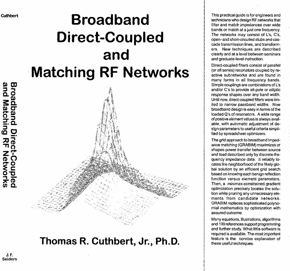


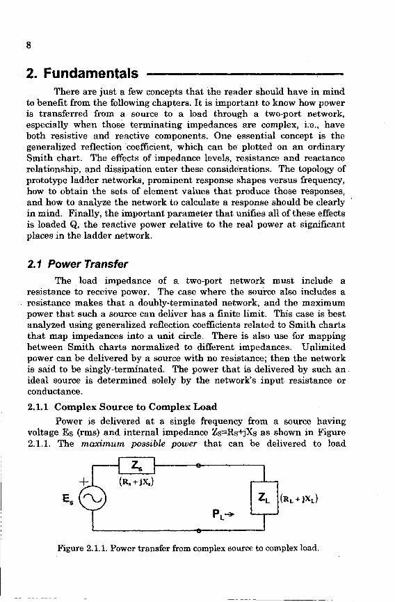
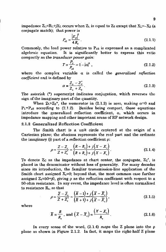
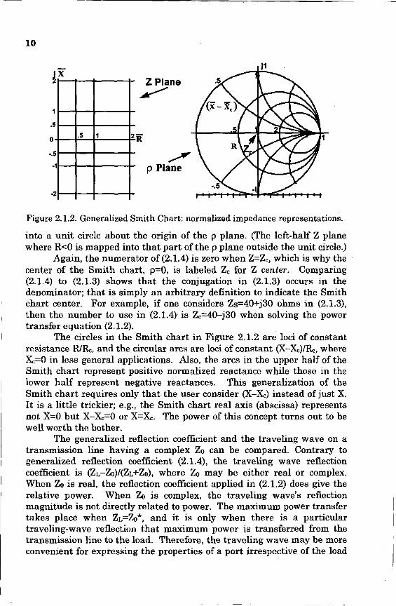
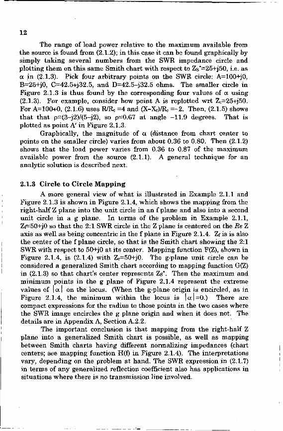
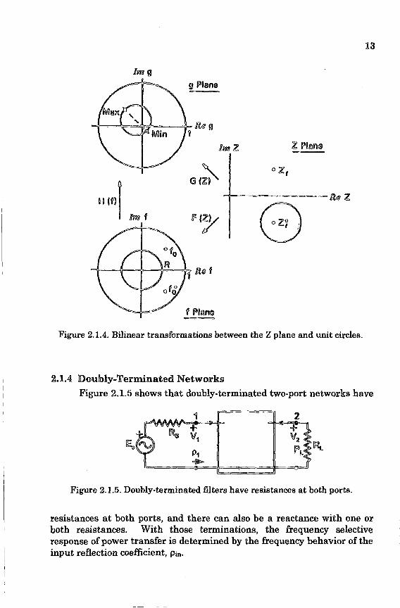

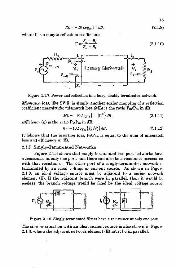
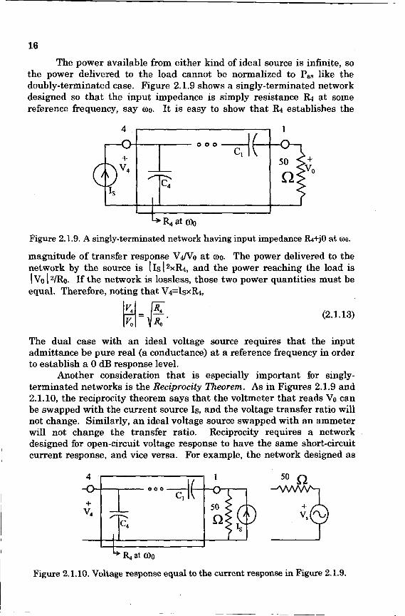
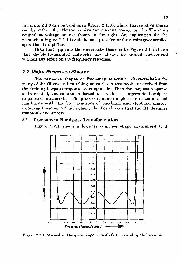
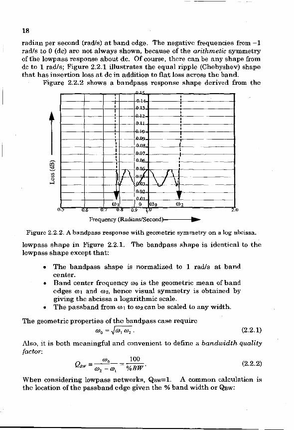

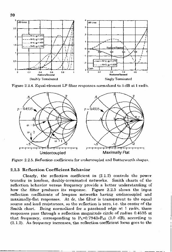


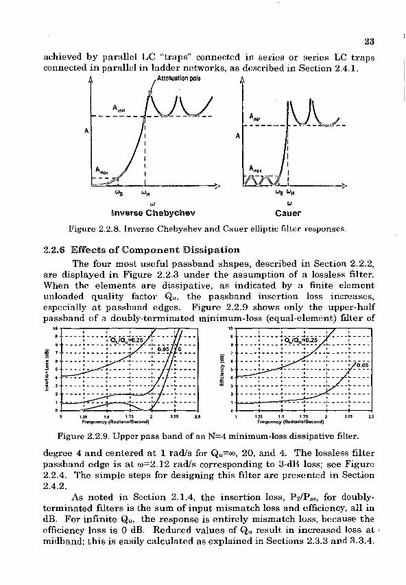
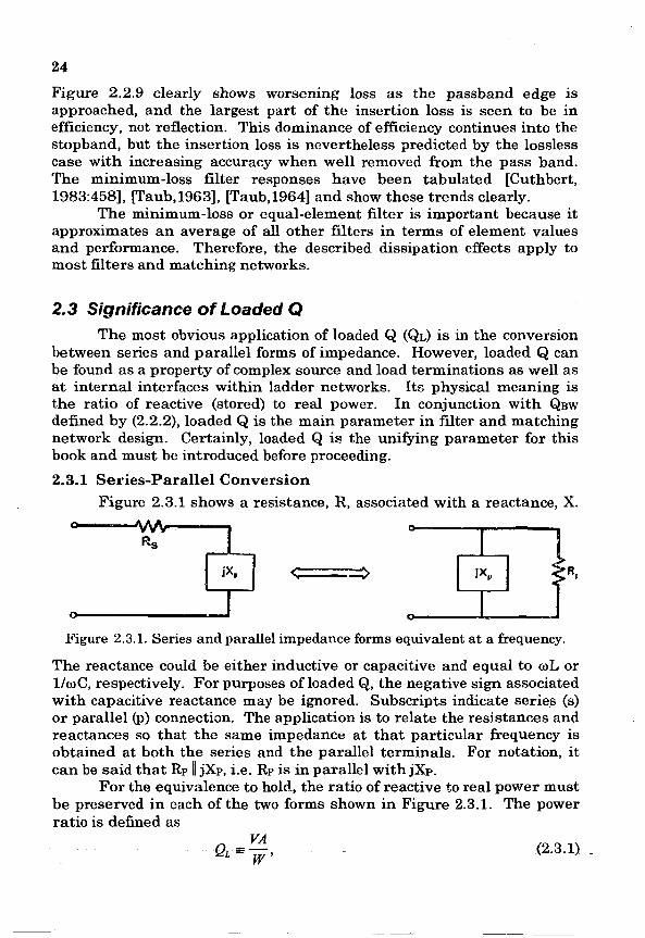
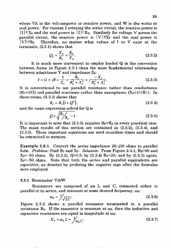
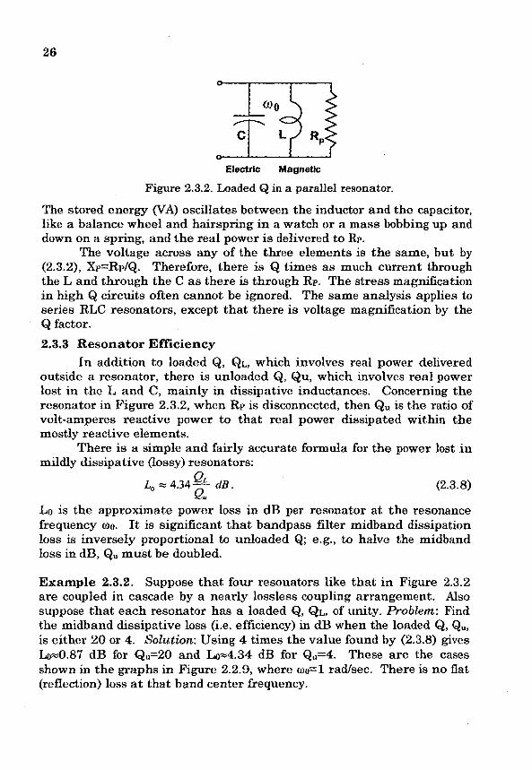
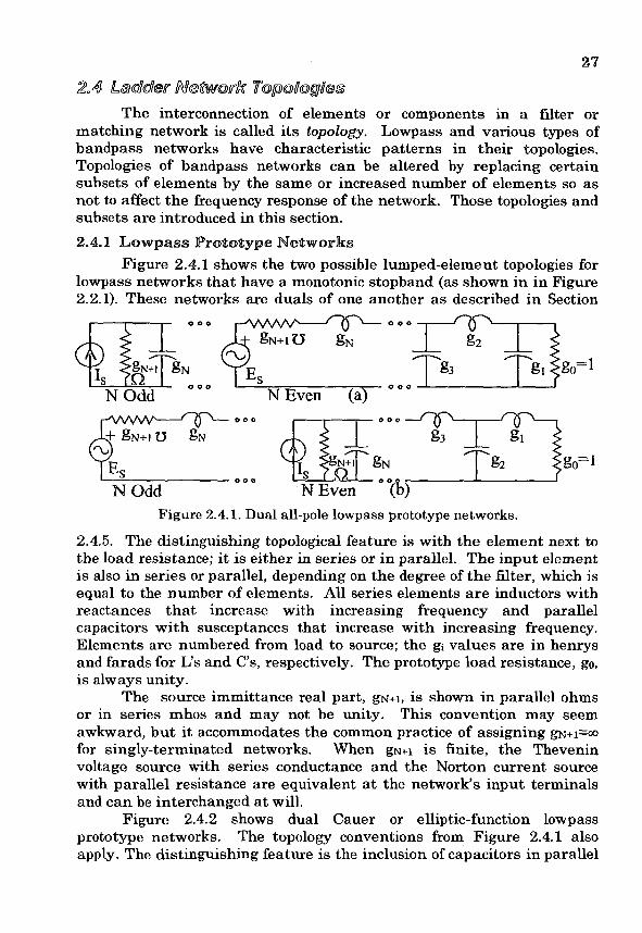
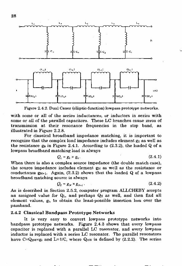
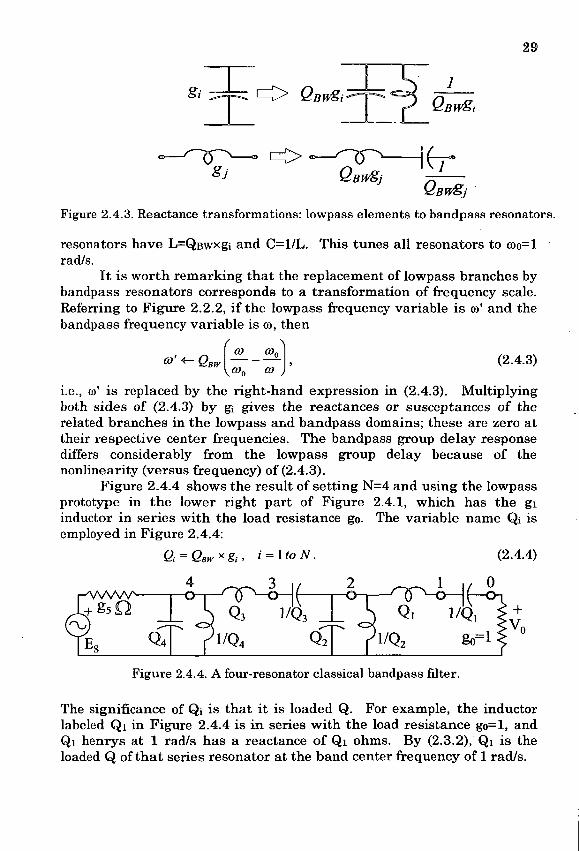
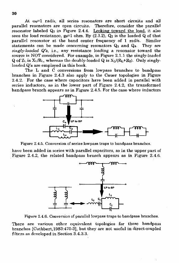
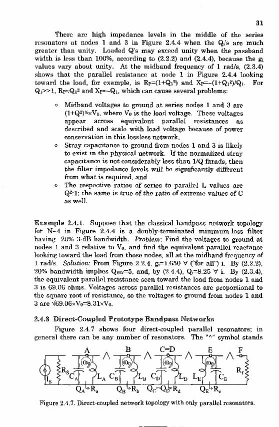
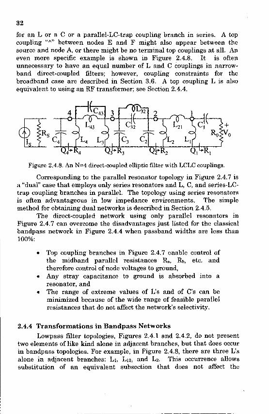
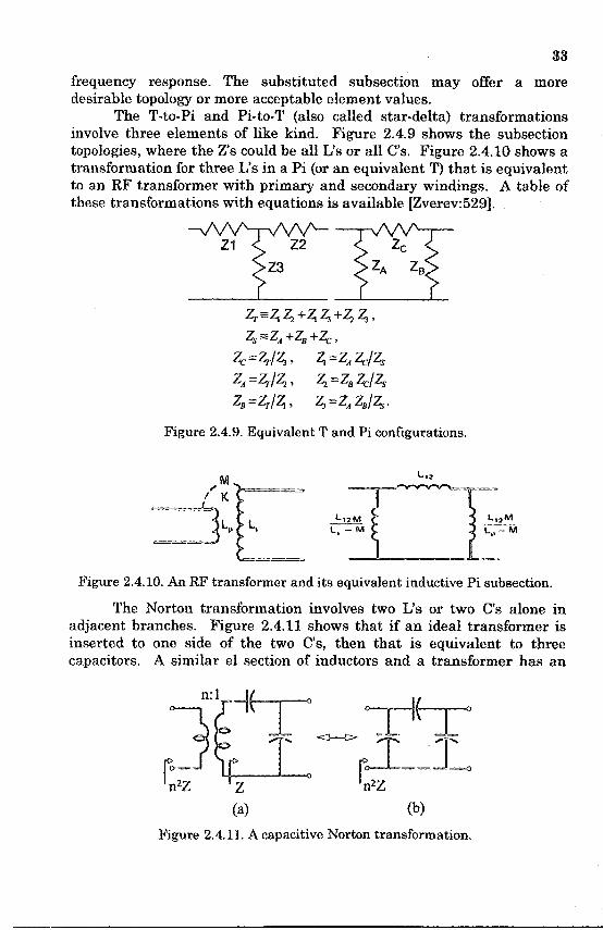
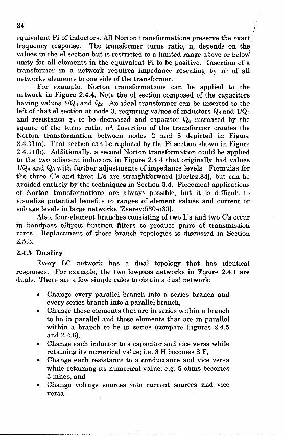
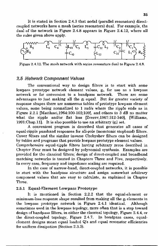
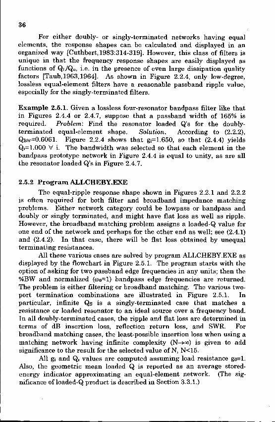
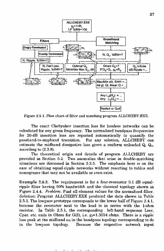
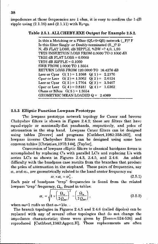
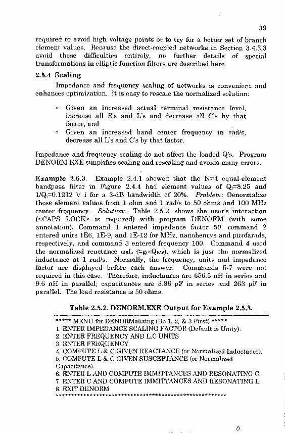
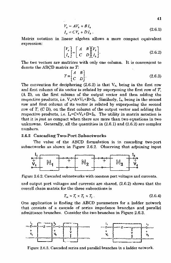
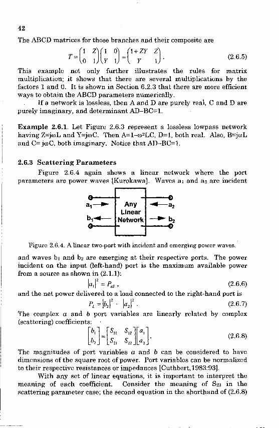

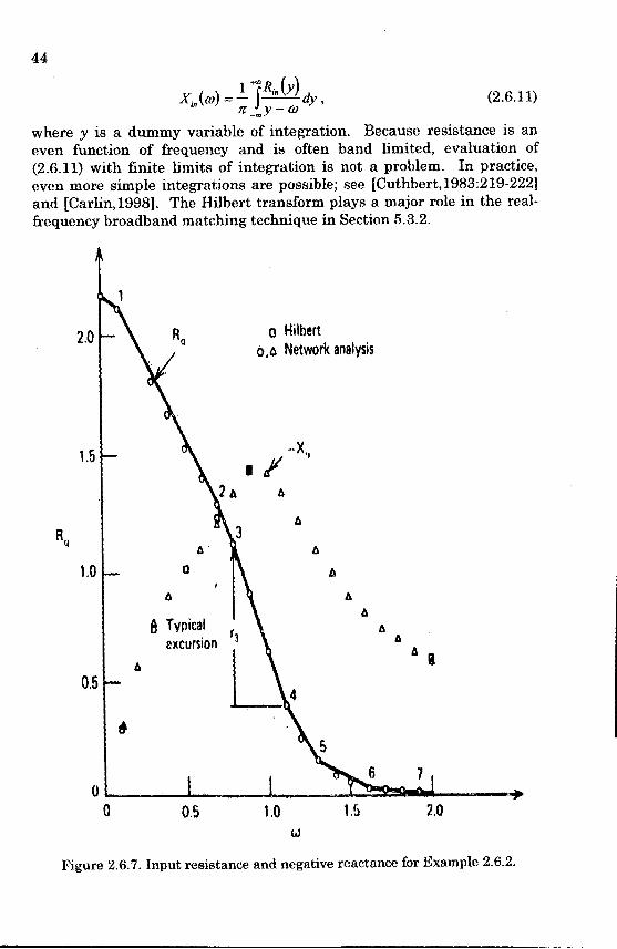
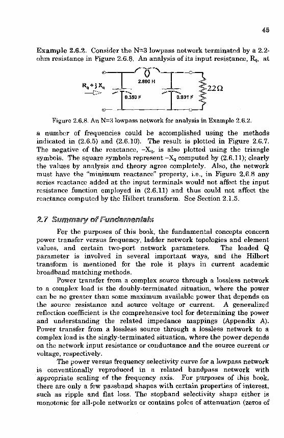

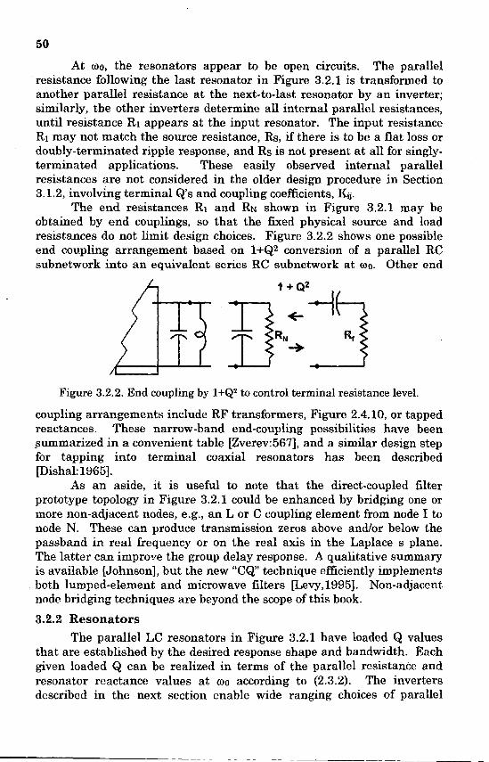
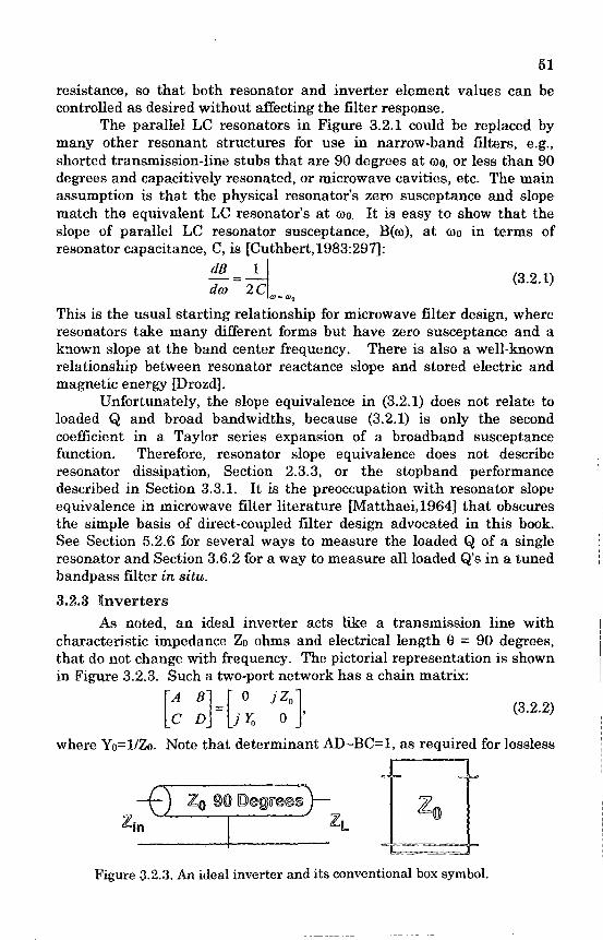
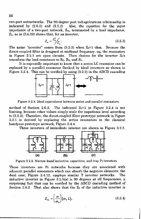
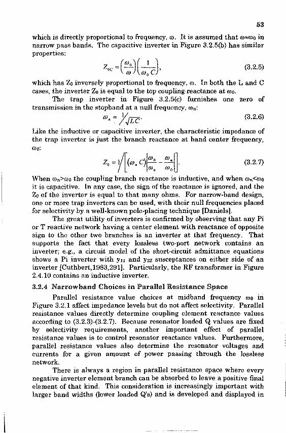
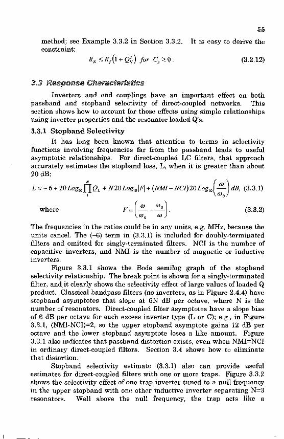
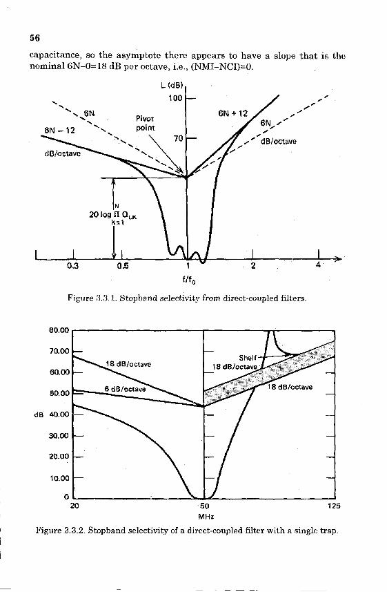
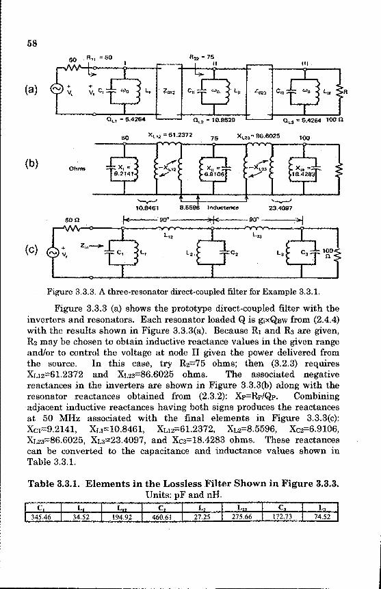
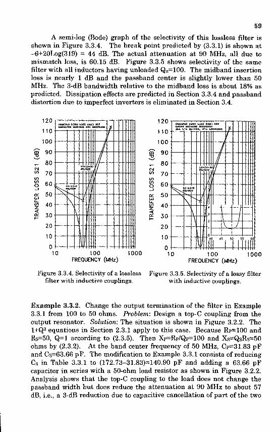

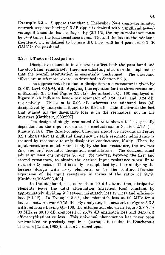
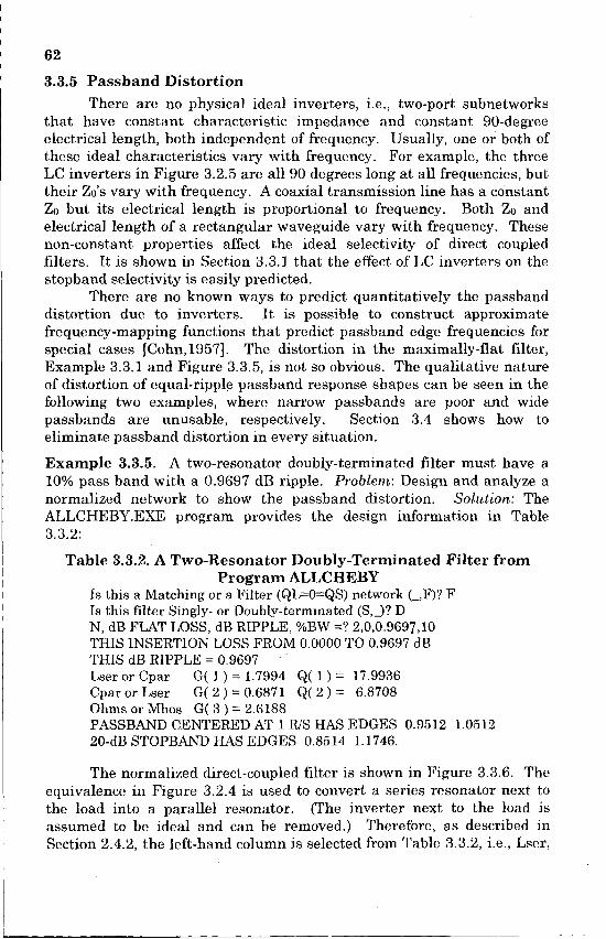
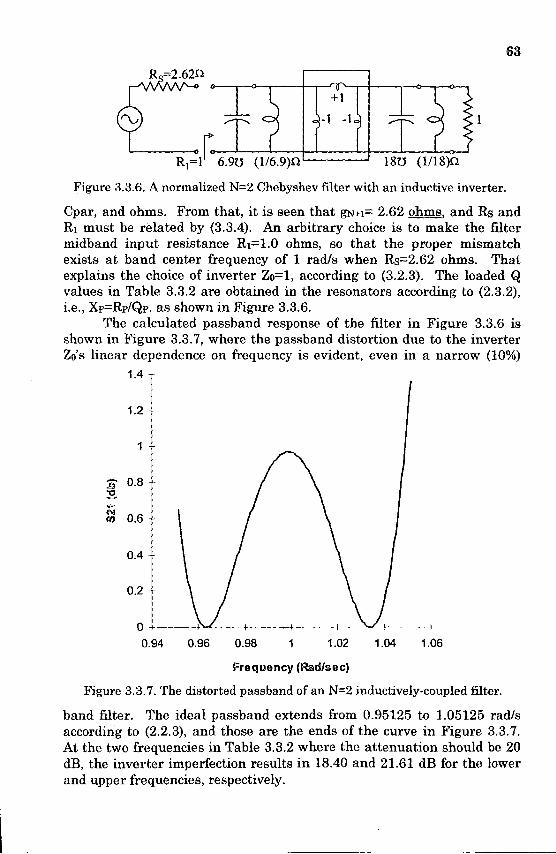
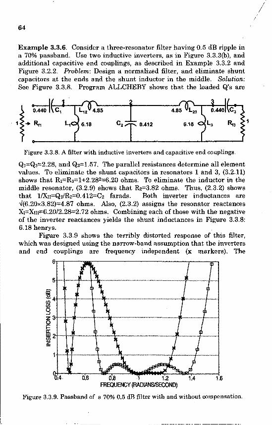
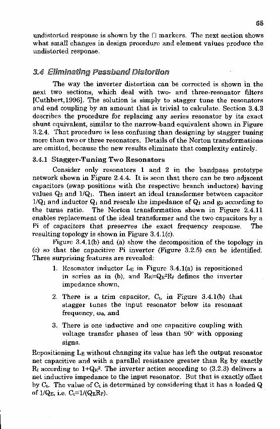
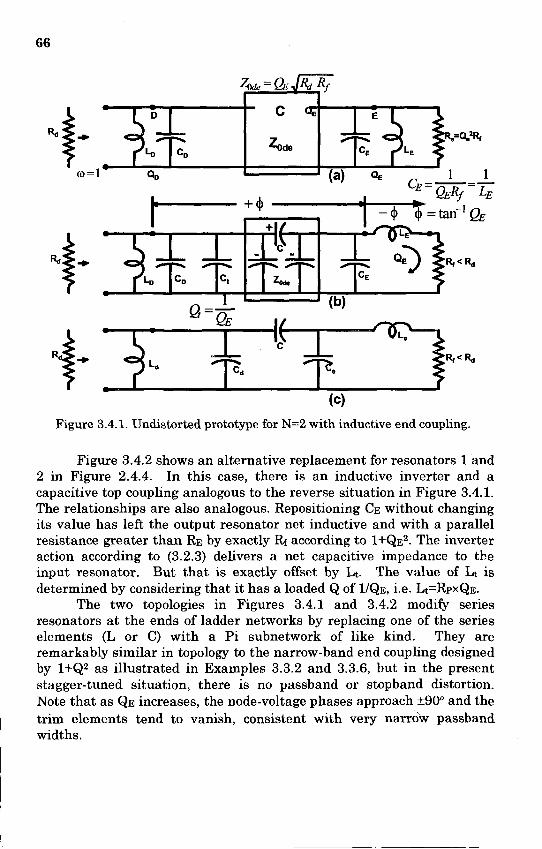
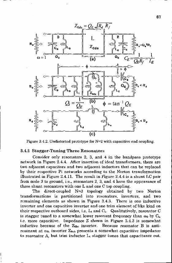
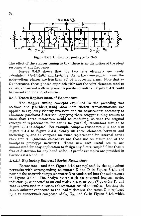
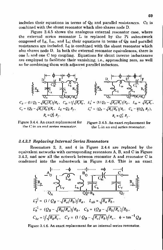
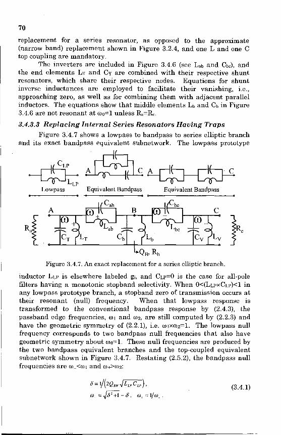
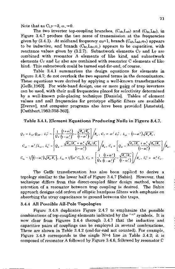
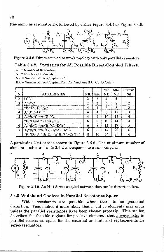
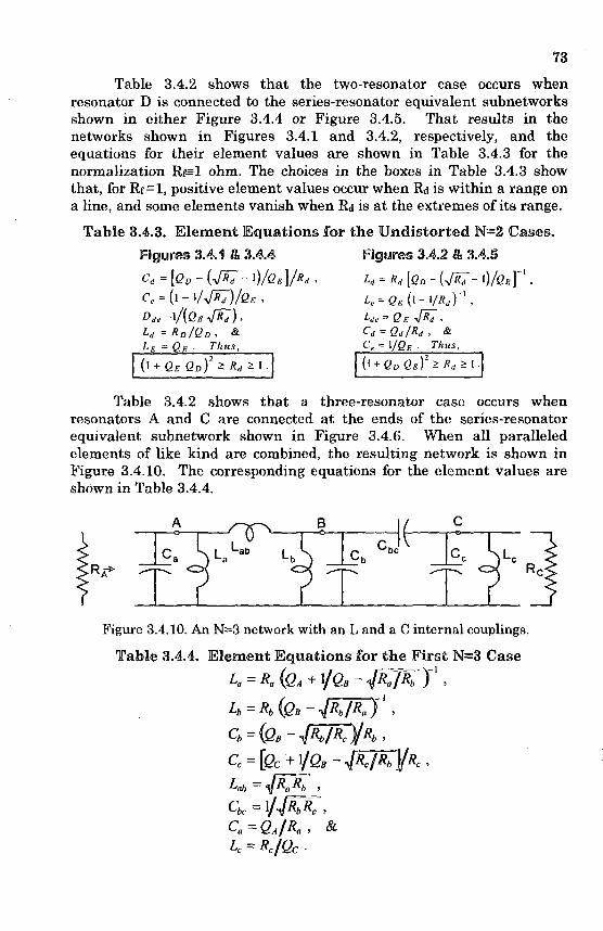
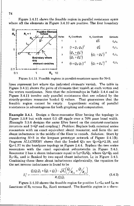
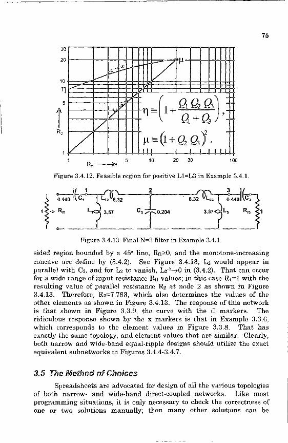
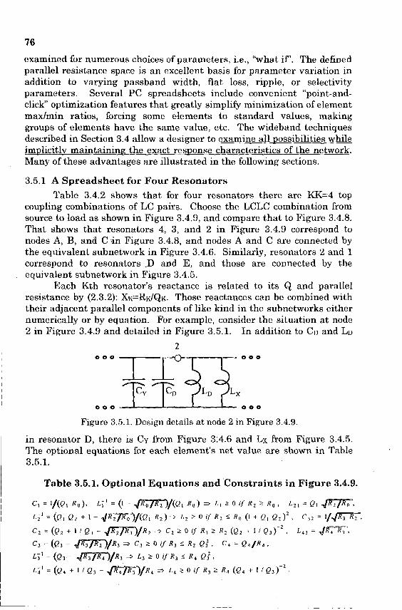
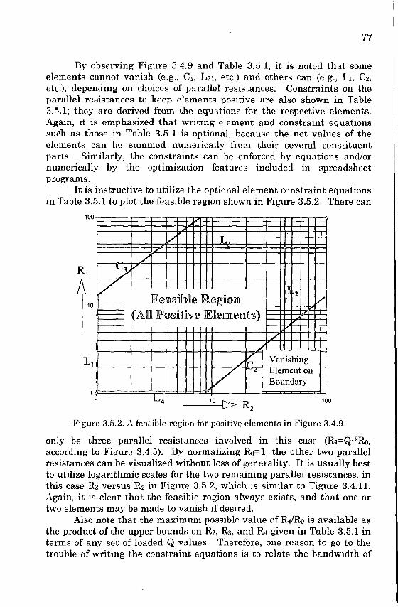
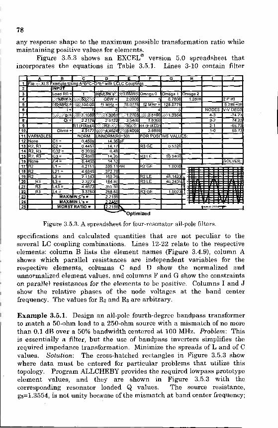
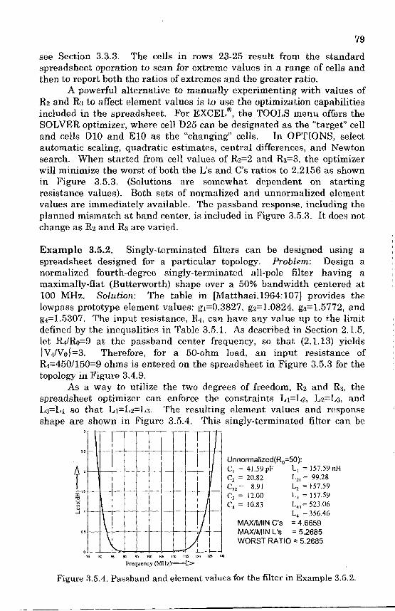
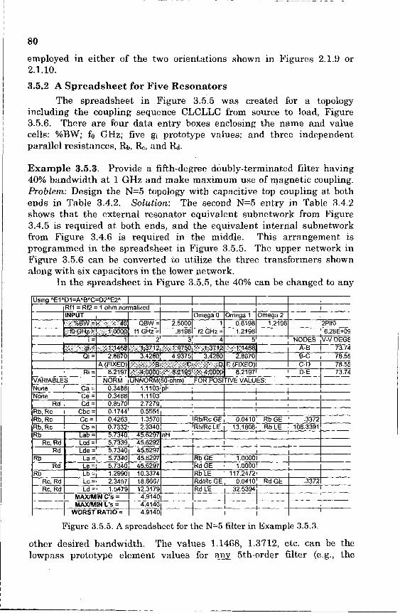
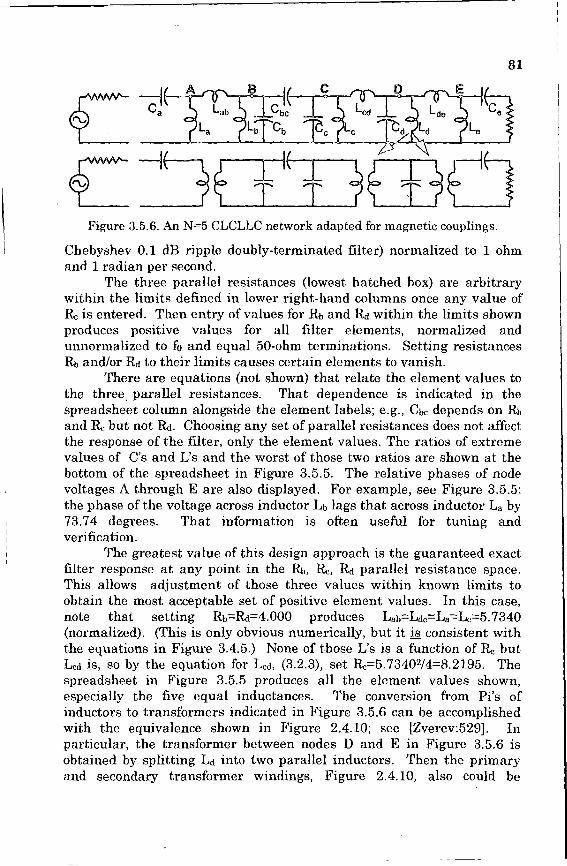
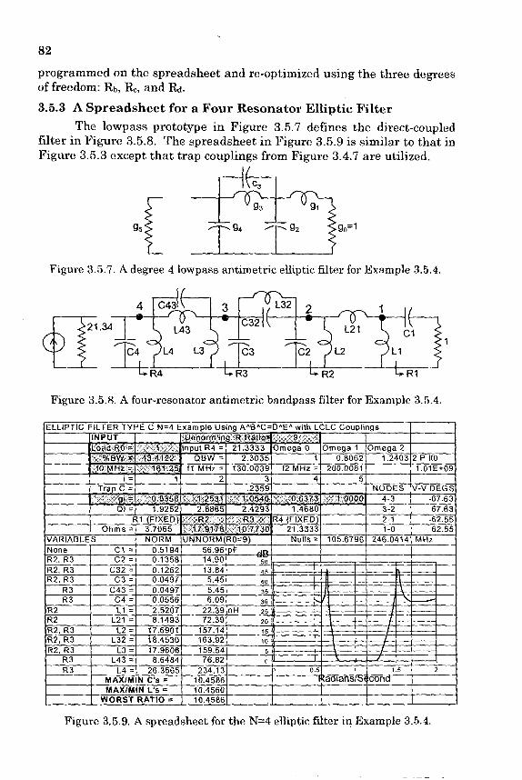
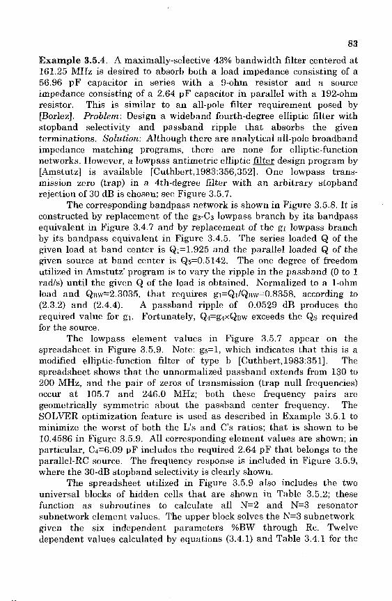
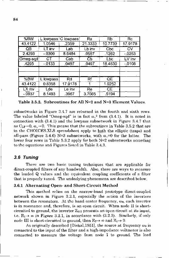
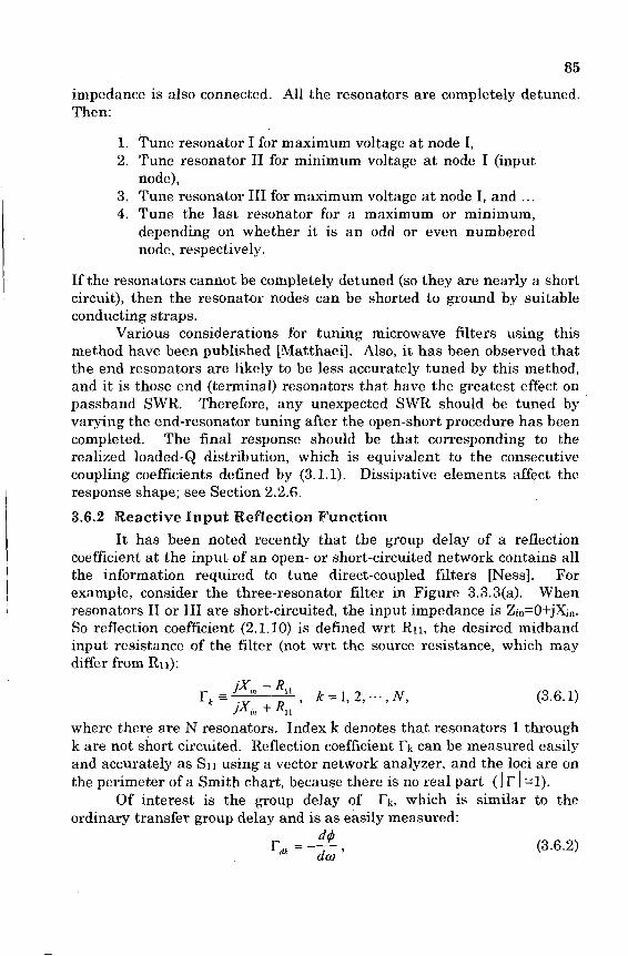
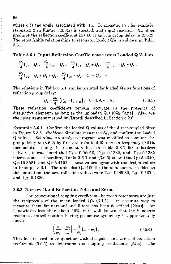
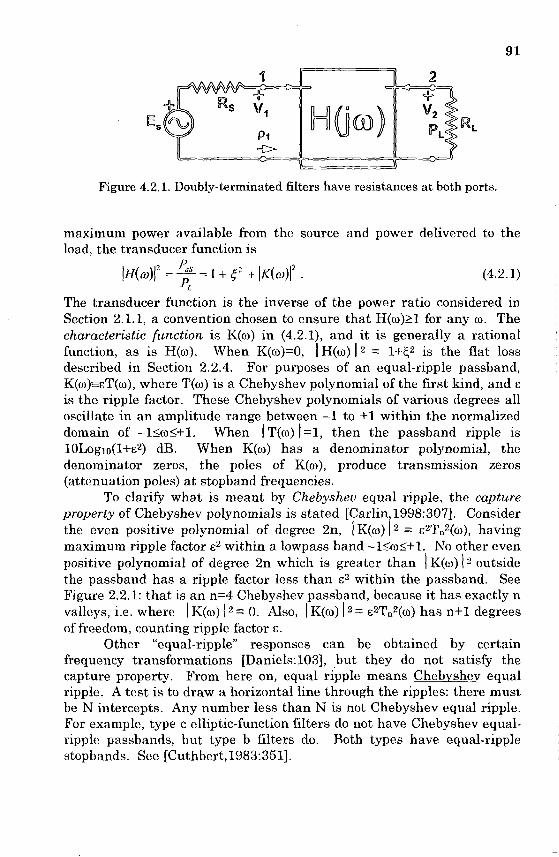
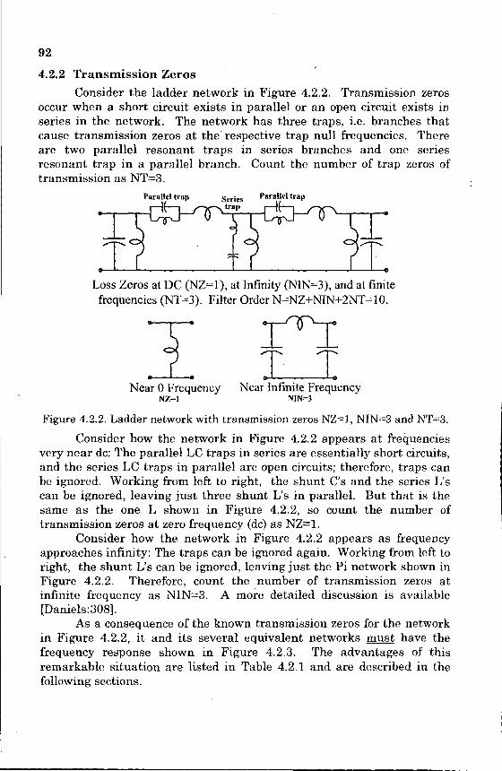
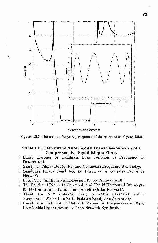
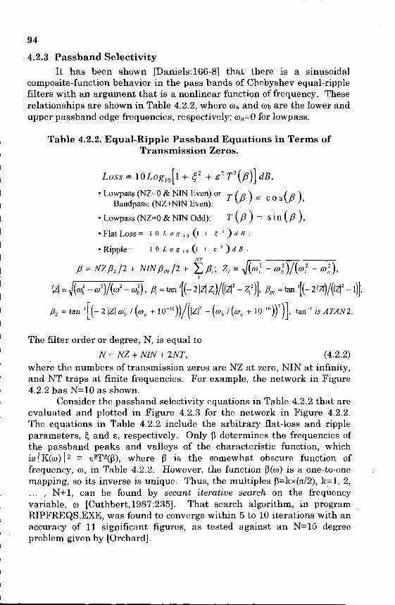

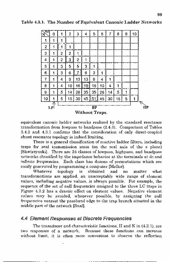
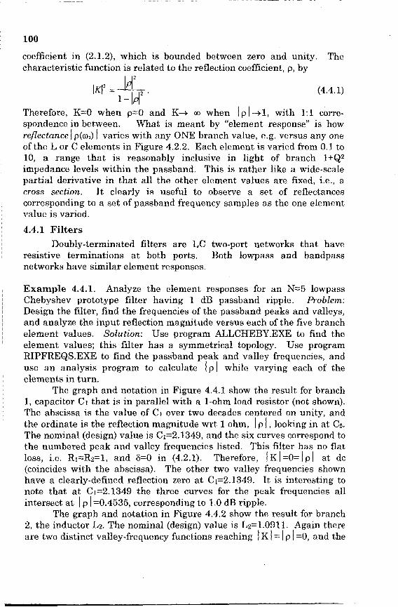
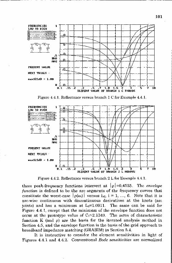
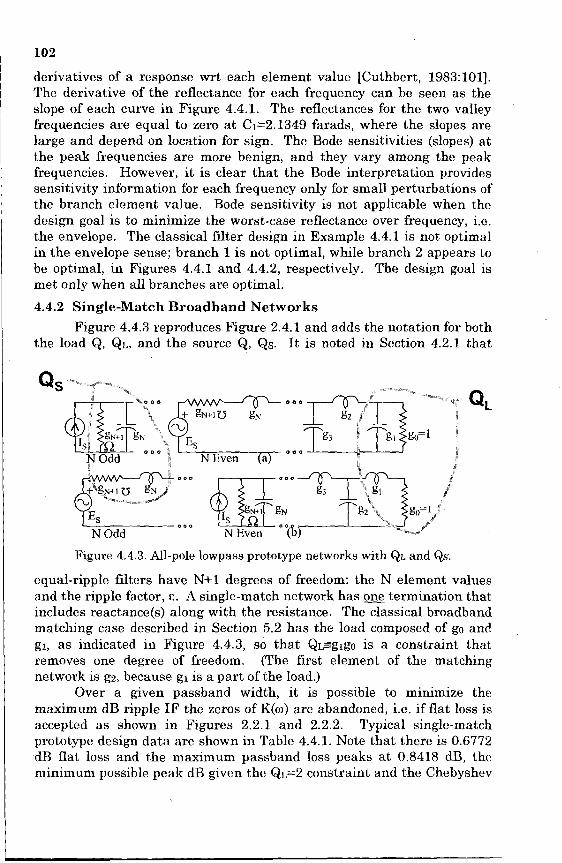
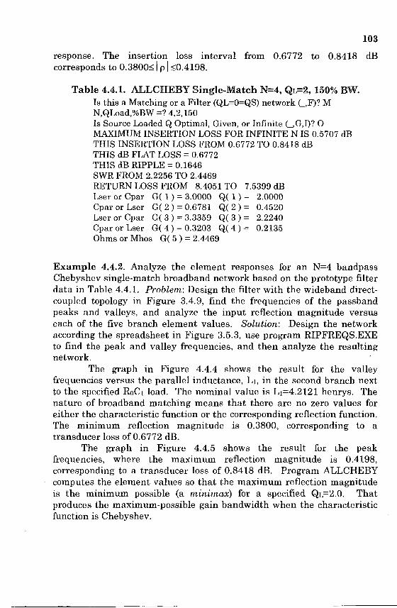
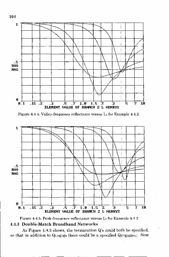
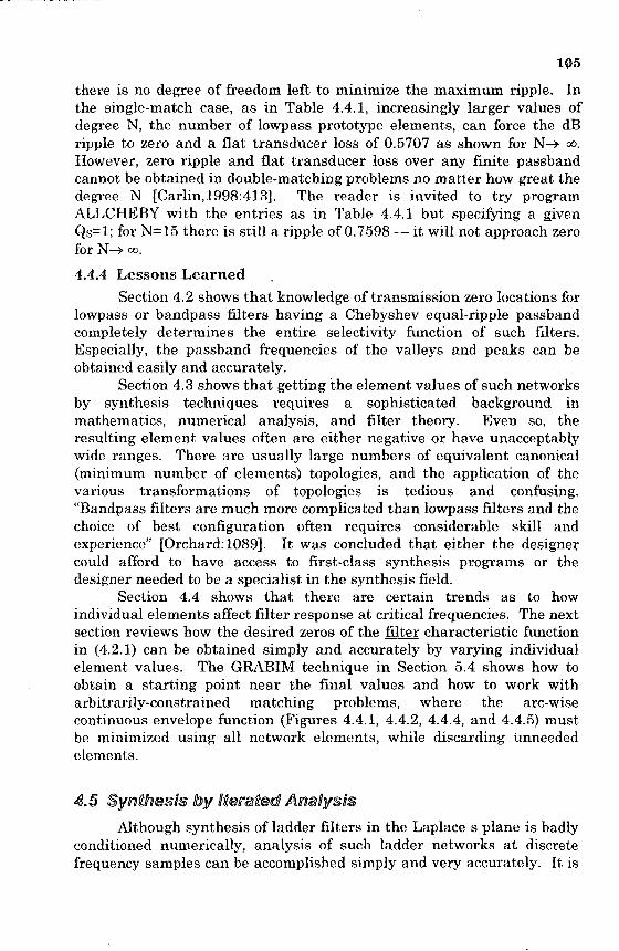

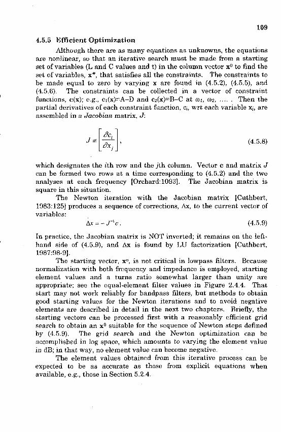
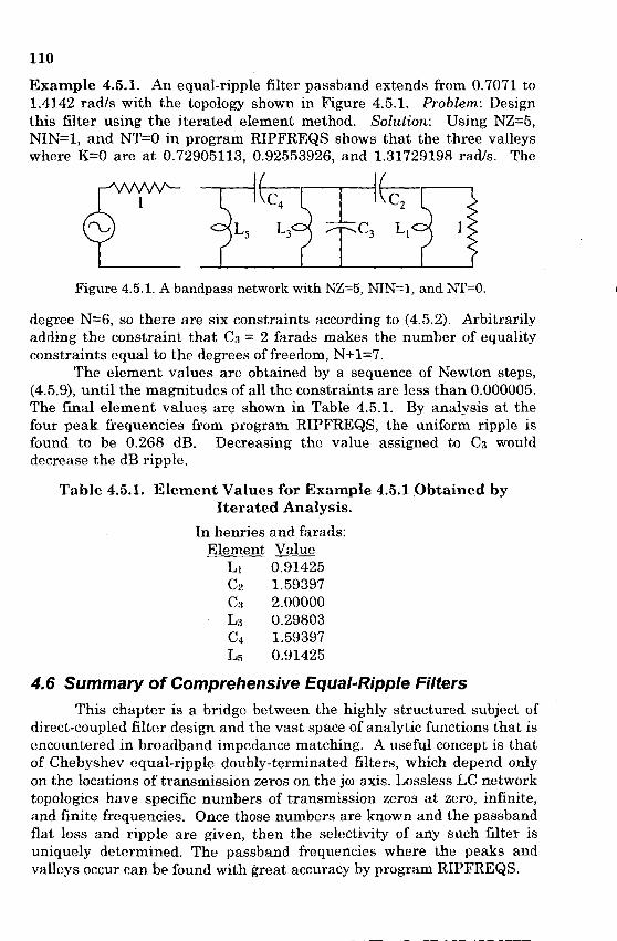
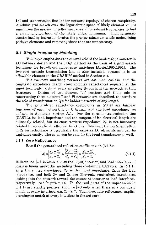
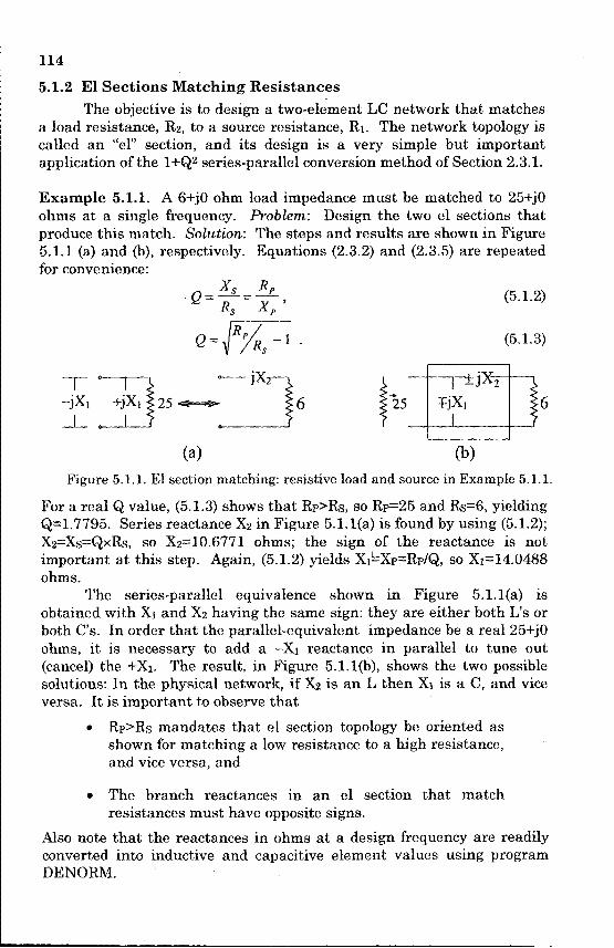
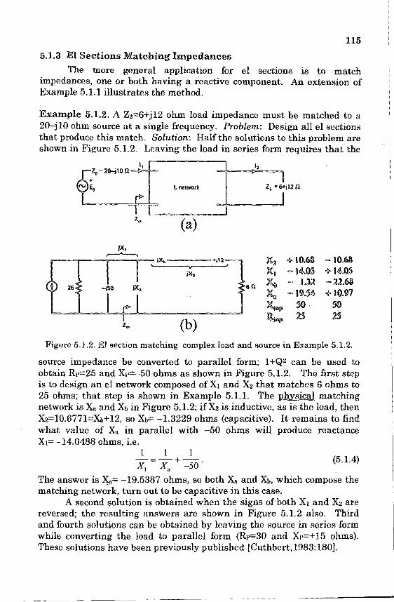
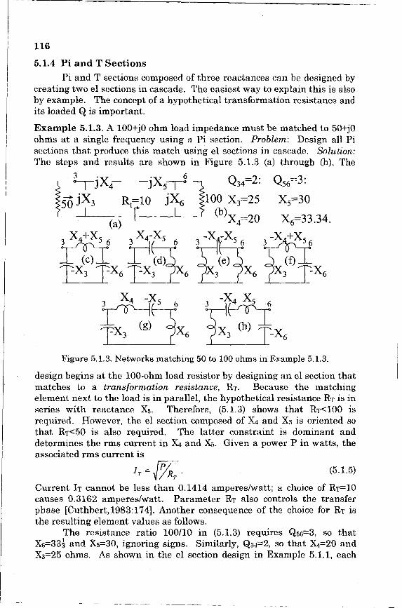
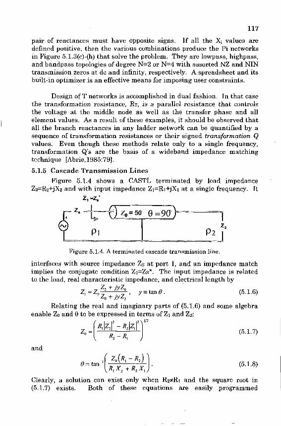
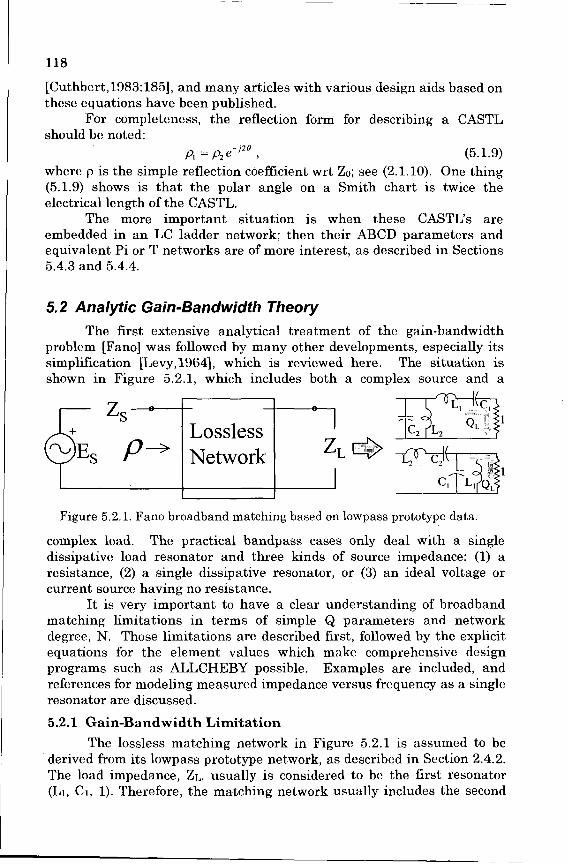
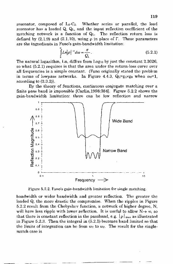
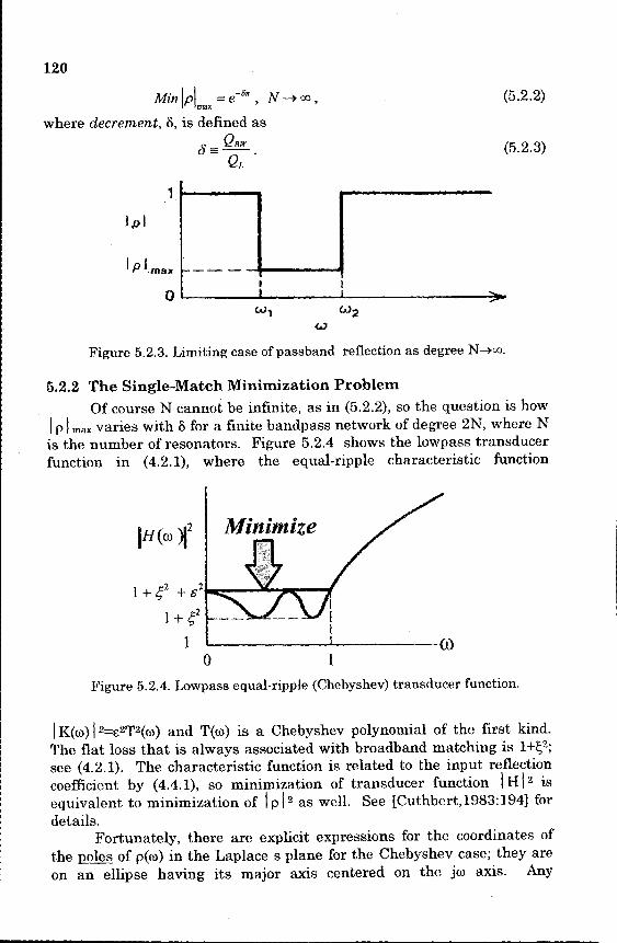
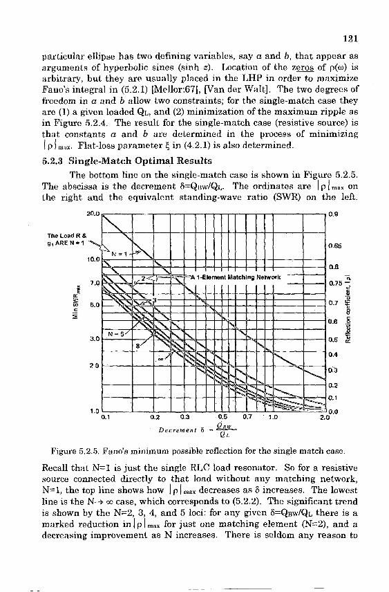
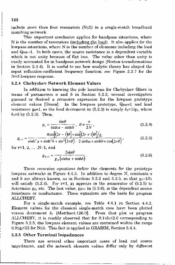
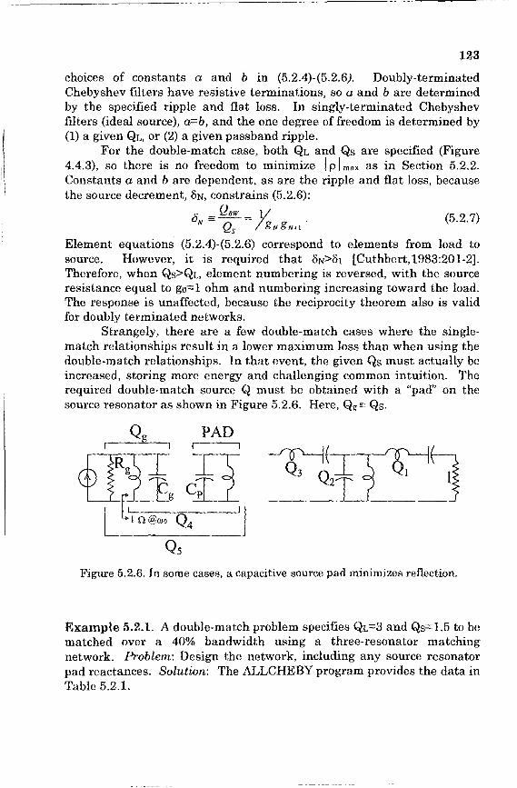

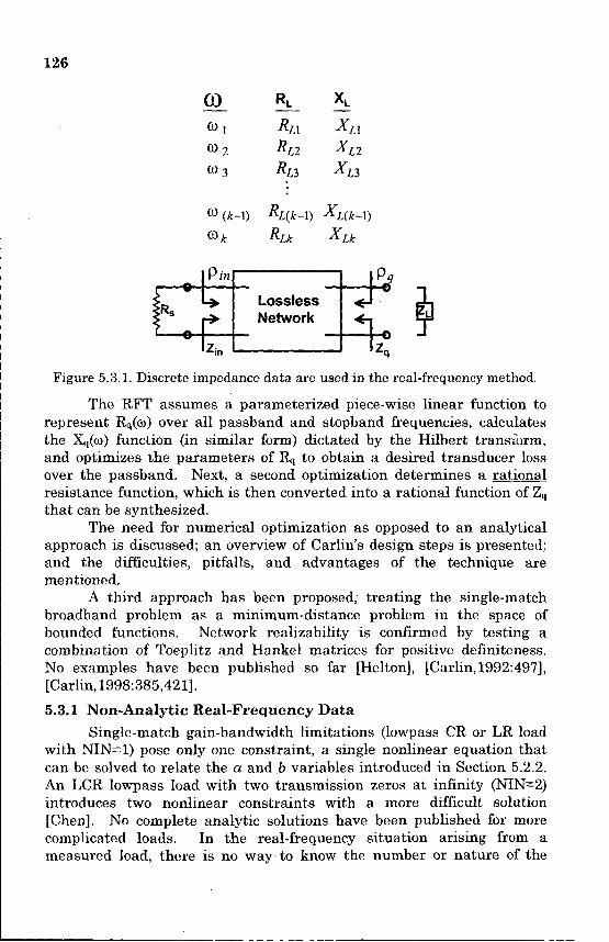
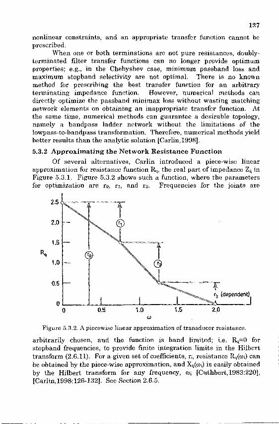

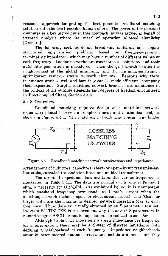
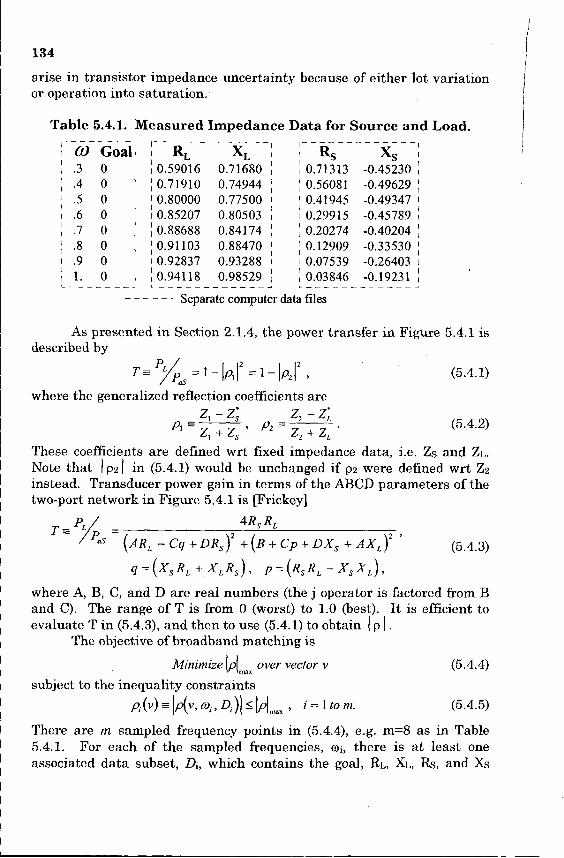
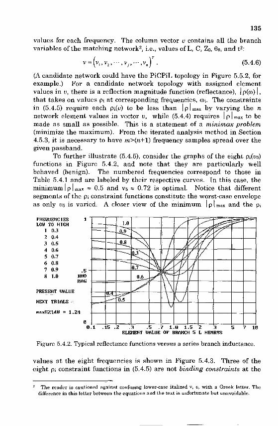
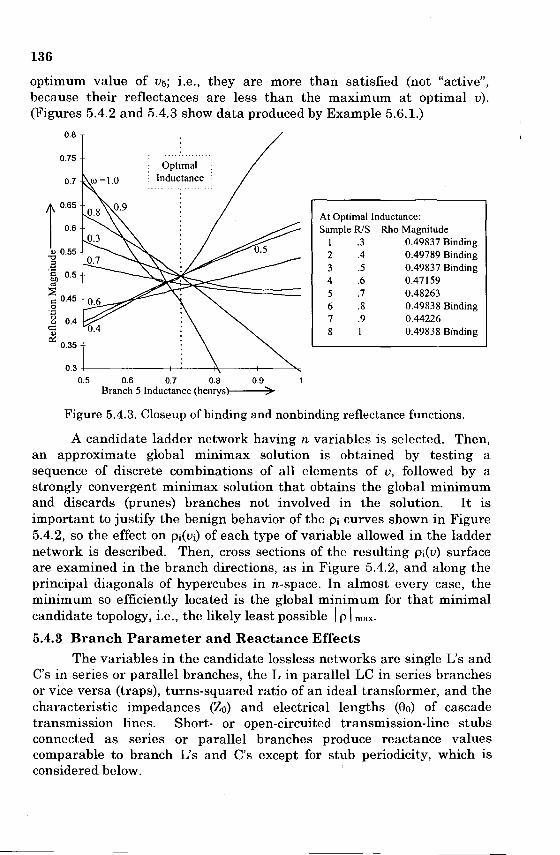
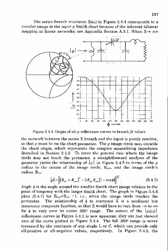
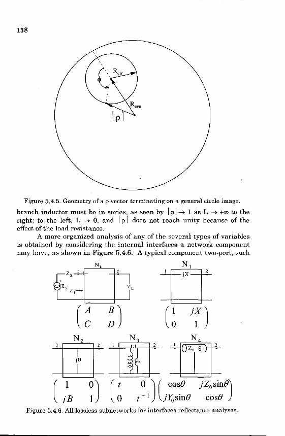
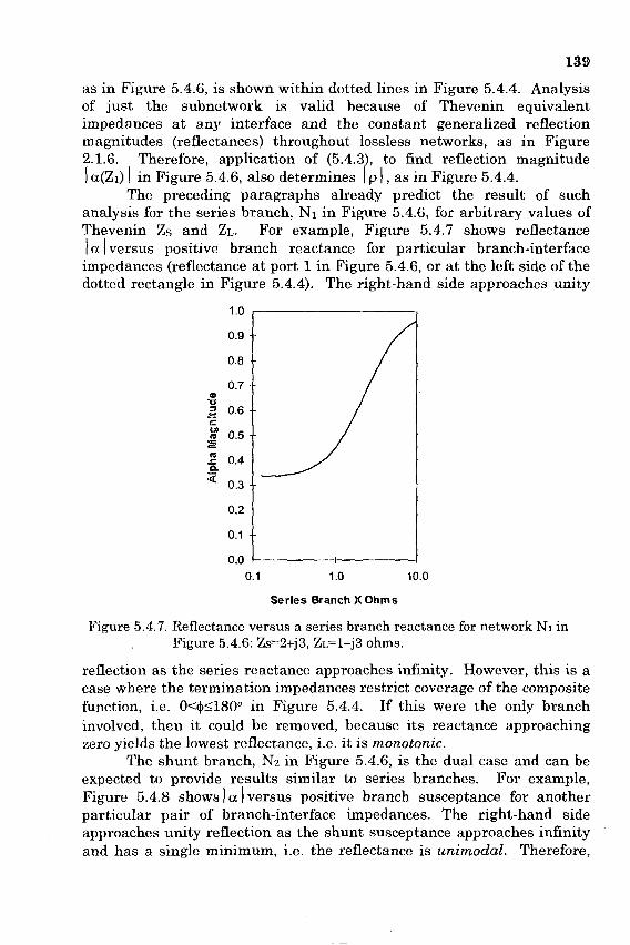
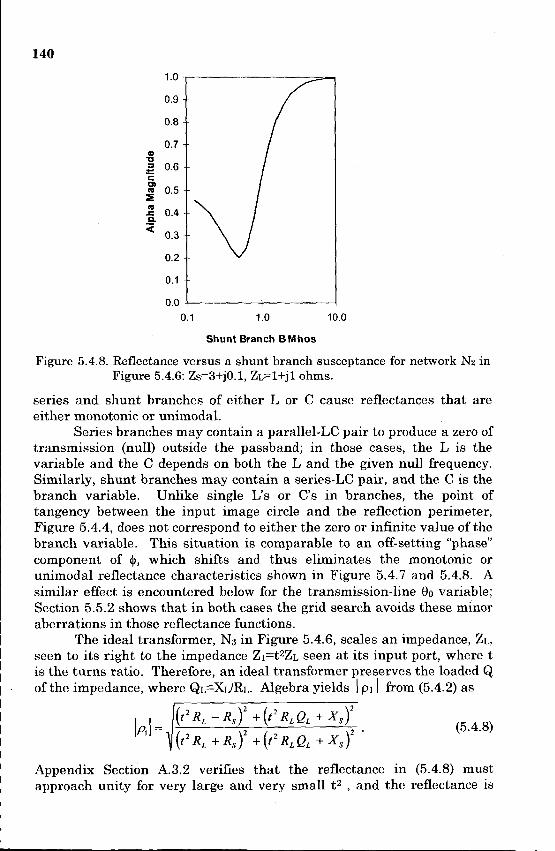
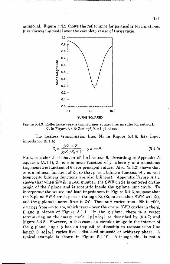
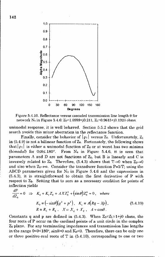

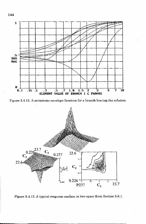
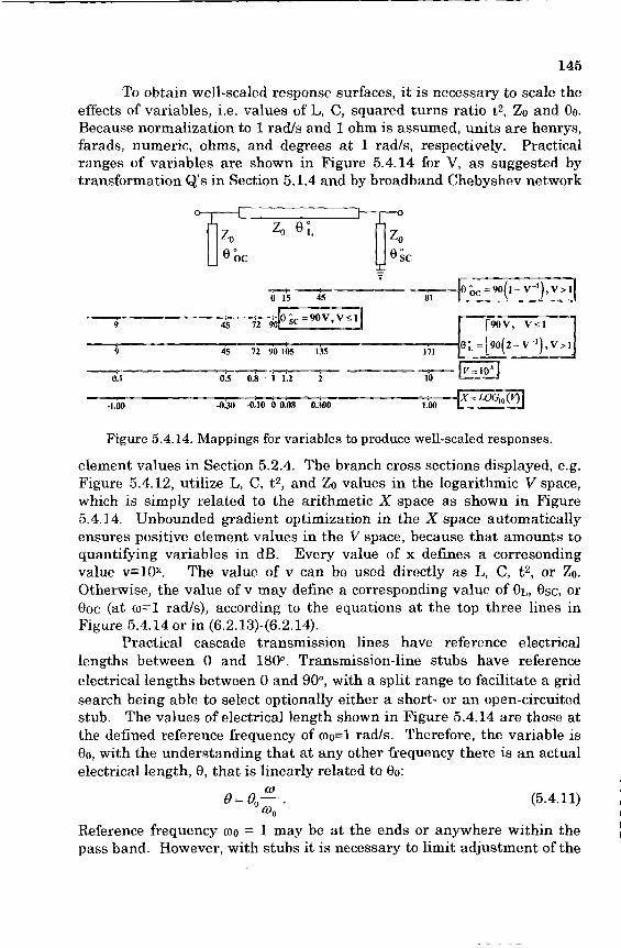
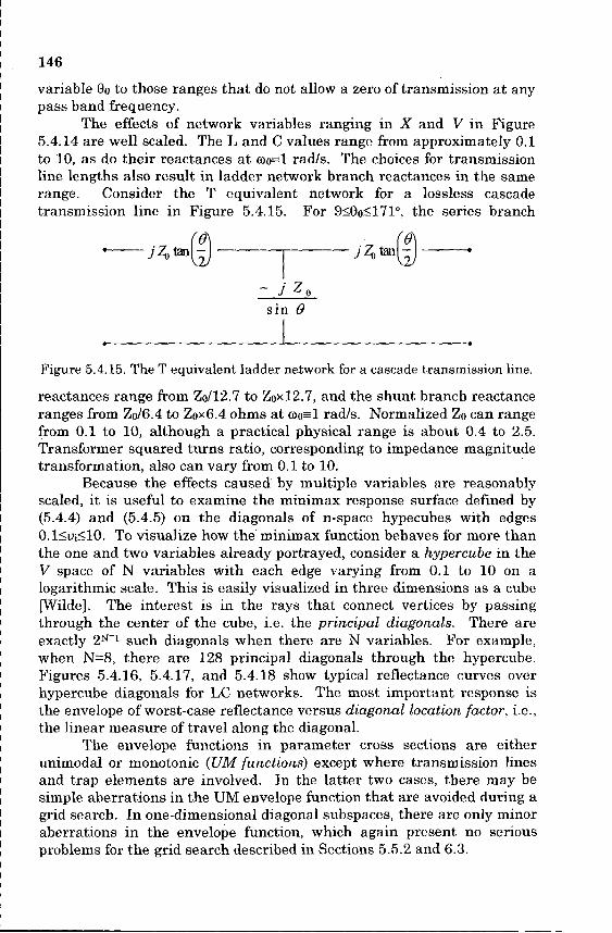
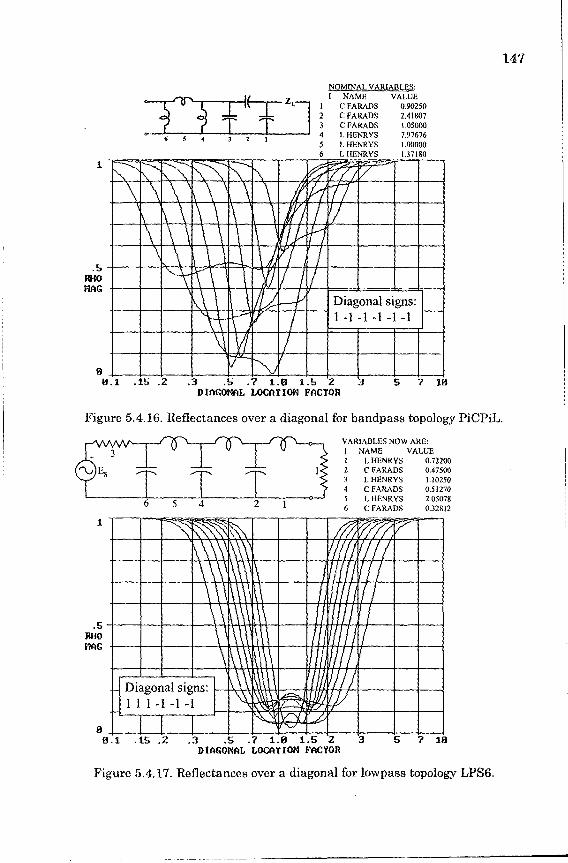
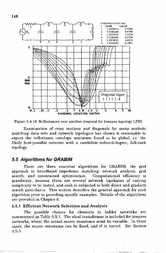
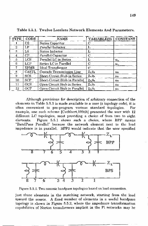
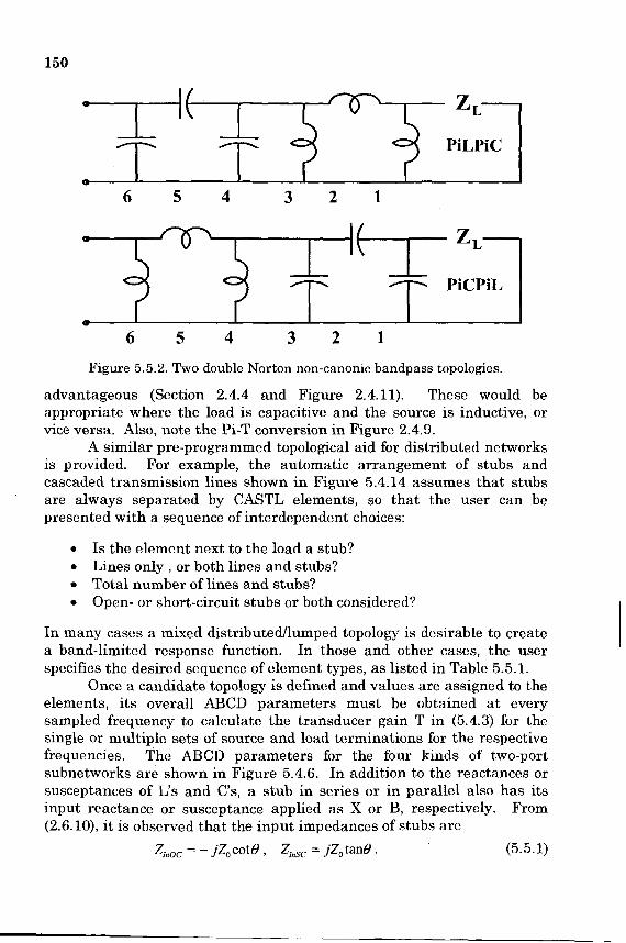
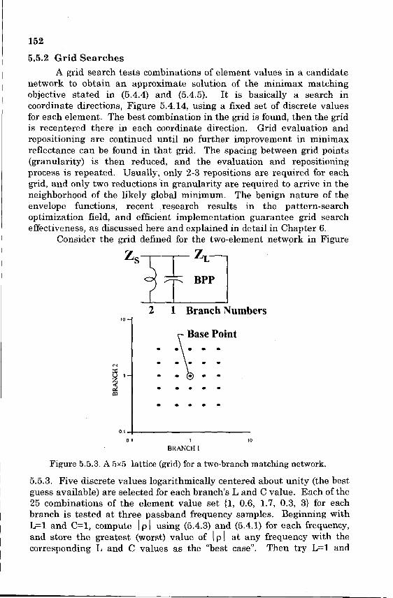
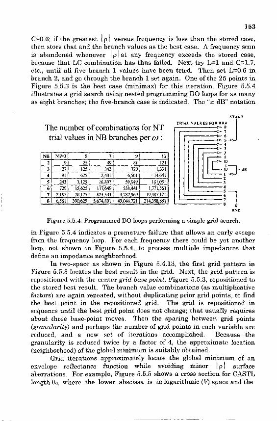
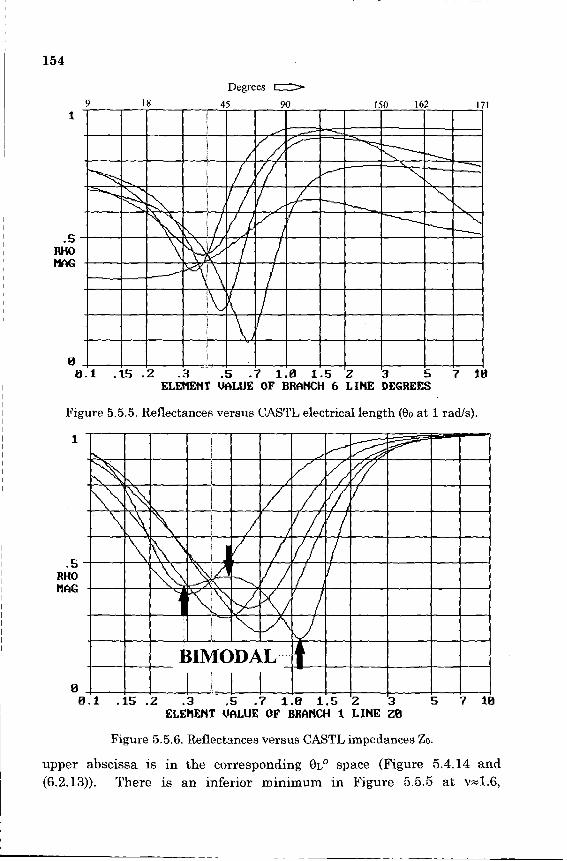
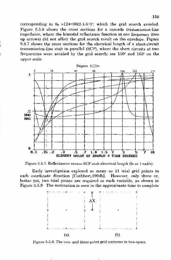
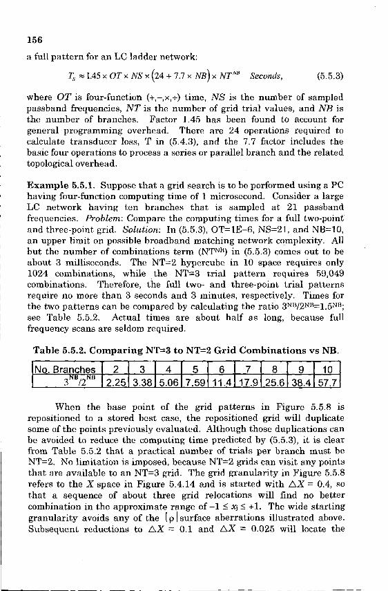
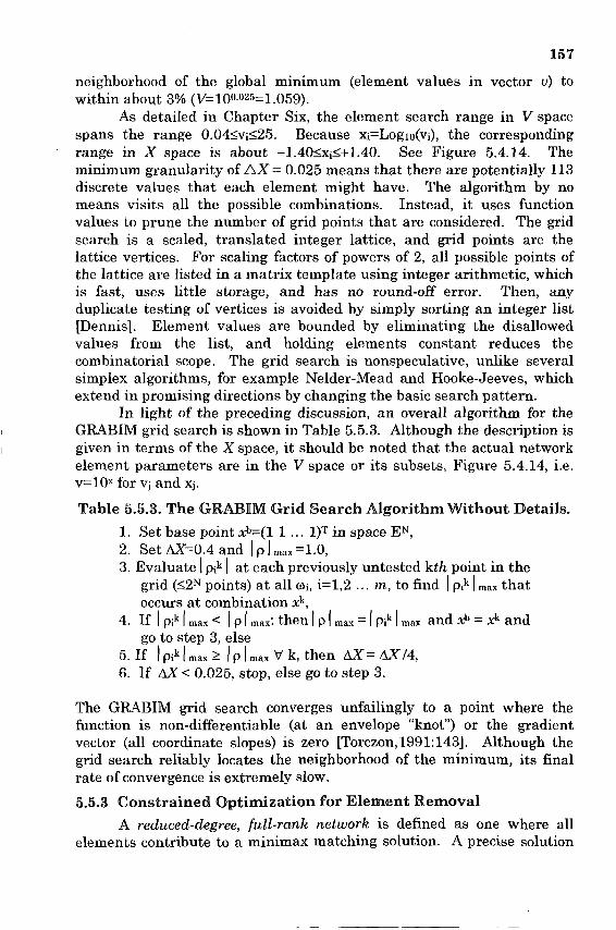
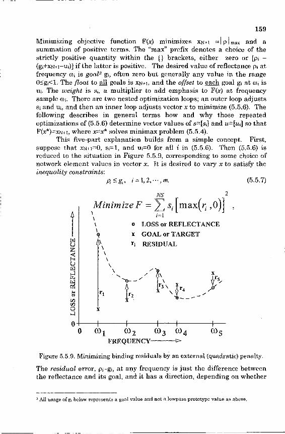
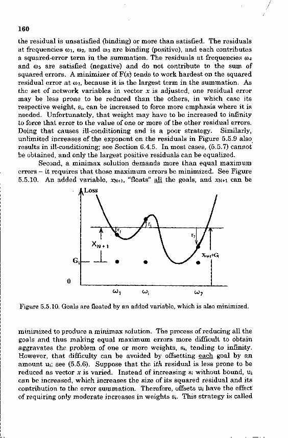
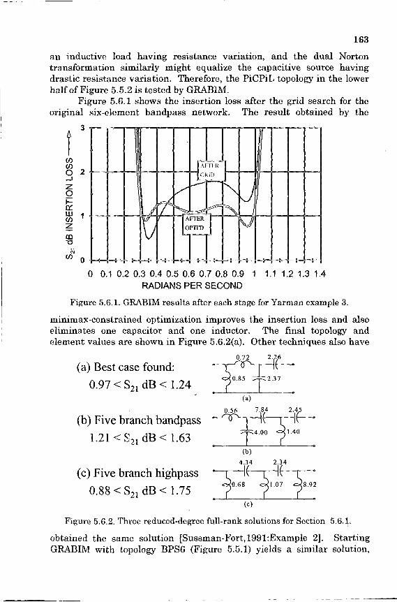
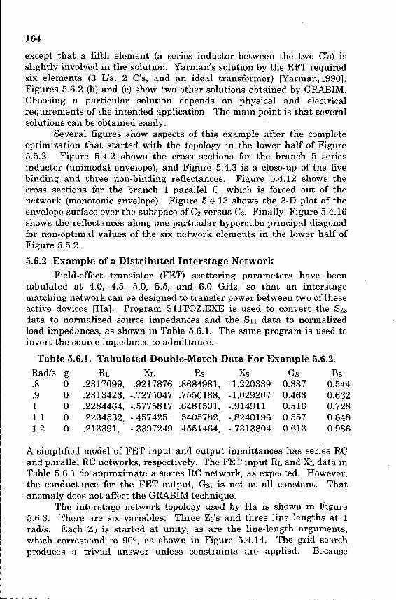
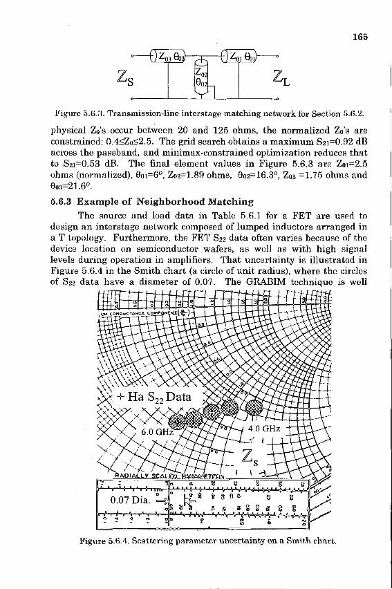
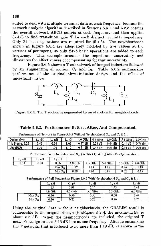
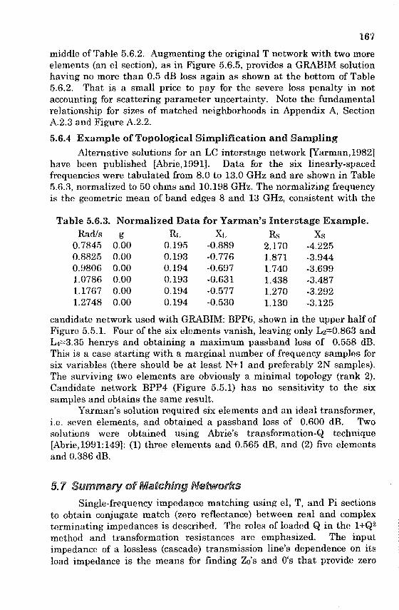

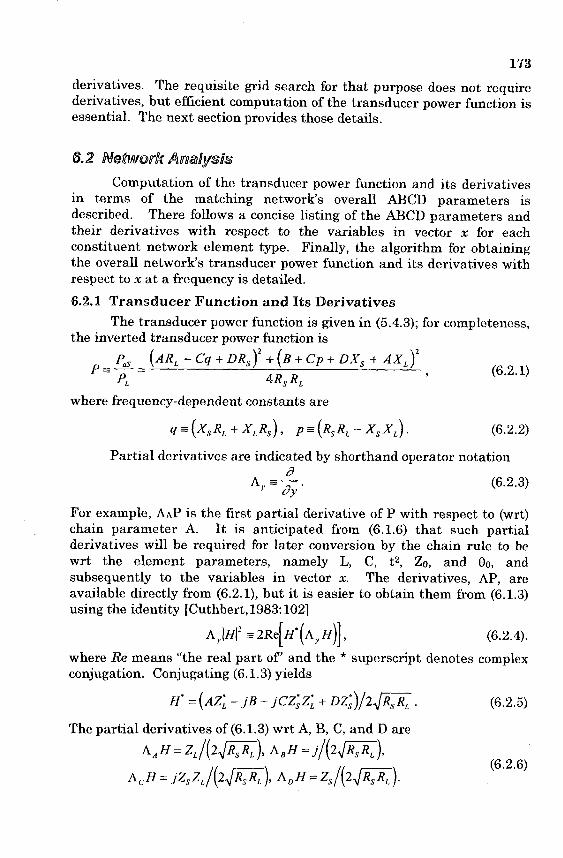
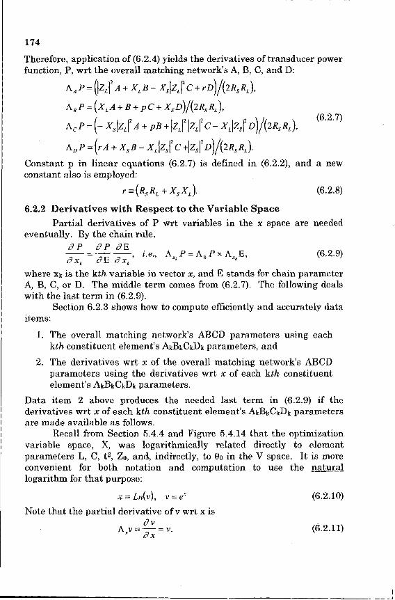
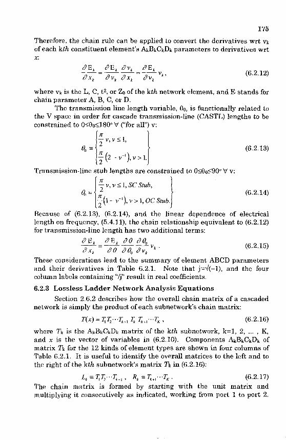
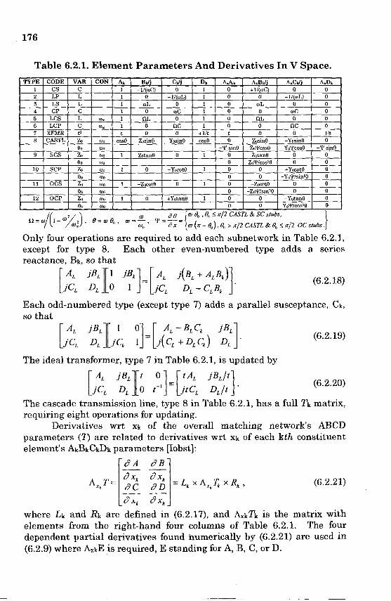
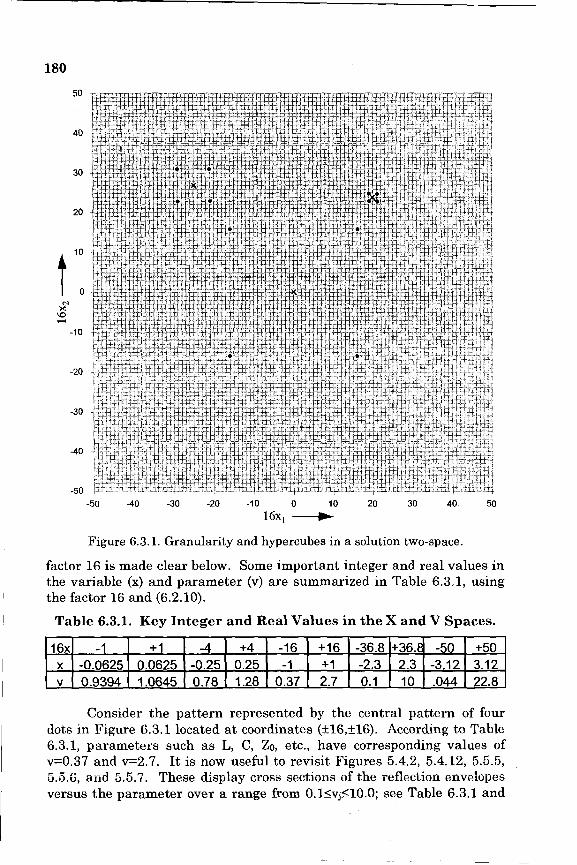
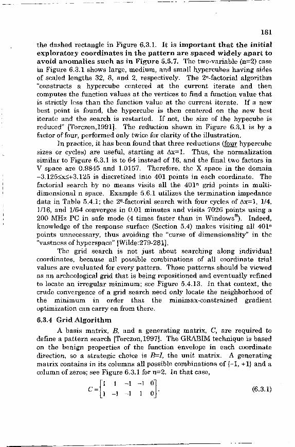


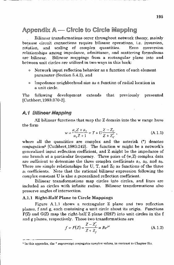

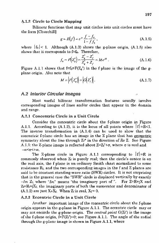

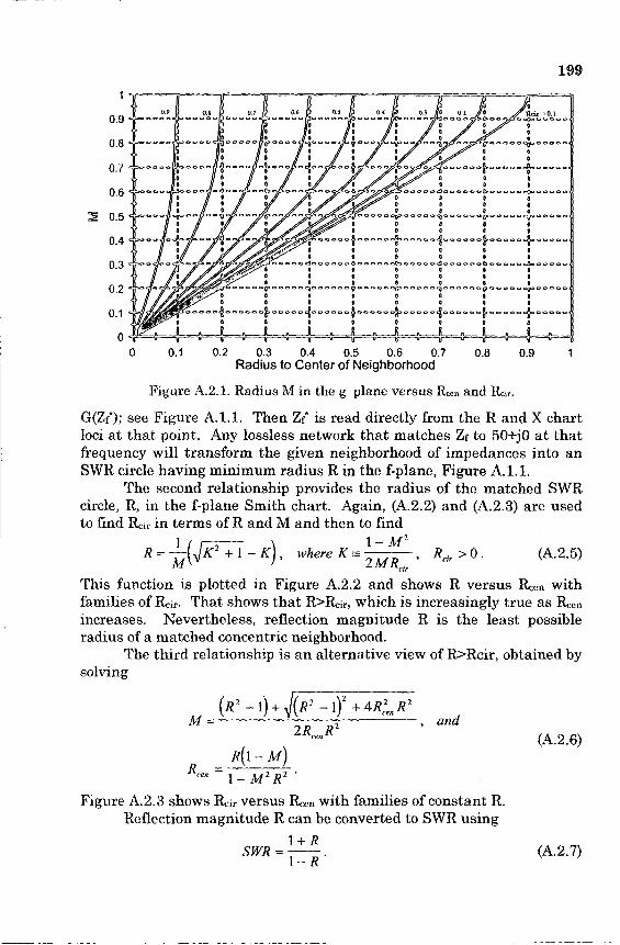
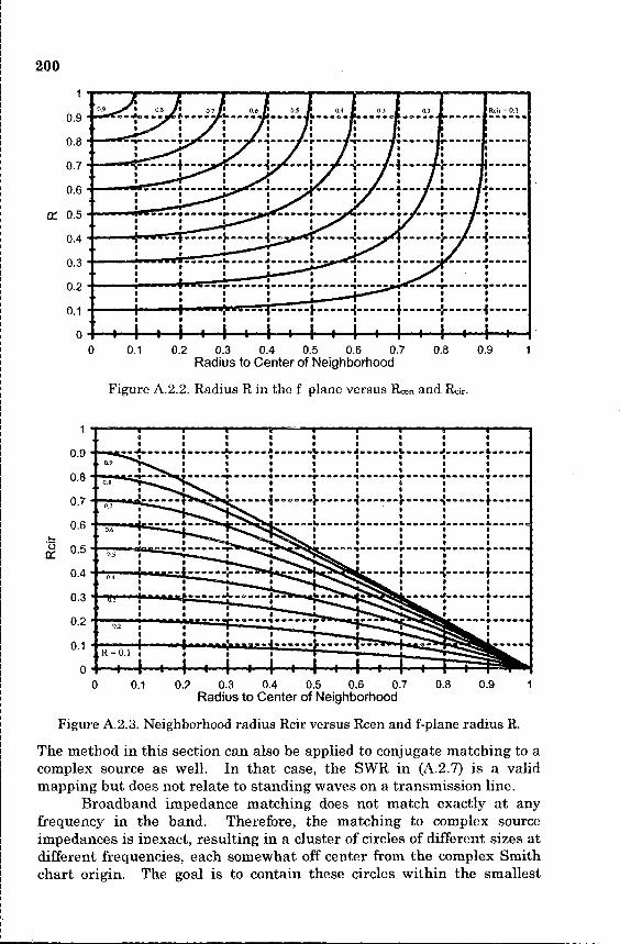
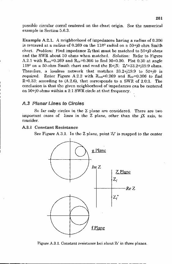
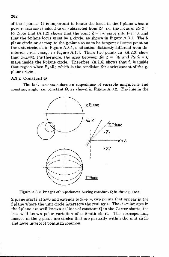
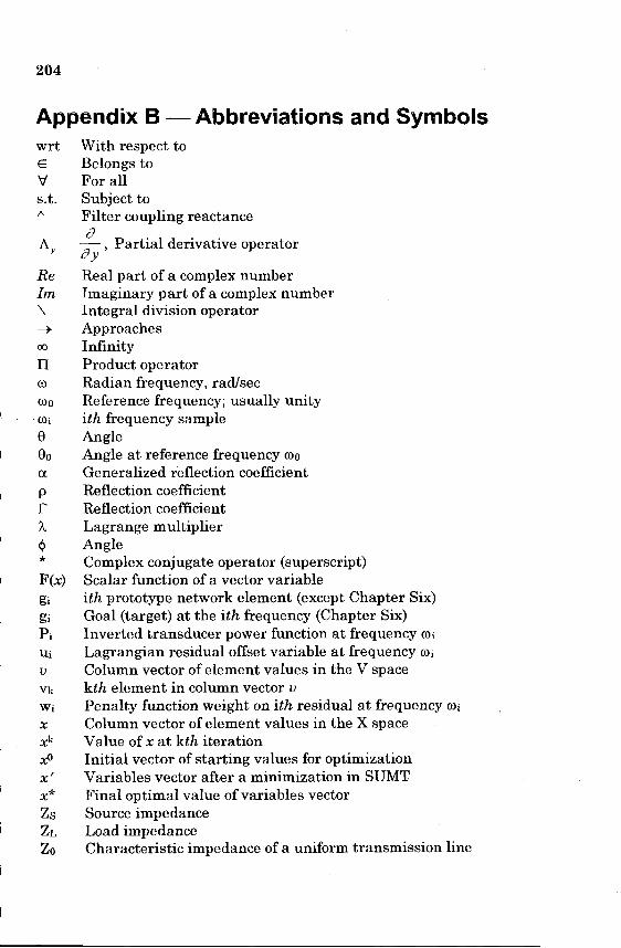


![Digital Chaotic Synchronized Communication System · coupled chaotic circuits and systems has been studied intensely [14] and some interesting applications such as broadband com-munication](https://static.documents.pub/doc/80x56/5e86a95e58f7f502e224fabc/digital-chaotic-synchronized-communication-coupled-chaotic-circuits-and-systems.jpg)


