BSDEs, martingale problems, pseudo-PDEs and applications. Francesco Russo, ENSTA ParisTech London Mathematical Society, EPSRC Durham Symposium, Stochastic Analysis, 10 to 20 July 2017 Covers joint work with Ismail Laachir (Zéliade and ENSTA ParisTech) and Adrien Barrasso (ENSTA ParisTech) BSDEs, martingale problems, pseudo-PDEs and applications. – p. 1/68
where Ls is the generator of a diffusion of the type
dXs = σ(s,Xs)dWs + b(t,Xs)ds,Xt = x. (2)
BSDEs, martingale problems, pseudo-PDEs and applications. – p. 7/68
BSDE: (2) is coupled with
Ys = g(XT ) +
∫ T
s
f(s,Xr, Yr, Zr)dr −
∫ T
s
ZrdWr. (3)
The link is the following.
BSDEs, martingale problems, pseudo-PDEs and applications. – p. 8/68
1. If u is a classical solution of (1) then
Ys = u(s,Xs), Zs = σ(s,Xs)∇u(s,Xs)
provide a solution to (3).
2. Viceversa if, given (t, x) ∈ [0, T ]× E and X t,x is givenby (2), (X t,x, Y t,x, Zt,x) is a solution to (3), thenu(t, x) := Y t,x
t is a viscosity solution to (1).
BSDEs, martingale problems, pseudo-PDEs and applications. – p. 9/68
What about v(t, x) := Zt,xt ?
If u is of class C0,1 then v(t, x) = σ(t, x)∇u(t, x).
What happens in general? Only partial answers evenin the Brownian case.
This talk and the mentioned references discuss someissues related to this problem when W is replaced by acadlag martingale.
BSDEs, martingale problems, pseudo-PDEs and applications. – p. 10/68
2 Financial Motivations
2.1 Hedging in a complete market
Let T > 0, (Ω,F ,P) a complete probability space with afiltration (Ft)t∈[0,T ], F0 being the trivial σ-algebra.
S price of a risky asset.
B price of a riskless asset.
BSDEs, martingale problems, pseudo-PDEs and applications. – p. 11/68
Complete market.
For any random variable h, there exists a self-financingstrategy (νt)t∈[0,T ] perfectly replicating h, i.e. a tradingstrategy that starts from an initial wealth V0 and re-investsthe gain/loss from S on the riskless asset B.
If we suppose that the riskless asset price is constant, thisreduces to
V0 +
∫ T
0
νudSu = h.
BSDEs, martingale problems, pseudo-PDEs and applications. – p. 12/68
2.2 Hedging in the presence of basis risk
Basis risk.
Risk arising when a derivative product h is based on anon-traded or illiquid underlying, but observable, and thereplicating (hedging) portfolio is constituted of traded andliquid additional assets which are correlated with theoriginal one.Example:
Basket option hedged with a subset of the composingassets.
Airline companies hedging kerosene exposure withcorrelated contacts, as crude oil or heating oil.
BSDEs, martingale problems, pseudo-PDEs and applications. – p. 13/68
Consider a pair of processes (X,S) and a contingent claimof the type h := g(XT , ST ).
X is a non traded or illiquid, but observable asset.
S is a traded asset, correlated to X.
B is riskless asset. We suppose B to be constant.
Hedging problem : construct a trading strategy on theassets (B, S) in order to replicate the random variable h.
BSDEs, martingale problems, pseudo-PDEs and applications. – p. 14/68
In this case, the market is incomplete: perfect replicationwith a self-financing strategy is not possible. One shoulddefine a risk aversion criterion, for example the following.
Utility-based criterion.
Quadratic risk criteria : local risk minimization andmean-variance minimization.
BSDEs, martingale problems, pseudo-PDEs and applications. – p. 15/68
2.3 Quadratic hedging: local and global risk
minimization.
Introduced by Föllmer and Sondermann [1985], for Sbeing a (local) martingale. In this case, the unique(local) risk-minimizing strategy is determined by theKunita-Watanabe (K-W) representation of martingales.
Extension to the semimartingale case is more delicate,and was handled by Schweizer [1988, 1991]. Itsexistence is linked to the existence of the so-calledFöllmer-Schweizer (F-S) decomposition, ageneralization of the (K-W) representation.
Global risk minimization. Again F-S decomposition.BSDEs, martingale problems, pseudo-PDEs and applications. – p. 16/68
2.4 Föllmer-Schweizer decomposition
Mean-variance hedging is closely related to the so calledFöllmer-Schweizer (F-S) decomposition.Definition 1 Let S = MS + V S, V S
0 = 0 be a specialsemimartingale. A square integrable random variable hadmits an F-S decomposition if
h = h0 +
∫ T
0
ZudSu +OT ,
where h0 ∈ R, Z ∈ Θ and O is a square integrablemartingale, strongly orthogonal to MS.
BSDEs, martingale problems, pseudo-PDEs and applications. – p. 17/68
Definition 2 Let L and N be two Ft-local martingales, withnull initial value. L and N are said to be stronglyorthogonal if LN is a local martingale.
Example 3 If L and N are locally square integrable, thenthey are strongly orthogonal if and only if 〈L,N〉 = 0.
BSDEs, martingale problems, pseudo-PDEs and applications. – p. 18/68
2.5 F-S decomposition via a backward SDE
If (h0, Z,O) is an F-S decomposition, then the processYt := h0 +
∫ t
0ZudSu +Ot verifies
Yt := h−
∫ T
t
ZudMSu −
∫ T
t
ZudVSu − (OT −Ot),
which is a Backward Stochastic Differential Equation,driven by a local martingale, where the final conditionYT = h is known.The resolution of the BSDE is a method to determine theF-S decomposition.
BSDEs, martingale problems, pseudo-PDEs and applications. – p. 19/68
3 Backward Stochastic Differential
Equations
3.1 BSDEs driven by a Brownian motion
BSDEs were introduced by Pardoux and Peng [1990].Pioneering work by Bismut [1973].
Given a pair (h, f) called terminal condition and driver.
One looks for a pair of (adapted) processes (Y, Z),satisfying
BSDEs, martingale problems, pseudo-PDEs and applications. – p. 20/68
Yt = h+
∫ T
t
f(ω, s, Ys, Zs)ds−
∫ T
t
ZsdWs, (4)
and
E
∫ T
0
|Zt|2dt < ∞.
BSDEs, martingale problems, pseudo-PDEs and applications. – p. 21/68
3.2 Existence and uniqueness
Pardoux and Peng [1990] showed existence anduniqueness when f is globally Lipschitz with respect to(y, z) and h being square integrable.
Conditions on the driver f were first relaxed to amonotonicity condition on y, later to a quadratic growthcondition and other generalizations, see e.g.Hamadene [1996], Lepeltier and San Martín [1998],Kobylanski [2000], Briand and Hu [2006, 2008].
Applications to finance: El Karoui et al. [1997].
Extension to reflected BSDEs...
BSDEs, martingale problems, pseudo-PDEs and applications. – p. 22/68
3.3 BSDEs and semi-linear parabolic PDEs
Consider the BSDE
Y t,xs = g(X t,x
T )+
∫ T
s
f(s,X t,xr , Y t,x
r , Zt,xr )dr−
∫ T
s
Zt,xr dWr, (5)
where X t,xs , t ≤ s ≤ T is a solution of the SDE
X t,xs = x+
∫ s
t
b(r,X t,xr )dr +
∫ s
t
σ(r,X t,xr )dWr, t ≤ s ≤ T.
BSDEs, martingale problems, pseudo-PDEs and applications. – p. 23/68
Link with the semi-linear parabolic PDE.∂tu(t, x) + Ltu(t, x) + f(t, x, u(t, x), σ∂xu(t, x)) = 0
u(T, x) = g(x), t ∈ [0, T ], x ∈ R.(6)
BSDEs, martingale problems, pseudo-PDEs and applications. – p. 24/68
3.4 From semi-linear parabolic PDEs to
BSDEs
Theorem 4 (Pardoux and Peng [1992]) Letu ∈ C1,2([0, T ]×R,R) be a classical solution of (6) such that
|∂xu(t, x)| ≤ c(1 + |x|q), for some c, q > 0.
Then, ∀(t, x), (u(s,X t,xs ), (σ∂xu)(s,X
t,xs ))s∈[t,T ] is solution of
the BSDE (5).In particular, under the conditions of well-posedness of theBSDE
u(t, x) = Y t,xt .
BSDEs, martingale problems, pseudo-PDEs and applications. – p. 25/68
3.5 From BSDEs to semi-linear parabolic
PDEs
Theorem 5 (Pardoux and Peng [1992]) Let(Y t,x
s , Zt,xs )s∈[t,T ] be the solution of the BSDE (5), then
u(t, x) := Y t,xt is a continuous function and it is a viscosity
solution of the PDE (6).
This representation theorem can be seen as an extensionof Feynman-Kac formula.
BSDEs, martingale problems, pseudo-PDEs and applications. – p. 26/68
3.6 Extensions of BSDEs driven by Brownian
Motion
BSDE driven by a Brownian motion and acompensated random measure.
BSDE driven by a càdlàg martingale.
BSDEs, martingale problems, pseudo-PDEs and applications. – p. 27/68
3.7 BSDEs driven by a càdlàg MartingaleGiven a càdlàg (local) martingale MS and a boundedvariation process V S, one looks for a triplet (Y, Z,O)verifying
Yt = h+
∫ T
t
f(ω, s, Ys−, Zs)dVSs −
∫ T
t
ZsdMSs −(OT−Ot), (7)
where O is (local) martingale strongly orthogonal to MS.
BSDEs, martingale problems, pseudo-PDEs and applications. – p. 28/68
First contribution by Buckdahn [1993].
Other contributions, e.g. El Karoui and Huang [1997].See also Briand et al. [2002], as side-effect of aconvergence scheme.
More recent setting for sufficient conditions forexistence and uniqueness for (7) has been given byCarbone et al. [2007].
BSDEs with partial information driven by càdlàgmartingales were investigated by Ceci, Cretarola,Russo in Ceci et al. [2014a,b].
BSDEs, martingale problems, pseudo-PDEs and applications. – p. 29/68
4 Contributions of the work
A forward BSDE, where the forward process solves astrong martingale problem. We focus on four tasks.
Characterize forward-backward SDEs via the solutionof a deterministic problem generalizing the classicalPDE appearing in the case of Brownian martingales.
Give applications to the hedging problem in the case ofbasis risk via the Föllmer-Schweizer decomposition.
BSDEs, martingale problems, pseudo-PDEs and applications. – p. 30/68
Give explicit expressions when the pair of processes(X,S) is an exponential of additive processes.
Extensions to the case when the forward process isgiven in law: strict and generalized solutions of thedeterministic problem.
BSDEs, martingale problems, pseudo-PDEs and applications. – p. 31/68
5 Strong Martingale Problem
5.1 Definition
Definition 6 Let O be an open set of R2 and (At) be anFt-adapted b.v. continuous process, such that, a.s.dAt ≪ dρt, for some b.v. function ρ, and A a map
A : D(A) ⊂ C([0, T ]×O,C) −→ L.
BSDEs, martingale problems, pseudo-PDEs and applications. – p. 32/68
We say that (X,S) is a solution of the strong martingaleproblem related to (D(A),A, A) , if for any g ∈ D(A),(g(t,Xt, St))t is a semimartingale such that
t 7−→ g(t,Xt, St)−
∫ t
0
A(g)(u,Xu−, Su−)dAu
is an Ft- local martingale.
BSDEs, martingale problems, pseudo-PDEs and applications. – p. 33/68
Suppose that id ∈ D(A). For y ∈ D(A) such thaty ∈ D(A), we set A(y) := A(y)− yA(id)− idA(y).
BSDEs, martingale problems, pseudo-PDEs and applications. – p. 34/68
Proposition 8 Suppose that id, s2 ∈ D(A). Then S is aspecial semimartingale with decomposition MS + V S givenbelow.
1. V St =
∫ t
0A(id)(u,Xu−, Su−)dAu.
2. 〈MS〉t =∫ t
0A(id)(u,Xu−, Su−)dAu.
BSDEs, martingale problems, pseudo-PDEs and applications. – p. 35/68
Proof.
Item 2. follows from the following more general result.
Lemma 9 If Yt = y(t,Xt, St), y, y × id ∈ D(A), then
〈MY ,MS〉t =
∫ t
0
A(y)(u,Xu−, Su−)dAu.
BSDEs, martingale problems, pseudo-PDEs and applications. – p. 36/68
5.2 Examples
Diffusion process: the operator A has the form
A(f) = ∂tf + bS∂sf + bX∂xf
+1
2
|σS|
2∂ssf + |σX |2∂xxf + 2〈σS, σX〉∂sxf
,
S is a Markov process, with related Markov semigroupof generator L: the operator A has the form
A(g)(t, s) =∂g
∂t(t, s) + Lg(t, ·)(s).
BSDEs, martingale problems, pseudo-PDEs and applications. – p. 37/68
5.3 Exponential of additive processes
Definition 10 (Z1, Z2) is said to be an additive process if(Z1, Z2)0 = 0, (Z1, Z2) is continuous in probability and ithas independent increments. The generating function of(Z1, Z2) is defined by
exp(κt(z1, z2)) = Eez1Z1
t+z2Z
2
t , ∀(z1, z2) ∈ D,
where D := z = (z1, z2) ∈ C2| EeRe(z1)Z1
T+Re(z2)Z2
T < ∞.We denote also, for (z1, z2), (y1, y2) ∈ D/2
ρSt := κt(0, 2)− 2κt(0, 1), if (0, 1) ∈ D/2.BSDEs, martingale problems, pseudo-PDEs and applications. – p. 38/68
We always suppose the validity of the following.
Assumption 11 (Basic assumption) (0, 2) ∈ D. This isequivalent to the existence of the second order moment ofS = eZ
2
.
BSDEs, martingale problems, pseudo-PDEs and applications. – p. 39/68
5.4 First decomposition
We consider two processes X = exp(Z1), S = exp(Z2).Lemma 12 Let λ : [0, T ]× C
2 → C such that, for any(z1, z2) ∈ D, dλ(t, z1, z2) ≪ dρSt . Then for any (z1, z2) ∈ D,
t 7→ Mλt (z1, z2) := Xz1
t Sz2t λ(t, z1, z2)
−
∫ t
0
Xz1u−S
z2u−
dλ(u, z1, z2)
dρSu+ λ(u, z1, z2)
dκu(z1, z2)
dρSu
ρSdu,
is a martingale. Moreover, if (z1, z2) ∈ D/2 then Mλ(z1, z2)is a square integrable martingale.
BSDEs, martingale problems, pseudo-PDEs and applications. – p. 40/68
5.5 Strong Martingale Problem for
exponential of additive processes
Theorem 13 Under some technical assumptions, (X,S) isa solution of the strong martingale problem related to(D(A),A, ρS) where, D(A) is the set of
f : (t, x, s) 7→
∫
C2
dΠ(z1, z2)xz1sz2λ(t, z1, z2),
where Π is a finite Borel measure on C2,
λ : [0, T ]× C2 → C Borel verifying a set of conditions,
BSDEs, martingale problems, pseudo-PDEs and applications. – p. 41/68
A(f)(t, x, s) =
∫
C2
dΠ(z1, z2)xz1sz2
dλ(t, z1, z2)
dρSt+ λ(t, z1, z2)
dκt(z1, z2)
dρSt
.
BSDEs, martingale problems, pseudo-PDEs and applications. – p. 42/68
6 Deterministic problem related to
BSDEs driven by a martingale
6.1 Forward-backward SDE
We consider a pair of Ft-adapted processes (X,S) fulfillingthe martingale problem related to (D(A),A, A). We areinterested in the BSDE
Yt = g(XT , ST ) +
∫ T
t
f(r,Xr−, Sr−, Yr−, Zr)dAr −
∫ T
t
ZrdMSr
− (OT −Ot),
whereBSDEs, martingale problems, pseudo-PDEs and applications. – p. 43/68
1. (Yt) is Ft-adapted, (Zt) is Ft-predictable
2.∫ T
0|Zs|
2d〈MS〉s < ∞ a.s.
3.∫ t
0|f(s,Xs−, Ss−, Ys−, Zs)|d‖A‖s < ∞ a.s.
4. (Ot) is an Ft-local martingale such that 〈O,MS〉 = 0and O0 = 0 a.s.
BSDEs, martingale problems, pseudo-PDEs and applications. – p. 44/68
6.2 Related deterministic analysis
Goal. Look for solutions (Y, Z,O) of the BSDE for whichthere is a function y ∈ D(A) such that y = y × id ∈ D(A)and a locally bounded Borel function z : [0, T ]×O −→ C,such that
Yt = y(t,Xt, St),
Zt = z(t,Xt−, St−), ∀t ∈ [0, T ].
When MS is a Brownian motion, y is a solution of asemilinear PDE.
General case ?
BSDEs, martingale problems, pseudo-PDEs and applications. – p. 45/68
6.3 Deterministic problem (Pseudo-PDE)
Theorem 14 Suppose the existence of a function y, suchthat y, y := y × id belong to D(A), and a Borel locallybounded function z, solving the system
with the terminal condition y(T, ., .) = g(., .).Then the triplet (Y, Z,O) defined by
Yt = y(t,Xt, St), Zt = z(t,Xt−, St−)
is a solution to the BSDE (8).BSDEs, martingale problems, pseudo-PDEs and applications. – p. 46/68
7 Special case of the
Föllmer-Schweizer decomposition.
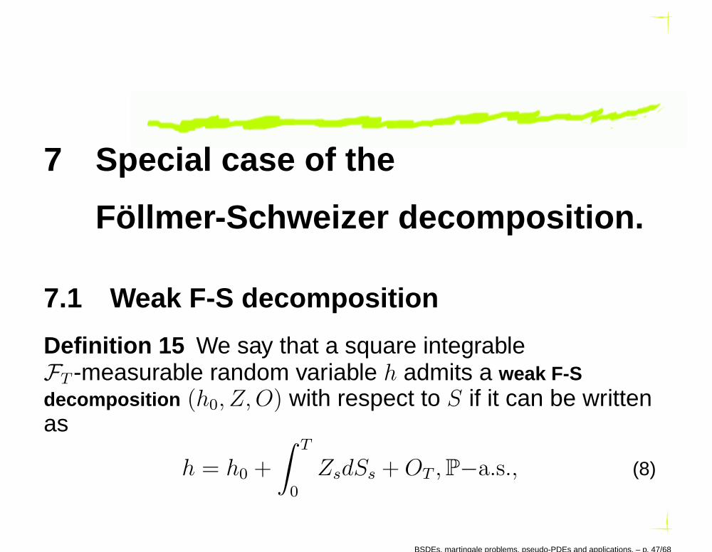
7.1 Weak F-S decomposition
Definition 15 We say that a square integrableFT -measurable random variable h admits a weak F-Sdecomposition (h0, Z,O) with respect to S if it can be writtenas
h = h0 +
∫ T
0
ZsdSs +OT ,P−a.s., (8)
BSDEs, martingale problems, pseudo-PDEs and applications. – p. 47/68
where h0 is an F0-measurable r.v., Z is a predictableprocess such that
∫ T
0|Zs|
2d〈MS〉s < ∞ a.s.,∫ T
0|Zs|d‖V
S‖s < ∞ a.s. and O is a local martingale suchthat 〈O,MS〉 = 0 with O0 = 0.
BSDEs, martingale problems, pseudo-PDEs and applications. – p. 48/68
7.2 Link to BSDEs
Finding a weak F-S decomposition (h0, Z,O) for some r.v.h is equivalent to provide a solution (Y, Z,O) of the BSDE
Yt = h−
∫ T
t
ZsdSs − (OT −Ot).
The link is given by Y0 = h0. Here the driver f is linear in z,of the form
f(t, x, s, y, z) = −A(id)(t, x, s)z.
⇒ The weak F-S decomposition can be linked to adeterministic problem (Pseudo-PDE).
BSDEs, martingale problems, pseudo-PDEs and applications. – p. 49/68
7.3 Weak Vs True F-S decomposition
Remark 16 Setting h0 = y(0, X0, S0), the triplet (h0, Z,O) isa candidate for a true F-S decomposition. Sufficientconditions for this are the following.
1. h = g(XT , ST ) ∈ L2(Ω).
2. (z(t,Xt−, St−))t ∈ Θ i.e.
E∫ T
0|z(t,Xt−, St−)|
2 A(id)(t,Xt−, St−)dAt < ∞.
E
(∫ T
0|z(t,Xt−, St−)| ‖A(id)(t,Xt−, St−)dA‖t
)2
< ∞.
3.(y(t,Xt, St)−
∫ t
0A(y)(u,Xu−, Su−)dAu
)t
is an
Ft-square integrable martingale.BSDEs, martingale problems, pseudo-PDEs and applications. – p. 50/68
Corollary 17 (Application of the theorem for general BSDEs)Let y (resp. z): [0, T ]×O → C. We suppose the following.
1. y, y := y × id belong to D(A).
2.∫ T
0z2(r,Xr−, Sr−)A(id)(r,Xr−, Sr−)dAr < ∞ a.s.
3. (y, z) solves the problem
A(y)(t, x, s) = A(id)(t, x, s)z(t, x, s),
A(y)(t, x, s) = A(id)(t, x, s)z(t, x, s),(9)
with the terminal condition y(T, ., .) = g(., .).
BSDEs, martingale problems, pseudo-PDEs and applications. – p. 51/68
Then the triplet (Y0, Z,O), where
Yt = y(t,Xt, St), Zt = z(t,Xt−, St−), Ot = Yt−Y0−
∫ t
0
ZsdSs,
is a weak F-S decomposition of h.
BSDEs, martingale problems, pseudo-PDEs and applications. – p. 52/68
7.4 Application 1: exponential of additive
processes
(X,S) = (eZ1
, eZ2
) is an exponential of additive processes.Example 18 Goal. Use the Pseudo-PDE to give explicitexpressions of a weak F-S of an FT -measurable randomvariable h of the form h := g(XT , ST ) for a function g of theform
g(x, s) =
∫
C2
dΠ(z1, z2)xz1sz2 ,
where Π is finite Borel complex measure.
BSDEs, martingale problems, pseudo-PDEs and applications. – p. 53/68
Existence and uniqueness.
Proposition 19 Suppose the validity of theBasic assumption and
∫ T
0
(dκt(0, 1)
dρSt
)2
dρSt < ∞.
Then any square integrable variable admits a unique trueF-S decomposition.The proof makes use of a general existence anduniqueness theorem by Monat and Stricker [1995].
BSDEs, martingale problems, pseudo-PDEs and applications. – p. 54/68
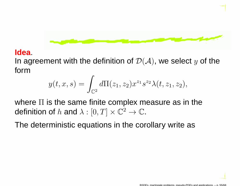
Idea.In agreement with the definition of D(A), we select y of theform
y(t, x, s) =
∫
C2
dΠ(z1, z2)xz1sz2λ(t, z1, z2),
where Π is the same finite complex measure as in thedefinition of h and λ : [0, T ]× C
2 → C.
The deterministic equations in the corollary write as
BSDEs, martingale problems, pseudo-PDEs and applications. – p. 55/68
∫
C2
dΠ(z1, z2)xz1sz2
dλ(t, z1, z2)
dρSt+ λ(t, z1, z2)
dκt(z1, z2)
dρSt
= sdκt(0, 1)
dρStz(t, x, s)
∫
C2
dΠ(z1, z2)λ(t, z1, z2)xz1sz2+1dρt(z1, z2, 0, 1)
dρSt= s2z(t, x, s)
y(T, ·, ·) = g.
Unknown : λ ⇒ can be determined through the resolutionof an ODE in t.
BSDEs, martingale problems, pseudo-PDEs and applications. – p. 56/68
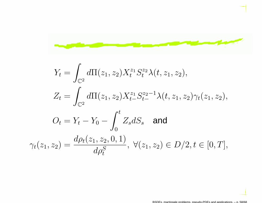
Theorem 20 (Weak F-S decomposition) Let λ be defined
as λ(t, z1, z2) = exp(∫ T
tη(z1, z2, du)
), ∀(z1, z2) ∈ D/2,
where
η(z1, z2, t) = κt(z1, z2)−
∫ t
0
dρu(z1, z2, 0, 1)
dρSuκdu(0, 1).
Then, under some technical assumptions, (Y0, Z,O) is a weakF-S decomposition of h, where
BSDEs, martingale problems, pseudo-PDEs and applications. – p. 57/68
Yt =
∫
C2
dΠ(z1, z2)Xz1t Sz2
t λ(t, z1, z2),
Zt =
∫
C2
dΠ(z1, z2)Xz1t−S
z2−1t− λ(t, z1, z2)γt(z1, z2),
Ot = Yt − Y0 −
∫ t
0
ZsdSs and
γt(z1, z2) =dρt(z1, z2, 0, 1)
dρSt, ∀(z1, z2) ∈ D/2, t ∈ [0, T ],
BSDEs, martingale problems, pseudo-PDEs and applications. – p. 58/68
Proposition 21 (True F-S decomposition) Under slightlystronger assumptions as in Theorem above, the weak F-Sdecomposition of
h =
∫
C2
dΠ(z1, z2)Xz1T Sz2
T
above is a true F-S decomposition.Moreover, if h is real-valued then the decomposition(h0, Z,O) is real-valued and it is therefore the unique F-Sdecomposition.Example 22 This statement is a generalization of theresults of [Oudjane, Goutte and Russo, 2014] to the caseof hedging under basis risk.
BSDEs, martingale problems, pseudo-PDEs and applications. – p. 59/68
7.5 Application 2: diffusion processes
Let (X,S) be a diffusion process with drift (bX , bS) andvolatility (σX , σS).
Assumption 23 bX , bS, σX and σS are continuous andglobally Lipschitz.
g : O → R is continuous.
BSDEs, martingale problems, pseudo-PDEs and applications. – p. 60/68
(X,S) solve the strong martingale problem related to(D(A),A, A) where At = t,D(A) = C1,2([0, T [×O) ∩ C1([0, T ]×O) and
A(y) = ∂ty + bS∂sy + bX∂xy
+1
2
|σS|
2∂ssy + |σX |2∂xxy + 2〈σS, σX〉∂sxy
,
A(y) = |σS|2∂sy + 〈σS, σX〉∂xy.
Example 24 Goal. characterize the (weak) F-Sdecomposition of h := g(XT , ST ).
BSDEs, martingale problems, pseudo-PDEs and applications. – p. 61/68
Theorem 25 (Weak F-S decomposition) We suppose thevalidity of Assumption 23. and that |σS| is always strictlypositive. If (y, z) is a solution of the system
∂ty +B∂xy +1
2
(|σS|
2∂ssy + |σX |2∂xxy + 2〈σS, σX〉∂sxy
)= 0,
y(T, ., .) = g(., .), where B = bX − bS〈σS, σX〉
|σS|2,
z = ∂sy +〈σS, σX〉
|σS|2∂xy,
(10)
BSDEs, martingale problems, pseudo-PDEs and applications. – p. 62/68
such that y ∈ D(A), then (Y0, Z,O) is a weak F-Sdecomposition of g(XT , ST ), where
Remark 26 1. Under slightly stronger assumption onecan give conditions for the existence of a trueFöllmer-Schweizer decomposition.
2. Black-Scholes was treated by Hulley and McWalter[2008].
BSDEs, martingale problems, pseudo-PDEs and applications. – p. 63/68
8 Extensions: BSDE vs Pseudo-PDE
Until now we have essentially shown that a solution toa blue Pseudo-PDE provide solutions to BSDEs driven bycadlag martingales.
More problematic is the converse implication.
Barrasso and Russo [2017a,b].
BSDEs, martingale problems, pseudo-PDEs and applications. – p. 64/68
Let E be a Polish space. Let Pt,x be a Markov class family ofprobability measures under which the canonical process Xon D([0, T ];E) solves a martingale problem to D(A),A, ρ).Let us denote MS := M id,t
s := Ss − x−∫ s
tA(id)(Sr)dρ(r).
We consider BSDE(f, g(ST ),M), i.e.
Ys = g(ST ) +
∫ T
s
f(r, Sr−, Yr−, Zr)dρr −
∫ T
s
ZrdMSr
(11)
− (OT −Os), s ∈ [t, T ],
under Pt,x.
BSDEs, martingale problems, pseudo-PDEs and applications. – p. 65/68
Let us suppose the following.
id ∈ D(A).
〈MS〉 is absolutely continuous with respect to ρ.
Let us suppose suitable growth condition on g andLipschitz on f .
BSDEs, martingale problems, pseudo-PDEs and applications. – p. 66/68
“Theorems”
Then (11) admits a unique solution (Y t,x, Zt,x, Ot,x) insome suitable spaces.
There is a “unique” couple (y, z) of Borel functions suchthat y(t, x) = Y t,x, and Zt,x
s = z(s,Xs) a.s. under Pt,x.
The couple (y, z) is a so called decoupled mild solution ofthe system.
There is a unique decoupled mild solution ofPseudo-PDE(f, g).
BSDEs, martingale problems, pseudo-PDEs and applications. – p. 67/68
Thank you for your attention!
BSDEs, martingale problems, pseudo-PDEs and applications. – p. 68/68
References
A. Barrasso and F. Russo. Backward Stochastic Differential
Equations with no driving martingale, Markov processes and