36
Bubble Plots as a Model- Free Graphical Tool for Three Continuous Variables and a Flexible R Function to Plot Them Keith A. Markus and Wen Gu John Jay College of Criminal Justice, CUNY
| Date post: | 19-Dec-2015 |
| Category: |
Documents |
| View: | 216 times |
| Download: | 0 times |

Bubble Plots as a Model-Free Graphical Tool for Three Continuous Variables
and a Flexible R Function to Plot Them
Keith A. Markus and Wen GuJohn Jay College of Criminal Justice,
CUNY


Overview
• Goal: Model-free graphs for 3 continuous variables.
• Some alternative graphs & design issues.• The R function: bp3way().• An empirical study.• Tentative conclusions & future directions.

The Goal
• The goal is to provide a useful graphical representation of the association between 3 continuous variables.
• Often: 2 IVs and 1 DV.• Model free:
– Exploratory data analysis. – Not a summary of a statistical model.

Why Model Free?
• If the statistical model is correct: model based graphs can be very efficient.
• If the statistical model is incorrect: model based graphs can be very misleading.
• E.g., Multiple y~x regression lines for values of z. Misleading if...– y~x relationship is not linear.– Variance in y varies with x or z.– Regression lines extrapolate beyond data.

Some Non-Options
• Scatterplot matrix.• y~x regression lines for fixed z values.• Factorial design type line plots.
• All good plots for other applications.• But not good plots for present purpose.

Scatterplot matrix
• Does not attempt to represent 3-way distributions.
• Same data used for all graphs (N = 100)

y~x regression lines for fixed values of z:
• Model dependent: plots model not data.
• Not clear where data leaves off.

Factorial-design type plots for categorized IVs:
• Model dependent (interpolation).
• Arbitrary cuts (quartiles plotted here).
• Loss of information through categorization.

Some Options• 3D Scatterplots.
– R Package scatterplot3d: scatterplot3()
• Co-plots.– R base installation: coplot()
• 3-way Bubbleplots.– Available from authors: bp3way()

3D scatterplot:• Natural extension of 2D scatter plot.
• Relies on 3D illusion: some ambiguity.

Co-plot
• Well suited to perceptual process.
• Relies on banding of z values.

3-Way Bubble Plot• 2D representation of 3D data.
• People tend to underestimate area.
• No literature.

Some Design Features of the 3-Way Bubble Plot
• Grid designed to make it easier to compare circle sizes across the plot surface.
• Shading designed to accentuate bubbles.• Limited number of cases plotted avoids overly
dense plots (in this case all 100 are plotted).• Margins avoid bubbles extending outside plot
region.

bp3way() function
Usagebp3way(x)
bp3way(x, xc=1, bc=2, yc=3, proportion=1, random=TRUE, x.margin=.1, y.margin=.1, rad.ex=1, rad.min=NULL, names=c('X', 'B', 'Y'), std=FALSE, fg='black', bg='grey90', tacit=TRUE, ...)

Data Parametersx is a data frame with at least 1 column.xc, yc, and bc identify the columns used to plot
the x axis, y axis, and bubbles respectively.names is a vector of variables names used in the
plot.• Easy to switch variables without changing the
data.• User can use same column more than once.• Out of bounds values return an error.

Data-sensitive Defaults Help Avoid Bad Plots

• Parameters with data sensitive defaults:– rad.ex: Radius expansion rate.– rad.min: Minimum bubble radius.– proportion: % of data plotted.– margins and grid.
• Other user-specified options include:– Plotting a random sample or first % of cases.– Standardization of X and Y variables.– labels and colors.

Empirical Study• 3 Plots (Bubbleplot, 3D Scatterplot, Coplot).
– Between subjects.– Within group n = 36.
• 6 Data sets.– Within subjects.
• N of subjects = 108.• N of observations = 108 x 6 = 648.

Four DVs
• Accuracy of interpretation of graphs– 0-3 questions answered correctly.
• Confidence in interpretation– 1-5, average of 3 1-5 Likert scale items.
• Perceived clarity– 1-5 Likert scale item.
• Perceived ease of use– 1-5 Likert scale item.

Univariate Summary• No floor or ceiling effects, variability in DVs.

Correlations Between Outcomes
Accuracy Confidence Clarity Ease of Use
Accuracy 1 .061 -.058 -.102
Confidence .106 1 .497 .471
Clarity -.118 .586 1 .784
Ease of Use -.115 .562 .866 1
• Above Diagonal: N = 648 observations.• Below Diagonal: N = 108 participants.

Multivariate model fit firsty* = α0 + α1' Data + α2' Data Graph∙ + u1 (Level 1)
α 0 = β0 + β1' Graph + u2 (Level 2)
y = { 0 if y* ≤ τ1, 1 if τ 1 < y* ≤ τ 2, ... k if τ k-1 < y* ≤ τ k} (Threshold model)
• Third equation not used for confidence DV.• Full model: Mplus• Confidence also fit in R using lme() function.• Nearly identical estimates with R or Mplus.• Story in interactions, not main effects.

Follow-up: Simple Effects
• Shift focus to simple effects because we cannot usefully interpret interactions.
• Protected Wilcox Mann Whitney Exact Tests Used for Accuracy, Clarity and Ease of Use DVs.
• Protected t tests used for Confidence DV.• No one graph consistently better.• Mostly a story about accuracy.
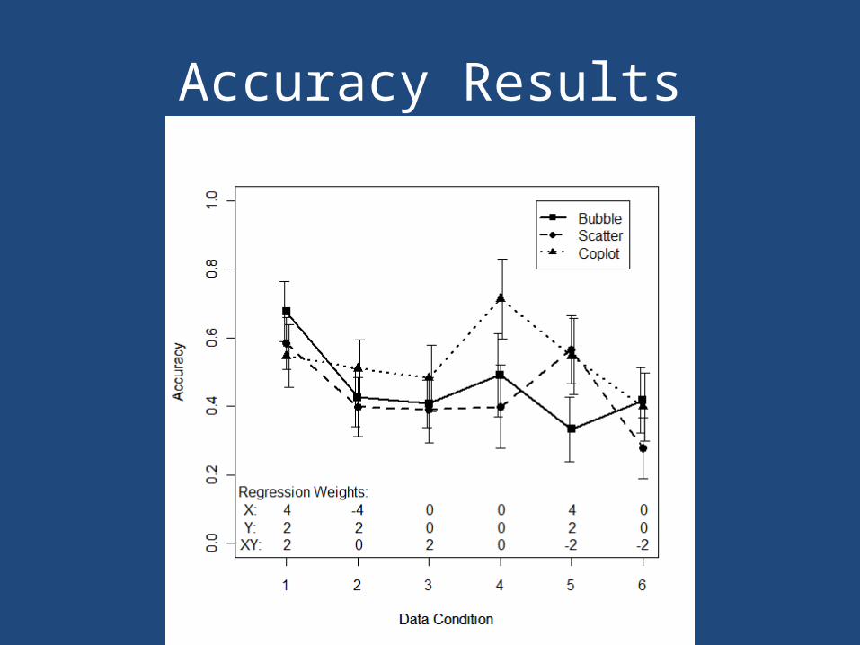
Accuracy Results

Accuracy Results

Confidence Results

Confidence Results

Perceived Clarity Results

Perceived Clarity Results

Perceived Ease of Use Results

Perceived Ease of Use Results

Tentative Conclusions
• Much remains to be learned about the cognition of these 3 graph types.– Coplot may have a slight edge over the other two.– But optimal plot seems data dependent.– Study included a limited range of data and graph
conditions.– More detailed perceptual theory is needed to
optimize graph design.

• Recommendation for exploratory analysis:– Use 2 or more graph types.– Cannot predict ahead of time which will work
best.– Probably useful to look at data more than one
way even if one graph were consistently best.

• Recommendation for reporting results:– Use model based graphs.
• If you understand your data well enough to fit a good model.
– If not, try different model-free graphs and see which seems to work best.
Future Directions
• Identify factors that impact which graph works best.
• Identify design factors that maximize effectiveness of all 3 graph types.
• Increase statistical power:– Identify individual difference covariates that
account for within condition variance.– More sensitive outcome measures.


