Page 1
Buckling Analysis of Partially Free Standing Piles in
Non-homogenous Soil Medium under Pure Scour Effect
By
Culture Atika
U1153012
A dissertation submitted in partial fulfilment of the requirements for the degree of:
Master of Science in
Civil Engineering
Submitted to the University of East London
On
27 September 2013
Supervisor: Dr Hamid Z. Jahromi
Page 2
i
ABSTRACT
Scour is a form of erosion that occurs around marine structures or structures in
coastal environment. It has been found by previous research that scour reduces
the buckling capacity of a pile and it is also known to cause failure such as
differential settlement, tilting and overturning to mention but a few.
To date the study of the effect of scour on the buckling capacity of piles has
been either general or limited to scour around bridge piers. This study looks at a
purely scour condition on the buckling capacity of partially free standing piles
either as a monopile or in a group of piles affected by group action.
Using the Winkler type (a system of mutually independent linear springs)
mathematical model to represent the pile-soil interaction the buckling capacity
of the piles are determined via finite element method with the aid of a computer
software (StaadPro) for varying scour depth and for different sand densities
(loose, medium and dense sand). Also the buckling capacity is determined
considering varying pile head stiffness assuming full fixity of the pile tip.
It is found that scour does significantly reduce the buckling capacity of partially
free standing piles. The reduction was very significant upto 44% for 70cm piles
in groups affected by group action. It was less significant for partially free
standing piles classified as monopiles 3.5% for the 30cm monopile and about
10% for the 70cm monopile. Also, results show that the sand density did not
create any significant change in the buckling capacity of the piles. However,
variation in pile head stiffness did affect the buckling capacity significantly.
The study does provide evidence that scour significantly reduces the buckling
capacity of piles in groups affected by group action. It also shows that the
reduction may be classified as insignificant for piles of small diameter less than
40cm for piles that could be referred to as monopiles. On the other hand it does
show that the reduction increases with diameter and upto 44% reduction in the
buckling capacity of the 70cm pile in the group affected by group action.
Page 3
ii
ACKNOWLEDGEMENT
My thanks go first to God Almighty for His Grace that has enabled me to
complete this dissertation successfully. This acknowledgement will not start of
properly without mentioning Dr Hamid Z. Jahromi, my supervisor to whom there
is no like. He came at a time when I was weary and tired of writing dissertation
proposals; he helped set the part straight and his guidance throughout this
period can never be overlooked. Many thanks to senior colleagues in this field
of research, the authors of ‘’p-y Approach to Analysing Buckling of Axially
Loaded Piles in Scoured Condition’’, who made their work available to me for
free and to those authors I have referenced in this dissertation for their works.
My thanks to the jewel of my life who with tears in her eyes accosted me to the
place of saying good bye, to journey to a place foreign to us. An opportunity
cost at the time for her hugs and kisses; yet in almost two years still very
supportive of this cause of an MSc. I thank you for your undoubting love and
patience. It is with gratefulness to God Almighty that I express an inexpressible
thanks to the family of Mr David Kamara, who has always been there for me; for
shelter and for provision; as a friend and as a family; one love brother. My
thanks to Miss Blessing Campbell who out of time took time to help me
acclimatise in the city called London.
This acknowledgement section will not be complete without mentioning the
support and love from my family members. My dad and mum, Mr and Mrs Atika
and siblings, Efe, Serome, Ejogbamu and Edesiri all Atika’s whom have been
constantly sharing their love from abroad and constantly supporting this cause.
Also many thanks to my academic friends a list too numerous to mention;
Kwabena Osei-bonsu; David D. Appah; Benjamin Appah; Tarila Tebepah and
Utoejit A. Bara. This last line have I kept for those with whom in one faith I am
connected; Rev. Prosper Idjesa and family; Pastor Friday and Family and the
membership of their flocks may God bless you all for your prayers and support.
Page 4
Table of Contents
CHAPTER 1. INTRODUCTION .................................................................................................... 1
1.1 BACKGROUND ................................................................................................................ 1
1.2 PROBLEM STATEMENT AND SIGNIFICANCE ....................................................................... 1
1.3 RESEARCH QUESTION .................................................................................................... 3
1.4 AIMS AND OBJECTIVES............................................................................................. 4
1.4.1 Aim ........................................................................................................................... 4
1.4.2 Objectives ................................................................................................................ 4
CHAPTER 2. PILES ...................................................................................................................... 5
2.1 INTRODUCTION ............................................................................................................... 5
2.2 DEFINITION .................................................................................................................... 5
2.3 WHEN TO USE PILES ...................................................................................................... 5
2.4 CLASSIFICATION OF PILES .............................................................................................. 6
2.5 ANALYSIS OF PILES ........................................................................................................ 8
2.5.1 Driving Formulae ..................................................................................................... 9
2.5.2 Soil Mechanics Expressions .................................................................................. 10
2.6 BUCKLING ANALYSIS .................................................................................................... 11
2.7 SUMMARY .................................................................................................................... 13
CHAPTER 3. SCOUR ................................................................................................................. 14
3.1 INTRODUCTION ............................................................................................................. 14
3.2 DEFINITION .................................................................................................................. 14
3.3 DISCREPANCIES IN SCOUR IDEOLOGY BY PICTURES WITH PARTICULAR REFERENCE TO
PILES 15
3.4 TYPES OF SCOUR ......................................................................................................... 16
3.4.1 Clear Water Scour: ................................................................................................ 16
3.4.2 Contraction Scour: ................................................................................................. 17
3.4.3 General Scour: ...................................................................................................... 17
3.4.4 Local Scour: ........................................................................................................... 17
3.4.5 Global Scour: ......................................................................................................... 18
3.5 HYDRODYNAMIC CONDITION FOR SCOUR FORMATION .................................................... 19
3.6 IMPACTS OF SCOUR ON FOUNDATIONS .......................................................................... 20
3.7 ESTIMATION OF SCOUR DEPTH ..................................................................................... 21
3.7.1 Scour Depth around Piles...................................................................................... 21
3.7.2 Scour Depth around Abutments ............................................................................ 24
3.7.3 Failures Caused by Scour ..................................................................................... 26
3.8 SUMMARY .................................................................................................................... 27
CHAPTER 4. BUCKLING IN PILES ........................................................................................... 28
4.1 INTRODUCTION ............................................................................................................. 28
Page 5
4.2 BUCKLING .................................................................................................................... 28
4.2.1 Euler Buckling Load ............................................................................................... 29
4.3 BUCKLING ANALYSIS OF PILES ...................................................................................... 31
4.3.1 Davisson’s Method ................................................................................................ 31
4.3.2 Davisson’s and Robinsons Approach .................................................................... 32
4.3.3 Finite Difference Method ....................................................................................... 33
4.3.4 Finite Element Method ........................................................................................... 34
4.4 SUMMARY .................................................................................................................... 35
CHAPTER 5. SOIL-STRUCTURE INTERACTION .................................................................... 36
5.1 INTRODUCTION ............................................................................................................. 36
5.2 DEFINITION .................................................................................................................. 36
5.2.1 Winkler Model ........................................................................................................ 37
5.2.2 Elastic Continuum Model ....................................................................................... 43
5.3 SUMMARY .................................................................................................................... 44
CHAPTER 6. RESEARCH METHOD ......................................................................................... 45
6.1 OVERVIEW ................................................................................................................... 45
6.2 SAMPLE DESCRIPTION .................................................................................................. 45
6.2.1 Pile: ........................................................................................................................ 45
6.2.2 Scour Depth: .......................................................................................................... 45
6.2.3 Soil Stiffness: ......................................................................................................... 45
6.2.4 Mathematical Model: ............................................................................................. 46
6.2.5 Software:................................................................................................................ 47
6.3 PROCEDURE: ............................................................................................................... 47
CHAPTER 7. VERIFICATION .................................................................................................... 49
7.1 OVERVIEW ................................................................................................................... 49
7.2 EULER BUCKLING LOAD THEORY................................................................................... 49
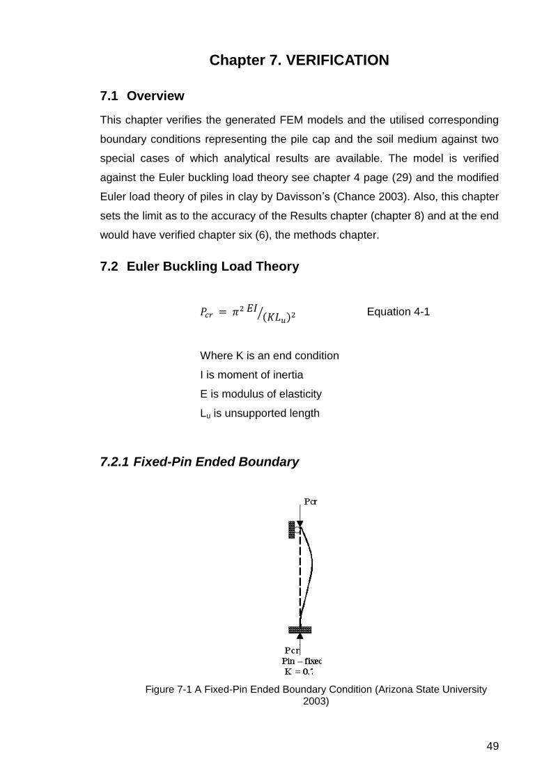
7.2.1 Fixed-Pin Ended Boundary.................................................................................... 49
7.2.2 Fixed-Fixed Ended Boundary ................................................................................ 51
7.2.3 Pinned-Pinned Boundary Condition ...................................................................... 52
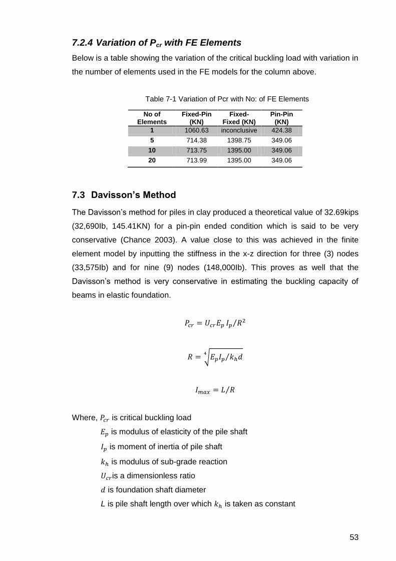
7.2.4 Variation of Pcr with FE Elements .......................................................................... 53
7.3 DAVISSON’S METHOD ................................................................................................... 53
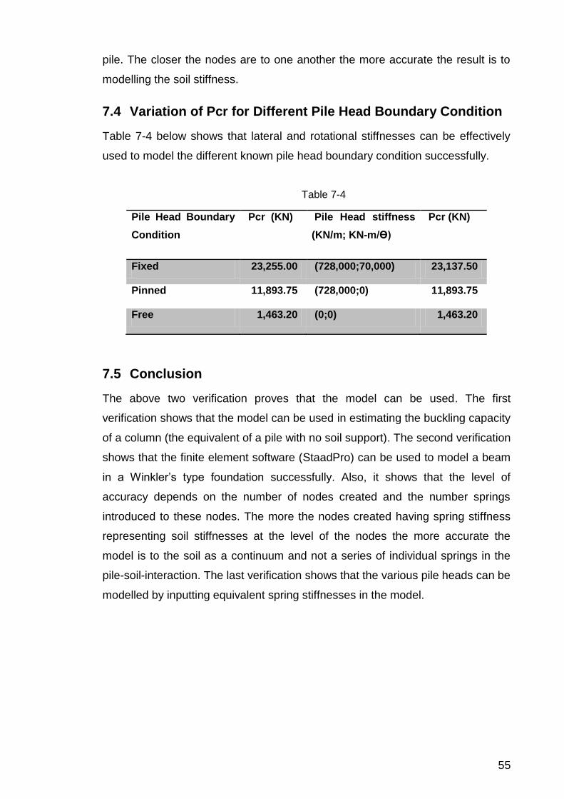
7.4 VARIATION OF PCR FOR DIFFERENT PILE HEAD BOUNDARY CONDITION .......................... 55
7.5 CONCLUSION ............................................................................................................... 55
CHAPTER 8. RESULTS ............................................................................................................. 56
8.1 OVERVIEW ................................................................................................................... 56
8.2 VARIATION OF BUCKLING STRENGTH WITH NORMALISED SCOUR DEPTH ......................... 57
8.2.1 Monopiles .............................................................................................................. 57
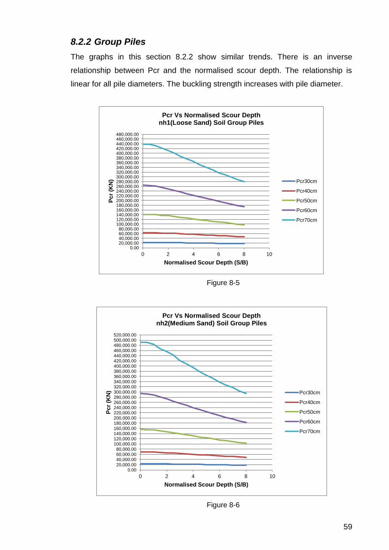
8.2.2 Group Piles ............................................................................................................ 59
Page 6
8.3 VARIATION OF PCR WITH NORMALISED SCOUR DEPTH FOR DIFFERENT SOIL CONDITION
FOR 30CM PILE .......................................................................................................................... 60
8.3.1 Monopile ................................................................................................................ 60
8.3.2 Group Piles ............................................................................................................ 61
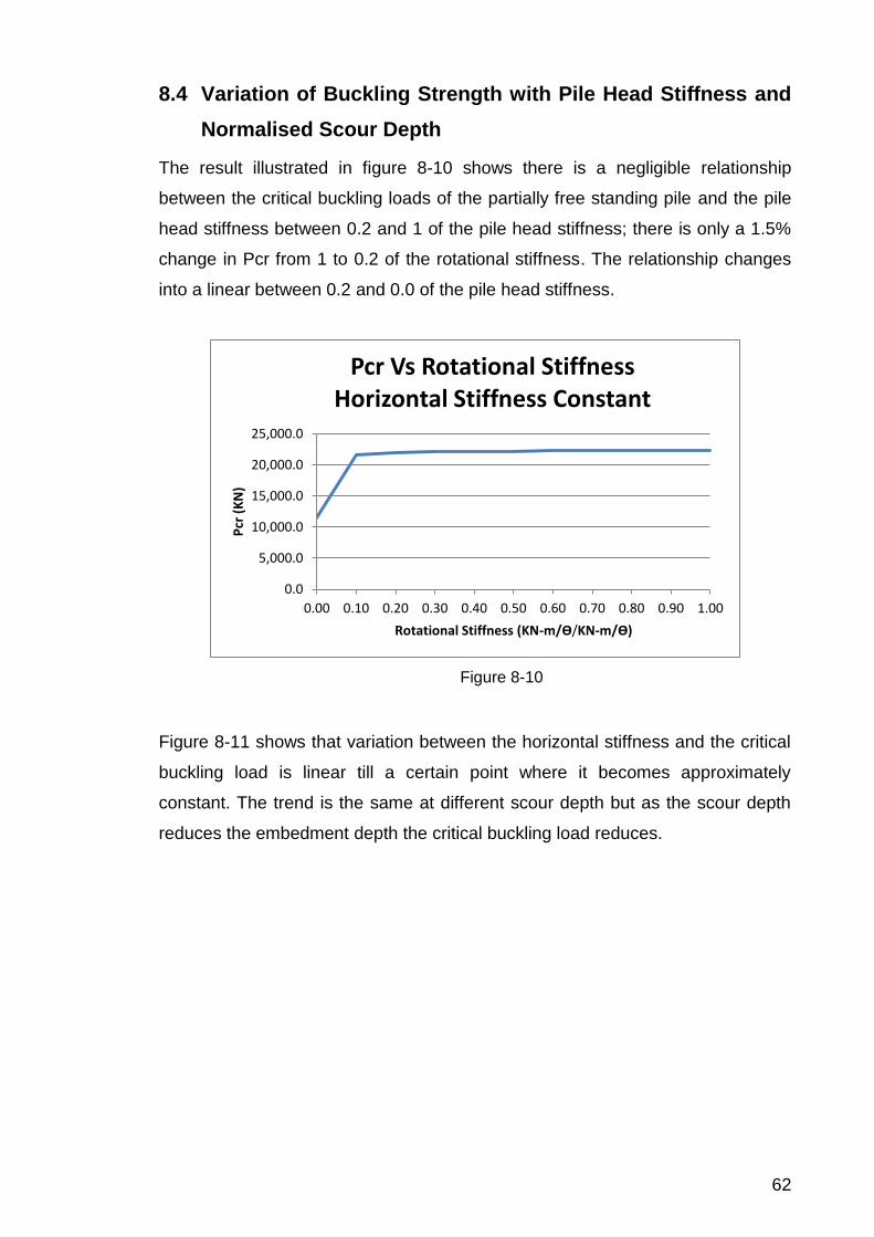
8.4 VARIATION OF BUCKLING STRENGTH WITH PILE HEAD STIFFNESS AND NORMALISED SCOUR
DEPTH 62
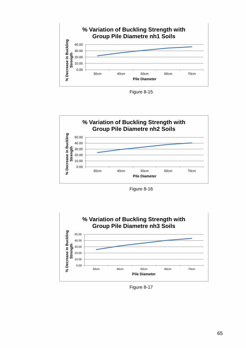
8.5 PERCENTAGE VARIATION OF BUCKLING STRENGTH AT MAXIMUM SCOUR DEPTH FOR
DIFFERENT PILE DIAMETRES ...................................................................................................... 63
8.5.1 Monopiles .............................................................................................................. 63
8.5.2 Group Piles ............................................................................................................ 64
CHAPTER 9. DISCUSSION ....................................................................................................... 66
9.1 OVERVIEW ................................................................................................................... 66
9.2 VARIATION OF BUCKLING STRENGTH WITH NORMALISED SCOUR DEPTH ......................... 66
9.3 VARIATION OF PCR WITH NORMALISED SCOUR DEPTH FOR DIFFERENT SOIL CONDITION
FOR 30CM PILE .......................................................................................................................... 66
9.4 VARIATION OF BUCKLING STRENGTH WITH PILE HEAD STIFFNESS................................... 67
9.5 PERCENTAGE VARIATION OF BUCKLING STRENGTH AT MAXIMUM SCOUR DEPTH FOR
DIFFERENT PILE DIAMETRES ...................................................................................................... 68
CHAPTER 10. CONCLUSION .................................................................................................... 69
10.1 OVERVIEW ................................................................................................................... 69
10.2 AIMS ............................................................................................................................ 69
10.3 FINDINGS ..................................................................................................................... 69
10.4 SIGNIFICANCE .............................................................................................................. 70
10.4.1 Significance of Findings .................................................................................... 71
10.5 LIMITATIONS ................................................................................................................. 71
10.6 RECOMMENDATION FOR FURTHER WORK ...................................................................... 71
10.7 CONCLUSION ............................................................................................................... 71
APPENDIX A ................................................................................................................................. I
APPENDIX B ............................................................................................................................... III
Page 7
List of Figures
Figure 1-1 Scoured Pile ................................................................................................................ 3
Figure 2-1 Classification of Piles BSi, (1986) ................................................................................ 8
Figure 2-2 Partially Embedded Pile ............................................................................................. 12
Figure 2-3 Practical Consideration of Pile Unsupported Length Chance, (2003) ....................... 12
Figure 3-1 Scour around Single Pile Figure 3-2Scour in Pile Group .................................... 15
Figure 3-3 Scour in Pile Group in a Bridge Figure 3-4 Pile Group Affected by Erosion ........... 15
Figure 3-5 Pictorial Representation of the Difference between Scour and Erosion ................... 16
3-6 Local Scour around a Single Pile Federal Emergency Management Agency (FEMA), (2011)
............................................................................................................................................ 17
3-7 Scour in a Pile Group (Federal Emergency Management Agency (FEMA) 2011) ............... 18
Figure 3-8 Formation, Physical Processes http://www.usgs.gov/ ............................................... 20
3-9 Local Scour in a Pile Group without Group Interaction ......................................................... 21
Figure 3-10 Abutment Failure Caused by Scour ......................................................................... 26
Figure 3-11 Differential Settlement Caused by Scour ................................................................. 26
Figure 4-1 The Concept of Effective Length of Slender Column/Pile (Bhattacharya & Bolton,
2004) ................................................................................................................................... 30
Figure 4-2 Poulos and Davis 1980 as cited by (Chance, 2003) ................................................. 32
Figure 5-1 Soil Structure-Interaction ........................................................................................... 37
Figure 5-2 Winkler's Beam on Elastic Foundation ...................................................................... 38
Figure 5-3, Axial and Transversely Loaded Beam-Column on Soil ............................................ 38
Figure 5-4 A Graph of Coefficient of Subgrade Reaction ........................................................... 40
Figure 7-1 A Fixed-Pin Ended Boundary Condition (Arizona State University 2003) ................. 49
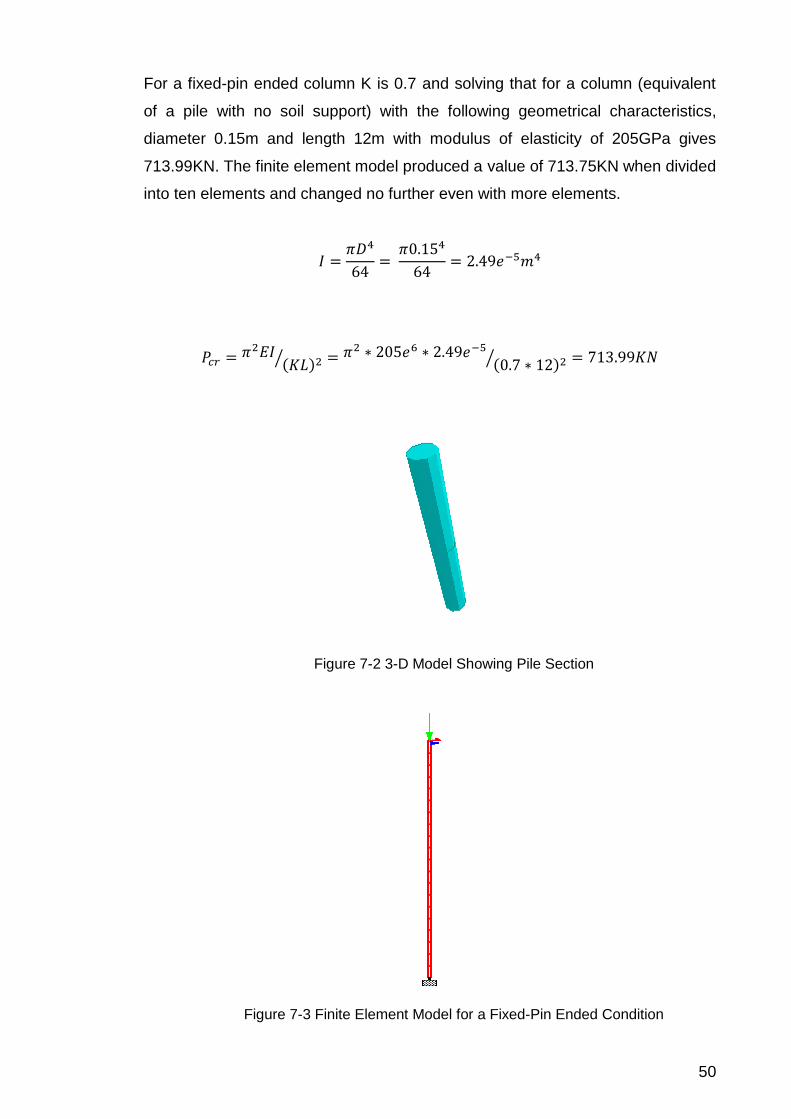
Figure 7-2 3-D Model Showing Pile Section ............................................................................... 50
Figure 7-3 Finite Element Model for a Fixed-Pin Ended Condition ............................................. 50
Figure 7-4 Fixed-Fixed Boundary Condition (Arizona State University 2003) ............................ 51
Figure 7-5 FE Model for a Fixed-Fixed Boundary Condition....................................................... 51
Figure 7-6 Pinned-Pinned Boundary Condition (Arizona State University 2003) ....................... 52
Figure 7-7 FE Model for Pinned-Pinned Boundary Condition ..................................................... 52
Figure 7-8 The Finite Element Model .......................................................................................... 54
Figure 8-1 Figure of the Finite Element Model ............................................................................ 56
Figure 8-2 .................................................................................................................................... 57
Figure 8-3 .................................................................................................................................... 58
Figure 8-4 .................................................................................................................................... 58
Figure 8-5 .................................................................................................................................... 59
Figure 8-6 .................................................................................................................................... 59
Figure 8-7 .................................................................................................................................... 60
Figure 8-8 .................................................................................................................................... 61
Figure 8-9 .................................................................................................................................... 61
Figure 8-10 .................................................................................................................................. 62
Figure 8-11 .................................................................................................................................. 63
Figure 8-12 .................................................................................................................................. 63
Page 8
Figure 8-13 .................................................................................................................................. 64
Figure 8-14 .................................................................................................................................. 64
Figure 8-15 .................................................................................................................................. 65
Figure 8-16 .................................................................................................................................. 65
Figure 8-17 .................................................................................................................................. 65
Figure A-1 Quantitative Process for Estimating Total Scour Depth (Coleman & Melville 2001) .... i
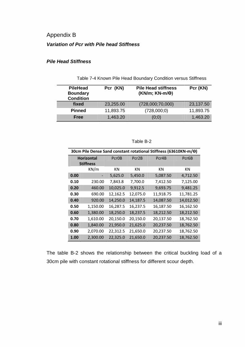
Figure B-2 (Cheng et al. 2010) ...................................................................................................... iv
List of Tables
Table 5-1 Values of ks1 (KN/m3) for 1ft square plate on sand (Terzaghi 1955) ......................... 41
Table 5-2 Ks1 values (KN/m3) for pre-compressed clay (Terzaghi 1955) .................................. 42
Table 5-3 and values for Sand (Terzaghi 1955) ................................................................ 42
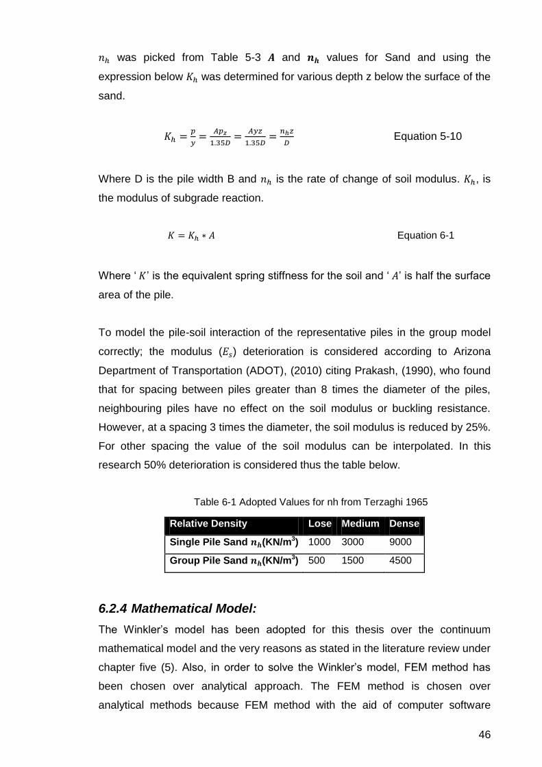
Table 6-1 Adopted Values for nh from Terzaghi 1965 ................................................................ 46
Table 7-1 Variation of Pcr with No: of FE Elements .................................................................... 53
Table 7-2 Pile Properties ............................................................................................................. 54
Table 7-3 Variation of Pcr with No: of Nodes having Spring Stiffness ........................................ 54
Table 7-4 ..................................................................................................................................... 55
Table A-1 Normalised Scour Depth S/B from Literature Review ................................................... ii
Table B-2 ....................................................................................................................................... iii
Page 9
List of Symbols and Meaning
area of the pile base
total surface area of the pile shaft
and are coefficients calculated from
pile diameter
total temporary compression of piles
foundation shaft diameter
the size of the grain at the bed around the pile
the diameter of the pile
secant modulus
modulus of elasticity of the pile shaft
a product of the modulus of elasticity and moment on inertia
soil rigidity per unit length
Frouds number
the design ultimate pile carrying capacity
height of fall of hammer or water depth
moment of inertia of pile shaft
an end condition
pile shape factor or the correction factor for abutment shapes
pile orientation factor or is the correction factor for the abutment
alignment to flow
linear elastic stiffness matrix
KC Keulegan Carpenter number
modulus of sub-grade reaction
the total stiffness of a beam on an elastic foundation
L pile shaft length over which is taken as constant
unsupported length of the strut or pile
efficiency of blows found from graph
the Euler’s critical buckling load of an axially loaded strut
ultimate bearing capacity of the pile
the ultimate base resistance
the ultimate shaft resistance
base bearing capacity
shear strength of the soil
Page 10
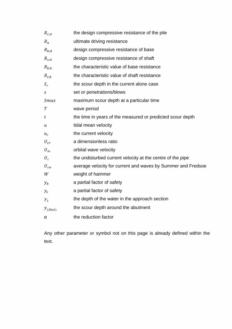
the design compressive resistance of the pile
ultimate driving resistance
design compressive resistance of base
design compressive resistance of shaft
the characteristic value of base resistance
the characteristic value of shaft resistance
the scour depth in the current alone case
set or penetrations/blows
maximum scour depth at a particular time
wave period
the time in years of the measured or predicted scour depth
tidal mean velocity
the current velocity
a dimensionless ratio
orbital wave velocity
the undisturbed current velocity at the centre of the pipe
average velocity for current and waves by Summer and Fredsoe
weight of hammer
a partial factor of safety
a partial factor of safety
the depth of the water in the approach section
the scour depth around the abutment
α the reduction factor
Any other parameter or symbol not on this page is already defined within the
text.
Page 11
1
Chapter 1. INTRODUCTION
1.1 Background
Structural safety is the hallmark of civil engineering and ambiguity in any aspect
of the fields of civil engineering does not help this cause. However, where there
is an ambiguity it is only proper for a definition of a particular problem sort to be
solved and a definition of the solution provided be made explicit to cure up any
such ambiguity as to the ones that have existed. It is in this light this dissertation
has sort to look into the problem of the buckling analysis of partially free standing
pile under pure scour effect.
Researchers in time past have presented different literatures from studies as to
what scour is and what scour is not (Agrawal, Khan & Yi 2007), (Fayazi &
Farghadan 2012), (Seung, Briaud & Chen 2010) etc. Scour has been defined as
a form of erosion that occurs locally around a structure and caused by the
presence of the structure. However, where more than a majority of researchers
agree with this definition deviations have been noticed in the methods of
analysis. Many researchers treat a general degradation of the bed of the water
course mixed with a scour event as a scour event instead of an erosion event
whereas other researchers treat this as an erosion event. A scour event is an
event that does not involve the general degradation of the water bed but a
degradation caused by the presence of a structure in the water bed.
Partially free standing piles are piles that are not completely embedded into the
ground. It is believe that the formation of scour around them can pose an
instability problem as it reduces the depth of embedment and increases the
unsupported length.
1.2 Problem Statement and Significance
The problem this thesis is attempting to address is a reduction in confining
pressure as a result of reduction in depth of embedment caused by scour
formation around partially free standing piles. This thesis tries to ascertain if this
reduction in depth of embedment caused by scour around piles is enough to
Page 12
2
cause a significant decrement in the buckling capacity of affected piles whether
in water or shore line environment.
This thesis models a single partially free standing pile under scour effect and a
single representative partially free standing pile in a group under scour effect and
performs a buckling analysis on each sample pile considering varying scour
depth till the maximum scour depth. Using Winkler’s hypotheses i.e. a system of
mutually independent linear springs, this literature models the soil-pile interaction
via Finite Element Method (FEM) using StaadPro software. This thesis has by
way of literature review determined the maximum sample scour depth used in
the analysis.
What distinguishes this research from others is that it looks into buckling analysis
of partially free standing piles under scour effects caused by the pile-water
interaction without any external influence. This research does not include scour
around piles caused by a contraction of the river channel resulting in contraction
scour and its likes. This research includes scour around piles in off-shore
structures and river basin structures such as platforms and houses mounted on
piles. If there is a global scour, it is only of those caused by the pile group action
without any other structural interference. This research also has not attempted to
solve the problem from a generic point of view but has distinguished between
two types of piles monopiles and group piles. By this a much succinct view of the
problem is created and a better method of analysis may be provided.
The significance of this research is that for the first time the study of pile
behaviours under scour effect has been separated to partially free standing
monopiles and pile groups affected by scour caused by their own interaction with
the water flow and without any external interference. Also, in its revelation an
engineer may be confident as to how to approach this sort of problem.
Page 13
3
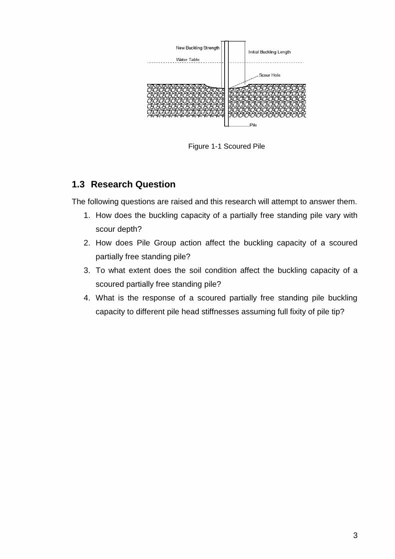
Figure 1-1 Scoured Pile
1.3 Research Question
The following questions are raised and this research will attempt to answer them.
1. How does the buckling capacity of a partially free standing pile vary with
scour depth?
2. How does Pile Group action affect the buckling capacity of a scoured
partially free standing pile?
3. To what extent does the soil condition affect the buckling capacity of a
scoured partially free standing pile?
4. What is the response of a scoured partially free standing pile buckling
capacity to different pile head stiffnesses assuming full fixity of pile tip?
Page 14
4
1.4 AIMS AND OBJECTIVES
1.4.1 Aim
The aim of this research is to model the effect of scour on axially loaded partially
free standing piles.
1.4.2 Objectives
My objectives are to:
Determine the extent to which scour can be formed around a pile by
looking at previous studies.
To model pile-soil interaction at varying and the maximum scour depth
using a system of mutually independent springs (Winkler type)
representing the non-homogenous soil medium via Finite Element Method
(FEM).
Determine the buckling response for the above pile-soil coupled under
different soil conditions loose, medium and dense sand (nh1, nh2 and
nh3)
Determine the buckling response for the above pile-soil coupled system
under varying boundary stiffnesses for the pile head.
Also, critically analyse and discuss the results.
Page 15
5
Chapter 2. PILES
2.1 Introduction
This chapter explains briefly what piles are and talks about pile classification.
Also, it describes briefly the main methods of analysing piles. At the end of the
chapter the reader should know what piles are and also be able to classify and
analyse them.
2.2 Definition
Piles are foundations used when a structure cannot be safely supported on a
shallow foundation. A single pile can be defined as a long structural element that
is used to transfer loads applied at the top through the base to the lower grounds
(University of Bolton, 2010). According to Sew & Meng, (2009), pile is a
foundation system that transfers load to a deeper and competent layer of the
soil. The authors all say the same thing about pile, as a foundation and carries
load from the superstructure into the lower but more solid layer of the ground
able to bear the load.
Piles carry their loads by means of:
Skin friction in sands or adhesion in clay: This is the shear force mobilised
on the surface of the shaft of the pile.
Bearing capacity at the end or tip of the pile (University of Bolton, 2010)
2.3 When to Use Piles
In her lecture note University of Bolton, (2010) said piles can be used under the
following listed conditions:
Where the soil layer of satisfactory bearing capacity lies too deep for
conventional or shallow footing to be applied economically.
Where the nature of the soil immediate underlying a structure is
moderately or highly variable.
Where the soil strata are deeply inclined and in some case the ground
surface as well.
In places of poorly compacted soil or soft soil immediately underlying a
structure.
Page 16
6
On a shore line or in the river where the effect of scouring and wave can
vary the amount of material at the surface. The buckling analysis of piles
under this condition is the centre issue of this research.
To transmit structural highly concentrated loads.
For structures that may be highly sensitive to differential settlement.
Also, for structures transmitting high amount of horizontal or inclined
loads.
Also, Sew & Meng, (2009) piles can be used to take care of inadequate bearing
capacity of shallow foundations; prevent uplift forces and to reduce excessive
settlements.
2.4 Classification of Piles
Piles can be classified University of Bolton, (2010) according to design or
construction method as:
Driven or Displacement Piles: These are preformed piles. They are driven,
screwed or hammered into the ground.
Bored or Replacement Piles: These require holes to be bored into the
crust before they are casted or formed in the holes usually of reinforced
concrete.
According to Geotechnical Engineering Office, (2006) piles can be classified
according to the type of material they are made of; mode of transmitting the
applied load; the degree of soil or ground displacement during installation and by
the method of installation. They believe that pile classification according to
material type has its drawback as there are not only steel, wooden or concrete
piles but composite piles. However, there are other researchers and the codes of
practice that do not see this as a problem.
Though Sew & Meng, (2009) and the various codes of practice British Standsrd
Institute (BSi), (2004) etc, classified piles under two classes as among other
classes as friction piles (piles resisting load mainly by the mobilised shear stress
on the shaft surface) and end bearing piles (piles resisting load mainly by the
load bearing resistance derived from the base); Geotechnical Engineering Office,
(2006) believes this method of classification by load transfer is very hard to set
Page 17
7
up as the shaft resistance and end bearing capacity cannot be reliably predicted
in practice.
According to Geotechnical Engineering Office, (2006), during the installation of
piles, either displacement or replacement is more predominant than any other
factor considered in the classification of piles. This ideology was drawn from
BS8004 which this research has also looked into. As classified by BS8004 BSi,
(1986) piles may be divided into three types depending on their effect on the soil.
The classification is as follows:
Large Displacement Piles: these piles include all solid piles, timber,
precast concrete and steel. It also includes concrete tubes closed at the
lower end with shoe or plug which may be left in position or extruded to
form an enlarged foot.
Small displacement Piles: this class includes rolled steel sections such as
H piles; open ended tubes and hollow section if the ground or soil enters
freely during driving installation. However, open ended tubes and hollow
sections frequently get plugged and become displacement piles. The H
pile also, behaves like this.
Replacement Piles: This class of piles are formed majorly by boring or
other methods of excavations. The excavation or borehole is lined with a
casing or tube that is either left in place or extracted as the hole is filled.
According to Geotechnical Engineering Office, (2006) there is also the class
called special piles.
Special Piles: these are particular pile types or variant of existing pile
types created in order to improve efficiency or cater for certain ground
conditions. There are three major special pile types; shaft and base
grouted piles; jacked piles and Composite piles.
Page 18
8
Figure 2-1 Classification of Piles BSi, (1986)
2.5 Analysis of Piles
For the analysis or design of load bearing piles part 5 of Euro code 3 refers to
part 1 of Euro code 7. For load bearing piles under compression which is
considered only in this literature, Euro code 7 provides the following.
To demonstrate that under compressive load the pile foundation will not
fail for all ultimate limit state load cases and combinations.
Equation 2-1
In principle should include the self weight of the pile and the
overburden pressure of the soil. These items should be disregarded if
they cancel out approximately.
For all other guidance for the design or analysis of pile see Euro code 7 part 1.
Page 19
9
The analysis of pile foundation is a rather complex task and there are two major
approaches to the design of a pile (University of Bolton 2010).
Pile carrying capacity estimation from driving formula and load test. This is
only suitable for sands/gravels or stiff clay and
Carrying capacity estimation from soil mechanics expressions.
2.5.1 Driving Formulae
There are loads of expressions and are all trying to relate the energy needed to
drive the pile to its penetration and to which there is no scientific proof.
E.g. Hiley’s formula
Equation 2-2
Where Ru is ultimate driving resistance
W is weight of hammer
h is fall of hammer
n is efficiency of blow found from graph
s is set or penetrations/blows
c is total temporary compression of piles.
The inadequacy of the driving formula is not farfetched as it takes no account of
the nature of the soil and for this a lot of structural engineers are in
disagreement. According to University of Bolton, (2010) the only sure way is to
drive some piles and then carry a load test to determine the carrying capacity.
This cost time and money. British Standsrd Institute (BSi), (2004), provides that
the pile driving formula should only be used if the following conditions are
satisfied:
If the stratification of the soil in which pile will be embedded has been
determined.
If the validity of the formula has been tested before with experimental
evidence of satisfactory performance on static load test of same pile type,
of similar cross section, material and similar ground condition.
Page 20
10
For end bearing piles in non-cohesive soil the value of the design
compressive resistance shall be determined according to clause 7.6.2.4
(ultimate compressive resistance from dynamic impact test)
If the pile driving test is carried on at least five piles distributed with
sufficient spacing in the piling area to determine the final series of blow
counts.
The penetration of the pile point for the final series of blow must be
recorded.
2.5.2 Soil Mechanics Expressions
There are two form of resistance provided by the pile to the applied compressive
load (University of Bolton, 2010):
Shaft resistance
Base resistance
Engineers believe that at failure the ultimate value of theses resistance are fully
mobilised i.e.
Qu = Qs + Qb Equation 2-3
Qu is ultimate pile carrying capacity
Qs is the Ultimate shaft resistance
Qb is the ultimate base resistance.
And
= base bearing capacity x area of base
= Shear strength of the soil x the total
surface area of the pile in contact with the soil.
Also, British Standsrd Institute (BSi), (2004) clause 7.6.2.3(1-8) provides that if
soil mechanics expression is used to compute the design compressive
resistance of a pile, then a model factor of safety shall be introduced and that:
Equation 2-4
Page 21
11
For each pile Rb;d and Rs;d shall be computed as
and
Where Rb;k and Rs;k are the characteristic values of the base and shaft
resistance and yb and ys are partial factors of safety.
According to clause 8 the characteristic resistance of the base and shaft may be
determined by:
and Equation 2-5
Where Ab and As;I are areas of base and shaft respectively of the pile and qb;k
and qs;I;k are characteristic values of the base resistance and shaft friction of
various stratum of the soil, determined from various ground parameters.
2.6 Buckling Analysis
In clause 7.8(4) and (5) of Euro code 7 part 1; it states that:
For slender piles passing through water or thick deposit of extremely low
strength fine soil, the pile should be checked for buckling.
That a check is not required for buckling if the pile or piles are contained
in soil with shear strength exceeding cu 10KPa.
The interpretation of the code in practice is to say that statement (1) above refers
to partially free standing piles, as water or extremely low strength soil cannot
offer any resistance to help the piles buckling capacity. In practice, piles are
driven into a hard soil medium of good bearing capacity with cu greater than
10KPa. Buckling is only checked for the assumed unsupported length passing
through weak soil medium or water or just unsupported as in beach structures
and off-shore platforms. The figure below shows a partially embedded pile with
unsupported length L1 in the first region over which buckling is estimated. The
second region is the supported length if and only if it has shear strength with cu
equal to or greater that 10KPa. Buckling will be discussed further in chapter four
(4).
Page 22
12
Figure 2-2 Partially Embedded Pile
Also, the figure below is a practical approach of the buckling analysis of a helical
pile passing through soft clay to a hard stratum. As in the model, buckling is only
computed over the assumed unsupported length of 15ft.
Figure 2-3 Practical Consideration of Pile Unsupported Length Chance, (2003)
Page 23
13
2.7 Summary
In summary this chapter highlights the following:
Piles are a type of deep foundation used when shallow foundations are
not adequate.
Piles are used to transmit structurally concentrated loads; or for structures
with differential settlements; or when the soil strata are deeply inclined; or
when the satisfactory bearing layer are deep into the ground etc.
They are installed by various means e.g. driving and boring.
Piles are of different class e.g. displacement piles; driven piles; concrete
piles; steel piles; special piles etc.
Also, piles can be analysed either by the pile driving formula or soil
mechanics expressions for bearing capacity.
Page 24
14
Chapter 3. SCOUR
3.1 Introduction
This chapter talks about scour which is a form of hydrological erosion. It presents
an exposition on the different ideology in terms of what scour really is. The
chapter also talks about different types of scour and how scour depths are
predicted, both for piles and abutment scour.
3.2 Definition
Scour is the removal of the granular bed material surrounding coastal structures
by hydrodynamic forces. It is a specific form of erosion. Scour occurs when ever
the hydrodynamic critical shear stress is greater than the sediments critical shear
stress (Hughes 2002). Scour refers to localized loss of soil often around a
foundation element. It occurs when water flows around obstructions in the water
column, as the water passes around the object, its direction changes and it also
accelerates carrying with it erodible soil. Also, erodible soil can be carried away
by wave action striking against maritime structure foundations (Federal
Emergency Management Agency, 2009). Both Hughes, (2002) and Federal
Emergency Management Agency, (2009) agree that scour is localized;
surrounding the coastal structure and the cause is suggestive of the presence of
the coastal structure or foundation on a waterway underlined by erodible bed and
not eroding of the bed caused by the force of the moving water. Greco,
Carravetta, & Morte, (2004), believe that it is not correct to define scour as the
removal of sediments from stream beds or banks caused by moving water. In
their book, they said the significant marker of the definition of scour is the term
‘local or localised’. Whereas, according to Coleman & Melville, (2001), scour can
exist irrespective of the presence of a structure and it could be long term or short
term they called this type of scour general scour. They also went further to
explain that the short term general scour occurs during a single or closely
spaced flood periods and that they occur at channel confluences; or as a result
of shift in the channels thalweg (a line defining the lowest point along a river bed
) or braids within the channel; scour at bends and bed form migration. However,
the long term general scour is of the order of several years and includes
progressive degradation and erosion of the lateral bank. Also, in agreement with
Page 25
15
the general scour ideology is Agrawal, Khan, & Yi, (2007) in their report
‘Handbook on Scour Countermeasures Designs’.
3.3 Discrepancies in Scour Ideology by Pictures with Particular
Reference to Piles
Ideology that scour is only local and caused by the presence of the structure:
Figure 3-1 Scour around Single Pile Figure 3-2Scour in Pile Group
Ideology that scour is not only local and caused by the structure; that it includes
degradation of the channels bed:
Figure 3-3 Scour in Pile Group in a Bridge Figure 3-4 Pile Group Affected by Erosion
Page 26
16
According to the definitions of scour and erosion in the Federal Emergency
Management Agency, (2009), the distinction between a scour and erosion is the
formation of a depression around the structure as figure (2) and (3) (Federal
Emergency Management Agency, 2009). It is clear from their report figure (5)
Federal Emergency Management Agency, (2009) that figure (4) Moore,
Aristizabal, & Christensen, (2008) is a cause predominated by erosion. Figure (6)
Federal Emergency Management Agency, (2009), below is a pictorial illustration
of the difference between these two similar phenomenon.
Figure 3-5 Pictorial Representation of the Difference between Scour and Erosion
3.4 Types of Scour
From the review of many literatures it is clear that researchers interested in scour
around piles hold no knowledge or just do not agree to the ideology of different
types of scour other than local and global scour. The ideology of the different
types of scour is rather shared by authors interested in scour around bridges or
other marine structures with exception to Hughes (2002), in his literature scour
and scour protection. The following authors Coleman & Melville, (2001) and
Agrawal, Khan, & Yi, (2007) agree on the following types of scour clear water
scour; contraction scour; general scour and local scour.
3.4.1 Clear Water Scour:
This scour forms when there is no movement of the bed material upstream of the
bridge crossing at the flow causing bridge scour.
Page 27
17
3.4.2 Contraction Scour:
This result from a contraction of the river channel whether naturally or by the
presence of a bridge. It can also result when overbank flow is forced back into
the channel by road embankment at the approaches of a bridge. As a result of
continuity a decrease in flow area results to an increase in average velocity and
bed shear stress via the contraction. Consequently more bed material is
removed from the contracted area into the waterway as a result of increase in
the erosive force. This increase causes the lowering of the channels bed
elevation.
3.4.3 General Scour:
This is the lowering of the stream bed by erosive forces and could result from
contraction of the bed or bending of the channel or other general scour
conditions. This lowering could be uniform across the channels bed or deeper in
some places.
3.4.4 Local Scour:
This arises from the removal of material around piers, piles, abutments and other
marine structures embedded in the river bed or basin. This removal is caused by
an acceleration of flow or by vortices induced by these structures obstruction to
flow.
3-6 Local Scour around a Single Pile Federal Emergency Management Agency (FEMA), (2011)
Page 28
18
3.4.5 Global Scour:
This is scour caused by group action of piles and results to general lowering of
the ground surface over a large area (Yasser, 2012). There are not many
publications on global scour and it is one of the reasons there are different
opinions as to the maximum scour depth that can be formed around a pile.
Global scour causes the scour depth around the individual pile to exceed twice
the diameter of the pile up to six to eight times the diameter (Federal Emergency
Management Agency (FEMA), 2011). Global scour does not exist for .
3-7 Scour in a Pile Group (Federal Emergency Management Agency (FEMA) 2011)
Where, is the spacing between piles and is the diameter of the piles. For
such case the piles can be treated as a single pile porous structure Sheppard &
Niedoroda, (1992) citing Jones, (1989). For both local and global
scour exist (Sheppard & Niedoroda 1992). Contrary to Sheppard & Niedoroda,
(1992); Yasser, (2012) in his experiment with different arrangement of pile
groups discovered that the scour depth increases from to
which seems to be the limit of his research. He also said that global scour is also
affected by arrangement of the piles whether triangular, tandem or side by side
arrangement. In his report the side by side arrangement had more scour depth
than any other arrangement and for was very distinct up to 20% and
less distinct for up to 8% for currents only.
Page 29
19
In this research the definition of scour for the method is limited to local and global
scour. From evidence given in various researches and other literatures Hughes,
(2002); Mostafa & Agamy, (2011); Yasser, (2012); Rudolph, Rietema & Out
(2003); Federal Emergency Management Agency, (2009) and Federal
Emergency Management Agency (FEMA), (2011); most monopiles will suffer
scour up to a maximum of twice the pile’s diameter where there are no global
structural interference as in wind turbine and in pile groups, to a maximum of
eight times a pile’s diameter without any other structural interference like pile
jackets in some off-shore platforms or lateral bracings in the water.
Local and global scour typifies the type of scouring associated with marine
structures piling that are partially free-standing without any lateral support or
ground beam within the water surface. The presence of another structure like a
lateral support for the piles in the water will cause a global effect that will
increase the scour depth more than when there is no such structure. This
situation is not considered in this literature as there is no clear scientific method
of predicting the extent of the effect. (Federal Emergency Management Agency
(FEMA) 2011), in section 8.11 provides that two feet (2ft) should be added to the
total scour depth during analysis when there is the presence of such structure as
ground beam or ground slab. Mathematically, this cannot be correlated for
different sizes of ground beam or slabs. Consequently, this thesis definition of
scour is limited to scour caused solely by the piles interference to flow.
3.5 Hydrodynamic Condition for Scour Formation
According to Hughes, (2002), scour formation results from any of the following or
a combination of them:
Localized orbital velocity increases due to reflected waves
Structural alignments that redirect current and causes flow acceleration
Focussing of wave energy due to breaking induced by structures
Mobilization of sediments due to downward directed braking waves
Separation of flow and vortices creation
Transition from impervious or hard bottom to an erodible bed
‘Quick condition’ caused by wave pressure differentials and ground water
flow
Page 30
20
Flow constriction that accelerates flow.
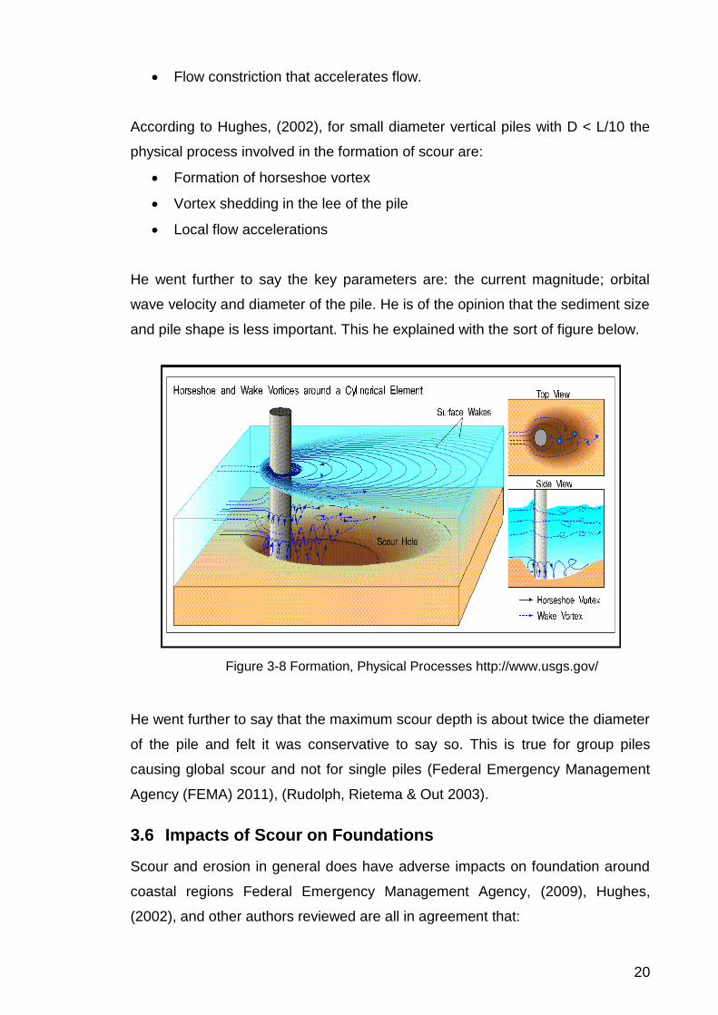
According to Hughes, (2002), for small diameter vertical piles with D < L/10 the
physical process involved in the formation of scour are:
Formation of horseshoe vortex
Vortex shedding in the lee of the pile
Local flow accelerations
He went further to say the key parameters are: the current magnitude; orbital
wave velocity and diameter of the pile. He is of the opinion that the sediment size
and pile shape is less important. This he explained with the sort of figure below.
Figure 3-8 Formation, Physical Processes http://www.usgs.gov/
He went further to say that the maximum scour depth is about twice the diameter
of the pile and felt it was conservative to say so. This is true for group piles
causing global scour and not for single piles (Federal Emergency Management
Agency (FEMA) 2011), (Rudolph, Rietema & Out 2003).
3.6 Impacts of Scour on Foundations
Scour and erosion in general does have adverse impacts on foundation around
coastal regions Federal Emergency Management Agency, (2009), Hughes,
(2002), and other authors reviewed are all in agreement that:
Page 31
21
Scour formation reduces the depth of foundation embedment and causes
foundation to collapse; deep foundations become more susceptible to
settlement; lateral movement or overturning from lateral loads.
Scour formation increases the unbraced length of piles which stresses the
pile and increases the bending moment. This can cause buckling of the
pile.
Linear scour across a building site may like increase foundation flood
loads or lateral loads.
3-9 Local Scour in a Pile Group without Group Interaction
(Federal Emergency Management Agency, 2009)
3.7 Estimation of Scour Depth
3.7.1 Scour Depth around Piles
There are a lot of mathematical predictions for scour depth around piles and all
other marine structures foundation. According to Rudolph, Rietema & Out,
(2003), despite the fact that scour occurrence is a well known phenomenon, little
has been published of field measurement and practical validations of existing
scour prediction formula especially for combined waves and currents. They
carried out a field analysis in conjunction with the Dutch Ministry of Economic
Page 32
22
Affairs, co-sponsored by the oil and gas industry to verify some of these formulas
stated below. Details of the analysis can be found in their work.
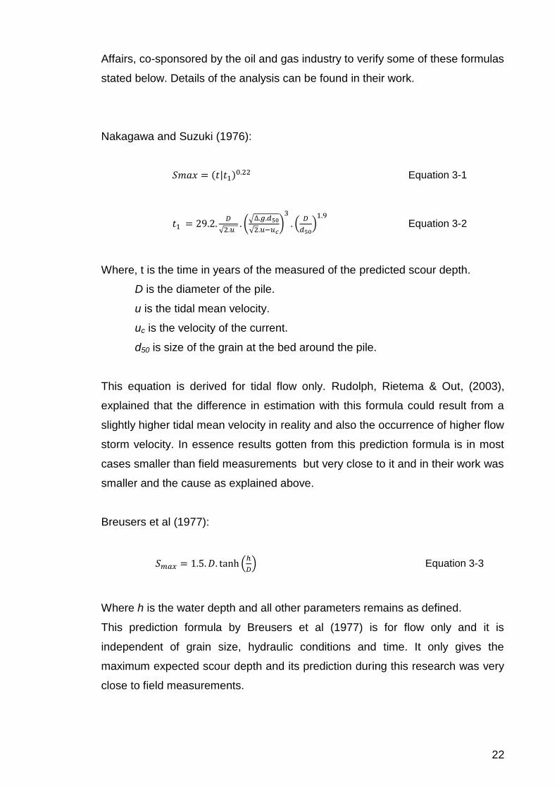
Nakagawa and Suzuki (1976):
Equation 3-1
Equation 3-2
Where, t is the time in years of the measured of the predicted scour depth.
D is the diameter of the pile.
u is the tidal mean velocity.
uc is the velocity of the current.
d50 is size of the grain at the bed around the pile.
This equation is derived for tidal flow only. Rudolph, Rietema & Out, (2003),
explained that the difference in estimation with this formula could result from a
slightly higher tidal mean velocity in reality and also the occurrence of higher flow
storm velocity. In essence results gotten from this prediction formula is in most
cases smaller than field measurements but very close to it and in their work was
smaller and the cause as explained above.
Breusers et al (1977):
Equation 3-3
Where h is the water depth and all other parameters remains as defined.
This prediction formula by Breusers et al (1977) is for flow only and it is
independent of grain size, hydraulic conditions and time. It only gives the
maximum expected scour depth and its prediction during this research was very
close to field measurements.
Page 33
23
Sumer and Fredsoe (2002):
Equation 3-4
With A = 0.03 + 0.75. , KC =
, B = 6. ,
Equation 3.7-4 is an equation that account for waves and currents for the
estimation of scour depth around cylindrical piles. It is only valid for 4 < KC < 25.
According to the researchers the values computed from this formula was rather
very conservative as it under estimates the scour depth. What was clear from
this verification exercise was the fact that the scour formation was still in
progress and the maximum expected scour depth was less than 2 times the
diameter of the pile.
They also researched on pile groups that were jacketed for interaction and found
out that the three formulas prediction where short by a factor of 3-4 times the
piles diameter when compared to field measurements. This was also true in the
Federal Emergency Management Agency, (2009), that most of the piles in group
were found to have suffered from scour exceeding twice the diameters of the
piles. However, Rudolph, Rietema & Out, (2003), did explain that the difference
was as result of the disturbing effect of the jacket structure close to the sea bed.
Another conclusion reached in their research was that of the diameter of the
scour; which was in orders of 30-40 times the diameter of the pile.
Hughes, (2002), also posited that the scour depth can be predicted by the
formula below.
Equation 3-5
Where Sm is maximum scour depth below average bed level
h is water depth upstream of pile
b is pile width
Fr is flow Froud’s number
K1 is pile shape factor
K2 is pile orientation factor
Page 34
24
Hughes, (2002), also believes that there are no analytical method for scour at
vertical piles caused by waves and current. Perhaps, is research was before
Sumer and Fredsoe in 2002. He concluded by saying it is important to note the
dominant scour mechanism for any scour analysis or design.
3.7.2 Scour Depth around Abutments
Most common abutment scour depth prediction formula where developed with
flume test result using cohesionless soils but are used in predicting abutment
scour depth in cohesive soils. Consequently, a rather conservative prediction,
results. In order to produce a cost effective prediction formula for abutment scour
depth in cohesive soils, Seung, Briaud & Chen, (2010) remodified their previous
research results to produce a modified result still known as SCRISCO-EFA
method. They carried several flume tests using porcelain clay and based on the
results and dimension analysis proposed a more cost effective prediction
formula. Also, in their works was the following works mentioned.
3.7.2.1 Froehlich Study
He proposed both clear water and live bed abutment scour prediction formula
using research results of rectangular channels from other researchers
between1953-1985. He made use of 170 live-bed abutment and 164 clear water
abutment scour measurements and by performing data regression, he proposed
the following:
3.7.2.1.1 Clear water scour:
Equation 3-6
3.7.2.1.2 Live bed scour:
Equation 3-7
Page 35
25
Where
is geometric standard deviation for the bed material and D16,
D50 and D84 are particle sizes for the 16th, 50th and 84th percentile by weight of
particle size respectively. , is Froude number base on approach
water depth and the approach water velocity. K1 is correction factor for abutment
shape with values of 1.0, 0.82 and 0.55 for vertical wall, wing wall and spill
through abutment. K2 is the correction factor for the abutments alignment with
respect to the direction of flow with θ being the angle of
abutments alignment – if θ<900 the abutment is skewed downstream and when
θ>900 it is skewed upstream; L’ is the abutments average length
where Ae is the flow area obstructed by the embankment. Y1 is the depth of the
water in the approach section and ys(Abut) is the maximum scour depth.
3.7.2.1.3 Sturm’s Study:
In 2004, Sturm conducted a series of flume test and analysed the results. The
test was carried out on abutment scour depths from compound channels. After
his analysis he suggested the prediction formula below for the maximum scour
depth.
Equation 3-8
Where and M is discharge contraction ratio; Q is the total
discharge and Qblock the block discharge by the approach embankment; qf1 is the
unit flow rate with effect of back water by abutment at the approach section,
( ); qc0 is the critical unit flow rate in the flood plain without the effect
of backwater, ( ), Vf1 is the approach average velocity of the flood
plain and Vfc0 is the critical velocity of the flood plain without backwater effect
; Gs is the specific gravity of the cohesionless
soil, kn is the constant in Strickler-type relationship for Manning’s n (
),
is the critical value of Shield’s parameter, yf0 is water depth on flood plain
without any backwater effect and the approach water depth on the flood plain is
yf1.
Page 36
26
3.7.3 Failures Caused by Scour
Figure 3-10 Abutment Failure Caused by Scour
The figure (9) Fayazi & Farghadan, (2012) above is an abutment failure caused
by scour evident by the depression. It was reported the failure was due to poor
hydraulic design and lack of maintenance of the bridge. The figure (10) Federal
Emergency Management Agency, (2009) below is a differential settlement
caused by scour formation.
Figure 3-11 Differential Settlement Caused by Scour
Page 37
27
3.8 Summary
The chapter in summary has been able to underscore that:
Despite the different ideology in scour concept; scour is a form of water
erosion and it occurs locally around the structure causing obstruction to
flow.
Scour, though a form of erosion is different from general degradation of
the bed of a water course according to FEMA and other researchers.
Scour are of different types usually associated with the bridge structure
e.g. clear water scour; contraction scour; local scour and general scour.
Also, certain conditions must be present for scour formation to occur e.g.
the right current magnitude; the structure; local flow accelerations;
erodible bed etc.
Scour formation reduces embedment depth and causes foundation to
collapse, overturn, increases the stresses on the foundation and other
failures.
There are lots of scour depth prediction formula but are only accurate if
they match the condition e.g. wave only or wave and current or current
only.
It is also mentioned that in the case of piles the equilibrium scour depth
does exceed twice the diameter of the piles even up to four times four
group piles.
Page 38
28
Chapter 4. BUCKLING IN PILES
4.1 Introduction
This chapter gives an overview of pile buckling in engineering. It also talks about
the Euler buckling load and how it is related to piles. The chapter also exposes
the reader to different analytical methods of buckling with reference to piles as
discussed in chapter one (1).
4.2 Buckling
The buckling of slender foundation elements is a common worry for foundation
and structural engineers. As cited by Chance, (2003), many researchers have
addressed the buckling of micro-piles and piles (Bjerrum (1957), Davisson
(1963), Mascardi (1970), Gouvenot (1975)) and their findings came to the
conclusion that only in very loose soil such as sand, peat and clay (with very low
strength properties) that buckling of pile is likely to occur. The Euro code does
support this belief system as well and does treat the buckling of piles rather
conservatively when it stated that buckling should not be checked for piles
embedded in soil with undrained shear strength greater than 10Kpa. However,
the situation for partially free standing piles is becoming more and more
important today because they suffer from buckling. Due to the absence of lateral
support or bracing along its unsupported length, the partially embedded pile is
even of more structural importance than ordinary columns in building when it
comes to buckling. Piles are even more vulnerable to buckling because of
induced eccentricities during installation which is inevitable even under the best
of monitoring and instrumentation conditions (Senthil, Babu, & Pareswaran,
2007). According to Bhattacharya & Bolton, (2004), when structures fail, they
most often result from actions that have been overlooked by designer as
secondary, instead of inadequate factor of safety. The current codes of practice
for pile design such as the Euro code is based on bending mechanism due to
lateral loads. These codes have not considered avoiding the buckling of piles
due to axial loads acting on them caused by diminishing confining pressure
around the pile. He went further to say the current codes have not addressed the
issue of buckling and buckling needs to be addressed for it is the most
destructive form of failure and occurs suddenly.
Page 39
29
4.2.1 Euler Buckling Load
The static axial load for which a frame supported on vertical columns becomes
laterally unstable is known as the ‘Elastic Critical Load’ of the frame commonly
known as ‘Buckling Load’ (Bhattacharya & Bolton, 2004). Buckling load for piles
refers to the allowable compression load for a given unsupported length. During
the 18th century Leonhard Euler the mathematician solved the problem of the
critical compression load of the unsupported length of a column with the basic
equation below (Chance, 2003).
Equation 4-1
Where K is an end condition
I is moment of inertia
E is modulus of elasticity
Lu is unsupported length
For an eccentrically loaded member, the buckling load will be smaller than the
Euler load irrespective of the magnitude of the eccentricity (Senthil, Babu, &
Pareswaran, 2007). To account for the eccentricity a reduction factor is
introduced into the formula.
Equation 4-2
Where α is the reduction factor.
The elastic critical load of a pile can be estimated base on the effective length of
the Euler buckling load for an equivalent pin ended strut. The figure below is
adopted from the column stability theory and it shows the concept of the effective
length theory to normalise the different boundary conditions for pile tip and head.
The simplest way to compute the buckling load of a piled building is to estimate
the buckling load of one pile and multiply it by the total number of piles in the
building. It is of note to point out here that the buckling of piles is different from
normal column buckling available in many literatures; this is because for pile
Page 40
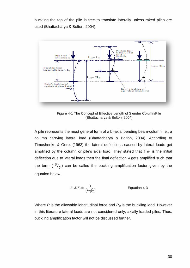
30
buckling the top of the pile is free to translate laterally unless raked piles are
used (Bhattacharya & Bolton, 2004).
Figure 4-1 The Concept of Effective Length of Slender Column/Pile (Bhattacharya & Bolton, 2004)
A pile represents the most general form of a bi-axial bending beam-column i.e., a
column carrying lateral load (Bhattacharya & Bolton, 2004). According to
Timoshenko & Gere, (1963) the lateral deflections caused by lateral loads get
amplified by the column or pile’s axial load. They stated that if is the initial
deflection due to lateral loads then the final deflection gets amplified such that
the term ( ) can be called the buckling amplification factor given by the
equation below.
Equation 4-3
Where P is the allowable longitudinal force and Pcr is the buckling load. However
in this literature lateral loads are not considered only, axially loaded piles. Thus,
buckling amplification factor will not be discussed further.
Page 41
31
4.3 Buckling Analysis of Piles
There are various solutions or methods of analysis that are used for the analysis
of piles for buckling. A few are reviewed below.
4.3.1 Davisson’s Method
Engineering have developed various solutions for determining the buckling load
of piles and one of such solutions is the Davisson’s method. According to
Chance, (2003), in 1963, Davisson described solutions for various boundary
conditions of pile head and tip. He assumed the axial load to be constant
throughout the pile and that there is no load transfer via skin friction. The solution
he proposed is determined from a dimensionless graph of Ucr against Imax. Imax is
computed and Ucr is checked on the graph and substituted into the equation
below to compute the critical buckling load.
Equation 4-4
Equation 4-5
Equation 4-6
Where, is critical buckling load
is modulus of elasticity of the pile shaft
is moment of inertia of pile shaft
is modulus of sub-grade reaction
is a dimensionless ratio
is foundation shaft diameter
L is pile shaft length over which is taken as constant
From figure below it is evident that the boundary condition is of significance and
for a free unrestrained ended pile, the buckling load is the smallest. Table ...
provides the modulus of sub-grade reaction for different soils.
Page 42
32
Figure 4-2 Poulos and Davis 1980 as cited by (Chance, 2003)
Note: The chart above was presented by Poulos and Davis 1980. It is used for
determining the dimensionless Ucr after computing Imax.
4.3.2 Davisson’s and Robinsons Approach
The Davisson and Robinson’s method is an approach that is accepted by
ASSTHO and ACI. The approach was published in 1965 and the correctness of
the approach is in the determination of the equivalent length which is the
unsupported length plus the depth of fixity (Senthil, Babu & Pareswaran 2007).
The depth of fixity is determined by two formulas one for clay and the other for
sand (Arizona Department of Transportation (ADOT) 2010).
Clay
Equation 4-7
Sand
Equation 4-8
Page 43
33
Where is depth of fixity; is elastic modulus of pile; is the moment of
inertia about the weakest axis; is modulus of elasticity of soil in
Ksi and is rate of change of soil modulus with depth.
The equivalent is given by, ( ), where is the unsupported length
of the pile. It is inputted in the Euler buckling formula for an eccentrically loaded
structure.
Equation 4-2
4.3.3 Finite Difference Method
One of the generally accepted ways to analyse piles in soil is to model after the
classical Winkler concept of a beam-column on an elastic foundation. According
to Chance, (2003) the finite difference approach can then be adopted to solve
the resulting differential equation for successive greater loads until a failure to
converge to a solution occurs which is at near the buckling load. The derivation
for the differential equation for beam-columns on elastic foundation was given by
Hetenyi in 1946. According to Chance, (2003), he made the assumption that the
shaft on an elastic foundation is not only subjected to lateral loads but also to
compressive forces acting at the centre of gravity of the end cross section of the
shaft.
Equation 4-9
Where y is lateral deflection of the shaft at point x
x is the distance along the shaft
Q is the axial compressive load on the pile foundation
EI is flexural rigidity of the foundation shaft
Esy is soil rigidity per unit length
Es is secant modulus
Also, in Chance, (2003), the first term of the equation is referred to as equation
of beam subjected to transverse loading and the second term corresponds to the
axial load in the pile shaft. The third term is a mathematical representation of the
Page 44
34
reaction of the soil. Reese & Van Impe, (2001), said that the finite difference
differential equation is adopted to achieve compatibility between pile
displacement and load transfer along a pile shaft and also between the
displacement and resistance at the tip of the pile. However, they did mention that
close agreement has been found for piles in clay with experimental evidence
matching finite difference result citing Coyle and Reese, (1966) and whereas the
results are a bit scattered when it comes to piles in sand citing Coyle &
Sulaiman, (1967). This they tried to explain by saying the effect of the driving of
pile into soil is more severe in sand than in clays in terms of load transfer
characteristics however, the finite difference method can be employed to deal
with any complex composition of soil layers with any nonlinear relationship of
shear versus displacement and can tolerate improvement in the soil criteria
without any alteration to the basic theory.
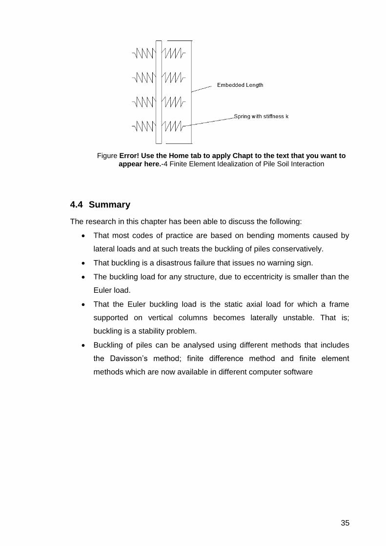
4.3.4 Finite Element Method
According to Sriram, (2001) the normal approach for estimating or computing the
critical load (Buckling load) of a beam column involves finding the root of the
polynomial defined by the determinant below.
Equation 4-10
Where is linear elastic stiffness matrix and
is geometric stiffness matrix
He also said the above equation can be modified by approximating the soil
medium to an elastic medium of stiffness and adding it to the equation as
below.
Equation 4-11
The term in the bracket is the total stiffness of a beam on an elastic foundation.
Page 45
35
Figure Error! Use the Home tab to apply Chapt to the text that you want to appear here.-4 Finite Element Idealization of Pile Soil Interaction
4.4 Summary
The research in this chapter has been able to discuss the following:
That most codes of practice are based on bending moments caused by
lateral loads and at such treats the buckling of piles conservatively.
That buckling is a disastrous failure that issues no warning sign.
The buckling load for any structure, due to eccentricity is smaller than the
Euler load.
That the Euler buckling load is the static axial load for which a frame
supported on vertical columns becomes laterally unstable. That is;
buckling is a stability problem.
Buckling of piles can be analysed using different methods that includes
the Davisson’s method; finite difference method and finite element
methods which are now available in different computer software
Page 46
36
Chapter 5. SOIL-STRUCTURE INTERACTION
5.1 Introduction
The chapter defines and describes briefly soil structure interaction; explaining
what it is and also tells the importance. In order to carry out a proper buckling
analysis as discussed in chapter four (4) and considering scour in chapter three
(3), a proper knowledge of the soil-pile interaction model to be used is
necessary. The literature in this chapter talks about the major ways available for
modelling the interaction between a structure and the soil in which it is planted.
5.2 Definition
Soil structure interaction is the process in which the reaction of the soil
influences the motion of the structure and the motion of the structure also
influences the reaction of the soil; neither the structural or ground displacement
are independent of each other (Hallak, 2012). According to BSi, (2007) it is the
mutual influence of deformation between a foundation or retaining structure and
the soil. According to Dutta & Roy, (2002), there is always an interdependence of
the components of a structure supported by more than one component. They
illustrated this statement with the figure below. They posited that at the central
support, soil below it settle the most due to higher concentration of load over it.
However, the framing action as a result of the beam connecting all three columns
will cause a load transfer to the end columns as soon as the central column
tends to settle more. Thus the forces acting and the final settlement can only be
obtained by considering this interaction, hence, the need for soil-structure
interaction otherwise known as SSI.
There are various approaches to the modelling of Soil-Structure interaction and
one has to be careful, as soil is a very complex material which is heterogeneous,
anisotropic and non-linear in force-displacement characteristics. According to
Chaudhry, (1994), a careful choice of the value of soil shear modulus needs to
be taken to get a reasonable result in soil-structure interaction. There are
basically two classical mathematical models revealed by the search for a closely
realistic physical and mathematical model of the soil media; in soil-structure
interaction analysis; the Winklerian and Continuum model (Dutta & Roy, 2002).
Page 47
37
5.2.1 Winkler Model
This method of modelling the soil structure interaction is still been employed
greatly by civil engineers and researchers. In his literature Bezgin, (2010), said
that the Winklers’s hypothesis is an approximation of the soil reaction to a
distributed loading taking into account the soil stiffness. Some other researchers
and engineers say that it is an approximation of the soil medium by closely
spaced independent elastic springs Murthy, (2002) and Dutta & Roy, (2002).
Which is all one and same thing, since the stiffness of the spring represent the
stiffness of the soil. According to Dutta & Roy, (2002), the deformation in this
idealization is confined to loaded region only. The Winkler model is based on a
beam on elastic foundation Dutta & Roy, (2002), Bezgin, (2010) and (Murthy
2002). The inter soil-layer coupling which is the transfer of shear between soil
layers parallel to the direction of loading is disregarded by Winkler’s hypothesis
and this is the fundamental medium by which load is borne and transferred by
the soil layers. Any mathematical model lacking this has got a disadvantage
inbuilt (Bezgin, 2010). Also, Dutta & Roy, (2002) sees a problem with this model
which is inherent in determining the stiffness of the elastic springs with which to
replace the soil of the foundation. He says the problem is two folds since the
numerical value of the coefficient of sub-grade reaction do not only depend on
the nature of the sub-grade but also on the dimension of the loaded area.
Figure 5-1 Soil Structure-Interaction
Page 48
38
However, Murthy, (2002), citing Vesic, (1961) says the errors inherent in the
Winkler’s model is not significant.
Figure 5-2 Winkler's Beam on Elastic Foundation
5.2.1.1 Application to deep foundation
The logic and theories from research discoveries on slabs or beam-columns
resting on soils can be applied to any foundation including piles (Bezgin, 2010).
For a soil supported beam-column under axial and transverse load, the beam
sub-grade reaction (contact stress) variation along the structural element is not
necessarily zero and will be continuous in most cases. The differential equation
of a beam column under axial and transverse loading resting on a soil is
expressed below.
Equation 5-1
Where EI is the beams flexural stiffness
P is the axial load
is the sub-grade reaction
is the transverse loading
Figure 5-3, Axial and Transversely Loaded Beam-Column on Soil
Page 49
39
Alternatively, the interaction between the beam or beam column and the soil
under axial and transverse loading can be written in matrix stiffness formulation
as below.
Equation 5-2
Equation 5-3
Where S is the flexural stiffness matrix for the beam-column
is the displacement vector
is the sub-grade reaction vector
is the load force vector
is the stiffness of the soil with respect to the width of the beam
What is important at this point according to (Bezgin, 2010), is to describe p(x) or
in a parametrically compatible format with the rest of the term in the equation.
This is the strongest attraction of the Winkler’s hypothesis is that all of the effects
of the sub-grade reaction can be expressed as the displacement, .
Automatically, is removed from the equation above and it becomes modified
and like that of a beam or beam-column on elastic foundation as shown below.
This very simplicity is the very reason why the Winkler’s hypothesis is widely
used in the field of engineering.
Equation 5-4
Equation 5-5
is the modified flexural stiffness matrix to include the reaction of the soil.
5.2.1.2 Modelling the Spring Stiffness
In the Winkler type model, an important parameter in the modelling of the soil
spring is the subgrade reaction. Terzaghi, (1955), subgrade reaction of slab or
beam is the pressure ‘p’ per unit area of the contact surface between the slab or
beam and the subgrade in which it is planted. The subgrade reaction at any
Page 50
40
distance ‘x’ from the midpoint of the length of a loaded plate or beam is given by
the expression below.
Equation 5-6
Where ‘y’ is the deflection of the plate at that point and is the coefficient of
subgrade reaction. The coefficient of subgrade reaction is the ratio of the
pressure at the contact surface between a slab or beam and the subgrade to the
consequent displacement ‘y’ Terzaghi, (1955) and Briaud, (2001). The unit is
force per unit volume Bezgin, (2010), Briaud, (2001) and Terzaghi, (1955).
Critically looking at the unit of the slope in the graph below a better idea of this
parameter can be easily conceptualise as the unit can be deceptive without
critically looking at the parameter.
Figure 5-4 A Graph of Coefficient of Subgrade Reaction
From the figure above the unit is force per unit area per displacement for
coefficient or modulus of subgrade reaction (Bezgin 2010). There is another bit
of confusion that arises when the term coefficient or modulus of subgrade
reaction is referred to as spring constant as seen in many literatures Pavement
Interactive (2007), Monaco & Marchetti, (2004) as the units are not the same.
Spring constant from Hooke’s law is force per unit length contrary to coefficient
of subgrade reaction force per unit area per length. A simple explanation to this
is to say; the coefficient of subgrade reaction is the coefficient of the spring
constant (in a Winkler’s type model) around the loaded area such that multiplying
Page 51
41
the coefficient of subgrade reaction at a point in the loaded area by the
magnitude of the loaded area gives the spring stiffness at that point in (F/L).
Equation 5-7
Where is the spring stiffness as defined by ‘Hooke’s Law’; , is coefficient of
subgrade reaction and is the loaded area.
5.2.1.2.1 Vertical Subgrade reaction
The method of determining the subgrade reaction for beams and slabs is by
correlating it to a value from a plate load test. The value of the plate load test is
gotten by averaging the values of several tests on the site of interest. However,
in the absence of a plate load test the reaction can be estimated from the
empirical values in the table below. The danger inherent in this approach is if the
limiting value of the site is lower than the chosen value (Terzaghi 1955).
Table 5-1 Values of ks1 (KN/m3) for 1ft square plate on sand (Terzaghi 1955)
Relative Density of Sand Lose Medium Dense
Dry or moist sand, Limiting values
for
6929-20786 20786-103929 103929-
346429
Dry or moist sand, Proposed values 13857 45036 173214
Submerged sand, Proposed values 8661 27714 103929
The vertical subgrade reaction is given by
Equation 5-8
, and defines the modulus of vertical subgrade reaction and basic value of
the coefficient of vertical subgrade reaction respectively. is determinable
from a plate load test.
For cohesive soils the vertical subgrade reaction can be determined by the
expression below.
Page 52
42
(Terzaghi 1955). Equation 5-9
Table 5-2 Ks1 values (KN/m3) for pre-compressed clay (Terzaghi 1955)
Consistency of Clay Stiff Very Stiff Hard
Values of KN/sq.m 95.76-191.52 191.52-383.04 >383.04
Range for square plate 17321-34643 34643-69286 >69286
Proposed values, square plate 25982 51964 103929*
5.2.1.2.2 Horizontal Subgrade Reaction
The coefficient of horizontal subgrade reaction of a vertical pile or pier
surrounded by sand at a depth ‘z’ below the surface of the sand is a function of
the width ‘D’ of the pile measured at right angles in the direction of the
displacement, the effective unit weight and relative density of the sand. It is
determined by the relationship between the contact pressure ‘p’ and the lateral
displacement ‘y’ due to the deformation of the adjacent soil medium with
modulus Es. The limit of this deformation is 3D beyond which there is no effect
on the local bending moment (Terzaghi 1955).
Equation 5-10
, is a coefficient dependent on the density of the sand and is the effective
overburden pressure and , is the constant of subgrade reaction.
Table 5-3 and values for Sand (Terzaghi 1955)
Relative Density Lose Medium Dense
Ranges of values of 100-300 300-1000 1000-2000
Dry Moist Sand (KN/m3) 2425 7275 19400
Submerged Sand (KN/m3) 1386 4850 11779
Page 53
43
The constant of subgrade reaction is the variation of the modulus of elasticity E
with depth for cohesionless soil. However, E is constant for cohesive soils
(Terzaghi 1955). According to Bezgin, (2010) this variation has been tested by
Prakash, (1962) and found that the variation is non-linear though, a linear
variation is acceptable.
Equation 5-11
The exact value of can only be gotten from field test in which absence
correlations from previous test and research can be used Terzaghi, (1955) and
Bezgin, (2010).
For piles embedded in clay the values of can be assumed to be
approximately same with for beams resting on the horizontal surface of the
same clay. The error in this assumption is on the safe side because the
horizontal deflection of a pile of an assumed with 30cm is smaller than that of a
strip of equivalent width on the same clay and at an equal surface pressure per
unit area (Terzaghi 1955). Below are expressions proposed by different
researchers.
(Terzaghi 1955)
Broms, (1946) as cited by Chin, Sew & Chung, (2009)
Skempton, (1951) as cited by Chin, Sew & Chung, (2009)
, and are the secant modulus and undrained shear strength of the soil
respectively.
5.2.2 Elastic Continuum Model
This is an approach formulated from continuum mechanics to deal with the
boundary condition of soil as is infinite in nature and also continuous in the
distribution of displacement and applied stresses. This model, also known as
‘Elastic Half-Space Model’ and it is said to have three dimensional idealisation
Page 54
44
(Vasani 2003). According to Dutta & Roy, (2002), to make it simple, the soil is
considered isotropic and semi-infinite when modelling and that the effect of soil
layering and anisotropy could be accounted for during the analysis. They also
said that the approach provides more information on the deformation and
stresses within the soil mass and Vasani, (2003), in his work agrees to this when
he said the response function of an elastic half-space/plain is characterized by
the deflected shape of the surface of the elastic medium subjected to a
concentrated stress/force of infinite extent. Both authors agree that this
idealisation is a lot more intricate from a mathematical view point and Dutta &
Roy, (2002) believes, this limits the application of this model severely despite
stating that there is the advantage of simplicity of input parameters over the
Winkler’s model viz the poison’s ratio and modulus of elasticity. One of the major
setbacks of this model is the inaccurate prediction of the reactions around the
peripheries of the foundation and for soil in reality displacement decreases
downward more rapidly than it is predicted by this model (Dutta & Roy, 2002).
5.3 Summary
The chapter in summary is:
Soil structure interaction is the mutual influence of deformation between a
structure and the soil in which it is planted.
There are basically two classical mathematical models that closely model
the soil structure interaction realistically; the Winkler’s and Continuum
model.
Winkler’s model is widely used because results gotten from it are more
realistic and it is also mathematically easier to model.
The major limitation of the Winkler’s model is that it does not consider the
soil as a continuum and the transmissibility of load through inter-soil layer
coupling is also ignored.
The coefficient of subgrade reaction is the coefficient of the spring
stiffness (in a Winkler type model) of any point in the loaded area.
Page 55
45
Chapter 6. RESEARCH METHOD
6.1 Overview
This is the methods chapter; it is a product of the literatures read of which many
where reviewed in chapters; 2, 3, 4 and 5. This chapter describes the samples,
mathematical model and software used in this research. It gives a description of
the pile sample; sample scour depth for both single and group piles; sample soil
stiffness; the mathematical model, the software used and a brief description of
the procedure used in combining these samples via mathematical model and
software to achieve the aim of this research.
6.2 Sample Description
6.2.1 Pile:
The sample pile is a pile 20m in length and embedded 10m into the underlying
ground. It has a free unsupported 10m length above the ground surface and
diameter 0.30m, 0.4m, 0.5m, 0.6m and 0.7m. The elastic modulus of the steel
material is 205GPa. This description is for both single and group piles. There are
actually no criteria for choosing this pile other than the simplification of modelling
when compared to a composite pile and the benefit of not worrying over the non
linear behaviour of the modulus of elasticity of concrete.
6.2.2 Scour Depth:
The sample equilibrium scour depth has been chosen based on extensive
literature review on the subject matter of scour particularly with piles (see
appendix A). This depth has been chosen with limitation to scour caused by pile
actions only either as a single pile or as in a group of piles and does not include
any global scour that may result from any other structural interference except
those caused by the group’s action in the water course. The sample scour depth
has been chosen to vary from a depth of zero times the diameter (0D) to twice
the diameter (2D) for single piles and from zero times the diameter (0D) to six
times the diameter (8D) for group piles affected by group action.
6.2.3 Soil Stiffness:
The sample soil is sandy and its stiffness was adapted from the expressions of
Terzaghi, (1955) and Khazanovich as cited by Ping & Sheng, (2011). A value of
Page 56
46
was picked from Table 5-3 and values for Sand and using the
expression below was determined for various depth z below the surface of the
sand.
Equation 5-10
Where D is the pile width B and is the rate of change of soil modulus. , is
the modulus of subgrade reaction.
Equation 6-1
Where ‘ ’ is the equivalent spring stiffness for the soil and ‘ ’ is half the surface
area of the pile.
To model the pile-soil interaction of the representative piles in the group model
correctly; the modulus ( ) deterioration is considered according to Arizona
Department of Transportation (ADOT), (2010) citing Prakash, (1990), who found
that for spacing between piles greater than 8 times the diameter of the piles,
neighbouring piles have no effect on the soil modulus or buckling resistance.
However, at a spacing 3 times the diameter, the soil modulus is reduced by 25%.
For other spacing the value of the soil modulus can be interpolated. In this
research 50% deterioration is considered thus the table below.
Table 6-1 Adopted Values for nh from Terzaghi 1965
Relative Density Lose Medium Dense
Single Pile Sand (KN/m3) 1000 3000 9000
Group Pile Sand (KN/m3) 500 1500 4500
6.2.4 Mathematical Model:
The Winkler’s model has been adopted for this thesis over the continuum
mathematical model and the very reasons as stated in the literature review under
chapter five (5). Also, in order to solve the Winkler’s model, FEM method has
been chosen over analytical approach. The FEM method is chosen over
analytical methods because FEM method with the aid of computer software
Page 57
47
saves a lot time which is not available for an analytical approach to the problem.
Also, the FEM models will yield more accurate results as the model is not treated
as a unit as in analytical methods but as little individual elements whose
individual response is summed up together to give the FEM result.
6.2.5 Software:
StaadPro finite element software is the software of choice because of its
popularity in the modelling industry and availability for the purpose of academic
work under a special license agreement from the University of East London. It
can be used to do several analysis ranging from linear to non-linear; p-delta and
including buckling which is estimated by computing the buckling factor. The
buckling factor is a factor by which the applied load is multiplied to get the
buckling load. One of the major reasons for choosing this software is that of level
of accuracy, though no other software was tested; this is able to estimate the
buckling capacity with an error less than 0.3 % - 4% as shown in the verification.
6.3 Procedure:
The procedure involves modelling the geometry of the sample pile in Staad
software using staad space. Staad space is used because buckling is analysed
on the weakest axis of a structure and at such the software is able to check all
three axis as against plane and give a correct response. The geometry is broken
into forty (40) elements using the insert node function. Twelve elements is the
number of elements beyond which the buckling factor calculated by Staad does
not change significantly for the unsupported sample pile. In addition to the
existing elements; twenty more elements are created of the twenty elements in
the embedded half of the pile. This is necessary to model the pile soil interaction
correctly with little error by using nodes that are closely spaced so that no
change is caused when splitting up elements further by inserting nodes to model
the investigated scour depth correctly. Nodes are inserted at the very points
where the springs representing the soil stiffness are attached. The steel material
and circular geometry is modelled in the ‘Section Property’ tab and applied to all
elements. The spring stiffness is inserted for Kx and Kz in the ‘Fixed But’ tab and
inserted into the appropriate nodes. The Pile head is modelled using springs as
Page 58
48
well but of very high stiffness. The applied load of which the buckling factor is
calculated for this research has been chosen to be 100KN. In the analysis print
tab, buckling analysis is selected but with a minimum of 30 iterations which is the
number of iterations required to give a stable result for the largest pile model.
Page 59
49
Chapter 7. VERIFICATION
7.1 Overview
This chapter verifies the generated FEM models and the utilised corresponding
boundary conditions representing the pile cap and the soil medium against two
special cases of which analytical results are available. The model is verified
against the Euler buckling load theory see chapter 4 page (29) and the modified
Euler load theory of piles in clay by Davisson’s (Chance 2003). Also, this chapter
sets the limit as to the accuracy of the Results chapter (chapter 8) and at the end
would have verified chapter six (6), the methods chapter.
7.2 Euler Buckling Load Theory
Equation 4-1
Where K is an end condition
I is moment of inertia
E is modulus of elasticity
Lu is unsupported length
7.2.1 Fixed-Pin Ended Boundary
Figure 7-1 A Fixed-Pin Ended Boundary Condition (Arizona State University 2003)
Page 60
50
For a fixed-pin ended column K is 0.7 and solving that for a column (equivalent
of a pile with no soil support) with the following geometrical characteristics,
diameter 0.15m and length 12m with modulus of elasticity of 205GPa gives
713.99KN. The finite element model produced a value of 713.75KN when divided
into ten elements and changed no further even with more elements.
Figure 7-2 3-D Model Showing Pile Section
Figure 7-3 Finite Element Model for a Fixed-Pin Ended Condition
Page 61
51
7.2.2 Fixed-Fixed Ended Boundary
Figure 7-4 Fixed-Fixed Boundary Condition (Arizona State University 2003)
For a fixed-fixed boundary condition K=0.5 and for a pile with the same geometry
as above the critical buckling load of the column is 1399.43KN and the finite
element model produced a buckling strength of 1395.00KN
Figure 7-5 FE Model for a Fixed-Fixed Boundary Condition
Page 62
52
7.2.3 Pinned-Pinned Boundary Condition
Figure 7-6 Pinned-Pinned Boundary Condition (Arizona State University 2003)
For the same column but with a pinned-pinned boundary condition K=1 and the
Euler buckling load is 349.86KN and the finite element model yielded 349.06KN.
Figure 7-7 FE Model for Pinned-Pinned Boundary Condition
Page 63
53
7.2.4 Variation of Pcr with FE Elements
Below is a table showing the variation of the critical buckling load with variation in
the number of elements used in the FE models for the column above.
Table 7-1 Variation of Pcr with No: of FE Elements
No of Elements
Fixed-Pin (KN)
Fixed-Fixed (KN)
Pin-Pin (KN)
1 1060.63 inconclusive 424.38
5 714.38 1398.75 349.06
10 713.75 1395.00 349.06
20 713.99 1395.00 349.06
7.3 Davisson’s Method
The Davisson’s method for piles in clay produced a theoretical value of 32.69kips
(32,690Ib, 145.41KN) for a pin-pin ended condition which is said to be very
conservative (Chance 2003). A value close to this was achieved in the finite
element model by inputting the stiffness in the x-z direction for three (3) nodes
(33,575Ib) and for nine (9) nodes (148,000Ib). This proves as well that the
Davisson’s method is very conservative in estimating the buckling capacity of
beams in elastic foundation.
Where, is critical buckling load
is modulus of elasticity of the pile shaft
is moment of inertia of pile shaft
is modulus of sub-grade reaction
is a dimensionless ratio
is foundation shaft diameter
L is pile shaft length over which is taken as constant
Page 64
54
Table 7-2 Pile Properties
d Ip Ep
1.5 inch 0.396 inch4 30x10
6psi
0.0381 m 2.107x10⁻⁶
m4 206842719 KN/m
2
From figure 4-2
Figure 7-8 The Finite Element Model
Table 7-3 Variation of Pcr with No: of Nodes having Spring Stiffness
Nodes Pcr(Ib) Pcr(KN)
3 33,575.00 149.35 4 69,000.00 306.93 9 148,000.00 658.34 18 205,800.00 915.44
The table above shows that the more nodes created having spring stiffness
equivalent to that of the soil at that level the higher the buckling capacity of the
Page 65
55
pile. The closer the nodes are to one another the more accurate the result is to
modelling the soil stiffness.
7.4 Variation of Pcr for Different Pile Head Boundary Condition
Table 7-4 below shows that lateral and rotational stiffnesses can be effectively
used to model the different known pile head boundary condition successfully.
Table 7-4
Pile Head Boundary
Condition
Pcr (KN) Pile Head stiffness
(KN/m; KN-m/Ɵ)
Pcr (KN)
Fixed 23,255.00 (728,000;70,000) 23,137.50
Pinned 11,893.75 (728,000;0) 11,893.75
Free 1,463.20 (0;0) 1,463.20
7.5 Conclusion
The above two verification proves that the model can be used. The first
verification shows that the model can be used in estimating the buckling capacity
of a column (the equivalent of a pile with no soil support). The second verification
shows that the finite element software (StaadPro) can be used to model a beam
in a Winkler’s type foundation successfully. Also, it shows that the level of
accuracy depends on the number of nodes created and the number springs
introduced to these nodes. The more the nodes created having spring stiffness
representing soil stiffnesses at the level of the nodes the more accurate the
model is to the soil as a continuum and not a series of individual springs in the
pile-soil-interaction. The last verification shows that the various pile heads can be
modelled by inputting equivalent spring stiffnesses in the model.
Page 66
56
Chapter 8. RESULTS
8.1 Overview
This chapter presents the important results of the research which this thesis has
carried out and verified in chapter 7. It is important to remind the reader what this
thesis is all about again. This research is to show how scouring around piles
affect the tendency of the piles to buckle by looking at two categories of piles.
Piles with enough spacing to be regarded as monopiles or monopiles or piles
affected by the group effect (Soil stiffness/modulus deterioration and global scour
effects). It is important to recall the research questions to be able to appreciate
the results.
1. How does the buckling capacity of a partially free standing pile vary with
scour depth?
2. How does Pile Group action affect the buckling capacity of a scoured
partially free standing pile?
3. To what extent does the soil condition affect the buckling capacity of a
scoured partially free standing pile?
4. What is the response of a scoured partially free standing pile buckling
capacity to different pile head stiffnesses assuming full fixity of pile tip?
See Appendix A for results on normalised scour depth gotten from literature
review and below is a figure of the finite element model.
Figure 8-1 Figure of the Finite Element Model
Page 67
57
8.2 Variation of Buckling Strength with Normalised Scour Depth
8.2.1 Monopiles
These results are presented first of other results because they help the reader to
see how scouring affects the buckling strength of a partially free standing pile
under scoured condition. The normalized scour depth is the ratio of the scour
depth to the pile diameter ‘B’.
In figure 8-1 to 8-3 it can be seen clearly that the relationship between Pcr and
the normarlised scour depth is an inverse relationship. The buckling strength
decreased with increasing normalised scour depth. The relationship appears to
be linear for all diameters. These graphs also show that buckling strength
increases with pile diameter.
Figure 8-2
0.00 20,000.00 40,000.00 60,000.00 80,000.00
100,000.00 120,000.00 140,000.00 160,000.00 180,000.00 200,000.00 220,000.00 240,000.00 260,000.00 280,000.00 300,000.00 320,000.00 340,000.00 360,000.00 380,000.00 400,000.00 420,000.00 440,000.00 460,000.00 480,000.00 500,000.00
0 0.5 1 1.5 2 2.5
Pc
r (K
N)
Normalised Scour Depth (S/B)
Pcr Vs Normalised Scour Depth nh1(Loose Sand) Soil Monopiles
Pcr30cm
Pcr40cm
Pcr50cm
Pcr60cm
Pcr70cm
Page 68
58
Figure 8-3
Figure 8-4
0.00 20,000.00 40,000.00 60,000.00 80,000.00
100,000.00 120,000.00 140,000.00 160,000.00 180,000.00 200,000.00 220,000.00 240,000.00 260,000.00 280,000.00 300,000.00 320,000.00 340,000.00 360,000.00 380,000.00 400,000.00 420,000.00 440,000.00 460,000.00 480,000.00 500,000.00 520,000.00 540,000.00 560,000.00
0 0.5 1 1.5 2 2.5
Pc
r (K
N)
Normalised Scour Depth (S/B)
Pcr Vs Normalised Scour Depth nh2(Medium Sand) Soil Monopiles
Pcr30cm
Pcr40cm
Pcr50cm
Pcr60cm
Pcr70cm
0.00 20,000.00 40,000.00 60,000.00 80,000.00
100,000.00 120,000.00 140,000.00 160,000.00 180,000.00 200,000.00 220,000.00 240,000.00 260,000.00 280,000.00 300,000.00 320,000.00 340,000.00 360,000.00 380,000.00 400,000.00 420,000.00 440,000.00 460,000.00 480,000.00 500,000.00 520,000.00 540,000.00 560,000.00 580,000.00 600,000.00
0 0.5 1 1.5 2 2.5
Pc
r (K
N)
Normalised Scour Depth (S/B)
Pcr Vs Normalised Scour Depth nh3(Dense Sand) Soil Monopiles
Pcr30cm
Pcr40cm
Pcr50cm
Pcr60cm
Pcr70cm
Page 69
59
8.2.2 Group Piles
The graphs in this section 8.2.2 show similar trends. There is an inverse
relationship between Pcr and the normalised scour depth. The relationship is
linear for all pile diameters. The buckling strength increases with pile diameter.
Figure 8-5
Figure 8-6
0.00 20,000.00 40,000.00 60,000.00 80,000.00
100,000.00 120,000.00 140,000.00 160,000.00 180,000.00 200,000.00 220,000.00 240,000.00 260,000.00 280,000.00 300,000.00 320,000.00 340,000.00 360,000.00 380,000.00 400,000.00 420,000.00 440,000.00 460,000.00 480,000.00
0 2 4 6 8 10
Pc
r (K
N)
Normalised Scour Depth (S/B)
Pcr Vs Normalised Scour Depth nh1(Loose Sand) Soil Group Piles
Pcr30cm
Pcr40cm
Pcr50cm
Pcr60cm
Pcr70cm
0.00 20,000.00 40,000.00 60,000.00 80,000.00
100,000.00 120,000.00 140,000.00 160,000.00 180,000.00 200,000.00 220,000.00 240,000.00 260,000.00 280,000.00 300,000.00 320,000.00 340,000.00 360,000.00 380,000.00 400,000.00 420,000.00 440,000.00 460,000.00 480,000.00 500,000.00 520,000.00
0 2 4 6 8 10
Pc
r (K
N)
Normalised Scour Depth (S/B)
Pcr Vs Normalised Scour Depth nh2(Medium Sand) Soil Group Piles
Pcr30cm
Pcr40cm
Pcr50cm
Pcr60cm
Pcr70cm
Page 70
60
Figure 8-7
8.3 Variation of Pcr with Normalised Scour Depth for Different
Soil Condition for 30cm pile
The results presented in this section show the relationship between the critical
buckling load and the normalised scour depth for different soil densities. Also,
the 30cm diameter pile has been chosen as the sample pile for this section both
for monopiles and group-piles also soil stiffness increases from nh1 to nh3.
8.3.1 Monopile
As seen in the graph below Pcr varies inversely with normalised scour depth and
the relationship is linear. It is also observed in the graph that the buckling
strength increases with increasing soil density. There is an increase of 6.72% of
the buckling strength of the pile from nh1 to nh2 soil, 6.28% from nh2 to nh3 and
13% of the buckling strength from nh1 soil to nh3 along any path of the curve.
0.00 20,000.00 40,000.00 60,000.00 80,000.00
100,000.00 120,000.00 140,000.00 160,000.00 180,000.00 200,000.00 220,000.00 240,000.00 260,000.00 280,000.00 300,000.00 320,000.00 340,000.00 360,000.00 380,000.00 400,000.00 420,000.00 440,000.00 460,000.00 480,000.00 500,000.00 520,000.00 540,000.00 560,000.00 580,000.00
0 2 4 6 8 10
Pc
r (K
N)
Normalised Scour Depth (S/B)
Pcr Vs Normalised Scour Depth nh3(Dense Sand) Soil Group Piles
Pcr30cm
Pcr40cm
Pcr50cm
Pcr60cm
Pcr70cm
Page 71
61
Figure 8-8
8.3.2 Group Piles
The trend in graph presented below is the same as the ones in the figure 8-7.
The exception is that beyond 2B which is exactly where the graph in figure 8-7
ended, the relationship between Pcr and the normalised scour depth for the
different soil appears to be closer as the normalised scour depth increase.
Figure 8-9
22,000.00
22,500.00
23,000.00
23,500.00
24,000.00
24,500.00
25,000.00
25,500.00
26,000.00
26,500.00
0 0.5 1 1.5 2 2.5
Pc
r (K
N)
Normalised Scour Depth (S/B)
Variation of Pcr with Scour Depth for Different soil 30cm Diameter Pile
Monopile
nh1(Loose)
nh2(Medium)
nh3(Dense)
0.00 2,500.00 5,000.00 7,500.00
10,000.00 12,500.00 15,000.00 17,500.00 20,000.00 22,500.00 25,000.00 27,500.00
0 2 4 6 8 10
Pc
r (K
N)
Normalised Scour Depth (S/B)
Variation of Pcr with Scour Depth for Different soil 30cm Diameter Pile Group
Pile
nh1
nh2
nh3
Page 72
62
8.4 Variation of Buckling Strength with Pile Head Stiffness and
Normalised Scour Depth
The result illustrated in figure 8-10 shows there is a negligible relationship
between the critical buckling loads of the partially free standing pile and the pile
head stiffness between 0.2 and 1 of the pile head stiffness; there is only a 1.5%
change in Pcr from 1 to 0.2 of the rotational stiffness. The relationship changes
into a linear between 0.2 and 0.0 of the pile head stiffness.
Figure 8-10
Figure 8-11 shows that variation between the horizontal stiffness and the critical
buckling load is linear till a certain point where it becomes approximately
constant. The trend is the same at different scour depth but as the scour depth
reduces the embedment depth the critical buckling load reduces.
0.0
5,000.0
10,000.0
15,000.0
20,000.0
25,000.0
0.00 0.10 0.20 0.30 0.40 0.50 0.60 0.70 0.80 0.90 1.00
Pcr
(K
N)
Rotational Stiffness (KN-m/Ɵ/KN-m/Ɵ)
Pcr Vs Rotational Stiffness Horizontal Stiffness Constant
Page 73
63
Figure 8-11
8.5 Percentage Variation of Buckling Strength at Maximum
Scour Depth for Different Pile Diametres
8.5.1 Monopiles
The results in figure 8-11 to 8-12 show that buckling strength increases with
increase in pile size. There is a larger decrease in buckling strength from the
initial at no scour depth to the buckling strength at maximum scour depth as the
pile size increases for monopiles. The trend in the three soil types (nh1, nh2 and
nh3) examined is the same. The relationship is linear but not perfectly; between
30cm and 50cm pile size the relationship could be said to be linear from the
graphs. However, between 50cm to 70cm pile size the relationship is
inconsistent.
Figure 8-12
0.0
5,000.0
10,000.0
15,000.0
20,000.0
25,000.0
0.00 0.10 0.20 0.30 0.40 0.50 0.60 0.70 0.80 0.90 1.00
Pcr
(K
N)
Horizontal Stiffness (KN/m/KN/m)
Pcr Vs Horizontal Stiffness Rotational Stiffness Constant
Pcr0B
Pcr2B
Pcr4B
Pcr6B
0.00
2.00
4.00
6.00
8.00
30cm 40cm 50cm 60cm 70cm
% D
ec
rea
se
in
Bu
ck
lin
g
Str
en
gth
Pile Diameter
% Variation of Buckling Strength with Pile Diametre nh1 Soils
Page 74
64
Figure 8-13
Figure 8-14
8.5.2 Group Piles
For the group piles at the maximum scour depth the relationship between the
decrease in buckling strength and the pile size is linear for all three soil (nh1, nh2
and nh3) condition. There is an increase in the percentage of decrease in the
buckling strength from zero scour depth to maximum scour depth as the pile size
increases. The decrease is higher for the denser soil; 44% for 70cm pile in dense
sand; 40%for medium and 36% in loose sand.
0.00
2.00
4.00
6.00
8.00
10.00
30cm 40cm 50cm 60cm 70cm
% D
ec
rea
se
in
Bu
ck
lin
g
Str
en
gth
Pile Diameter
% Variation of Buckling Strength with Pile Diametre nh2 Soils
0.00
5.00
10.00
15.00
30cm 40cm 50cm 60cm 70cm
% D
ec
rea
se
in
Bu
ck
lin
g
Str
en
gth
Pile Diameter
% Variation of Buckling Strength with Pile Diametre nh3 Soils
Page 75
65
Figure 8-15
Figure 8-16
Figure 8-17
0.00
10.00
20.00
30.00
40.00
30cm 40cm 50cm 60cm 70cm
% D
ec
rea
se
in
Bu
ck
lin
g
Str
en
gth
Pile Diameter
% Variation of Buckling Strength with Group Pile Diametre nh1 Soils
0.00
10.00
20.00
30.00
40.00
50.00
30cm 40cm 50cm 60cm 70cm
% D
ec
rea
se
in
Bu
ck
lin
g
Str
en
gth
Pile Diameter
% Variation of Buckling Strength with Group Pile Diametre nh2 Soils
0.00
10.00
20.00
30.00
40.00
50.00
30cm 40cm 50cm 60cm 70cm
% D
ec
rea
se
in
Bu
ck
lin
g
Str
en
gth
Pile Diameter
% Variation of Buckling Strength with Group Pile Diametre nh3 Soils
Page 76
66
Chapter 9. DISCUSSION
9.1 Overview
In this chapter the results presented in the previous chapter will be thoroughly
discussed and analysed against previous researches. It will follow exactly the
same heading levels as the previous chapter.
9.2 Variation of Buckling Strength with Normalised Scour Depth
From the results it can be clearly seen that buckling capacity decreases with
increasing normalised scour depth. This is due to the reduction in the confining
pressure due to diminishing depth of embedment, thus there is an increase in the
unsupported length of the partially free standing pile. As seen in Euler’s critical
buckling formula (see section 4.2.1), with all other parameters remaining
constant an increase in ‘L’ will cause Pcr to decrease. Also, this result
corroborates the findings of recent research carried out by Cheng et al. (2010)
that Pcr decreases with increasing scour depth.
Also, it was observed that the relationship between Pcr and the normalised scour
depth are linear for the mono-piles and group piles in all soil condition. When
compared to previous research by Cheng et al. (2010), this is different (see
appendix B). This difference may have arisen from the mathematical model, this
research has adopt a system of mutually independent linear springs Winkler type
whereas, the research by Cheng et al. (2010) used an approximated p-y curve
by Reese et al, (2004) generated by the software L-pile and the values are made
an input in a Multilinear spring model in StaadPro structural analysis software,
there by introducing non-linearities in their model. Also, in this research linearly
increasing soil stiffness with depth is considered whereas a p-y curve is gotten
either from experiment there by capturing non-linearities of the soil or from non-
linear mathematical model that relates soil depth to changes in modulus.
9.3 Variation of Pcr with Normalised Scour Depth for Different
Soil Condition for 30cm pile
Variation of the buckling capacity for different soil condition for the same pile
shared the same trend for different pile diameters. The result showed that
buckling strength increase with increasing soil density nh1>nh2>nh3 i.e. loose,
Page 77
67
medium and dense sand. This is as expected and proves Davisson’s and
Robinsons Approach to pile buckling analysis to be right. Thus, stiffer soil
reduces the depth of fixity of the pile consequently reducing the buckling length
see page 31. The increase is 6.72% of the buckling strength of the pile from nh1
to nh2 soil, 6.28% from nh2 to nh3 and 13% of the buckling strength from nh1
soil to nh3 both for monopiles and group piles. However, at lower normalised
scour depth beyond 2B this difference is neglible. This corroborates findings from
the research of Cheng, et al. (2010) as seen in appendix B. The pile’s buckling
load increased from loose sand to dense sand, however the difference was small
and very minor at shallower scour depth Cheng, et al. (2010). Also, this conforms
to mathematical logic for as the scour depth increases the pile geometry and
material increasingly becomes the element of the buckling strength of the pile-
soil interaction system. At scour depth equals depth of embeddment and
assuming full fixity of the pile tip all piles having the same geometry, boundary
conditions; made of the same material and having no imperfections will have the
same buckling ability because it would be an ideal Euler Buckling load case.
9.4 Variation of Buckling Strength with Pile Head Stiffness
The results in figure 8-10 and 8-11, shows that the buckling strength of a pile
increases with increasing pile head stiffness and decreases with increasing
scour depth. This does not deviate from the findings of Cheng et al. (2010); they
researched on the buckling load of different pile head boundary conditions (free,
sway, pinned and fixed head) at different scour depths and from their results the
buckling load increased from free head boundary condition to the fixed head
boundary condition which is in order of increasing pile head stiffness though both
findings do not stem from exactly the same mathematical logic.
Also, the buckling strength was discovered to change rapidly with small changes
in the pile head rotational stiffness and the relationship was linear up to 20% of
the pile’s head rotational stiffness. At 20% and above with the horizontal stiffness
remaining constant the relationship is approximately constant for the pile soil-
interaction system. As at the time of carrying out this research there are no
previous researches in this regard to corroborate the findings of this research.
However, at constant rotational stiffness and with varying horizontal stiffness the
critical buckling decreases for different scour depth and stays constant till a point
Page 78
68
on the graph before a proportionate linear relationship of Pcr with variation in the
horizontal stiffness. This region of constant Pcr can be said to be caused by
redundancy provided by the constant rotational stiffness until there is sufficient
reduction in the horizontal stiffness to cause a change in Pcr.
9.5 Percentage Variation of Buckling Strength at Maximum
Scour Depth for Different Pile Diametres
The result in this section shows that buckling capacity decreases with scour
depth. However, it shows that the percentage decrease in the buckling strength
increases with increasing pile diameter. For the monopiles in the loose soil (nh1)
a decrease of 3.5% for the 30cm pile was observed and 7% for the 70cm pile.
This decrease, increases with increasing soil density as observed from the
graphs in this section of the previous chapter. A decrease of 4.5% for the 30cm
pile in the dense soil (nh3) and 10% for the 70cm pile in same soil was recorded
for the single piles. However, this increase in percentage decrement of buckling
strength does not mean that the buckling strength of a pile in the dense soil
medium is smaller than those of same pile in less dense soil medium. From a
practical point of view the results imply that small diameter piles that can be
analysed as single pile may not be greatly impacted by the formation of scour. .
Also there might not be need for scour protection of such piles as long as there is
sufficient depth of fixity beyond the maximum scour depth.
For the results in the pile group the trend is similar to those of the monopiles
except that the percentage decrease is higher. The smallest decrease was 22%
of the initial buckling strength at zero scour depth for the 30cm pile and 37% for
the 70cm pile for the loose soil (nh1). This is however very large in the in the
dense soil. A 25% and 44% loss in buckling strength was recorded for the 30cm
pile and 70cm pile respectively (nh3). This observation is explainable by
mathematical logic. Majority of the stiffness of the soil-pile couple system is
contributed by the soil, hence the exponential increase in the buckling strength of
the pile. Since scour depth is a function of pile diameter; large diameter means
larger scour depth, it there for means that with increasing diameter more
stiffness is lost in the system due to scour.
Page 79
69
Chapter 10. CONCLUSION
10.1 Overview
This dissertation was set-up to investigate the effect of scour formation on the
buckling capacity of partially free standing piles. It has identified different types of
scour; the maximum scour depth that could be formed by local and global scour
which are two of the numerous types of scour identified by researchers. The
purpose of the current study was to determine the significant amount of
decrement in the buckling capacity of a partially free standing pile that may occur
as a result of scour formation. This chapter is laid up in this format; aims of the
dissertation, findings, significance, limitation of the research and
recommendation for future work.
10.2 Aims
Determine the extent to which scour can be formed around a pile by
looking at previous studies.
To model pile-soil interaction at varying and the maximum scour depth
using a system of mutually independent springs (Winkler type)
representing the non-homogenous soil medium via Finite Element Method
(FEM).
Determine the buckling response for the above pile-soil system coupled
under different soil conditions loose, medium and dense sand (nh1, nh2
and nh3)
Determine the buckling response for the above pile-soil coupled system
under varying boundary stiffnesses for the pile head assuming full fixity of
pile tip.
Also, critically analyse and discuss the results.
10.3 Findings
The major findings are summarized below:
That scour is local to structural element and caused by the presence of
the structural element in the water course.
That the maximum scour depth that can occur around a pile that can be
analysed as a single pile (monopile) is twice the diameter of the pile and
Page 80
70
between six to eight times the diameter of the pile if the pile is in a group
affected by the group action.
That scour decreases the buckling capacity of partially free standing piles
(the sample pile was assumed to be 50% embedded into the ground)
At the maximum scour depth around a partially free standing single pile
(monopile) the buckling capacity was reduced for the 30cm pile by and
3.5% and increased for different but increasing diameters of pile. It was
7% decrement of the initial buckling at scour depth zero for the 70cm
monopile. This suggests that scour does not largely impact single piles.
The maximum scour depth for piles in group affected by group action
resulted in 20% decrement of the initial buckling strength at scour depth
zero for the 30cm pile and 44% for the 70cm pile. This means that the
impact on pile group is very significant.
Also, analysis of the problem in different soil condition loose, medium and
dense sand (nh1, nh2 and nh3) yielded increases in buckling strength as
sand density increases. However, this was insignificant at shallower scour
depth. For the sample sand chosen the increase is 6.72% of the buckling
strength of the pile from nh1 to nh2 soil, 6.28% from nh2 to nh3 and 13%
of the buckling strength from nh1 soil to nh3 for both monopiles and group
piles.
Also, the analysis yielded increases in the buckling strength for varying
pile head stiffness assuming full fixity of the pile. Analysis yielded that
reduction in scour depth with reduction in the horizontal stiffness reduces
the critical buckling load and there is approximately no significant changes
with variations in rotational stiffness.
10.4 Significance
The significance of this research is that for the first time the buckling analysis of
partially free standing piles under scour effect has been separated into the
analysis of single pile and group piles affected by group action. Also, the
approach of the scour ideology is not generalized but defined. Also, this study
contributes immensely to the field of study of scour and its effects on the
buckling capacity of piles.
Page 81
71
10.4.1 Significance of Findings
The current findings do make some noteworthy contributions:
As regards small diameter single piles (monopiles) the effect of scour on
the buckling capacity may not be alarming as only a small decrement can
be caused even at the maximum scour depth. Also there might not be
need for scour protection of such piles as long as there is sufficient depth
of fixity beyond the maximum scour depth.
Also, result gotten from varying pile head stiffness is suggestive that there
might not be need for too much worry concerning construction to detail of
the stiffness of the pile-head as only approximately 20% of the required
full fixity stiffness yields approximately 97% of the possible buckling
capacity of such pile-soil coupled system.
10.5 Limitations
This study is limited to an axially loaded pile ignoring all possibilities of lateral
loading that may arise due to slope instability on river basins; current and wave
actions and wind actions there by ignoring any buckling amplification this might
have caused. Also, the study was limited to static loading hence the dynamic
stiffness of the soil was not considered.
10.6 Recommendation for Further Work
The above mentioned limitations in section 10.5 of this chapter could all be
considered for future work. Also, it will be quite interesting to see how concrete
or composite pile will respond in terms of buckling capacity to varying pile head
stiffness. Furthermore, dissertation could be expanded to see if the decrement in
buckling capacity cause by scouring is enough to cause the piles to buckle. This
can be achieved by comparing the critical buckling stress against the yield stress
of the pile material.
10.7 Conclusion
This research has been able to corroborate previous research that scouring does
reduce the buckling capacity of piles. However, in this research it has been
discovered that for partially free standing piles analyzable as single piles the
case may not be alarming.
Page 83
73
Bibliography
Agrawal, AK, Khan, MA & Yi, Z 2007, 'Handbook on Scour Countermeasures
Designs', Federal Highways Agency, New Jersey.
Arizona Department of Transportation (ADOT) 2010, 'Analysis of Drilled Shafts
Subject to Lateral Loads Based on Loads and Resistance Factors Methodology',
Memorandum, Material Grup-Geotechnical Design Section, Arizona Department
of Transportations, Arizona Depsrtment of Transportation, Phoenix.
Arizona State University 2003, MC 108 Buckling of Column, viewed 15 August
2013, <http://enpub.fulton.asu.edu>.
Bezgin, O 2010, 'An Insight into the Theoretical Background of: Soil Structure
Itereraction Analysis of SDeep Foundations', Istanbul.
Bhattacharya, S & Bolton, M 2004, 'Buckling of Piles During Earthquake
Liquefaction', 13th World Conference on Earthquake engineering, Vancouver.
Briaud, J-L 2001, 'Introduction to Soil Moduli', Geotechnical News, Bi Tech
Publishers Ltd, Richmond B.C. Canada.
British Standsrd Institute (BSi) 2004, 'Geotechnical Design Part 1: General
Rules', Eurocode 7 (BS EN 1997-1:2004 Eurocode 7).
BSi 1986, 'Code of Practice for Foundations', BSi.
BSi 2007, 'Design of Steel Structures Part 5 Piling', Eurocode 3 (BS EN 1993-5 :
2007).
Chance 2003, Helical Screw Foundation System Design Manual for New
Construction, Hubbel Inc, Vancouver, viewed 21 April 2013,
<http://www.vickars.com>.
Page 84
74
Chaudhry, AR 1994, 'Static Pile-Soil-Pile Interaction in Offshore Pile Groups',
Michaelmas Term, Oxford.
Cheng, L, Bennett, C, Han, J & Parsons, RL 2010, 'p-y Based Approach for
Buckling Analysis of Axially Loaded Piles under Scoured Conditions', 2010
Structures Congress, 12-15 May 2010, pp. 110-120.
Chin, YT, Sew, SG & Chung, CF 2009, 'Interpolation ofSubgrade Reaction from
Lateral Load Test on Spun Piles in Soft Ground', Geotechnics, G&P
Geotechnics, G&P Geotechnics, Kuala Lumpur.
Coleman, SE & Melville, BW 2001, 'New Zealand Bridge Scour Experiences',
Journal of Hydaulic Engineering, pp. 535-546.
Dutta, SC & Roy, R 2002, 'A Critical Review on Idealization and Modelling for
Interaction Among Soil-Foundation-Structure System', Elsevier-Computers and
Structures, pp. 1579-1594.
Fayazi, H & Farghadan, A 2012, 'Review of Bridge BR-29- L Scour Failure and
Applied Rehabilitation and Countermeasures Approaches', 6th
InternationalConference on Scour and Erosion, Paris.
Federal Emergency Management Agency (FEMA) 2011, 'Coastal Construction
Manual', FEMA.
Federal Emergency Management Agency 2009, 'Erosion, Scour and Foundation
Design', FEMA, Washington DC.
Geotechnical Engineering Office 2006, 'Foundation Design and Construction',
GEO Publication 1/2006, no. 1/2006.
Greco, M, Carravetta, A & Morte, RD 2004, River Flow 2004, Taylor & Francis.
Hallak, A 2012, Soil Structure Interaction and Foundation vibration,
<www.slideshare.net>.
Page 85
75
Hughes, SA 2002, 'Scour and Scour Protection', in Coastal Engineering Manual,
US Army Engineer Research and Development Center, Mississippi.
Monaco, P & Marchetti, S 2004, 'Evaluation of the Coefficient of Subgrade
Reaction for Design of Multipropped Diaphragm Walls from DMT Moduli', Proc.
ISC'2 Geotechnical and Geophysical Site Characterization, Viana Da Fonseca &
Maynev(eds.), vol I, pp. 993-1002.
Mostafa, YE & Agamy, AF 2011, 'Scour around Single Pile and Pile Groups
Subjected to Waves and Currents', International Journal of Engineering Science
and Technology (IJEST), vol 3, no. 11, pp. 8160-8178.
Murthy, VNS n.d, 'Principles and Practice of Soil Mechanics and Foundation
Engineering', Marcel Dekker Inc., New York.
Pavement Interactive 2007, Design, viewed 09 July 2013,
<http://www.pavementinteractive.org/>.
Ping, WCV & Sheng, B 2011, 'Developing Correlation Relationship Between
Modulus of Subgrade Reaction and Resilient Modulus for Florida Subgrade
Soils', Transport Research Board 90th Annual Meeting, 23-27 January 2011.
Prof.Vasani, PC 2003, Interactive Analysis Models for Soils and Structures,
Ahmedabad, viewed 11 June 2013, <www.sefindia.org>.
Reese, LC & Van Impe, WF 2001, Single Piles and Pile Group Under Lateral
Loading, A.A. Balkema, Rotterdam.
Rudolph, D, Rietema, K & J.M.M., O 20?, 'Scour Around Offshore Structures
Analysis of Field Measurements', Dutch Ministry of Economic Affairs,
Netherlands.
Senthil, KP, Babu, KK & Pareswaran, P 2007, 'Buckling Behaviour of Partially
Embeded Reinforced Concrete Piles in Sand', ARPN Journal of Engineering and
Applied Sciences, vol 2, no. 4, pp. 22-27.
Page 86
76
Seung, OJ, Briaud, J-L & Chen, H-C 2010, 'Maximum Abutment Scour Depth in
Cohesive Soils', International Conference on Scour and Erosion (ICSE-5) 2010,
American Society of Civil Engineers, San Francisco.
Sew, GS & Meng, CC 2009, Pile Foundation Design and Construction, G and P
Geotechnics, Kuala Lumpur, viewed 28 April 2013,
<http://www.gnpgeo.com.my>.
Sheppard, DM & Niedoroda, AW 1992, 'Structure Induced Sediment Scour,
Local Scour Bounds and Assesment of Global Scour', Department of Coastal
and Oceanographic Engineering, University of Florida, University of Florida,
Gaensville.
Shin-Tower, W & Associates, EICR& 2009, 'Analysis of Laterally Loaded Drilled
Shafts and Piles Using LPILE', Ensoft Inc, Austin.
Sriram, K 2001, 'Critical Buckling Loads of Concrete Piles in Clay', Journal of
Structural Engineering, vol 28, pp. 153-156.
Terzaghi, K 1955, 'Evaluation of Coefficients of Subgrade Reaction',
Geotechnique, vol 5, no. 4, pp. 41-50.
Timoshenko, SP & Gere, JM 1963, Theory of Elastic Instability, McGraw-Hill
International Book Company, Singapore, <http://www.scribd.com>.
Timoshenko, SP & Goodier, JN 1951, Theory of Elasticity, 2nd edn, Mc-GrawHill,
Book Company Inc, New York.
University of Bolton 2010, Piles Foundations, Unpublished, University of Bolton,
<www.bolton.ac.uk>.
Yasser, EM 2012, 'Design Considerations for Pile Groups Supporting Marine
Structures with Respect to Scour', Scientific Research, pp. 833-842.
Page 88
i
Appendix A
Analysis of Scour Involving Erosion
Figure A-1 Quantitative Process for Estimating Total Scour Depth (Coleman & Melville 2001)
The above figure shows the process of quantitative analysis for estimating the
total scour depth. This method of analysis is widely used in New Zealand and it
contradicts the very idea of the definition of scour in Civil Engineering. The
method involves the estimation of the depth of general degradation yms before
estimating other possible scour depth of the different types of scour possible in
the study area. The introduction of general degradation into the analysis
process makes the analysis an erosion analysis. A scour event does not include
general degradation.
Page 89
ii
Results of Scour Depth Measurement from Various
Researchers
Table A-1 Normalised Scour Depth S/B from Literature Review
Citation Type of Work Single Pile (S/B)
Group Pile (S/B)
Yasser, (2012) Numerical Research
2 3
Whitehouse et al. (2010) Field Verification
1.47 Nil
Rudolph, Rietema & Out, (2003) Field Verification
1.05 4
Summer & Fredsoe, (2002) Experimental Research
0.67 2
Mostafa & Agamy, (2011) Experimental Research
1.25 0.46
Hughes (2002) Lecture Note 2 Nil
Federal Emergency Management Agency (FEMA), (2011)
Code of Practice
2 8
The above table show various values of normalised scour depth gotten from
different literatures. As seen from the table the maximum normalised scour
depth for a single pile is 2B and for the group piles is 8B. It is base on these
results that a maximum value of 2B and 8B for single piles and group piles
respectively has been adopted for use in this dissertation.
Page 90
iii
Appendix B
Variation of Pcr with Pile head Stiffness
Pile Head Stiffness
Table 7-4 Known Pile Head Boundary Condition versus Stiffness
PileHead Boundary Condition
Pcr (KN) Pile Head stiffness (KN/m; KN-m/Ɵ)
Pcr (KN)
fixed 23,255.00 (728,000;70,000) 23,137.50
Pinned 11,893.75 (728,000;0) 11,893.75
Free 1,463.20 (0;0) 1,463.20
Table B-2
30cm Pile Dense Sand constant rotational Stiffness (63610KN-m/Ɵ)
Horizontal Stiffness
Pcr0B Pcr2B Pcr4B Pcr6B
KN/m KN KN KN KN
0.00 - 5,625.0 5,450.0 5,087.50 4,712.50
0.10 230.00 7,843.8 7,700.0 7,412.50 7,125.00
0.20 460.00 10,025.0 9,912.5 9,693.75 9,481.25
0.30 690.00 12,162.5 12,075.0 11,918.75 11,781.25
0.40 920.00 14,250.0 14,187.5 14,087.50 14,012.50
0.50 1,150.00 16,287.5 16,237.5 16,187.50 16,162.50
0.60 1,380.00 18,250.0 18,237.5 18,212.50 18,212.50
0.70 1,610.00 20,150.0 20,150.0 20,137.50 18,762.50
0.80 1,840.00 21,950.0 21,625.0 20,237.50 18,762.50
0.90 2,070.00 22,312.5 21,650.0 20,237.50 18,762.50
1.00 2,300.00 22,325.0 21,650.0 20,237.50 18,762.50
The table B-2 shows the relationship between the critical buckling load of a
30cm pile with constant rotational stiffness for different scour depth.
Page 91
iv
Variation of Buckling Capacity with Scour Depth
Figure B-2 (Cheng et al. 2010)
The figure above shows the plot of buckling load against scour depth from a
research by (Cheng et al. 2010). The result is non-linear because a non-linear
p-y curve by Reese et al, (2004) was used to approximate the soil stiffness in a
multilinear spring model StaadPro structural analysis software.