Abstract This paper reports the available results of an ongoing numerical investigation on the buckling, post-buckling, collapse and design of thin-walled steel continuous beams and simple frames. The results presented and discussed are obtained through analyses based on generalised beam theory (elastic buckling analyses) and shell finite element models (elastic and elastic-plastic post-buckling analyses). Moreover, the ultimate loads obtained are used to establish preliminary guidelines concerning the design of these thin-walled steel structural systems failing in modes that combine local, distortional and global features. An approach based on the existing direct strength method (DSM) strength equations is followed and the comparison between the numerical and predicted ultimate loads makes it possible to draw some interesting conclusions concerning the issues that must be addressed by a DSM design procedure that can be successfully applied to thin-walled steel continuous beams and frames. Keywords: thin-walled steel continuous beams, thin-walled steel frames, buckling, post-buckling, design, direct strength method. 1 Introduction The extensive use of slender thin-walled steel structural systems, namely continuous beams and frames, in the construction industry stems mostly from their high structural efficiency (large strength-to-weight ratio) and remarkable fabrication versatility. However, since these structural systems are usually built from open-section members (e.g., cold-formed profiles), which are highly prone to local, distortional and global buckling phenomena, the direct assessment of their structural response constitutes a rather complex task [1].
Paper 28 Buckling, Post-Buckling, Collapse and Design of Thin-Walled Steel Continuous Beams and Frames C. Basaglia1, D. Camotim2 and H.B. Coda1 1 Structural Engineering Department São Carlos School of Engineering, University of São Paulo, Brazil 2 Department of Civil Engineering and Architecture ICIST, Instituto Superior Técnico, Technical University of Lisbon, Portugal
In the last few years, a fair amount of research work has been devoted to the development of efficient design rules for isolated (single-span) thin-walled steel members, mostly subjected to uniform internal force and moment diagrams. The most successful end product of this research activity was the increasingly popular “direct strength method” (DSM) [2], already included in the current Australian/New Zealander [3] and North American [4] specifications for cold-formed steel structures. However, it seems fair to say that the amount of research work on the buckling, post-buckling, strength and design of thin-walled steel beams subjected to non-uniform bending, namely continuous beams, is still rather scarce. In this context, note the works by Yu and Schafer [5], Camotim et al. [6], Pham and Hancock [7].
As for thin-walled steel frames, they are currently designed by means of an
indirect approach, basically consisting of (i) “extracting” the various members from the frame (more or less adequately) and then (ii) safety checking them individually as “isolated members”. The main shortcoming (source of error/approximation) of this approach stems from the inadequate accounting of the “real behaviour” of the frame joints − indeed, the “extracted” members are almost always safety checked under the assumption of standard support conditions (pinned or fixed end sections) and the only “link” to the original frame is the member “effective/buckling length”, a concept initially devised in the context of the in-plane flexural buckling of isolated members and later extended to handle the geometrically non-linear in-plane frame behaviour. In particular, no attention is paid to several important frame joint behavioural features, such as those associated with the (i) warping torsion transmission (e.g., [8]), (ii) localised displacement restraints due to bracing systems or connecting devices (e.g., [9]) or (iii) local/global displacement compatibility (e.g., [10]). In order to overcome the above shortcoming, Part 1-1 of Eurocode 3 [11] proposes (allows for) the use of a so-called “General Method”, which is intended for the design a wide variety of structural systems, even if no proper validation results or application guidelines are provided − this explains why several European Community countries either completely forbid or severely restricted its application in their EC3 National Annexes. Quite recently, Bijlaard et al. [12] investigated the application of this method to the design of plane frames against spatial global failure (i.e., collapse mechanisms involving lateral-torsional buckling).
The aim of this work is to present and discuss the results of an ongoing numerical investigation aimed at (i) assessing the buckling, post-buckling, strength and collapse behaviour of thin-walled steel continuous beams and frames, and (ii) developing an efficient direct strength design to estimate the ultimate loading of such structural systems. The results currently available concern two and three-span beams and simple frames subjected to various loadings that cause non-uniform bending. These results are obtained through (i) generalised beam theory (GBT) buckling analyses and (ii) elastic and elastic-plastic shell finite element (SFE) post-buckling analyses. The numerical ultimate strength values obtained are compared with the estimates provided by the current DSM provisions, developed in the context of isolated members, and the paper closes with the discussion of the outcome of these comparisons.
3
2 Continuous Beams: Scope and Numerical Results The continuous beams analysed (i) are made of steel with Young’s modulus E=205 GPa and Poisson’s ratio ν=0.3, (ii) exhibit lipped channel cross-sections with the dimensions given in Figure 1 and (iii) have two (2s) or three (3s) identical spans with lengths L=2.0m (B2), L=4.0m (B4) and L=5.0m (B5). They are subject to a uniformly distributed load applied along the shear centre axis (i.e., causing only pre-buckling major-axis bending) and acting on either all spans (all), end and intermediate spans (end-int), one end span (end), one intermediate span (int) or two end spans (end-end) − see Figure 1. The beam end sections are pinned, both locally and globally, and may warp freely. On the other hand, all the cross-section in-plane displacements are fully restrained at the beam intermediate supports. As mentioned earlier, GBT-based finite elements are employed to carry out the buckling analyses and the first and second-order elastic-plastic analyses are performed by means of ANSYS [13] shell finite elements.
The post-buckling analyses incorporate critical-mode initial geometrical imperfections whose amplitude is either 10% of the wall thickness (local/distortional buckling) or L/1000 (global buckling). All issues concerning the GBT and ANSYS modelling are not presented here − the interested reader is referred to previous works by the authors [14].
LL
LL Lq
LL L
q
LL L
LL
q
LL Lq
LL Lq q
17
200
100
2.0
(mm)
Cross-Section
B_-2s-all B_-3s-int B_-3s-end
B_-3s-all B_-3s-end/int
B_-2s-end B_-3s-end/end
q
Figure 1: Continuous beam cross-section dimensions, loading and first-order elastic bending moment diagrams
2.1 Buckling Results Figure 2 displays the in-plane shapes of the 10 most relevant GBT cross-section deformation modes − the cross-section discretisation adopted leads to total of 17 deformation modes [14].
4
1 1
2 4 5 6 3
10 7 8 9
Global Distortional Local
Figure 2: Main features of the most relevant lipped channel deformation modes
In all existing design procedures, a crucial step is identifying the buckling mode nature, a task by no means easy in continuous beams. This is confirmed by examining the two B5-3s-end/int beam critical buckling mode representations shown in Figure 3: the (i) ANSYS SFE 3D-view and (ii) GBT modal amplitude functions, both in excellent agreement. Note how the critical buckling mode combines the three deformation mode types: contributions from (i) local (7+8) and distortional (5+6) modes, mostly in the vicinity of the intermediate support, and (ii) global (3+4) modes, with higher participations at the mid-span regions.
In order to attempt to establish the “dominant nature” of the beam critical
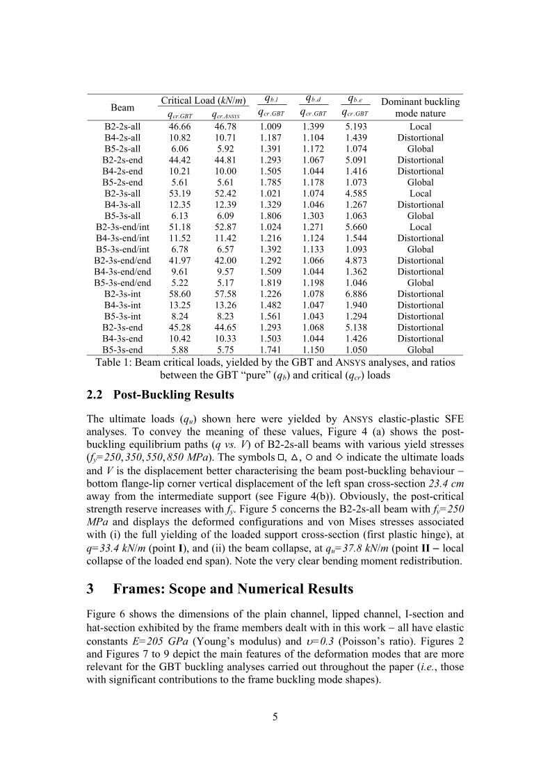
buckling modes, GBT analyses were carried out including only global (2-4), distortional (5-6) or local (7-17) deformation modes. Table 1 shows the critical load values, yielded by the ANSYS (qcr.ANSYS) and GBT (qcr.GBT − including all deformation modes) analyses, and the ratios between (i) the “pure” global (qb.e), distortional (qb.d) and local (qb.l) buckling loads − the “dominant buckling mode nature”, given in the last column, reflects the “closeness” between the associated “pure” buckling load and qcr.GBT (lowest of the three ratios).
Detail A
Detail B
A
B
L=5.0m
L=5.0m
-1.0
-0.5
0.0
0.5
1.0
0.0 2.5 5.0 7.5 10.0 12.5 15.0
3
3 4×(5)
4×(5)6 5
7×(5)
8×(5) 7×(5)
Length (m)
Figure 3: B5-3s-end/int beam critical buckling mode shapes yielded by ANSYS SFE and GBT analyses
Table 1: Beam critical loads, yielded by the GBT and ANSYS analyses, and ratios between the GBT “pure” (qb) and critical (qcr) loads
2.2 Post-Buckling Results The ultimate loads (qu) shown here were yielded by ANSYS elastic-plastic SFE analyses. To convey the meaning of these values, Figure 4 (a) shows the post-buckling equilibrium paths (q vs. V) of B2-2s-all beams with various yield stresses (fy=250, 350, 550, 850 MPa). The symbols , , and indicate the ultimate loads and V is the displacement better characterising the beam post-buckling behaviour − bottom flange-lip corner vertical displacement of the left span cross-section 23.4 cm away from the intermediate support (see Figure 4(b)). Obviously, the post-critical strength reserve increases with fy. Figure 5 concerns the B2-2s-all beam with fy=250 MPa and displays the deformed configurations and von Mises stresses associated with (i) the full yielding of the loaded support cross-section (first plastic hinge), at q=33.4 kN/m (point I), and (ii) the beam collapse, at qu=37.8 kN/m (point II − local collapse of the loaded end span). Note the very clear bending moment redistribution. 3 Frames: Scope and Numerical Results Figure 6 shows the dimensions of the plain channel, lipped channel, I-section and hat-section exhibited by the frame members dealt with in this work − all have elastic constants E=205 GPa (Young’s modulus) and υ=0.3 (Poisson’s ratio). Figures 2 and Figures 7 to 9 depict the main features of the deformation modes that are more relevant for the GBT buckling analyses carried out throughout the paper (i.e., those with significant contributions to the frame buckling mode shapes).
Figure 5: B2-2s-all beam deformed configuration and von Mises stresses − first
plastic hinge and beam collapse
20
60
150
200
4.0
5
60
Lipped channel I-sectionPlain channel
200
100
3.5
100
1.5
(mm)20
120
t
hat-section
Figure 6: Plain channel, lipped channel, I-section and hat-section dimensions
7
1 2 3 5 64 7 9 8
Global Local
Figure 7: Main features of the most relevant plain channel deformation modes
2 4 5 6 73 1 8 9 10
Global Local
Figure 8: Main features of the most relevant I-section deformation modes
7 8 9 10 2 3 4 5 6 1
Global Distortional Local
Figure 9: Main features of the most relevant hat-section deformation modes The buckling, post-buckling and ultimate strength results presented next concern the non-linear behaviours of the frames shown in Figures 10 to 13. Note that the geometries of these four frames were chosen in order to ensure buckling and failure modes involving all types of deformations (local, distortional and global).
The “L-shaped” plane frame depicted in Figure 10 (termed LF-U) is formed by two orthogonal short members exhibiting (i) identical plain channel cross-sections (see Figure 6), (ii) fixed end sections with warping prevented, and (iii) flange continuity at the joint (i.e., the two members are connected with their flanges lying in the same plane) − the members (A and B) have the same length (LA=LB=70cm) and are unequally axially compressed (NA=Q and NB=0.8Q, where Q is the load parameter) − naturally, this setting “forces” the collapse to occur in member A.
The symmetric orthogonal portal frame displayed in Figure 11 (termed PF-C) (i) is formed by three members with identical lipped channel cross-sections (see Figure 6), (ii) has fixed column bases and joints with flange continuity, and (iii) is acted by four loads applied at the joints and causing only first-order member axial forces (NA=NC=0.83Q and NB=Q).
Figure 12 shows a second “L-shaped” plane frame (termed LF-I), now formed by two fairly long members (LA=400cm and LB=600cm) exhibiting (i) identical I cross-sections (see Figure 6), (ii) again fixed end sections with warping prevented, and (iii) a box-stiffened joint (web continuity) − the frame is subjected to a vertical load Q applied at the beam mid-span cross-section centroid, causing essentially (i) bending in member B (beam) and (ii) bending and axial compression in member A (beam-column).
8
L =70cm
member A
A member B
B
L =70cm
YAX
XZ
BXQ
_
_
_
0.8Q
Figure 10: “L-shaped” frame formed by plain channel members (LF-U): geometry, loading and support conditions
L =50cm
member A
A
member B
B
L =
70cm
member C
Q0.83Q
0.83Q
Q
Figure 11: Symmetric portal frame formed by lipped channel members (PF-C): geometry, loading and support conditions
cL =
400c
m
BX
XA
bL =600cm Q bL /2
Y
Z X
θ >0
column
beam
BX
XA
column
beam
Figure 12: “L-shaped” frame formed by I-section members (LF-I): geometry, loading and support conditions
9
AL =
200c
m
L =300cmB
member A
member B
Qs.c
150cm
Y
Z X
θ >0
BX
XA
Figure 13: Symmetric portal frame formed by hat-section members (PF-Hat-1.5 and PF-Hat-2.5): geometry, loading and support conditions
The symmetric orthogonal portal frame displayed in Figure 13 (termed PF-Hat)
(i) is formed by three members with identical hat-section (see Figure 6), (ii) has fixed column bases and joints with web continuity, and (iii) is acted by a vertical load Q applied at the beam mid-span cross-section shear centre. Two different cross-section thicknesses are considered: t=1.5 mm (frame designated as PF-Hat-1.5) and t=2.5 mm (frame designated as PF-Hat-2.5).
3.1 Buckling Results Figures 14 to 18 provide two representations of critical buckling mode shapes of the frames considered in this work, namely (i) ANSYS 3D views and (ii) GBT modal amplitude functions. Table 2 shows (i) the frame critical buckling loads (Qcr) yielded by the ANSYS and GBT analyses (the latter include all deformation modes), and (ii) the ratios between the “pure buckling loads” (global, distortional and local − Qb.e, Qb.d and Qb.l) and Qcr.GBT. The frame “dominant buckling mode nature” corresponds to the smallest of these three ratios (i.e., to the “pure buckling load” closest to Qcr.GBT). The analysis of these frame buckling results prompts the following remarks: (i) The GBT and ANSYS critical buckling loads practically coincide − the maximum
difference is 3.7% and concerns the PF-Hat-1.5 frame. There is also very close agreement between the critical buckling mode representations provided by the two analyses.
10
(ii) While the LF-U frame buckles in a pure local mode, the SF-C, LF-I and PF-Hat frame critical buckling modes are “mixed”, in the sense that they combine at least two types of deformation modes: (ii1) local and distortional (PF-C and PF-Hat-1.5), (ii2) local and global (LF-I) or (ii3) local, distortional and global (PF-Hat-2.5).
(iii) The LF-U and PF-C frames can be more accurately described as sets of rigidly connected columns, since, in practical terms, all their members are axially compressed. Thus, they exhibit a “column-like” buckling behaviour that is triggered by the column with the “worst” combination of axial load and end support conditions: (iii1) member A in the LF-U case and (iii2) member B in the PF-C case.
(iv) The instability of the LF-I and PF-Hat-2.5 frames, which exhibit a “real frame behaviour” (columns subjected to axial compression and bending − beam-columns), are triggered by the lateral-torsional buckling of the beam (member B).
(v) In the PF-Hat-1.5 frame, all three members (columns and beam) share the responsibility of causing the frame buckling. This is because the major contributions of the distortional mode 5, which prevails in the frame critical buckling mode, occurs at the frame joint regions, which are subjected to high hogging moments − therefore, the cross-section lips located in these regions are under compression.
Figure 17: PF-Hat-1.5 frame: ANSYS and GBT critical buckling mode
representations
12
(vi) The critical buckling mode shapes of the LF-U and PF-C frames exhibit practically null joint deformations (i.e., displacements of the point corresponding to the intersection of the converging member centroidal axes). However, significant out-of-plane displacements, which stem from the beam lateral-torsional buckling (recall that the frame joints are not restrained against out-of-plane displacements), occur in the close vicinity of the LF-I and PF-Hat-2.5 frame joints.
-1.0
0.0
1.0
0 25 50 75 100 125 150 175 200
LA (cm)
3
4 6 8 × (2)
-1.0
0.0
1.0
0 50 100 150 200 250 300
LB (cm)
4
3
6
8 × (2)10 × (10)
3 4 6
8 10
Figure 18: PF-Hat-2.5 frame: ANSYS and GBT critical buckling mode
Table 2: Frame critical loads, yielded by the GBT and ANSYS analyses, and ratios
between the GBT “pure” (Qb) and critical (Qcr) loads
3.2 Post-Buckling Results This section addresses the SFE analysis of the elastic and elastic-plastic (for yield stress values equal to fy=250, 450, 650MPa) post-buckling behaviours of the LF-U, PF-C, LF-I, PF-hat-1.5 and PF-hat-2.5 frames. The curves shown in Figures 19(a) to 23(a) are the post-buckling equilibrium paths Q vs. vi and Q vs. θi, where (i) the
13
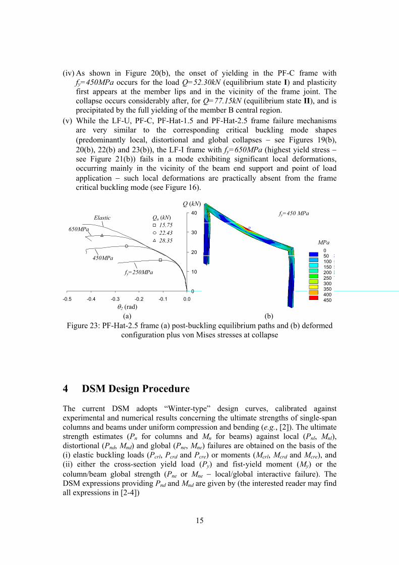
symbols , and identify the limit equilibrium states corresponding to the ultimate loads, (ii) v1, v2 and v3 are the transverse displacements of points P1 (LF-U frame), P2 (PF-C frame), P2 (PF-hat-1.5 frame), selected in order to provide a better frame post-buckling characterisation (Figures 19(a), 20(a) and 22(a) show the location of these points), and (iii) θ1 and θ2 are the torsional rotations of the beam mid-span cross-section of the LF-I and PF-hat-2.5 frames. As for Figures 19(b) to 23(b), they provide the failure modes and von Mises stress distributions of five frames: (i) LF-U frame with fy=250MPa, (ii) PF-C frame with fy=450MPa, (iii) LF-I frame with fy=650MPa, (iv) PF-hat-1.5 frame with fy=250MPa and (v) PF-hat-2.5 frame with fy=450MPa − note that Figure 20(b) also includes detailed information showing the onset of yielding. The observation of the post-buckling results shown in Figures 19 to 23 leads to the following conclusions:
(i) The amount of post-critical strength reserve increases with the yield stress (obviously) and in the frame sequence as LF-I (global buckling), PF-Hat-2.5 (global buckling), PF-C (distortional buckling), LF-U (local buckling) and PF-Hat-1.5 (distortional buckling). The higher post-critical strength reserve, occurring for the PF-Hat-1.5 frame with fy=650MPa, corresponds to an ultimate-to-critical load ratio equal to 3.2.
(ii) Increasing the yield stress from 250MPa to 650MPa leads to ultimate load increases of 81% (LF-U frames), 67% (PF-C frames), 47% (LF-I frames), 100% (PF-Hat-1.5 frames) and 80% (PF-Hat-2.5 frames).
(iii) The members responsible for the frame collapse are those triggering its instability, i.e., member A (LF-U frames), member B (PF-C frames) and the beam (LF-I, PF-Hat-1.5 and PF-Hat-2.5 frames).
(iv) As shown in Figure 20(b), the onset of yielding in the PF-C frame with fy=450MPa occurs for the load Q=52.30kN (equilibrium state I) and plasticity first appears at the member lips and in the vicinity of the frame joint. The collapse occurs considerably after, for Q=77.15kN (equilibrium state II), and is precipitated by the full yielding of the member B central region.
(v) While the LF-U, PF-C, PF-Hat-1.5 and PF-Hat-2.5 frame failure mechanisms are very similar to the corresponding critical buckling mode shapes (predominantly local, distortional and global collapses − see Figures 19(b), 20(b), 22(b) and 23(b)), the LF-I frame with fy=650MPa (highest yield stress − see Figure 21(b)) fails in a mode exhibiting significant local deformations, occurring mainly in the vicinity of the beam end support and point of load application − such local deformations are practically absent from the frame critical buckling mode (see Figure 16).
configuration plus von Mises stresses at collapse 4 DSM Design Procedure The current DSM adopts “Winter-type” design curves, calibrated against experimental and numerical results concerning the ultimate strengths of single-span columns and beams under uniform compression and bending (e.g., [2]). The ultimate strength estimates (Pn for columns and Mn for beams) against local (Pnl, Mnl), distortional (Pnd, Mnd) and global (Pne, Mne) failures are obtained on the basis of the (i) elastic buckling loads (Pcrl, Pcrd and Pcre) or moments (Mcrl, Mcrd and Mcre), and (ii) either the cross-section yield load (Py) and fist-yield moment (My) or the column/beam global strength (Pne or Mne − local/global interactive failure). The DSM expressions providing Pnd and Mnd are given by (the interested reader may find all expressions in [2-4])
16
ynd PP = if 0.561/. ≤= crdydc PPλ
yy
crd
y
crdnd P
PP
PPP
0.60.6
0.251 ⎟⎟⎠
⎞⎜⎜⎝
⎛⎟⎟
⎠
⎞
⎜⎜
⎝
⎛
⎟⎟⎠
⎞⎜⎜⎝
⎛−= if λc.d > 0.561 (1)
ynd MM = if 0.673/. ≤= crdydb MMλ
yy
crd
y
crdnd M
MM
MMM
5.05.0
22.01 ⎟⎟⎠
⎞⎜⎜⎝
⎛⎟⎟
⎠
⎞
⎜⎜
⎝
⎛
⎟⎟⎠
⎞⎜⎜⎝
⎛−= if 0.673. >dbλ . (2)
Note that these DSM curves neglect the (i) cross-section elastic-plastic strength reserve (statically determinate/indeterminate beams) and (ii) bending moment redistribution (statically indeterminate beams). Moreover, in frames, like in other structural systems or in single-span members not subjected to uniform compression or bending, the various “Pcr, Mcr and Py, My values” (i) cannot adequately describe the loading and (ii) need to be replaced by “first yield (qy or Qy) and critical buckling (qcr or Qcr) load factors” in the DSM equations.
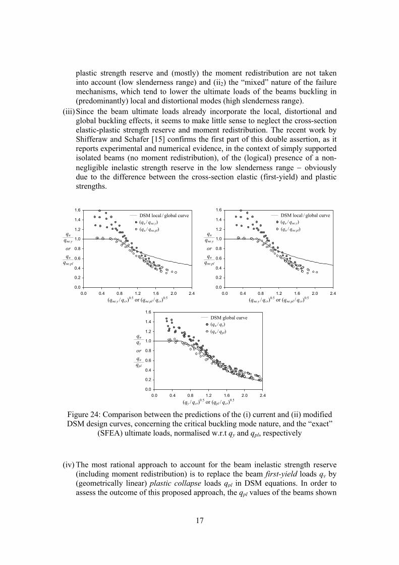
In this section, one presents an assessment of how accurately the continuous beam and frame ultimate strengths can be predicted by the current DSM design curves. 4.1 DSM Design of Continuous Beams Figure 24 shows comparisons between the ultimate strength predictions yielded by the current DSM design curves, selected on the basis of the beam critical buckling mode dominant nature (local, distortional or global), given in Table 1, and the “exact” values obtained through SFEA of the beams shown in Figure 1 with 15 different yield stresses, associated with yield-to-critical load ratios qy /qcr varying from 0.06 to 5.40 and covering a wide slenderness range – these results are summarised in table A1, presented later (in Appendix). The numerical (“exact”) ultimate loads, normalised w.r.t. qy, are identified by the dark dots. Although (i) the beams exhibit buckling/failure modes that are not “pure” and (ii) the DSM curve choice was based on their “dominant buckling mode nature”, it is worth noting that slenderness values are evaluated with the “real” beam critical buckling load qcr, which is not “purely” local, distortional or global. The observation of these results/comparisons prompts the following remarks: (i) When normalised w.r.t qy, the DSM predictions are (i1) excessively safe in the
low slenderness range, (i2) safe and reasonable accurate in the intermediate slenderness range and (i3) clearly unsafe (local/distortional) or safe and accurate (global) in the high slenderness range.
(ii) None of the three DSM design curves provides efficient (safe and economic) predictions of the continuous beam ultimate loads over the whole slenderness range. This is due to a combination of factors: (ii1) both the cross-section elastic-
17
plastic strength reserve and (mostly) the moment redistribution are not taken into account (low slenderness range) and (ii2) the “mixed” nature of the failure mechanisms, which tend to lower the ultimate loads of the beams buckling in (predominantly) local and distortional modes (high slenderness range).
(iii) Since the beam ultimate loads already incorporate the local, distortional and global buckling effects, it seems to make little sense to neglect the cross-section elastic-plastic strength reserve and moment redistribution. The recent work by Shifferaw and Schafer [15] confirms the first part of this double assertion, as it reports experimental and numerical evidence, in the context of simply supported isolated beams (no moment redistribution), of the (logical) presence of a non-negligible inelastic strength reserve in the low slenderness range − obviously due to the difference between the cross-section elastic (first-yield) and plastic strengths.
0.0
0.2
0.4
0.6
0.8
1.0
1.2
1.4
1.6
0.0 0.4 0.8 1.2 1.6 2.0 2.4
DSM local / global curve(qu / qne.y)
(qne.y / qcr)0.5 or (qne.pl / qcr)0.5
qne.y qu
(qu / qne.pl)
qne.pl qu or
0.0
0.2
0.4
0.6
0.8
1.0
1.2
1.4
1.6
0.0 0.4 0.8 1.2 1.6 2.0 2.4
DSM local / global curve(qu / qne.y)
(qne.y / qcr)0.5 or (qne.pl / qcr)0.5
qne.y
qu (qu / qne.pl)
qne.pl
qu or
0.0
0.2
0.4
0.6
0.8
1.0
1.2
1.4
1.6
0.0 0.4 0.8 1.2 1.6 2.0 2.4
DSM global curve (qu / qy)
(qy / qcr)0.5 or (qpl / qcr)0.5
qy qu
(qu / qpl)
qpl qu or
Figure 24: Comparison between the predictions of the (i) current and (ii) modified DSM design curves, concerning the critical buckling mode nature, and the “exact”
(SFEA) ultimate loads, normalised w.r.t qy and qpl, respectively
(iv) The most rational approach to account for the beam inelastic strength reserve
(including moment redistribution) is to replace the beam first-yield loads qy by (geometrically linear) plastic collapse loads qpl in DSM equations. In order to assess the outcome of this proposed approach, the qpl values of the beams shown
18
in Figure 1, all analysed with 15 different yield stresses, were obtained through first-order elastic-plastic SFEA carried out in the code ANSYS (these values are given in table A1). Figure 24 also compares the ultimate load predictions yielded by these modified DSM design curves and the previous SFE ultimate loads, now normalised w.r.t. qpl and represented by white dots. The observation of these new comparisons leads to the following comments: (iv1) In the low slenderness range (λcr<0.7), the modified (normalized w.r.t. qpl)
DSM predictions are quite accurate (only a few are marginally unsafe), which confirms the presence and relevance of the beam inelastic strength reserve (cross-section plastic strength and moment redistribution).
(iv2) In the intermediate slenderness range (0.7<λcr<1.2), most of the modified DSM predictions are fairly accurate, even if there are a number of slightly unsafe estimates.
(iv3) In the high slenderness range (λcr >1.2), the current and modified DSM predictions practically coincide: they are both unsafe (local and distortional) or slightly safe (global).
(v) One general and interesting result consists of the fact that, in the high critical slenderness range (λcr>1.2), the elastic buckling curve predicts rather accurately the beam ultimate strength, regardless of the buckling mode dominant nature − this is clearly shown in Figure 25.
0.0
0.2
0.4
0.6
0.8
1.0
1.2
1.4
1.6
0.0 0.4 0.8 1.2 1.6 2.0 2.4 (qpl / qcr)0.5
qpl qu
Elastic bucklingDominant buckling mode nature:
LocalDistortionalGlobal
Figure 25: Comparison between the elastic buckling curve and the SFE ultimate loads
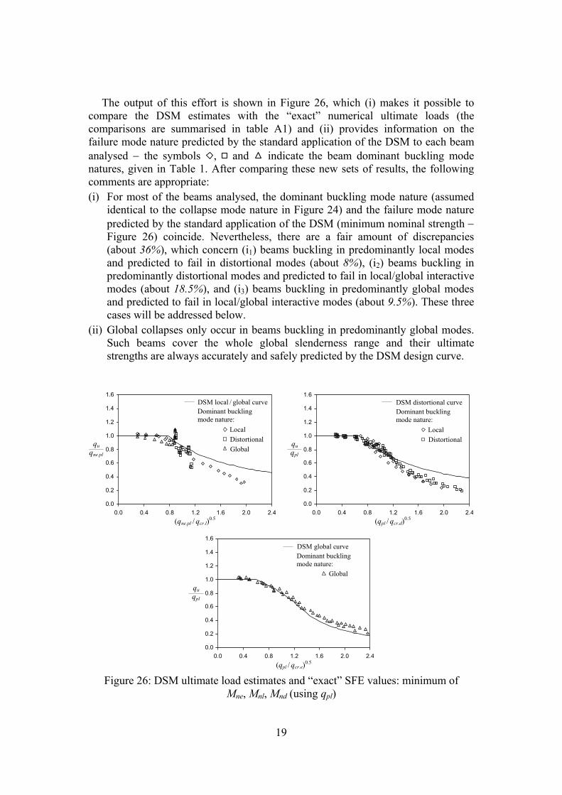
When at least two “pure” buckling loads (i.e., qb.e, qb.d, qb.l) are close, the failure mode and “dominant buckling mode” natures may be different. This observation can be confirmed, for instance, by looking at the buckling and collapse modes of the beam B2-2s-all with fy=250MPa – while the buckling mode is predominantly local (see table 1), its collapse mechanism involves mostly distortional deformations (see Figure 5). Therefore, it was decided to include qpl in the standard (adequate) usual application of the DSM, in which the ultimate loads are estimated using the minimum of the nominal strengths qne, qnl and qnd, combined with the slenderness value associated with qcr.i = (qb.i / qb.min) qcr, where qb.min = min {qbe, qbd, qbl} − this amounts to assuming that the ratios between the bifurcation loads associated with “pure” and “impure” buckling mode natures are the same.
19
The output of this effort is shown in Figure 26, which (i) makes it possible to compare the DSM estimates with the “exact” numerical ultimate loads (the comparisons are summarised in table A1) and (ii) provides information on the failure mode nature predicted by the standard application of the DSM to each beam analysed − the symbols , and indicate the beam dominant buckling mode natures, given in Table 1. After comparing these new sets of results, the following comments are appropriate: (i) For most of the beams analysed, the dominant buckling mode nature (assumed
identical to the collapse mode nature in Figure 24) and the failure mode nature predicted by the standard application of the DSM (minimum nominal strength − Figure 26) coincide. Nevertheless, there are a fair amount of discrepancies (about 36%), which concern (i1) beams buckling in predominantly local modes and predicted to fail in distortional modes (about 8%), (i2) beams buckling in predominantly distortional modes and predicted to fail in local/global interactive modes (about 18.5%), and (i3) beams buckling in predominantly global modes and predicted to fail in local/global interactive modes (about 9.5%). These three cases will be addressed below.
(ii) Global collapses only occur in beams buckling in predominantly global modes. Such beams cover the whole global slenderness range and their ultimate strengths are always accurately and safely predicted by the DSM design curve.
0.0
0.2
0.4
0.6
0.8
1.0
1.2
1.4
1.6
0.0 0.4 0.8 1.2 1.6 2.0 2.4
DSM local / global curve
(qne.pl / qcr.l)0.5
qne.pl qu
Dominant buckling mode nature:
LocalDistortionalGlobal
0.0
0.2
0.4
0.6
0.8
1.0
1.2
1.4
1.6
0.0 0.4 0.8 1.2 1.6 2.0 2.4
DSM distortional curve
(qpl / qcr.d)0.5
qpl qu
Dominant buckling mode nature:
Local Distortional
0.0
0.2
0.4
0.6
0.8
1.0
1.2
1.4
1.6
0.0 0.4 0.8 1.2 1.6 2.0 2.4
DSM global curve
(qpl / qcr.e)0.5
qpl qu
Dominant buckling mode nature:
Global
Figure 26: DSM ultimate load estimates and “exact” SFE values: minimum of
Mne, Mnl, Mnd (using qpl)
20
(iii) The DSM estimates shown in Figures 24 and 26 practically coincide (differences below 4%) for the beams (iii1) buckling in predominantly local modes and predicted to fail in distortional modes, regardless of the local/global critical slenderness value, (iii2) buckling in predominantly distortional modes and predicted to fail in local/global modes, for moderate distortional critical slenderness values (1.0 <λcr < 1.2) and (iii3) buckling in predominantly global modes and predicted to fail in local/global modes, for low-to-moderate global critical slenderness values (λcr <1.2). In the first case, the ultimate strengths are either (iii1) fairly accurately predicted (low-to-moderate critical slenderness) or (iii2) clearly overestimated (high critical slenderness). In the second case, the ultimate strength estimates are slightly unsafe. Finally, in the last case, the ultimate load predictions are moderately or slightly unsafe.
(iv) The larger differences between the DSM estimates shown in Figures 24 and 26 occur for beams buckling in predominantly distortional modes that (iv1) exhibit high critical slenderness values (λcr>1.2) and (iv2) are predicted to fail in local/global interactive modes (with moderate slenderness values). Such differences (drops in ultimate load estimates) may reach 93% and their average is about 34%, which means that they are highly scattered. In these cases, the ultimate load predictions yielded by the standard application of the DSM (Figure 26) are closer to the SFEA results, although not as accurate as those provided by the elastic buckling curve (see Table A1).
(v) The larger differences between the DSM estimates shown in Figures 24 and 26 occur for beams buckling in predominantly distortional modes that (iv1) exhibit high critical slenderness values (λcr>1.2) and (iv2) are predicted to fail in local/global. For the beams buckling in predominantly global modes, with high critical slenderness values (λcr>1.2), and predicted to fail in local/global interactive modes, the ultimate load predictions drop by about 8% − they change from “practically exact” to “slightly safe” and exhibit much lower local/global slenderness values.
fy=850MPa fy=450MPa B5-3s-end/int B5-3s-int
Figure 27: Failure modes of the B5-3s-end/int beam with fy=850MPa and B5-3s-int
beam with fy=450MPa (SFEA)
21
(vi) In some cases, the collapse mode nature predicted by the standard application of the DSM does not match that obtained through the SFEA. For instance, consider the B5-3s-int beam with fy=450MPa and the B5-3s-end/int beam with fy=850MPa: while the failure mechanisms observed in the SFEA (see Figure 27) coincide with the dominant buckling mode natures (global and distortional, respectively), those predicted by the standard application of the DSM are local/global in both beams.
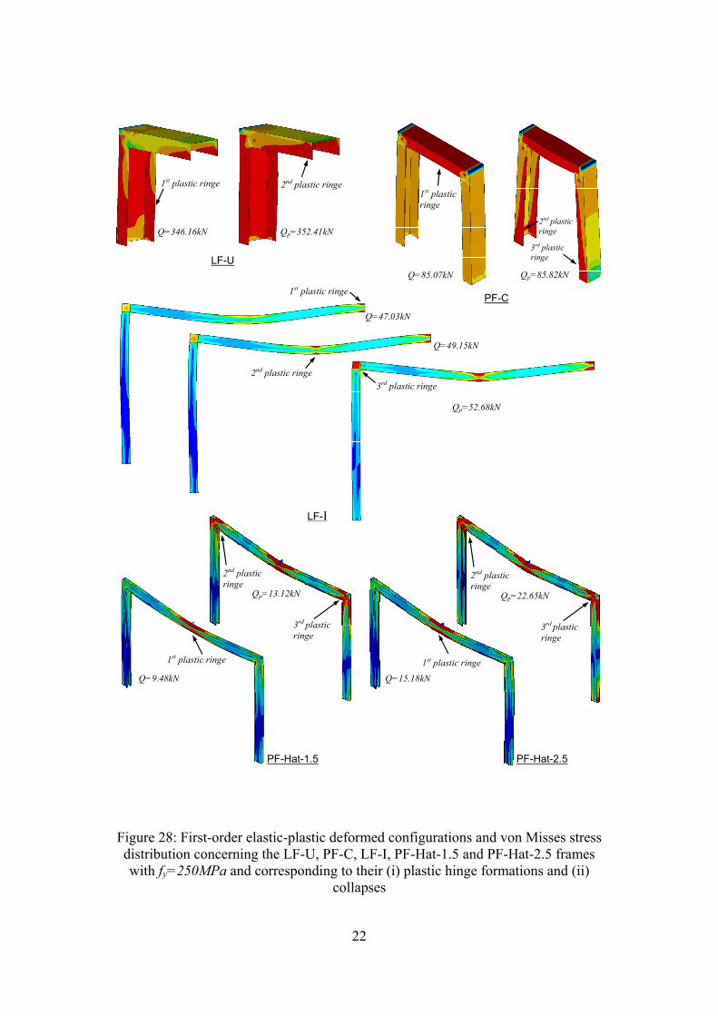
4.2 DSM Design of Simple Frames In order to be able to assess the quality of the frame ultimate strength estimates provided by the modified DSM approach, the first step consists of determining the Qpl values for the LF-U, PF-C, LF-I, PF-Hat-1.5 and PF-Hat-2.5 frames, all assumed to exhibit 6 different yield stresses, namely fy=250, 300, 350, 450, 550, 650 MPa. These Qpl values were obtained through first-order elastic-plastic ANSYS SFEA and are given in Table 3. For illustrative purposes, Figure 28 displays deformed configurations and von Mises stress distributions, concerning the five frames analysed and fy=250MPa, which are associated with (i) the formation of the successive “plastic hinges” (cross-section full yielding) and (ii) the frame collapse. Note that the members triggering the frame instabilities are again those also responsible for their (first-order) plastic collapses. Moreover, since the LF-U and PF-C frame members are almost exclusively subjected to axial compression, the corresponding first plastic hinge locations are not well defined at all − indeed, full yielding occurs practically at the same time in a whole member “region”. Conversely, the first plastic hinge occurs at a very well defined location in the LF-I and PF-Hat frames: the (i) beam end support (LF-I frame) or (ii) beam mid-span (PF-Hat-1.5 and PF-Hat-2.5 frames) − in such cases, instability and collapse stem mainly from beam non-uniform bending.
Next, the ultimate load estimates yielded by the modified DSM approach are compared with the ANSYS SFE values, for the five frames with yield stresses fy=250,
300, 350, 450, 550, 650 MPa. As mentioned earlier, the current DSM prescribes different strength curve sets for columns and beams [2-4]. In this work, the DSM curve set selection was based on the member triggering the frame instability and collapse (the same in all cases). This means that DSM column strength curves to be considered concern (i) columns for the LF-U and PF-C frames, and (ii) beams for the LF-I, PF-Hat-1.5 and PF-Hat-2.5 frames1.
1 Note that, since the current DSM does not cover beam-columns, the DSM strength curve selection procedure
employed in this work would be “irreparably compromised” if the instability and collapse of the LF-I and PF-Hat frames was triggered by member A, which is a beam-column subjected to a high compressive axial force − at least, until DSM beam-column strength curves are developed and adequately validated. On the other hand, note that the compressive axial forces acting on the LF-I and PF-Hat frame beams are quite small, which justifies why they were disregarded when the DSM curve for beams was selected.
22
1st plastic ringe 2nd plastic ringe
Q=346.16kN Qp=352.41kN
1st plastic ringe
2nd plastic ringe
3rd plastic ringe
Q=85.07kN Qp=85.82kN
1st plastic ringe
2nd plastic ringe 3rd plastic ringe
Q=47.03kN
Q=49.15kN
Qp=52.68kN
LF-U
PF-C
LF-I
1st plastic ringe
2nd plastic ringe
3rd plasticringe
Q=9.48kN
Qp=13.12kN
PF-Hat-1.5
Q=15.18kN
1st plastic ringe
2nd plastic ringe
3rd plastic ringe
Qp=22.65kN
PF-Hat-2.5
Figure 28: First-order elastic-plastic deformed configurations and von Misses stress distribution concerning the LF-U, PF-C, LF-I, PF-Hat-1.5 and PF-Hat-2.5 frames with fy=250MPa and corresponding to their (i) plastic hinge formations and (ii)
collapses
23
SFEA DSM
fy
(MPa) DBN plQ
(kN) uQ
(kN) plcr.λ DSMuQ .
(kN)
*.DSMuQ
(kN)
FMNu
DSMu
QQ .
u
DSMu
QQ*
.
LF-U
250 L 352.41 263.06 1.18 264.95 264.95 L/G 1.01 1.01
300 L 423.12 293.79 1.29 298.01 298.01 L/G 1.01 1.01
350 L 493.03 322.72 1.39 328.47 328.47 L/G 1.02 1.02
450 L 634.64 377.27 1.58 384.86 384.86 L/G 1.02 1.02
550 L 774.28 428.19 1.74 435.16 435.16 L/G 1.02 1.02
650 L 916.78 476.28 1.90 482.29 482.29 L/G 1.01 1.01
PF-
C
250 D 85.82 55.90 1.29 51.62 51.62 D 0.92 0.92
300 D 103.67 61.69 1.42 57.02 57.02 D 0.92 0.92
350 D 121.07 66.81 1.53 61.74 61.74 D 0.92 0.92
450 D 155.89 77.15 1.74 70.00 70.00 D 0.91 0.91
550 D 190.27 85.82 1.92 77.07 77.07 D 0.90 0.90
650 D 224.64 93.40 2.09 83.38 83.38 D 0.89 0.89
LF-I
250 G 52.68 34.81 1.01 41.84 41.84 G 1.20 1.20
300 G 63.54 38.79 1.11 46.32 46.32 G 1.19 1.19
350 G 73.36 41.10 1.20 49.14 49.14 G 1.20 1.20
450 G 93.39 44.87 1.35 51.32 50.90 L/G 1.14 1.13
550 G 115.89 46.99 1.50 51.32 50.90 L/G 1.09 1.08
650 G 137.10 51.10 1.63 51.32 50.90 L/G 1.01 1.00
PF-
Hat
-1.5
250 D 13.12 8.31 1.60 7.07 7.07 D 0.85 0.85
300 D 15.84 9.67 1.76 7.88 7.88 D 0.82 0.82
350 D 18.39 10.99 1.89 8.58 8.58 D 0.78 0.78
450 D 23.43 13.36 2.14 9.83 9.83 D 0.74 0.73
550 D 29.18 15.41 2.38 11.11 11.11 D 0.72 0.63
650 D 34.18 16.69 2.58 12.11 12.11 D 0.73 0.58
PF-
Hat
-2.5
250 G 22.65 15.75 1.10 16.78 16.78 G 1.07 1.07
300 G 26.84 17.60 1.19 18.05 18.05 G 1.03 1.03
350 G 31.18 19.60 1.28 18.76 18.76 G 0.96 0.96
450 G 39.68 22.93 1.45 18.89 18.89 G 0.82 0.82
550 G 49.18 25.84 1.61 18.89 18.89 G 0.73 0.73
650 G 57.68 28.35 1.75 18.89 18.89 G 0.67 0.67
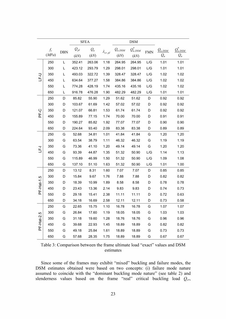
Table 3: Comparison between the frame ultimate load “exact” values and DSM estimates
Since some of the frames may exhibit “mixed” buckling and failure modes, the
DSM estimates obtained were based on two concepts: (i) failure mode nature assumed to coincide with the “dominant buckling mode nature” (see table 2) and slenderness values based on the frame “real” critical buckling load Qcr,
24
corresponding to a “mixed” buckling mode (not local, distortional or global), and (ii) lower of Qne, Qnl, Qnd and the three slenderness values based on Qcr.i=(Qb.i /Qb.min) ×
Qcr, where Qb.min=min {Qb.e, Qb.d, Qb.l} − usual DSM application. Table 3 provides, for all the frames analysed, the following values: (i) first-order plastic collapse (Qpl) and ultimate (Qu) loads, (ii) critical slenderness values (λcr.pl), obtained from Qcr (given in section 3.1) and Qpl, (iii) ultimate load estimates yielded by the current DSM design curves (iii1) selected on the basis of the dominant buckling nature (Qu.DSM) and (iii2) corresponding to the lower of Qne, Qnl, Qnd ( *
.DSMuQ ). Moreover, this table provides also (i) the dominant buckling natures (DBN), (ii) the failure mode natures predicted by the DSM (FMN) and (iii) the values of the ratios Qu.DSM
/Qu.. On the other hand, Figures 29(a) and 29(b) make it possible to compare the above two sets of DSM estimates with the values obtained by means of the ANSYS SFE analyses.
The observation of the results presented in Table 3 and Figures 29(a) and 29(b) prompts the following comments and remarks, concerning the “quality” of the DSM-based frame ultimate strength estimates:
(i) The comparison between the SFE ultimate load values and the corresponding DSM estimates based on the “dominant buckling mode nature”, both of which are displayed in Figure 29(a), makes it possible to conclude that (i1) the LF-U frame predictions (local instability/collapse) are all very accurate, even if minutely unsafe (Qu.DSM /Qu values varying between 1.01 and 1.02), (i2) the PF-C frame predictions (distortional instability/collapse) are all safe, even if only reasonable accurate (Qu.DSM /Qu values varying between 0.89 and 0.92), (i3) the LF-I frame predictions (global instability/ collapse) are practically all fairly or excessively unsafe (with a single exception, which corresponds to a “perfect” estimate, the Qu.DSM /Qu values vary between 1.09 and 1.20), (i4) the PF-Hat-1.5 frame predictions (distortional instability/collapse) are all excessively safe (Qu.DSM /Qu values varying between 0.73 and 0.85) and (i5) the PF-Hat-2.5 frame predictions (global instability/collapse) are either reasonably accurate or excessively safe (Qu.DSM /Qu values varying between 0.67 and 1.07).
(ii) The adoption of the lower of the Qne, Qnl, Qnd values as the frame ultimate strength estimate only leads to a change in three LF-I frames, namely those associated with higher slenderness values, i.e., yield stresses. They correspond to the points labeled 1-3 in the bottom plot of Figure 29(a) , which are found to “migrate” to the bottom plot of Figure 29(b), thus meaning that the current DSM application predicts local/global interactive failures for these three frames. Note also that their slenderness values, which change from global to local, (ii1) are substantially reduced and (ii2) become identical, which stems from the fact that Qne=Qcre for λb.e>1.336 and, thus, λb.l=(Qcre/Qcrl)0.5 is constant.
(iii) Since Qcrl is considerably larger than Qcre for the three frames identified in the previous item, the local/global interaction effects are rather weak, which explains the extreme closeness between the *
.DSMuQ and Qu.DSM values, leading to (minuscule) differences in the corresponding ultimate strength ratios (see Table 3) − the *
.DSMuQ values are a touch below the Qu.DSM ones. So, in this particular
25
0.0
0.2
0.4
0.6
0.8
1.0
1.2
0.0 0.5 1.0 1.5 2.0 2.5
(Qne /Qcr)0.5
Qne Qu
DSM local / global curvefor columns and beams LF-U (Qu /Qne)
0.0
0.2
0.4
0.6
0.8
1.0
1.2
0.0 0.5 1.0 1.5 2.0 2.5
(Qne.pl /Qcr.l)0.5
Qne.pl
Qu
Dominant bucklingmode nature:
Local Global1 2
3
DSM local / global curvefor columns and beams
0.0
0.2
0.4
0.6
0.8
1.0
1.2
0.0 0.5 1.0 1.5 2.0 2.5
(Qpl /Qcr)0.5
Qpl Qu
PF-C (Qu /Qpl)
DSM distortional curvefor columns
0.0
0.2
0.4
0.6
0.8
1.0
1.2
0.0 0.5 1.0 1.5 2.0 2.5
(Qpl /Qcr.d)0.5
Qpl
Qu
Dominant bucklingmode nature:
Distortional
DSM distortional curvefor columns
0.0
0.2
0.4
0.6
0.8
1.0
1.2
0.0 0.4 0.8 1.2 1.6 2.0 2.4 2.8
(Qpl /Qcr)0.5
Qpl Qu
PF-Hat-1.5 (Qu /Qpl)
DSM distortional curvefor beams
0.0
0.2
0.4
0.6
0.8
1.0
1.2
0.0 0.4 0.8 1.2 1.6 2.0 2.4 2.8
(Qpl /Qcr.d)0.5
Qpl
Qu
Dominant bucklingmode nature:
Distortional
DSM distortional curvefor beams
0.0
0.2
0.4
0.6
0.8
1.0
1.2
0.0 0.5 1.0 1.5 2.0 2.5
(Qpl /Qcr)0.5
Qpl Qu
LF-I (Qu /Qpl)
1 2 3
DSM global curve for beams
PF-Hat-2.5
0.0
0.2
0.4
0.6
0.8
1.0
1.2
0.0 0.5 1.0 1.5 2.0 2.5
(Qpl / Qcr.e)0.5
Qpl
Qu
Dominant bucklingmode nature:
Global
DSM global curvefor beams
(a) (b)
Figure 29: DSM ultimate load estimates and SFE analyses: (a) “dominant buckling mode nature” and “minimum of Qne, Qnl, Qnd”
26
case, the DSM global and local/global interactive strength curves predict essentially the same failure loads, but on the basis of distinct slenderness values.
(iv) The natures of the collapse modes displayed in Figures 19 to 23 confirm the DSM predictions. Indeed, (iv1) the first two frames (LF-U and PF-C frames) exhibit pure local and distortional collapse modes, respectively, (iv2) the third (LF-I frame with fy=650 MPa frame) one fails in a mode that combines local and global (flexural-torsional) deformations and (iv3) the last two frames (PF-Hat-1.5 and PF-Hat-2.5 frames) exhibit distortional and global collapse modes, respectively.
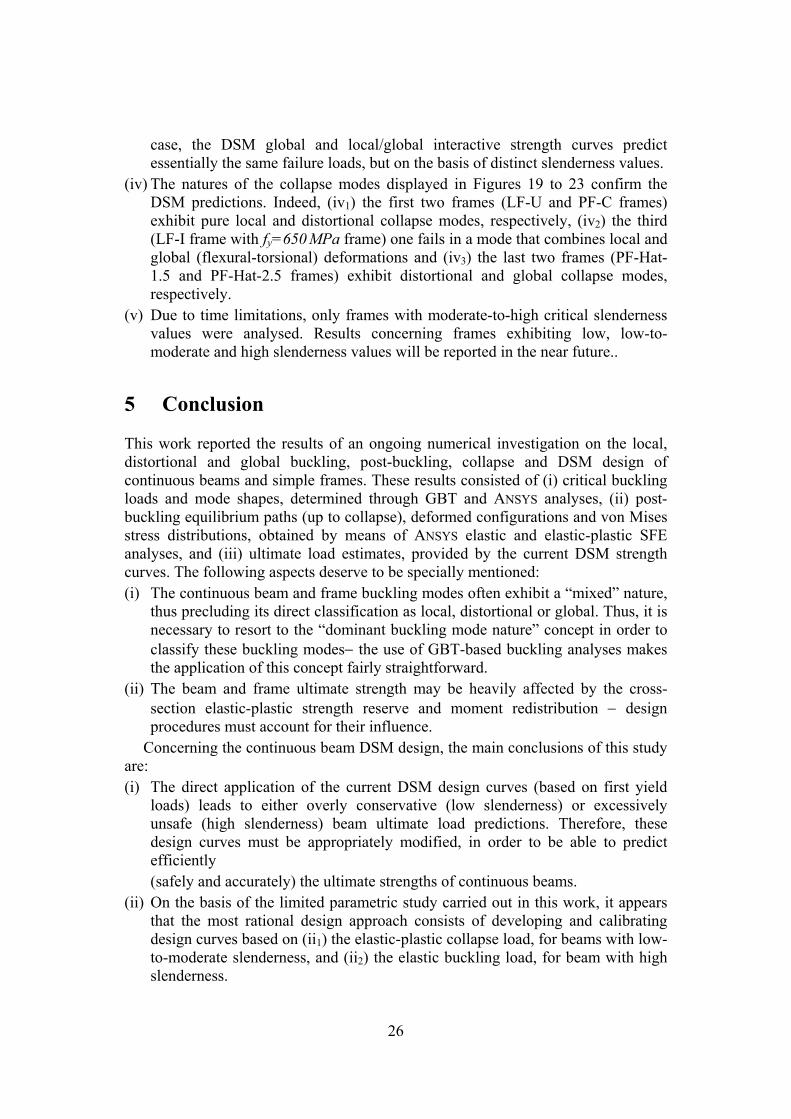
(v) Due to time limitations, only frames with moderate-to-high critical slenderness values were analysed. Results concerning frames exhibiting low, low-to-moderate and high slenderness values will be reported in the near future..
5 Conclusion This work reported the results of an ongoing numerical investigation on the local, distortional and global buckling, post-buckling, collapse and DSM design of continuous beams and simple frames. These results consisted of (i) critical buckling loads and mode shapes, determined through GBT and ANSYS analyses, (ii) post-buckling equilibrium paths (up to collapse), deformed configurations and von Mises stress distributions, obtained by means of ANSYS elastic and elastic-plastic SFE analyses, and (iii) ultimate load estimates, provided by the current DSM strength curves. The following aspects deserve to be specially mentioned: (i) The continuous beam and frame buckling modes often exhibit a “mixed” nature,
thus precluding its direct classification as local, distortional or global. Thus, it is necessary to resort to the “dominant buckling mode nature” concept in order to classify these buckling modes− the use of GBT-based buckling analyses makes the application of this concept fairly straightforward.
(ii) The beam and frame ultimate strength may be heavily affected by the cross-section elastic-plastic strength reserve and moment redistribution − design procedures must account for their influence.
Concerning the continuous beam DSM design, the main conclusions of this study are: (i) The direct application of the current DSM design curves (based on first yield
loads) leads to either overly conservative (low slenderness) or excessively unsafe (high slenderness) beam ultimate load predictions. Therefore, these design curves must be appropriately modified, in order to be able to predict efficiently
(safely and accurately) the ultimate strengths of continuous beams. (ii) On the basis of the limited parametric study carried out in this work, it appears
that the most rational design approach consists of developing and calibrating design curves based on (ii1) the elastic-plastic collapse load, for beams with low-to-moderate slenderness, and (ii2) the elastic buckling load, for beam with high slenderness.
27
As far as the frame DSM design is concerned, the following issues are relevant: (i) Since the (modified) current DSM strength curves were developed and validated
in the context of isolated columns or beams, it was expected that they would only provide satisfactory (safe and reasonably accurate) ultimate strength estimates in frames that buckle and fail in modes triggered by members subjected almost exclusively to pre-buckling axial compression (columns) or bending (beams) − i.e., not beam-columns (members subjected to pre-buckling axial compression and bending).
(ii) Indeed, the current DSM design curves are not able to predict accurately the ultimate strength of frames (ii1) containing members subjected to bending and high compression (“clear beam-columns”) or (ii2) whose buckling and failure modes involve considerable joint deformations. In such cases, new/modified DSM design curves must be developed and calibrated − in this respect, note that the existing DSM design curves do not cover yet isolated beam-columns (this is a subject of current research).
Acknowledgements The financial support of Fundação para a Ciência e Tecnologia (FCT − Portugal), through project PTDC/ECM/108146/2008, and Fundação de Amparo à Pesquisa do Estado de São Paulo (FAPESP – Brazil), through project 11/15731-5, is gratefully acknowledged. The first author also acknowledges FAPESP for his postdoctoral scholarship, 2011/17557-2. References [1] D. Dubina, “Structural analysis and design assisted by testing of cold-formed
steel structures”, Thin-Walled Structures, 46(7-9), 741-764, 2008. [2] B.W. Schafer, “Review: the direct strength method of cold-formed steel
member design”, Journal of Constructional Steel Research, 64(7-8), 766-778, 2008.
[3] Standards of Australia and Standards of New Zealand (SA-SNZ), Australian/New Zealand Standard on Cold-Formed Steel Structures − AS/NZS 4600 (2nd edition), Sydney-Wellington, 2005.
[4] American Iron and Steel Institute (AISI), North American Specification for the Design of Cold-Formed Steel Structural Members − NAS: AISI-S100-07, Washington (DC), 2007.
[5] C. Yu and B.W. Schafer, “Simulation of cold-formed steel beams in local and distortional buckling with applications to the direct strength method”, Journal of Constructional Steel Research, 63(5), 581-590, 2007.
[6] D. Camotim, N. Silvestre, C. Basaglia and R. Bebiano R., “GBT-based buckling analysis of thin-walled members with non-standard support conditions”, Thin-Walled Structures, 46(7-9), 800-815, 2008.
[7] C. H. Pham and G. Hancock, “Direct strength design of cold-formed purlins”, Journal of Structural Engineering, 135(3), 229-238, 2009.
28
[8] C. Basaglia, D. Camotim, N. Silvestre N, “Torsion warping transmission at thin-walled frame joints: kinematics, modelling and structural response”, Journal of Construction Steel Research, 69, 39-53, 2012.
[9] C. Basaglia, D. Camotim, N. Silvestre, “GBT-Based Buckling Analysis of Thin-Walled Steel Frames with Arbitrary Loading and Support Conditions”, International Journal of Structural Stability and Dynamics, 10(3), 363-385, 2010.
[10] D. Camotim, C. Basaglia, N. Silvestre, “GBT buckling analysis of thin-walled steel frames: a state-of-the-art report”, Thin-Walled Structures, 48(10-11), 726-743, 2012.
[11] Comité Européan de Normalization (CEN), Eurocode 3 − Design of Steel Structures − Part 1-1: General Rules and Rules for Buildings, EN1993-1-1, Brussels, 2005.
[12] F. Bijlaard, M. Feldmann, J. Naumes, G. Sedlacek, “The “general method” for assessing the out-of-plane stability of structural members and frames and the comparison with alternative rules in EN 1993 – Eurocode 3 – Part 1-1”, Steel Construction − Design and Research, 3(1), 19-33, 2010.
[13] Swanson Analysis Systems Inc., ANSYS Reference Manual (version 12), 2009. [14] C. Basaglia, D. Camotim, “Buckling, post-buckling, strength and DSM design
of cold-formed steel continuous lipped channel beams”, Journal of Structural Engineering (ASCE), 2012, accepted for publication.
[15] Y. Shifferaw and B.W. Schafer, “Inelastic bending capacity in cold-formed steel members”, Proceedings of Structural Stability Research Council Annual Stability Conference (New Orleans, 18-21/4), 279-299, 2007.
Appendix Table A1 shows, for all the continuous beams analysed, the values of (i) the first yield (qy), plastic collapse (qpl) and ultimate (qu) loads, (ii) the ultimate load estimates yielded by the DSM design curves (ii1) selected on the basis of the dominant buckling mode nature, using qy (qu.DSM.y) or qpl (qu.DSM.pl), and (ii2) corresponding to the DSM standard application, using qpl ( *
.. plDSMuq ). Moreover, the table provides (i) the dominant buckling mode natures (BN), (ii) the failure mode natures predicted by the DSM (FM) and (iii) the values of the ratios qu.DSM /qu and qcr
/qu − the averages and standard deviations of these ratios, for low (λ<0.7), moderate (0.7<λ<1.2) and high (λ > 1.2) slenderness values, are also presented. However, since the first-order plastic collapse of the beams B_-3s-end/end involves the full yielding of their intermediate spans (under uniform bending, both before and after the formation of the first plastic hinge), numerical convergence problems precluded the determination of the corresponding qpl values. Due to lack of time to find a procedure to overcome these convergence problems (one possible way, not yet tested, is to consider marginally different distributed loads in the two beam end spans, thus leading to a “slightly non-uniform” bending moment diagram in the intermediate span), the comparisons requiring the qpl values are not presented here for the above beams.