TITLE: BUDGET VARIANCES IN INSURANCE COMPANY OPERATIONS AUTHOR: Hr. George M. Levine Mr. Levine is employed by the National Council on Compensation Insurance. He received his B.S. degree from the University of Pennsylvania's Wharton School, with a double major in Actuarial Science and Accounting. George received his ACAS in 1982 and is a member of the American Academy of Actuaries. ABSTRACT: This paper attempts to provide the actuary with a methodology for monitoring the price and quantity of insurance for budgeting purposes. The paper discusses and defines cost accounting concepts and relates them to casualty actuarial work. The technique entitled "Analysis of Budget Variances" is applied to budgeted figures and actual results displayed on a net income statement prepared using the contribution method of allocating expenses. Although this process is shown to have applications for the assignment of responsibility for budget variances, its main contribution is to provide a separation of the variances of components of the net income statement into their price and quantity variances. -243 -
Transcript
TITLE: BUDGET VARIANCES IN INSURANCE COMPANY OPERATIONS
AUTHOR: Hr. George M. Levine
Mr. Levine is employed by the National Council on Compensation Insurance. He received his B.S. degree from the University of Pennsylvania's Wharton School, with a double major in Actuarial Science and Accounting. George received his ACAS in 1982 and is a member of the American Academy of Actuaries.
ABSTRACT:
This paper attempts to provide the actuary with a methodology for monitoring the price and quantity of insurance for budgeting purposes. The paper discusses and defines cost accounting concepts and relates them to casualty actuarial work. The technique entitled "Analysis of Budget Variances" is applied to budgeted figures and actual results displayed on a net income statement prepared using the contribution method of allocating expenses. Although this process is shown to have applications for the assignment of responsibility for budget variances, its main contribution is to provide a separation of the variances of components of the net income statement into their price and quantity variances.
-243 -
The need for explaining variances from budgeted results is a concern for
casualty actuaries in insurance companies. Often, the method of presentation is the
determination of an "indication," which shows the rate change necessary to balance
the actual historical loss ratio with the expected, or budgeted, loss ratio.
The "indicated rate change" evaluates the price adequacy of the insurance
product. However, the economic equation, "Price times Quantity equals Revenue,"
implies that only one half of the total revenue component of the net income statement
is being examined by the indication. A technique is needed which evaluates the
variances of the actual results from those expected for both the price of insurance
(rates) and the quantity of insurance written (exposures).
This paper presents a methodology for monitoring these elements through the
application of the cost accounting technique "Analysis of Budget Variances."
THE COST ACCOUNTANT ANB THB ACTUARY
Cost accounting has been defined as "ways of accumulating historical costs
and tracing them to units of output and to departments, primarily for purposes of
providing the inventory valuations used in balance sheets and income statements."'
In some ways, the role of the cost accountant is performed by the actuary. The
reserving actuary accumulates losses (historical costs) and traces them to premiums
(units of output) and to departments, providing reserve evaluations (inventory
valuations) for the balance sheet and the income statement. Similarly, the pricing
actuary accumulates incurred losses (historical costs) and traces them to premiums
(units of output), providing the proper rate evaluation for the future balance sheet
and net income statement.
-244-
The reserving and pricing actuaries may discover that cost accounting
techniques, however, are not appropriate for their actuarial work. Due to the
elements of risk and uncertainty inherent in insurance, historical loss patterns and
loss costs are only considered the best estimates of loss reserves and pure premiums
after appropriate actuarial analyses. Also, regulatory constraints in various
jurisdictions, such as legislation or judicial decisions which prohibit recoupment,
preclude a pure historical cost accounting analysis as a basis for ratemaking.
In an insurance company, actuaries often perform other duties besides those
responsibilities of the pricing or reserving actuary. Before the beginning of a
fiscal period, actuaries may participate in the corporate planning of budgeted goals
for the forthcoming period. After the close of the period, a system of measurement
is necessary to evaluate the performance of the respective departments in attaining
their goals.
The "Analysis of Budget Variances" can be adapted to the planning
activities of a casualty insurance company. Although other firms, such as
manufacturing concerns, use this technique primarily to assign responsibility to
various departments for variances from budgeted goals, its primary value for
corporate management of an insurance company is the separation of the variances of
expense components into price and quantity variances. This analysis provides the
corporate planning actuary with a more detailed evaluation of a company's expense
allocation system, which could be of value to the pricing actuary as well.
-245 -
COST ACCOUNTING TERMINOLOGY
Before presenting examples of the budget analysis, some cost accounting
terminology must be introduced.
Expense Allocation--The Contribution Method
The contribution method for the allocation of expenses is introduced in
Roger Wade's paper "Expense in Ratemaking and Pricing."' This method of expense
allocation separates and classifies the different expense components of the net
income statement by product and line of business, as opposed to the traditional full
absorption method of expense classification which details expenses by function.
A net income statement, prepared using both methods of expense allocation,
is shown in Appendix A. Wade implies that the primary value of the contribution
method is to evaluate alternate policies in a marginal situation through the
maximization of the line of business contribution margin. 3 Another benefit of this
expense allocation is an explicit separation of fixed and variable costs for expense
analysis purposes. This cost component division is necessary to analyze budget
variances.
The Budget
A budget is defined as a "detailed plan showing how resources will be
acquired and used over some specific time interval," 4 representing "a plan for the
future expressed in formal quantitative terms.lti5
-246 -
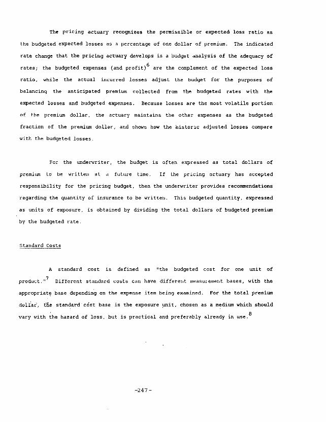
The pricing actuary recognizes the permissible or expected loss ratio as
the budgeted expected losses as a percentage of one dollar of premium. The indicated
rate change that the pricing actuary develops is a budget analysis of the adequacy of
rates; the budgeted expenses (and profit)6 are the complement of the expected loss
ratio, while the actual incurred losses adjust the budget for the purposes of
balancing the anticipated premium collected from the budgeted rates with the
expected losses and budgeted expenses. Because losses are the most volatile portion
of the premium dollar, the actuary maintains the other expenses as the budgeted
fraction of the premium dollar, and shows how the historic adjusted losses compare
with the budgeted losses.
For the underwriter, the budget is often expressed as total dollars of
premium to be written at a future time. If the pricing actuary has accepted
responsibility for the pricing budget, then the underwriter provides recommendations
regarding the quantity of insurance to be written. This budgeted quantity, expressed
as units of exposure, is obtained by dividing the total dollars of budgeted premium
by the budgeted rate.
Standard Costs
A standard cost is defined as "the budgeted cost for one unit of
product."7 Different standard costs can have different measurement bases, with the
appropriate base depending on the expense item being examined. For the total premium
dollar, flie standard cost base is the exposure unit, chosen as a medium which should
vary with the hazard of loss, but is practical and preferably already in use.’
-247-
The exposure unit, however, may not be the medium that varies most
directly with the level of expenses incurred. For example, a more appropriate
standard cost measure to analyze the budget variances for salary might be number of
hours worked rather than exposure units. Therefore, in the example shown in Appendix
B, hours worked is the salary standard cost base applied due to accuracy
considerations, although for practical purposes the exposure unit may be substituted.
Overhead Costs
Overhead costs, which are also known as indirect costs for an insurance
company, are all costs not directly associated with the selling costs of an
insurance product. Appendix A shows that overhead costs can be classified as
variable overhead costs, such as product promotion, underwriting, marketing or
actuarial, or fixed overhead costs, such as administration, marketing management,
and building and maintenance.
THE ANALYSIS OF BUDGET VARIANCES
With the cost accounting terminology introduced, the “Analysis of Budget
Variances" technique is presented.
Budget Variances--Variable Expenses
The total variance of actual results from expected results for variable
expenses can be divided into price and quantity variances. Although cost accounting
textbooks present this concept in terms of manufacturing companies, 9 this paper
adapts the technique for a service industry such as insurance. The following
-248-
example introduces an analysis method for the variable expenses through the loss
component, which is the most significant cost that varies directly with the earned
premium of an insurance company.
Example
Insurance Company Management (ICM) has outlined a Master Budget for the
year 1984. Based on discussions with the Underwriting Department, $1,400 of premium
is planned to be written on January 1, 1984. The Actuarial Department, basing its
recommendation on the rate indication, has budgeted a "standard price" for the rate
at $1.00 per exposure. The actuaries have also agreed that the standard cost for
losses, or expected loss ratio, for the 1,400 planned exposures ($1,400 : $1.00 per
exposure) is $.650, which will allow budgeted losses of $910.
After the close of the year, 1984 calendar year results show that 1,200
exposures were written at $.833 per exposure, for $1,000 of written and earned
premium. The incurred losses have been posted at $700 for the year. The results
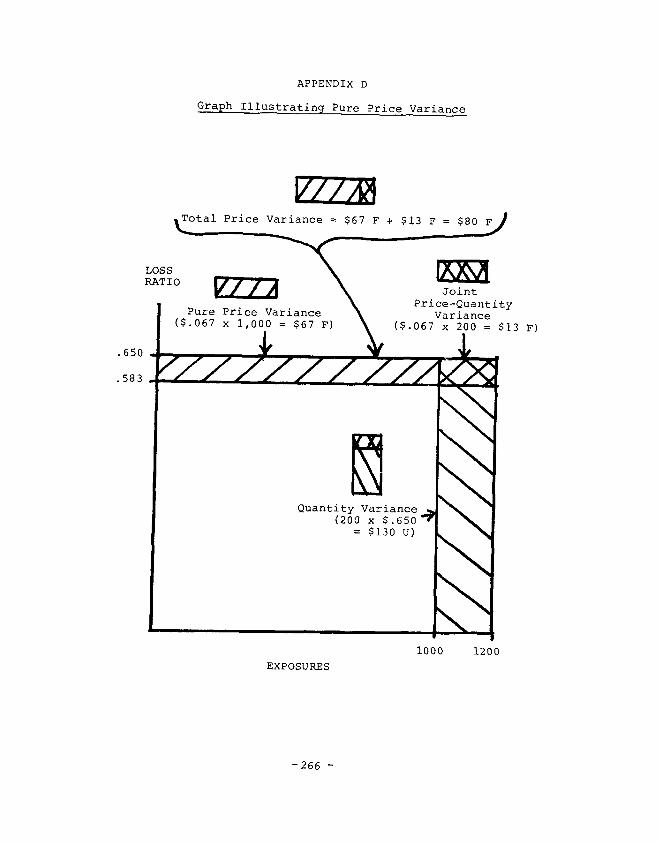
Joint Price-Quantity Pure Price Variance Variance=$li F -
Overall-Price Variance =$80 F
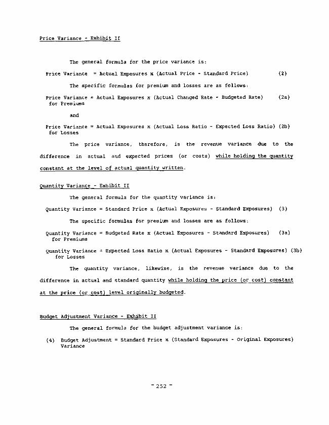
(2), is:
The general formula for the price variance, as stated in formula
Price Variance = Actual Exposures x (Actual Price - Standard Price) (2)
A pure price variance can be calculated as follows:
Pure Price Variance = Standard Exposures x (Actual Price - Standard Price) (7)
A joint price-quantity variance is defined as:
Joint Price-Quantity =
c
Actual Variance Exposures
(8)
The sum of formulas (7) and (8) equal the price variance,
formula (2), which is apparent from the formulas.
-256-
The pure price variance, therefore, is the revenue variance due to the
difference in actual and expected prices (or costs), while holding the quantity
constant at the level of expected quantity written. This variance is more pure
than the price variance, which holds the quantity at the level of actual quantity
written.
This additional procedure may be unnecessary, as the overall price
variance is a method of recognizing that the actual exposures written will impact
the price of a product through supply and demand elasticities.
The remaining specific formulas for premium and losses, which produce
Exhibit III, are as follows:
Pure Price Variance = Standard Exposures x for Premium I
Actual Charged Rate - Budgeted 3
(?a) Rate
Pure Price Variance = Standard Exposures x Actual Loss Ratio -
f
Expected 3
(7b) For Losses Loss Ratio
Joint Price-Quantity = I
Actual Exposures -
\t
x Actual Charged - Budgeted (8a) Variance for Premium Standard Exposures Rate Rate I
Joint Price-Quantity =
f
Actual Exposures - - Expected Loss 3
(8b) Variance for Losses Standard Exposures Ratio
Budget Variances--Fixed Expenses
The fixed costs are budgeted and monitored through a different analysis of
variance technique than the procedure described for the variable costs. The specific
technique, called fixed-overhead application, requires the development of a
fixed-overhead rate which will be used to monitor the fixed costs throughout the
budget period. This rate is computed by dividing the budgeted dollar level of fixed
costs by the best measure of capacity over the budget period. This measure is called
the denominator level. 11
-257 -
One insurance definition of capacity is "the total premium volume a single
multiple-line insurer can write for all lines of insurance." 12 As long as a
Kenney-type rule of the ratio of net written premium to policyholders' surplus is
followed, the choice for an appropriate denominator level is facilitated.
Example
1(31's master budget for 1984 includes $140 of fixed costs. Corporate
management has chosen to adhere to the Kenney rule, which states that capacity equals
twice the level of policyholders' surplus. 13 At December 31, 1983, policyholders'
surplus is $1,750, producing a denominator level of $3,500. The fixed overhead rate
is set at .04($140 : $3,500) per dollar of capacity.
On December 31, 1984, the net income statement shows $150 of fixed costs
were incurred, and $1,000 of premium was written. Exhibit IV shows the Fixed Costs
Analysis of Budget Variances.
-258 -
Exhibit IV Fixed Costs Analysis of Budget Variances
(1) (2) (3) Actual Fixed Flexible Budget Fixed Overhead Costs Incurred Based on Premium Applied
$150 $140 $100 (same regardless of volume level)
Spending Variance** Denominator Variance =$lO u =$40 u
Underapplied Overhead = $50 u
*Since $1,400 of premium was allowed in the master budget for $3,500 of capacity, then $1,000 of "good output" of premium actually written produces standard capacity of $2,500 (($1,000 : $1,400) x $3,500 = $2,500).
**The spending variance is the budget variance.
Uses of Fixed-Overhead Analysis
The fixed costs variance analysis does not have an explicit quantity
variance, as fixed costs are presumed to be constant over a range of volume levels.
Column (2) is called a flexible budget because the $140 was selected as the best
flexible measure of fixed costs over that range of volume levels.
The denominator variance, which replaces the quantity variance for fixed
costs analysis purposes, is an approximate measure of the efficiency of production.
This firm has been inefficient in its production, as the amount of premium actually
written is on the low end of the range of volume levels.
Wade warns that one of the potential misapplications of the contribution
method of allocation of expenses is in the treatment of the fixed costs. 14 The
contribution method is an appropriate technique to compare alternate policies in a
marginal situation only when fixed costs truly remain "fixed" over the analysis
period.
-259-
The spending variance, and the causes for its balance, should be examined
to discover the true reason for any observed changes in fixed costs. Although Wade
indicates that changes in the volume of business can affect the level of fixed costs,
other factors such as inflation or poor cost estimation methods can produce
unanticipated fixed cost differences.
Committed fixed costs, including depreciation, real estate taxes, and
insurance,15 are likely to be independent of short-term changes in volume. For
example, an unanticipated increase in property tax assessments could produce an
unfavorable spending variance, but would not likely be produced due to a change in
volume. Discretionary costs, which are budgeted fixed costs due to short-term
decisions, are more likely to be incurred due to growth reasons. Here, a recent
surge in premium writings might encourage a company to undertake a management
development program which it might not have afforded in the absence of the change in
volume.
These above examples illustrate that the contribution method of allocation
of expenses is not rendered an inappropriate comparison measure of alternatives, if
the fixed-overhead budget analysis reveals that the variances occurred for reasons
other than expanding capacity.
- 260-
This paper has presented a technique which can evaluate the variances of
the actual results from those expected for all the components of the net income
statement. Price and quantity variances, which can be produced for the premium and
variable cost components, may have some applications for the assignment of
responsibilty. The fixed costs analysis provides a more detailed evaluation of a
company's expense allocation system, which could be of value to the pricing actuary
as well as the corporate planning actuary.
-261-
APPENDIX A Net Income Statement Comparison 16
Full Absorption Method
Earned Premiums Incurred Losses Loss Adjustment Expenses Incurred Commissions Incurred Other Acquisition Expenses Incurred General Expenses Incurred Taxes, Licenses and Fees Incurred
Net Income
$100 s 30 $ 24
; 2: S 6
Contribution Method
Earned Premiums Loss and Loss Adjustment Expenses Incurred $130
(Variable Cost of Goods Sold) Variable Gross Profit
Commissions Incurred $ 24 Other Acquisition Expenses Incurred $ 28 Premium Taxes s 5 Other Variable Costs Associated with Product $ 2
(10% of General Expenses) Variable Profit (Distribution Contribution Margin)
Variable Overhead Expenses* $ 10 (50% of General Expenses)
Line of Business Contribution Margin Fixed Overhead Expenses** S 8
(40% of General Expenses) Other Taxes $1
Line of Business Profit/Net Income
$200
s 12
$200
$ 70
$ 31
$ 21
s 12
* Indirect Costs - Variable and Not Directly Associated with Product. ** Indirect Costs - Fixed and Not Directly Associated with Product.
-262 _
APPENDIX B
This Appendix contains examples of standard cost bases other than exposure
units to measure variable cost budget variances.
Examples--Hourly Wages and Number of Policies
A data processing department of an insurer has a clerical staff which is
paid an hourly wage. In order to monitor the budget for clerical salaries, a
standard cost system based on hourly wages is maintained.
This same insurer is also concerned with the General Expenses of the Other
Underwriting Expenses shown on Part 1 of the Investment Income Exhibit. In
particular, Items 3 through 17 are the itemized expenses to be monitored. All of
these expenses have been deemed variable overhead by this insurer. The clerical
salaries, to be examined in another standard cost base, are removed from these
expenses. The standard cost for this group of expenses is number of policies
written.
For 1984, the clerical salaries are budgeted for $100,000, composed of
20,000 hours at $5.00 per hour. The Other Underwriting Expenses are budgeted for
$150,000, with 500 policies planned at a cost of $300 per policy. Budgeted earned
premium for 1984 is $l,OOO,OOO.
Actual 1984 results show that 480 policies were written and $900,000 of
earned premium was posted. Union negotiations have raised the clerical hourly wage
to $5.20, and 17,000 hours have been worked by the clerical staff. The Other
Underwriting Expenses actually incurred total $139,200.
-263-
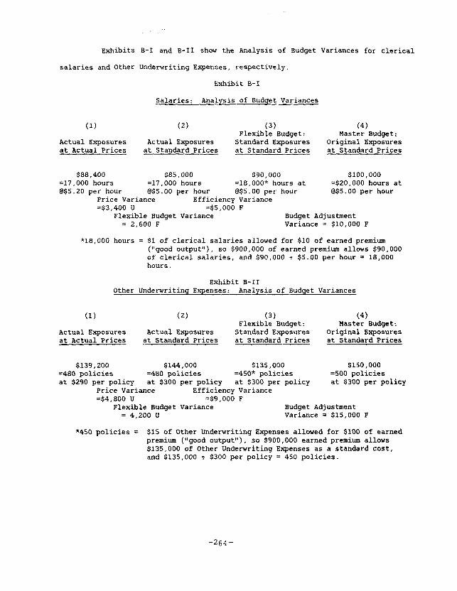
Exhibits B-I and B-II show the Analysis of Budget Variances for clerical
salaries and Other Underwriting Expenses, respectively.
Exhibit B-I
Salaries: Analysis of Budget Variances
(1) (2) (3) (4) Flexible Budget: Master Budget:
Actual Exposures Actual Exposures Standard Exposures Original Exposures at Actual Prices at Standard Prices at Standard Prices at Standard Prices
$88,400 $85,000 $90,000 =17,000 hours =17,000 hours =18,000* hours at @$5.20 per hour @$5.00 per hour @$5.00 per hour
Price Variance Efficiency Variance =$3,400 u =$5,000 F
$100,000 =$20,000 hours at @$5.00 per hour
Flexible Budget Variance = 2,600 F
Budget Adjustment Variance = $10,000 F
*18,000 hours = $1 of clerical salaries allowed for $10 of earned premium ("good output"), so $900,000 of earned premium allows $90,000 of clerical salaries, and $90,000 ‘r $5.00 per hour = 18,000 hours.
Exhibit B-II Other Underwriting Expenses: Analysis of Budget Variances
(1) (2) (3) (4) Flexible Budget: Master Budget:
Actual Exposures Actual Exposures Standard Exposures Original Exposures at Actual Prices at Standard Prices at Standard Prices at Standard Prices
$139,200 $144,000 $135,000 $150,000 =480 policies =480 policies =45O* policies =500 policies at $290 per policy at $300 per policy at $300 per policy at $300 per policy
Price Variance Efficiency Variance =$4,800 U =$9,000 F
Flexible Budget Variance Budget Adjustment = 4,200 U Variance = $15,000 F
"450 policies = $15 of Other Underwriting Expenses allowed for $100 of earned premium (“good output"), so $900,000 earned premium allows $135,000 of Other Underwriting Expenses as a standard cost, and $135,000 : $300 per policy = 450 policies.
-264-
LOSSES
800
600
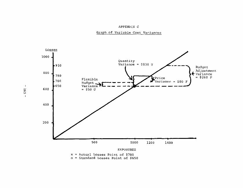
APPENDIX C
Graph of Variable Cost Variances
Quantity Variance = $130 U
/
a- --
'r Budget
. Adjustment 'Variance
'7kPrice \ = $260 F
200
EXPOSURES
x = Actual Losses Point of $700 o = Standard Losses Point of $650
APPENDIX D
Graph Illustrating Pure Price Variance
.650
.583
Quantity Variance \ (200 x $.650
= $130 U) +l \I
U
3 Fl
EXPOSURES
-266 -
1.
2.
3.
4.
5.
6.
7.
8.
9.
10.
11.
12.
13.
14.
15.
16.
FOOTNOTES
Charles T. Horngren, Cost Accounting: A Managerial Emphasis, 4th ed. (Englewood Cliffs, NJ: Prentice-Hall, Inc., 1977), p.4. Much of the general techniques for this paper are found in chapters 7 through 10 of this reference.
Roger C. Wade, "Expense Analysis in Ratemaking and Pricing," PCAS Vol. LX, 1973.
Ibid., p.1.
Ray H. Garrison, Managerial Accountinq, 3rd ed. (Plano, Texas: Business Publications, Inc., 1982), p. 288. Additional material for this paper, very similar to Horngren's, was gathered in chapters 8-10.
Ibid.
Explicit considerations for investment income and underwriting profit can embellish this method, but are ignored for the purposes of this paper.
Garrison, p-347.
Paul Dorweiler, 'lNotes on Exposures and Premium Bases," PCAS Vol. LVIII, 1971, p.60.
See Footnotes [l] and [4].
Wade, p.6.
Horngren, p.265
Robert I. Mehr, 'lInsurance Capacity: Issues and Perspectives," Issues in Insurance, Volume 1 (Malvern, PA: American Institute for Property and Liability Underwriters, 1981), p.318.