Neural Networks 19 (2006) 1047–1058www.elsevier.com/locate/neunet

2006 Special Issue

Building bridges between neural models and complex decisionmaking behaviour

Jerome R. Busemeyera,∗, Ryan K. Jessupa, Joseph G. Johnsonb, James T. Townsenda

a Department of Psychological and Brain Sciences, Indiana University, Bloomington, IN, USAb Department of Psychology, Miami University, Oxford, OH, USA

Received 11 January 2006; accepted 1 May 2006

Abstract

Diffusion processes, and their discrete time counterparts, random walk models, have demonstrated an ability to account for a wide range offindings from behavioural decision making for which the purely algebraic and deterministic models often used in economics and psychologycannot account. Recent studies that record neural activations in non-human primates during perceptual decision making tasks have revealed thatneural firing rates closely mimic the accumulation of preference theorized by behaviourally-derived diffusion models of decision making.

This article bridges the expanse between the neurophysiological and behavioural decision making literatures specifically, decision field theory[Busemeyer, J. R. & Townsend, J. T. (1993). Decision field theory: A dynamic-cognitive approach to decision making in an uncertain environment.Psychological Review, 100, 432–459], a dynamic and stochastic random walk theory of decision making, is presented as a model positionedbetween lower-level neural activation patterns and more complex notions of decision making found in psychology and economics. Potentialneural correlates of this model are proposed, and relevant competing models are also addressed.c© 2006 Elsevier Ltd. All rights reserved.

Keywords: Models, dynamic; Choice behaviours; Decision making; Basal ganglia; Neuroeconomics; Processes, diffusion/random walk

The decision processes of sensory-motor decisions arebeginning to be fairly well understood both at the behaviouraland neural levels. For the past ten years, neuroscientists havebeen using multiple cell recording techniques to examine spikeactivation patterns in rhesus monkeys during simple decisionmaking tasks (Britten, Shadlen, Newsome, & Movshon, 1993).In a typical experiment, the monkeys are presented with a visualmotion detection task which requires them to make a saccadiceye movement to a location indicated by a noisy visual display,and they are rewarded with juice for correct responses. Neuralactivity is recorded from either the middle temporal area (anextrastriate visual area), lateral intraparietal cortex (which playsa role in spatial attention), the frontal eye fields (FEF), orsuperior colliculus (SC, regions involved in the planning andimplementation of eye movements, respectively).

The typical findings indicate that neural activation regardingstimulus movement information is accumulated across time up

∗ Corresponding address: 1101 E. 10th Street, Bloomington, IN, 47405,USA. Tel.: +1 812 855 4882; fax: +1 812 855 4691.

E-mail address: jbusemey@indiana.edu (J.R. Busemeyer).

0893-6080/$ - see front matter c© 2006 Elsevier Ltd. All rights reserved.doi:10.1016/j.neunet.2006.05.043

to a threshold, and a behavioural response is made as soon as theactivation in the recorded area exceeds the threshold (see Goldand Shadlen (2000), Mazurek, Roitman, Ditterich, and Shadlen(2003), Ratcliff, Cherian, and Segraves (2003), Schall (2003),Shadlen and Newsome (2001) for examples). Because areassuch as FEF and SC are thought to implement the behaviourof interest (in this example, saccadic eye movements), aconclusion that one can draw from these results is that theneural areas responsible for planning or carrying out certainactions are also responsible for deciding the action to carry out,a decidedly embodied notion.

Mathematically, the spike activation pattern, as well as thechoice and response time distributions, can be well describedby what are known as diffusion models (see Smith and Ratcliff(2004) for a summary). Diffusion models can be viewed asstochastic recurrent neural network models, except that thedynamics are approximated by linear systems. The linearapproximation is important for maintaining a mathematicallytractable analysis of systems perturbed by noisy inputs. Inaddition to these neuroscience applications, diffusion models(or their discrete time, random walk, analogues) have been

1048 J.R. Busemeyer et al. / Neural Networks 19 (2006) 1047–1058

used by cognitive scientists to model performance in a varietyof tasks ranging from sensory detection (Smith, 1995), andperceptual discrimination (Laming, 1968; Link & Heath, 1975;Usher & McClelland, 2001), to memory recognition (Ratcliff,1978), and categorization (Ashby, 2000; Nosofsky & Palmeri,1997). Thus, diffusion models provide the potential to forma theoretical bridge between neural models of sensory-motortasks and behavioural models of complex-cognitive tasks.

The purpose of this article is to review applications ofdiffusion models to human decision making under risk withconflicting objectives. Traditionally, the field of decisionmaking has been guided by algebraic utility theories such as theclassic expected utility model (von Neumann & Morgenstern,1944) or more complex variants such as cumulative prospecttheory (Tversky & Kahneman, 1992). However, a numberof paradoxical findings have emerged in the field of humandecision making that are difficult to explain by traditionalutility theories. We show that diffusion models provide a cogentexplanation for these complex and puzzling behaviours. First,we describe how diffusion models can be applied to riskydecisions with conflicting objectives; second, we explain someimportant findings using this theory; and finally, we comparethis theory with some alternate competing neural networkmodels.

1. Risky decisions with multiple objectives

Consider the following type of risky decision with multipleobjectives. Suppose a commander is suddenly confronted byan emergency situation, and must quickly choose one actionfrom a set of J actions, labelled here as A1, . . . , A j , . . . , AJ .The payoff for each action depends on one of set of Kuncertain states of the world X1, . . . , Xk, . . . , X K . Thepayoff produced by taking action j under state of the world k isdenoted x jk . Finally, each payoff can be described in terms ofmultiple competing objectives (e.g. one objective is to achievethe commander’s mission while another objective is to preservethe commander’s resources).

According to the ‘rational’ model (Savage, 1954; vonNeumann & Morgenstern, 1944), the decision maker shouldchoose the course of action that maximizes expected utility:EU (A j ) =

∑k pk · u(x jk), where pk is the probability

of state Xk and u(x jk) is the utility of payoff x jk .Psychological variants of expected utility theory modify theclassic model by replacing the objective probabilities withsubjective decision weights (e.g. Birnbaum, Coffey, Mellers,and Weiss (1992), Tversky and Kahneman (1992)).

2. Decision field theory

An alternate approach towards explaining risky choicebehaviour involves the application of diffusion processes, viadecision field theory. We have applied diffusion models toa broad range of results including findings from decisionmaking under uncertainty (Busemeyer & Townsend, 1993),multi-attribute decisions (Diederich, 1997), multi-alternativechoices (Roe, Busemeyer, & Townsend, 2001) and multiple

measures of preference (Johnson & Busemeyer, 2005). Thebasic assumptions of the model are summarized below.

2.1. Basic assumptions

Define P(t) as a J dimensional preference state vector,and each coordinate, Pj (t), represents the preference statefor one of the J actions under consideration. The preferencestates may range from positive (approach states) to negative(avoidance states), and the magnitude of a preference staterepresents the strength of the approach–avoidance tendency.The initial state at the beginning of the decision process, P(0),represents preferences before any information about the actionsis considered, such as memory from previous experience witha decision problem (

∑j Pj (0) = 0). For novel decisions, the

initial states are all set equal to zero (neutral), Pj (0) = 0 forall j . The change in state across a small time increment h isdenoted by d P(t) = P(t) − P(t − h).

During deliberation the preference state vector evolvesaccording to the following linear stochastic difference equation(t = n · h and n = 1, 2, . . .)

d P(t) = −h · 0 · P(t − h) + V (t) (1a)

or equivalently

P(t) = (I − h · 0) · P(t − h) + V (t)

= S · P(t − h) + V (t) (1b)

where S = (I − h · 0) is a J × J feedback matrix, V (t) is a Jdimensional stochastic input, and I is the identity matrix. Thesolution to this linear stochastic difference equation equals

P(t) =

n−1∑τ=0

Sτ V (t − τh) + Sn P(0). (2)

As h → 0, this system approximates an Ornstein–Uhlenbeckdiffusion process (see Busemeyer and Diederich (2002), Buse-meyer and Townsend (1992)). If the feedback matrix is set toS = I (i.e. 0 = 0), then the Ornstein–Uhlenbeck model re-duces to a Wiener diffusion process.

The feedback matrix 0 contains self feedback coefficients,γi i = γ are all equal across the diagonals, as well assymmetrical lateral inhibitory connections γi j = γ j i . Themagnitudes of the lateral inhibitory connections are assumedto be inversely related to the conceptual distance between theactions (examples are discussed later). The preference statevector, P(t), remains bounded as long as the eigenvalues of Sare less than one in magnitude. Lateral inhibition is commonlyused in competitive neural network systems (Grossberg, 1988;Rumelhart & McClelland, 1986).

The stochastic input vector, V (t), is called the valence, andeach coordinate, V j (t), represents avoidance (when activationsare negative) or approach (when activations are positive) forceson the preference state for the j th action. The valence vector isdecomposed into three parts as follows:

V (t) = C · M · W (t), (3)

J.R. Busemeyer et al. / Neural Networks 19 (2006) 1047–1058 1049

where C is a J × J contrast matrix, M is a J × K value matrix,and W (t) is a K × 1 stochastic attention weight vector. Eachelement, m jk , of the value matrix M represents the affectiveevaluation of each possible consequence k for each action j .The product of the stochastic attention weight vector with thevalue matrix, M ·W (t), produces a weighted average evaluationfor each action at any particular moment. The contrast matrix Chas elements ci j = 1 for i = j and ci j = −1/(J −1) for i 6= j ,which are designed to compute the advantage or disadvantageof each action relative to the average of the other actions at eachmoment. (Note that

∑j ci j = 0 implies that

∑V j (t) = 0.)

The weight vector, W (t), is assumed to fluctuate frommoment to moment, representing changes in attention to theuncertain states across time. More formally, the attentionweights are assumed to vary according to a stationary stochasticprocess with mean E[W (t)] = w · h, and variance–covariancematrix Cov[W (t)] = Ψ · h.1The mean weight vector, w, is aK × 1 vector, and each coordinate, wk = E[Wk(t)], representsthe average proportion of time spent attending to a particularstate, Xk , with k ∈ 1, . . . , K .

2.2. Derivations

These assumptions lead to the following implications. Themean input valence equals E[V (t)] = δ · h = (C · M · w) · h,and the variance–covariance matrix of the input valence equalsCov[V (t)] = Φ · h = (CMΨM′C′) · h. The mean preferencestate vector equals

ξ(t) = E[P(t)] =

n−1∑τ=0

Sτ δ · h + Sn P(0)

= (I − S)−1(I − Sn) · δ · h + Sn P(0). (4)

As t → ∞, ξ(∞) = (I − S)−1· δ · h so that the mean

preference state is a linear transformation of the mean valence.The variance–covariance of the preference state vector equals

Ω(t) = Cov[P(t)] = h ·

n−1∑τ=0

SτΦ(Sτ )′. (5)

For the special case where Φ = φ2· I, then Ω(t) = h ·φ2

· (I −

S2)−1(I−S2n); and as t → ∞, then Ω(∞) = h ·φ2·(I−S2)−1.

Finally, if it is assumed that the attention weights changeacross time according to an independent and identicallydistributed process, then it follows from the central limittheorem that the distribution for the preference state vectorwill converge in time to a multivariate normal distribution withmean ξ(t) and covariance matrix Ω(t). The derivation for thechoice probabilities depends on the assumed stopping rule forcontrolling the decision time, which is described next.

1 Preference is a stochastic process which should converge to a diffusionprocess as h → 0. The properties of preference depend upon the valence whichis a random variable because the attention weights are random. In order forpreference to converge to a diffusion process, the mean and variance must beproportional to h. And because valence is a linear transformation of the weights,the mean and variance of the weight vector must be proportional to h.

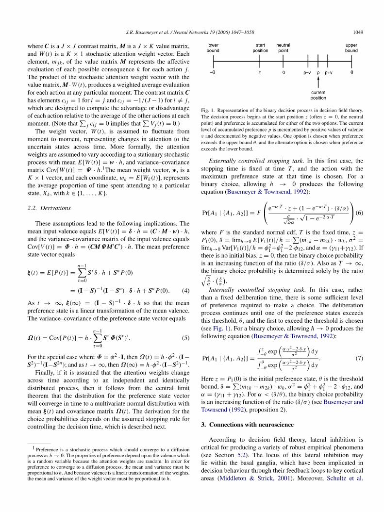
Fig. 1. Representation of the binary decision process in decision field theory.The decision process begins at the start position z (often z = 0, the neutralpoint) and preference is accumulated for either of the two options. The currentlevel of accumulated preference p is incremented by positive values of valencev and decremented by negative values. One option is chosen when preferenceexceeds the upper bound θ , and the alternate option is chosen when preferenceexceeds the lower bound.

Externally controlled stopping task. In this first case, thestopping time is fixed at time T , and the action with themaximum preference state at that time is chosen. For abinary choice, allowing h → 0 produces the followingequation (Busemeyer & Townsend, 1992):

Pr[A1 | A1, A2] = F

e−α·T· z + (1 − e−α·T ) · (δ/α)

σ√

2·α·√

1 − e−2·α·T

(6)

where F is the standard normal cdf, T is the fixed time, z =

P1(0), δ = limh→0 E[V1(t)]/h =∑

(m1k − m2k) · wk , σ 2=

limh→0 Var[V1(t)]/h = φ21+φ2

1−2·φ12, and α = (γ11+γ12). Ifthere is no initial bias, z = 0, then the binary choice probabilityis an increasing function of the ratio (δ/σ ). Also as T → ∞,the binary choice probability is determined solely by the ratio√

2α

·(

δσ

).

Internally controlled stopping task. In this case, ratherthan a fixed deliberation time, there is some sufficient levelof preference required to make a choice. The deliberationprocess continues until one of the preference states exceedsthis threshold, θ , and the first to exceed the threshold is chosen(see Fig. 1). For a binary choice, allowing h → 0 produces thefollowing equation (Busemeyer & Townsend, 1992):

Pr[A1 | A1, A2] =

∫ z−θ

exp(

α·y2−2·δ·yσ 2

)dy∫ θ

−θexp

(α·y2−2·δ·y

σ 2

)dy

. (7)

Here z = P1(0) is the initial preference state, θ is the thresholdbound, δ =

∑(m1k − m2k) · wk , σ 2

= φ21 + φ2

1 − 2 · φ12, andα = (γ11 + γ12). For α < (δ/θ), the binary choice probabilityis an increasing function of the ratio (δ/σ ) (see Busemeyer andTownsend (1992), proposition 2).

3. Connections with neuroscience

According to decision field theory, lateral inhibition iscritical for producing a variety of robust empirical phenomena(see Section 5.2). The locus of this lateral inhibition maylie within the basal ganglia, which have been implicated indecision behaviour through their feedback loops to key corticalareas (Middleton & Strick, 2001). Moreover, Schultz et al.

1050 J.R. Busemeyer et al. / Neural Networks 19 (2006) 1047–1058

(1995) observed that dopaminergic neurons afferent to thebasal ganglia fire in concert with reliable predictors of reward(see also Gold (2003), Hollerman and Schultz (1998), andSchultz (1998, 2002)). Together these findings support thenotion that the basal ganglia have an important function indecision behaviour.

Knowledge of the basal ganglia architecture should enhanceour understanding of the role of lateral inhibition withincortico-striatal loops. In particular, we are concerned with twosubstructures in the basal ganglia, the globus pallidus internalsegment (GPi) and the striatum. Within the cortico-striatalloops, axons from the cortex enter into the basal ganglia viathe striatum, which then projects to GPi, which in turn projectsto the thalamus which sends afferent connections to the corticalarea from which it arose, creating a looped circuit of neuralcommunication (Middleton & Strick, 2001).

The striatum consists of approximately 95% GABAergicmedium spiny neurons (Gerfen & Wilson, 1996). BecauseGABA is an inhibitory neurotransmitter, these are inhibitoryneurons. Additionally, these striatal neurons have extensivelocal arborization of dendrites and axons, creating a networkof distance dependent laterally inhibited neurons (Wickens,1997; Wilson & Groves, 1980). Striatal neurons have inhibitoryconnections to GPi, the output mechanism of the basal gangliacomplex. GPi consists of tonically active neurons (TANs),which exert their effects by continuously firing, so as torelentlessly inhibit post-synaptic neurons in the thalamus; onlyby inhibition of inhibitory neurons can neurons cast off theshackles of TANs. Inhibition of GPi by striatal neurons releasesthe thalamus to signal the frontal cortex to engage in the actionpreferred by striatal neurons. This process is known as thalamicdisinhibition.

Naturally, when one option appears in isolation, the lackof lateral inhibition from competing alternatives will enableit to quickly inhibit corresponding GPi neurons2; however,multiple competing alternatives arouse lateral inhibition. Muchas the edge detectors in the bipolar cells within the retina(which also employ distance dependent lateral inhibition) aretuned to contrasts and thereby enhance differences, these basalganglia cells can also be thought of as focusing on contrastsbetween alternatives. Thus, the local contrasts between adominated alternative are effectively magnified by striatal units,giving more proximal alternatives an advantage over moredistal options where contrasts are less magnified. The negatedinhibition employed by decision field theory appears to mimicthis magnification of local differences.

On the other hand, it might be reasonable to suggest that thenegated inhibition corresponds with thalamic disinhibition, orstriatal inhibition of GPi (see Busemeyer, Townsend, Diederich,and Barkan (2005), Vickers and Lee (1998) for relatedproposals). While distributed representations of alternatives

2 It is important to note that rarely are we faced with one option in isolation,as we can seemingly always choose the ‘not’ option, i.e. we can choose to buyor to not buy; the notion of ‘one option’ is rather artificial. An alternate construalmight arise when the option to choose dominates the ‘not’ option; this may bewhat is generally implied when it is said that there is only one option.

via striatal neurons engage in lateral inhibition, they alsosend inhibitory connections to tonically active GPi neurons.As information favouring one alternative begins to weaken,representative neurons send less lateral and pallidal (i.e. tothe GPi) inhibition. Competitive striatal neurons representingalternate options are thus less inhibited, enabling them toincrease inhibition of both the weakened alternative and GPineurons representing their specific alternative. This might lookvery much like the negated inhibition employed by decisionfield theory.

4. The bridge

Decision field theory is based on essentially the sameprinciples as the neural models of sensory-motor decisions(e.g. Gold and Shadlen (2001, 2002)—preferences accumulateover time according to a diffusion process. So how does thiskind of model relate to expected utility models? To answerthis question, it is informative to take a closer look at a simpleversion of the binary choice model in which S = I (i.e. 0 = 0).In this case:

P1(t) = P1(t − h) + V1(t) = z +

n−1∑τ=1

V1(τ · h) (8)

where z = P1(0). Recall that E[V (t)] = h ·C·M ·w = h ·δ, and

for J = 2 alternatives, C =

[1 −1−1 1

]and δ =

[δ1δ2

]=

[δ

−δ

]. The

expectation for the first coordinate equals:

E[V1(t)] = δ · h =

(∑wk · m1k −

∑wk · m2k

)· h

= (µ1 − µ2) · h (9)

where wk = E[Wk(t)] is the mean attention weightcorresponding to the state probability, pk , in the classicexpected utility model, µ j =

∑wk · m jk corresponding to

the expected utility of the j th option, and right hand side ofEq. (9) corresponds to a difference in expected utility. Thus thestochastic element, V1(t), can be broken down into two parts: itsexpectation plus its stochastic residual, with the latter definedas ε(t) = V1(t) − δ · h. Inserting these definitions into Eq. (8)produces

P1(t) = (µ1 − µ2) · t +

(z +

n−1∑τ=1

ε(τ · h)

). (10)

According to Eq. (10), the preference state is linearly related tothe mean difference in expected utilities plus a noise term.

By comparing Eqs. (8) and (10), one can see that itis clearly unnecessary to assume that the neural systemactually computes a sum of the products of probabilities andutilities so as to compute expected utility when choosingbetween alternatives; instead, an expected utility estimatesimply emerges from temporal integration. According to thisanalysis, neuroeconomists should not be looking for locationsin the brain that combine probabilities with utilities. The keyquestion to ask is what neural circuit in the brain carries outthis temporal integration.

J.R. Busemeyer et al. / Neural Networks 19 (2006) 1047–1058 1051

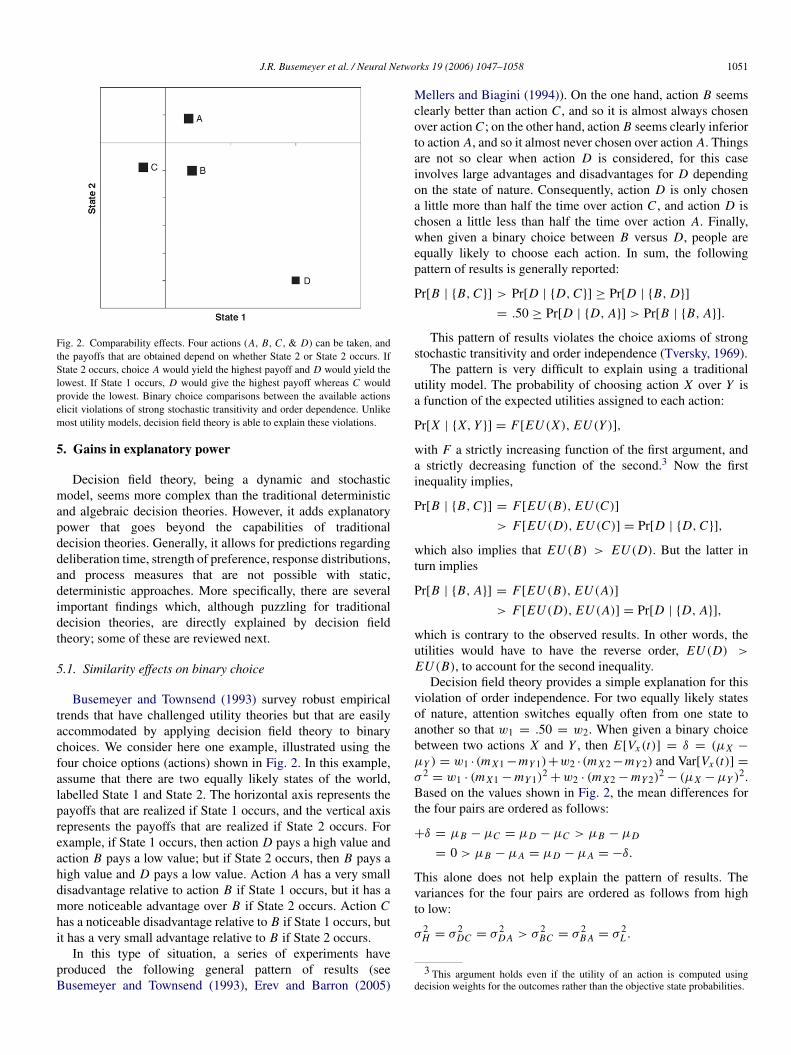
Fig. 2. Comparability effects. Four actions (A, B, C , & D) can be taken, andthe payoffs that are obtained depend on whether State 2 or State 2 occurs. IfState 2 occurs, choice A would yield the highest payoff and D would yield thelowest. If State 1 occurs, D would give the highest payoff whereas C wouldprovide the lowest. Binary choice comparisons between the available actionselicit violations of strong stochastic transitivity and order dependence. Unlikemost utility models, decision field theory is able to explain these violations.

5. Gains in explanatory power

Decision field theory, being a dynamic and stochasticmodel, seems more complex than the traditional deterministicand algebraic decision theories. However, it adds explanatorypower that goes beyond the capabilities of traditionaldecision theories. Generally, it allows for predictions regardingdeliberation time, strength of preference, response distributions,and process measures that are not possible with static,deterministic approaches. More specifically, there are severalimportant findings which, although puzzling for traditionaldecision theories, are directly explained by decision fieldtheory; some of these are reviewed next.

5.1. Similarity effects on binary choice

Busemeyer and Townsend (1993) survey robust empiricaltrends that have challenged utility theories but that are easilyaccommodated by applying decision field theory to binarychoices. We consider here one example, illustrated using thefour choice options (actions) shown in Fig. 2. In this example,assume that there are two equally likely states of the world,labelled State 1 and State 2. The horizontal axis represents thepayoffs that are realized if State 1 occurs, and the vertical axisrepresents the payoffs that are realized if State 2 occurs. Forexample, if State 1 occurs, then action D pays a high value andaction B pays a low value; but if State 2 occurs, then B pays ahigh value and D pays a low value. Action A has a very smalldisadvantage relative to action B if State 1 occurs, but it has amore noticeable advantage over B if State 2 occurs. Action Chas a noticeable disadvantage relative to B if State 1 occurs, butit has a very small advantage relative to B if State 2 occurs.

In this type of situation, a series of experiments haveproduced the following general pattern of results (seeBusemeyer and Townsend (1993), Erev and Barron (2005)

Mellers and Biagini (1994)). On the one hand, action B seemsclearly better than action C , and so it is almost always chosenover action C ; on the other hand, action B seems clearly inferiorto action A, and so it almost never chosen over action A. Thingsare not so clear when action D is considered, for this caseinvolves large advantages and disadvantages for D dependingon the state of nature. Consequently, action D is only chosena little more than half the time over action C , and action D ischosen a little less than half the time over action A. Finally,when given a binary choice between B versus D, people areequally likely to choose each action. In sum, the followingpattern of results is generally reported:

Pr[B | B, C] > Pr[D | D, C] ≥ Pr[D | B, D]

= .50 ≥ Pr[D | D, A] > Pr[B | B, A].

This pattern of results violates the choice axioms of strongstochastic transitivity and order independence (Tversky, 1969).

The pattern is very difficult to explain using a traditionalutility model. The probability of choosing action X over Y isa function of the expected utilities assigned to each action:

Pr[X | X, Y ] = F[EU (X), EU (Y )],

with F a strictly increasing function of the first argument, anda strictly decreasing function of the second.3 Now the firstinequality implies,

Pr[B | B, C] = F[EU (B), EU (C)]

> F[EU (D), EU (C)] = Pr[D | D, C],

which also implies that EU (B) > EU (D). But the latter inturn implies

Pr[B | B, A] = F[EU (B), EU (A)]

> F[EU (D), EU (A)] = Pr[D | D, A],

which is contrary to the observed results. In other words, theutilities would have to have the reverse order, EU (D) >

EU (B), to account for the second inequality.Decision field theory provides a simple explanation for this

violation of order independence. For two equally likely statesof nature, attention switches equally often from one state toanother so that w1 = .50 = w2. When given a binary choicebetween two actions X and Y , then E[Vx (t)] = δ = (µX −

µY ) = w1 · (m X1 −mY 1)+w2 · (m X2 −mY 2) and Var[Vx (t)] =

σ 2= w1 · (m X1 − mY 1)

2+ w2 · (m X2 − mY 2)

2− (µX − µY )2.

Based on the values shown in Fig. 2, the mean differences forthe four pairs are ordered as follows:

+δ = µB − µC = µD − µC > µB − µD

= 0 > µB − µA = µD − µA = −δ.

This alone does not help explain the pattern of results. Thevariances for the four pairs are ordered as follows from highto low:

σ 2H = σ 2

DC = σ 2D A > σ 2

BC = σ 2B A = σ 2

L .

3 This argument holds even if the utility of an action is computed usingdecision weights for the outcomes rather than the objective state probabilities.

1052 J.R. Busemeyer et al. / Neural Networks 19 (2006) 1047–1058

By itself, this also does not explain the pattern. The key pointis that the binary choice probability is an increasing function ofthe ratio (δ/σ ), and the ratios reproduce the correct order:

(µB − µC )/σBC = +δ/σL > (µD − µC )/σDC

= +δ/σH > (µD − µB)/σDB

= 0/σL > (µD − µA)/σD A = −δ/σH

> (µB − µA)/σB A = −δ/σL .

In sum, including action D in a pairwise choice produces ahigher variance, making it hard to discriminate the differences;whereas including option B produces a lower variance, makingit easy to discriminate the differences. In this way, decision fieldtheory provides a simple explanation for a result that is difficultto explain by a utility model.

5.2. Context effects on multi-alternative choice

Whereas Busemeyer and Townsend (1993) apply decisionfield theory to binary choice situations such as in the previoussection, Roe et al. (2001) show how the same theory canaccount for decisions involving multiple alternatives. Choicebehaviour becomes even more perplexing when there are morethan two options in the choice set. A series of experiments haveshown the preference relation between two of the options, sayA and B, can be manipulated by the context provided by addinga third option to the choice set (see Rieskamp, Busemeyer, andMellers (2006), Roe et al. (2001), Wedell (1991)).

The reference point effect (Tversky and Kahneman (1992));see also Wedell (1991) provides a compelling example. Thebasic ideas are illustrated in Fig. 3, where each letter shownin the figure represents a choice option described by twoconflicting objectives. In this case, option A is very good onthe first objective but poor on the second, whereas option B ispoor on the first objective and high on the second. When givena binary choice between options A versus B, people tend to beequally likely to choose either option. (Ignore option C for thetime being).

Option Ra has a small advantage over A on the seconddimension, but a more noticeable disadvantage on the firstdimension. Thus Ra is relatively unattractive compared tooption A. Similarly, option Rb has a small advantage over Bon the first dimension but a more noticeable disadvantage onthe second dimension. Thus option Rb is relatively unattractivecompared to option B.

For the critical condition, individuals are presented withthree options: A, B, and a third option, R, which is used tomanipulate a reference point. Under one condition, participantsare asked to assume that the current option Ra is the status quo(reference point), and they are then given a choice of keepingRa or exchanging this position for either action A or B. Underthese conditions, Ra was rarely chosen, and A was favouredover B. Under a second condition, participants are asked toimagine that option Rb is the status quo, and they are then givena choice of keeping Rb or exchanging this position for either Aor B. Under this condition, Rb was rarely chosen again, but nowB was favoured over A. Thus the preference relation between A

Fig. 3. Context effects can impact decisions. Option A is high on Dimension1 but low on Dimension 2 whereas B is high on Dimension 2 but low onDimension 1. Option C can be thought of as a compromise, and options Raand Rb can be used as reference points. Although preference for options Aand B are equivalent in binary choice comparisons, preference for A increaseswhen Ra is present; likewise, preference for B increases when the choice setincludes A, B, and Rb . This violation of regularity cannot be explained byheuristic models of choice. When presented with binary comparisons involvingtwo of A, B, and C , preference for each option is equal. However, when allthree options are simultaneously available, option C emerges as a preferredalternative, an effect which neither heuristic choice nor classic utility modelscan easily explain. Decision field theory can explain each of these effectswithout even adjusting its parameters across the conditions (see Roe et al.(2001) for other related findings).

and B reverses depending on whether the choice is made withrespect to the context provided by the reference point Ra or Rb.

In sum, the following pattern of choice probabilities isgenerally found (Tversky and Kahneman (1992); see alsoWedell (1991)):

Pr[A | A, B, Ra] > Pr[A | A, B]

= .50 > Pr[B | A, B, Ra],

Pr[B | A, B, RB] > Pr[B | A, B]

= .50 > Pr[A | A, B, Rb].

According to a traditional utility model, it seems as if option Ais equal in utility to option B under binary choice, but option Ahas greater utility than B from the Ra point of view, and optionB has greater utility than A from the Rb point of view.

There is a second and equally important qualitative findingthat occurs with this choice paradigm, which is called theattraction effect (Heath & Chatterjee, 1995; Huber & Puto,1983; Huber, Payne, & Puto, 1982; Simonson, 1989). Notethat the choice probability from a set of three options exceedsthat for the subset: Pr[A | A, B, Ra] > Pr[A | A, B]. Itseems that adding the deficient option Ra makes option A lookbetter than it appears within the binary choice context. This is aviolation of an axiom of choice called the regularity principle.Violations of regularity cannot be explained by heuristic choicemodels such as Tversky’s (1972) elimination by aspects model(see Rieskamp et al. (2006), Roe et al. (2001)).

Decision field theory explains these effects through thelateral inhibition mechanism in the feedback matrix S. Consider

J.R. Busemeyer et al. / Neural Networks 19 (2006) 1047–1058 1053

(I − S2)−1=

1

det[I − S2]·

1 + s4− b2(3 − 2b2) − s2(b2

+ 2) b2(1 + 3s2− 2b2) −2sb · (1 − s2)

b2(1 + 3s2− 2b2) 1 + s2

− b2(3 − 2b2) − s2(b2+ 2) −2sb · (1 − s2)

−2sb · (1 − s2) −2sb · (1 − s2) (1 − s2)(1 − s2− 2b2)

Box I.

first a choice among options A, B, Ra. In this case, B isvery dissimilar to both A and Ra and so the lateral inhibitionconnection between these two is very low (say zero forsimplicity); yet A is very similar to Ra and so the lateralinhibition connection between these two is higher (b > 0).Allowing rows 1, 2, and 3 to correspond to options A, B, Rarespectively, then the feedback matrix can be represented as

S =

s 0 −b0 s 0−b 0 s

.

The eigenvalues of S in this case are (s, s −b, s +b), which arerequired to be less than unity to maintain stability. In addition,to account for the binary choices, we set µA = µB = µ, andµR = −2µ, so that A and B have equal weighted mean values,and option Ra is clearly inferior. Note that A and B are equallylikely to be chosen in a binary choice, but this no longer followsin the triadic choice context. For in the latter case, we find thatthe mean preference state vector converges asymptotically to:

ξ(∞) = h · (I − S)−1µ

= h ·

(1 − s + 2b)µ

(1 − s − b)(1 − s + b)µ

1 − s(−2 + 2s − b)µ

(1 − s − b)(1 − s + b)

. (11)

The asymptotic difference between the mean preference statesfor A and B are obtained by subtracting the first two rows,which yields:

ξA − ξB = h ·µ · b(2(1 − s) + b)

(1 − s)(1 − s − b)(1 − s + b). (12)

This difference must be positive, producing a choice probabilitythat favours A over B. As µ increases, the probability ofchoosing option Ra goes to zero, while the difference betweenoptions A and B increases, which drives the probability ofchoosing option A toward 1.0.

If the reference point is changed from option Ra to optionRb, then the roles of A and B reverse. The same reasoningnow applies, and the sign of the difference shown in Eq. (12)reverses. Thus, if the reference point is changed to option Rb,then option B is chosen more frequently than A, producing apreference reversal. In sum, decision field theory predicts thatboth reference point and attraction effects result from changesin the mean preference state generated by the lateral inhibitoryconnections (see Busemeyer and Johnson (2004), Roe et al.(2001) for more details.)

Another important example of context effects is thecompromise effect, which involves option C in Fig. 3.

When given a binary choice between options A versus B,people are equally likely to choose either option. The sameholds for binary choices between options A versus C , andbetween B versus C . However, when given a choice amongall three options, then option C becomes the most popularchoice (Simonson, 1989; Tversky & Simonson, 1993). Withinthe triadic choice context, option C appears to be a goodcompromise between the two extremes.

The compromise effect poses problems for both traditionalutility models as well as simple heuristic choice models.According to a utility model, the binary choice results implyequal utility for each of the three options; but the triadic choiceresults imply a greater utility for the compromise. Accordingto a heuristic rule, such as the elimination by aspects rules ora lexicographic rule, the intermediate option should never bechosen, and only one of the extreme options should be chosen.

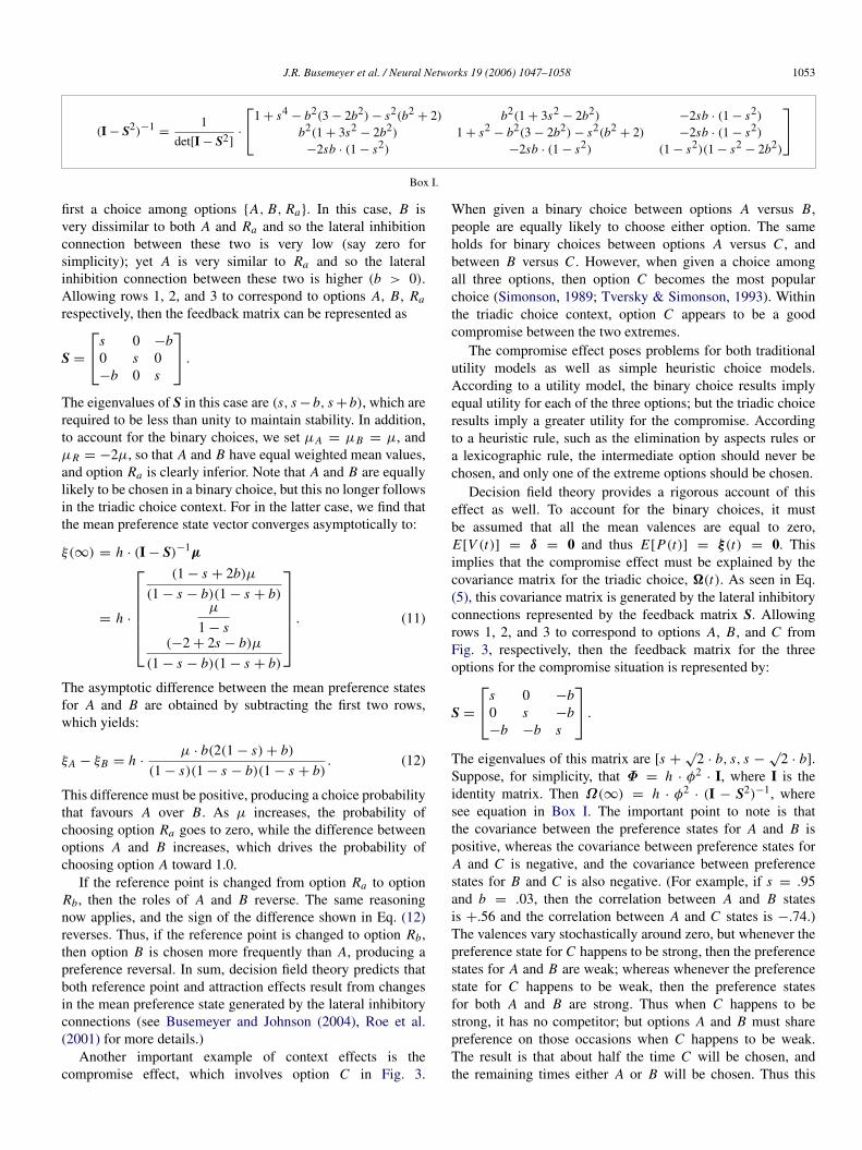
Decision field theory provides a rigorous account of thiseffect as well. To account for the binary choices, it mustbe assumed that all the mean valences are equal to zero,E[V (t)] = δ = 0 and thus E[P(t)] = ξ(t) = 0. Thisimplies that the compromise effect must be explained by thecovariance matrix for the triadic choice, (t). As seen in Eq.(5), this covariance matrix is generated by the lateral inhibitoryconnections represented by the feedback matrix S. Allowingrows 1, 2, and 3 to correspond to options A, B, and C fromFig. 3, respectively, then the feedback matrix for the threeoptions for the compromise situation is represented by:

S =

s 0 −b0 s −b−b −b s

.

The eigenvalues of this matrix are [s +√

2 · b, s, s −√

2 · b].Suppose, for simplicity, that Φ = h · φ2

· I, where I is theidentity matrix. Then Ω(∞) = h · φ2

· (I − S2)−1, wheresee equation in Box I. The important point to note is thatthe covariance between the preference states for A and B ispositive, whereas the covariance between preference states forA and C is negative, and the covariance between preferencestates for B and C is also negative. (For example, if s = .95and b = .03, then the correlation between A and B statesis +.56 and the correlation between A and C states is −.74.)The valences vary stochastically around zero, but whenever thepreference state for C happens to be strong, then the preferencestates for A and B are weak; whereas whenever the preferencestate for C happens to be weak, then the preference statesfor both A and B are strong. Thus when C happens to bestrong, it has no competitor; but options A and B must sharepreference on those occasions when C happens to be weak.The result is that about half the time C will be chosen, andthe remaining times either A or B will be chosen. Thus this

1054 J.R. Busemeyer et al. / Neural Networks 19 (2006) 1047–1058

Fig. 4. Equal density contours for computing triadic choice probabilities. Theleftmost panel demonstrates the contour for the density function of option A,where positive values on the horizontal axis indicate preference for option Aover option C and positive values on the vertical axis indicate preference foroption A over B. There is a +.22 correlation in the left panel for a choice ofA, and the same is true for the middle panel (preference for B), but there isa +.93 correlation shown in the right panel for the choice of C . This figuredemonstrates that when option C is preferred to option A, it is also very likelyto be preferred to option B, allowing it to obtain an inordinately large share ofpreference, whereas preference for A over C does not indicate that it will bepreferred over option B.

covariance structure provides option C with an advantage overA and B.

Fig. 4 illustrates the effect of the covariance structure on theasymptotic distribution of the differences in preference states(with s = .95 and b = .03). The panel on the left showsthe equal density contours for [PA(∞) − PC (∞), PA(∞) −

PB(∞)]: the probability that the preference state for A exceedsthat for both B and C is the integral over the positive righthand quadrant in this figure, which equals .29. The middlepanel illustrates the equal density contours for [PB(∞) −

PC (∞), PB(∞) − PA(∞)]: the probability that the preferencestate for B exceeds that for A and C is again .29. Finally, theright panel shows the equal density contours for [PC (∞) −

PB(∞), PC (∞) − PA(∞)]: the probability that the preferencestate for C exceeds that for A and B equals .43. In sum,decision field theory predicts the compromise effect as a resultof the covariance structure generated by the lateral inhibitoryconnections (see Roe et al. (2001), for more details).

5.3. Deliberation time effects on choice

Decisions take time, and the amount of time allocatedto making a decision can change preferences. Decision fieldtheory has been successful in accounting for a number offindings concerning the effects of deliberation time on choiceprobability (see Busemeyer (1985), Diederich (2003), Dror,Busemeyer, and Basola (1999)). Busemeyer and Townsend(1993) discuss the ability of decision field theory to accountfor speed–accuracy tradeoffs that are evident in many choice

Fig. 5. Predictions for the attraction effect as a function of deliberationtime. P A2 and P B2 indicate choice probability as a function of deliberationtime for options A and B, respectively (from Fig. 3), in the binary choicecondition whereas P A3 and P B3 demonstrate preference for Options A andB, respectively, during triadic choice when option Ra is included in the choiceset. Decision field theory predicts that the attraction effect should increasewith deliberation time, an effect empirically demonstrated Dhar et al., 2000;Simonson, 1989.

situations. That is, in general, choice probabilities aremoderated with decreases in deliberation time.

As an example, consider once again the attraction effectreferred to in Fig. 3: Adding a third option Ra to the choiceset increases the probability of choosing option A. Decisionfield theory predicts that increasing the deliberation timeincreases the size of the attraction effect. In fact, this predictionhas been confirmed in several experiments (Dhar, Nowlis, &Sherman, 2000; Simonson, 1989). In other words, thinkinglonger actually makes people produce stronger violations of theregularity axiom.

Eq. (12) represents the asymptote of an effect that ispredicted to grow during deliberation time. The dynamicpredictions of the model were computed assuming an externallycontrolled stopping task, with increasing values for the stoppingtime T . The predictions were generated using the coordinatesof options A, B, and RA shown in Fig. 3 to define the values,m jk , for each option on each dimension, wk = .50 for themean attention weight allocated to each dimension, si i = .95for the self feedback, sAR = −.03 for the lateral inhibitionbetween the similar options A and Ra, sAB = 0 for thelateral inhibition between the two dissimilar options A andB, and h = 1. The predicted choice probabilities are plottedin Fig. 5. The choice probabilities for the binary choice lieon the .50 line; the probability of choosing option A fromthe triadic choice gradually increases from .50 to above .60;the probability of choosing option B from the triadic choicegradually decreases from .50 to below .40; and the probabilityof choosing option Ra remains at zero. As can be seen in thisfigure, the model correctly predicts that the attraction increaseswith longer deliberation times.

Decision field theory accounts for not only moderation ofpreference strength, but even reversals in preference among op-tions as a function of deliberation time. Specifically, Diederich

J.R. Busemeyer et al. / Neural Networks 19 (2006) 1047–1058 1055

(2003) found reversals in pairwise choices under time pressure,and demonstrates the ability of decision field theory to accountfor her results. Decision field theory requires an initial bias(z 6= 0) to produce such reversals, such that the initial pref-erence favours one alternative whereas the valence differencestend to favour the other alternative. In this case, it requires timefor the accumulated valences to overcome the initial bias. Al-ternatively, specific forms of attention switching not discussedhere can be used instead to predict the results (see Diederich(1997, 2003), for model details). Utility theories, as static ac-counts of decision making, are not able to make reasoned pre-dictions regarding the effects of time pressure whatsoever.

5.4. Choosing not to choose

Recently, Busemeyer, Johnson, and Jessup (2006) addresseda new phenomenon concerning context effects reported by Dharand Simonson (2003) that occur when an option to ‘defermaking a decision’ is included in the choice sets. Dhar andSimonson (2003) found that adding a deferred option hadopposite effects on the attraction and compromise effects—itincreased the attraction effect, and it decreased the compromiseeffect.

Busemeyer et al. (2006) showed that decision field theoryis able to account for these new effects using the same modelspecifications made for the original compromise and attractioneffects reported earlier. The only additional assumption is thatthe option to defer is treated as a new choice option with valuesequal to the average of the values for the presented options.This assumption produced a predicted increase in the attractioneffect (by 10%) that resulted from the deferred option stealingprobability away from the original options in the binary choiceset. At the same time, this assumption produced a predicteddecrease in the compromise effect (by 7%) that resulted fromthe deferred option decreasing the advantage of compromiseoption over the other two extreme options in the triadic set.

5.5. Preference eeversals between choice and price measures

One important advantage of decision field theory is thatit is not limited to choice-based measures of preference, andit can also be extended to more complex measures such asprices. This is important because empirically it has been foundthat preference orders can reverse across choice and pricemeasurements (Lichtenstein and Slovic (1971), see Johnsonand Busemeyer (2005) for a review). The basic finding is thatlow-variance gambles are chosen over high-variance gamblesof similar expected value, whereas the high-variance gamblereceives a higher price. Furthermore, researchers have alsofound discrepancies between buying and selling prices thatcan be large enough to produce preference reversals. Here aswell, the buying price is greater for the low-variance gamblecompared to the high-variance gamble, but the selling pricesproduce the opposite rank-order (see Johnson and Busemeyer(2005), for a review).

Johnson and Busemeyer (2005) propose that reporting aprice for a gamble results from a series of implicit comparisons

between the target gamble and a set of candidate prices. Eachcomparison is modelled by an implicit binary comparisonprocess, where an implicit choice favouring the currentcandidate price entails decreasing the candidate price for thenext comparison, and an implicit choice favouring the targetgamble entails increasing the candidate price for the nextcomparison. The comparison process continues until a price isfound that is considered equal to the target gamble—that is, aprice which produces indifference (P(t) = 0) when comparedwith the target gamble. Johnson and Busemeyer (2005) showthat this model accounts for a collection of response modeeffects that no other theory has been shown to successfullypredict, including both types of preference reversals mentionedabove.

6. Alternate neural network models for complex decisions

Several artificial neural network or connectionist modelshave been recently developed for judgment and decision tasks(Grossberg & Gutowski, 1987; Guo & Holyoak, 2002; Holyoak& Simon, 1999; Levin & Levine, 1996; Read, Vanman, &Miller, 1997; Usher & McClelland, 2004). The Grossbergand Gutowski (1987) model was used to explain preferencereversals between choice and prices (Section 5.5), but ithas never been applied to the phenomena discussed inSections 5.1–5.4. The Levin and Levine (1996) model canaccount for effects of time pressure on choice (Section 5.3), butit has not been applied directly to any of the other phenomenareviewed here. The model by Holyoak and colleagues hasbeen applied to attraction effects, but it cannot account forsimilarity effects for binary choices (Section 5.1), nor canit account for compromise effects for triadic choices, and ithas not been applied to preference reversals between choiceand prices (Section 5.5). The Read et al. (1997) model wasdesigned for reasoning rather than preference problems, and soit is not directly applicable to the phenomena reviewed here.Finally, the Usher and McClelland (2004) model can accountfor similarity effects (Section 5.1), context effects (Section 5.2),and time pressure effects (Section 5.3), but it has not beenapplied to the remaining phenomena. A closer comparison withthe Usher and McClelland (2004) model is presented below.

Usher and McClelland (2004) have recently proposed theleaky competing accumulator (LCA) model that shares manyassumptions with decision field theory, but departs from thistheory on a few crucial points. This model makes differentassumptions about (a) the dynamics of response activations(what we call preference states), and (b) the evaluations ofadvantages and disadvantages (what we call valences). First,they use a nonlinear dynamic system that restricts the responseactivation to remain positive at all times, whereas we use alinear dynamical system that permits positive and negativepreference states. The non-negativity restriction was imposed tobe consistent with their interpretation of response activations asneural firing rates. Second, they adopt Tversky and Kahneman’s(1991) loss aversion hypothesis so that disadvantages have alarger impact than advantages. Without the assumption of lossaversion, their theory is unable to account for the attraction

1056 J.R. Busemeyer et al. / Neural Networks 19 (2006) 1047–1058

and compromise effects discussed in Section 5.2. Furthermore,no explanation is given regarding the behavioural emergenceof loss aversion from underlying neurophysiology. Third, thelateral inhibition employed by LCA is not distance dependent.

It is interesting to consider why LCA does not incorporatedistance dependent lateral inhibition. An essential feature ofneural networks is their use of distributed activation patternsfor representations, with similar representations sharing moreactivation pattern overlap than dissimilar representations(Rumelhart & McClelland, 1986). Thus, neural networksmaintain distance dependent activation; consequently, it is onlynatural that they would possess distance dependent inhibitionas well. And, as has already been stated, the striatum, a keysubstructure in the decision making process, is itself a networkof distance dependent laterally inhibitory neurons. So, distancedependent inhibition is more neurally plausible than not. As towhy LCA does not incorporate distant dependent inhibition, itmight be due to the notion that, coupled with the inverse S-shaped value function used to produce loss aversion, the modelwould be severely hampered in its ability to account for thecompromise effect.

Usher and McClelland (2004) criticized Roe et al. (2001)because the latter model allows for both negative as well aspositive preference states, which they argue is inconsistent withthe concept of strictly positive neural activation. Busemeyeret al. (2005) responded that the zero point of the preferencescale can be interpreted as the baseline rate of activation inneural model, with negative states representing inhibition belowbaseline, and positive activation representing excitation abovebaseline. However, Busemeyer et al. (2005) also formulateda nonlinear version of lateral inhibition with strictly positivestates which is also able to account for the context effectsdiscussed in Section 5.2 (see Fig. 6). Specifically, they assumedthat:

d Pj (t + h) = si i · Pj (t) + V j −

∑i 6= j

si j · [Pi (t) − b], (13)

Pj (t + h) = F[Pj (t) + d P j (t + h)], and

F(x) = 0 if x < 0, F(x) = x if x ≥ 0.4 (14)

As shown in Fig. 6, this version of a lateral inhibitory networkstill reproduces the attraction effect while only using positiveactivation and positive input states.

A final criticism of decision field theory levied by Usher andMcClelland (2004) is that the model utilizes linear dynamicseven though the brain is most certainly a nonlinear system.As Busemeyer et al. (2005) argued, one reason that decisionfield theory has retained linear dynamics is that mathematicalsolutions can be obtained for the model. And becauselinear dynamics can approximate nonlinear systems, thisincreased mathematical tractability comes at a minimal cost.No mathematical solutions have been derived for the nonlinearUsher and McClelland (2004) model, and therefore one mustrely on computationally intensive Monte Carlo simulations.

4 Where the usage of F corresponds to that utilized by LCA.

Fig. 6. Choice probabilities as a function of deliberation time (units on timescale are arbitrary) for options A, B, and Rb from Fig. 3, derived froma nonlinear implementation of decision field theory that is constrained tomaintain positive activation states. The nonlinear version still reproduces theattraction effect without appealing to loss aversion.

This issue of tractability becomes extremely important whentrying to scale up models to account for more complexmeasures of preference such as prices. Computationally, itwould be very difficult to model such complex process usingbrute force simulations.

7. Conclusion

Models of human behaviour exist on a variety of explanatorylevels, tailored to different aspects of behaviour. In the field ofdecision making, the most popular models for many decadeshave been algebraic utility models developed in economics.These models may serve as a good first approximation tomacro-level human behaviour, but are severely limited in thatthey only attempt to describe decision outcomes. Furthermore,their static and deterministic nature does not allow themto account for decision dynamics and response variability,respectively.

Recently, biologically-inspired models have been developedthat focus on the substrates of overt decision behaviour. Thesemodels capture the dynamics of neural activation that giverise to simple decisions underlying sensorimotor responses.Despite growing interest in neuroscience among economistsand decision researchers, these micro-level models have notyet had a profound impact. Unfortunately, the majority ofneuroscience by decision researchers only studies gross brainactivation during traditional tasks that is then somehow relatedto existing aggregate-level models.

Here, we have provided a level of analysis that webelieve shows excellent potential in bridging the gap betweenthe customary approach of decision researchers and thecontemporary advances in neuroscience. We introduced thefundamental concepts of modelling decision making viadiffusion processes, based on decision field theory. Thisapproach models directly the deliberation process that resultsin overt choice, in line with neural models and in contrast to

J.R. Busemeyer et al. / Neural Networks 19 (2006) 1047–1058 1057

algebraic utility theories. Decision field theory has also beenapplied to ‘higher-order’ cognitive tasks such as multi-attribute,multi-alternative choice and pricing, as have utility theories (butnot existing neural models of sensorimotor decisions). Thus,diffusion models such as decision field theory seem to offer thebest of both worlds from a modelling standpoint.

Emergent properties of decision field theory allow it toexplain systematic changes in preference that have challengedthe prevailing utility framework. Examples reviewed hereincluded applications to changes in the choice set or responsemethod, and dependencies on deliberation time. Decision fieldtheory has also been shown to account for a number of otherpervasive idiosyncrasies in human decision behaviour (seeBusemeyer and Johnson (2004)).

Other models in the same class as decision field theory, butrelying on other specific processes, were reviewed as well. Eachof these alternatives has specific advantages and disadvantages,and they do not always make the same predictions in a givensituation. Further research is needed to discriminate betweenthese various ‘bridge’ models of decision making. Regardlessof exactly which model is determined to be the most successfultomorrow, this type of modelling in general delivers superiortheoretical benefits today.

Acknowledgements

This work was supported by National Institute of MentalHealth Cognition and Perception Grant R01 MH068346,National Institute on Drug Abuse R01 DA14119, and NationalInstitute of Mental Health Grant T32 MH017146.

References

Ashby, F. G. (2000). A stochastic version of general recognition theory. Journalof Mathematical Psychology, 44, 310–329.

Birnbaum, M. H., Coffey, G., Mellers, B. A., & Weiss, R. (1992). Utilitymeasurement: Configural weight theory and the judges point of view.Journal of Experimental Psychology: Human Perception and Performance,18, 331–346.

Britten, K. H., Shadlen, M. N., Newsome, W. T., & Movshon, J. A. (1993).Responses of neurons in macaque MT to stochastic motion signals. VisualNeuroscience, 10(6), 1157–1169.

Busemeyer, J. R. (1985). Decision making under uncertainty: A comparison ofsimple scalability, fixed sample, and sequential sampling models. Journalof Experimental Psychology, 11, 538–564.

Busemeyer, J. R., & Diederich, A. (2002). Survey of decision field theory.Mathematical Social Sciences, 43, 345–370.

Busemeyer, J. R., & Johnson, J. G. (2004). Computational models of decisionmaking. In D. J. Koehler, & N. Harvey (Eds.), Handbook of judgment anddecision making (pp. 133–154). Cambridge, MA: Blackwell.

Busemeyer, J. R., Johnson, J. G., & Jessup, R. K. (2006). Preferences con-structed from dynamic micro-processing mechanisms. In S. Lichtenstein, &P. Slovic (Eds.), The construction of preference (pp. 220–234). New York:Cambridge University Press.

Busemeyer, J. R., & Townsend, J. T. (1992). Fundamental derivations fordecision field theory. Mathematical Social Sciences, 23, 255–282.

Busemeyer, J. R., & Townsend, J. T. (1993). Decision field theory: A dynamic-cognitive approach to decision making in an uncertain environment.Psychological Review, 100, 432–459.

Busemeyer, J. R., Townsend, J. T., Diederich, A., & Barkan, R. (2005). Contrasteffects or loss aversion? Comment on Usher and McClelland(2004).Psychological Review, 112(1), 253–255.

Dhar, R., Nowlis, S. M., & Sherman, S. J. (2000). Trying hard or hardly trying:An analysis of context effects in choice. Journal of Consumer Psychology,9, 189–200.

Dhar, R., & Simonson, I. (2003). The effect of forced choice on choice. Journalof Marketing Research, 40, 146–160.

Diederich, A. (1997). Dynamic stochastic models for decision making undertime constraints. Journal of Mathematical Psychology, 41, 260–274.

Diederich, A. (2003). MDFT account of decision making under time pressure.Psychonomic Bulletin and Review, 10(1), 157–166.

Dror, I. E., Busemeyer, J. R., & Basola, B. (1999). Decision making under timepressure: An independent test of sequential sampling models. Memory andCognition, 27, 713–725.

Erev, I., & Barron, G. (2005). On Adaptation, maximization, and reinforcementlearning among cognitive strategies. Psychological Review, 112(4),912–931.

Gerfen, C. R., & Wilson, C. J. (1996). The basal ganglia. In L. W. Swanson,A. Bjorklund, & T. Hokfelt (Eds.), Integrated systems of the CNS, part III:Vol. 12. Handbook of chemical neuroanatomy (pp. 371–468). New York:Elsevier.

Gold, J. I. (2003). Linking reward expectation to behaviour in the basal ganglia.Trends in Neurosciences, 26(1), 12–14.

Gold, J. I., & Shadlen, M. N. (2000). Representation of a perceptual decision indeveloping oculomotor commands. Nature, 404(6776), 390–394.

Gold, J. I., & Shadlen, M. N. (2001). Neural computations that underliedecisions about sensory stimuli. Trends in Cognitive Sciences, 5(1), 10–16.

Gold, J. I., & Shadlen, M. N. (2002). Banburismus and the brain: Decoding therelationship between sensory stimuli, decisions, and reward. Neuron, 36(2),299–308.

Grossberg, S. (1988). Neural networks and natural intelligence. Cambridge,MA: MIT Press.

Grossberg, S., & Gutowski, W. E. (1987). Neural dynamics of decisionmaking under risk: Affective balance and cognitive-emotional interactions.Psychological Review, 94(3), 300–318.

Guo, F. Y., & Holyoak, K. J. (2002) Understanding similarity in choicebehaviour: A connectionist model. In Proceedings of the cognitive sciencesociety meeting.

Heath, T. B., & Chatterjee, S. (1995). Asymmetric decoy effects on lower-quality versus higher-quality brands: Meta analytic and experimentalevidence. Journal of Consumer Research, 22, 268–284.

Hollerman, J. R., & Schultz, W. (1998). Dopamine neurons report an error inthe temporal prediction of reward during learning. Nature Neuroscience,1(4), 304–309.

Holyoak, K. J., & Simon, D. (1999). Bidirectional reasoning in decision makingby constraint satisfaction. Journal of Experimental Psychology: General,128(1), 3–31.

Huber, J., & Puto, C. (1983). Market boundaries and product choice: Illustratingattraction and substitution effects. Journal of Consumer Research, 10(1),31–44.

Huber, J., Payne, J. W., & Puto, C. (1982). Adding asymmetrically dominatedalternatives: Violations of regularity and the similarity hypothesis. Journalof Consumer Research, 9(1), 90–98.

Johnson, J. G., & Busemeyer, J. R. (2005). A dynamic, stochastic,computational model of preference reversal phenomena. PsychologicalReview, 112, 841–861.

Laming, D. R. (1968). Information theory of choice-reaction times. New York:Academic Press.

Levin, S. J., & Levine, D. S. (1996). Multiattribute decision making in context:A dynamic neural network methodology. Cognitive Science, 20, 271–299.

Lichtenstein, S., & Slovic, P. (1971). Reversals of preference between bids andchoices in gambling decisions. Journal of Experimental Psychology, 89,46–55.

Link, S. W., & Heath, R. A. (1975). A sequential theory of psychologicaldiscrimintation. Psychometrika, 40, 77–111.

Mazurek, M. E., Roitman, J. D., Ditterich, J., & Shadlen, M. N. (2003). Arole for neural integrators in perceptual decision making. Cerebral Cortex,13(11), 1257–1269.

Mellers, B. A., & Biagini, K. (1994). Similarity and choice. PsychologicalReview, 101, 505–518.

1058 J.R. Busemeyer et al. / Neural Networks 19 (2006) 1047–1058

Middleton, F. A., & Strick, P. L. (2001). A revised neuroanatomy of frontal-subcortical circuits. In D. G. Lichter, & J. L. Cummings (Eds.), Frontal-subcortical circuits in psychiatric and neurological disorders (pp. 44–55).New York: Guilford Press.

Nosofsky, R. M., & Palmeri, T. J. (1997). An exemplar-based random walkmodel of speeded classification. Psychological Review, 104, 226–300.

Ratcliff, R. (1978). A theory of memory retrieval. Psychological Review, 85,59–108.

Ratcliff, R., Cherian, A., & Segraves, M. (2003). A comparison of macaquebehaviour and superior colliculus neuronal activity to predictions frommodels of two-choice decisions. Journal of Neurophysiology, 90(3),1392–1407.

Read, S. J., Vanman, E. J., & Miller, L. C. (1997). Connectionism, parallelconstraint satisfaction and gestalt principles: (Re)introducting cognitivedynamics to social psychology. Personality and Social Psychology Review,1, 26–53.

Rieskamp, J., Busemeyer, J. R., & Mellers, B. A. (2006). Extending the boundsof rationality: Evidence and theories of preferential choice. Journal ofEconomic Literature, 44, 631–661.

Roe, R. M., Busemeyer, J. R., & Townsend, J. T. (2001). Multi-alternativedecision field theory: A dynamic connectionist model of decision-making.Psychological Review, 108, 370–392.

Rumelhart, D., & McClelland, J. L. (1986). Parallel distributed processing:Explorations in the microstructure of cognition. Cambridge, MA: MITPress.

Savage, L. J. (1954). Foundations of statistics. Oxford: Wiley.Schall, J. D. (2003). Neural correlates of decision processes: Neural and mental

chronometry. Current Opinion in Neurobiology, 13(2), 182–186.Schultz, W. (1998). Predictive reward signal of dopamine neurons. Journal of

Neurophysiology, 80(1), 1–27.Schultz, W. (2002). Getting formal with dopamine and reward. Neuron, 36(2),

241–263.Schultz, W., Romo, R., Ljungberg, T., Mirenowicz, J., Hollerman, J. R., &

Dickinson, A. (1995). Reward-related signals carried by dopamine neurons.In J. C. Houk, J. L. Davis, & D. G. Beiser (Eds.), Models of informationprocessing in the basal ganglia (pp. 233–248). Cambridge, MA:MIT Press.

Shadlen, M. N., & Newsome, W. T. (2001). Neural basis of a perceptualdecision in the parietal cortex (area LIP) of the rhesus monkey. Journalof Neurophysiology, 86(4), 1916–1936.

Simonson, I. (1989). Choice based on reasons: The case of attraction andcompromise effects. Journal of Consumer Research, 16, 158–174.

Smith, P. L. (1995). Psychophysically principled models of visual simplereaction time. Psychological Review, 102(3), 567–593.

Smith, P. L., & Ratcliff, R. (2004). Psychology and neurobiology of simpledecisions. Trends in Neurosciences, 27(3), 161–168.

Tversky, A. (1969). Intransitivity of preferences. Psychological Review, 76,31–48.

Tversky, A. (1972). Elimination by aspects: A theory of choice. PsychologicalReview, 79, 281–299.

Tversky, A., & Kahneman, D. (1992). Advances in prospect theory: Cumulativerepresentations of uncertainty. Journal of Risk and Uncertainty, 5, 297–323.

Tversky, A., & Simonson, I. (1993). Context dependent preferences.Management Science, 39, 1179–1189.

Usher, M., & McClelland, J. L. (2001). The time course of perceptual choice:The leaky, competing accumulator model. Psychological Review, 108(3),550–592.

Usher, M., & McClelland, J. L. (2004). Loss aversion and inhibitionin dynamical models of multialternative choice. Psychological Review,111(3), 757–769.

Vickers, D., & Lee, M. D. (1998). Dynamic models of simple judgments: I.Properties of a self-regulating accumulator module. Nonlinear Dynamics,Psychology, & Life Sciences, 2(3), 169–194.

von Neumann, J., & Morgenstern, O. (1944). Theory of games and economicbehaviour. Princeton, NJ: Princeton Univ. Press.

Wedell, D. H. (1991). Distinguishing among models of contextually inducedpreference reversals. Journal of Experimental Psychology: Learning,Memory, and Cognition, 17(4), 767–778.

Wickens, J. (1997). Basal ganglia: Structure and computations. Network:Computation in Neural Systems, 8, R77–R109.

Wilson, C. J., & Groves, P. M. (1980). Fine structure and synaptic connectionsof the common spiny neuron of the rat neostriatum: A study employingintracellular inject of horseradish peroxidase. Journal of ComparativeNeurology, 194(3), 599–615.