FERMILAB-PUB-11-181-APC, accepted for publication in Phys. Rev. ST Accel. Beams (April 2012 issue)

Bunch-by-bunch measurement of transverse coherent beam-beam modesin the Fermilab Tevatron collider

Giulio Stancari∗ and Alexander ValishevFermi National Accelerator Laboratory, P.O. Box 500, Batavia, IL 60510, U.S.A.

(Dated: March 14, 2012)

A system for bunch-by-bunch detection of transverse proton and antiproton coherent oscillations in the Teva-tron is described. It is based on the signal from a single beam-position monitor located in a region of the ringwith large amplitude functions. The signal is digitized over a large number of turns and Fourier-analyzed offlinewith a dedicated algorithm. To enhance the signal, band-limited noise is applied to the beam for about 1 s. Thisexcitation does not adversely affect the circulating beams even at high luminosities. The device has a responsetime of a few seconds, a frequency resolution of 1.6× 10−5 in fractional tune, and it is sensitive to oscilla-tion amplitudes of 60 nm. It complements Schottky detectors as a diagnostic tool for tunes, tune spreads, andbeam-beam effects. Measurements of coherent mode spectra are presented to show the effects of betatron tunes,beam-beam parameter, and collision pattern, and to provide an experimental basis for beam-beam numericalcodes. Comparisons with a simplified model of beam-beam oscillations are also described.

PACS numbers: 29.20.db, 29.27.-a, 29.85.Fj, 41.75.-i, 41.85.-p, 45.50.-j.Keywords: instrumentation for particle accelerators and storage rings; accelerator modeling and simulations; analysis andstatistical methods.

I. INTRODUCTION

In particle colliders, each beam experiences nonlinearforces when colliding with the opposing beam. A manifes-tation of these forces is a vibration of the bunch centroidsaround the closed orbit. These coherent beam-beam oscil-lation modes were observed in several lepton machines, in-cluding PETRA, TRISTAN, LEP, and VEPP-2M [1–4]. Al-though their observation in hadron machines is made morechallenging by the lack of strong damping mechanisms tocounter external excitations, they were seen both at the ISRand at RHIC [5–9]. Originally, one motivation for the studyof coherent beam-beam modes was the realization that theirfrequencies may lie outside the incoherent tune distribution,with a consequent loss of Landau damping [10]. The goalof the present research is to develop a new diagnostic toolto estimate bunch-by-bunch tune distributions, to assess theeffects of Gaussian electron lenses for beam-beam compen-sation [11–14], and to provide an experimental basis for thedevelopment of beam-beam numerical codes.

The behavior of colliding bunches is analogous to that ofa system of oscillators coupled by the beam-beam force. Inthe simplest case, when 2 identical bunches collide head-onin one interaction region, 2 normal modes appear: a σ mode(or 0 mode) at the lattice tune, in which bunches oscillatetransversely in phase, and a π mode, separated from theσ mode by a shift of the order of the beam-beam parameter, inwhich bunches are out of phase. In general, the number, fre-quency and amplitude of these modes depend on the numberof bunches, on the collision pattern, on the tune separation be-tween the two beams, on transverse beam sizes and on relativeintensities. Coherent beam-beam modes have been studied atseveral levels of refinement, from analytical linear models to

∗ Corresponding author; e-mail: stancari@fnal.gov; on leave from IstitutoNazionale di Fisica Nucleare (INFN), Sezione di Ferrara, Italy.

fully 3-dimensional particle-in-cell calculations [1, 9, 15–21].

In the Tevatron, 36 proton bunches (identified as P1–P36)collide with 36 antiproton bunches (A1–A36) at the center-of-momentum energy of 1.96 TeV. There are 2 head-on interac-tion points (IPs), corresponding to the CDF and the DZeroexperiments. Each particle species is arranged in 3 trainsof 12 bunches each, circulating at a revolution frequency of47.7 kHz. The bunch spacing within a train is 396 ns, or 2153-MHz rf buckets. The bunch trains are separated by 2.6-µsabort gaps. The synchrotron frequency is 34 Hz, or 7×10−4

times the revolution frequency. The machine operates withbetatron tunes near 20.58.

The betatron tunes and tune spreads of individual bunchesare among the main factors that determine beam lifetimes andcollider performance. They are affected by head-on and long-range beam-beam interactions. Three systems are currentlyused in the Tevatron to measure incoherent tune distributions:the 21.4-MHz Schottky detectors, the 1.7-GHz Schottky de-tectors, and the direct diode detection base band tune (3D-BBQ). The latter two can be gated on single bunches. Detec-tion of transverse coherent modes can complement these threesystems because of its sensitivity, bunch-by-bunch capability,high frequency resolution, and fast measurement time.

The basis for the measurement technique was presented inRef. [22], and preliminary results can be found in Refs. [23–25]. Several improvements, mainly in the data analysis, wereimplemented and presented in a concise report [26]. In thispaper, we describe the detection technique in detail. We alsopresent a wide set of measurements illustrating the perfor-mance of the device and the response of the coherent modespectra to various experimental conditions, such as betatrontune separation, beam-beam parameter, and collision pattern.

Operated by Fermi Research Alliance, LLC under Contract No. DE-AC02-07CH11359 with the United States Department of Energy

2

II. MODELING

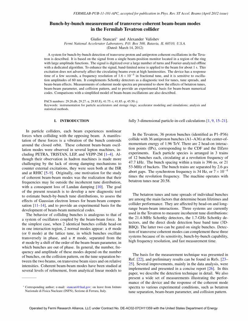
The basic features of transverse coherent oscillations canbe described by a simple model. In the Tevatron, these oscil-lations are substantially nonlinear due to the properties of thelattice and of the beam-beam force. Hence, the rigid bunchapproximation cannot provide an accurate view of the co-herent mode spectrum. However, this approximation can beused for qualitative analysis of the expected beam-beam modetunes and their dependence on the the betatron tunes Q and thebeam-beam parameter per interaction point ξ .

We use a simple matrix formalism to compute the eigen-mode tunes of the system of colliding bunches. Besides em-ploying the rigid bunch approximation, one more simplifica-tion is used. The complete description of the system would re-quire modeling the interaction of 72 bunches at 138 collisionpoints. The analysis of such a system can be quite complex.Observations and analytical estimates show that the differencein tunes between individual bunches is small compared to thebeam-beam tune shift. Thus, as a first approximation, it is pos-sible to neglect long range interactions. This limits the systemto 6 bunches (3 in each beam) colliding at two head-on inter-action points. In the following discussion, we limit betatronoscillations to one degree of freedom. Because the system has

3-fold symmetry, the 1-turn map transporting the 12-vector ofdipole moments and momenta of the system of 6 bunches canbe expressed as follows:

M = MBB3 MT3 MBB2 MT2 MBB1 MT1, (1)

where MTN (N = 1,2,3) are the 2×2 block-diagonal 12×12matrices transporting phase space coordinates through the ac-celerator arcs, and MBBN are the matrices describing thinbeam-beam kicks at the IPs. Although there are only 2 in-teractions per bunch, 3 collision matrices are used to describea one-turn map of the system of six bunches. This construc-tion represents the time propagation of the bunch coordinatesthrough one turn with break points at the CDF (B0), D0 andF0 locations in the machine. If on a given step the bunch is atB0 or D0, its momentum coordinate is kicked according to thedistance between the centroids of this bunch and of the oppos-ing bunch. If the bunch is at F0 (1/3 of the circumference fromB0 and D0), where the beams are separated, its momentum isunchanged. For example, the matrix describing the interactionof proton bunch 1 with antiproton bunch 2 at CDF and protonbunch 3 with antiproton bunch 3 at DZero has the followingform:

MBB1 =

1 0 0 0 0 0 0 0 0 0 0 0−2πξ p/β 1 0 0 0 0 0 0 2πξ p/β 0 0 0

0 0 1 0 0 0 0 0 0 0 0 00 0 0 1 0 0 0 0 0 0 0 00 0 0 0 1 0 0 0 0 0 0 00 0 0 0 −2πξ p/β 1 0 0 0 0 2πξ p/β 00 0 0 0 0 0 1 0 0 0 0 00 0 0 0 0 0 0 1 0 0 0 00 0 0 0 0 0 0 0 1 0 0 0

2πξ a/β 0 0 0 0 0 0 0 −2πξ a/β 1 0 00 0 0 0 0 0 0 0 0 0 1 00 0 0 0 2πξ a/β 0 0 0 0 0 −2πξ a/β 1

. (2)

Here, ξ p and ξ a are the beam-beam parameters for protonsand antiprotons, and β is the amplitude function at the IP. TheYokoya factor [16, 27] is considered to be equal to 1. Theeigentunes of the 1-turn map are then computed numerically.

This model provides a quick estimate of the expected val-ues of the coherent beam-beam mode tunes for a given set ofmachine and beam parameters. The model cannot be usedfor accurate calculation of the relative amplitude of thesemodes, which is determined by nonlinear effects such as Lan-dau damping. For the case of weak nonlinearities, this ap-proach allows one to determine the mode amplitudes by com-puting the projection of mode eigenvectors on the excitationvector [4]. In the case of the Tevatron experiments describedbelow, this is not straightforward because a wideband noisesource was used to excite the beam motion.

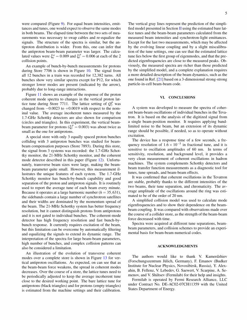
In Figure 1, an example of the dependence of the 6 eigenfre-

quencies on the beam-beam parameter per IP is presented. Asone would expect, at small values of ξ (uncoupled oscillators)the mode frequencies approach the bare lattice tunes; in thiscase, 0.587 for protons and 0.574 for antiprotons. When thetotal beam-beam parameter exceeds the difference betweenthe lattice tunes, the modes are split and their symmetry ap-proaches that of the conventional σ and π modes. The pa-rameters of this calculation are taken to resemble those of thebeginning of the Tevatron Store 7754, when the beam-beamparameter was ξ = ξ a = ξ p = 0.01. A comparison with datais given in Section V (Figure 13).

3

III. APPARATUS

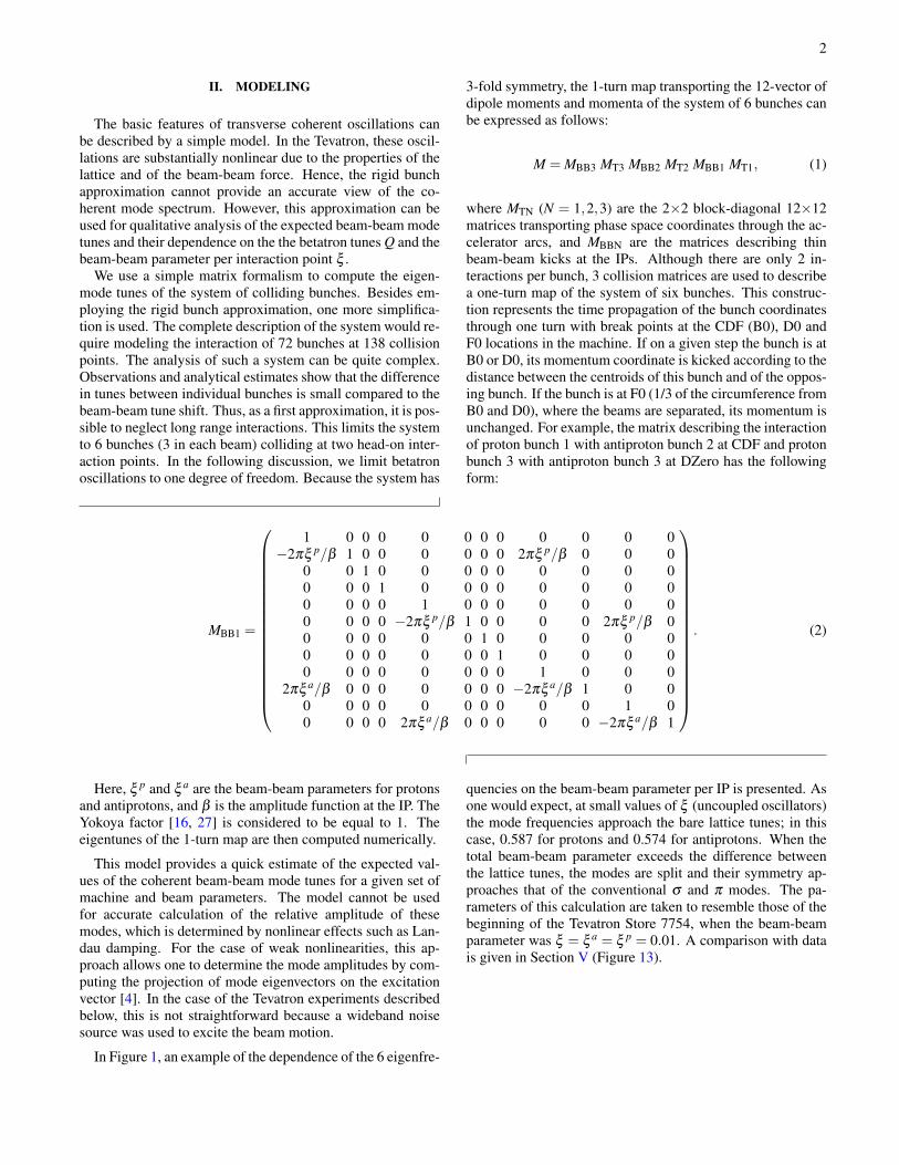
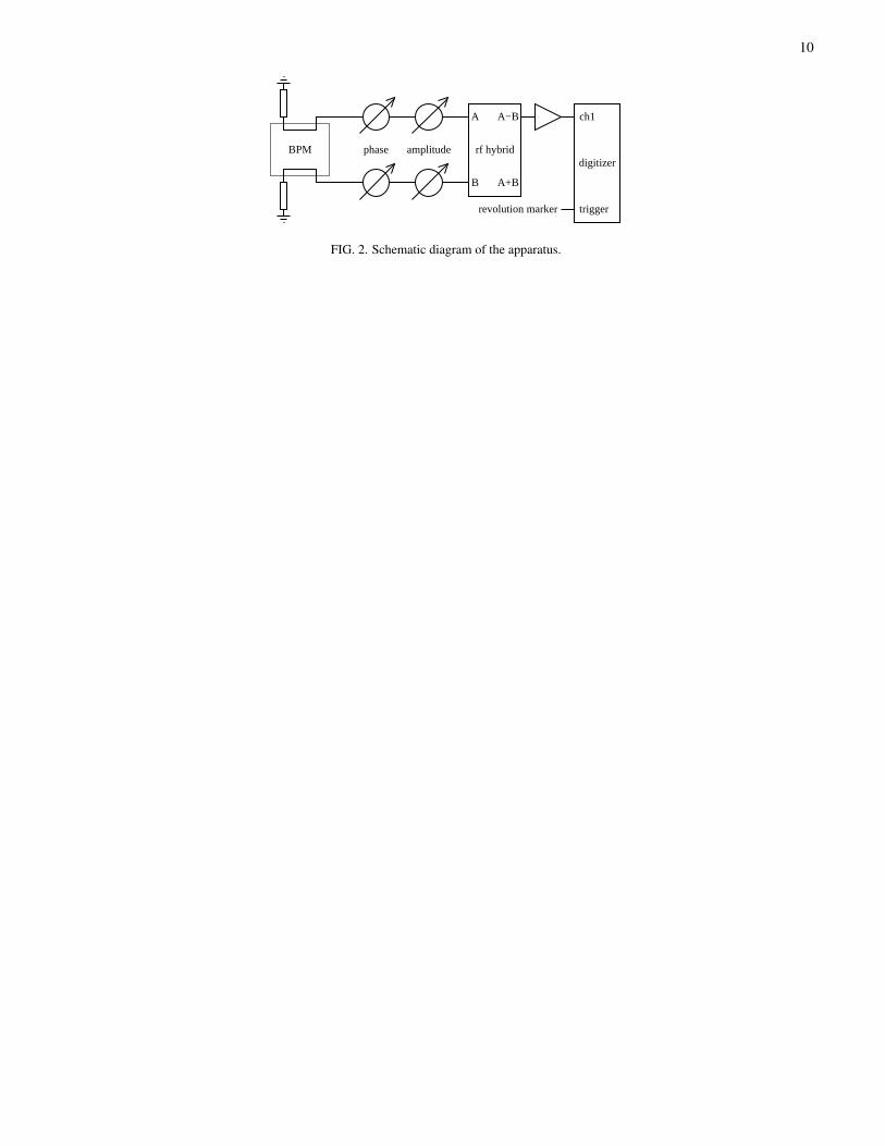
The system for the detection of transverse coherent modes(Figure 2) is based on the signal from a single vertical beam-position monitor (BPM) located near the CDF interactionpoint, in a region where the vertical amplitude function at col-lisions is βy = 880 m. The BPM is a stripline pickup, withtwo plate outputs (A and B) for each of the two counterpropa-gating beams. The proton outputs are split: half of the signalis sent to the Tevatron BPM readout and orbit stabilizationcircuits; the other half is used by the present system. Antipro-ton signals are about a factor three weaker and are usually notused for orbit feedback, so the splitter is not necessary and thefull signal can be analyzed. Switching between proton andantiproton signals presently requires physically swapping ca-bles.

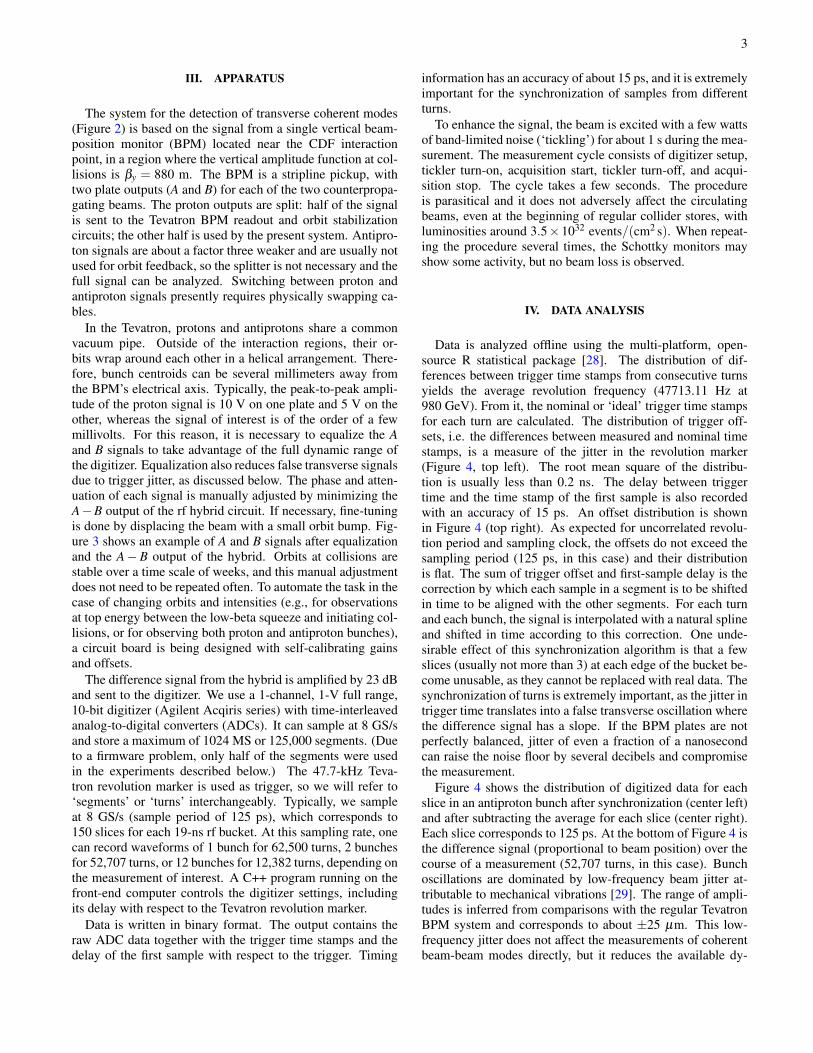
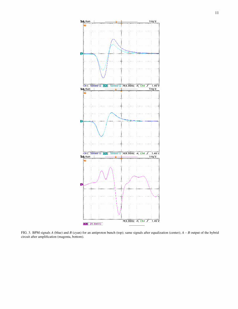
In the Tevatron, protons and antiprotons share a commonvacuum pipe. Outside of the interaction regions, their or-bits wrap around each other in a helical arrangement. There-fore, bunch centroids can be several millimeters away fromthe BPM’s electrical axis. Typically, the peak-to-peak ampli-tude of the proton signal is 10 V on one plate and 5 V on theother, whereas the signal of interest is of the order of a fewmillivolts. For this reason, it is necessary to equalize the Aand B signals to take advantage of the full dynamic range ofthe digitizer. Equalization also reduces false transverse signalsdue to trigger jitter, as discussed below. The phase and atten-uation of each signal is manually adjusted by minimizing theA−B output of the rf hybrid circuit. If necessary, fine-tuningis done by displacing the beam with a small orbit bump. Fig-ure 3 shows an example of A and B signals after equalizationand the A−B output of the hybrid. Orbits at collisions arestable over a time scale of weeks, and this manual adjustmentdoes not need to be repeated often. To automate the task in thecase of changing orbits and intensities (e.g., for observationsat top energy between the low-beta squeeze and initiating col-lisions, or for observing both proton and antiproton bunches),a circuit board is being designed with self-calibrating gainsand offsets.

The difference signal from the hybrid is amplified by 23 dBand sent to the digitizer. We use a 1-channel, 1-V full range,10-bit digitizer (Agilent Acqiris series) with time-interleavedanalog-to-digital converters (ADCs). It can sample at 8 GS/sand store a maximum of 1024 MS or 125,000 segments. (Dueto a firmware problem, only half of the segments were usedin the experiments described below.) The 47.7-kHz Teva-tron revolution marker is used as trigger, so we will refer to‘segments’ or ‘turns’ interchangeably. Typically, we sampleat 8 GS/s (sample period of 125 ps), which corresponds to150 slices for each 19-ns rf bucket. At this sampling rate, onecan record waveforms of 1 bunch for 62,500 turns, 2 bunchesfor 52,707 turns, or 12 bunches for 12,382 turns, depending onthe measurement of interest. A C++ program running on thefront-end computer controls the digitizer settings, includingits delay with respect to the Tevatron revolution marker.

Data is written in binary format. The output contains theraw ADC data together with the trigger time stamps and thedelay of the first sample with respect to the trigger. Timing

information has an accuracy of about 15 ps, and it is extremelyimportant for the synchronization of samples from differentturns.

To enhance the signal, the beam is excited with a few wattsof band-limited noise (‘tickling’) for about 1 s during the mea-surement. The measurement cycle consists of digitizer setup,tickler turn-on, acquisition start, tickler turn-off, and acqui-sition stop. The cycle takes a few seconds. The procedureis parasitical and it does not adversely affect the circulatingbeams, even at the beginning of regular collider stores, withluminosities around 3.5×1032 events/(cm2 s). When repeat-ing the procedure several times, the Schottky monitors mayshow some activity, but no beam loss is observed.

IV. DATA ANALYSIS

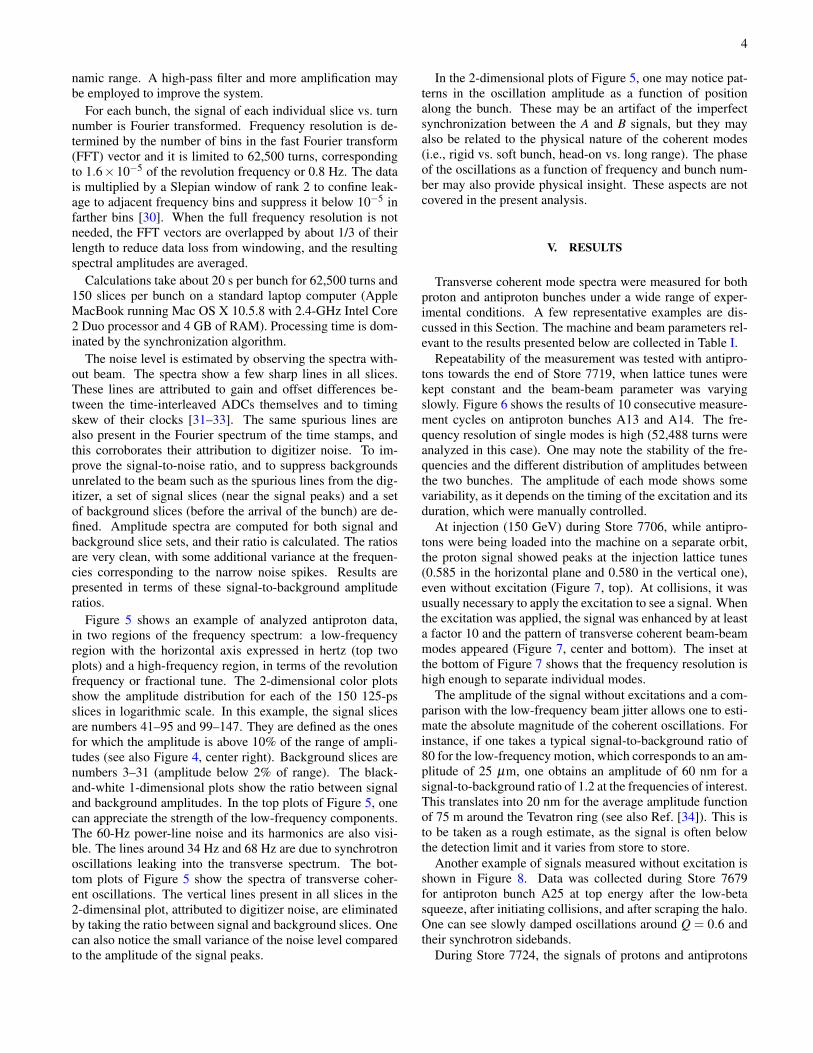
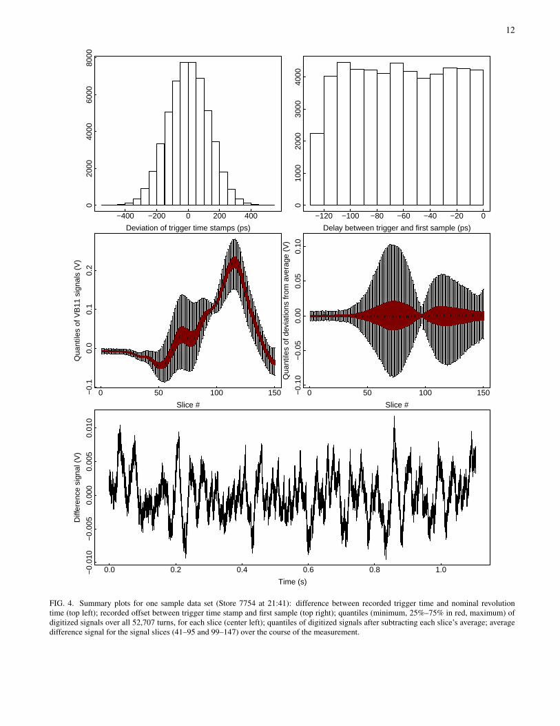
Data is analyzed offline using the multi-platform, open-source R statistical package [28]. The distribution of dif-ferences between trigger time stamps from consecutive turnsyields the average revolution frequency (47713.11 Hz at980 GeV). From it, the nominal or ‘ideal’ trigger time stampsfor each turn are calculated. The distribution of trigger off-sets, i.e. the differences between measured and nominal timestamps, is a measure of the jitter in the revolution marker(Figure 4, top left). The root mean square of the distribu-tion is usually less than 0.2 ns. The delay between triggertime and the time stamp of the first sample is also recordedwith an accuracy of 15 ps. An offset distribution is shownin Figure 4 (top right). As expected for uncorrelated revolu-tion period and sampling clock, the offsets do not exceed thesampling period (125 ps, in this case) and their distributionis flat. The sum of trigger offset and first-sample delay is thecorrection by which each sample in a segment is to be shiftedin time to be aligned with the other segments. For each turnand each bunch, the signal is interpolated with a natural splineand shifted in time according to this correction. One unde-sirable effect of this synchronization algorithm is that a fewslices (usually not more than 3) at each edge of the bucket be-come unusable, as they cannot be replaced with real data. Thesynchronization of turns is extremely important, as the jitter intrigger time translates into a false transverse oscillation wherethe difference signal has a slope. If the BPM plates are notperfectly balanced, jitter of even a fraction of a nanosecondcan raise the noise floor by several decibels and compromisethe measurement.

Figure 4 shows the distribution of digitized data for eachslice in an antiproton bunch after synchronization (center left)and after subtracting the average for each slice (center right).Each slice corresponds to 125 ps. At the bottom of Figure 4 isthe difference signal (proportional to beam position) over thecourse of a measurement (52,707 turns, in this case). Bunchoscillations are dominated by low-frequency beam jitter at-tributable to mechanical vibrations [29]. The range of ampli-tudes is inferred from comparisons with the regular TevatronBPM system and corresponds to about ±25 µm. This low-frequency jitter does not affect the measurements of coherentbeam-beam modes directly, but it reduces the available dy-

4

namic range. A high-pass filter and more amplification maybe employed to improve the system.

For each bunch, the signal of each individual slice vs. turnnumber is Fourier transformed. Frequency resolution is de-termined by the number of bins in the fast Fourier transform(FFT) vector and it is limited to 62,500 turns, correspondingto 1.6×10−5 of the revolution frequency or 0.8 Hz. The datais multiplied by a Slepian window of rank 2 to confine leak-age to adjacent frequency bins and suppress it below 10−5 infarther bins [30]. When the full frequency resolution is notneeded, the FFT vectors are overlapped by about 1/3 of theirlength to reduce data loss from windowing, and the resultingspectral amplitudes are averaged.

Calculations take about 20 s per bunch for 62,500 turns and150 slices per bunch on a standard laptop computer (AppleMacBook running Mac OS X 10.5.8 with 2.4-GHz Intel Core2 Duo processor and 4 GB of RAM). Processing time is dom-inated by the synchronization algorithm.

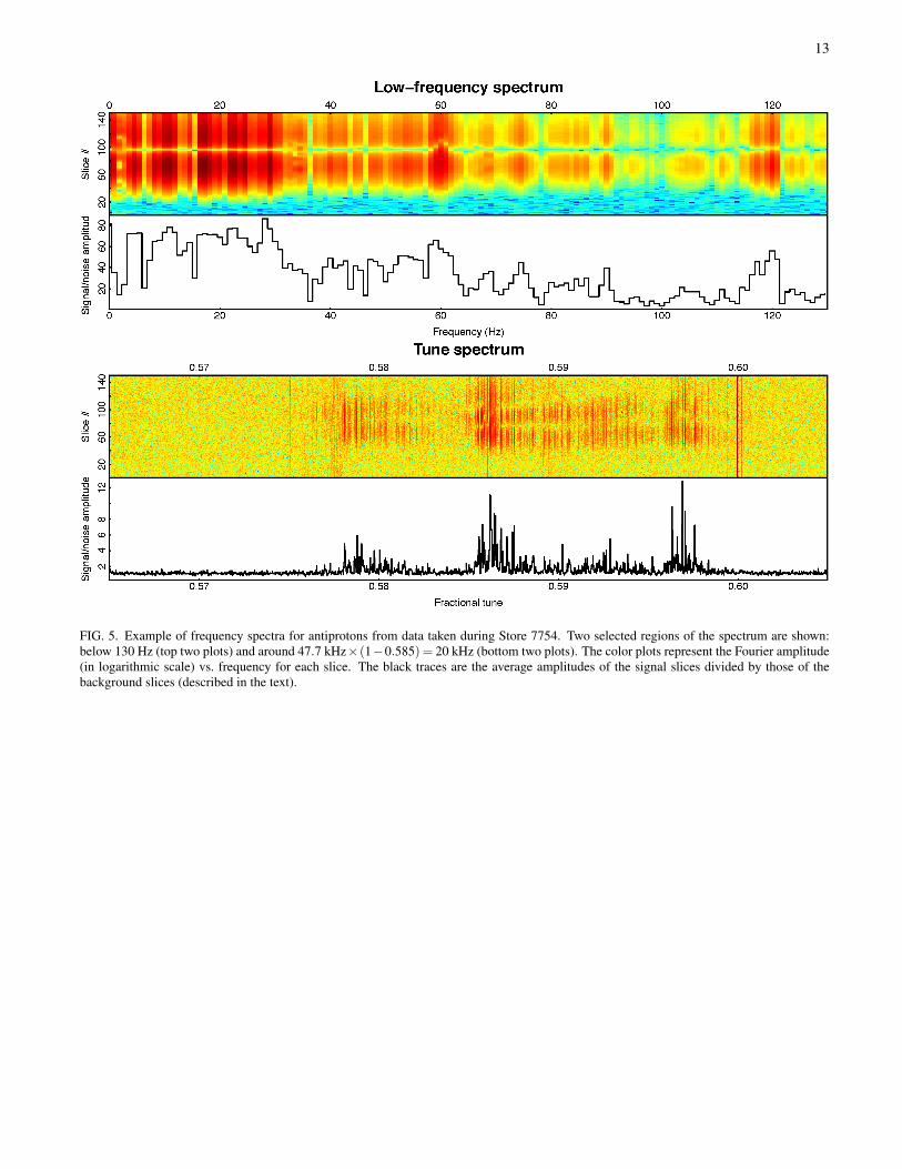
The noise level is estimated by observing the spectra with-out beam. The spectra show a few sharp lines in all slices.These lines are attributed to gain and offset differences be-tween the time-interleaved ADCs themselves and to timingskew of their clocks [31–33]. The same spurious lines arealso present in the Fourier spectrum of the time stamps, andthis corroborates their attribution to digitizer noise. To im-prove the signal-to-noise ratio, and to suppress backgroundsunrelated to the beam such as the spurious lines from the dig-itizer, a set of signal slices (near the signal peaks) and a setof background slices (before the arrival of the bunch) are de-fined. Amplitude spectra are computed for both signal andbackground slice sets, and their ratio is calculated. The ratiosare very clean, with some additional variance at the frequen-cies corresponding to the narrow noise spikes. Results arepresented in terms of these signal-to-background amplituderatios.

Figure 5 shows an example of analyzed antiproton data,in two regions of the frequency spectrum: a low-frequencyregion with the horizontal axis expressed in hertz (top twoplots) and a high-frequency region, in terms of the revolutionfrequency or fractional tune. The 2-dimensional color plotsshow the amplitude distribution for each of the 150 125-psslices in logarithmic scale. In this example, the signal slicesare numbers 41–95 and 99–147. They are defined as the onesfor which the amplitude is above 10% of the range of ampli-tudes (see also Figure 4, center right). Background slices arenumbers 3–31 (amplitude below 2% of range). The black-and-white 1-dimensional plots show the ratio between signaland background amplitudes. In the top plots of Figure 5, onecan appreciate the strength of the low-frequency components.The 60-Hz power-line noise and its harmonics are also visi-ble. The lines around 34 Hz and 68 Hz are due to synchrotronoscillations leaking into the transverse spectrum. The bot-tom plots of Figure 5 show the spectra of transverse coher-ent oscillations. The vertical lines present in all slices in the2-dimensinal plot, attributed to digitizer noise, are eliminatedby taking the ratio between signal and background slices. Onecan also notice the small variance of the noise level comparedto the amplitude of the signal peaks.

In the 2-dimensional plots of Figure 5, one may notice pat-terns in the oscillation amplitude as a function of positionalong the bunch. These may be an artifact of the imperfectsynchronization between the A and B signals, but they mayalso be related to the physical nature of the coherent modes(i.e., rigid vs. soft bunch, head-on vs. long range). The phaseof the oscillations as a function of frequency and bunch num-ber may also provide physical insight. These aspects are notcovered in the present analysis.

V. RESULTS

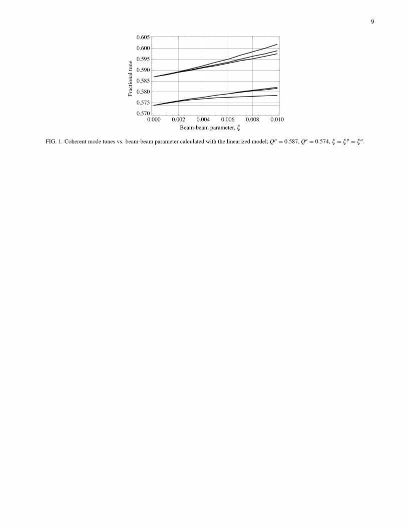
Transverse coherent mode spectra were measured for bothproton and antiproton bunches under a wide range of exper-imental conditions. A few representative examples are dis-cussed in this Section. The machine and beam parameters rel-evant to the results presented below are collected in Table I.

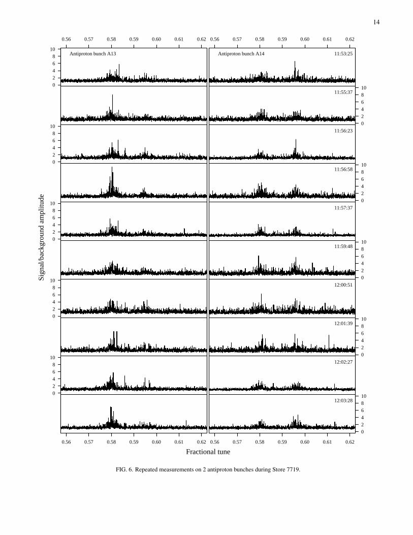
Repeatability of the measurement was tested with antipro-tons towards the end of Store 7719, when lattice tunes werekept constant and the beam-beam parameter was varyingslowly. Figure 6 shows the results of 10 consecutive measure-ment cycles on antiproton bunches A13 and A14. The fre-quency resolution of single modes is high (52,488 turns wereanalyzed in this case). One may note the stability of the fre-quencies and the different distribution of amplitudes betweenthe two bunches. The amplitude of each mode shows somevariability, as it depends on the timing of the excitation and itsduration, which were manually controlled.

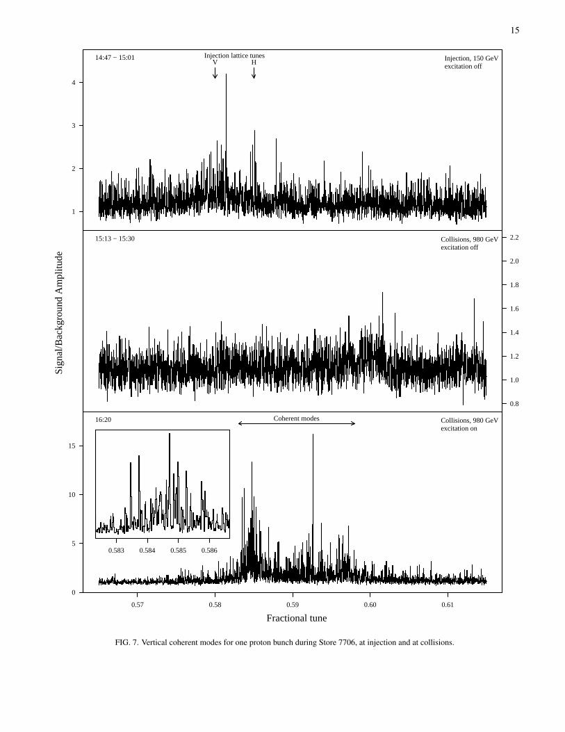
At injection (150 GeV) during Store 7706, while antipro-tons were being loaded into the machine on a separate orbit,the proton signal showed peaks at the injection lattice tunes(0.585 in the horizontal plane and 0.580 in the vertical one),even without excitation (Figure 7, top). At collisions, it wasusually necessary to apply the excitation to see a signal. Whenthe excitation was applied, the signal was enhanced by at leasta factor 10 and the pattern of transverse coherent beam-beammodes appeared (Figure 7, center and bottom). The inset atthe bottom of Figure 7 shows that the frequency resolution ishigh enough to separate individual modes.

The amplitude of the signal without excitations and a com-parison with the low-frequency beam jitter allows one to esti-mate the absolute magnitude of the coherent oscillations. Forinstance, if one takes a typical signal-to-background ratio of80 for the low-frequency motion, which corresponds to an am-plitude of 25 µm, one obtains an amplitude of 60 nm for asignal-to-background ratio of 1.2 at the frequencies of interest.This translates into 20 nm for the average amplitude functionof 75 m around the Tevatron ring (see also Ref. [34]). This isto be taken as a rough estimate, as the signal is often belowthe detection limit and it varies from store to store.

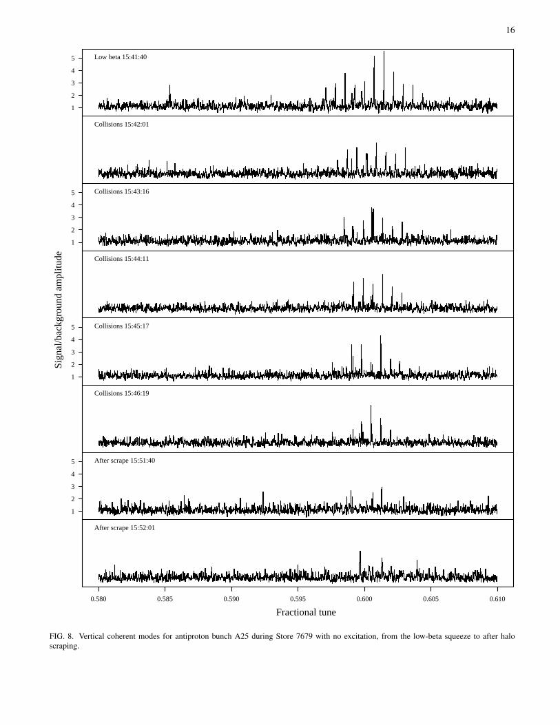
Another example of signals measured without excitation isshown in Figure 8. Data was collected during Store 7679for antiproton bunch A25 at top energy after the low-betasqueeze, after initiating collisions, and after scraping the halo.One can see slowly damped oscillations around Q = 0.6 andtheir synchrotron sidebands.

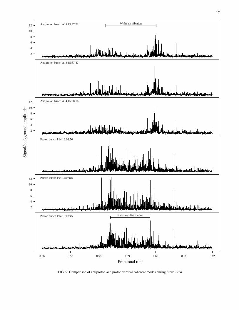
During Store 7724, the signals of protons and antiprotons

5

were compared (Figure 9). For equal beam intensities, emit-tances and tunes, one would expect to observe the same modesin both beams. The elapsed time between the two sets of mea-surements was necessary to swap cables and re-equalize thesignals. The structure of the spectra is similar, but the an-tiproton distribution is wider. From this, one can infer thatthe antiproton beam-beam parameter was larger. The calcu-lated values were ξ a

y = 0.009 and ξpy = 0.006 at each of the 2

collision points.An example of bunch-by-bunch measurements for protons

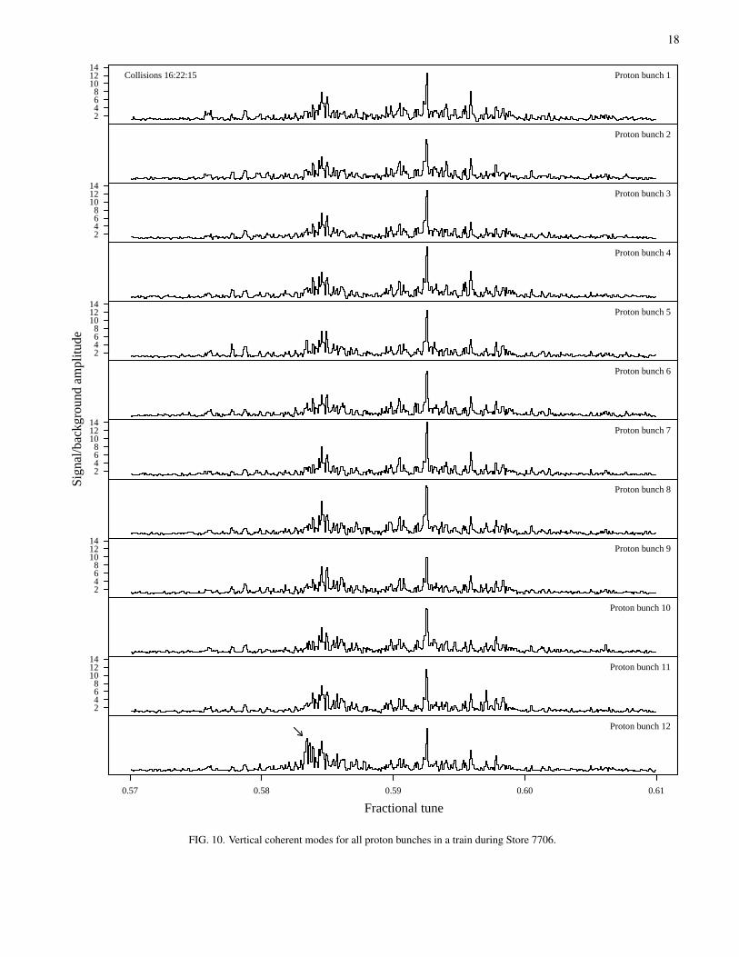
during Store 7706 is shown in Figure 10. The signal fromall 12 bunches in a train was recorded for 12,382 turns. Allbunches show very similar spectra except for P12, for whichstronger lower modes are present (indicated by the arrow),probably due to long-range interactions.

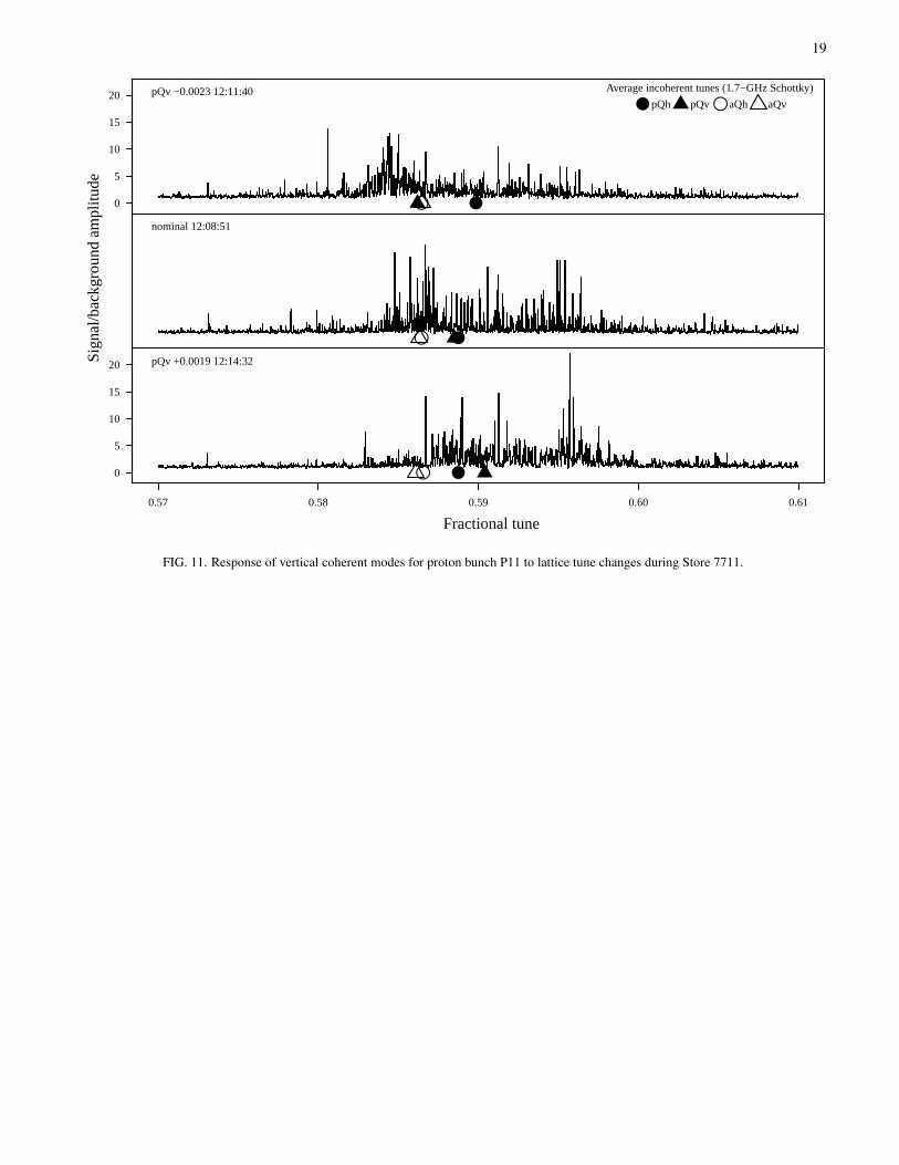
Figure 11 shows an example of the response of the protoncoherent mode spectra to changes in the vertical proton lat-tice tune during Store 7711. The lattice setting of Qp

y waschanged from −0.0023 to +0.0019 with respect to the nom-inal value. The average incoherent tunes measured by the1.7-GHz Schottky detectors are also shown for comparison(circles and triangles). In this experiment, the vertical beam-beam parameter for protons (ξ p

y = 0.003) was about twice assmall as the one for antiprotons.

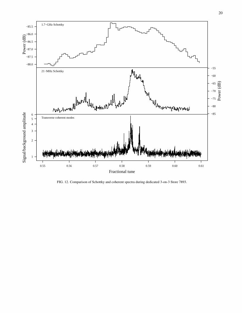
A special store with only 3 equally spaced proton bunchescolliding with 3 antiproton bunches was studied for beam-beam compensation purposes (Store 7893). During this store,the signal from 3 systems was recorded: the 1.7-GHz Schot-tky monitor, the 21-MHz Schottky monitor, and the coherentmode detector described in this paper (Figure 12). Unfortu-nately, transverse beam sizes were large, making the beam-beam parameter quite small. However, this measurement il-lustrates the unique features of each system. The 1.7-GHzSchottky monitor has bunch-by-bunch capability and goodseparation of the proton and antiproton signals. It is routinelyused to report the average tune of each beam every minute.Because it operates at a large harmonic number (h = 35,631),the sidebands contain a large number of synchrotron satellitesand their widths are dominated by the momentum spread ofthe beam. The 21-MHz Schottky system has better frequencyresolution, but it cannot distinguish protons from antiprotonsand it is not gated to individual bunches. The coherent-modedetector has high frequency resolution and fast bunch-by-bunch response. It currently requires excitation of the beam,but this limitation can be overcome by automatically filteringand equalizing the signals to extend its dynamic range. Theinterpretation of the spectra for large beam-beam parameters,high number of bunches, and complex collision patterns canalso be considered a limitation.

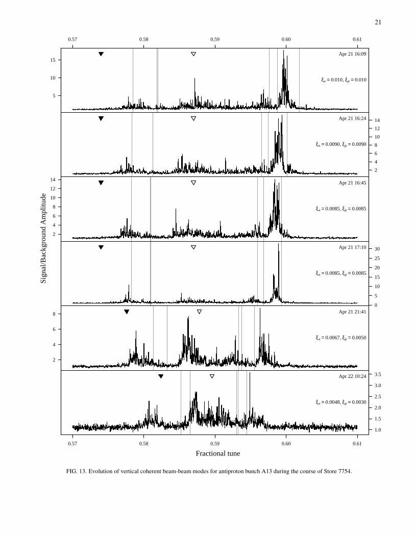
An illustration of the evolution of transverse coherentmodes over a complete store is shown in Figure 13 for ver-tical antiproton oscillations. As expected, on can see that asthe beam-beam force weakens, the spread in coherent modesdecreases. Over the course of a store, the lattice tunes need tobe periodically adjusted to keep the average incoherent tuneclose to the desired working point. The bare lattice tune forantiprotons (black triangles) and for protons (empty triangles)is estimated from the machine settings and their calibration.

The vertical gray lines represent the prediction of the simpli-fied model presented in Section II using the estimated bare lat-tice tunes and the beam-beam parameters calculated from themeasured beam intensities and synchrotron-light emittances.Except for the last two measurements, which may be affectedby the evolving linear coupling and by a slight miscalibra-tion of the tune settings, one can see that the estimated latticetune lies below the first group of eigenmodes, and that the pre-dicted eigenfrequencies are close to the measured peaks. Ob-viously, the measured spectra are richer than those predictedby the simplified model, and a complete explanation requiresa more detailed description of the beam dynamics, such as theone found in Ref. [21] based on a 3-dimensional strong-strongparticle-in-cell beam-beam code.

VI. CONCLUSIONS

A system was developed to measure the spectra of coher-ent beam-beam oscillations of individual bunches in the Teva-tron. It is based on the analysis of the digitized signal froma single beam-position monitor. It requires applying band-limited noise to the beam, but an extension of its dynamicrange should be possible, if needed, so as to operate withoutexcitation.

The device has a response time of a few seconds, a fre-quency resolution of 1.6× 10−5 in fractional tune, and it issensitive to oscillation amplitudes of 60 nm. In terms ofsensitivity, resolution, and background level, it provides avery clean measurement of coherent oscillations in hadronmachines. The system complements Schottky detectors andbeam transfer function measurements as a diagnostic tool fortunes, tune spreads, and beam-beam effects.

It was confirmed that coherent oscillations in the Tevatronare stable, probably thanks to the different intensities of thetwo beams, their tune separation, and chromaticity. The av-erage amplitude of the oscillations around the ring was esti-mated to be of the order of 20 nm.

A simplified collision model was used to calculate modeeigenfrequencies and to show their dependence on the beam-beam coupling. It was compared with observations made overthe course of a collider store, as the strength of the beam-beamforce decreased with time.

Spectra were acquired at different tune separations, beam-beam parameters, and collision schemes to provide an experi-mental basis for beam-beam numerical codes.

ACKNOWLEDGMENTS

The authors would like to thank V. Kamerdzhiev(Forschungszentrum Julich, Germany), F. Emanov (BudkerInstitute for Nuclear Physics, Novosibirsk, Russia), Y. Alex-ahin, B. Fellenz, V. Lebedev, G. Saewert, V. Scarpine, A. Se-menov, and V. Shiltsev (Fermilab) for their help and insights.

Fermilab is operated by Fermi Research Alliance, LLCunder Contract No. DE-AC02-07CH11359 with the UnitedStates Department of Energy.

6

[1] A. Piwinski, IEEE Trans. Nucl. Sci. 26, 4268 (1979).[2] T. Ieiri, T. Kawamoto, and K. Hirata, Nucl. Instrum. Methods

Phys. Res. A 265, 364 (1988).[3] E. Keil, K. Cornelis, and K. Hirata, in Proc. 15th Int. Conf. on

High Energy Accel., Hamburg, Germany, 1106 (1992), http://cdsweb.cern.ch/record/239617.

[4] I. N. Nesterenko, E. A. Perevedentsev, and A. A. Valishev, Phys.Rev. E 65, 056502 (2002).

[5] J. P. Koutchouk, CERN Report ISR-OP/JPK-svw (19 March1982), http://cdsweb.cern.ch/record/1131719.

[6] J. P. Koutchouk, CERN Report ISR-OP/JPK-bm (15 June1982), http://cdsweb.cern.ch/record/1131796.

[7] W. Fischer et al., BNL Report C-AD/AP/75 (2002).[8] W. Fischer et al., in Proc. 2003 Part. Accel. Conf. (PAC03),

135 (2003).[9] T. Pieloni, Ph.D. thesis, Ecole Polytechnique Federale de Lau-

sanne, Switzerland, 2008.[10] Y. Alexahin, Part. Accel. 59, 43 (1998).[11] V .Shiltsev et al., Phys. Rev. ST Accel. Beams 2,

071001 (1999).[12] V. Shiltsev et al., New J. Phys. 10, 043042 (2008).[13] V. Shiltsev et al., Phys. Rev. ST Accel. Beams 11,

103501 (2008).[14] A. Valishev and G. Stancari, in Proc. 2011 Part. Accel. Conf.

(PAC11), New York, New York, (2011), p. 67.[15] R. E. Meller and R. H. Siemann, IEEE Trans. Nucl. Sci. 28,

2431 (1981).[16] K. Yokoya and H. Koiso, Part. Accel. 27, 181 (1990).[17] W. Herr, M. P. Zorzano, and F. Jones, Phys. Rev. ST Accel.

Beams 4, 054402 (2001).[18] Y. Alexahin, Nucl. Instrum. Methods Phys. Res. A 480,

253 (2002).[19] T. Pieloni and W. Herr, in Proc. 2005 Part. Accel. Conf.

(PAC05), Knoxville, Tennessee, 4030 (2005).

[20] J. Qiang et al., Nucl. Instrum. Methods Phys. Res. A 558,351 (2006).

[21] E. G. Stern et al., Phys. Rev. ST Accel. Beams 13,024401 (2010).

[22] J.-P. Carneiro et al., Fermilab Report Beams-doc-1911-v1,http://beamdocs.fnal.gov (unpublished).

[23] A. Semenov et al., in Proc. 2007 Part. Accel. Conf. (PAC07),Albuquerque, New Mexico, 3877 (2007).

[24] V. Kamerdzhiev, V. Lebedev, and A. Semenov, in Proc. 2008Beam Instrum. Workshop (BIW08), Tahoe City, California,300 (2008).

[25] A. Valishev et al., in Proc. 2008 Eur. Part. Accel. Conf.(EPAC08), Genoa, Italy, 3158 (2008).

[26] G. Stancari, A. Valishev, and A. Semenov, in Proc. 2010Beam Instrum. Workshop (BIW10), Santa Fe, New Mexico,363 (2010).

[27] K. Yokoya, Phys. Rev. ST Accel. Beams 3, 124401 (2000).[28] R Development Core Team, R: A language and environment for

statistical computing (R Foundation for Statistical Computing,Vienna, Austria, 2010), ISBN 3-900051-07-0, http://www.R-project.org.

[29] B. Baklakov et al., in Proc. 1999 Part. Accel. Conf. (PAC99),New York, New York, 1387 (1999).

[30] W. H. Press et al., Numerical Recipes: The Art of ScientificComputing (Cambridge University Press, 3rd ed., 2007).

[31] N. Kurosawa et al., IEEE Proc. Instrum. Meas. Tech. Conf. 2,763 (2000).

[32] J. Elbornsson, F. Gustafsson, and J.-E. Eklund, IEEE Trans. Sig.Proc. 53, 1413 (2005).

[33] P. Fong, A. Teruya, and M. Lowry, in Proc. Instrum. and Meas.Tech. Conf. (IMTC 2005), Ottawa, Canada (2005), p. 417.

[34] V. Shiltsev, in Proc. 2011 Part. Accel. Conf. (PAC11), NewYork, New York, THP067 (2011).

7

TAB

LE

S

TAB

LE

I.Su

mm

ary

ofex

peri

men

talc

ondi

tions

:in

stan

tane

ous

lum

inos

ity,L

;ave

rage

num

ber

ofpr

oton

san

dan

tipro

tons

per

bunc

h,N

p and

Na ;a

vera

getr

ansv

erse

emitt

ance

sfr

omth

esy

nchr

otro

nlig

htm

onito

r(9

5%,n

orm

aliz

ed),

εp x,ε

p y,ε

a x,a

ndε

a y;a

vera

gelo

ngitu

dina

lem

ittan

ces,

εp zan

dε

a z(1

stan

dard

devi

atio

n);a

vera

gein

cohe

rent

tune

sfr

omth

e1.

7-G

Hz

Scho

ttky

dete

ctor

,Qp x,Q

p y,Q

a x,an

dQ

a y;ca

lcul

ated

linea

rbea

m-b

eam

para

met

ers

peri

nter

actio

npo

int,

ξp x,ξ

p y,ξ

a x,a

ndξ

a y.

Stor

eD

ate

Tim

eL

Np

Na

εp x

εp y

εa x

εa y

εp z

εa z

Qp x

Qp y

Qa x

Qa y

ξp x

ξp y

ξa x

ξa y

1032/(c

m2

s)10

1110

11µ

mµ

mµ

mµ

meV

seV

s

7679

15M

ar20

1016

:00

3.35

02.

891

0.86

1916

.923

.57.

98.

73.

293.

270.

6038

0.59

140.

6175

0.59

810.

0078

0.00

740.

0115

0.00

9877

0625

Mar

2010

15:1

33.

500

2.95

30.

9117

15.9

22.1

8.8

8.8

3.29

2.96

0.60

820.

6138

0.62

350.

6126

0.00

760.

0076

0.01

250.

0106

7706

25M

ar20

1016

:22

2.67

02.

756

0.81

4417

.223

.78.

79.

73.

844.

030.

5910

0.59

040.

5876

0.58

600.

0067

0.00

630.

0108

0.00

9277

1126

Mar

2010

12:0

91.

430

2.82

20.

5842

22.5

31.3

11.6

13.8

4.71

4.59

0.58

880.

5889

0.58

680.

5868

0.00

350.

0032

0.00

840.

0072

7719

1A

pr20

1011

:58

0.81

02.

272

0.53

1923

.835

.618

.318

.36.

335.

520.

5880

0.58

810.

5875

0.58

660.

0021

0.00

210.

0063

0.00

5177

242

Apr

2010

15:3

82.

950

2.79

10.

8475

17.0

24.7

9.2

9.3

3.57

3.21

0.59

010.

5904

0.59

080.

5969

0.00

670.

0067

0.01

090.

0091

7724

2A

pr20

1016

:07

2.69

02.

752

0.81

9717

.425

.49.

59.

83.

733.

390.

5887

0.58

920.

5857

0.59

070.

0063

0.00

620.

0105

0.00

8777

5421

Apr

2010

16:0

93.

510

2.85

60.

9428

15.0

23.3

7.7

9.4

3.31

3.52

0.59

780.

5908

0.61

630.

6096

0.00

850.

0077

0.01

240.

0100

7754

21A

pr20

1016

:24

3.20

02.

810

0.92

3615

.123

.17.

99.

44.

413.

640.

5901

0.58

990.

5973

0.60

340.

0082

0.00

750.

0122

0.00

9977

5421

Apr

2010

16:4

52.

970

2.76

90.

9008

15.4

23.8

8.6

9.8

4.43

3.72

0.59

240.

5897

0.58

640.

5900

0.00

740.

0070

0.01

170.

0095

7754

21A

pr20

1017

:10

2.73

02.

737

0.88

0615

.824

.49.

010

.04.

503.

850.

5890

0.58

890.

5867

0.58

720.

0070

0.00

660.

0113

0.00

9177

5421

Apr

2010

21:4

11.

570

2.55

40.

7333

18.6

29.1

12.3

13.7

5.54

4.82

0.58

830.

5885

0.58

670.

5863

0.00

430.

0040

0.00

890.

0071

7754

22A

pr20

1010

:24

0.67

02.

241

0.50

7223

.836

.819

.620

.76.

856.

040.

5882

0.58

870.

5871

0.58

770.

0019

0.00

180.

0061

0.00

4978

9315

Jun

2010

13:2

60.

055

2.70

30.

4600

25.9

36.0

19.6

20.1

3.86

2.78

0.58

490.

5852

0.56

390.

5628

0.00

170.

0017

0.00

700.

0060

8

FIGURES

9

Frac

tiona

ltun

e

0.000 0.002 0.004 0.006 0.008 0.010

0.570

0.575

0.580

0.585

0.590

0.595

0.600

0.605

Beam-beam parameter, ξ

FIG. 1. Coherent mode tunes vs. beam-beam parameter calculated with the linearized model; Qp = 0.587, Qa = 0.574, ξ = ξ p = ξ a.

10

digitizerBPM phase amplitude rf hybrid

A

B A+B

A−B ch1

triggerrevolution marker

FIG. 2. Schematic diagram of the apparatus.

11

FIG. 3. BPM signals A (blue) and B (cyan) for an antiproton bunch (top); same signals after equalization (center); A−B output of the hybridcircuit after amplification (magenta, bottom).

12

Deviation of trigger time stamps (ps)

−400 −200 0 200 400

020

0040

0060

0080

00

Delay between trigger and first sample (ps)

−120 −100 −80 −60 −40 −20 0

010

0020

0030

0040

00

0 50 100 150−0.

10.

00.

10.

2

Slice #

Qua

ntile

s of

VB

11 s

igna

ls (

V)

0 50 100 150−0.

10−

0.05

0.00

0.05

0.10

Slice #

Qua

ntile

s of

dev

iatio

ns fr

om a

vera

ge (

V)

0.0 0.2 0.4 0.6 0.8 1.0−0.

010

−0.

005

0.00

00.

005

0.01

0

Time (s)

Diff

eren

ce s

igna

l (V

)

Store7754/2010_04_21_21_40_47 − 21h40m (bunch 1)

FIG. 4. Summary plots for one sample data set (Store 7754 at 21:41): difference between recorded trigger time and nominal revolutiontime (top left); recorded offset between trigger time stamp and first sample (top right); quantiles (minimum, 25%–75% in red, maximum) ofdigitized signals over all 52,707 turns, for each slice (center left); quantiles of digitized signals after subtracting each slice’s average; averagedifference signal for the signal slices (41–95 and 99–147) over the course of the measurement.

13

FIG. 5. Example of frequency spectra for antiprotons from data taken during Store 7754. Two selected regions of the spectrum are shown:below 130 Hz (top two plots) and around 47.7 kHz×(1−0.585) = 20 kHz (bottom two plots). The color plots represent the Fourier amplitude(in logarithmic scale) vs. frequency for each slice. The black traces are the average amplitudes of the signal slices divided by those of thebackground slices (described in the text).

14

02468

10

0.56 0.57 0.58 0.59 0.60 0.61 0.62

Antiproton bunch A13

02468

10

02468

10

02468

10

02468

10

0.56 0.57 0.58 0.59 0.60 0.61 0.62

0.56 0.57 0.58 0.59 0.60 0.61 0.62

Antiproton bunch A14 11:53:25

0246810

11:55:37

11:56:23

0246810

11:56:58

11:57:37

0246810

11:59:48

12:00:51

0246810

12:01:39

12:02:27

0246810

12:03:28

0.56 0.57 0.58 0.59 0.60 0.61 0.62

Fractional tune

Sig

nal/b

ackg

roun

d am

plitu

de

FIG. 6. Repeated measurements on 2 antiproton bunches during Store 7719.

15

1

2

3

4

14:47 − 15:01 Injection, 150 GeVexcitation off

Injection lattice tunesHV

0.8

1.0

1.2

1.4

1.6

1.8

2.0

2.215:13 − 15:30 Collisions, 980 GeVexcitation off

0

5

10

15

16:20 Collisions, 980 GeVexcitation on

Coherent modes

0.57 0.58 0.59 0.60 0.61

0.583 0.584 0.585 0.586

Fractional tune

Sig

nal/B

ackg

roun

d A

mpl

itude

FIG. 7. Vertical coherent modes for one proton bunch during Store 7706, at injection and at collisions.

16

1

2

3

4

5 Low beta 15:41:40

Collisions 15:42:01

1

2

3

4

5 Collisions 15:43:16

Collisions 15:44:11

1

2

3

4

5 Collisions 15:45:17

Collisions 15:46:19

1

2

3

4

5 After scrape 15:51:40

0.580 0.585 0.590 0.595 0.600 0.605 0.610

After scrape 15:52:01

Fractional tune

Sig

nal/b

ackg

roun

d am

plitu

de

FIG. 8. Vertical coherent modes for antiproton bunch A25 during Store 7679 with no excitation, from the low-beta squeeze to after haloscraping.

17

2

4

6

8

10

12Wider distributionAntiproton bunch A14 15:37:21

Antiproton bunch A14 15:37:47

2

4

6

8

10

12 Antiproton bunch A14 15:38:16

Proton bunch P14 16:06:50

2

4

6

8

10

12 Proton bunch P14 16:07:15

Narrower distribution

0.56 0.57 0.58 0.59 0.60 0.61 0.62

Proton bunch P14 16:07:45

Fractional tune

Sig

nal/b

ackg

roun

d am

plitu

de

FIG. 9. Comparison of antiproton and proton vertical coherent modes during Store 7724.

18

2468

101214

Collisions 16:22:15 Proton bunch 1

Proton bunch 2

2468

101214

Proton bunch 3

Proton bunch 4

2468

101214

Proton bunch 5

Proton bunch 6

2468

101214

Proton bunch 7

Proton bunch 8

2468

101214

Proton bunch 9

Proton bunch 10

2468

101214

Proton bunch 11

0.57 0.58 0.59 0.60 0.61

Proton bunch 12

Fractional tune

Sig

nal/b

ackg

roun

d am

plitu

de

FIG. 10. Vertical coherent modes for all proton bunches in a train during Store 7706.

19

x

y

●●0

5

10

15

20 pQv −0.0023 12:11:40● ●

Average incoherent tunes (1.7−GHz Schottky)

pQh pQv aQh aQv

x

y

●●

nominal 12:08:51

x

y

●●

0.57 0.58 0.59 0.60 0.61

0

5

10

15

20 pQv +0.0019 12:14:32

Fractional tune

Sig

nal/b

ackg

roun

d am

plitu

de

FIG. 11. Response of vertical coherent modes for proton bunch P11 to lattice tune changes during Store 7711.

20

−88.0

−87.5

−87.0

−86.5

−86.0

−85.5P

ower

(dB

)1.7−GHz Schottky

−85

−80

−75

−70

−65

−60

−55

Pow

er (

dB)

21−MHz Schottky

1

2

3

4

5

6

0.55 0.56 0.57 0.58 0.59 0.60 0.61

Sig

nal/b

ackg

roun

d am

plitu

de

Transverse coherent modes

Fractional tune

FIG. 12. Comparison of Schottky and coherent spectra during dedicated 3-on-3 Store 7893.

21

x

y

5

10

15

0.57 0.58 0.59 0.60 0.61

Apr 21 16:09

ξa = 0.010, ξp = 0.010

x

y

2

4

6

8

10

12

14Apr 21 16:24

ξa = 0.0090, ξp = 0.0090

x

y

2

4

6

8

10

12

14Apr 21 16:45

ξa = 0.0085, ξp = 0.0085

x

y

0

5

10

15

20

25

30Apr 21 17:10

ξa = 0.0085, ξp = 0.0085

x

y

2

4

6

8 Apr 21 21:41

ξa = 0.0067, ξp = 0.0050

x

y

1.0

1.5

2.0

2.5

3.0

3.5

0.57 0.58 0.59 0.60 0.61

Apr 22 10:24

ξa = 0.0048, ξp = 0.0030

Fractional tune

Sig

nal/B

ackg

roun

d A

mpl

itude

FIG. 13. Evolution of vertical coherent beam-beam modes for antiproton bunch A13 during the course of Store 7754.