Bundling, Rationing, and Dispersion Strategies in Private and Common Value Auctions ∗ Ulf Axelson SIFR and SSE E-mail: [email protected]October 6, 2008 Abstract I study optimal selling strategies by a multi-product seller who is confined to using a standard auction format but has leeway in bundling products and choosing aggregate and individual quantities offered to buyers. I show how decisions of bundling, rationing, and dispersing the allocation depend on whether the product is of private or common value, how high demand is relative to supply, and what auction mechanism the seller uses. ∗ Preliminary and incomplete. 1
I study optimal selling strategies by a multi-product seller who is confined to using
a standard auction format but has leeway in bundling products and choosing aggregate
and individual quantities offered to buyers. I show how decisions of bundling, rationing,
and dispersing the allocation depend on whether the product is of private or common
value, how high demand is relative to supply, and what auction mechanism the seller
uses.
∗Preliminary and incomplete.
1
1. Introduction
This paper studies packaging and rationing choices faced by a multi-product, multi-unit seller
when buyers have private information about tastes. In this environment, a profit maximizing
seller has an incentive to design the selling mechanism in such a way as to extract as much
surplus as possible from buyers. There are (at least) three instruments at the sellers disposal
to accomplish this:
• Bundling: A multi-product seller has a choice between selling each product separatelyor tying the purchase of one product to the purchase of another. Examples of bundling
in product markets abound - a notorious example in later years being the strategy of
Microsoft to bundle software with their sale of operating systems. Another example,
studied by Stigler [18], is the practice of movie theaters to bundle ticket sales for
consecutive shows (“block booking”). In financial markets, the practice of pooling
assets and selling a single security with claims to all of them is commonplace for loans
and stocks.
• Rationing: The seller has two ways of restricting the aggregate quantity sold. One wayis to withhold some of the quantity from the market. Another way is to set a reserve
price below which no purchase can me made. In the monopoly pricing literature, this
is the classical way for a monopolist to increase profits at the expense of efficiency.
• Dispersion: On top of deciding whether differentiated products should be bundledor not, the seller also has to decide what quantity of each product a bundle should
contain. Should products be sold unit by unit, or in larger packages? I call this
a dispersion choice because within an auction context it involves deciding whether
to spread out the quantity sold over a larger set of winning bidders or whether to
keep the allocation concentrated. In consumer markets, the choice of package size is
an important marketing variable. In financial markets, the practice of dispersion is
widespread in, for example, the allocation of initial public offerings, where bidders
often get rewarded less than their demanded quantity even though they bid a higher
price than the market clearing price.
I argue that regardless of the bargaining or market power of the seller, he will typically
have a lot of leeway in using these three instruments (except possibly for setting a reserve
price). Of course, if the seller has complete latitude over the choice of selling mechanism,
these instruments will all be embedded in a larger mechanism design choice which also
2
involves constructing the optimal auction format. I argue, however, that it is often reasonable
to assume that the seller may be constrained to using a standard auction when selling his
products. There are several reasons for this. First, the format may be predetermined by the
market and is not easily adaptable to every single seller. Second, designing a complicated
novel mechanism can introduce a lot of confusion on the part of buyers. Third, the seller
may not be completely sure how to design the mechanism - it may depend in an intricate way
on assumptions about the distribution of buyers and may not be robust to small changes in
the market environment. For all of these reasons, I pay special attention to three standard
auction formats: Discriminatory price auctions, in which bidders submit sealed bids and
winning bidders pay their bids, uniform price auction, in which winning bidders all pay the
bid of the pivotal bidder, and ascending price auctions, in which bidders drop out as the
price rises until demand equals supply. I also discuss mechanisms that are more attractive
to the seller (when they exist), and study how bundling, rationing, and dispersion strategies
vary with the auction format.
A further goal of the paper is to characterize how these strategies vary with the product
characteristics. In particular, I distinguish between private value products such as consumer
goods where the valuation of a buyer is not affected by the valuation of others, and com-
mon value products such as financial assets where everyone has the same intrinsic value of
consumption but have differing information about the true value of the asset.
The set-up of the paper is as follows: A single risk-neutral seller has I independent
products to sell and a fixed quantity Q of each. There are N risk-neutral bidders, each of
whom gets a signal about each product. The valuation contains a private and a common
value component, and I assume that valuations across products are independent (thus, there
are no complementarities between products). I also assume that buyers have a constant
marginal value of consumption up to a quantity threshold normalized at one, after which
they have zero marginal value of consumption.
The results of the paper can be summarized as follows. First, I study the independent
private value case. With independent private values all the standard auction formats are
revenue equivalent, and are often optimal mechanisms. I first show that the seller wants
to concentrate the allocation as much as possible when values are private; that is, zero
dispersion is optimal. Thus, winning bidders get allocated a full unit. This is natural, since
the highest bidders are the ones with the highest marginal valuation of the products.
I also reaffirm the standard monopoly pricing result that some rationing is optimal. The
seller always wants to set a non-zero reserve price to increase overall payments, even at the
3
expense of not always selling the full quantity. I show that setting an optimal reserve price
is a better instrument for rationing than withholding quantity from the market ex ante.
Indeed, once the optimal reserve price is set, the seller does not withhold any quantity as
long as bids are above the reserve price. On the other hand, if the seller cannot set a reserve
price, withholding some quantity ex ante is typically optimal.
I go on to show that the choice of whether to bundle products or sell them separately
depends critically on the ratio of supply to “effective” demand, where effective demand is
the expected number of bidders with a positive valuation. When the supply is small relative
to demand, separate sales are typically optimal, while bundling is typically optimal when
the supply is large relative to demand (cf Palfrey [16] who developed similar results for the
case of one unit). The intuition is that when the supply is small relative to demand, the
pivotal price setting bidder will likely be closer to the top of the distribution, while when
supply is large he will likely be closer to the bottom. Therefore, since bundling will tend to
push valuations towards the center of the distribution, it is beneficial in the second case but
not in the first.
I also show how efficiency relates to the optimal choices of the seller. The choice of optimal
concentration is efficient, while rationing and bundling introduces inefficiencies. A reserve
price excludes some bidders with positive valuations, and bundling may cause a bidder with
a high valuation for one product to be excluded if he has a sufficiently low valuation for the
other product. Interestingly, bundling tends to reduce the first inefficiency by lowering the
optimal reserve price, and so there is no obvious efficiency ranking between bundled and
separate sales. I show that when the number of products is sufficiently large and the supply
is sufficiently large, bundled sales may be both optimal and efficient relative to separate
sales. In fact, in the limit as the number of products grows large and the supply is as big
as the effective demand, maximal bundling will both extract the total consumer surplus and
be socially efficient. On the other hand, if supply is sufficiently small, separate sales are
optimal and efficient. In the middle region, there are typically situations where the optimal
bundling strategy is inefficient.
I next study correlated private values. Most of the results for independent private values
goes through in this case. Maximal concentration is still optimal, as is setting a non-zero
reserve price. However, the reserve price is now a less efficient instrument for rationing, and
I show that it can be beneficial to restrict quantity ex ante even when the optimal reserve
price is set. The intuition for this is that with correlated values, bidders do not expect to face
the same distribution of competitors independent of their own signal. Thus, ideally a reserve
4
price should not be fixed, but should change with the conditional distribution of bidders -
when all values are relatively low, the reserve should be lower than otherwise. Decreasing the
aggregate quantity supplied approximates this type of conditional rationing. By reducing
the supply, the pivotal bidder’s valuation is increased, but only relative to the conditional
distribution of valuations.
The bundling decision will again depend in the same way on supply relative to demand,
but will now be affected by which auction format is being used. With correlated private
values, revenue equivalence still holds between uniform and ascending price auctions, but
as was established in Milgrom and Weber [14], discriminatory price auctions perform worse.
Since bundling tends to decrease valuation differences between bidders, it also decreases
the revenue differences between auction formats. Therefore, bundling will typically be a
substitute for choosing a better auction format, and I show that if the seller is forced to use
discriminatory price auctions, he will be more tempted to bundle. On the other extreme,
if the seller could utilize the optimal mechanism design, bundling would never occur. With
correlated values the seller can typically extract all surplus in a separate sale if he uses
the optimal mechanism, as has been shown by Myerson [15], Cremer and McLean [4], and
McAffee McMillan and Reny [10]. Thus, there is no room for either bundling, rationing, or
dispersion in this case (indeed, any of those strategies would reduce revenues).
For common value products, much of the analysis above changes dramatically. With
common values, all the standard auction formats can be revenue ranked, with ascending
price auctions being (weakly) superior to uniform price auction which in turn are (weakly)
superior to discriminatory price auctions. Selling strategies will differ between formats,
especially between the discriminatory price auction and the other two formats. I first show
that maximal concentration is typically optimal in discriminatory price auctions, but may or
may not be in uniform and ascending price auctions. In the private value case, concentration
was optimal because higher bidders had higher marginal values. With common values, a
higher bidder has a higher signal, but everyone has the same valuation function ex post (when
all information is revealed). It is therefore not too surprising that dispersion can be optimal.
In a uniform price auction, the price is set by the pivotal bidder, who takes into account the
information that he is pivotal when formulating his bid. When the allocation is concentrated,
the pivotal bidder tends to have a higher signal than most of his competitors, which increases
the winner’s curse and hence decreases his bid. By dispersing the concentration, the pivotal
bidder will tend to have a lower signal, but the winner’s curse will also diminish. Which of
these effects is stronger is not clear, and I show circumstances in which either can dominate.
5
In the discriminatory price auction, however, bidders use strategic bid-shading, which reduces
revenues to the seller. This strategic behavior is exacerbated when the allocation is dispersed,
as bidders do not have to worry as much about not winning. This explains why maximal
concentration is typically optimal in discriminatory price auctions.
Rationing strategies also differ in common value auctions. I show that zero rationing
(setting a zero reserve price and offering the whole quantity) is often optimal in uniform and
ascending price auction, especially as the auction grows large. As the auction grows large (in
that the number of bidders and the quantity both grow large), the underpricing in uniform
and ascending price auction goes to zero. There is therefore no need for restricting the
quantity sold. On the other hand, in discriminatory price auctions the underpricing does not
go to zero as the auction grows large because of the strategic bid-shading discussed above.
Therefore, a non-zero reserve price and restricted quantity ex ante is typically optimal.
The choice of bundling decision will also be determined by different driving forces than in
private value auctions. I first show that, regardless of the size of supply relative to demand,
bundling is optimal in all auction formats if the seller has enough products to bundle. The
intution is simple: Bidders’ information about the average quality in a large bundle tends to
converge to the mean, so that there is no private information about the mean in the limit.
Therefore, the underpricing per unit goes to zero as the number of products goes to infinity.
On the other hand, I show that if we think of holding the number of products fixed, and let the
auction grow large, separate sales become optimal in ascending and uniform price auctions
under some distributional assumptions. As the auction grows large, the underpricing goes to
zero regardless of the bundling strategy, but the convergence rate is faster for separate sales.
This is because bidders tend to have less complex information about an individual asset,
and the informational distance between the pivotal losing bidder and the winning bidders
therefore tends to disappear quicker. For discriminatory price auctions, a similar result holds
if the allocation is very concentrated, because only then does the underpricing go to zero as
the auction grows large. When the supply is bigger, bundling is typically more attractive in
discriminatory price auctions even as the auction grows large.
The last point again illustrates the fact that bundling tends to be a substitute for an
inferior auction mechanism. However, I show that this is not a general theorem. In fact,
there are situations when bundling is optimal in ascending price auctions when separate sales
are optimal in uniform price auctions, even though the ascending price auction is superior.
Finally, I study the situation when products have both private and common value com-
ponents. Using a valuation function that is additively separable in the private and common
6
value components, I show that each component can be analyzed separately as in the discus-
sion above, and that the optimal choice of strategy reduces to choosing the strategy that
maximizes the sum of the two components. The weight on each part will depend on the auc-
tion format being used and how large the auction is. In particular, since the underpricing per
unit sold goes to zero on the common value part as the auction grows large if the ascending
or the uniform price auction is used, the bundling and dispersion decisions will be completely
determined by considering the private value component. On the other hand, rationing will
decrease the revenue raised on the common value part even in large auctions, and so there
will be less of a tendency for rationing than if the products were pure private value. Since
the discriminatory price auction does not feature zero underpricing on the common value
part unless the allocation is extremely concentrated, common value considerations will be
more important in discriminatory price auctions.
Literature Review (*Incomplete*)
Many aspects of this problem have already been studied. It should be stated up front that
especially the results for independent private values have close parallels in existing literature.
A stylized categorization of the results can be done as follows:
Private values, single unit, single product: Myerson [15] studied the mechanism design
problem showing that first price, second price, and english auctions are all revenue equivalent
and optimal, under some conditions. For affiliated private values, Myerson [15] and later
Cremer and McLean [4] also showed that all surplus could in fact be extracted.
Private values, multiple unit, single product: This problem has been studied by Harris
and Raviv [6] and Maskin and Riley [9]. For unit demand, revenue equivalence still holds,
and ascending, uniform, and discriminatory price auctions are still optimal (with the correct
reserve price). With downward sloping demand curves, these auctions are not optimal.
Rather, a non-linear posted pricing schedule is optimal. Even in the competetive limit, the
monopolist will produce too little. Also, Maskin and Riley show that for the consumer with
top tastes, marginal utility is set equal to marginal cost, and for all other types, marginal
utility is higher than marginal cost. In the regular case, if the hazard rate is nonincreasing,
then marginal utility is decreasing in type, showing that relatively lower types consume too
little - there is concentration to the top. That is, the allocation is concentrated relative to
first best. Note that this is not necessarily the case, however it is the case for the highest
type and for the parametrization we consider in this paper. If types are independent but
utilities depend on all other types, then the same condition hold for a non-decreasing hazard
rate. Jackson and Kremer [7] also provide an example of revenue-increasing bundling in
7
private value auctions when marginal utilities are decreasing.
Private values, single unit, multiple products: Palfrey [16] shows, for the case of exoge-
nously given auctions and independent products, that bundling is optimal with two bidders,
but not with many bidders. Chakraborthy [3] sharpens some of these results to give ex-
act conditions for when there is a critical number of bidders N above which separate sales
are optimal and below which pooling is optimal. However, Armstrong shows that this is
no longer true when the optimal mechanism is used. With the optimal mechanism, which
allows for endogenous bundling as a function of bids, allowing some probability of bundling
is optimal even for two bidders. In this paper, I show that Armstrong’s result is specific to
his binary set-up, and that bundling is often optimal with two bidders and one good even
when the optimal reserve price is set.
2. Model Set-Up
A single risk-neutral seller has I differentiated products to sell. Each product i is of quality
Zi, where Zi is a random variable. I assume that qualities are distributed identically and
independently according to the distribution function G (z). The seller’s supply of each prod-
uct is Q. There are N risk neutral bidders. Each bidder n privately observes a signal Xi,n
about each product i. The value V that a bidder attaches to consuming a bundle containing
q1, ..., qI units of the I products is given by
V (q1, ..., qI ,X1,n, ...,XI,n, Z1, ..., ZI) =IX
i=1
min (qi, 1) (tXi,n + (1− t)Zi) (2.1)
Thus, marginal utility is constant up to a quantity normalized to one, after which it is zero.
Xi,n is the private value component and Zi the common value component of the valuation.
The parameter t ∈ [0, 1] measures the relative importance of these components, with t = 1
corresponding to the pure private value case and t = 0 corresponding to the pure common
value case. I assume that products are neither substitutes nor complements, so that the
utility of consuming product i is independent of the consumption of product j.
Signals are independent across products, and I assume that conditional on a quality
realization Zi = z, signals about product i are distributed identically and independently
across bidders according to the distribution function F (x |z ) with density f (x |z ) withsupport in [x, x]. Sellers do not know the realization of any random variables, but bidders
can make an inference about Zi from observing the signal Xi,n. To be precise, I assume that
8
the monotone likelihood ratio property holds:
MLRP f(x|z )f(x0|z ) ≥
f(x|z0 )f(x0|z0 ) if x > x0, z > z0
TheMLRP assumption captures the notion that a higher signal is correlated with a higher
value, and implies together with the valuation function in 2.1 that values are affiliated (see
Milgrom and Weber [14]).
I assume that the seller is faced with an exogenously specified auction format when selling
his products, but that he has leeway in choosing the quantity he puts on the market and
the way products are bundled, both in terms of number of distinct products and in terms
of the quantity of each product sold to winning bidders. More specifically, the seller has the
following choice variables:
-A partition Π = {Π1, ...,ΠJ} of the I assets, such that J separate auctions are held, onefor each bundle of products. I call this a bundling strategy.
-A choice of aggregate quantity Qj ≤ Q for each bundle to put on the market and a
choice of reserve price rj below which no bundle is sold. I call this a rationing strategy.
-A choice of individual quantity qj allocated to each winning bidder, or, equivalently, a
choice of Kj =Qj
qj∈ {1, ..., N} of how many bidders are allocated a bundle, subject to the
lowest of them paying at least rj. I call this a dispersion strategy.
Thus, the auction for bundle Πj will be a multi-unit auction of Kj identical items, each
valued by bidder n at
Vj³qj, {Xi,n}i∈Πj , {Zi,n}i∈Πj
´= min (qj, 1)
⎛⎝tXi∈Πj
Xi,n + (1− t)Xi∈Πj
Zi,n
⎞⎠I study the following standard auction formats (which, as is discussed in more detail
below, are in increasing order of attractiveness to the seller):
1. Discriminatory price auction (DP): Each bidder submits a sealed bid bn and bundles
are awarded to the K highest bidders subject to bn ≥ r. Winning bidders pay their
bid.
2. Uniform price auction (UP): Each bidder submits a sealed bid bn and bundles are
awarded to the K highest bidders subject to bn ≥ r. Winning bidders pay the bid of
the K + 1:st highest bidder or r, whichever is larger.
3. Ascending price auction (AP): The price starts at r and is increased continuously
throughout the auction, and bidders decide at each moment whether to stay in the
9
auction or drop out (irreversibly). Once all but K bidders have dropped out, the
auction stops and the remaining bidders are rewarded a bundle at the stopping price.
Given an auction format A ∈ {DP,UP,AP}, denote the revenues in auction j by πjA.
The seller’s maximization problem is then given as follows:
maxΠ,{Qj≤Q,rj ,Kj}J
j=1
JXj=1
E (πjA |Kj, Qj, rj ) (2.2)
I will also discuss how the results for the standard auction formats above differ from the
solutions where the seller has more power to choose an optimal mechanism. In particular,
one can think of two increasingly powerful levels of mechanism design accessible to the seller:
4. Optimal mechanism given a bundling strategy: Once the bundling strategy is picked,
revenue maximizing auctions are run under the restriction that a winner must be
awarded the same quantity of each product in bundle Πj.
5. Unrestricted optimal mechanism.
It is worth pointing out several restrictions imposed on the seller in Problem 2.2 relative
to mechanisms 4 and 5. Relative to mechanism 4, the standard auction formats impose a
restriction that all winning bidders are awarded the same quantities. This turns out not to
be an important restriction in most circumstances (see below), mainly due to the step-like
nature of the valuation function. More importantly, there is a severe restriction in how
payments and allocations are allowed to depend on the bids of competing bidders. This is
unimportant in the case of independent private values, but as has been shown by Myerson
[15], Cremer and McLean [4] and McAfee, McMillan and Reny [10] it is typically possible to
extract all bidder surplus in an optimal mechanism when bidders have correlated valuations.
In that case, allocations will be efficient if separate auctions for each product is run and
strategic components such as bundling, rationing, and dispersion have no bite.
Furthermore, relative to mechanism 5 the four other mechanisms have a restriction that
either the allocation of product i to bidder n is independent of Xi0n (if products i and i0 are
in different bundles), or as dependent on Xi0n as Xin (if they are in the same bundle). This
is not necessarily a feature of a revenue-maximizing mechanism. In fact, McAfee, McMillan,
and Whinston show in a monopoly pricing set-up that it is typically optimal to have the
allocation of i depend positively on Xi0n but less strongly so than on Xin, even in the case
of independent product values and independent private values. The solution to 2.2 will,
10
however, be qualitatively similar to the solution to the less restricted problem, and will often
come quite close to achieving the same level of revenues for the seller.
2.1. Equilibria of the auctions
To characterize equilibria for the three standard auction formats in the auction of bundle
Πj, denote by Xn and Z the sum of signals and qualities for the bundle, and by V (q,Xn, Z)
the valuation of the bundle:
Xn ≡Xi∈Πj
Xi,n
Z ≡Xi∈Πj
Zi
V (q,Xn, Z) ≡ min (q, 1) (tXn + (1− t)Z)
Equilibria for the three auction formats can then be found without any further restrictions
on the signal- and asset structure for the case of private values using the one-dimensional
aggregate signals Xn. In the case of common values (t < 1), however, equilibria can be quite
difficult to characterize, and a symmetric equilibrium may even fail to exist (see Jackson ).
The difficulty stems from the multi-dimensionality of the signals: It is in general not possible
to construct a sufficient statistic for the signals {Xi,n}i∈Πjthat also satisfies MLRP with
respect to Z. To circumvent these problems, I will frequently use the following distributional
assumption on signals and qualities when t < 1:
D1 Zi ∈ {0, 1}, Xi,n ∈ {0, 1}, P (Xi,n = 1 |Zi = 1) = p > P (Xi,n = 1 |Zi = 0) = q
Many of the results in the paper hold without invoking this assumption.
To allow for mixed strategies when signals are discretely distributed, denote by sn ∈ [0, 1]a random draw from a uniform distribution for each bidder that is independent of all other
variables. Also, denote by Y1 ≥ Y2 ≥ ... ≥ YN the N order statistics of the sample of
signals {Xi}Ni=1 , and by eY1 ≥ eY2 ≥ ... ≥ eYN the order statistics of the “augmented” signals{{Xi, si}}Ni=1 ordered lexicographically so that {Xi, si} > {Xj, sj} if Xi > Xj or if Xi = Xj
and si > sj. Similarly, define by Y −nK and eY −nK the K :th order statistic of the same samples
excluding {Xn} and {Xn, sn} respectively. The goal is now to find a bid-function bA (x, s)
for auction format A that describes bidding by an agent with signals Xn = x and sn = s
and constitutes a symmetric Bayesian Nash equilibrium. This can be done by a relatively
11
straight-forward extension of the analysis in Milgrom and Weber [14] to the multi-unit case
allowing for discretely distributed signals. Define a function v (x, y, s) by
v (x, y, s) = E³V (1,Xn, Z)
¯̄̄Xn = x, eY −nK = {y, s}
´Then the equilibrium bid functions are given in the following proposition.
Proposition 1. Suppose t = 1 or Πj is a singleton or assumption D1 holds, and the auction
has parameters {Q, r,K}. In all auction formats, bA (x, s) < r for {x, s} < {x∗, s∗} wherethe screening level {x∗, s∗} is defined as
{x∗, s∗} = infn{x, s}
¯̄̄E³V³q,Xn, Z
¯̄̄Xn = x, eY −nK < {x, s}
´≥ r
´oThe equilibrium bid function for the discriminatory price auction for {x, s} ≥ {x∗, s∗} isgiven by
The equilibrium bid function for the uniform price auction for {x, s} ≥ {x∗, s∗} is given by
bUP (x, s) = min (q, 1) ∗ v (x, x, s)
The equilibrium bid function for the ascending price auction is defined recursively as follows
for {x, s} ≥ {x∗, s∗}: SupposeM < N−K bidders do not participate at r. Define b0 (x, s |M )
as
b0 (x, s |M ) = E³V (q,Xn, Z)
¯̄̄Xn = x, eY −nK , ..., eY −nN−M−1 = {x, s} , eY −nN−M < {x∗, s∗}
´If the price reaches b0 (x, s |M ) without anyone else dropping out, drop out. If someone
drops out at p1 < b0AP (x, s |M ), define b1 (x, s |M,p1 ) as
b1 (x, s |M,p1 ) = E³V (q,Xn, Z)
¯̄̄Xn = x, eY −nK , ..., eY −nN−M−2 = {x, s} ,
b0³eY −nN−1−M
´= p1, eY −nN−M < {x∗, s∗} )
12
If the price reaches b1 (x, s |M,p1 ) without anyone else dropping out, drop out. Continue
similarly until the price reaches
bk (x, s |M,p1, ..., pk ) = E³V (q,Xn, Z)
¯̄̄Xn = x, eY −nK , ..., eY −nN−k−M−1 = {x, s} ,
bk−1³eY −nN−k−M
´= pk, ..., b
0³eY −nN−1−M
´= p1 )
where k more bidders have dropped out at prices pk ≥ pk−1 ≥ ... ≥ p1 and drop out when
the price reaches bk (x, s |M,p1, ..., pk ) if noone else has dropped out.
Proof. In Appendix.
Note that because the value function is additively separable in the private and common
value component, so is the bid function for all auction formats. Therefore, we can think of
the auction as two separate auction, one with a pure private value component and one with a
pure common value component, as long as we make sure that the screening level introduced
by the reserve price is the same as in the composite auction. This is the approach taken in
sections 3, 4, and 5 below. Section 6 then revisits the mixed case.
3. Independent Private Values
Suppose t = 1 and values are independently distributed. Proposition 1 shows that bids in the
uniform and ascending price auction are identical on the private value component, but differ
on the common values component, while the discriminatory price auction differs on both.
Thus, uniform and ascending price auctions raise exactly the same revenues when values are
private. In fact, as has been established for similar cases elsewhere, with independent private
values the discriminatory price auction raises the same expected revenues as well.
Lemma 1. Given {Πj, {Q, r} , q}, all three auction formats are revenue equivalent.
Proof. Omitted. Maskin and Riley [9] have proved revenue equivalence for the continuous
case. It is relatively straight-forward to extend the proof to the discrete case.1
It follows from Lemma 1 that the choice of bundling, rationing, and dispersion strategies
are not dependent on the particular auction format. I start by analyzing the dispersion
strategy and show that maximal concentration is always optimal in standard private value
auctions.
1However, it should be noted that revenue equivalence only holds in the discrete case if bids over thewhole interval
£X,X
¤are allowed. When values are discrete, it is typically optimal for the seller not to allow
bids over certain intervals (see Maskin and Riley () and Armstrong ()).
13
Proposition 2. q∗ = 1 for all auction formats.
Proof. Clearly, we can rule out q∗ > 1, since we can always reduce Q instead of allocating
extra quantity to bidders with zero marginal valuation. Given revenue equivalence, we can
confine study to the uniform price auction. From Proposition 1, the price per unit sold
will be max (YK+1, r) and the quantity sold will be qPK
i=1 1Yi≥r = QKi=1 1Yi≥r
K. Suppose
q < 1, and suppose you increase quantity to q0 = QK−1 . Then, the price per unit sold will
be max (YK , r) ≥ max (YK+1, r) and the quantity sold will be QK−1i=1 1Yi:N≥r
K−1 ≥ QKi=1 1Yi:N≥r
K.
Hence, expected revenue is increased.
Following Myerson [15], define the “virtual utility” J (x) as
J (x) ≡ x− 1− F (x)
f (x)
A regularity assumption that I will sometimes invoke is that J (x) is increasing:
Regularity F (x) is regular if the virtual utility J (x) is increasing in x.
This is a standard assumption in the mechanism design literature (see Myerson [15] and
Maskin and Riley [9]).
Define the set J0 as follows:
J0 =
(J−1 (0) J−1 (0) 6= ∅{0} J−1 (0) = ∅
That is, J0 contains the solutions to the equation J−1 (0) = 0 or {0} if no such solutionexists. The following proposition derives the optimal reserve price r∗ and shows that when
there is a chance of bidders’ valuation being below the valuation of the seller, a reserve price
strictly higher than the valuation of the seller is optimal.
Proposition 3. r∗ ∈ J0. If x≤ 0, there exists ε > 0 such that r∗ > ε for all Q,N .
Proof. Following Maskin and Riley, one can express the expected revenues (with q = 1)
as
E (π) = E
ÃQXn=1
1Yn≥rJ (Yn)
!(3.1)
Clearly, if J (x) is positive for all x, setting r to zero is optimal. If J (x) is negative somewhere,
r should be set at a point where J crosses 0 from below. Such a point exists, since J (x) =
x > 0. This proves the first part of the proposition. The second part follows from the
14
fact that J (x) is negative at x ≤ 0, so that the smallest solution to J (x) = 0 is strictly
positive.
The following proposition shows that under very mild assumptions, it is always optimal
to sell the full quantity Q if the seller can set the optimal reserve price. Thus, rationing
through the reserve price is always more efficient than rationing through the quantity put
on the market. However, if the seller does not have enough power to credibly set a reserve
price, decreasing the aggregate quantity can serve as a substitute.
Proposition 4. If J (x) = 0 has at most one solution, Q∗ = Q if the optimal reserve price
is set. If the seller is forced to set r = 0, there exists situations such that Q∗ < Q even when
x = 0 and Q < N .
Proof. If J (x) = 0 has at most one solution, it is positive above r∗. Hence, Expression
3.1 is strictly increasing in Q. Now suppose the seller is forced to set r = 0. Then, if QN→ 1
as N →∞, Expression 3.1 will be decreasing in Q at Q as N →∞, since J (0) < 0.I end the analysis of dispersion and rationing strategies by relating the standard auction
formats to the optimal mechanism given a bundling decision (format 4 above). As has been
established in Maskin and Riley [9], regularity actually implies that the standard auction
formats are optimal under the optimal rationing and dispersion strategies.
Proposition 5. (Maskin and Riley) If F (x) is regular, all auction formats with q∗ = 1, r∗ =
J0, Q∗ = Q are optimal mechanisms.
For non-regular distributions, Maskin and Riley show that the standard auction formats
perform worse than an ascending price auction with appropriately chosen discrete jumps in
the price increases, in which bidders who drop out just before a jump point get to share any
allocation that is left after distributing to remaining bidders. This will in effect create a type
of dispersion, since 0 < q < 1 for a range of bidder valuations. This should be contrasted
with the result in 2, which states that for the standard auction formats, dispersion is never
valuable.
I now turn to analyzing the bundling choice Π.. In light of Proposition 2, we can take
q given as one. The following two propositions show that the bundling decision will depend
on the ratio of demand to supply. The smaller the supply Q is relative to the number of
bidders, the more beneficial separate sales will be, and vice versa.
Proposition 6. Suppose the auction is regular and that x≥ 0. Then, there exists a β < 1
such that for all K, N there exists I such that if KN≥ β, bundling is optimal.
15
Proof. I start by establishing the folllowing Lemma:
Lemma 2. Suppose the auction is regular. Then, given K,N expected revenue per unit
π (K,N) is bounded by
E (YK+1) ≤ π (K,N) ≤(
1−F (r)K/N
r KN≥ 1− F (r)
(1− F )−1 (K/N) KN< 1− F (r)
Proof. E (YK+1) is the expected profit in a uniform price auction without reserve, and
hence serves as a lower bound for expected revenues. Now compare π (aK, aN) to π (K,N)
for a some integer larger than one. Then, π (aK, aN) ≥ π (K,N), since running a auctions
identical to the K,N auction yields aπ(K,N)a
= π (K,N) in expected revenues per unit. As a
goes to infinity, revenue in the optimal auction is given as in the right side of the Lemma.
It is now enough to show that π (K,N) is below the mean for KN≥ β for some β. Suppose
β = 1. Then,
π (K,N) ≤ (1− F (r)) r
=
Z x
r
rf (x) dx
<
Z x
x
xf (x) dx
Thus, there exists a β < 1 such that the statement holds.
Proposition 7. Suppose Q is given. Then there exists anM such that for all I, x, N ≥M ,
separate sales dominate bundling.
Proof. <<Extending Palfrey>>
Remark: These Propositions extend results in Palfrey [16] to the case of multiple units
and optimal reserve prices. He show that pooling is always optimal with two bidders when
there is no reserve. This result is modified when the optimal reserve price is taken into
account. Armstrong [1], for example, has shown that separate sales are always optimal for a
binary distribution when K = 1, even when N = 2. However, even with an optimal reserve
price, it is often the case that bundling dominates separate sales when N = 2. For example,
for one can sharpen the for symmetric unimodal distributions, .
16
One can sharpen the propositions by making stronger distributional assumptions. For
example, if f (x) is symmetric and unimodal and x≥ 0, one can show that bundling dominatesseparate sales if and only if K+.5
N> .5 for any I.
The intuition behind propositions 6 and 7 is relatively straightforward. When the supply
is large relative to demand, the pivotal price-setting bidder tends to have a relatively low
valuation. Therefore, bundling independent products helps by pulling all valuations closer
to the mean. The opposite is true when the supply is small relative to demand, since the
pivotal bidder then tends to have an above average valuation.
The following proposition builds on the same intuition by showing that the lower the
support of the valuation function, the more likely it is that separate sales are optimal when
the optimal reserve price is set. If the optimal reserve price is close to the top of the support,
the effective supply relative to demand is low regardless of the actual supply.
Proposition 8. Suppose N , Q are given, and the support of f (x) is [x, x+ b] with f (x) >
ε > 0 for all x ∈ [x, x+ b]. Then there exists an a > −b such that separate sales are optimalfor all I and all x less than a.
Proof. Straight-forward.
In Palfrey’s analysis, separate sales are always more efficient than bundling, even though
the seller only prefers separate sales for a large enough number of bidders. This depends
crucially on the fact that there is no reserve price. When there is no reserve price (and
no other type of rationing or dispersion), separate sales are efficient as the products are
always allocated to the highest value users. However, when the optimal reserve price is set,
there is an additional inefficiency associated with separate sales in that the screening level
is typically higher than for bundled sales. This inefficiency can be so high that bundling
is more efficient, especially when the number of distinct products in the bundle is large.
The following proposition shows that when the supply is large relative to demand and the
number of distinct products is large enough, bundling is typically both optimal and efficient
relative to separate sales. The opposite holds when supply is small relative to demand. For
intermediate cases, it can well be that the optimal bundling strategy is inefficient relative to
some other available bundling strategy.
Proposition 9. Suppose x= 0 and the optimal reserve is set. Then there exists β, β, I
satisfying 0 < β < β < 1 such that bundling is optimal and creates a larger consumer
surplus than separate sales if KN
> β and I >I, and separate sales are optimal and create
a larger consumer surplus than bundling if KN
<β. In general, there are situations when
17
bundling is optimal but inefficient relative to separate sales, and separate sales are optimal
but inefficient relative to bundling.
4. Affiliated Private Values
With affiliated private values, revenue equivalence still holds between uniform and ascending
price auctions, as can be seen by inspecting the bid functions in Proposition 1. However, the
discriminatory price auction typically performs worse than the uniform and ascending price
auctions, as is established in the following proposition.
Lemma 3. The ascending and uniform price auctions are revenue equivalent given a fixed
reserve price r, and are superior to the first price auction.
Proof. Bids in the uniform price auction are equal to the valuation, while in the ascending
price auction it is optimal to stay in the auction up until your valuation. With a continuous
bid support, this will lead to equal revenues. That the discriminatory price auction is worse
is shown in Milgrom and Weber for the unit supply case, but can easily be extended to the
multi-unit supply case.
Just as in the case for independent private values, maximal concentration is optimal for
all standard auction formats.
Proposition 10. q∗ = 1 is optimal in all auction formats.
Proof. Same as before for ascending and uniform price auctions. <<To be finished>> .
Also, just like in the independent case, there will always be some rationing through a
reserve price if the lower end of the support is zero. However, a fixed reserve price is no
longer a powerful enough rationing instrument to assure Q = Q. The intuition for this is
that with affiliated values, bidders do not expect to face the same distribution of competitors
independent of their own signal. Thus, ideally a reserve price should not be fixed, but
should change with the conditional distribution of bidders - when all values are relatively
low, the reserve should be lower than otherwise. Decreasing the aggregate quantity supplied
approximates this type of conditional rationing. By reducing the supply, the pivotal bidder’s
valuation is increased, but only relative to the conditional distribution of valuations.
Proposition 11. If x≤ 0, there exists ε > 0 such that r∗ > ε for all Q,N . There exists
situations in which Q < Q even when the optimal reserve price is set.
18
Equivalents of Propositions 6, 7, 8, and 9 can be established relatively easily for the
affiliated case. A major difference is that the bundling decision will be different for dif-
ferent auction formats. In particular, we can show that bundling will often be optimal in
discriminatory price auctions when it is not in uniform or ascending price auctions.
Proposition 12. As I goes to infinity, bundling is always optimal in discriminatory price
auctions if it is optimal in uniform and ascending price auctions.
Proof. In the pooled auction, revenues per variety converge to the average valuation in
the different auction formats. There is a cut off level N∗ above which separate sales are
better for uniform price auctions. Since for separate sales, discriminatory price auctions
generate strictly lower revenues, pooling should be at least as valuable for discriminatory
price auctions.
It is also worth discussing the relation between the standard auction formats and more
powerful mechanisms as in 4 and 5 above. In fact, as was shown in Myerson [15] and Cremer
and McLean [4], it is possible to extract all bidder surplus with the optimal mechanism.
Thus, rationing and dispersion is inconsequential. Separate sales together with one of these
mechanisms is always optimal. Thus, there is a negative correlation between the amount
of bundling and the attractiveness of the mechanism to the seller. Proposition 12 can be
strengthened to state that if maximal bundling is optimal in a certain auction format when
I is big enough, then it is also optimal in all auction formats that are revenue inferior.
5. Pure Common Values
With pure common values, ascending price auctions are revenue superior to uniform price
auctions, and both are revenue superior to discriminatory price auctions.
Lemma 4. With pure common values, the auction formats are ranked as follows: E (πAP ) ≥E (πUP ) ≥ E (πDP )
Proof. Extension of Milgrom and Weber.
A special case of this revenue ranking is when the auction grows large in the sense that
Q,N →∞. Then, it can be shown that the underpricing per product disappears in uniform
and ascending price auctions, but not in discriminatory price auctions unless the allocation
is highly concentrated. (Compare Theorem 5 of Jackson and Kremer [7] for a similar result.)
19
Lemma 5. As K,N →∞, KN→ β < 1, underpricing per unit goes to zero in uniform and
ascending price auctions. In discriminatory price auctions, the underpricing per unit goes
to zero if and only if the probability of bidders with the highest signal getting an allocation
is less than one. Otherwise, the underpricing per unit is strictly bounded from zero and is
increasing in β.
Proof. (Sketch) Suppose the equilibrium is strictly increasing. Suppose KN→ β with
1− F (H − 1 |0) > β. Then, there will always be some bidders with the highest signal that
do not get any allocation, regardless of the realization of z. These bidders will get exactly
zero revenue. But from indifference over the mixing region, this implies that they get zero
revenue whatever they bid. The aggregate profits must be zero as well.
Suppose 1 − F (H − 1 |0) < β but 1 − F (H − 1 |1) > β, so that it is possible that all
bidders with the highest signal get an allocation, but it only happens when the asset is
worthless. Then, there is a positive measure of bidders with the highest signal who expect
to get zero surplus; hence, all of them expect to get zero surplus.
Now suppose that all bidders with the highest signal always get the asset; and that some
fraction of bidders who do not get the highest signal also always get the asset. There is a
price k above which you can be assured of getting the asset. It has to be the case that
k < E (z |x)
where x < H − 1. In the case of two signals, therefore, k < E (z |x = 0). This implies thatthere will be underpricing.
In the case of more signals, proceed as follows: No clientele can get a negative expected
gain. Set the expected gain to the bidders with the second highest signal to zero. Suppose
they always get the asset; then, they should pay E (z |x). But then, the highest bidders willgain, because they can pay the same.
With continuous signal, we would get the result that for any allocation which makes
bidders below the upper bound get the asset with positive probability, then undepricing per
asset will not go to zero. It remains to show what happens when all high signal bidders do
not get an allocation at the highest z, but do at some z > 0.
Corollary 1. Suppose N →∞, QN→ β < 1. Then, q∗ → 1 in discriminatory price auctions.
As the corollary suggests, maximal concentration is typically optimal in discriminatory
price auctions.
20
Conjecture 1. q∗ = 1 in discriminatory price auctions
However, for uniform and ascending price auctions, dispersion is often optimal. The
following proposition delineates the optimal dispersion strategies as the auction grows large.
Proposition 13. There exists situations in which q∗ < 1 for uniform and ascending price
auctions. Suppose signalsX and qualityZ are discretely distributed, and that β < P (X = x |Z = z ).
Then, if F (x |z ) − F (x |z0 ) > ε > 0 ∀x, z, z 6= z0, there exists a > 0 such that for all
P (X = x |Z = z ) ≤ a, we have q∗ → C < 1 in uniform price auctions as N →∞, QN→ β.
Proof. In Appendix.
Proposition 14. Suppose signals X are discretely distributed and quality Z is continuously
distributed, and that β < P (X = x |Z = z ). Then, q∗ → 1 in uniform price auctions as
N →∞, QN→ β.
Proof. In Appendix.
I now study the rationing strategy {Q, r}.
Proposition 15. With uniform and ascending price auctions, r → 0 andQ→ Q asN →∞,QN→ β < 1. In discriminatory price auctions, there exists situations where r > 0 and Q < Q
even as N →∞.
Proof. Since underpricing per unit goes to zero as N → ∞, it is strictly better to sellmore (as long as the value is above zero), so Q→ Q, r → 0. <<To be finished>>
I now turn to the bundling decision.
I first show the following: In the pure common values case, and for a finite fixed number
of bidders and units of each asset, bundling will always be optimal if the seller has access
to enough different products. This result holds under very general specifications of the
underlying signal distribution and the correlation structure across products.
Proposition 16. Holding N and K fixed, bundling is optimal in all auction formats as I
goes to infinity.
Proof. The proposition is almost trivial once we note that revenue is homogeneous of degree
1 in Z. From homogeneity, we can then look at an auction of wI ≡Ii=1 ziI
to get the expected
revenue per asset. Since wI →a.s. c, the auction is virtually identical to an auction under
certainty, where the only possible symmetric equilibrium is for everyone to bid c in all auction
21
forms. Formally, the proposition follows immediately from the equilibrium bidding functions
in Proposition 16 and from the fact that E (wI |x, y1 = x) →a.s. c for a set x of measure
one. However, not surprisingly, the proposition holds under much more general conditions
than the ones necessary for deriving the equilibrium bidding functions. In particular, we
do not need any of the distributional assumtions on values and signals that are necessary
for aggregation as long as a symmetric equilibrium exists. To illustrate this, we prove the
proposition for second price auctions under no other assumption than that of existence of
a symmetric equilibrium b (x). It is enough to show that there exists an I such that for all
I >I , b (x) is above c− ε with probability 1− δ for arbitrary ε, δ > 0. Suppose this was not
true so that for each I, there exists an I >I such that b (x) < c − ε for a set x of measure
at least δ2. Then, any bidder can increase his expected profits by bidding bb (x) = c − ε for
all x such that b (x) < c − ε. By doing this, he now wins the auction on a set of positive
measure where he didn’t win before, and he wins at a price lower than or equal to c − ε.
His conditional expectation of the value of the security on this set goes to c as I goes to
infinity, except for a set of measure 0. Since losses are bounded above by c− ε on this set of
measure 0, this change in strategy gives strictly higher expected profits. Proofs for uniform
and ascending price auctions are almost identical.
The intiution for this result is that as the bundle grows large, bidders’ information about
the average quality in the bundle tend to converge, so that they cannot utilize their infor-
mational rents. More surprising, the following proposition shows that if we let the degree
of competition grow while holding the number of products fixed, separate sales are optimal
even if supply is large relative to demand.
Proposition 17. Suppose assumption D1 holds. Then, holding I fixed, separate sales be-
come optimal in uniform and ascending price auctions as N →∞, K/N → β for β < 1.
Proof. In Appendix.
The result in Proposition 17 is exclusive to uniform and ascending price auctions. The
following Proposition shows that if the bundle can be made large enough, bundling is optimal
in discriminatory auctions as long as the supply is not picked up exclusively by bidders with
the highest signal.
Proposition 18. There exists I such that for all N,K such that KN> P (X = x), bundling
is optimal in the discriminatory price auction for all I ≥.I.
2The measure of the set is given byP
x:b(x)<c−εP
z P (x |z )P (z) .
22
Proof. Since the underpricing does not go to zero with N for discriminatory price auctions,
the existence of an I independent of N can be established in the same way as in the proof
of Proposition 16.
Propositions 16, 17 and 18 should be contrasted with the private value case in Propo-
sitions 6 and 7. For common values, bundling can be optimal regardless of the ratio of
supply to demand, as can separate sales. In the case of uniform and ascending price auction,
it is the degree of diversification relative to how large the auction is that decides whether
bundling or separate sales are optimal. In the discriminatory price auction, it is the degree
of diversification relative to the degree of competition that is the deciding factor.
Proposition 19. Suppose assumption D1 holds and Q = 1. Then, the underpricing for a
bundle with I products goes to zero with N¡1− pqI−1
¢Nfor uniform and discriminatory
price auctions, and at least as fast for ascending price auctions. Separate sales become
optimal in all auction formats as N →∞, and the rate of convergence of all auction formatsis the same.
The Propositions above establish that bundling is typically more powerful in auction
formats that are less attractive to the seller, as the discriminatory versus uniform, or an
auction without reserve relative to one with the optimal reserve, or a standard auction
format relative to the optimal mechanism. However, as the following proposition shows, it
is not a general rule that bundling is used more in less attractive auction formats.
Proposition 20. Under assumption D1, if bundling is optimal for uniform price auctions,
it is also optimal for ascending price auctions. There exists situations in which bundling is
optimal in ascending price auctions where it is not in uniform price auctions.
Proof. For separate sales, revenues are the same for uniform and ascending price auctions.
For bundled sales, revenues in ascending price auctions are strictly higher. Therefore, at a
point of indifference between bundling and not in uniform price auction, bundling must be
strictly better for ascending price auctions.
6. Mixed Common and Private Values
Putting the results from sections 4 and 5 together, we see that for discriminatory price
auctions, almost all results go in the same direction as the results for affiliated private values.
However, there may be an increased tendency to bundle if there are enough products. For
23
the other auction formats, that converge on the underpricing, the impact of the common
value component will be largest for small N. For large N , the common value component
does not get affected much by the choice of strategy relative to the private value component.
Thus, any small private value component will dictate the choice of strategies. In particular,
there will be no dispersion, and the bundling decision will be based on how high demand
is relative to supply. However, the rationing strategy may get affected - since the rationing
strategy will in fact affect the revenues raised on the common value part.
7. Conclusion
<<To be written.>>
24
APPENDICESProof of Proposition 1
First I establish that under assumption D1, there exists a sufficient statistic for the
multidimensional signal that satisfies MLRP:
Lemma 6. Suppose assumption D1 holds. Then, Xn is a sufficient statistic for {Xi,n}i∈Πj
and satisfies MLRP with respect Z.
Proof. Denote the sum of signals byX ≡P
i∈J Xi and the sum of values by Z ≡P
i∈J Zi.
It is easy to show that X is a sufficient statistic for Z using the formal definition of a
sufficient statistic3, but it is also obvious from the symmetry of signals and assets: To predict
how many of the assets take on value one (that is, to predict Z) it doesn’t matter for which
assets you got a high signal, only how many high signals you got (that is, X). It remains to
show that X satisfies MLRP with respect to Z, so that signals can be ranked unambiguously
from high to low according to the value of X when bundle Πj is auctioned.
We show this by induction. First, we show that under assumption A1, MLRP holds for
1 asset. This follows from p > q:
P (x = 1 |z = 1)P (x = 0 |z = 1) =
p
1− p
>q
1− q
=P (x = 1 |z = 0)P (x = 0 |z = 0)
Next, we show that if MLRP holds for K − 1 assets, then it holds for K assets. Denote by
P (x |z from K ) the probability of observing a sum of signals x about K assets given that
the sum of K assets is equal to z. It is enough to show that, given our induction hypothesis,
P (x |z from K )
P (x |z + 1 from K )>
P (x+ 1 |z from K )
P (x+ 1 |z + 1 from K )∀x, z ≤ K − 1 (.1)
These local conditions imply the global MLRP condition. Note that we can write, for
3See, for example, DeGroot [?].
25
1 ≤ z ≤ K − 1 and x ≤ K − 1 :4
P (x |z from K ) =K
K − x
µ(1− p)
z
KP (x |z − 1 from K − 1) + (1− q)
(K − z)
KP (x |z from K − 1)
¶The left hand side of .1 then becomes
P (x |z from K )
P (x |z + 1 from K )=
(1− p) z P (x|z−1 from K−1 )P (x|z from K−1 ) + (1− q) (K − z)
(1− p) (z + 1) + (1− q) (K − z − 1) P (x|z+1 from K−1 )P (x|z from K−1 )
and, for x ≤ K − 2, the right hand side of .1 becomes
P (x+ 1 |z from K )
P (x+ 1 |z + 1 from K )=
(1− p) z P (x+1|z−1 from K−1 )P (x+1|z from K−1 ) + (1− q) (K − z)
(1− p) (z + 1) + (1− q) (K − z) P (x+1|z+1 from K−1)P (x+1|z from K−1)
From our induction hypothesis, P (x+1|z−1 from K−1)P (x+1|z from K−1 ) < P (x|z−1 from K−1 )
P (x|z from K−1) andP (x+1|z+1 from K−1 )P (x+1|z from K−1 ) >
P (x|z+1 from K−1)P (x|z from K−1 ) . This proves
P (x|z from K )P (x|z+1 from K )
> P (x+1|z from K )P (x+1|z+1 from K )
, as long as 1 ≤ z ≤ K − 1and x ≤ K − 2. We also need to show that .1 holds for z = 0 and x = K − 1. For z = 0 wehave:
P (x |z = 1 from K ) =
µK − 1x− 1
¶qx−1 (1− q)K−x p+
µK − 1x
¶qx (1− q)K−1−x (1− p)
P (x |z = 0 from K ) =
µK
x
¶qx (1− q)K−x
4This is derived as follows:
P (x |z from K ) =P (x ∩ xK = 0 |z from K )
P (xK = 0 |x)
Here, P (xK = 0 |x) is the probability of observing a zero signal on the K:th asset conditional on observingx ones on all K assets, and is given by
P (xK = 0 |x) =K − x
K
P (x ∩ xK = 0 |z from K ) is the probability of observing x ones on K assets and zero on the K:th assetgiven that z assets are one. It is calculated as:
P (x ∩ xK = 0 |z from K ) = P (zK = 1 |z from K )P (xK = 0 |zK = 1)P (x |z − 1 from K − 1)+P (zK = 0 |z from K )P (xK = 0 |zK = 0)P (x |z from K − 1)
= (1− p) zP (x |z − 1 from K − 1) + (1− q) (K − z)P (x |z from K − 1)
26
so thatP (x |z = 1 from K )
P (x |z = 0 from K )=
x
K
p
q+
K − x
K
1− p
1− q
This is increasing in x, since 1−p1−q > p
q. It is similarly straightforward to show that .1 holds
for x = K − 1.The rest of the Proposition is proved by straight-forward extension of the results in
Milgrom and Weber [14].//To be completed//.
Proof of Propositions 13 and 14:
Lemma 7. The rate of convergence is increasing in γ(F (x∗∗))γ(1−β)
Proof: We have that
fYK+1 (x |z ) =N !
K! (N −K − 1)!F (x |z )N−K−1 (1− F (x |z ))K f (x |z )
=N !
K! (N −K)!F (x |z )N−K (1− F (x |z ))K f (x |z )
F (x |z ) (N −K)
=√N
N !
K! (N −K)!γ (1− β)N
µγ (F (x |z ))γ (1− β)
¶Nf (x |z )F (x |z )
√N (1− β)
Note that
limN→∞,K
N→β
√N
N !
K! (N −K)!γ (1− β)N = C > 0
for some constant C. This follows from the fact that for a binomial distribution X ∼Bin [N,β], we have that
θ ≡√N
µX
N− β
¶→ N (0, β (1− β))
so that, for some ε (N) > 0 such that limN→∞ ε (N) = 0 and limN→∞√Nε (N) = ∞, we
have thatP³−ε(N)
2≤ θ ≤ ε(N)
2
´ε (N)
→ 1p2πβ (1− β)
(the normal distribution evaluated at 0). But we can also write this as
P³−ε(N)
2≤ θ ≤ ε(N)
2
´ε (N)
=
P−√N
ε(N)2+K
X=−√N ε(N)
2+K
P (X)
ε (N)
≈√NP (K)
27
which gives the result. Hence, fYK+1 (x |z ) goes to zero at a rate proportional toµγ (F (x |z ))γ (1− β)
¶Nf (x |z )F (x |z )
√N (1− β)
Since f (x |z ) > 0 and for β < 1, this is dominated by the behavior of³γ(F (x|z ))γ(1−β)
´N.
Lemma 8. The convergence rate is in the intervalhmax
hγ(F (x∗∗|0 ))γ(1−β) , γ(F (x
∗∗|I ))γ(1−β)
i,maxz
hγ(F (x∗∗|z ))γ(1−β)
iiLemma 9. If P (x > H − 1) is small enough, some rationing is optimal.
Proof. For β → 0, we have convergence proportional to F (H − 1 |I ). This follows since
F (H − 1 |I )1−β (1− F (H − 1 |I ))β
(1− β)1−β ββ→ F (H − 1 |I )
as β → 0. For P (x > H − 1) small enough, this is close to one. For β lower, it is enough toshow that F (x |z )− F (x |z − 1) > ε for all z. If this is so, we must have
γ (F (x∗ |z ))γ (1− β)
< 1 ∀z
so that the convergence rate is strictly faster. This is so since F (x∗ |z ) will be strictly smallerthan 1− β. But for z discrete, this will be the case.
Lemma 10. If P (x > H − 1) > 0, and z’s are on a fine enough grid so that F (x |z ) −F (x |z − 1) < ε for all z, x, then rationing is not optimal.
Proof: If F (x |z )−F (x |z − 1) are sufficiently close together, γ(F (x∗|z ))γ(1−β) is arbitrarily close
to one, and will be larger than F (H − 1 |1). Hence, rationing is not optimal.Proof of Proposition :
We begin by establishing a couple of lemmas that will be useful in proving the proposition.
Lemma 11.
limN,K→∞,K
N→β
fYK+1 (x |z ) = 0 ∀x such that F (x |z ) 6= (1− β)
28
Lemma 12.
limN,K→∞,K
N→β
fYK+1 (x |z )fYK+1 (y |u)
= 0 if γ (F (x |z )) < γ (F (y |u))
where γ (F ) is defined as
γ (x) ≡ F 1−β (1− F )β
Proof: We can write fYK+1 (x |z ) as
fYK+1 (x |z ) =N !
K! (N −K − 1)!F (x |z )N−K−1 (1− F (x |z ))K f (x |z )
=³F (x |z )1−β (1− F (x |z ))β
´N N !
K! (N −K − 1)!F (x |z ) f (x |z )
= γ (F (x |z ))N N !
K! (N −K − 1)!F (x |z ) f (x |z )
Therefore, we have that
limN,K→∞,K
N→β
fYK+1 (x |z )fYK+1 (y |u)
=
µγ (F (x |z ))γ (F (y |u))
¶NF (x |z ) f (x |z )F (y |u) f (y |u)
If γ (F (x |z )) < γ (F (y |u)), this goes to zero with N , which proves Lemma 12.
Lemma 11 is then proved as follows. Since γ (F ) has a unique maximum at F = 1− β,
it follows thatfYK+1 (x|z )fYK+1(y|z )
goes to infinity for x such that F (x |z ) = 1 − β and y 6= x. Now
suppose, contrary to the claim in the lemma, that
limN,K→∞,K
N→β
fYK+1 (y |z ) = ε (.2)
for some ε > 0 and for y such that F (y |z ) 6= 1−β. Also, suppose without loss of generality
that y < x. Then, since γ (F ) is concave, it follows that
γ (F (y |z )) < γ
µF
µy + x
2|z¶¶
< γ (F (x |z ))
But this implies that for all y0 ∈£y+x2, x¤, fYK+1 (y
0 |z ) goes to infinity from Lemma 12 and
expression .2. This in turn implies thatZ H
y0=0
fYK+1 (y0 |z ) dy0 →∞ > 1
29
which is a contradiction. Hence, fYK+1 (y |z ) must go to zero.
Lemma 13. The hazard rate 1−F (x|z )f(x|z ) is strictly increasing in z for x < H − 1 and is
independent of z for x ≥ H − 1.
Proof. We have that1− F (x |z )f (x |z ) =
Z H
x
f (y |z )f (x |z )dy
Since MLRP assumes that f(y|z )f(x|z ) is strictly increasing in z for y ≥ H−1 and x < H− 1, and
is constant in z for x ≥ H − 1, the result follows.To prove proposition ?, divide the bundle ZI into two monotonically increasing claims
a1 (ZI) = min (ZI , I − 1) and a2 (ZI) = max (0, ZI − (I − 1)). Then, from Lemma ?, we
have that the expected underpricing U (ZI) satisfies
U (ZI) = U (a1 (ZI) + a2 (ZI))
= U (a1 (ZI)) + U (a2 (ZI))
with
U (ai (ZI)) ≥ 0 i = 1, 2
Note that Z1 = a2 (Z1). To prove the proposition, it is sufficient to show that U (Z1) goes
to zero with N faster than U (a2 (ZI)) for I > 1.
The underpricing U (a2 (ZI)) in uniform price auctions is given by
(P (I |YK+1 = x)− P (I |YK+1 = x, YK = x)) fYK+1 (x) dx
= P (I)
Z H−1
0
fYK+1 (x |I )A (x) dx (.3)
where A (x) is defined as
A (x) ≡ 1− P (I |YK+1 = x, YK = x)
P (I |YK+1 = x)
and the third equality above follows from the fact that for x in the highest equivalence interval
x ∈ [H − 1, H), P (I |YK+1 = x) = P (I |YK+1 = x, YK = x) since the event [YK+1 = x] is
30
informationally equivalent to [YK+1 = YK = ... = Y1 = x] on the highest equivalence interval.
The following Lemma delineates some properties of the integrand fYK+1 (x |I )A (x) inexpression .3 that are used below:
Lemma 14. For x ∈ [0,H − 1) , fYK+1 (x |I )A (x) is strictly positive and goes to zero withmin
¡fYK+1 (x |I − 1) , fYK+1 (x |I )
¢:
limN→∞,K
N→β
fYK+1 (x |I )A (x)min
¡fYK+1 (x |I − 1) , fYK+1 (x |I )
¢ = C > 0
for some bounded constant C.
Proof: First rewrite A (x) as
1− P (I |YK+1 = x, YK = x)
P (I |YK+1 = x)= 1−
fYK+1,YK (x,x|I )P (I)fYK+1,YK (x,x)
fYK+1 (x|I )P (I)fYK+1(x)
= 1−
f(x|I )1−F (x|I )fYK+1(x|I )
Iu=1
f(x|u )1−F (x|u )fYK+1(x|u )P (u)
fYK+1(x|I )fYK+1 (x)
=
PIu=1
³f(x|u )
1−F (x|u ) −f(x|I )
1−F (x|I )
´fYK+1 (x |u)P (u)PI
u=1f(x|u )
1−F (x|u )fYK+1 (x |u)P (u)
where the second equality follows from
fYK+1,YK (x, x |z ) =1
2K
N !
K! (N −K − 1)!F (x |z )N−K−1 (1− F (x |z ))K−1 f (x |z )2
=1
2K
f (x |z )1− F (x |z )fYK+1 (x |z )
Lemma 13 implies that the inverse hazard rate f(x|z )1−F (x|z ) is strictly decreasing in z for x < H−
1, which shows that A (x) , and hence fYK+1 (x |I )A (x), is strictly positive for x ∈ [0, H − 1).The remainder of Lemma 14 is proved as follows. Define zmax (x) as
zmax (x) ≡ arg maxz∈{0,...,I}
γ (F (x |z ))
In view of Lemma 12, we have that
limN→∞,N/K→β
fYK+1 (x |z )fYK+1 (x |zmax )
= 0 z 6= zmax (.4)
31
Also, since F 1−β (1− F )β is a concave function of F , and since F (x |z ) is decreasing in z,
we have that for any integer i
limN→∞,N/K→β
fYK+1 (x |zmax − (i+ 1))fYK+1 (x |zmax − i)
= 0 (.5)
limN→∞,N/K→β
fYK+1 (x |zmax + (i+ 1))fYK+1 (x |zmax + i)
= 0 (.6)
We can now derive the limiting behavior of fYK+1 (x |I )A (x):
limN→∞,K
N→β
fYK+1 (x |I )A (x)min
¡fYK+1 (x |I − 1) , fYK+1 (x |I )
¢= lim
N→∞,KN→β
⎛⎜⎝PI−1
u=0
³f(x|u )
1−F (x|u ) −f(x|I )
(1−F (x|I ))
´fYK+1(x|u )
fYK+1 (x|zmax )fYK+1 (x|I )
min(fYK+1 (x|I−1 ),fYK+1 (x|I ))P (u)PI
u=0f(x|u )
1−F (x|u )fYK+1(x|u )
fYK+1(x|zmax )P (u)
⎞⎟⎠
=
PI−1u=0
³f(x|u )
1−F (x|u ) −f(x|I )
(1−F (x|I ))
´limN→∞,K
N→β
∙fYK+1 (x|u )
fYK+1(x|zmax )fYK+1(x|I )
min(fYK+1(x|I−1 ),fYK+1 (x|I ))
¸P (u)PI
u=0f(x|u )
1−F (x|u ) limN→∞,KN→β
hfYK+1 (x|u )
fYK+1(x|zmax )
iP (u)
(.7)
The last step is valid provided that the denominator does not go to zero and provided
both numerator and denominator are bounded, conditions that are verified now. First,
from Lemma 12, the denominator goes to f(x|zmax )1−F (x|zmax ) > 0. Second, if zmax 6= I, we have
min¡fYK+1 (x |I − 1) , fYK+1 (x |I )
¢= fYK+1 (x |I ) from expression .6, so that the numerator
goes to f(x|zmax )1−F (x|zmax ) −
f(x|I )(1−F (x|I )) > 0. For zmax = I, we have
limN→∞,K
N→β
fYK+1 (x |u)fYK+1 (x |zmax )
fYK+1 (x |I )min
¡fYK+1 (x |I − 1) , fYK+1 (x |I )
¢= lim
N→∞,KN→β
fYK+1 (x |u)fYK+1 (x |I − 1)
=
(1 u = I − 10 u < I − 1
where the first step follows from fYK+1 (x |I ) = fYK+1 (x |zmax ), and the second from expres-
sion .5. Thus, the numerator of .7 goes to f(x|I−1 )1−F (x|I−1) −
f(x|I )(1−F (x|I )) > 0. It remains to show
that min¡fYK+1 (x |I − 1) , fYK+1 (x |I )
¢does in fact go to zero with N . But this follows from
Lemma 11, since F (x |I − 1) 6= 1−β ifmin¡fYK+1 (x |I − 1) , fYK+1 (x |I )
¢= fYK+1 (x |I − 1)
32
and F (x |I ) 6= 1− β if min¡fYK+1 (x |I − 1) , fYK+1 (x |I )
¢= fYK+1 (x |I ).
The convergence rate of U (a2 (ZI)) will be governed by the integrand in .3 with the
slowest convergence.
From Lemma .7 and Lemma 12, it follows that the integrand with the slowest convergence
in .3 is for the x that solves the problem
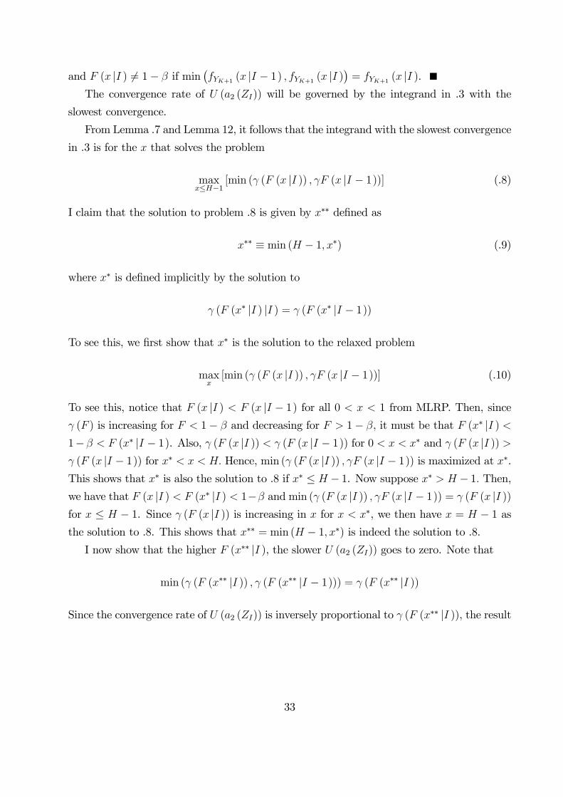
maxx≤H−1
[min (γ (F (x |I )) , γF (x |I − 1))] (.8)
I claim that the solution to problem .8 is given by x∗∗ defined as
x∗∗ ≡ min (H − 1, x∗) (.9)
where x∗ is defined implicitly by the solution to
γ (F (x∗ |I ) |I ) = γ (F (x∗ |I − 1))
To see this, we first show that x∗ is the solution to the relaxed problem
maxx[min (γ (F (x |I )) , γF (x |I − 1))] (.10)
To see this, notice that F (x |I ) < F (x |I − 1) for all 0 < x < 1 from MLRP. Then, since
γ (F ) is increasing for F < 1− β and decreasing for F > 1− β, it must be that F (x∗ |I ) <1−β < F (x∗ |I − 1). Also, γ (F (x |I )) < γ (F (x |I − 1)) for 0 < x < x∗ and γ (F (x |I )) >γ (F (x |I − 1)) for x∗ < x < H. Hence, min (γ (F (x |I )) , γF (x |I − 1)) is maximized at x∗.This shows that x∗ is also the solution to .8 if x∗ ≤ H − 1. Now suppose x∗ > H − 1. Then,we have that F (x |I ) < F (x∗ |I ) < 1−β and min (γ (F (x |I )) , γF (x |I − 1)) = γ (F (x |I ))for x ≤ H − 1. Since γ (F (x |I )) is increasing in x for x < x∗, we then have x = H − 1 asthe solution to .8. This shows that x∗∗ = min (H − 1, x∗) is indeed the solution to .8.I now show that the higher F (x∗∗ |I ), the slower U (a2 (ZI)) goes to zero. Note that
Since the convergence rate of U (a2 (ZI)) is inversely proportional to γ (F (x∗∗ |I )), the result
33
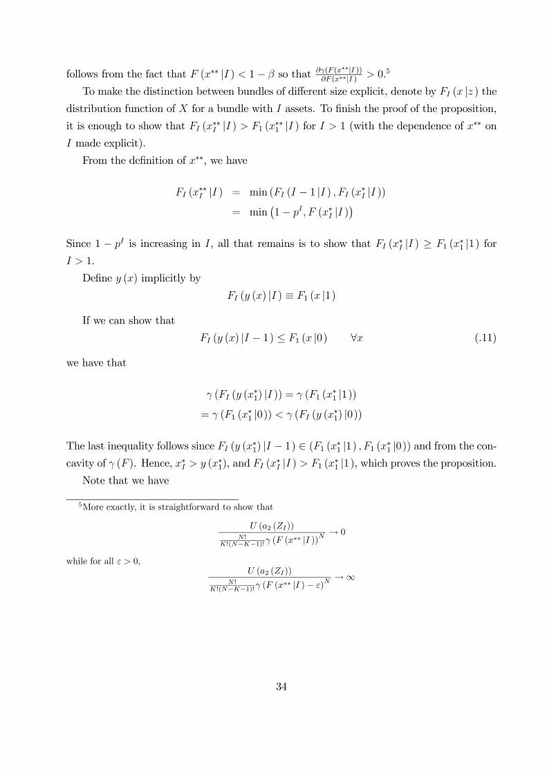
follows from the fact that F (x∗∗ |I ) < 1− β so that ∂γ(F (x∗∗|I ))∂F (x∗∗|I ) > 0.5
To make the distinction between bundles of different size explicit, denote by FI (x |z ) thedistribution function of X for a bundle with I assets. To finish the proof of the proposition,
it is enough to show that FI (x∗∗I |I ) > F1 (x
∗∗1 |I ) for I > 1 (with the dependence of x∗∗ on
I made explicit).
From the definition of x∗∗, we have
FI (x∗∗I |I ) = min (FI (I − 1 |I ) , FI (x
∗I |I ))
= min¡1− pI , F (x∗I |I )
¢Since 1 − pI is increasing in I, all that remains is to show that FI (x
∗I |I ) ≥ F1 (x
∗1 |1) for
I > 1.
Define y (x) implicitly by
FI (y (x) |I ) ≡ F1 (x |1)
If we can show that
FI (y (x) |I − 1) ≤ F1 (x |0) ∀x (.11)
we have that
γ (FI (y (x∗1) |I )) = γ (F1 (x
∗1 |1))
= γ (F1 (x∗1 |0)) < γ (FI (y (x
∗1) |0))
The last inequality follows since FI (y (x∗1) |I − 1) ∈ (F1 (x∗1 |1) , F1 (x∗1 |0)) and from the con-
cavity of γ (F ). Hence, x∗I > y (x∗1), and FI (x∗I |I ) > F1 (x
∗1 |1), which proves the proposition.
Note that we have
5More exactly, it is straightforward to show that
U (a2 (ZI))N !
K!(N−K−1)!γ (F (x∗∗ |I ))N
→ 0
while for all ε > 0,U (a2 (ZI))
N !K!(N−K−1)!γ (F (x
∗∗ |I )− ε)N→∞
34
f1 (0 |0)f1 (0 |1)
=1− q
1− p
f1 (1 |0)f1 (1 |1)
=q
p
and
fI (x |I − 1)fI (x |I )
=
I−1!(J−1)!(I−J)! (1− p)I−J pJ−1q + I−1!
J!(I−J−1)! (1− p)I−J−1 pJ (1− q)
I!J !(I−J)! (1− p)I−J pJ
=J
I
q
p+
I − J
I
1− q
1− p
where J is an integer such that J ≤ x < J+1. Therefore, we have f1(0|0)f1(0|1) ≥
fI(y|I−1 )fI(y|I ) ≥
f1(1|0)f1(1|1)
for all y. This implies inequality .11, since for x < 1, we have
f1 (x |0)f1 (x |1)
≥ fI (y |I − 1)fI (y |I )
⇒
F1 (x |0) fI (y |I ) ≥ F1 (x |1) fI (y |I − 1)⇒
F1 (x |0)FI (y |I ) ≥ F1 (x |1)FI (y |I − 1)⇒
F1 (x |0) ≥ FI (y (x) |I − 1)
Similarly, for x ≥ 1,
f (x |0)f (x |1) ≤
f (y |I − 1)f (y |I ) ⇒
(1− F1 (x |0)) fI (y |I ) ≤ (1− F1 (x |1)) fI (y |I − 1)⇒
(1− F1 (x |0)) (1− FI (y |I )) ≤ (1− F1 (x |1)) (1− FI (y |I − 1))⇒
fYK+2:N ,YK+1,YK (Y, x, x |I )fYK+2:N ,YK+1 (Y, x)
fYK+2:N ,YK+1,YK (Y, x, x)dY dx
= P (I)
Z H
0
fYK+1 (x |I ) dx
−P (I)Z H
0
ZYK+2:N
C
D
f (x |I )1− F (x |I )fYK+2:N ,YK+1 (Y, x |I )
fYK+2:N ,YK+1 (Y, x)
fYK+2:N ,YK+1,YK (Y, x, x)dY dx
= P (I)
Z H
0
fYK+1 (x |I ) dx
−P (I)Z H
0
fYK+1 (x |I )ZYK+2:N
C
D
f (x |I )1− F (x |I )fYK+2:N (Y |I, YK+1 = x)
fYK+2:N ,YK+1 (Y, x)
fYK+2:N ,YK+1,YK (Y, x, x)dY dx
= P (I)
Z H
0
fYK+1 (x |I ) dx
−P (I)Z H
0
fYK+1 (x |I )ZYK+2:N
fYK+2:N (Y |I, YK+1 = x)
CD
f(x|I )1−F (x|I )fYK+2:N ,YK+1 (Y, x)P
zCD
f(x|z )1−F (x|z )fYK+2:N ,YK+1 (Y, x |z )P (z)
dY dx
= P (I)
Z H
0
fYK+1 (x |I ) dx
−P (I)Z H
0
fYK+1 (x |I )ZYK+2:N
f(x|I )1−F (x|I )P
zf(x|z )
1−F (x|z )fYK+2:N,YK+1
(Y,x|z )fYK+2:N,YK+1
(Y,x)P (z)
fYK+2:N (Y |I, YK+1 = x) dY dx
= P (I)
Z H−1
0
fYK+1 (x |I )A (x)
−P (I)Z H
0
fYK+1 (x |I )ZYK+2:N
f(x|I )1−F (x|I )P
zf(x|z )
1−F (x|z )fYK+2:N,YK+1
(Y,x|z )fYK+2:N,YK+1
(Y,x)P (z)
fYK+2:N (Y |I, YK+1 = x) dY dx
= P (I)
Z H−1
0
fYK+1 (x |I )A (x) .
We need to show that for a cut off level P ∗1 where A (x) converges for one asset, it does not
36
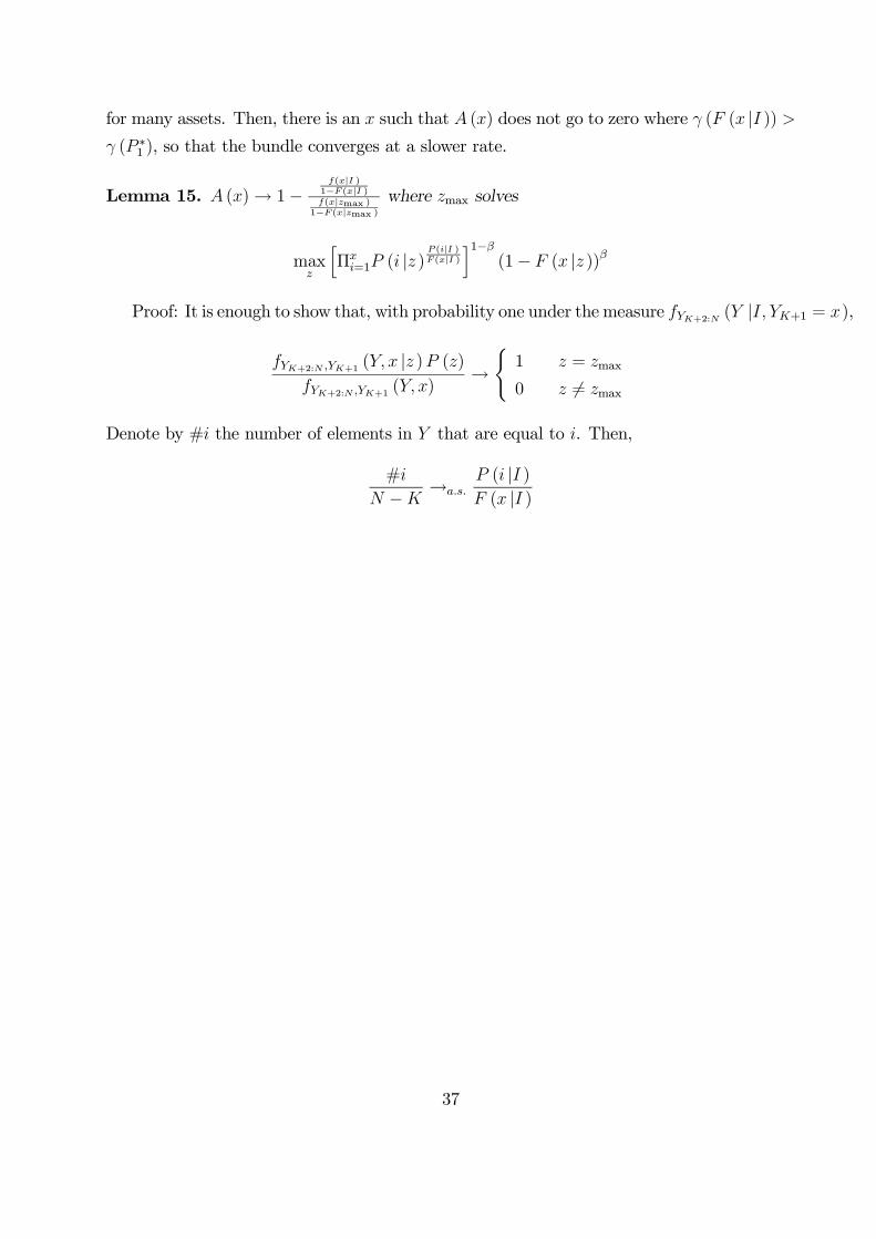
for many assets. Then, there is an x such that A (x) does not go to zero where γ (F (x |I )) >γ (P ∗1 ), so that the bundle converges at a slower rate.
Lemma 15. A (x)→ 1−f(x|I )
1−F (x|I )f(x|zmax )
1−F (x|zmax )where zmax solves
maxz
hΠxi=1P (i |z )
P (i|I )F (x|I )
i1−β(1− F (x |z ))β
Proof: It is enough to show that, with probability one under the measure fYK+2:N (Y |I, YK+1 = x),
fYK+2:N ,YK+1 (Y, x |z )P (z)fYK+2:N ,YK+1 (Y, x)
→(1 z = zmax
0 z 6= zmax
Denote by #i the number of elements in Y that are equal to i. Then,
#i
N −K→a.s.
P (i |I )F (x |I )
37
under the measure fYK+2:N (Y |I, YK+1 = x) for i ≤ x. We have that
fYK+2:N ,YK+1 (Y, x |z )P (z)fYK+2:N ,YK+1 (Y, x)
=
³Πxi=0P (i |z )
#iN−K−1
´N−K−1P (x |z ) (1− F (x |z ))K P (z)P
u
³Πxi=0P (i |u)
#iN−K−1
´N−K−1P (x |u) (1− F (x |u))K P (u)
=
ÃΠxi=0P (i|z )
#iN−K−1
Πxi=1P (i|zmax )
P (i|I )F (x|I )
!N−K−1
P (x |z )³
1−F (x|z )1−F (x|zmax )
´KP (z)
Pu
ÃΠxi=0P (i|u )
#iN−K−1
Πxi=1P (i|zmax )P (i|I )F (x|I )
!N−K−1
P (x |u)³
1−F (x|u )1−F (x|zmax )
´KP (u)
=
ÃΠxi=0P (i|z )
#iN−K−1
Πxi=1P (i|zmax )
P (i|I )F (x|I )
!N((1−β)− 1N ) ³
1−F (x|z )1−F (x|zmax )
´Nβ
P (x |z )P (z)
Pu
ÃΠxi=0P (i|u )
#iN−K−1
Πxi=1P (i|zmax )P (i|I )F (x|I )
!N((1−β)− 1N ) ³
1−F (x|u )1−F (x|zmax )
´Nβ
P (x |u)P (u)
=
⎡⎣Ã Πxi=0P (i|z )#i
N−K−1
Πxi=1P (i|zmax )
P (i|I )F (x|I )
!(1−β)− 1N ³
1−F (x|z )1−F (x|zmax )
´β⎤⎦N P (x |z )P (z)
Pu
⎡⎣Ã Πxi=0P (i|u )
#iN−K−1
Πxi=1P (i|zmax )
P (i|I )F (x|I )
!((1−β)− 1N ) ³
1−F (x|u )1−F (x|zmax )
´β⎤⎦N P (x |u)P (u)
Here, for a set of measure one, if z 6= zmax,ÃΠxi=0P (i |z )
#iN−K−1
Πxi=1P (i |zmax )
P (i|I )F (x|I )
!(1−β)− 1N µ
1− F (x |z )1− F (x |zmax )
¶β
→ C < 1
And hence the result follows. Hence, A (x) goes to zero for x such that zmax < I.∙Πxi=1f (yi |I )
f(yi|I )F (x|I )
¸1−β(1− F (x |I ))β =
∙Πxi=1 (f (yi |I − 1))
f(yi|I )F (x|I )
¸1−β(1− F (x |I − 1))β
We can rewrite this as⎡⎣Πxi=1
f (yi |I − 1)f (yi |I )
f(yi|I )F (x|I )
⎤⎦1−β µ1− F (x |I − 1)1− F (x |I )
¶β
= 1
38
(1− β)XJ≤x
f (J |I )F (x |I ) ln
µJ
I
q
p+
I − J
I
1− q
1− p
¶+ β ln
XJ>x
f (J |I )1− F (x |I )
µJ
I
q
p+
I − J
I
1− q
1− p
¶= 0
(1− β)E
µln
µJ
I
q
p+
I − J
I
1− q
1− p
¶|J ≤ x, I
¶+ β lnE
µJ
I
q
p+
I − J
I
1− q
1− p|J > x, I
¶= 0
Denote by L (x) the function x qp+ (1− x) 1−q
1−p . Then, we can rewrite this as
(1− β)E
µln
µL
µX
I
¶¶|X ≤ x, I
¶+ β lnE (L (J) |J > x, I ) = 0
We know that
F (x |I )EµJ
I
q
p+
I − J
I
1− q
1− p|J ≤ x, I
¶+(1− F (x |I ))E
µJ
I
q
p+
I − J
I
1− q
1− p|J > x, I
¶=
E
µJ
I
q
p+
I − J
I
1− q
1− p|I
=
qpE (J) + 1−q
1−pE (I − J)
I=
q
pp+
1− q
1− p(1− p) = 1,
or
ln
∙F (x |I )E
µJ
I
q
p+
I − J
I
1− q
1− p|J ≤ x, I
¶+ (1− F (x |I ))E
µJ
I
q
p+
I − J
I
1− q
1− p|J > x, I
¶¸= 0.
Then, from Jensen’s inequality, we have
F (x |I ) lnEµJ
I
q
p+
I − J
I
1− q
1− p|J ≤ x, I
¶+
+(1− F (x |I )) lnEµJ
I
q
p+
I − J
I
1− q
1− p|J > x, I
¶< 0
F (x |I )Eµln
µJ
I
q
p+
I − J
I
1− q
1− p
¶|J ≤ x, I
¶+
+(1− F (x |I )) lnEµJ
I
q
p+
I − J
I
1− q
1− p|J > x, I
¶< 0
Both these follow from Jensen’s inequality: E (f (x)) < f (E (x)) for f a concave function.
39
Also, we have
E
µln
µJ
I
q
p+
I − J
I
1− q
1− p
¶|J ≤ x, I
¶> lnE
µJ
I
q
p+
I − J
I
1− q
1− p|J > x, I
¶Hence, we have to have
1− β > F (x |I )
Now, let I grow. Then, f¡JI
¢goes to a peaked distribution around p. Since
√I
µJ
I
q
p+
I − J
I
1− q
1− p− 1¶→ N (0, 1)
we have that
√I ln
µJ
I
q
p+
I − J
I
1− q
1− p
¶→ N (0, 1)
so that
E
µ√I ln
µJ
I
q
p+
I − J
I
1− q
1− p
¶|J ≤ x, I
¶→ E
µ√I
µJ
I
q
p+
I − J
I
1− q
1− p− 1¶|J ≤ x, I
¶and
√I lnE
µJ
I
q
p+
I − J
I
1− q
1− p|J > x, I
¶→ E
µ√I
µJ
I
q
p+
I − J
I
1− q
1− p− 1¶|J > x, I
(1− β)E
µ√I ln
µJ
I
q
p+
I − J
I
1− q
1− p
¶|J ≤ x, I
¶+β√I lnE
µJ
I
q
p+
I − J
I
1− q
1− p|J > x, I
¶= 0
Show that
F (x |I )→ 1− β
40
We have that √I
µJ
I− p
¶→ N (0, p(1− p))
and √I
µJ
I
q
p+
I − J
I
1− q
1− p− 1¶→ N
¡0, σ2
¢Also,
√I ln
µJ
I
q
p+
I − J
I
1− q
1− p
¶∼√I
µJ
I
q
p+
I − J
I
1− q
1− p− 1
and
E
µ√I ln
µJ
I
q
p+
I − J
I
1− q
1− p
¶|J ≤ x, I
¶→ E
µ√I
µJ
I
q
p+
I − J
I
1− q
1− p− 1¶|J ≤ x, I
¶√I lnE
µJ
I
q
p+
I − J
I
1− q
1− p|J > x, I
¶→√IE
µµJ
I
q
p+
I − J
I
1− q
1− p− 1¶|J > x, I
¶Therefore, there exists I such that
which shows that the cut-off level is increasing in I. Hence, at the F (x |I ) where wehave convergence for one asset, there is no convergence of A (y (x)) for many assets, and we
can increase F (x |I ) slightly and hence γ (F (x |I )) .Also, since
E
µln
µJ
I
q
p+
I − J
I
1− q
1− p
¶|J ≤ x, I
¶< lnE
µJ
I
q
p+
I − J
I
1− q
1− p|J ≤ x, I
¶It has to be that the cut off level for ascending price auctions is in general lower than for