Bundling Time and Goods: Implications for Hours Dispersion Lei Fang, Anne Hannusch, and Pedro Silos * January 9, 2020 Abstract We document the large dispersion in hours worked in the cross-section. We ac- count for this fact using a model in which households combine market inputs and time to produce a set of non-market activities. To estimate the model, we create a novel data set that pairs market expenditures and time use at the activ- ity level using data from the Consumer Expenditure Survey and the American Time Use Survey, respectively. The estimated model can account for a large fraction of the dispersion of hours worked in the data. The substitutability be- tween market inputs and time within an activity and across a sizable number of activities is key to our results. We show that models that lack these features can only generate one-third of the observed hours dispersion. JEL Codes: J22, E21, D11 Keywords: Time Allocation, Consumption Expenditures, Hours Dispersion, Elasticity of Substitution * Affiliation: Federal Reserve Bank of Atlanta (Fang), University of Mannheim (Hannusch), and Temple University (Silos). We thank audiences at various conferences and universities for useful comments. We want to especially thank Yongsung Chang, Nicola Fuchs-Schündeln, Nezih Guner, Karen Kopecky, Dirk Krueger, Rachel Ngai, B. Ravikumar, Richard Rogerson, Chris Tonetti, and Gianluca Violante for feedback at all stages of this project. The views represented here are those of the authors and they do not represent the views of the Federal Reserve Bank of Atlanta, the Federal Reserve System or its Board of Governors. Hannusch gratefully acknowledges financial support by the German Research Foundation (DFG) through CRC TR 224 (project A03).
Transcript
Bundling Time and Goods: Implications forHours Dispersion
Lei Fang, Anne Hannusch, and Pedro Silos∗
January 9, 2020
Abstract
We document the large dispersion in hours worked in the cross-section. We ac-count for this fact using a model in which households combine market inputsand time to produce a set of non-market activities. To estimate the model, wecreate a novel data set that pairs market expenditures and time use at the activ-ity level using data from the Consumer Expenditure Survey and the AmericanTime Use Survey, respectively. The estimated model can account for a largefraction of the dispersion of hours worked in the data. The substitutability be-tween market inputs and time within an activity and across a sizable numberof activities is key to our results. We show that models that lack these featurescan only generate one-third of the observed hours dispersion.
JEL Codes: J22, E21, D11Keywords: Time Allocation, Consumption Expenditures, Hours Dispersion,Elasticity of Substitution
∗Affiliation: Federal Reserve Bank of Atlanta (Fang), University of Mannheim (Hannusch), and Temple University(Silos). We thank audiences at various conferences and universities for useful comments. We want to especially thankYongsung Chang, Nicola Fuchs-Schündeln, Nezih Guner, Karen Kopecky, Dirk Krueger, Rachel Ngai, B. Ravikumar, RichardRogerson, Chris Tonetti, and Gianluca Violante for feedback at all stages of this project. The views represented here arethose of the authors and they do not represent the views of the Federal Reserve Bank of Atlanta, the Federal Reserve Systemor its Board of Governors. Hannusch gratefully acknowledges financial support by the German Research Foundation (DFG)through CRC TR 224 (project A03).
1 Introduction
The dispersion of market hours across workers is large. The literature thus far has
relied on unobserved tastes for leisure to generate the hours dispersion that we
observe in the data.1 Explaining hours dispersion instead as a result of observables
improves our understanding of the earnings distribution, which is an essential
ingredient in analyzing questions in macroeconomics, labor economics, and public
finance.
This paper proposes a model that generates large dispersion in hours worked
in the absence of preference heterogeneity and is consistent with the rich cross-
sectional patterns of time use and expenditures. In the model, households com-
bine time and market inputs (goods and services) to enjoy non-market activities.
Throughout the paper, we define non-market activities as activities related to home
production and leisure. One example of such an activity is a restaurant meal. It re-
quires the purchase of market goods and services, combined with a person’s own
time to enjoy utility from restaurant meals; such utility cannot be enjoyed without
both inputs. This idea goes back to Becker (1965), and while it forms the basis of
the home production literature, we generalize the idea to include all non-market
activities households engage in. Our innovation is to divide non-market hours
into time segments, in which each segment is paired with specific market inputs
to produce an activity.
The observed heterogeneity we rely on to explain hours dispersion is the het-
erogeneity in wages. In our model, the response of hours worked to wage changes
depends on the substitutability between market inputs and time within an activ-
ity and across activities. Hence, to what extent wage dispersion translates into
hours dispersion depends on the magnitude of these two types of elasticities of
substitution and, ultimately, remains a quantitative question.
Estimating the model inspired by Becker (1965) is challenging, as it requires
data on time use and market inputs bundled at the activity level. Our first contri-
bution is to create a novel data set that maps time-use categories from the Amer-
1See, for example, Kaplan (2012) or Heathcote et al. (2014).
2
ican Time Use Survey (ATUS) and market input categories from the Consumer
Expenditure Survey (CEX) into a common set of activities. Our reference is the
set of activities proposed by Aguiar et al. (2013), who classify time-use data into
market work, child care, non-market work (home production), and several leisure
categories. We take these categories as given and map market input expenditures
into these time-use categories. By averaging time and expenditures for households
belonging to the same educational group in a given year, we construct a pseudo-
panel of household allocations over the sample period 2003-2014.
From this newly created data set, we document substantial heterogeneity in
the time and expenditure bundles allocated to different activities. Market work
requires hardly any expenditures and varies mostly along the time dimension.
Highly educated households spend significantly more time working in the market.
Non-market work activities, on the other hand, are mostly heterogeneous in terms
of the expenditures allocated to them. Less educated households spend a much
larger fraction of their budget on these activities. Finally, leisure activities stand
out. They exhibit heterogeneity along both dimensions of time and expenditure.
Highly educated households allocate less time to leisure, but they spend a larger
fraction of their budget on these activities. Despite overall lower leisure hours,
more educated households devote more time to leisure activities that require more
expenditures, such as dining out and vacations. Less educated households, in
contrast, spend more time on leisure activities that require lower expenditures,
such as watching TV.
We supplement the pseudo-panel of time and expenditure bundles with data
on wages and prices to estimate the model. The form of preferences we take to
the data is of the nested constant elasticity of substitution (CES) type. The utility
from each activity is a CES aggregator of market inputs and time. We estimate
the elasticities of substitution between market inputs and time for a set of six non-
market activities, as well as the elasticity of substitution across these activities.
We find that one can substitute market inputs with time quite easily for a given
activity and that activities themselves are substitutable, but to a lesser extent.
We simulate the model and show that it accounts for 55% of the dispersion
3
in market hours over the sample period. The only source of heterogeneity in the
model stems from the cross-sectional distribution of wages, which we take from
the Current Population Survey. Two model innovations account for this result: (1)
the division of non-market time into activity-specific segments and (2) the inclu-
sion of a sizable number of non-market activities. The estimation suggests a high
degree of substitutability between market inputs and time within most activities
as well as across activities. This empirical finding, in combination with the two
model innovations, implies that time allocation choices are much more sensitive
to wage changes: Households not only reallocate market inputs and non-market
time within a given activity but also across a large set of activities. These addi-
tional margins of adjustment imply large responses of market hours to changes in
wages.
We estimate several alternative utility specifications using the same data to ex-
plore the importance of the two model innovations. To disentangle the importance
of the first innovation, we estimate a form of CES utility that includes the same
number of market inputs but lumps all non-market time together in the standard
notion of leisure. This model can only account for 29% of the dispersion in hours
worked. To capture the importance of the second innovation, we estimate the same
model but reduce the number of activities from six to two. This model can only
account for 32% of the dispersion in hours worked.
Related Literature This paper contributes to a large and growing literature on
home production and leisure production.2 More specifically, it generalizes the
idea of home or leisure production and fully exploits the heterogeneity in the
household production of consumption activities outside the market. We argue that
such a generalization is crucial to understanding the cross-sectional dispersion in
hours worked.
This paper also relates to the literature on time allocation. The most prominent
example is Aguiar and Hurst (2007b), who document trends in time allocated to
market work, non-market work, and leisure. A more recent paper, Aguiar et al.
2See, for example, Benhabib et al. (1991), Greenwood and Hercowitz (1991), McGrattan et al.(1997), Vandenbroucke (2009), Kopecky (2011), Ngai and Pissarides (2011), Bridgman (2016), Fangand Zhu (2017), Ngai and Petrongolo (2017) and Bopphart and Ngai (2019).
4
(2019), finds that innovations in recreational computing technology can account
for a large fraction of the decline in young men’s labor supply since 2004. We con-
tribute to this literature by mapping time use categories to expenditure categories.
This mapping allows us to study how bundles of time and market inputs differ
across a wide set of non-market activities and household types. More recently,
Boerma and Karabarbounis (2019a) and Boerma and Karabarbounis (2019b) study
welfare inequality using an alternative approach to obtain time and expenditures
for home and leisure production. They impute levels of time use for households in
the CEX using variables that are common to the CEX and the ATUS. The mapping
we propose does not rely on any imputation, and we present expenditures and
time use for a much larger set of activities.
Finally, this paper relates to the macroeconomic literature that studies inequal-
ity (e.g. Heathcote et al. (2014) and Kaplan (2012)), unemployment (Bils et al.
(2012)), and the relationship between wealth and labor supply heterogeneity (Mus-
tre del Rio (2015)). These papers rely on ex ante heterogeneity in preferences for
leisure to generate dispersion in hours worked. The model presented in this pa-
per, in contrast, does not rely on preference heterogeneity. It generates dispersion
in hours only through heterogeneity in wages, which is observable and relatively
well measured.
The rest of the paper is organized as follows. Section 2 presents data facts on
the dispersion in hours worked and bundles of time use and market inputs across
different activities. Section 3 presents the model. Section 4 discusses the estimation
strategy and estimation results. Section 5 uses the estimated models to understand
the effects of wage dispersion on hours dispersion. Section 6 concludes.
2 Data
We begin by documenting the large dispersion in hours worked within and across
education groups. We argue that this dispersion may reflect heterogeneity in
household choices outside the market. To this end, we provide evidence that bun-
dles of market inputs and time for non-market activities vary by education level.
5
We group households into four education categories: (1) less than high school, (2)
high school, (3) some college, and (4) college and above.
2.1 Dispersion of Hours Worked
We measure dispersion of hours worked as the standard deviation of log usual
hours worked in the Current Population Survey Outgoing Rotation Group (CPS-
ORG) between 2003 and 2014. We restrict the sample to individuals between the
ages of 21 and 65. Table 1 summarizes the results across all years and for two sub-
periods: 2003-2007 and 2008-2014. Dispersion in hours worked is slightly higher
for more educated individuals and increased somewhat during and after the Great
Recession. However, the variation across education groups and across time periods
is relatively small. Hence, we use the average dispersion over the entire sample
period as the benchmark for our analysis.
Table 1: Dispersion in Hours Worked
2003-2014 2003-2007 2008-2014
Less than HS 0.402 0.380 0.419High School 0.397 0.385 0.405Some College 0.445 0.439 0.449College 0.464 0.469 0.460
Total 0.435 0.428 0.440Data Source: IPUMS-CPS Outgoing Rotation Group 2003-2014. The
sample is restricted to workers aged 21-65. Dispersion of hoursworked is measured as the standard deviation of log usual hoursworked per week. If usual hours worked per week is not available,we use information on actual hours worked.
2.2 Time and Expenditure Allocations
2.2.1 Data Construction
To the best of our knowledge, no single data source includes bundles of expen-
ditures and time use for a broad set of activities. Hence, we use the Consumer
Expenditure Survey (CEX) for data on market inputs and combine it with time
use data from the American Time Use Survey (ATUS) at the activity level. We re-
strict both samples to reference persons between the ages of 21 and 65. We remove
students and retirees, since we do not model education or retirement decisions. Be-
6
cause our main focus is the dispersion of market hours, we also restrict the sample
to households with working individuals. The sample period is 2003-2014.
Our first contribution is to develop a mapping that consistently links market
input expenditures to time use at the activity level. We take the time use classifi-
cation of Aguiar and Hurst (2007b), Aguiar et al. (2012) and Aguiar et al. (2019)
as our starting point. Matching expenditures to these time use categories involves
two steps. First, we create a baseline match between both surveys using the ag-
gregated consumption expenditure categories provided by the Bureau of Labor
Statistics. We then check the detailed expenditure series underlying these major
categories. If necessary, we reassign expenditure subseries to different time use
categories in order to maintain a consistent mapping. The details of the data con-
struction process are described in Appendix A.
Some expenditures cannot be directly linked to a specific activity; these mainly
constitute investment decisions. For example, the purchase of a house or car is not
only a consumption decision but also an investment decision.3 Similarly, expen-
ditures spent on education and medical care are part of the investment in human
capital.4 Given the static framework presented in this paper, we choose to exclude
all investment expenditures from our main analysis. In addition, expenditures on
transportation, such as gas, maintenance of a vehicle, public transportation, etc.,
cannot be separated into direct transportation costs associated with actual activ-
ities. We therefore also exclude these from our analysis. We refer to the set of
expenditures included in our analysis as “core expenditures.” Between 2003 and
2014, core expenditures constitute slightly more than half of total consumption
expenditures reported in the CEX.
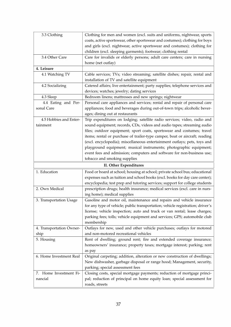
Our proposed mapping between time use and expenditures leads to four main
activity categories: market work, non-market work, child care, and leisure, where
non-market work is mostly home production. Leisure itself can be divided into five
subcategories: watching TV, sleep, socializing, eating out and personal care, and
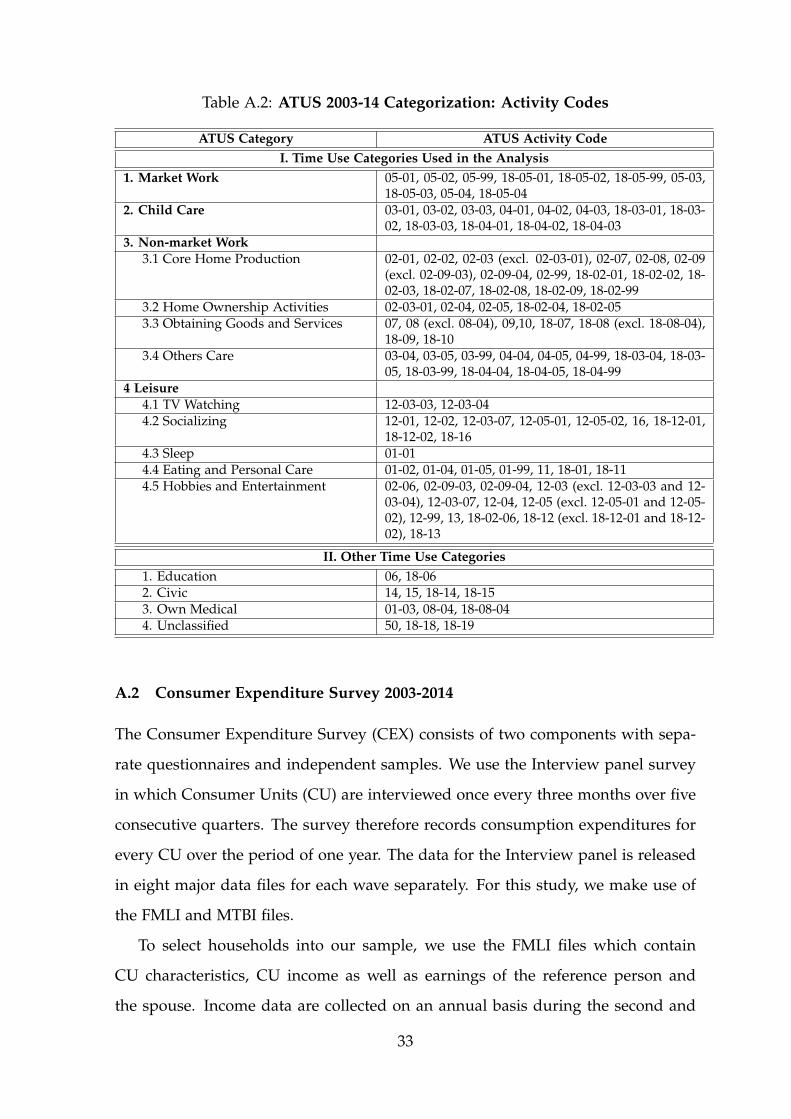
hobbies and entertainment. Please refer to Tables A.1-A.4 for a detailed description
3The maintenance costs of a house are included in non-market work.4For consistency, we also exclude time spent on education and medical care from the analysis.
7
of these categories.
2.2.2 Stylized Facts
Figure 1 documents substantial heterogeneity by education in the time and expen-
diture bundles allocated to each of the four main activities. Time spent on each
activity is reported in weekly hours and plotted on the x-axis. Expenditures for
market inputs allocated to the same activity are shown on the y-axis and reported
as a fraction of core expenditures. Households are grouped by educational attain-
ment, with group 1 having the lowest attainment. We report average allocations
over the entire sample period as time and expenditure shares vary little over time.
Notes: Households are grouped into four education groups: 1 - less than high school, 2 - high school, 3 - some college, 4- college and above. Consumption expenditures are expressed as a fraction of core expenditures. Time use is reported asweekly hours.
First, market work requires hardly any expenditures at the household level,
but varies tremendously in terms of time allocation. College-educated households
Notes: Households are grouped into four education groups: 1 - less than high school, 2 - high school, 3 - some college, 4- college and above. Consumption expenditures are expressed as a fraction of core expenditures. Time use is reported asweekly hours.
spend roughly 12 hours more per week working in the market compared to high
school dropouts. The opposite is true for non-market work. Time allocated to non-
market work varies little by education. Yet, non-market work activities constitute
one-half to two-thirds of core expenditures. The expenditure share is declining in
education, with high school dropouts allocating 12 percentage points more of their
budget to non-market work activities relative to college graduates. Expenditures
on child care are increasing in education, while weekly hours spent on child care
are U-shaped.
The time and expenditure bundles for leisure activities follow a strikingly dif-
ferent pattern. These bundles vary along both dimensions with educational attain-
ment. Expenditure shares for leisure activities are increasing in education, while
time use is decreasing. For example, high school dropouts enjoy 11 more leisure
hours per week than college graduates, which roughly mirrors the difference in
market hours. Meanwhile, high school dropouts spend 11 percentage points less
of their expenditures on leisure activities.
To understand what drives the pattern of time and expenditure bundles for
9
leisure, we decompose leisure activities into five subcategories. Figure 2 plots time
use and expenditure shares for these subcategories. Sleep and watching TV are
the two leisure activities that absorb the majority of leisure time. The difference in
leisure hours by education is mainly driven by these two activities. High school
dropouts spend 10 hours more per week watching TV and 7 hours more sleeping
than college graduates. Both activities are associated with hardly any expendi-
tures.
Hobbies and entertainment and eating out and personal care, are the two
leisure activities that dominate household expenditures. These activities drive the
increase in leisure expenditure shares by education. College graduates spend 12
percentage points more of their core expenditures on both categories compared
with high school dropouts. Although college graduates overall spend less time
on leisure, they allocate 6 hours more per week between hobbies and entertain-
ment and eating out and personal care. Taken together, these facts rationalize why
more educated households spend less time but a larger fraction of their budget on
leisure activities.
We perform several checks to demonstrate the robustness of these stylized facts.
First, we split the 2003-2014 sample into two subperiods, 2003-2007 and 2008-2014.
The cross-sectional time and expenditure allocations look similar for the two sub-
samples.5 Next, instead of grouping households by education, we split them by
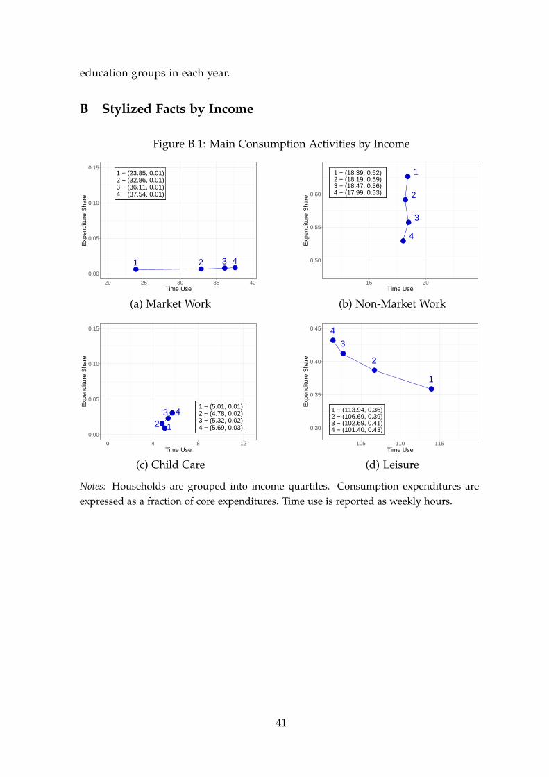
income quartiles. Figures B.1 and B.2 in the Appendix show the results when we
split households along income quartiles. Even though all results go through, we
lose a nontrivial number of observations due to the fact that the household income
variable in the ATUS contains a lot of missing observations. Hence, we choose to
continue the analysis with the education classification.
3 Structural Framework
3.1 The Model
Becker (1965) emphasizes that different types of time use and different types of
5Figures showing activity bundles for each subperiod are available upon request.
10
market inputs can be combined in various ways to provide utility. Hence, his no-
tion of utility is far more general than the standard assumption in the macroeco-
nomics literature, in which total non-market time is often combined into a general
notion of leisure time.
We formalize Becker’s (1965) notion in a nested CES production function. House-
holds combine time li and market inputs xi in a CES production function to pro-
duce consumption of activity i, denoted by ci. Household utility is defined over
the combination of all activities and aggregated using CES preferences:
u(ci) = log
{(∑
iαic
ρ−1ρ
i
) ρρ−1}
, ci =
(κix
ξi−1ξi
i + (1− κi)`ξi−1
ξii
) ξiξi−1
with 0 ≤ α ≤ 1, 0 ≤ κ ≤ 1, ρ ≥ 0, and ξi ≥ 0. Four sets of parameters govern
the utility function. First, αi determines the relative weights of every activity in
the overall set of activities. Second, ρ captures the elasticity of substitution be-
tween these consumption activities. Third, for a given activity i, κi determines the
weight of market inputs in the production of every activity. Finally, the elasticity
of substitution between market inputs and time is given by ξi. ξi can vary across
activities, implying that the extent to which households substitute between market
inputs and their own time may differ across activities. This parsimonious way of
modeling the production of activities yields a flexible arrangement in which time
use and market inputs are combined.
Section 2 documents that consumption expenditures related to market work are
virtually zero. Hence, we assume that market work does not require consumption
expenditures. Each household has one unit of time that can be allocated to the
production of non-market activities or market work. Let w be the wage rate and
pi the price of market input xi associated with activity i. The budget constraint is
∑i
pixi = w(1−∑i`i).
Two model innovations distinguish our framework from more commonly used
macroeconomic models and thus warrant further discussion. The first innova-
tion is that non-market time—the standard notion of leisure—is divided into sev-
11
eral time segments and each segment is linked to the production of one activity.
Hence, we depart from the standard assumption that all leisure hours are perfect
substitutes. If leisure hours are imperfect substitutes, households care about the
allocation of time segments to activities instead of the total time spent on leisure.
The effect of this assumption is summarized by the optimal ratio of time to market
inputs for activity i:`i
xi=( pi
w
)ξi(
1− κi
κi
)ξi
. (1)
Because ξi ≥ 0 ∀i, an increase in wages leads to a decline in the input ratio`ixi
. The intuition is simple: Wage increases induce more market work and thus a
reduction in non-market time `i spent on producing activity i. At the same time,
the increase in income enables households to purchase additional market inputs
xi. As a result, households substitute market inputs for time. The magnitude of
the substitution is governed by ξi. Since ξi is activity-specific, so is the response of`ixi
to wage increases. A higher elasticity, ξi, implies that time and market inputs are
more substitutable, resulting in larger decreases in the non-market time segment
`i and therefore a larger increase in market hours.
The second model innovation is the introduction of a large set of non-market
activities. We depart from the common assumption in the home production and
leisure production literature that all market inputs and non-market time engaged
in home or leisure production are perfectly substitutable. For instance, these mod-
els assume that cable services are a perfect substitute for restaurant services and
that time spent on watching TV can be perfectly substituted for time spent din-
ing out. In contrast, the model inspired by Becker (1965) interprets watching TV
and eating in a restaurant as two distinct activities that follow separate production
processes. The second model innovation allows households to substitute among a
larger set of activities. The quantitative effect of this channel on the allocation of
time and market inputs is governed by the substitution parameter ρ.
Both model innovations are important for generating dispersion in hours worked.
To demonstrate this point, we contrast the responsiveness of hours worked to wage
changes in the model à la Becker (1965) with several model versions that lack either
12
one or both model innovations. For ease of notation, we call the model presented
in this section the Becker model.
3.2 Relaxing Both Model Innovations
We begin by presenting a model version that relaxes both model innovations. This
takes us back to the most prevalent form of utility in the literature, which is why
we refer to it as the Standard model. Households derive utility from total market
consumption and enjoy total leisure time. To be consistent with the model laid out
in the previous section, the utility function is given by a CES aggregator between
consumption xs and leisure `s:
u(xs, `s) = log
{(φs(xs)
σs−1σs + (1− φs)(`s)
σs−1σs
) σsσs−1}
where σs ≥ 0 is the elasticity of substitution between consumption and leisure.
After normalizing the price of consumption to one, the budget constraint is:
xs = w(1− `s).
In the Standard model, the optimal allocation between time and market con-
sumption is summarized by
`s
xs =
(1w
)σs (1− φs
φs
)σs
(2)
The response of `s
xs to a wage change is determined by the elasticity parameter σs,
which has a similar role as ξi in the Becker model. The difference is that wage
changes can now only influence the substitution between total consumption and
total leisure. Hence, the effects of substituting between market inputs and time
within an activity, as well as across activities, are both muted in the Standard
model.
3.3 Relaxing the Segmentation of Non-Market Time
Differential responses of hours worked to wage changes in the Standard model and
in the model inspired by Becker may be driven solely by the availability of differ-
13
ent market inputs xi at different prices pi. In this case, the division of non-market
time into various time segments would not be important for the responsiveness of
hours worked to wage changes. To shed light on this argument, we reintroduce
variation in market inputs and prices and allow households to choose from multi-
ple consumption goods. We assume that each good xmi in this version of the model
corresponds to the market input xi in the Becker framework and that prices pi are
the same in both setups. We refer to this model as the Multiple Goods model.
Preferences are given by
u(Xm, `m) = log
{(φm(Xm)
σm−1σm + (1− φm)(`m)
σm−1σm
) σmσm−1
}
Xm =
(∑
iµi(xm
i )η−1
η
) ηη−1
,
where η ≥ 0 is the elasticity of substitution between different goods and σm ≥ 0 is
the elasticity of substitution between composite consumption Xm and leisure `m.
The budget constraint is
∑i
pixmi = w(1− `m).
The optimal inputs ratio is given by
`m
xmi=( pi
w
)σm (1− φm
φm
)σm
. (3)
Similar to the Standard model, wage changes only influence the substitution be-
tween consumption and total leisure time, but not the substitution between market
inputs and time within an activity. In contrast to the Standard model, the Multiple
Goods model allows households to substitute among different types of consump-
tion goods, and therefore takes price variations into consideration. Yet this model
defines total non-market time as leisure and does not require the combination of
time and market inputs to produce individual activities and therefore misses the
first innovation in the Becker model.
14
3.4 Reducing the Number of Activities
Combining time and market inputs à la Becker (1965) has inspired a large literature
on home production and a much smaller literature on leisure production. How-
ever, the literature abstracts from the large heterogeneity among home (leisure)
activities and lumps all time and market inputs for home (leisure) production to-
gether. To examine whether our results depend on the number of activities being
modeled, we consider a version of the model with home production (non-market
work plus child care) and leisure production only. We call this model the Two
Activity model.
The functional form of the Two Activity model is the same as in the Becker
model. Hence, the mechanism through which wage changes affect the allocation
of time and expenditures is comparable. However, the quantitative effects may
differ because now households can only substitute between two activities, and
thus substitute between market inputs and time at a much coarser level.
4 Estimation
We estimate the Becker model using the constructed pseudo-panel on market in-
puts and time allocations by education. We include six activities in the estimation:
non-market work, child care, watching TV, socializing, eating and personal care,
and hobbies and entertainment. We choose not to include sleep, because expendi-
tures on market inputs for sleep are close to zero for all education groups.
We supplement data on time use and market inputs with data on wages and
market input prices for each activity between 2003 and 2014. We use the CPS-ORG
to construct wages by education group. Wages are defined as the ratio between
weekly earnings and weekly working hours. We then average wages by education
group and year to match them with the pseudo-panel of time use and market
inputs.
In the baseline specification of our model, we assume all households face the
same input prices.6 We use the Consumer Price Index (CPI) from the BLS to con-
6We explore the effects of heterogeneous prices by education group in Section 5.4.
15
struct relative prices between market inputs. For our sample period, the expendi-
ture categories in the CPI and CEX are consistent, and therefore CPI data can be
directly mapped onto our activity categories.7 We proceed in three steps. First, we
compute expenditure shares at the household level using the most detailed level of
expenditures available in the CEX. Second, we use these shares as weights to ag-
gregate the corresponding CPI indices to a weighted price index at the household
level for each of the six activities. Finally, we average across all households using
CEX sample weights to find the aggregate price index for an activity in a given
year. Sections A.4 and A.5 in the Appendix provide details of the construction of
prices and wages.
We use a minimum-distance estimator to estimate the model parameters {ξi}6i=1,
{κi}6i=1, {αi}6
i=1, and ρ. Given prices and wages, the estimation targets alloca-
tions of time use and market inputs from 2003 to 2014 for each activity by educa-
tion group. Variation in household allocations by education and over time helps
identify the estimated parameters. In the cross-section and over time, households
face different wages and choose different allocations as a result. How allocations
change as prices/wages change reflects substitutability across activities and be-
tween time and market inputs within activities. Standard errors are obtained by
bootstrapping the household-level data sets. Following the same strategy, we esti-
mate the model versions that mute one or both innovations of the Becker model—
namely, the Standard, Multiple Goods, and Two Activity models.
4.1 Estimation Results
This section discusses the estimation results. Table 2 summarizes the estimated
parameters with standard errors in parentheses. Standard errors are small, imply-
ing that the parameters are precisely identified. Formal proof of identification is
difficult, as the model is highly nonlinear. Instead, we examine the curvature of
the minimized objective function in the neighborhood of the estimated parameter
values. Changing one parameter at a time, Figure C.3 shows that the objective
function indeed reaches its minimum at the estimated parameter values.
7We follow Casey (2010) to construct consistent categories between the CPI and CEX.
16
Our first finding is that the activity-specific elasticities of substitution between
market inputs and time (ξi) are larger than one for all activities considered. This
means that the optimal ratio of time to market inputs, as defined in equation (1),
changes by more than the change in wages, and therefore implies that households
react strongly to wage changes by reallocating time and expenditures within ac-
tivities. Note that this reallocation is much larger than what a Cobb-Douglas spec-
ification would imply, where changes in wages would translate one-to-one into
changes in the ratio of time to market inputs.
When inspecting the activity-specific elasticities more carefully, we observe that
leisure-related activities exhibit the highest elasticities of substitution between time
and market inputs. The activity socializing has an elasticity of substitution of 1.34,
while watching TV, eating and personal care, and hobbies and entertainment have
elasticities around two. The estimated elasticity of substitution for child care has a
value of 2.30. The elasticity of substitution for non-market work is 1.10.
One may argue that the non-market work elasticity seems to be low, compared
with the elasticity estimates between market inputs and time from the home pro-
duction literature.8 However, our modeling strategy and empirical mapping be-
tween model and data differ substantially from the literature, and therefore the
activity-specific estimates are not directly comparable to estimates reported in the
literature.
The first difference is the specific model structure we employ in this paper. To
capture the notion laid out by Becker (1965), we propose a model that captures
a large set of activities produced with non-market time and market inputs. Stan-
dard home production models lack such features. In these models, households
only produce one activity, and all non-market time outside of home production is
collapsed into one time segment called leisure.
The second difference is that the underlying definition of what constitutes a
home production activity varies between the literature and our paper. For example,
the activity of dining out—a substitute to homemade meals—is used to estimate
8Rupert et al. (1995) find an estimate between 1 and 1.8 depending on gender and maritalstatus. McGrattan et al. (1997) estimate a value of 1.75. Chang (2003), Aguiar and Hurst (2007a)and Fang and Zhu (2017) report a value around 2.
17
the elasticity of substitution between market goods and time in the home produc-
tion literature. In our framework, in contrast, dining out belongs to the activity
of eating and personal care. As a result, the substitutability between homemade
meals and dining out is governed by the elasticity of substitution across activities,
ρ, rather than the activity-specific elasticity, ξi. Because restaurant meals are a close
to perfect substitute for homemade meals, this difference tends to drive down the
estimate of ξi for non-market work. Despite these two differences, our estimation
results suggest that time and market inputs for home production are substitutes,
which is consistent with the literature.
A second important finding is that the estimated shares of market inputs (κi)
vary across activities. Non-market work has by far the largest share (0.52) and
child care has the smallest share (0.11). For the remaining leisure activities, market
input shares range from 0.12 to 0.21. Note that the estimated standard errors are
small, which implies that the share of time inputs for every activity is significantly
different from zero. This provides confidence in Becker’s notion that households
require a combination of market inputs and time to enjoy consumption of non-
market activities.
Our third finding is that the weight of each activity (αi) in the overall utility of
households varies significantly. Non-market work has the largest weight of 0.28
and child care has the smallest weight of 0.08. More importantly, the combined
leisure activities have a weight of 0.64, with each activity having a weight between
0.11 and 0.20. The estimation thus suggests that leisure-related activities constitute
an important component of household utility. Given this finding, it is not surpris-
ing that formalizing Becker’s idea beyond home production significantly alters
how households reallocate time and market inputs in response to wage changes.
Our final result suggests that consumption activities themselves are quite sub-
stitutable. The elasticity of substitution across activities, ρ, has an estimated value
of 1.40. This large substitutability across activities is because households can op-
timize over a large set of activities. As we will show in section 4.2, reducing the
number of activities drives down the parameter estimate for ρ. Thus, the degree
of substitutability shrinks as the number of consumption activities declines.
18
We check the fit of our model by confronting it with cross-sectional data on
market input expenditures and time use for each activity. Tables 3 and 4 report
average allocations by education group. The model replicates the expenditure and
Notes: The table reports the means of the bootstrapped distributions for the preferenceparameters of the model described in Section 3.1 (bootstrapped standard errors are inparentheses).
Notes: The top panel reports expenditure shares data (average from 2003-2014). The bottom panelreports the model’s fitted values for the expenditure shares at the estimated parameter values.Households are grouped into four education groups: 1 - less than high school, 2 - high school, 3 -some college, 4 - college and above.
4.2 Estimation Results for Alternative Models
Table 5 reports the estimation results for the Standard, Multiple Goods and Two
Activity models discussed in Sections 3.2-3.4. The alternative model specifications
lack one or both of the innovations the Becker model.
Notes: The top panel reports the share of time use in the data (average from 2003-2014). The bottompanel reports the model’s fitted values for the same time use values at the estimated parametervalues. Households are grouped into four education groups: 1 - less than high school, 2 - highschool, 3 - some college, 4 - college and above.
First, consider the Standard model, which prevents households from allocat-
ing non-market time to a set of different activities and does not require them to
combine market inputs and time at the activity level. The elasticity of substitution
between market inputs and time σs is 1.25 in the standard model. In contrast,
the Becker model suggests a much larger degree of substitutability, especially for
leisure-related activities. This is not surprising, because in the Becker model the
substitution is between market inputs and time for a single activity, while in the
Standard model the substitution is between total expenditures on all market inputs
and total non-market time.
The finding of low elasticity in the Standard model is replicated by the esti-
mation results of the Multiple Goods model. In fact, the substitutability between
market inputs and time σm is almost identical as in the Standard model. This find-
ing is important for two reasons. First, it shows that accounting for the variation
in market input prices alone does not alter the responsiveness of hours worked
to wage changes. Second, the division of market inputs into different categories
does not drive the results implied by the Becker model. Key to our findings is that
enjoying non-market activities requires a combination of time and market inputs.
The Two Activity model reintroduces this key feature while limiting the num-
ber of activities to home production and leisure. The estimated elasticity of sub-
20
stitution for home production is close to 1.10, and therefore comparable to the
estimate in the Becker model. Note, however, that collapsing all leisure activities
into a single activity reduces the elasticity of substitution between market inputs
and time to 1.59, which is well below the estimates implied by the Becker model. In
addition, the elasticity of substitution across activities ρ shrinks by more than half
to 0.67 when the number of activities is collapsed to two. This is intuitive, because
finer activity categories will necessarily imply a larger degree of substitutability
across activities. The low elasticities of substitution suggest that the response of
hours worked to wage changes in the Two Activity model will be limited.
Table 5: Parameter Estimates for Alternative Models
A. Standard Model
σs 1.252(0.017)
φs 0.287(0.005)
B. Multiple Goods Model
Child Non-market TV Social Eat & Pcare Hobbiesµ 0.025 0.556 0.055 0.087 0.143 0.134
Notes: The table reports the means of the bootstrapped distributions for the preferenceparameters of the three alternative models described in Sections 3.2, 3.3 and 3.4, respectively.Bootstrapped standard errors are shown in parentheses.
21
5 Results
5.1 Dispersion in Hours Worked
This section compares the model-implied cross-sectional dispersion in hours worked
with the data. Recall that dispersion in wages is the only source of heterogeneity
in all models. To this end, we take the wage distribution from the CPS-ORG in
each survey year as exogenous. We also take the activity-specific prices of market
inputs as given. Table 6 reports the model-implied dispersion in hours worked
in levels and as a percentage of the dispersion in the data. Given that dispersion
varies very little between 2003 and 2014, we only report averages across all years.
Table 6: Dispersion in Hours Worked - Data vs. Models
We observe that the Standard, Multiple Goods, and Two Activity models per-
form poorly and generate only 30% of the hours dispersion observed in the data.
The Becker model, on the other hand, generates 55% of the dispersion in the data,
roughly double the quantitative effect of other models.
Recall that Section 3 emphasized two innovations in the Becker model: (1) di-
viding non-market time into activity-specific time segments and combining each
segment with activity-specific market inputs; (2) expanding the set of non-market
activities that households derive utility from. Both model innovations are key for
the quantitative results. This follows from households in the Becker model having
additional margins of substitution available to them, i.e., the substitution between
market inputs and time within each activity and over a large set of activities. Be-
cause the estimated elasticities of substitution (ξi and ρ) for these margins are large,
22
households are willing and able to substitute across these extra margins and thus
can allocate market inputs and time much more flexibly. As a result, variation in
wages leads to a much larger dispersion in hours worked relative to models that
lack these features.
If we shut down the first model innovation, we are back to the case of the Stan-
dard and Multiple Goods models. Neither model requires households to combine
market inputs and time to produce an activity. Eliminating this model innovation
causes the implied hours dispersion to shrink by half. This finding demonstrates
that the division of time into activity-specific components is essential for our key
result, while the division of expenditures into activity-specific components is not.
In fact, even if we include the same number of market inputs, but do not seg-
ment non-market time into different activities (i.e. the Multiple Goods model), the
implied hours dispersion is as low as in the Standard model.
We also assess to what extent our results are driven by the second model in-
novation, that is, the nuber of activities being modeled. The Two Activity model
encompasses the first model innovation, but reduces the number of activities from
six to two. It generates a slightly larger dispersion in hours worked than the Stan-
dard and Multiple Goods models, confirming the finding that the combination of
market inputs and time at the activity level is key for generating hours dispersion.
However, the hours dispersion generated by the Two Activity model is still well
below that in the Becker model. Two estimation results are responsible for this out-
come. First, the estimation suggests that if one divides non-market activities into
just home and leisure production, the elasticity of substitution across activities, ρ,
shrinks by half. Second, the estimated elasticity of substitution between market
inputs and time for leisure, ξi, is well below the estimates for leisure-related activ-
ities in the Becker model. Thus the substitution between market inputs and time is
much more limited in the Two Activity model. Taken together, these findings im-
ply that wage dispersion leads to much lower hours dispersion in the Two Activity
model than in the Becker model.
One could argue that the number of activities should be increased even further
than the six activities we propose in this paper. While we agree with this statement,
23
data constraints prevent us from modeling a finer breakdown of activities in a
meaningful way. The six activities we use are distinct, and thus the measurement
error from misclassification is not severe. Increasing the number of activities is
likely to bring the model-implied hours dispersion closer to the data, but it would
also lead to larger measurement errors due to inconsistent classification between
market inputs and time categories. Given this challenge, we opt for the time use
classification in the literature and use six well-defined non-market activities to
perform our study. We leave the study of more activities for future work.
5.2 Hours Worked and Wages
To shed light on the underlying mechanism that generates much more hours dis-
persion in the Becker model, we simulate the response of hours worked to a series
of wage changes. For each model, we take the hours worked implied by the aver-
age wage for each education group and the average price for each activity between
2003 and 2014 as the baseline. We then increase wages successively up to 100%
with prices held constant at baseline levels. Figure 3 compares the response of
hours worked to wage changes in the four models.
Consistent with our intuition, wage increases result in more pronounced changes
in hours worked in the Becker model relative to the other models. In fact, the re-
sponse in the Becker model is roughly twice as large as that in the Standard or
Multiple Goods models. This is consistent with the result that the Becker model
generates twice as much hours dispersion. Note that the hours responses are quite
similar across education groups within each model. Thus, the Becker model ac-
counts for a roughly equal amounts of hours dispersion within each education
group.
5.3 Model Validation
We further validate the underlying mechanism in the Becker model by demonstrat-
ing that the model-implied correlations between wages and market inputs are con-
sistent with the data. To this end, we regress household-level expenditure shares
for each activity on log wages and compare the results with the same regression
24
Figure 3: Response of Hours Worked to a Percentage Wage Change
0 0.2 0.4 0.6 0.8 1% Change in Wages
0
0.05
0.1
0.15
0.2
0.25
0.3
% C
hang
e in
Hou
rs W
orke
d
B: edu1B: edu2B: edu3B: edu4
S: edu1S: edu2S: edu3S: edu4
(a) Becker vs. Standard
0 0.2 0.4 0.6 0.8 1% Change in Wages
0
0.05
0.1
0.15
0.2
0.25
0.3
% C
hang
e in
Hou
rs W
orke
d
B: edu1B: edu2B: edu3B: edu4
M: edu1M: edu2M: edu3M: edu4
(b) Becker vs. Multiple Goods
0 0.2 0.4 0.6 0.8 1% Change in Wages
0
0.05
0.1
0.15
0.2
0.25
0.3
% C
hang
e in
Hou
rs W
orke
d
B: edu1B: edu2B: edu3B: edu4
B2: edu1B2: edu2B2: edu3B2: edu4
(c) Becker vs. Two Activity
Notes: ’B’ refers to the Becker model, ’S’ to the Standard model, ’M’ to the Multiple Goods model, and ’B2’ to the TwoActivity model. The four education categories are defined as follows: edu1 - less than high school, edu2 - high school,edu3 - some college, edu4 - college and above.
using model simulated data.9 We could not perform this exercise for time use,
because income is only reported in wide-ranged brackets and not as a continuous
variable in the ATUS.
Table 7 compares the regression results in the model and in the data. The
model-predicted responses of expenditure shares to wage changes are consistent
with the data for every activity. The estimates, in both the model and the data, are
estimated with a high degree of precision.
9In the regressions, we control for age, race, marital status, number of children, education, andtime trend.
25
Table 7: Regression of Expenditure Shares onWages
Data Model
Child Care 0.0023∗∗∗ 0.0131∗∗∗
(0.0001) (0.0000)Non-Market Work −0.0215∗∗∗ −0.1024∗∗∗
18-12-02, 18-164.3 Sleep 01-014.4 Eating and Personal Care 01-02, 01-04, 01-05, 01-99, 11, 18-01, 18-114.5 Hobbies and Entertainment 02-06, 02-09-03, 02-09-04, 12-03 (excl. 12-03-03 and 12-
03-04), 12-03-07, 12-04, 12-05 (excl. 12-05-01 and 12-05-02), 12-99, 13, 18-02-06, 18-12 (excl. 18-12-01 and 18-12-02), 18-13
II. Other Time Use Categories1. Education 06, 18-062. Civic 14, 15, 18-14, 18-153. Own Medical 01-03, 08-04, 18-08-044. Unclassified 50, 18-18, 18-19
A.2 Consumer Expenditure Survey 2003-2014
The Consumer Expenditure Survey (CEX) consists of two components with sepa-
rate questionnaires and independent samples. We use the Interview panel survey
in which Consumer Units (CU) are interviewed once every three months over five
consecutive quarters. The survey therefore records consumption expenditures for
every CU over the period of one year. The data for the Interview panel is released
in eight major data files for each wave separately. For this study, we make use of
the FMLI and MTBI files.
To select households into our sample, we use the FMLI files which contain
CU characteristics, CU income as well as earnings of the reference person and
the spouse. Income data are collected on an annual basis during the second and
33
the fifth interviews only. We therefore use information from the fifth interview to
approximate labor income as well as the labor force status of the CU. We define a
CU to be “in the labor force" if the reference person or the spouse report in their
fifth interview that they worked at least one week during the last 12 months. If the
information from the fifth interview is missing, we use the information from the
second interview.
A.3 Combining ATUS and CEX
A.3.1. Sample Selection
We limit the sample in both the ATUS and CEX to reference persons between
age 21 and 65, excluding students and retirees. We also restrict the sample to
households with at least one spouse reported being “in the labor force". In the
ATUS, this includes individuals being employed, absent from work, or unem-
ployed either on layoff or looking for a job. This leaves us with 114,936 obser-
vations across all survey years in the ATUS.
The CEX only reports the number of weeks the reference person or the spouse
have worked within the last 12 months. If either the reference person or the spouse
reports to have worked at least one week, we include them in our sample. We
impose additional restrictions on household income before calculating expenditure
shares. First, we drop all households with zero or negative household income.
Next, we drop households with income in the bottom and top 5% of the sample
in every survey year. We lose 17,135 observations due to this restriction. The final
CEX sample contains 148,152 observations.
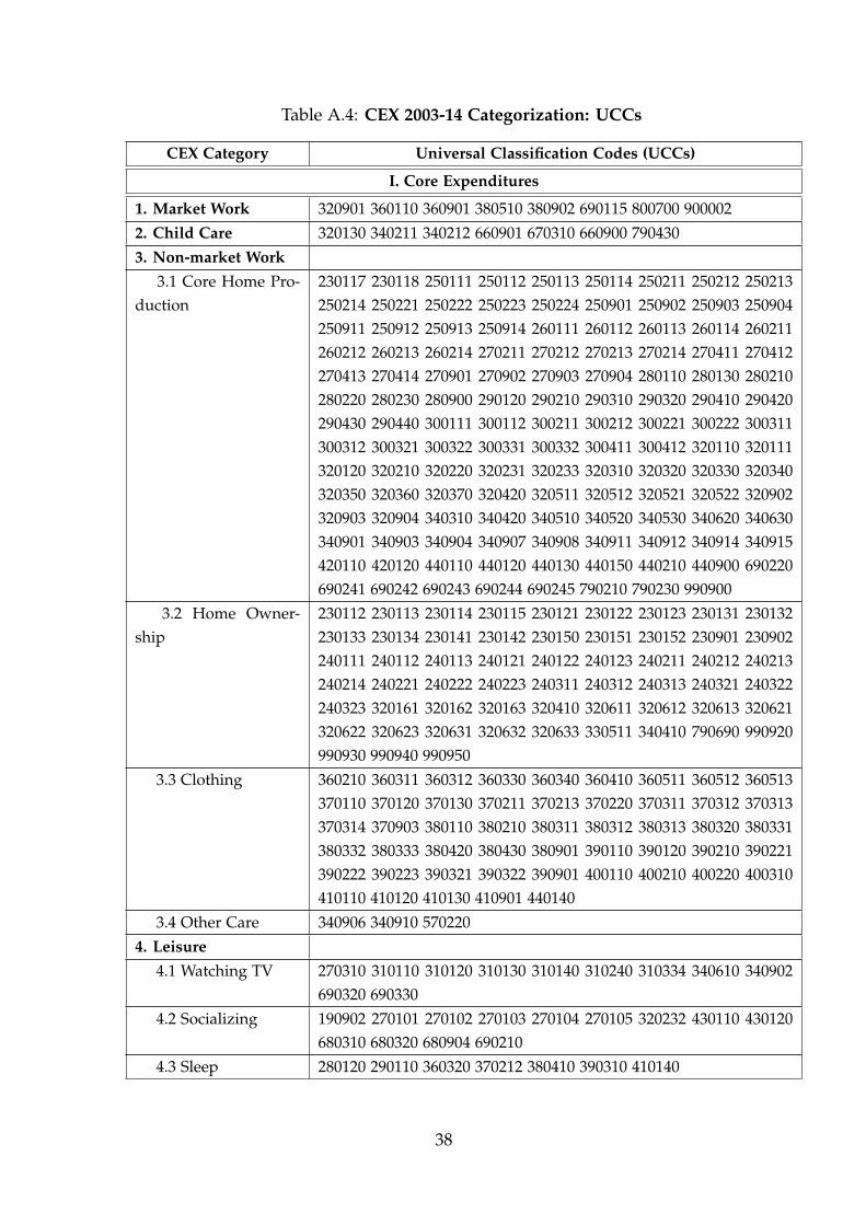
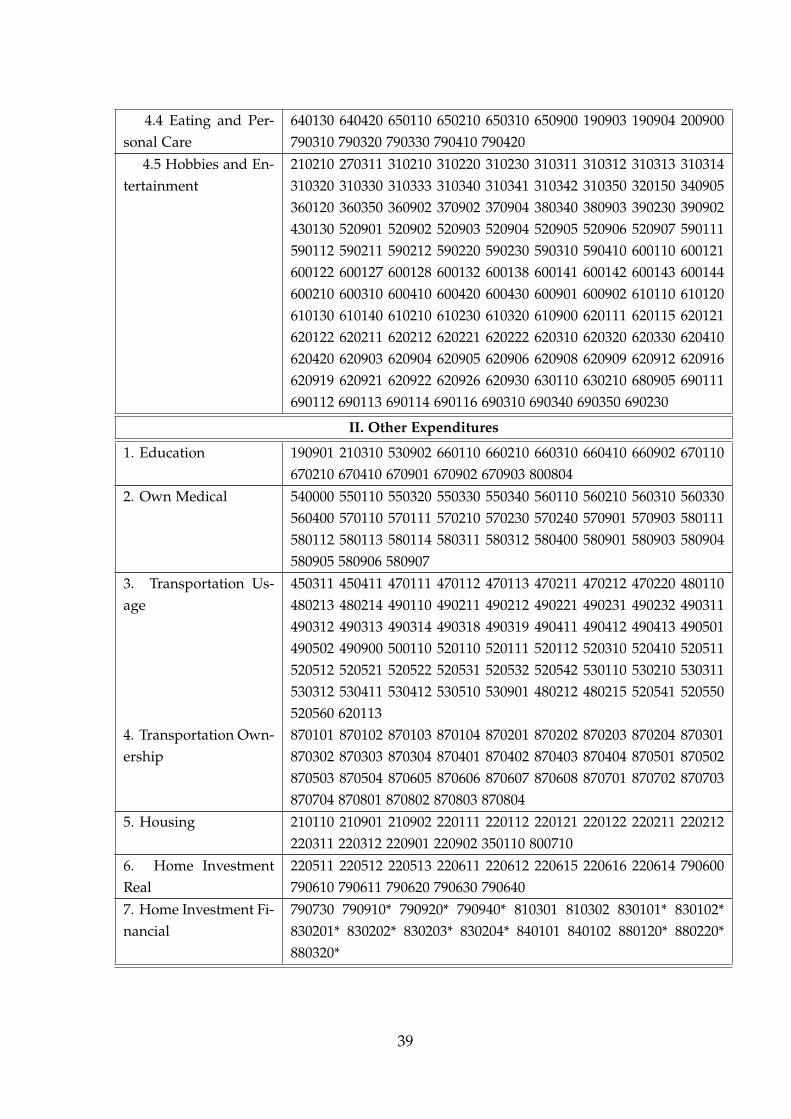
A.3.2. Linking ATUS and CEX
To create consistent expenditure shares and time use associated with each ac-
tivity, we start with the time-use activity categories discussed in section A.1 and
map the associated consumption expenditure categories to the time use categories
as closely as possible. The CEX releases detailed expenditure information in its
MTBI files. Consumption and investment expenditures are organized by Universal
Classification Codes (UCCs). The files contain approximately 600 different UCCs,
with one record for every purchase of the CU in a given month. The Bureau of
34
Labor Statistics (BLS) provides summary level variables that aggregate a certain
set of UCCs. These summary variables serve as a guideline for the classification
of expenditure categories. For every summary variable, we check the underlying
UCCs and, if necessary, refine the categorization. Table A.3 provides a description
of the expenditures associated with each category, while table A.4 documents the
corresponding UCCs.
In additional to consumption expenditures, the CEX also collects information
on the purchases and sales of assets. We classify the purchase and investment of
housing and vehicles as separate categories, as they involve investment decisions
and cannot be linked to a particular activity. Note that the investment categories
only contain outlays related to the acquisition of new assets. Expenditures asso-
ciated with the maintenance or repair of housing or vehicles, that the CU already
owns, are matched with a corresponding time use category.
We exclude investment expenditures in the analysis for two reasons. First,
they can not be linked to a specific time-use category. Second, the static model
employed in this paper can not be used to analyze the investment decisions. Simi-
larly, we exclude education and medical care time and expenditures from our main
analysis as we view them as human capital investments. We exclude time spent on
civic and unclassified activities because they can not be linked to any expenditure
categories. Expenditures spent on transportation usage cannot be separated into
direct transportation costs associated with actual activities. We therefore exclude
it from our analysis as well. We refer to the expenditures included in our analysis
as “core expenditures." Over the sample period, our measure of core expenditures
accounts for slightly over one-half of all consumption expenditures reported in the
CEX.
The ATUS and the CEX cannot be linked at the household level. We therefore
link them either by education or income every year. We partition the observations
into four education groups: less than high school, high school, some college, col-
lege and above. In both the ATUS and the CEX, the highest level of educational
attainment of the reference person determines which education bin the household
is assigned to.
35
To partition data by household income, we first use the continuous informa-
tion on family income before taxes from the CEX to construct weighted income
quartiles in each survey year using survey weights. We drop negative incomes as
well as the bottom and top 5% of the income distribution. We find that the 25th
percentile is $26,600, the 50th percentile is $50,000, the 75th percentile is $83,900.
In the ATUS, combined income of all family members during the last 12 month
is only reported in bins and not as a continuous variable. We thus chose the bins
that most closely approximate the quartiles derived from the CEX. While we can
match the 50th percentile exactly, we have to move the cut off points for the 25th
and 75th percentile, so we can define income groups consistently across both data
sets. The bin that encompasses the 75th percentile in the CEX ranges from $75,000
to $99,999 in the CEX. Thus, we chose $99,999 in both data sets as the cut off point
for the highest income group (group 4). Similarly, we move the cut off for the 25th
percentile to $25,000 and define the lowest income group (group 1) as any family
with income below this threshold.
Table A.3: CEX 2003-14 Categorization
CEX Category Description of Expenditures
I. Core Expenditures
1. Market Work Office furniture for home use; suits and uniforms for men and women;personal digital assistants; meals received as pay; occupational expenses
2. Child Care Infant’s equipment; babysitting and child day care; school books for daycare centers and nursery schools; school meals for preschool and schoolage children
3. Non-market Work3.1 Core Home Pro-
ductionUtilities, fuels and public services (excl. telephone services); house-hold textiles (excl. bedroom linens); furniture (excl. mattresses and newsprings); major appliances; small appliances; non-permanent carpetsquares; blinds; clocks; lamps; decorative items; kitchen utensils; house-hold services; rental of furniture; rental of household and office equip-ment for non-business use; management fees; other apparel products andservices (excl. watches and jewelry, clothing rental); food at home (excl.food or board at school); other household expenses (excl. computers andsoftware for non-business use)
3.2 Home Ownership Maintenance, repairs and other expenses (excl. homeowner’s insurance,parking and management fees); floor coverings (excl. non-permanent car-pet squares); installed and non-installed wall-to-wall carpeting; buildingan attic, a pool or finishing the basement
36
3.3 Clothing Clothing for men and women (excl. suits and uniforms, nightwear, sportscoats, active sportswear, other sportswear and costumes); clothing for boysand girls (excl. nightwear, active sportswear and costumes); clothing forchildren (excl. sleeping garments); footwear; clothing rental
3.4 Other Care Care for invalids or elderly persons; adult care centers; care in nursinghome (net outlay)
4. Leisure4.1 Watching TV Cable services; TVs; video streaming; satellite dishes; repair, rental and
installation of TV and satellite equipment4.2 Socializing Catered affairs; live entertainment; party supplies; telephone services and
devices; watches; jewelry; dating services4.3 Sleep Bedroom linens; mattresses and new springs; nightwear4.4 Eating and Per-
sonal CarePersonal care appliances and services; rental and repair of personal careappliances; food and beverages during out-of-town trips; alcoholic bever-ages; dining out at restaurants
4.5 Hobbies and Enter-tainment
Trip expenditures on lodging; satellite radio services; video, radio andsound equipment; records, CDs, videos and audio tapes; streaming audiofiles; outdoor equipment; sport coats, sportswear and costumes; travelitems; rental or purchase of trailer-type camper, boat or aircraft; reading(excl. encyclopedia); miscellaneous entertainment outlays; pets, toys andplayground equipment; musical instruments; photographic equipment;event fees and admission; computers and software for non-business use;tobacco and smoking supplies
II. Other Expenditures
1. Education Food or board at school; housing at school; private school bus; educationalexpenses such as tuition and school books (excl. books for day care center);encyclopedia; test prep and tutoring services; support for college students
2. Own Medical prescription drugs; health insurance; medical services (excl. care in nurs-ing home); medical supplies
3. Transportation Usage Gasoline and motor oil, maintenance and repairs and vehicle insurancefor any type of vehicle; public transportation; vehicle registration; driver’slicense; vehicle inspection; auto and truck or van rental; lease charges;parking fees; tolls; vehicle equipment and services; GPS; automobile clubmembership
4. Transportation Owner-ship
Outlays for new, used and other vehicle purchases; outlays for motoredand non-motored recreational vehicles
5. Housing Rent of dwelling; ground rent; fire and extended coverage insurance;homeowners’ insurance; property taxes; mortgage interest; parking; rentas pay
6. Home Investment Real Original carpeting; addition, alteration or new construction of dwellings;New dishwasher, garbage disposal or range hood; Management, security,parking; special assessment fees
7. Home Investment Fi-nancial
Closing costs, special mortgage payments; reduction of mortgage princi-pal; reduction of principal on home equity loan; special assessment forroads, streets
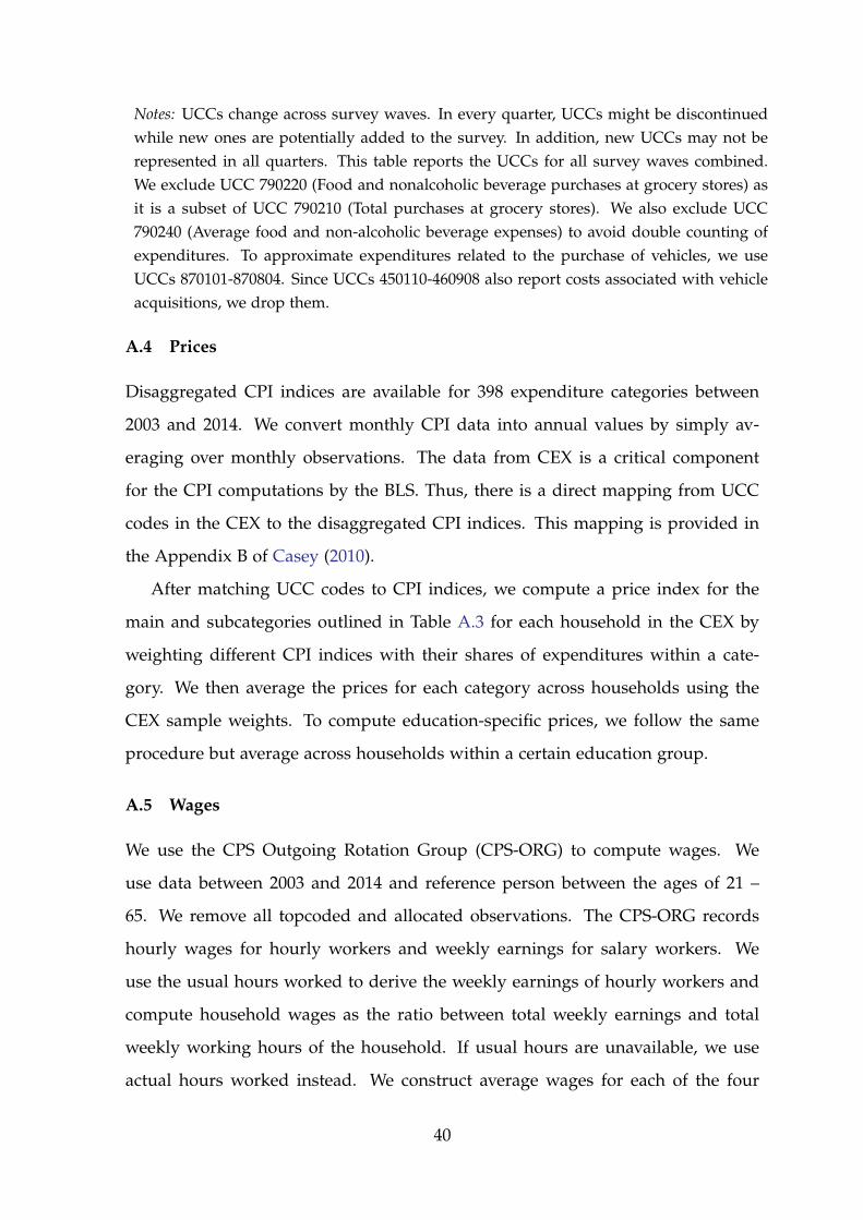
Notes: UCCs change across survey waves. In every quarter, UCCs might be discontinuedwhile new ones are potentially added to the survey. In addition, new UCCs may not berepresented in all quarters. This table reports the UCCs for all survey waves combined.We exclude UCC 790220 (Food and nonalcoholic beverage purchases at grocery stores) asit is a subset of UCC 790210 (Total purchases at grocery stores). We also exclude UCC790240 (Average food and non-alcoholic beverage expenses) to avoid double counting ofexpenditures. To approximate expenditures related to the purchase of vehicles, we useUCCs 870101-870804. Since UCCs 450110-460908 also report costs associated with vehicleacquisitions, we drop them.
A.4 Prices
Disaggregated CPI indices are available for 398 expenditure categories between
2003 and 2014. We convert monthly CPI data into annual values by simply av-
eraging over monthly observations. The data from CEX is a critical component
for the CPI computations by the BLS. Thus, there is a direct mapping from UCC
codes in the CEX to the disaggregated CPI indices. This mapping is provided in
the Appendix B of Casey (2010).
After matching UCC codes to CPI indices, we compute a price index for the
main and subcategories outlined in Table A.3 for each household in the CEX by
weighting different CPI indices with their shares of expenditures within a cate-
gory. We then average the prices for each category across households using the
CEX sample weights. To compute education-specific prices, we follow the same
procedure but average across households within a certain education group.
A.5 Wages
We use the CPS Outgoing Rotation Group (CPS-ORG) to compute wages. We
use data between 2003 and 2014 and reference person between the ages of 21 –
65. We remove all topcoded and allocated observations. The CPS-ORG records
hourly wages for hourly workers and weekly earnings for salary workers. We
use the usual hours worked to derive the weekly earnings of hourly workers and
compute household wages as the ratio between total weekly earnings and total
weekly working hours of the household. If usual hours are unavailable, we use
actual hours worked instead. We construct average wages for each of the four
Notes: Households are grouped into income quartiles. Consumption expenditures areexpressed as a fraction of core expenditures. Time use is reported as weekly hours.
Notes: Households are grouped into income quartiles. Consumption expenditures areexpressed as a fraction of core expenditures. Time use is reported as weekly hours.
42
C Identification of Parameters
Figure C.3: Identification of Parameters
0.124
0.125
0.126
0.127
0.128
1.5 2.0 2.5
ξcc
Sum
of S
quar
es
0.4
0.8
1.2
1.6
0.8 1.0 1.2 1.4
ξnm
Sum
of S
quar
es
0.124
0.126
0.128
1.6 2.0 2.4
ξtv
Sum
of S
quar
es
0.15
0.20
0.25
0.30
1.0 1.2 1.4 1.6
ξsoc
Sum
of S
quar
es
0.15
0.20
0.25
0.30
1.4 1.6 1.8 2.0 2.2 2.4 2.6
ξepcS
um o
f Squ
ares
0.15
0.20
0.25
0.30
1.50 1.75 2.00 2.25 2.50
ξol
Sum
of S
quar
es
page 1 of 1
0.13
0.14
0.15
0.16
0.17
0.05 0.06 0.07 0.08 0.09αcc
Sum
of S
quar
es0
1
2
0.25 0.30 0.35 0.40αnm
Sum
of S
quar
es
0.2
0.3
0.4
0.5
0.6
0.150 0.175 0.200 0.225 0.250αtv
Sum
of S
quar
es
0.15
0.20
0.25
0.08 0.10 0.12 0.14αsoc
Sum
of S
quar
es
0.2
0.3
0.4
0.5
0.12 0.15 0.18 0.21αepc
Sum
of S
quar
es
0.5
1.0
1.0 1.2 1.4 1.6ρ
Sum
of S
quar
es
page 1 of 1
0.124
0.128
0.132
0.136
0.06 0.07 0.08 0.09 0.10κcc
Sum
of S
quar
es
0.25
0.50
0.75
1.00
0.4 0.5 0.6 0.7κnm
Sum
of S
quar
es
0.13
0.14
0.15
0.16
0.17
0.08 0.10 0.12κtv
Sum
of S
quar
es
0.14
0.16
0.18
0.15 0.20 0.25κsoc
Sum
of S
quar
es
0.2
0.3
0.100 0.125 0.150 0.175κepc
Sum
of S
quar
es
0.15
0.20
0.25
0.30
0.125 0.150 0.175 0.200κol
Sum
of S
quar
es
page 1 of 1
Notes: Each sub-plot depicts the value of the objective function when a given parameter valuechanges in a neighborhood of its estimated value.
43
D Robustness: Estimation with Education-Specific Prices
Table D.5: Parameter Estimates
A. Becker Model
Child Non-market TV Social Eat & Pcare Hobbiesξ 2.368 1.086 2.049 1.337 1.986 1.974
Notes: The table reports the means of the bootstrapped distributions for the preferenceparameters of the four models considered. These are described in Sections 3.1, 3.2, 3.3 and3.4, respectively. Bootstrapped standard errors are shown in parentheses.
44
Table D.6: Dispersion in Hours Worked - Data vs. Models
Figure D.4: Response of Hours Worked to a Percentage Wage Change
0 0.2 0.4 0.6 0.8 1% Change in Wages
0
0.05
0.1
0.15
0.2
0.25
0.3
% C
hang
e in
Hou
rs W
orke
d
B: edu1B: edu2B: edu3B: edu4
S: edu1S: edu2S: edu3S: edu4
(a) Becker vs. Standard
0 0.2 0.4 0.6 0.8 1% Change in Wages
0
0.05
0.1
0.15
0.2
0.25
0.3%
Cha
nge
in H
ours
Wor
ked
B: edu1B: edu2B: edu3B: edu4
M: edu1M: edu2M: edu3M: edu4
(b) Becker vs. Multiple–Goods
0 0.2 0.4 0.6 0.8 1% Change in Wages
0
0.05
0.1
0.15
0.2
0.25
0.3
% C
hang
e in
Hou
rs W
orke
d
B: edu1B: edu2B: edu3B: edu4
B2: edu1B2: edu2B2: edu3B2: edu4
(c) Becker vs. Two Activity
Notes: ’B’ refers to the Becker model, ’S’ to the Standard model, ’M’ to the Multiple Goodsmodel, and ’B2’ to the Two Activity model. The four education categories are definedas follows: edu1 - less than high school, edu2 - high school, edu3 - some college, edu4 -college and above.
45
E Model Solution
E.1 Becker Model
Let i be the index for an activity and j be the index for education. For the ease of
notation, define Cj =
(∑i αic
ρ−1ρ
ij
) ρρ−1
. The utility function for education j is then
given by:
U(Cj) = log(Cj), Cj =
(∑
iαic
ρ−1ρ
ij
) ρρ−1
, cij =
(κix
ξi−1ξi
ij + (1− κi)`ξi−1
ξiij
) ξiξi−1
.
The budget constraint is:
∑i
pijxij = wj(1−∑i`ij). (4)
Each education group maximizes utility subject to the budget constraint. Let λj
be the lagrangian multiplier. The F.O.Cs are as follows:
∂U∂cij
∂cij
∂xij= λj pij (5)
∂U∂cij
∂cij
∂`ij= λjwj (6)
Taking the ratio between these two equations gives:
`ij
xij=
(pij
wj
)ξi (1− κi
κi
)ξi
. (7)
Simple manipulations of the definition of cij gives:
cij = xijκ
ξiξi−1
i
(1 +
1− κi
κi(`ij
xij)
ξi−1ξi
) ξiξi−1
. (8)
Plugging equation (7) into the above equation gives:
cij = xijκ
ξiξi−1
i
(1 + (
1− κi
κi)ξi(
pij
wj)ξi−1
) ξiξi−1
(9)
Define Mij = κ
ξiξi−1
i
(1 + (1−κi
κi)ξi(
pijwj)ξi−1
) ξiξi−1 . We have cij = Mijxij.
From equation (5), we can derive the following equation between activity i and
46
activity 1:∂U∂c1j
∂c1j∂x1j
∂U∂cij
∂cij∂xij
=p1j
pij. (10)
Plugging in the partial derivatives gives:
α1c−1ρ
1j (c1jx1j)
1ξ1 κ1
αic−1ρ
ij (cijxij)
1ξi κi
=p1j
pij. (11)
Plugging cij = Mijxij into the above equation gives:
xij
x1j=
(p1j
pij
)ρ (αiκi
α1κ1
)ρ Mρ−ξi
ξiij
Mρ−ξ1
ξ11j
. (12)
Define Ni1j =(
p1jpij
)ρ (αiκiα1κ1
)ρ M
ρ−ξiξi
ij
Mρ−ξ1
ξ11j
. Then, xij = Ni1jx1j. This and equations (7)
give `ij as a function of x1j:
`ij =
(pij
wj
)ξi (1− κi
κi
)ξi
Ni1jx1j. (13)
The budget constraint can be rewritten as follows:
x1j ∑i
pijxij
x1j= wj
(1−∑
i`ij
). (14)
x1j ∑i
pijNi1j = wj
1−∑i
(pij
wj
)ξi (1− κi
κi
)ξi
Ni1jx1j
. (15)
Solve x1j from the above equation gives:
x1j =wj
∑i pijNi1j + wj ∑i
(pijwj
)ξi(
1−κiκi
)ξiNi1j
(16)
xij can then be solved from equation (12) and `ij can be solved from equation (7).
47
E.2 Standard Model
Define Csj =
(φs(xs
j )σs−1
σs + (1− φs)(`sj)
σs−1σs) σs
σs−1 . The utility function for eduction j
is given by:
U(Csj ) = log(Cs
j ), Csj =
(φs(xs
j )σs−1
σs + (1− φs)(`sj)
σs−1σs) σs
σs−1 .
Normalize the price of xsj to one. The budget constraint is
xsj = wj(1− `s
j). (17)
Let λsj be the lagrange multiplier. The first order conditions are:
(Csj )
1σs φs(xs
j )− 1
σs = λsj (18)
(Csj )
1σs (1− φs)(`s
j)− 1
σs = λsj wj. (19)
The ratio between these two equations gives:
`sj
xsj=
(1
wj
)σs (1− φs
φs
)σs
. (20)
Plug equation (20) into the budget constraint gives:
xsj =
wj
1 + (wj)1−σs(
1−φs
φs
)σs . (21)
E.3 Multiple Goods Model
Define Cmj =
(φm(Xm
j )σm−1
σm + (1− φm)(`mj )
σm−1σm) σm
σm−1 . The utility function for edu-
cation j is given by:
U(Cmj ) = log(Cm
j ), Cmj =
(φm(Xm
j )σm−1
σm + (1− φm)(`mj )
σm−1σm) σm
σm−1
Xmj =
(∑
iµi(xm
ij )η−1
η
) ηη−1
48
The budget constraint is:
∑i
pijxmij = wj(1− `m
j ). (22)
Let λmj be the lagrange multiplier. The first order conditions are given by:
∂UCm
j
∂Cmj
∂Xmj
∂Xmj
∂xmij
= λmj pij (23)
∂UCm
j
∂Cmj
∂`mj
= λmj wj. (24)
Using (23) between activity i and activity 1,xm
ijxm
1jcan be derived as follows.
∂Xmj
∂xm1j
∂Xmj
∂xmij
=µ1(xm
1j)− 1
η
µi(xmij )− 1
η
=p1j
pij, (25)
xmij
xm1j
=
(p1j
pij
)η (µi
µ1
)η
. (26)
Plugging (26) into the expression for Xmj gives:
Xmj = µ
ηη−11
∑i
(µi
µ1
)η(
p1j
pij
)η−1
ηη−1
xm1j. (27)
Define Mmj = µ
ηη−11
[∑i
(µiµ1
)η ( p1jpij
)η−1] η
η−1
. Hence Xmj = Mm
j xm1j.
Taking ratio between (23) for activity 1 and (24) gives:
∂Cmj
∂Xmj
∂Xmj
∂xm1j
∂Cmj
∂`mj
=
φm(Xmj )− 1
σm µ1
(Xm
jxm
1j
) 1η
(1− φm)(`mj )− 1
σm=
p1j
wj, (28)
`mj =
(p1j
wj
)σm (1− φm
φmµ1
)σm
(Mmj )
η−σmη xm
1j. (29)
Plugging (26) and (29) into the budget constraint gives: