37
© Oxford University Press, 2009. All rights reserved. Burda & Wyplosz MACROECONOMICS 5 th edn Chapter 13 Aggregate Demand and Aggregate Supply
| Date post: | 07-Feb-2018 |
| Category: |
Documents |
| Upload: | phamnguyet |
| View: | 226 times |
| Download: | 2 times |
© Oxford University Press, 2009. All rights reserved.
Burda & Wyplosz MACROECONOMICS 5th edn
Chapter 13
Aggregate Demand and Aggregate Supply
Burda & Wyplosz MACROECONOMICS 5/e
2
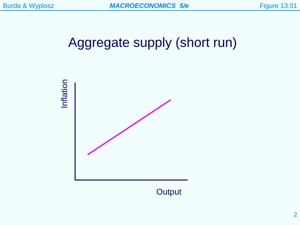
Aggregate supply (short run)
Figure 13.01
Infla
tion
Output
Burda & Wyplosz MACROECONOMICS 5/e
3
Why is the short-run AS curve upward sloping? It is derived by combining a short-run Phillips curve with
Okun’s law. It shows how output varies with inflation for a given
expected rate of inflation. When inflation is higher than expected, real wages fall
below their equilibrium level and hence firms increase output.

Burda & Wyplosz MACROECONOMICS 5/e
4
What shifts the short-run AS curve?
The short-run AS curve shifts for the same reasons as the short-run Phillips curve. An increase in the expected rate of inflation shifts it to the left, as this pushes up the rate of increase of input prices (including wages).
Output
Infla
tion
AS
AS`
Burda & Wyplosz MACROECONOMICS 5/e
5 © Oxford University Press, 2009. All rights reserved.
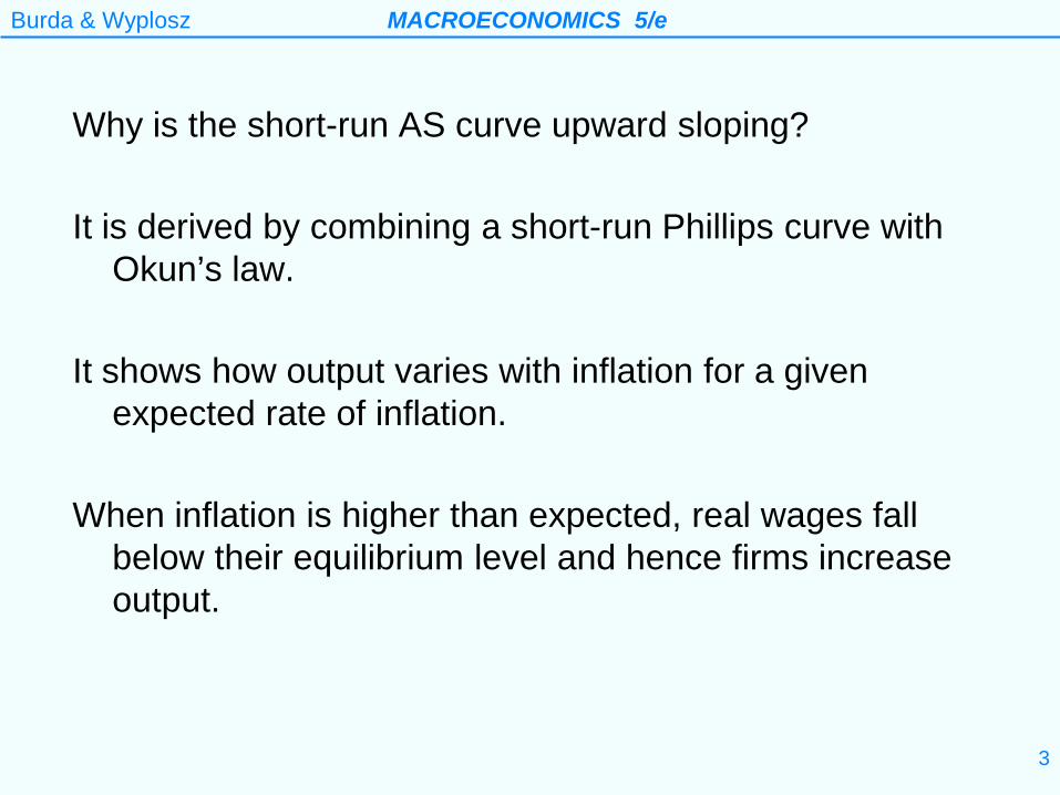
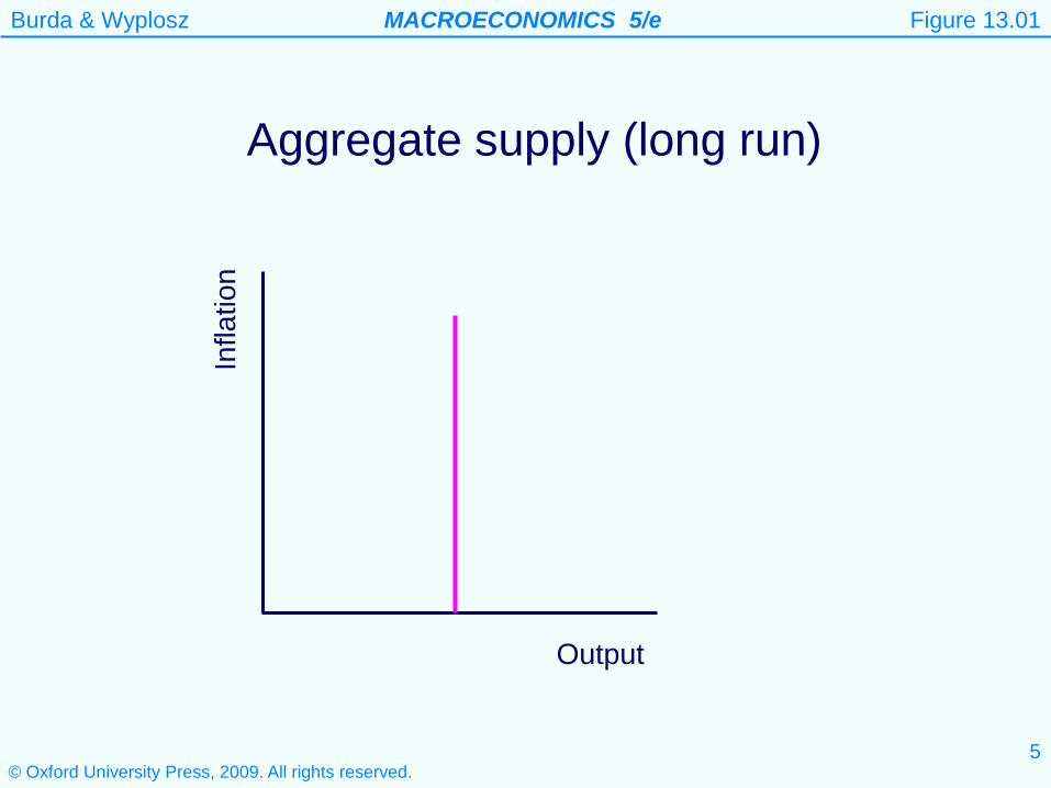
Aggregate supply (long run)
Figure 13.01
Infla
tion
Output
Burda & Wyplosz MACROECONOMICS 5/e
6
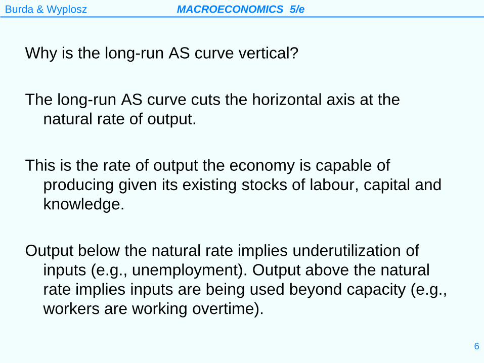
Why is the long-run AS curve vertical? The long-run AS curve cuts the horizontal axis at the
natural rate of output. This is the rate of output the economy is capable of
producing given its existing stocks of labour, capital and knowledge.
Output below the natural rate implies underutilization of
inputs (e.g., unemployment). Output above the natural rate implies inputs are being used beyond capacity (e.g., workers are working overtime).
Burda & Wyplosz MACROECONOMICS 5/e
7 © Oxford University Press, 2009. All rights reserved.
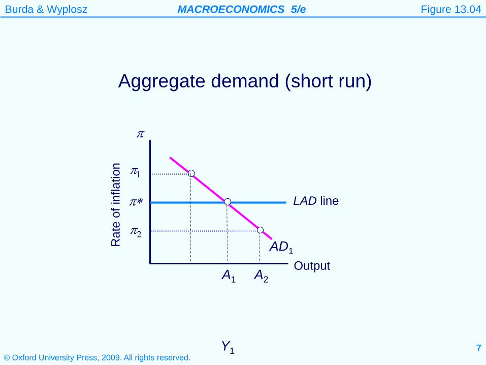
Aggregate demand (short run)
Rat
e of
infla
tion
Output
LAD line
A1 A2
Y1
π
Figure 13.04
AD1
π1
π∗
π2
7
Burda & Wyplosz MACROECONOMICS 5/e
8
Why is the short-run AD curve downward sloping? π* is the rate of inflation in the rest of the world. If π > π*
(holding the exchange rate fixed) then the home country becomes less competitive and exports (X) fall and imports (M) rise. This causes AD to fall.
Note: AD = C + I + G + X - M
Burda & Wyplosz MACROECONOMICS 5/e
9
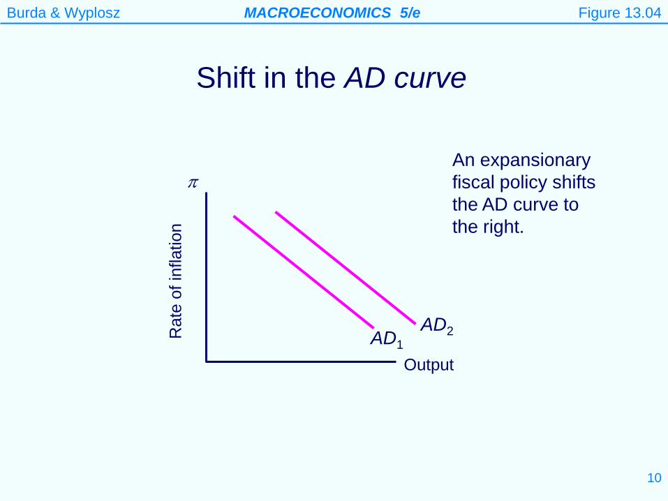
Shifts in the short-run AD curve
The AD curve will shift if aggregate demand changes for some reason other than a change in π.
For example, in the fixed exchange rate case, an increase in government expenditure, a fall in taxes, or a rise in net exports (caused by something other than a change in π), would all shift the AD curve to the right.
Note: Under fixed exchange rates, if π > π*, then over time the AD curve shifts to the left. This is because each period that π > π*, the country becomes less and less competitive, and hence net exports continue to fall.
Burda & Wyplosz MACROECONOMICS 5/e
10
AD2
Shift in the AD curve
Rat
e of
infla
tion
Output
π
An expansionary fiscal policy shifts the AD curve to the right.
Figure 13.04
AD1
Burda & Wyplosz MACROECONOMICS 5/e
11 © Oxford University Press, 2009. All rights reserved.
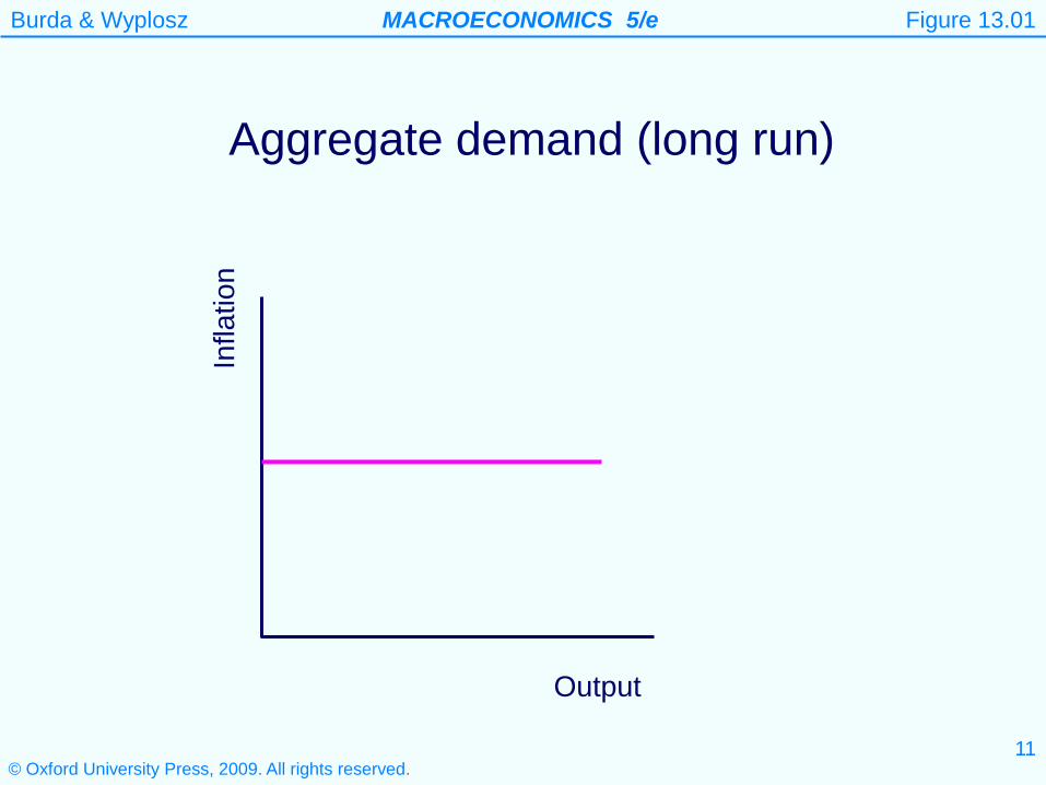
Aggregate demand (long run)
Figure 13.01
Infla
tion
Output
Burda & Wyplosz MACROECONOMICS 5/e
12
Why is the long-run AD (LAD) curve horizontal? In the long-run π = π*. Under fixed exchange rates, π > π*
would imply the home country becoming less and less competitive. Exports fall and imports rise pushing down aggregate demand (and hence π).
The leftward shift in the AD curve continues until once
again π = π*.
Burda & Wyplosz MACROECONOMICS 5/e
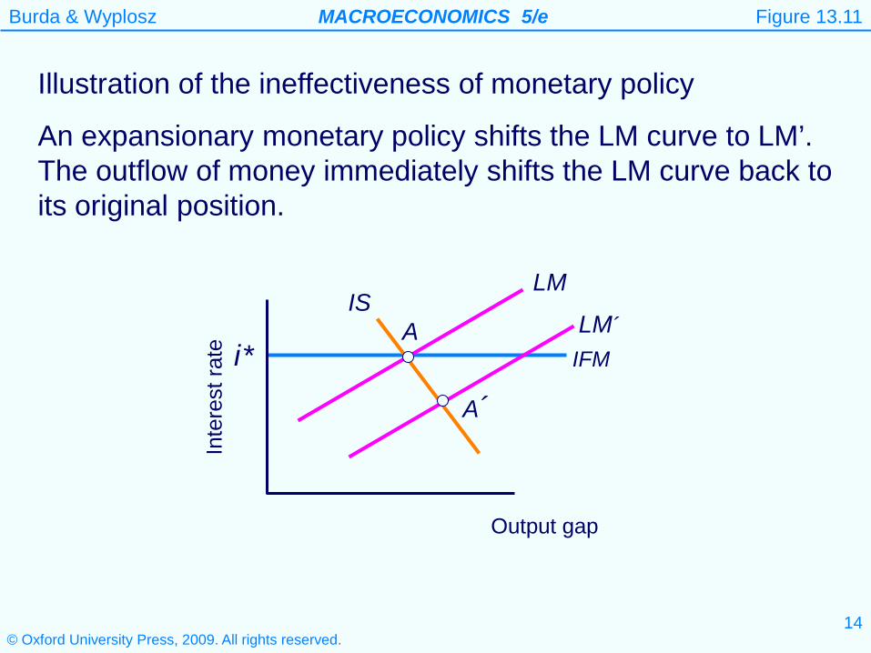
Monetary policy does not work under fixed exchange rates An expansionary monetary policy fails to shift the LM curve since the increased money supply immediately leaves the country (in search of a higher rate of interest). Hence the LM curve does not move and the interest rate remains at i* (the international interest rate). Without a change in i there is no transmission mechanism for monetary policy.
13
Burda & Wyplosz MACROECONOMICS 5/e
14 © Oxford University Press, 2009. All rights reserved.
Illustration of the ineffectiveness of monetary policy
An expansionary monetary policy shifts the LM curve to LM’. The outflow of money immediately shifts the LM curve back to its original position.
Inte
rest
rate
Output gap
LM
A´
A LM´
IFM
IS
Figure 13.11
i*
Burda & Wyplosz MACROECONOMICS 5/e
15
Fiscal policy under fixed exchange rates
Figure 13.06
Burda & Wyplosz MACROECONOMICS 5/e
16
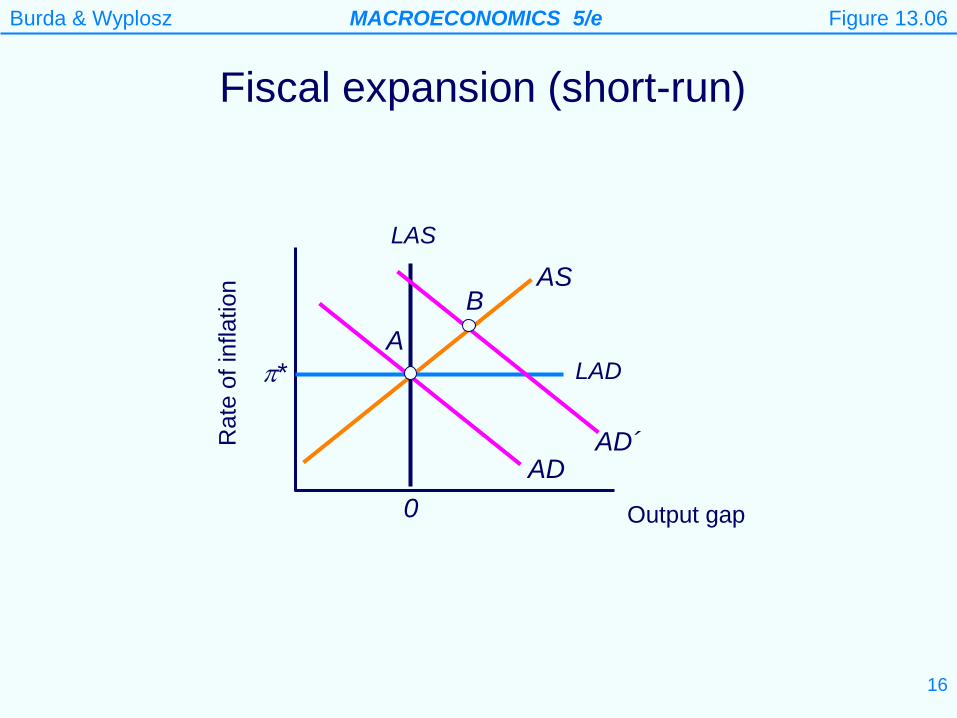
Fiscal expansion (short-run)
Figure 13.06
Rat
e of
infla
tion
Output gap
LAD
0
π*
AS
AD
AD´
A
B
LAS
Burda & Wyplosz MACROECONOMICS 5/e
17
AS´´ AS´
Figure 13.06
Rat
e of
infla
tion
Output gap
LAD
0
π*
AD AD´
A
B D
LAS
C
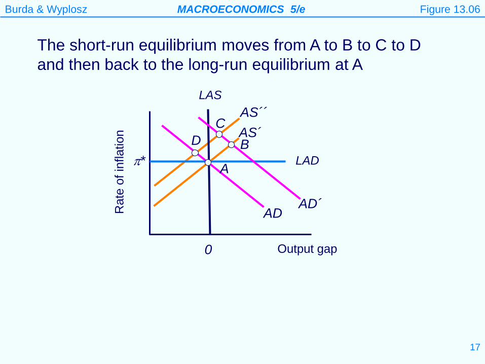
The short-run equilibrium moves from A to B to C to D and then back to the long-run equilibrium at A
Burda & Wyplosz MACROECONOMICS 5/e
18
An expansionary fiscal policy shifts the AD curve to the right. Next the AS curve shifts to the left (since output is above its natural rate). Now the AD curve starts shifting to the left since inflation is higher than in other countries and hence exports are becoming more expensive and imports cheaper. The economy overshoots the LAS curve (i.e., the economy goes into recession). This causes the AS curve to start shifting back to the right. Eventually the economy converges back to its initial starting point.
Burda & Wyplosz MACROECONOMICS 5/e
19
A devaluation
Figure 13.07
Burda & Wyplosz MACROECONOMICS 5/e
20
B
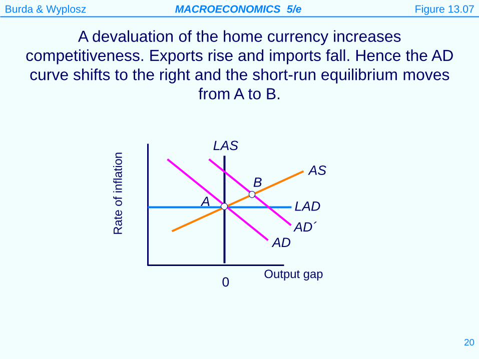
A devaluation of the home currency increases competitiveness. Exports rise and imports fall. Hence the AD curve shifts to the right and the short-run equilibrium moves
from A to B. R
ate
of in
flatio
n
Output gap
LAD A
0
LAS
AS
AD AD´
Figure 13.07
Burda & Wyplosz MACROECONOMICS 5/e
21
The higher rate of inflation in the home country now gradually reduces competitiveness. The economy now follows the same path as after an expansionary fiscal policy. Both the AS and AD curves shift to the left and the economy ends up back at its long-run equilibrium at point A. In other words, the higher domestic inflation rate eventually completely undoes the competitive advantage of the devaluation.
Burda & Wyplosz MACROECONOMICS 5/e
22
0
1
2
3
1994 1996 1998 2000 2002 2004 2006
Denmark
Euro area
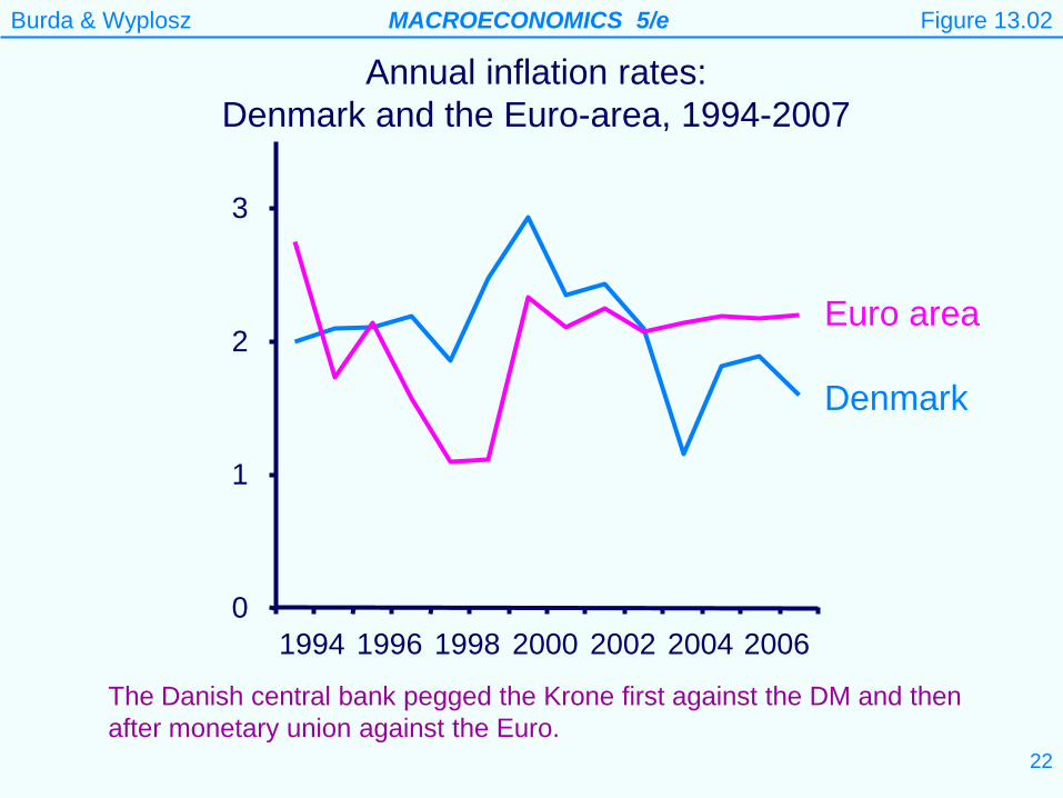
Annual inflation rates: Denmark and the Euro-area, 1994-2007
Figure 13.02
The Danish central bank pegged the Krone first against the DM and then after monetary union against the Euro.
Burda & Wyplosz MACROECONOMICS 5/e
23
Flexible exchange rates:
Under flexible exchange rates the interest rate is endogenous. The central bank can choose its level. A rise in the interest rate reduces investment and appreciates the currency (reducing net exports). These effects combine to shift the AD curve to the left. In other words, the central bank can move the AD curve.
Burda & Wyplosz MACROECONOMICS 5/e
24
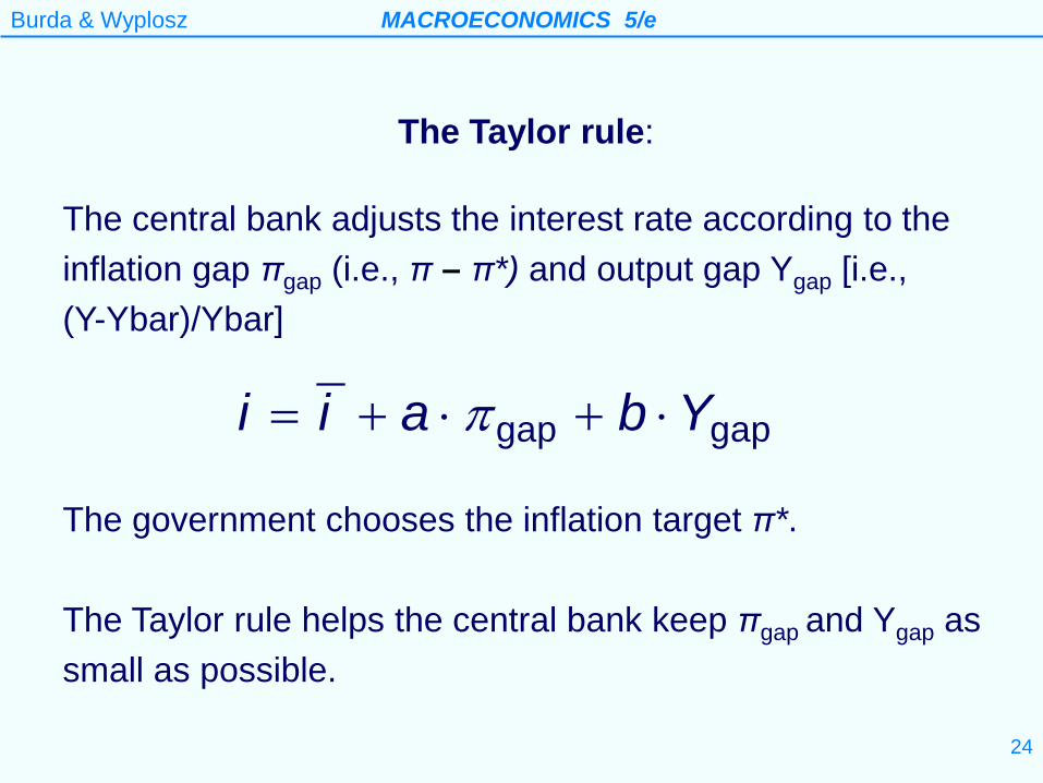
gap gapi i a b Yπ= + ⋅ + ⋅
The Taylor rule:
The central bank adjusts the interest rate according to the inflation gap πgap (i.e., π – π*) and output gap Ygap [i.e., (Y-Ybar)/Ybar]
The government chooses the inflation target π*. The Taylor rule helps the central bank keep πgap and Ygap as small as possible.
Burda & Wyplosz MACROECONOMICS 5/e
25
LAD
AS´ LAS
AS
AD
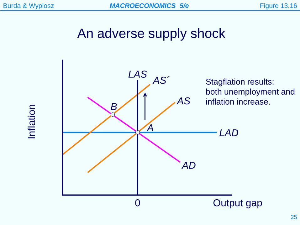
An adverse supply shock In
flatio
n
0
B
Stagflation results: both unemployment and inflation increase.
Figure 13.16
Output gap
A
Burda & Wyplosz MACROECONOMICS 5/e
26
At point B, we have that πgap > 0 and Ygap< 0. So it is not clear from the Taylor rule whether the central bank will raise or lower interest rates. The negative output gap causes wages to start rising at a slower rate. If the central bank does not intervene, the AS curve gradually shifts back to the right. The economy eventually returns to point A.
Burda & Wyplosz MACROECONOMICS 5/e
27
AD´
LAS
AD
AS
An adverse demand shock In
flatio
n
0
A
B
Output gap
LAD
Burda & Wyplosz MACROECONOMICS 5/e
28
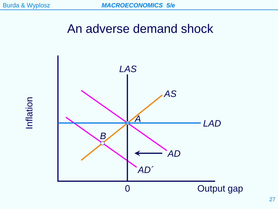
Now at point B, we have that πgap < 0 and Ygap< 0. So from the Taylor rule it is clear that the central bank will lower interest rates. This shifts the AD curve to the right and returns the economy to point A.
Burda & Wyplosz MACROECONOMICS 5/e
29
Monetary policy under flexible exchange rates
A distinction can be drawn between
(i)changes in interest rates following directly from the Taylor rule
(ii)changes in the Taylor rule (such as a reduction in the inflation target).
When the textbook talks about a change in monetary policy it means (ii).
This is confusing since in other contexts one may want to say that a change in monetary policy occurs whenever the central bank changes short term interest rates.
Burda & Wyplosz MACROECONOMICS 5/e
30
AD´
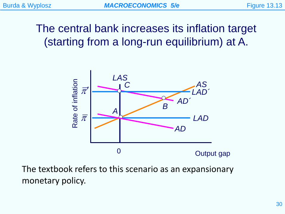
The central bank increases its inflation target (starting from a long-run equilibrium) at A.
Figure 13.13
Rat
e of
infla
tion
Output gap 0
AS LAS
π LAD A
C π ′ LAD´
B
AD
The textbook refers to this scenario as an expansionary monetary policy.
Burda & Wyplosz MACROECONOMICS 5/e
31
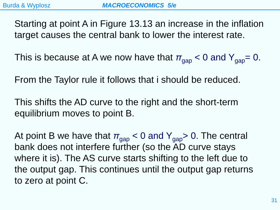
Starting at point A in Figure 13.13 an increase in the inflation target causes the central bank to lower the interest rate. This is because at A we now have that πgap < 0 and Ygap= 0. From the Taylor rule it follows that i should be reduced. This shifts the AD curve to the right and the short-term equilibrium moves to point B. At point B we have that πgap < 0 and Ygap> 0. The central bank does not interfere further (so the AD curve stays where it is). The AS curve starts shifting to the left due to the output gap. This continues until the output gap returns to zero at point C.
Burda & Wyplosz MACROECONOMICS 5/e
32
LAD
AS´ LAS
AS
AD
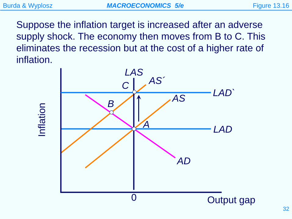
Suppose the inflation target is increased after an adverse supply shock. The economy then moves from B to C. This eliminates the recession but at the cost of a higher rate of inflation.
Infla
tion
0
B
Figure 13.16
Output gap
A
LAD` C
Burda & Wyplosz MACROECONOMICS 5/e
33
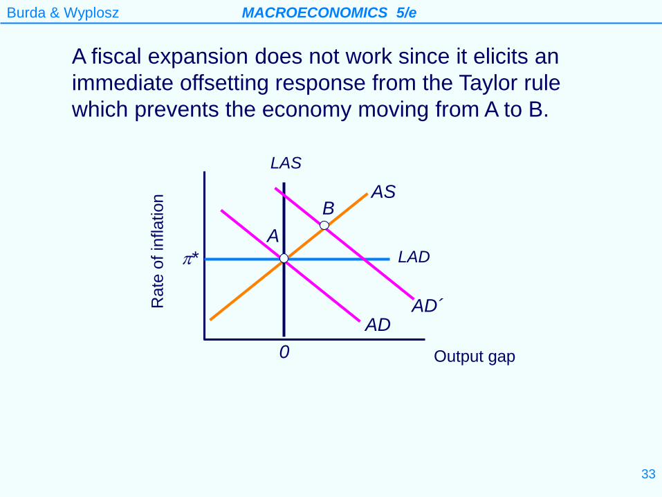
A fiscal expansion does not work since it elicits an immediate offsetting response from the Taylor rule which prevents the economy moving from A to B.
Rat
e of
infla
tion
Output gap
LAD
0
π*
AS
AD
AD´
A
B
LAS
Burda & Wyplosz MACROECONOMICS 5/e
34
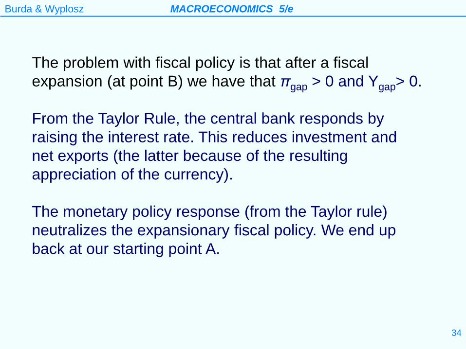
The problem with fiscal policy is that after a fiscal expansion (at point B) we have that πgap > 0 and Ygap> 0. From the Taylor Rule, the central bank responds by raising the interest rate. This reduces investment and net exports (the latter because of the resulting appreciation of the currency). The monetary policy response (from the Taylor rule) neutralizes the expansionary fiscal policy. We end up back at our starting point A.
Burda & Wyplosz MACROECONOMICS 5/e
35
Disinflation Contractionary Monetary Policy
Figure 13.19
Burda & Wyplosz MACROECONOMICS 5/e
36
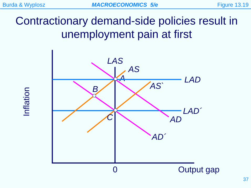
Suppose now the central bank lowers its inflation target. This situation is shown in Figure 13.19. Once the inflation target is lowered we now have that πgap > 0 and Ygap= 0. The Taylor rule now implies that the central bank will raise the interest rate. This shifts the AD curve to the left. The short-run equilibrium moves from A to B (causing a recession). Now the expected rate of inflation falls (since at B the Ygap< 0). The AS curve shifts to the right until the new equilibrium is reached at C.
Burda & Wyplosz MACROECONOMICS 5/e
37
LAD´
AD´
LAS AS
AD
Contractionary demand-side policies result in unemployment pain at first
Infla
tion
0
A B
Figure 13.19
Output gap
LAD
C
AS`


