Business Age, another Source of Employment Growth 1 * Corresponding author. 1 We thank Maryland Department of Labor, Licensing and Regulation (DLLR), Office of Workforce Information and Performance staff for their patient explanation of data field definitions and appropriate data processing steps for our analysis. Ting Zhang*, PhD Research Assistant Professor Jacob France Institute Merrick School of Business University of Baltimore Email: [email protected]Phone: 410-837-6551 David Stevens, PhD Research Professor Jacob France Institute Merrick School of Business University of Baltimore 1420 N. Charles Street Baltimore, Maryland 21201-5779
Transcript
Business Age, another Source of Employment Growth1
* Corresponding author. 1 We thank Maryland Department of Labor, Licensing and Regulation (DLLR), Office of Workforce Informat ion and Performance staff for their patient explanation of data field definitions and appropriate data processing steps for our analysis.
Business Age, another Source of Employment Growth2
ABSTRACT This paper contributes new evidence using recent administrative data to advance what is known about an important, but still controversial, topic among economists—the expected contributions of old and new businesses to employment growth. Improved understanding of the relative place-specific contributions of old and new businesses to employment growth is needed to help policy makers make efficient and effective decisions to hasten and sustain recovery from the current recession. While not an either-or decision, federal, state and local governments are encouraged by competing advocacy groups to favor new incentives for hiring by existing businesses, or to prefer offering of incentives for new business start-ups. Successful employment growth policies will remain complex, place specific and contentious, but new recent information about the origins of employment growth can add a common starting point for consideration of available policy options. Our analysis uses Quarterly Census of Employment and Wages (QCEW) data at the county level for one state, covering business employment dynamics between January 2004 and September 2008.
New transformations of business establishment start and end dates and employment size-class designations are introduced. Innovative transformations of published local unemployment rates incorporate both magnitude and propensity. Based on estimates from multistage econometric modeling with inverse use of instrument variable technique and hierarchical panel data with autocorrelation correction, policy relevant findings include a positive employment growth advantage for older business establishments in more than half of local industry sectors. Established large businesses are typically found in a different spatial pattern and lower count than the distribution of smaller, often newer establishments. This means that the former locales are more dependent upon the success of fewer businesses, including merger and acquisition transactions.
Local unemployment rates impact employment growth. However, it is the unemployment rate trend that consistently associates with employment growth, not the magnitude of the rate per se. Local demographics matter too, for both labor supply and consumer behavior reasons. The local level administrative data source, the unique transformations and measurement, and the model specifications and statistical results presented in this paper offer a new guide for future researchers and policy decision-makers. Local emergence from the U.S. recession that began in December 2007 will be uneven in timing, magnitude and composition. The design and implementation of successful interventions to accelerate and advance local employment growth will depend in part on an improved understanding of the current local economic composition.
2 We thank Maryland Department of Labor, Licensing and Regulation (DLLR), Office of Workforce Informat ion and Performance staff for their patient explanation of data field definitions and appropriate data processing steps for our analysis.
1
I. Introduction Recovery from a recession requires employment growth. With large and growing
national, state and local fiscal challenges it is critical to create jobs smartly and effectively. When many businesses face enormous challenges of their own, what types of business should be targeted by governments for assistance?
For many, pursuit of the ―American Dream‖ involves entrepreneurship and small businesses. The importance of small business has been emphasized for years as a major engine of economic growth and job creation. Entrepreneurship is believed by most observers to have been a major source of America‘s competitive edge in the world economy.
However, small businesses also lose many jobs. Compared with many larger and more mature businesses, small businesses often contribute to limited net job growth. Considering the high failure rate among small businesses, focusing limited financial resources on smaller businesses could be a poor use of resources.
To effectively utilize public resources and efficiently create more jobs, should tax payers‘ money be invested in older or newer businesses, in larger or smaller businesses, and in what type of industries? The ultimate judgment call depends on what type of businesses generates more jobs.
There has been no consensus in previous literature about whether larg or small businesses generate more employment growth. The complexity of business size measurement has contributed to the absence of a consensus. Employment size-class assignment changes as a business grows. Facing competition, ‗grow or out‘ is often the survival rule. This makes the timing of business size measurement crucial. Using base-time-period size to define business size employment gain must always be from smaller employment size classes to larger ones, while employment losses can only arise from larger business being reassigned to smaller employment size classes. Static plant level business employment size class measurement introduces bias.
Unlike business size, business age does not directly define employment growth at the establishment level, though large businesses tend to have been active for a longer time. Our analysis has been motivated by a belief that the impact of business age, in addition to employment size, will provide new policy relevant insights about promising sources of job creation potential. Business age has been somewhat neglected in previous literature, as a factor in employment growth policy.
This paper measures business establishment age and size dynamics by location and tests whether newer or older establishments tend to generate higher net employment growth. Our analysis uses a reliable administrative dataset, the Quarterly Census of Employment and Wages (QCEW). The analysis proceeds in the context of local economic conditions, industry mix and demographic characteristics. A simple economic accounting model using multistage regression estimation with inverse use of instrument variable technique and hierarchical panel data modeling with lagged time effect correction captures interrelationships among the different layers of data and models variable interdependence. To more accurately estimate the impact of local economic setting an innovative transformation of local unemployment rates is introduced.
We begin with a review of pertinent literature in Section II. Section III introduces our research hypotheses. Section IV explains the paper‘s methodology. Section V presents results. We conclude with future research directions and policy implications.
2
II. Literature Review
The role of business size on an economy‘s economic growth trajectory and speed has been discussed for many years.. Much of this literature responds to and tests the validity of what is known as ―Gibrat‘s Law‖ (Gibrat, 1931). ―Gibrat‘s Law‖ was a behavioral conjecture proposed to explain the observed business size distribution and speculated that business growth rates are independent of size. While many predecessors have focused on the contribution of smaller and younger businesses to employment growth, there have been counterarguments. Based on various datasets and analytical approaches from different countries the business size effect remains unclear and mixed.
II.1 The Power of the Small and Young
Many studies have found that smaller and younger businesses tend to perform better.
Hansen (1992) used a data set on innovation output to assess the degree to which the level of innovation in manufacturing businesses is influenced by business size and business age. He found that both business size and business age tend to be inversely related to innovative output. He also indicated that it was possible to separate the effects of age and size in assessing the level of innovation. Dunne and Hughes (1994) examined growth and survival amongst quoted and unquoted UK companies in the period 1975-85 and compares the results with earlier UK and US studies. With careful attention paid to problems of sample selection bias, their study found that smaller companies grew faster than larger companies, that Gibrat's Law d id not hold amongst smaller businesses, that age was negatively related to growth, and that these results were not an artifact of sample selection bias. Hart (2000) conducted empirical research on the growth of U.K. companies and found that smaller and younger businesses have been growing more quickly than larger and older businesses and thus generating proportionately more new jobs. Calvo (2006) drew upon a sample of 1272 manufacturing businesses in which only 967 of the businesses survived for the entire ten year period and tested the Gibrat‘s law. The results did not support the various theories of static and dynamic economies of scale that is consistent with main economic theories and empirical results on businesses' growth in the United States. The findings of all the above studies rejected Gibrat‘s law and supported the proposition that small businesses grew faster. Most of the studies use data from manufacturing businesses and many of them are addressing the business size impact in an economy that is not the most recent.
II.2 Other Arguments
Small businesses are not always believed to be so powerful. Davis, et al (1996) used a
plant- level data source, the Longitudinal Research Data (LRD) constructed by the U.S. Census Bureau, for a study of the U.S. manufacturing sector from 1972 to 1988. Their findings suggest that the belief that small businesses are the major contributor of new jobs is largely based on methodological flaws. In particular, their reasoning about the "regression fallacy", i.e., those temporary fluctuations in size systematically biased estimates in favor of small business job creation.
Two issues are related in this "regression fallacy". First is the type of size measure. Many studies use size-classes, instead of continuous size measure. This could overstate the change around the size-class defining threshold values. The second is the timing of size measures. Many
3
studies use base-time-period size measure. When a business experiences positive employment growth and crosses the size boundary, the increase is ascribed to its base-time-period category (i.e., smaller businesses); when the same firm shrinks back its base-year category, all of the job losses are ascribed to larger businesses.
Davis, et al (1996) also indicated that small businesses did not have higher net job creation rates. This research has caught on interests among researchers and concerns among policy makers. Considering the high failure rate of small businesses, Wren and Colin (1998) even believe that, ―wisdom has it that direct financial assistance to small businesses for employment creation may be poor use of resources.‖ However, this ―regression fallacy‖ effect was also argued to be very small and that correcting for it did not lead to qualitative change of the results (Davidsson, Lindmark, and Olofsson, 1998). The Davis, et al (1996) research also only analyzed manufacturing businesses.
In contrast to the existing studies on the relationship between business growth and size (as well as) age, which typically focus on relatively mature industries in developed economies, Das (1995) analyzed business growth patterns for an infant industry in a developing economy. It was found that (a) age positively impacted growth, which is opposite to the result in many previous studies; (b) as in many previous studies, current size negatively impacted growth but the magnitude is much higher; and (c) lagged size negatively impacted growth suggesting that fixed factors became a hindrance to growth in rapidly growing infant industries. This study touched the timing issue of the size measure, which would give business age rather than business size a potential advantage to be used as an indicator for employment growth.
As Haltiwanger and Krizan (1999) indicated, the more important factor to employment growth seemed to be business age, not size. They used the updated LRD U.S. manufacturing data from 1970s to early 1990s. Although this study showed that young businesses exhibited high average net employment growth rates, relative to mature businesses, among mature business (not for the young businesses), net employment growth rates increased with business size. This study also called for attention to idiosyncratic factors. Again this research only addressed manufacturing businesses and employment.
Kaplan (2003) used the annual first job- and worker-flows data set of Mexico during 1994-2000 and found that net job growth rates were higher in older businesses; during the economic crisis of 1995 large businesses outperformed small businesses.
The results based on Persson (2004) study that used data from Sweden in 1987 and 1988, with the exception of the construction industry show that new businesses faced a high risk of closing down and the probability of business survival increased with the age and size of the business. This study also found that the initial business size had a negative effect on employment growth.
II.3 The Impact of Unemployment
While the roles of business size and age in generating employment growth have been
discussed, estimation of economic cycle effects, represented by the unemployment rate, often play a deterministic role. Davis et al. (1996) indicated that job reallocation appears to be driven primarily by idiosyncratic shocks based on the LRD US manufacturing data from 1970s to late 1980s. Stiglbauer, et al (2003) found that job creation increased significantly during cyclical upswings whereas job destruction rose in downturns, using a large Austrian administrative
4
dataset in the period of 1978 to 1998 where ―spurious‖ entries and exits of businesses were corrected for.
The relationship between unemployment and employment growth can also be interpreted through entrepreneurship. Previous literature has identified considerable ambiguities about the relationship between unemployment and entrepreneurship (Audretsch, et al., 2000). Unemployment on the one hand stimulates entrepreneurial activity, which was termed as a ―refugee effect‖ or ―push effect‖; on the other hand, as identified by a very different strand in the literature, higher levels of entrepreneurship reduce unemployment, which was termed as a ―Schumpeter effect‖ or ―pull effect‖.
II.4 Industry Sector & Demographic Characteristic Effects
Other factors that have been identified in the literature to impact employment growth
include industry sectors and demographic characteristics. As indicated, there appear to be substantial differences between industry sectors, as competitive advantage in some was achieved through aggregation (upsizing) and in others through disaggregation (downsizing) of the productive process (Reynolds, 1997). Demographic factors were also found important in explaining firm survival and growth (Persson 2004). III. Hypotheses
The still unclear contribution of business size to employment growth has been attributed
in part to measurement related ―regression fallacy‖. Other contributing factors, such as unemployment rate, industry sectors, and demographic factors and business age could contribute to the controversy as well. Business age has not received as much attention as business size. This might be partially related to the data availability. The accuracy and policy value of business size and age contributions to employment growth depends on how the respective measurements are conducted.
As addressed earlier, the timing of business size and age measurement is important. Previous studies have used a static base time period measure, a lagged time period measure, or a combination of lagged and current time period measure. We use a dynamic longitudinal measure specific to each month when the employment was reported. This measurement is also on a continuous scale1, instead of within size or age classes.
Similarly important is where business size and age are measured. We use location-specific measures to avoid the transitory size fluctuations, to include employment growth due to establishment births and deaths, and to capture net employment growth instead of only gross employment growth.
So, this paper integrates QCEW administrative records with other economic data sets to generate dynamic measures of business age and size at the county level and conducts a longitudinal analysis. The QCEW data set also allows multiple levels of industry sector definition and analysis.
1 Only in the descriptive statistics for the figures, size and age classes are used. In the regressions, continuous size and age measurements are e used.
5
We test the following hypotheses:
Average business age specific to each month has a significant impact on local employment growth, but this establishment age impact differs among industry sectors;
Local unemployment rate dynamics also matter. IV. Methodology
This section introduces our model, data and variable definitions. The analysis is
conducted in the context of industry sectors, using both two-digit and three-digit North American Industry Classification System (NAICS) codes. The geographic unit of analysis adopted is county, and the temporal unit of the analysis is month2. This generates four layers of data—month, county, NAICS two-digit industry code, and NAICS three-digit industry sector code.
We use hierarchical panel data modeling to both interpret the relationship between the key variables and capture the interrelationship between the three cross-sectional layers of the data. For such a panel data, we consider the panel specific serial autocorrelation to capture the time effect. A series of correlograms are conducted to detect the serial autocorrelation. When serial autocorrelations are detected, appropriate time effect vectors are adopted in the models.
The models used in this study also adopt a multi-stage regression approach, based on a simple economic accounting model. The multi-stage regression approach accommodates the nested relationship between the key variables and therefore instrumental variables are used. This specific nested relationship will be further explained in this methodological section.
IV.1 The Data
Availability of the Quarterly Census of Employment and Wages (QCEW) administrative records for authorized use honoring the confidentiality requirements imposed made this study possible. The Bureau of Labor Statistics QCEW program releases quarterly employment and payroll figures based on employer reports covering 98 percent of U.S. jobs. The BLS data releases are available at the county, MSA, state and national levels by industry. Published quarterly, with approximately a six-month lag after the end of each reference quarter, the QCEW combination of frequency, timeliness and detail is unmatched.
Based on an Interagency Agreement between the Maryland Department of Labor Licensing and Regulation, Office of Workforce Information and Performance, and [affiliation omitted during review to ensure anonymity of authors], we received authorized access to Maryland QCEW cross-sectional micro data quarterly from 2004 through, at this writing, third quarter of 2008. Approval for use of the QCEW data is specific to each proposed study design, and preliminary results are subject to the state agency‘s review prior to public release.
The QCEW data file provided us with a recent longitudinal administrative dataset and an opportunity to measure business establishment age specific to each month, including coverage of the 47 months leading up to the beginning of the current recession and the first 10 months of the recession.
The QCEW data features comprehensive coverage of businesses subject to the state‘s unemployment insurance law and reporting requirements. Self-employed individuals and 2 Although QCEW data is a quarterly dataset, the employment information is offered monthly.
6
independent contractors are not included3. The QCEW data has limitations for economic analysis use. For example, accurate reporting of information for multi-establishment corporations across various geographic locations is an unresolved challenge, but there are recent and continuing improvements. We therefore use establishment level data only.
Other data used in this study include Bureau of Labor Statistics local unemployment rate estimates and demographic data from the U.S. Census Bureau. The Census Bureau population data are defined by residence, while the unemployment rate and QCEW data are defined by work location. When we interpret our results, it is therefore necessary to note this difference in data reporting calibration, particularly when employment impacts of population attributes are considered.
IV.2 Variable Measurement
Before explaining our model we turn first to explain measurement caveats for major variables. As mentioned earlier, we focus on establishment level data instead of firm level. In a relatively high resolution research in terms of geography, i.e. at the county level in this study, focusing on establishments rather than firms is more accurate because establishments are more sensitive to local economic conditions. Three types of variables are used. The first type is macroeconomic variables—total employment and unemployment rate estimates. The key dependent variable, monthly total employment (E), is the total count of employment of a county in a reference month. When applied in a panel data regression model, this variable actually measures the net employment growth.
We use an innovative way to transform Bureau of Labor Statistics unemployment rate estimates. Previous literature has identified an uncertain relationship between unemployment rates and entrepreneurial actions. To further clarify the role of unemployment rates, we use two vectors to capture the change of unemployment rates. The level of unemployment rate (U) captures the magnitude of unemployment rate changes; the differenced unemployment rate (dU) captures the direction and trend of unemployment rate changes, whether it is going upward or going downward. At the same magnitude, U, there could be two totally opposite economic situations: one is when the unemployment rate is rising (i.e. a slowing-down economy) and the other is when the unemployment rate is decreasing (i.e. the recovering or growing economy). This differenced term of unemployment rate (dU) in regression reflects the derivative measure of unemployment rates. These two vectors capture additional nuances that the traditional unemployment rate magnitude measure alone does not achieve. Endogeneity is addressed by including three-month lagged values.
The second type of variable used in this study is the establishment level variables—establishment size, establishment count, and establishment age. The establishment size (S) is the average number of employment of an establishment at a reference month in a county. The average is the unweighted arithmetic mean. As addressed earlier, this study measures establishment sizes specific and current to each month and also measures at the county versus plant level, which avoids the timing issue that caused fallacy in previous literature. Each establishment has many values for its size measure along the timeline, if its size changes over time; each county has an average establishment size measure at a specific month.
3 Self-employment is not the focus of our analysis. We are more concerned with the job creation impact of business establishments.
7
Establishment count (C) is the total number of establishments of a county in a reference month. Again, due to the longitudinal nature of the QCEW, we are able to measure the establishment counts of a county specific and current to each month.
Establishment age (A) refers to the average time duration (in months) of a county‘s establishments since their initial liability starting dates. The QCEW data offers information on the specific initial liability date of an establishment. However, some establishments have more than one initial liability dates due to situations like reactivation or just seasonal reopening. To simplify the study, we used the earliest initial liability date of an establishment. Again, the longitudinal nature of the QCEW data enables us to measure the establishment age of a county specific and current to each reference month.
The third type of variables is population attribute variables4: population count, population racial diversity index, population age, and gender ratio. These are control variables. Population count (P) measures the total number of people in a county of a reference year. The population age (PA) measures the arithmetic mean age of a county‘s population in a reference year. The gender ratio (PG) is the ratio of the number of male persons divided by the number of female persons. For the racial diversity index (PR).
We use Simpson's Index of Diversity (Gibbs and Martin, 1962) to compose our racial
diversity index (PR) , where n represents the total number of persons of a particular race and N indicates the total number of persons of all races5.
There is also a time effect. We use the time effect to capture the serial autocorrelation. It could be a variety form of autocorrelation—autoregressive, moving average, or even differencing, depending on the serial autocorrelation detection diagnostics mentioned earlier.
To ensure all the variables are measured at a standardized level, we use the log form for some variables. The models of this study mainly follow the log- linear format. This offers the advantage of identify elasticity between the dependent variables and explanatory variables. However, not all variables are transformed into a log format. For variables that are measured as proportions or falling between 0 and 1, the original values of the variables are retained. For those variables that are at a much larger value scales, a logarithm form is applied to standardize the coefficients. Appendix A summarizes the statistical characteristics of the variables. IV.3 The Model
The basic model of this study starts with a basic employment accounting equation: the total employment of a county (E)6 is a multiplicative result of the average employment per establishment, i.e., establishment size (S) and the total number of establishments in the county, i.e., the count of establishments (C).
E = S * C (1) 4 The population attribute data are annual. The Census Bureau publishes population estimates annually. Timing of the population data estimate is not consistent with QCEW data collection, nor are the estimat ion methods. Those differences in data calibrat ion pose some challenges for interpreting model estimat ion results. 5 The value of this racial index ranges between 0 and 1. W ith this index, 1 represents infin ite racial diversity and 0, no racial diversity. That is, the bigger the value of the diversity index, the higher the racial d iversity level. To avoid the potential endogeneity issue, we use one-year lagged values for all population ind icators. 6 Business units with only self-employed indiv iduals are excluded in the QCEW data set.
8
When we transform equation (1) to log- linear form, it becomes
LnE = LnS + LnC (2) This can be further transformed into the following regression form:
LnEi = 0LnSi + 0LnCi + i0 (3) Considering the fact that the establishment size (S) and the total count of establishments (C) can be both related to establishment age (A), and can be affected by the regional economic indicator and labors and consumers‘ demographic characteristics, we interpret establishment size (S) and total count of establishments (C) as a function of establishment age, local unemployment rate, and demographic parameters.
The local labor and consumer attributes are measured through total local population count (P), average age of the local population (PA), a diversity index of the local population (PR), and a gender ratio of the local population (PG).
We use the T(t) to represent the time effect. Therefore, the establishment size (S) can be explained as follows:
LnSi = 1LnAi + 1Ui + 1dUi + P1Xi(y− 1)
+ T1(t) + i1 (4)
Similarly, the establishment count (C) can be explained as follows:
Macro Economic Variable E: Total monthly Employment of county i in month m for industry sector s and
subsector r. U: unemployment rate of county i in month m-3 dU: unemployment rate change of county i from the previous month, i.e. dU= Um-
3 - Um-4 Establishment level variables S: average size of establishments in a county i of a month m for industry sector s
and subsector r. C: total number of establishments of a county i of month m for industry sector s
and subsector r. A: average age of establishments by the time the monthly employment was
reported in a county of a month m for industry sector s and subsector r. County Population & Population Characteristics variables P1Xi(y− 1)
= 1𝐿𝑛Pi(y− 1) + 1𝐿𝑛PAi(y− 1)
+ 1PRi(y− 1)+ 1PGi(y− 1)
, P2Xi(y− 1)
= 2𝐿𝑛Pi(y − 1)+ 2𝐿𝑛PAi(y− 1)
+ 2PRi(y − 1) + 2PGi(y − 1)
,
9
P3Xi(y− 1) = 𝐿𝑛Pi(y − 1)
+ 𝐿𝑛PAi(y − 1) + PRi(y − 1)
+ PGi(y − 1),
P: County population at year y-1 PA: average age of county i population at year y-1 PR: racial diversity index of county i population at year y-1 PG: gender ratio (M/F) of county i population at year y-1
Time Effect T(t): time effect vector Regression Coefficients
The regression coefficients in equation (6) will not be only simple addition of corresponding regression coefficients in equations (4) and (5) due to correlated errors in those equations, particularly for the two vectors capturing time effects, T1(t) and T2(t). Regression equations (4) and (5) are seemingly unrelated equations. The rationale of estimating regression equation (6) by combining equations (4) and (5) resembles to estimating a regression equation (6) with instrumental variables in regression equations (4) and (5). However, we used the instruments in an inverse and non-traditional way. Since what we concern is the role of business age, not size or count, we bring business age, as well as other instruments, directly into the main regression model to directly estimate the business age elasticity of employment growth. This therefore requires us to make special treatment for the error terms, as shown in equation (6).
V. Analysis
Establishment size and age seems to be correlated, which complicates the marginal establishment size or age effects alone. Figures 1-4 illustrate the intertwining relationship between establishment size and age, though employment gain, loss, and net change along the timeline and by establishment age groups in Maryland. Figure 2-4 breaks down data in Figure 1 into three employment size classes (i.e., categorical establishment sizes).
Figure 1 shows relatively higher net employment gain for establishments that have been active for ten years and longer (old establishments) as well as those have been active for up to a year (young establishments). Part of the reason for the high net employment gain among the young establishments is that it is not possible for new startups to suffer from gross employment loss. Starting from 0 employees, The brand-new startups only have employment gains from 0 to above 0. Building on zero employment, the gain becomes obvious. The higher net employment gain of the old establishments is related to the survived successful businesses that keep growing. Figure 2-4 compared the momentums of employment growth for different establishment age groups across three establishment size classes: small, medium, and large establishments. As shown in Figure 2 and Figure 3 respectively, among small establishments (those who have less than 50 employees) and even medium establishments (those who have 50 to 99 employees), the net employment gain is decreasing with establishment age. However, among large establishments (those who have 100 or more employees), the net employment gain becomes much more evident for older establishments. ―Grow or out‖ helps to explain the situation. As time goes by, most establishments either grow larger or fail. This makes the small older establishments contribute more to net employment loss, while the large older establishments redeem net employ gain. To explore whether establishment size determines the employment growth, we use establishment age as an instrumental variable to explain establishment size as a
10
function of establishment age. To avoid issues related to categorization that are addressed earlier, we use the continuous measure of establishment age and size, specific to each month .
<Insert Figure 1 here.> _
<Insert Figure 2 here.>
_
<Insert Figure 3 here.>
<Insert Figure 4 here.> _
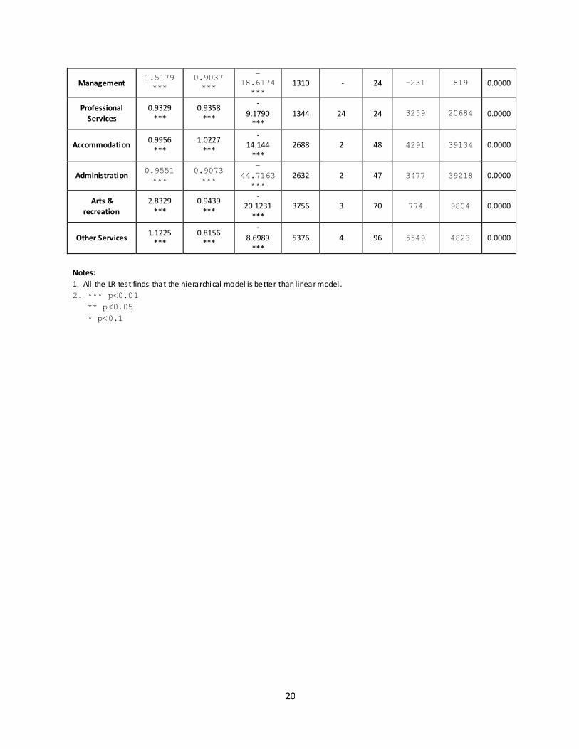
Table 1 presents the empirical results of equation (6). Starting from the third row of the
table, each horizontal row reports the regression coefficients for one model. The model results that test the all- industry aggregate data are presented the first and then the results for each individual industry sector (two-digit NAICS) are presented in turn.
The vector T(t): l_lnE captures the time effect. Based on correlograms, we identify that the source of panel specific serial autocorrelation for our data is basically from the first order autoregressive term. Shown in Table 1, the lagged time effect is statistically significant at the 0.01 level for the overall aggregate data as well as for data across all industries.
The overall establishment age effect (A) for aggregate data is not large (0.0744), but positive and statistically highly significant at 0.01 level. For each 1% increase in a Maryland county‘s average establishment age (in months), there is a 0.07% increase in the county‘s total employment, controlling for other factors. With the hierarchical modeling, the all- industry aggregate effect has incorporated the interrelationships of business age effects between each two-digit and three-digit NAICS sector and subsector.
For individual industries, the establishment age impacts are mostly highly significant as well, except for two sectors, Information (51) and Finance & Insurance (52). Among industries with a significant establishment age effect, more than half of the sectors display a positive establishment age effect. This means that for over half of industry sectors, older establishments is associated with a larger employment growth, controlling for other variables. This is particularly true with a coefficient of 0.20 or higher for Manufacturing (31-33) (0.1992), Wholesale Trade (42) (0.2726), Education Services (61) (0.2579), and Arts, Entertainment, and Recreation (71) (0.2428). Establishments in those sectors tend to have a relatively longer history and tends to be reputation based. Reputation needs time to build.
<Insert Table 1 here.>
However, for slightly above one third7 of the industry sectors— Agriculture, Forestry,
Fishing and Hunting (11), Mining, Quarrying, and Oil and Gas Extraction (21), Construction 7 8 out of 19.
11
(23), Utilities (22), Retail Trade (44-45), Real Estate and Rental and Leasing (53), Accommodation and Food Services (72), and Other Services (except for Public Administration) (81)—older establishments are associated with lower employment growth at the county level, holding other variables constant. Among those sectors, Construction (23) exhibited the most evident negative establishment age effect. For Construction (23) establishments, each 1% increase in a county‘s average establishments‘ age (in months) is associated with 0.63% decrease in the county‘s total employment, controlling for other factors. Establishments in Construction (23) tend to be small, volatile, and young. This on one hand gives them flexibility in catering for local consumer needs, on the other hand make them more vulnerable to the economic change. Many establishments in this sector that remain active for a long time do not increase employment much over time. Many of those establishments are also subject to seasonality. As time goes by, those establishments do not generate higher employment growth, and instead display a negative establishment age effect. Their momentum of employment growth is most likely to occur at the early stage of their business. Similar situation occurs to establishments, in Retail Trade (44-45), Real Estate and Rental and Leasing (53), Accommodation and Food Services (72), and Other Services (81). Those sectors also tend to be the ones hit severely by the recession. Sectors like Agriculture, Forestry, Fishing and Hunting (11) and Mining, Quarrying, and Oil and Gas Extraction (21) relatively have lower labor skill requirements and older infrastructures. For those sectors, older establishments do not necessarily have more mature skilled workers or a better business model; therefore, not necessarily generate more employment.
For the two unemployment rate measure, the magnitude of unemployment rates (U) does not exhibit a consistent effect on total employment and the effect is small; however, the differenced the unemployment rates (dU) shows a consistently negative and mostly highly significant effect (at 0.01 level) on county employment growth. This means that when unemployment rate trends up (i.e., during economic down turn), the county employment shrink three months later, holding other variables constant. While the magnitude of unemployment rate does not necessarily offer a straightforward impact on employment, the trend of unemployment rate changes matters. Only in three sectors, Utilities (22), Health Care and Social Assistance (62), and Management of Companies and Enterprises (55), the trend of unemployment rate does not seem to matter and result in a statistically insignificant effect. Those three sectors are also, relatively speaking, economically acyclical.
The results also show that the county population size is positively related to the employment growth. A larger size of population means a potentially larger labor pool for employment; it can also mean a larger consumer pool and thus a higher demand, which requires more employment as well. The positive population size effect is particularly evident in the sector of Administrative and Support and Waste Management and Remediation Services (56), according to Table 1. More residents in a county often mean more people to manage and administrate and immediately more personnel might be needed.
The average age of the county populations also display a positive effect. The county average age scales are all between age group value 7 and 9, corresponding to a range of age 30-44. Within this age range, the younger ones, those in early 30s could be more likely than those in 40s to be full- time or part-time students pursuing academic advancement instead of being full-time employees; early 30s are also tend to be the ages that are most bound by child caring responsibilities; compared toearly 40s. Within this age range, the higher the average age, a potentially higher labor force participation rate.
12
The racial diversity is an interesting variable in Table 1. Except for the sectors of Health Care and Social Assistance (62) and Professional, Scientific, and Technical Services (54), the coefficients of this variable are all negative if they are significant. As noted earlier, racial diversity as well as other population attributes from the Census Bureau are residential based, while employment data is workplace based. According to Table 1, Maryland counties with a higher residential racial diversity have lower employment growth, controlling for other variables. Some of the racial diversity effects are small, but for Manufacturing (31-33) and Real Estate and Rental and Leasing (53), there exist a large negative effect from racial diversity. Manufacturing (31-33) is a relatively old industry sector. Residential areas with a higher racial diversity level may tend to be relatively newer residential areas that attract new migrants and that might not have major manufacturing jobs available. Counties that have a higher residential racial diversity level have a higher proportion of minority residents. Many of the minority residents tend to be more vulnerable to employment and economic changes; this may help to explain the negative racial diversity effect on employment growth in many sectors. However, since minority is not an economically homogenous group, racial diversity would not be able to capture the full racial effect.
The gender ratio exhibits negative impacts on employment in many industry sectors, and positive impacts in several others. Most of the negative impacts are relatively small, compared to the positive impacts. The most pronounced gender effect is exhibited in Mining, Quarrying, and Oil and Gas Extraction (21). There is a a large and positive gender effect in this sector. It means that a higher proportion of male residents in a Maryland county, the higher total employment count in Mining, Quarrying, and Oil and Gas Extraction (21) in that county, controlling for other factors8. This sector is mostly concentrated in non-urban area and nonresidential areas where this sector is a major local job engine. Counties relying on Mining, Quarrying, and Oil and Gas Extraction (21) could be more concentrated with male laborers and with relatively limited female residents. In this case, there is a higher concentration of males, and a higher number of employed persons in this sector, controlling for other variables.
The regression diagnostics also show that hierarchical modeling is better than simple linear regression models, based on the likelihood ratio (LR) test. The hierarchical models using panel data captures both the overall establishment age and unemployment rate effects on employment growth, it also captures the interrelationship of establishments between three-digit NAICS industry codes, more general two-digit industry codes, and the county localities.
Appendix B exhibits the results of the earlier stage regressions during the multi-stage regression estimation process. Those results offer additional nuances. For most industry sectors, there seems to be a significant and positive establishment age impact on establishment size, but a significant and negative establishment age effect on establishment counts of a county. This means that when controlling for other factors, older establishments tend to be larger and have more employees for most industry sectors, except for the limited few with no statistical significance. Older establishments have been in business longer. According to the ―grow or out‖ principle in the business world, most of those older establishments have grown from smaller establishments years ago to larger establishments.
When holding other factors constant, counties with older establishments tend to have smaller numbers of establishments for all industry sectors but Education Services (61). Many 8 Please note again that the gender ratio is measured for residents and without distinction for industry sectors, while the employment is measured for workers with clear industry sector distinction. This situation made the interpretation of the gender ratio effect complex. At this moment, we can only try more evident exp lanations.
13
older establishments may have grown through merger and acquisition from other firms, which could shrink the total number of establishments. Since the relationship between establishment age and count is basically consistent across all industry sectors, industry mix seems not to be a deterministic factor resulting in this negative relationship. Education Services (61) becomes an exception possibly for two reasons. First, Education Services (61) tends to be a stable sector where majority of the establishments tend to last for a long time. This could include large educational institutions as well as small interest groups with special niche.
VI. Future Research Directions
This study delivers an exploratory analysis of the impact of business establishment age
on employment growth using reliable and recent administrative records. Future refinements, in addition to obvious interest in updating through the end of the recession and into the next growth phase, should include selected three-digit NAICS sector diagnostics.
Additional local labor force attribute data, versus population attribute data, are expected to be useful. The U.S. Census Bureau Longitudinal Employer-Household Dynamics (LEHD) Program longitudinal data files are likely to be the preferred choice for this refinement. Our next stage of analysis will respond to the multi- faceted challenges involved in grappling with merger, acquisition and other change-of-ownership events. This will refine our understanding of the complex relationship between business establishment age and firm age, as these have interdependent impacts on employment growth.
VII. Conclusions
Building on previous literature, this paper started with an economic accounting model
and then constructed a multi-stage regression model to estimate the business establishment age impact on employment growth. This multi-stage regression model inversely uses the traditional instrument variable techniques to directly test the elasticity of business establishment age on employment. This transforms business establishment age from an instrumental variable to a key explanatory variable. This methodology also considered the error term correlations among the seemingly unrelated regressions.
To explore the controversial role of business employment size, and overcome some previous limitations of business size and age measurement, we used longitudinal administrative data (QCEW data) to dynamically measure establishment age and size specific and current to each month when establishment employment was reported. This measure not only responds to the measurement timing challenge predecessors faced, but also uses a continuous measurement scale. Our business age and size measures also use county as the unit of analysis, instead of the traditional plant level. Using the county level data avoids plant level transitory business size class changes reported in previous studies, incorporates business birth and death related employment changes, measures the net employment growth in a regression model, and captures the local economic dynamics.
This paper relies on longitudinal administrative records, QCEW, with four data dimensions: time, county, two-digit NAICS code level, and three-digit NAICS code level. We therefore adopted hierarchical modeling techniques to capture the interrelationship between the different data dimensions. We also use panel data techniques to correct for location specific serial autocorrelations across time horizon.
14
Our analysis has shown that business establishment age is associated with local employment growth. In the all- industry-aggregate model, counties with older establishments exhibit a higher employment level, controlling for other variables. This is also consistent with the establishment age effect in over half of industry sectors. Therefore, for those industry sectors, targeting public assistance to older establishments could be more effective as a job growth strategy.
The establishment age effect on employment growth is not simply uni-directional across all industries. For over half of industry sectors, such as Manufacturing (31-33), Wholesale Trade (42, and Education Services (61), older establishments tend to have higher employment levels because scale, history, and reputation matter to them. Among other few industry sectors, such as Construction (23) and Other Services (81), investing in older establishments is less likely to be an effective employment growth strategy. For two sectors, Information (51) and Finance & Insurance (52), the establishment age effect is not statistically significant, and thus there is no direct evidence whether older establishments or newer ones contribute more to employment growth.
We measure unemployment rates with a differenced vector as well as a magnitude vector. Our findings show that the differenced vector exhibit a more consistent and deterministic effect than the magnitude measure. It is the trend of unemployment rate that matters, not the magnitude per se. When the monthly unemployment rates trend up, the county employment declines three months later in almost all industry sectors, except for three economically acyclical sectors—Utilities (22), Health Care and Social Assistance (62), and Management of Companies and Enterprises (55).
Our findings also reveal that for most industry sectors in Maryland counties with older establishments have a larger average establishment size and a smaller number of total establishments, holding other variables constant. We interpret this to mean that statewide employment growth policies are likely to be less efficient and effective as sub-state targeted policies that recognize the importance of differences in current local business size and age composition.
Unemployment?‖ Unpublished Working Paper. Available at http://www.bls.gov/opub/mlr/2000/07/art1full.pdf.
Bednarzik, Robert W. (2000), ―The role of entrepreneurship in U.S. and European job growth,‖ Monthly Labor Review, July 2000. Available at http://www.bls.gov/opub/mlr/2000/07/art1full.pdf.
Calvo, José L. (2006), ―Testing Gibrat‘s Law for Small, Young and Innovating Firms,‖ Small Business Economics, Volume 26, Number 2 / March, 2006 pp. 117-123.
Das, S., (1995), ―Size, age and firm growth in an infant industry: The computer hardware industry in India,‖ International Journal of Industrial Organization, Volume 13, Issue 1, March 1995, Pages 111-126.
Davidsson, Per, Lindmark, Leif and Olofsson, Christer, (1998), ―The Extent of Overestimation of Small Firm Job Creation – An Empirical Examination of the Regression Bias,‖ Small Business Economics, Volume 11, Number 1.
Davis, S. J., Haltiwanger, J. and Schuh, S. (1996), Job Creation and Destruction. The MIT Press.
Dunne, Paul and Hughes, Alan, (1994), ―Age, Size, Growth and Survival: UK Companies in the 1980s,‖ Journal of Industrial Economics, June 1994 Vol XLII.
Gibrat, R., (1931). Les ine´galite´s e´conomiques; applications: aux ine´galite´s des richesses, a` la concentration des entreprises, aux populations des villes, aux statistiques des familles, etc., d’une loi nouvelle, la loi de l’effet proportionnel. Paris: Librairie du Recueil Sirey.
Gibbs, J. P. and Martin, W. T. (1962). ―Urbanization, technology and the division of labor.‖ American Sociological Review 27: 667–77.
Haltiwanger, J. and Krizan C. J. (1999). ―Small Business and Job Creation in the United States: The Role of New and Young Businesses,‖ in Acs Z.(ed.) Are Small Firms Important? Their Role and Impact, Springer.
Hansen, John A., (1992), ―A Innovation, Firm Size, and Firm Age,‖ Small Business Economics, vol. 4(1), pp. 37-44.
Hart, P. E. (2000), ―Theories of Firms' Growth and the Generation of Jobs,‖ Review of Industrial Organization, Volume 17, Number 3 / November, 2000
Kaplan, D.S. (2003), ―Worker- and job-flows in Mexico,‖ working paper. Available at http://www.iadb.org/res/laresnetwork/projects/pr191finaldraft.pdf.
Persson, H. (2004), ―The Survival and Growth of New Establishments in Sweden, 1987-1995Small Business EconomicsVolume 23, Number 5 / December, 2004, 423-440
Reynolds, Paul D., (1997), ―New and Small Firms in Expanding Markets,‖ Small Business Economics Volume 9, Number 1 / February, 1997 79-84.
Stiglbauer. Alfred, Stahl, Florian, Winter-Ebmer, Rudolf and Zweimüller, Josef, (2003), “Job Creation and Job Destruction in a Regulated Labor Market: The Case of Austria,‖ Empirica, Volume 30, Number 2 / June, 2003.
Wagner, J. (1997), “Firm Size and Job Quality: A Survey of the Evidence from Germany?‖ Small Business Economics, Volume 9, Number 5 / October, 1997
Wren, Colin, (1998), ―Subsidies for Job Creation: Is Small Best?‖ Small Business Economics, Volume 10, Number 3 / May, 1998, pp. 273-281.
Zellner, A., (1962), ―An Efficient Method of Estimating Seemingly Unrelated Regressions and Tests for Aggregation Bias,‖ Journal of the American Statistical Association, 57: 348-368.


![Civilian Employment and Unemployment by Sex and Age...TABLE C-23. Civilian employment and unemployment, by sex and age, 1947-69 [Thousands of persons 16 years of age and over] Year](https://static.documents.pub/doc/80x56/60a4eac7a2be892e351fbc31/civilian-employment-and-unemployment-by-sex-and-age-table-c-23-civilian-employment.jpg)


