Working Paper Series _______________________________________________________________________________________________________________________ National Centre of Competence in Research Financial Valuation and Risk Management Working Paper No. 479 Business and Financial Indicators: What are the Determinants of Default Probability Changes? F. Couderc O. Renault O. Scaillet First version: April 2007 Current version: April 2007 This research has been carried out within the NCCR FINRISK project on “Financial Econometrics for Risk Management” ___________________________________________________________________________________________________________
Keywords: censored durations, proportional hazard, business cycle, default
determinants, default prediction.
ABSTRACT
This paper investigates some common determinants of default probability changes ofindividual firms using Standard & Poor’s ratings database. We analyze and quantify the re-sponses of hazard rates to changes in various economic variables, namely financial markets,business cycle and credit indicators, and examine their persistency. First, we show that in-cluding non-financial information largely improves the poor explanatory power of financial-based factor models. More importantly, in comparison with market factors, business andcredit factors become dominant as the issuer quality decreases. Second, we highlight thebenefits of past information. Our results prove that both past shocks and subsequent eco-nomic trends are of prime importance in explaining probability changes. To draw theseconclusions, we introduce a semi-parametric framework accommodating the continuous na-ture of probability changes and ageing effects. It allows us to recover default probabilitiesover any desired time horizon.
∗Swiss Finance Institute at University of Geneva, Bd du Pont d’Arve 40, 1211 Geneva 4, Switzerland.†Associate Fellow, FERC, Warwick Business School, Coventry CV4 7AL, UK.‡Swiss Finance Institute at HEC-University of Geneva, Bd du Pont d’Arve 40, 1211 Geneva 4, Switzerland.§The authors gratefully acknowledges data support by Standard & Poors. In addition the first author thanks
financial support from the Swiss National Science Foundation through the National Center of Competence:Financial Valuation and Risk Management (NCCR FINRISK) and from the Geneva Research CollaborationFoundation (GRC). We thank Arnaud de Servigny, Ren Stulz, Laurent Barras, anonymous participants tothe 2005 GRETA Credit conference and members of Standard & Poors European academic panel for usefulcomments. The views expressed therein are those of the authors but not necessarily those of Standard & Poorsor any other institution. All remaining errors are ours. Corresponding author: F. Couderc, [email protected].
1
Introduction
Understanding and modeling the common dynamics of default probabilities is a key concernfor practitioners and academics. Probability changes have a significant impact on the pricesof credit risky instruments but also on the way credit risk should be managed. Regulationissues especially through economic capital computations, as well as large variations in defaultrates over the last five years have renewed interest in this topic. Common dynamic changesin probabilities have mainly been investigated using historical rating migration matrices or,from pricing perspectives, by modeling credit quantities (in particular credit spreads). It turnsout that significant differences in probability levels have been observed through expansion andrecession periods (e.g. Nickell, Perraudin and Varotto 2000).
Researchers have concentrated on modeling and forecasting these changes either by filteringout unobservable common drivers (see e.g. Duffee 1999 or Driessen 2005 under the pricingmeasure, Koopman, Lucas and Monteiro 2008 or Wendin and McNeil 2006 under the historicalmeasure) or using stock and bond markets factors (Janosi, Jarrow and Yildirim 2002). Theseapproaches find their origins in structural models (firm-value based) and reduced-form models(intensity based). The former are closely linked to financial markets as they model defaultas the first time at which a firm asset value falls below its liabilities. But they regularly failto provide accurate probability estimates. This is essentially due to structural models heavilyrelying on stock market components which are noisy and contain bubbles, as pointed out byJanosi et al. (2002). Another reason for this failure is that some parameters, such as theasset volatility, are difficult to observe and calibrate. The intensity-based methodology is moreconvenient for pricing and provides simple extensions to multiple assets (e.g. see Duffie andSingleton 2003).1 However, since dynamics are exogenously specified, this approach ignoreswhat the default mechanisms are and leads to disappointing predictive power as well. It isworth noticing that firm-specific variations have also been documented. This last stream ofstudies relies on different modeling techniques, namely credit scoring or hazard rate models(see e.g. Duffie et al. 2007) which will be used in this paper.
A key issue lies in the identification of the systematic drivers of default probabilities. Somestudies observed surprisingly low sensitivities of spreads to interest rate factors or to stockmarket variables (see e.g. Collin-Dufresne, Goldstein and Martin 2001), but explanations arelacking. This paper contributes to the existing literature by considering a new set of potentialdeterminants that explicitly link the default process to economic fundamentals. This studyshows that including all economic components provides more accurate measures than those
1We will abusively use indifferently the terms of hazard rates and intensities in this paper. We will onlypoint out the differences when outlining our framework.
2
obtained from financial market factors. For the first time, the critical roles of business cyclerelated indicators as well as aggregate credit market factors are identified and quantified. Anadditional contribution lies in the use of past information, jointly with contemporaneous one.We show that large benefits can be obtained by taking into account lagged effects between theeconomy and the default cycle. The empirical part of the paper relies on a unique rating eventdatabase that captures more precisely the default probabilities, whereas the previous body ofevidence is based on a noisy measure of these probabilities, namely the credit spreads.
We believe there are four main contributions of this paper. First, we analyze and quantifythe impact of financial markets, business cycle indicators and credit market indicators on de-fault probabilities of various rating classes.Second, we show that although all economic variables help explaining default likelihoods, theirexplanatory power differs greatly between investment- and noninvestment-grade classes. Asissuer quality decreases, the dominant systematic factors change from financial markets to busi-ness cycle and endogenous default indicators. Relying solely on financial information to explaindefault probabilities leads to poor results for noninvestment-grade firms. Default peaks areunderestimated whereas default probabilities predicted by the model overshoot realized prob-abilities during stable and low-default periods.Third, we establish the critical importance of combining past information with contemporane-ous factors. We show that default probability changes are the joint effects of past shocks andsubsequent economic trends. Resulting lead-lag effects between the economy and the defaultcycle partially explain the lower speed and higher persistence of the default cycle.Fourth, we introduce a semi-parametric framework which explicitly takes into account theterm structure of hazard rates. Firm ageing effects as well as calendar-time effects are explic-itly taken into account. Models are set up in continuous time using the natural time-to-defaultframework and taking care of censoring. In particular, default probabilities can consistentlybe computed at all horizons. A specification test is also introduced.
The paper is organized as follows. The first Section briefly present the default data. Section2 presents our modeling framework. We then propose a list of potential default determinantswhich will be investigated in later sections. We extensively study sensitivities of the defaultcycle with respect to financial markets, business and endogenous indicators through conditionalsingle factor hazard models in Section 4. Section 5 gathers main results and their implicationslooking at multifactor models. We check misspecifications of financial market based models,and assess the benefits of considering other economic components. Our results deliver clearempirical guidelines for modeling. They rely on analyzes of predictive variables of defaultprobabilities exploiting the history of companies in the rating process. This study opens newavenues to investigate the intensity-based pricing and the management of default risk. It more
3
particularly sheds light on relevant systematic factors for the construction of realistic stresstests of credit portfolios in the Basel II framework.
1. Default Dataset
We extract information on times-to-default from the Standard & Poor’s Credit Pro 6.6 ratingdatabase. As the first goal of ratings consists of providing a cross-sectional ranking of firmswith respect to their default likelihood, they allow to classify firms into ”homogenous” classesof default risk. The database contains S&P’s rating histories for 10439 companies over theperiod January 1981 to December 2003. The Credit Pro database has already been usedand extensively described by Bangia et al. (2002) and Couderc (2005). Overall 33044 ratingmigrations are recorded in CreditPro as well as 1386 defaults and default rate ranges from3% to 29% across industries. Within our sample, firms are classified by industrial groupsdistributed among 93 countries. 6897 firms or 66% are US ones. Moreover, S&P attributes25 distinct ratings plus the not-rated one (NR) one, but we aggregate the data coming from agrade and its plus/minus modifiers because of minimal population requirements. Besides, allgrades below B- have been put in the CCC class.
Rating events require careful treatment as three sources of censoring are present in thedatabase. The first type of right censoring is an inherent feature of any rating database asmost companies survive after the end of the recordings. Another type of right censoring requiresspecific consideration. Some companies leave the rating process and fall into the NR category.Several reasons may explain this fact: the rated company may be acquired by another firm ormay simply decide no longer to be rated by S&P. In the database we can identify firms thatmigrated to NR and subsequently defaulted. Therefore the NR class is not a complete loss ofinformation: although there is no longer any indication of credit quality, a NR firm is a nondefaulter. Finally, left censoring arises from 1371 issuers having already received a rating beforethey were included in the database (i.e. before January 1981). We do not have informationabout the attribution date of their first rating and therefore, for robustness checks, we run allestimations both on the full sample and on the reduced sample excluding left-censored data(the reduced sample contains 9068 companies and 25993 rating migrations). It is worthwhileto notice that these left censored issuers faced the 1991 and 2001 US recessions. The number ofissuers tracked by the database increases linearly. Consequently, one third of the total numberof issuers were active on average since 8 years in 1991 and 18 years in 2001, and another onethird only faced the 2001 recession after an average of 4 years in the rating process.
4
The database allows to consider two types of durations, implying two different approachesto the behavior of default probabilities. On the one hand, we can look at times-to-default fromentry in a risk class up to the last available observation. Such durations provide a picture ofdefault riskiness over the whole life of the firms without any assumption on the rating processbehavior. On the other hand, we can examine times-to-default conditional on staying in agiven risk class up to the default time. In this case, it would require assumptions on ratingmigration dynamics so as to design the default riskiness of a firm over the long term.
2. Models of Default Probabilities
Hereafter we develop a powerful framework to analyze impacts of systematic factors. Astraightforward practice to study the effects of structural factors on a given variable consistsin performing regressions. Investigations of spreads follow this approach but it cannot be usedfor probability changes because hazard rates or equivalently instantaneous default probabilitiesare not directly observable. Since hazard rates fully characterize a default time distribution,modeling hazard rates leads to specifying the conditional distribution of times-to-default, andall parameters can be estimated in a single stage. We rely on the standard way to constructhazard models, with log-intensities that are linear in the factors. We briefly recall the basicparametric framework before turning to our more complete semi-parametric framework.
2.1. Factor Models of Intensities
For a firm i in a given risk class, let Di denote the uncensored duration up to default, ortime-to-default, and Ci the censored duration. Ui = min (Ci, Di) is the time at which the firmleaves the class either because of censoring (Ci) or default (Di). The Ui are therefore the trueobservations. We also let Z and u denote respectively a vector of explanatory variables andthe time-to-default or ageing time, while ti denotes the date at which a firm i enters into theclass. Hence, u + ti represents calendar time. We consider intensities λi as exponential affinefunctions which remain constant between two observations of the factors. Conditional on therealization of the factors, durations are exponentially distributed between factor updates:
λi (u) = λ (u, ti) = exp(γ + β′Z (ti, u + ti)
) ∀i, (1)
where Z can include a combination of time-dependent and time-independent covariates. Theexponential assumption could be relaxed by replacing the constant exp (γ) by another for-mulation. For instance, one could impose a conditional Weibull hazard model. The survival
5
probability for a firm i beyond the time u + ti can then be retrieved as P (U > u| ti) =exp
(− ∫ u0 λ (u, ti) du
).
This parametric framework allows us to use maximum likelihood to efficiently estimate β.Details of maximum likelihood estimation in this context are provided in Appendix. The esti-mation of such models is therefore straightforward and both censored and uncensored durationscontribute to the likelihood.
The accuracy of the above estimator depends on the proper specification of the model, onthe selection of explanatory variables and on time-to-default being conditionally exponentiallydistributed. However, some empirical studies have demonstrated that these simple modelsare misspecified even if they successfully take into account all systematic factors. Fledeliuset al. (2004) and Couderc (2005) have shown that economic changes create bumps in hazardrates and have established that the distribution of times-to-default is not exponential (i.e.the hazard is not constant with u). In the remainder of this paper we propose to use asemi-parametric framework for hazard models which relaxes this exponential assumption. Thenonparametric component of these models allows us to extract the baseline hazard, which is thetrue conditional distribution of times-to-default which characterizes the whole term structureof hazard rates. The parametric part of the models reflects shocks to the hazard rates dueto changes in economic and financial factors. Once these shocks have been accounted for, theremaining bumps in the baseline hazard indicate the proportion of the default cycle which isnot captured by the factors. If the factors were able to fully describe the patterns of historicaltimes-to-defaults, then the baseline hazard would be constant and we would fall back on theclass of simple models described above.
2.2. A Semi-Parametric Framework for Intensities
In our semi-parametric setting, calendar time effects, or factor impacts, can easily be separatedfrom pure duration or ”life cycle” effects on hazard rate deformations. To build our setup westart from a fully nonparametric estimator of hazard rates and add a multiplicative parametriccomponent (Cox 1972 1975 proportional hazard methodology). The nonparametric baselinehazard is estimated using the GRHE (Gamma Ramlau-Hansen Estimator) as the solution ofthe maximum likelihood objective function, while the parametric part is estimated by partiallikelihood.
6
2.2.1. The Basic Estimator
The GRHE introduced by Couderc (2005) is based on a convenient Gamma kernel smootherof the hazard rate and allows to recover the term structure of hazard rates. Standard smoothestimators suffer from large bias and oversmoothing, which lead to incorrect inferences onhazard rates. The GRHE however is free of boundary bias and is able to capture changes inintensities in the short run (which may cover up to 5 years) as well as subsequent deformations.2
Not using an unbiased estimator would lead to strongly inaccurate estimations and assessmentsof hazard models.The necessary conditions ensuring the consistency of the estimator are assumed to be met.Accordingly, all firms in a given risk class are assumed to be homogenous and conditionallyindependent. Censoring mechanisms which may prevent from observing firms up to theirdefault time are random and independent from the default process. For a given firm, thesemechanisms are reported through a process Y i (u), which equals one only if the firm wasobserved at least up to the time-to-default u. The most important building block of theGRHE then lies in the following assumption :
Assumption 2.1 The intensity of individual firms satisfies the Multiplicative Intensity Model:
λi (u) = α (u) Y i (u) (2)
where α (u) is deterministic and called the hazard rate whereas Y i (u) is a predictable andobservable process.
The difference between the intensity and the hazard rate resides in their observability. Theestimator of the hazard rate is specified as:
Definition 2.1 The gamma kernel estimator α (u) of the hazard rate (Gamma Ramlau-HansenEstimator, GRHE) is defined by
α (u) =
∞∫
0
1Y (s)
su/b e−s/b
bu/b+1 Γ(
ub + 1
)dNs , (3)
where dNs counts the number of defaults occurring at time s and Y (u) is computed as thenumber of firms for which the last time of observation is greater than u.
2This feature has already been widely documented in the case of density function estimation. Standardsmoothers are biased because of the inadequacy between the domain of definition of the kernel and the one ofthe data. For instance, see Chen (2000).
7
Y (u) handles censoring and is the sum of the Y i (u) over i. It is usually called the risk set. b is asmoothing parameter, the so-called bandwidth. The intuition behind the above nonparametricestimator is the following: probabilities of default in the very short run (α (u) du), knowingsurvival up to time u, are estimated as a weighted average of past (if any), current andsubsequent observed instantaneous default frequencies ( dNs
Y (s)). The weights are determinedby the kernel, the bandwidth, as well as by the durations between u and observed defaultevents.The restrictions imposed on the process Y (u) are sufficiently weak to permit more complexspecifications of this process. In what follows, we rely on this multiplicative intensity model,to characterize economic shocks on time-to-default distributions.
2.2.2. Factor Models for the Term Structure of Hazard Rates
Let Z denote a vector of factors. We enrich standard factor models of hazard rates from section2.1 by relaxing the conditional exponential assumption, or equivalently by not constrainingthe term structure of hazard rates. This is done by using a semi-parametric framework. Asdiscussed previously the parametric part reflects the impact of economic and financial factors ondefault intensities, whereas the baseline hazard or conditional distribution of times-to-defaultis estimated through a slight modification of the GRHE.
Assumption 2.2 The intensities conditional on structural factors are proportional to a classbaseline intensity λ◦ (u) representing the common intensity shape:
λ (u, ti) = λ◦ (u) exp(β′Z (ti, u + ti)
) ∀i (4)
= α◦ (u) Y i (u) exp(β′Z (ti, u + ti)
) ∀i
where Z (ti, u + ti) is the set of structural variables taken at the date of entry ti of the firm i inthe class or at calendar time u + ti, and β is the vector of sensitivities associated with a givenrisk class.
Provided that structural variables dynamics are not explosive, the Gamma kernel estimatorof the baseline hazard α◦ (u) becomes:
8
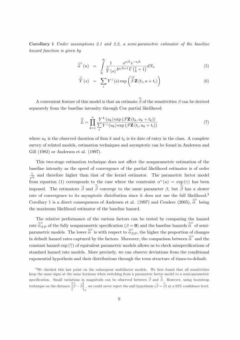
Corollary 1 Under assumptions 2.1 and 2.2, a semi-parametric estimator of the baselinehazard function is given by
α◦ (u) =
∞∫
0
1Y (s)
su/b e−s/b
bu/b+1 Γ(
tb + 1
)dNs (5)
Y (s) =
∑
i
Y i (s) exp(
β′Z (ti, u + ti)
)(6)
A convenient feature of this model is that an estimate β of the sensitivities β can be derived
separately from the baseline intensity through Cox partial likelihood:
L =
n∏
k=1
Y k (uk) exp (β′Z (tk, uk + tk))∑i
Y i (uk) exp (β′Z (ti, uk + ti))(7)
where uk is the observed duration of firm k and tk is its date of entry in the class. A completesurvey of related models, estimation techniques and asymptotic can be found in Andersen andGill (1982) or Andersen et al. (1997).
This two-stage estimation technique does not affect the nonparametric estimation of thebaseline intensity as the speed of convergence of the partial likelihood estimator is of order1√n
and therefore higher than that of the kernel estimator. The parametric factor modelfrom equation (1) corresponds to the case where the constraint α◦ (u) = exp (γ) has been
imposed. The estimators β and β converge to the same parameter β, but
β has a slowerrate of convergence to its asymptotic distribution since it does not use the full likelihood.3
Corollary 1 is a direct consequences of Andersen et al. (1997) and Couderc (2005), α◦ beingthe maximum likelihood estimator of the baseline hazard.
The relative performance of the various factors can be tested by comparing the hazardrate α◦NP of the fully nonparametric specification (β = 0) and the baseline hazards α◦ of semi-parametric models. The lower α◦ is with respect to α◦NP , the higher the proportion of changesin default hazard rates captured by the factors. Moreover, the comparison between α◦ and theconstant hazard exp (γ) of equivalent parametric models allows us to check misspecifications ofstandard hazard rate models. More precisely, we can observe deviations from the conditionalexponential hypothesis and their distributions through the term structure of times-to-default.
3We checked this last point on the subsequent multifactor models. We first found that all sensitivitieskeep the same signs at the same horizons when switching from a parametric factor model to a semi-parametric
specification. Small variations in magnitude can be observed between β andβ. However, using bootstrap
technique on the distance
∥∥∥∥β − β
∥∥∥∥2
, we could never reject the null hypothesis (β =β) at a 95% confidence level.
9
3. Potential Determinants of Default
In this section, we discuss some potential common determinants of default intensities that willbe tested in our model. Mainstream models that attempt to explain risk-neutral default prob-abilities are usually calibrated on financial variables: interest rates and equity information.Another stream of literature focuses on long-term economic and credit cycles and relies mainlyon macroeconomic variables to explain default rates. The business cycle has for example beenfactored in time series analyzes of procyclicality with the bankruptcy cycle (e.g. see Koopmanand Lucas 2004). To our knowledge, there exists no systematic study of the common deter-minants of default including both financial and non financial variables, and we will attemptto fill that gap here. Given that our sample is primarily American, we use US explanatoryvariables. Our economic data was extracted from the Federal Reserve of St. Louis web siteand Bloomberg. All factors are annualized, deseasonalized and updated monthly or quarterly.
3.1. Financial Market Information
The stock and bond markets are sources of information used both by structural (i.e. firm-value based, la Merton) and reduced form models. Reduced form models typically require todesign a stochastic process of interest rates. For instance, Duffee (1999) relies on a two factorinterest rate model to extract default intensities. In a structural approach, the volatility andreturn of the firm asset determine how close a firm is to its liability barrier which representsthe default threshold. Cremers et al. (2006) show that individual stock return and volatilityare significant determinants of spreads. Using an aggregate measure, Janosi et al. (2002) andCollin-Dufresne et al. (2001) also establish the impact of respectively the S&P500 index andthe VIX on credit spreads. The latter further claim that using individual stock volatility ratherthan index volatility does not modify their results. We consequently test the following factorson hazard rates:
- Annual return on S&P500: as a measure of asset levels, the higher the stock return, the higherthe distance to default should be. An increase in equity prices tends to decrease firmleverage and therefore pushes down default probabilities. Moreover, from an economicstandpoint, short- and mid-term economic performance should be positively correlatedwith S&P500’s returns. We expect a negative impact on default intensities (i.e. intensitiesshould be a decreasing function of the factor).
- Volatility of S&P500 returns: in a traditional Merton (1974) -type model, the two drivers ofdefault probabilities are leverage and the volatility of firms assets. The implied volatility
10
of equity returns is often used as a proxy for the latter. We use the realized annualizedvolatility computed over 60 trading days. We expect it to have a positive impact ondefault intensities.
- 10-year treasury yield: higher interest rate levels imply higher cost of borrowing. Hence, thisvariable could impact positively on default probabilities. However interest rates tendto be lower in contraction periods and higher in expansions. The ultimate impact onintensities is therefore uncertain and may depend on issuer quality.
- Slope of term structure (10-year rate minus 1-year rate): steep term structures of interestrates are usually associated with strong growth prospects. It can also reflect expectationsof higher future spot rates. We expect this variable to impact negatively on mid- to long-term intensities.
3.2. Business Cycle
We believe that it is crucial to extract information from the business cycle. If stocks wereavailable for all firms and markets were fully efficient, financial market and business cyclevariables might be redundant. As mentioned, the return on the market index does not con-stitute a perfect proxy for the state of the economy. To complement financial variables, Fons(1991) regresses default rates on the GDP growth, and Helwege and Kleiman (1997) add theNBER economic indicator. These business cycle indicators explain 30% of the annual defaultprobabilities. We will use these variables in our estimations and will also include the personalincome growth as Duffie et al. (2007).
- Real GDP growth: as a signal of current macro-economic conditions this variable should benegatively correlated with short term probabilities.
- Industrial production growth: this is an alternative growth measure which should have asimilar impact as that of GDP growth. Its advantage over GDP growth is that it offersmore frequent updates (monthly vs. quarterly).
- Personal Income Growth: same expected impact as the previous two variables. This businessfactor is more volatile and should consequently be less persistent. This indicator couldalso convey some slightly lagged information on past business conditions.
- CPI growth: inflation is again a general indicator of economic conditions. We expect toobserve a negative correlation with short term default probabilities, as high inflation hasoften been associated with growth.
11
3.3. Credit Market Information
In addition to general economic variables and financial information, more specific credit factorsshould prove valuable in explaining default intensities. Although corporate bond spreads do notonly reflect changes in underlying default probabilities (see e.g. Ericsson and Renault 2006),they should still contain some forward-looking information on default probabilities. Moreover,when spread variations are due to changes in the default risk premium, they involve changes inexpectations of future economic conditions. Spread factors may therefore be more persistentthan other market factors.
- Spread of long term BBB bonds over treasuries: they reflect future default probabilities, ex-pected recoveries as well as default and liquidity premia. It should therefore be positivelycorrelated with default intensities.
- Spread of long term BBB bonds over AAA bonds: this variable factors in the risk aversionof investors and may be a measure of their risk forecast. It filters out mixed effectscontained into the BBB spread. Furthermore, an increase in the relative spread mayreflect an increase in firms asset volatilities (see Prigent et al. 2001). We thereforeexpect default intensities to increase with this variable.
- Net issues of Treasury securities: this indicator should positively impact short term proba-bilities of default as higher deficit and borrowing is an indicator of economic difficulties(it is at least negatively correlated with the business cycle). Furthermore, high publicsector borrowing may crowd out private borrowers and lead to increased financial diffi-culties for firms. However, if borrowing is used for investments, an increase in Treasuryissuance may be linked to stronger growth in the long term and decreasing probabilitiesof default.
- Money lending (M2-M1) and bank credit growth: these factors measure credit liquidityand should be associated with default intensities. It is well known that the informationcontent of this indicator and more particularly of M2 has changed a lot over our sampleperiod (series of adjustments have been done by the Federal Reserve). As a consequence,this indicator cannot be conclusive in the short run, but its implications in the long runturn out to be fairly stable. We thus expect clearer impacts when using lags.
3.4. Inner Dynamics of the Default Cycle
A striking feature of the default cycle might not be captured by the above variables. Afterthe last two recessions strong persistence in default rates has been observed. The number of
12
defaults remained high even during economic recoveries. The default cycle seems to exhibit itsown dynamics. We believe that the set of predictive variables should be expanded with default-endogenous variables. Kavvathas (2000) used the weighted log upgrade-downgrade ratio andthe weighted average rating of new issuers as explanatory variables. He actually only took intoaccount the first PCA factor of these variables. The average rating of financial institutions maybe of primary interest in describing the short term trend of the global economy (in terms ofcredit crunch). This trend can also be captured by the ratio of downgrades over all non-stayertransitions. For instance, Jonsson and Fridson (1996) show that the credit quality of speculativeissuers explains a large proportion of annual aggregate default rates. As representative of thedefault cycle trend we choose to include the following rating-based variables:
- IG and NIG upgrade rates : both variables should include information on economic health.4
- IG and NIG downgrade rates : downgrades should be higher in bad conditions. Differencesbetween upgrade and downgrade impacts should capture a potential asymmetry in thedefault cycle.
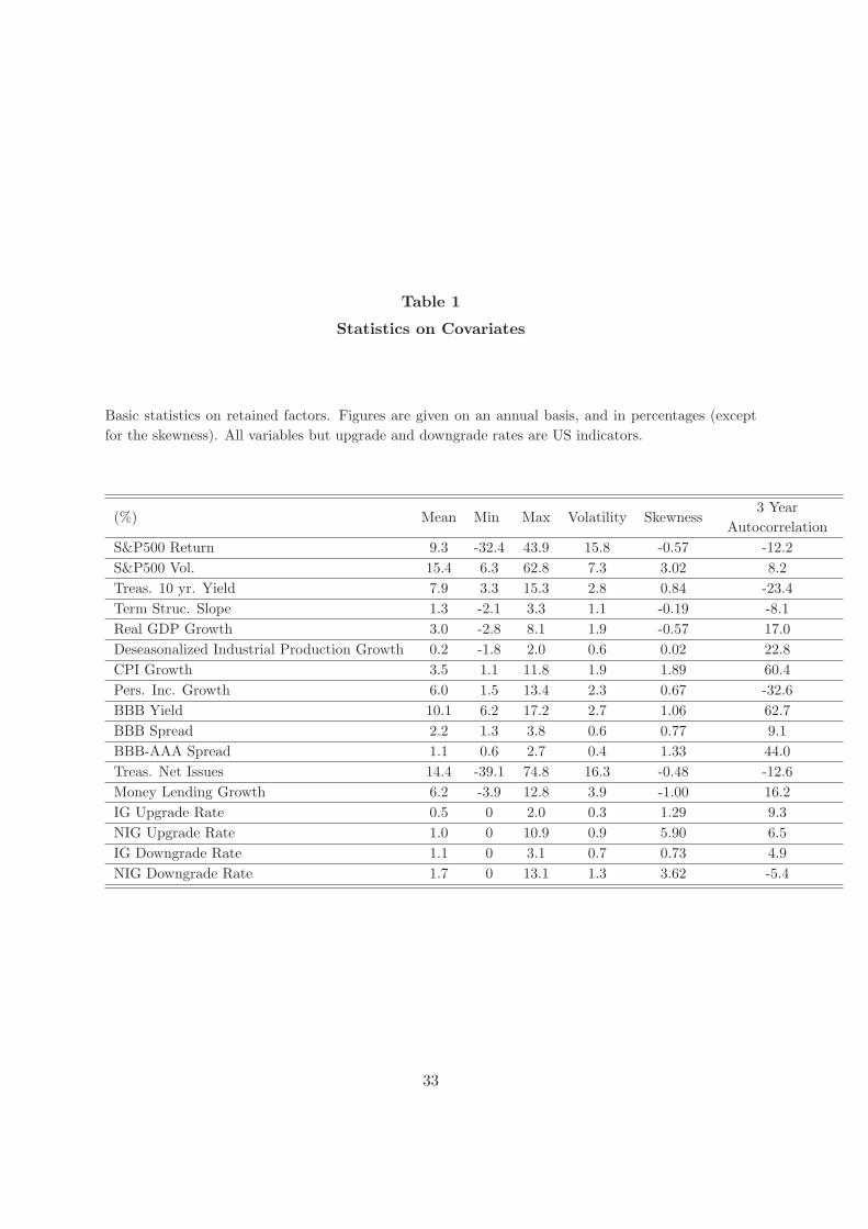
3.5. Statistics
Table 1 presents basic statistics on the set of retained factors. Obviously some of the abovevariables such as real GDP growth and industrial production growth are highly correlated,which would deteriorate statistical significance on the full set of variables. Many of thesefactors are redundant, and will be eliminated at the estimation stage in multifactor analysis.Taking a pragmatic approach, we will first identify the most relevant factors and then constructparsimonious multifactor models.
[INSERT TABLE 1 HERE]
Although we do not explicitly include firm-specific factors, our approach does not fullyrule out non systematic risk as we will examine rating classes separately. Ratings shouldindeed constitute stable and good proxies for firm-specific components and a fair alternativeto specific variables, which are not always available or are not updated frequently. Leveragetargeting, jointly with the way ratings are reviewed, justifies this point. From an accountingperspective, default cannot realistically be initiated by small changes in earnings, leverage orany balance sheet information but rather by negative trends or by unexpected large changes
4The investment-grade class (IG) gathers the AAA, AA, A and BBB classes whereas BB, B and CCC classesare collected in the noninvestment-grade (NIG) class.
13
in cash flows. Any negative trend should have been incorporated in issuer ratings. One mayargue that ratings do not react quickly enough to new information, but there is no consensuson this issue (see Altman and Rijken 2004 or Loffler 2004) and we will assume that ratingscapture significant changes in firm-specific components.
4. Predictors and Indicators of the Default Cycle
In this section, we investigate time-dependent covariates which embed the impact of successiveshocks of the economic environment on intensities: when the factor updates, hazard rates areshifted and the conditional distribution of times-to-default is updated too. We distinguish theimpacts of current and past economic conditions on default time distributions. We examinethe sensitivity of hazard rates to each factor in order to determine which factors are the mostrelevant. We also explore their persistency. Surprisingly, the issue of lagged information hasbeen ignored in most papers on default probabilities, although Koopman and Lucas (2004)have reported lagged effects between the market and the bankruptcy cycle.We analyze the explanatory power of each factor through maximum likelihood estimations.For each covariate we run distinct lagged estimations to examine the persistency of its effects.In all cases, we look at 95% and 99% confidence tests, and likelihood ratios. The alternativemodel of the likelihood ratio test corresponds to unconditional exponentiality, i.e. the case ofconstant intensity. We also break our dataset into several samples, namely investment-grades(IG), noninvestment-grades (NIG), AA, A, BBB, BB, B and CCC samples.
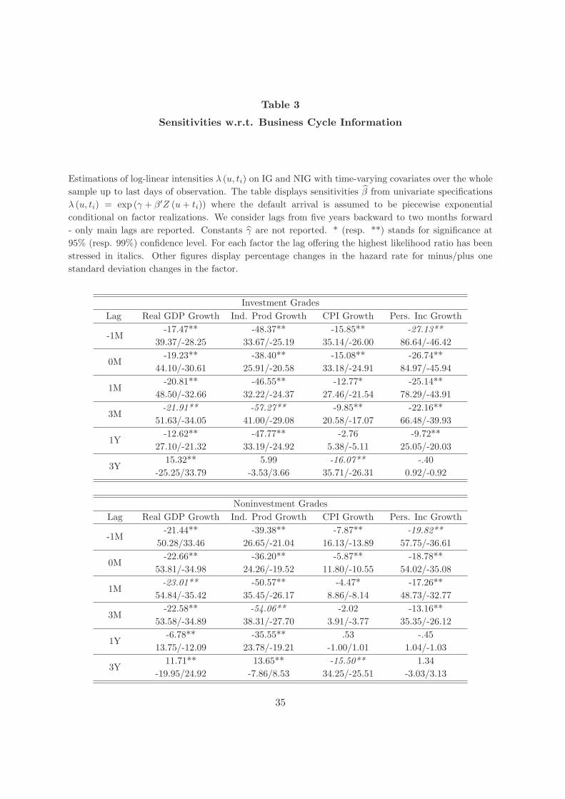
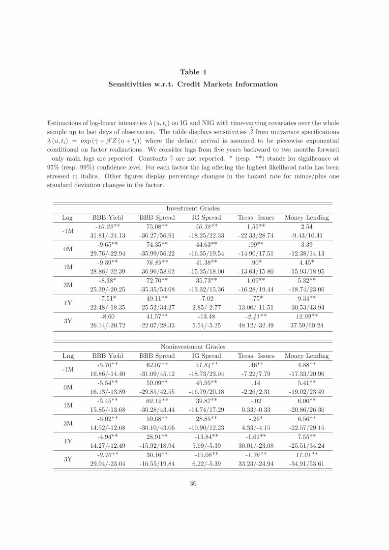
Tables 2, 3 and 4 present results on the broad IG and NIG samples respectively overfinancial, business and credit indicators. In addition to sensitivities, implied percentage changesin the hazard rates are provided when the factor changes by minus or plus one standarddeviation. These changes are not symmetric as the factor impacts the hazard rates throughthe exponential function. Table 5 reports estimates of sensitivities with respect to upgrade anddowngrade rates over rating classes. To test the stability of the results we have estimated themodels on various sub-samples and found that the sample used makes little difference in mostcases. For example, considering durations up to the first exit from a risk class (rather thandefault) keeps sensitivities almost unchanged and only lowers the significance of parameters.Focusing solely on the US sub-sample does not modify our estimates by more than 10% onaverage, and does not alter signs. Such robustness could be expected as risk classes are quitestable and the whole sample is made of 66% US firms. From a general perspective, all includedvariables are significant. We observe that most lagged factors are significant at all stages too.In addition, these findings do not change across ratings. Estimated intercepts (γ) lie around
14
-13.1 for IG and -8.8 for NIG. Results on lags between two to five years are similar than theones of the three-year lagged factors. These results are not reported here.
4.1. Influence of Financial Markets
[INSERT TABLE 2 HERE]
Table 2 shows that financial markets impact default probabilities as predicted by structuralmodels (lags up to three months). Increases in the market index decrease the probability ofdefault while increases in volatility raises default probabilities. Increases in long term interestrates are good news because they reflect growth expectations. These findings are consistentwith the results of Duffee (1998) and Collin-Dufresne et al. (2001) on spreads.
Unlike the above authors, we find that the slope of the term structure is significant andhas a large effect on hazard rates. In particular, Collin-Dufresne et al. show a significantand negative relationship only with long maturity bonds with reasonable leverage, whereas itbecomes positive for short maturities. Table 2 explains this result. Decreases in short termyield raise default probabilities as low rates are strongly correlated with recessions. A steepcontemporaneous or recent slope of the term structure of riskless rates tends to be associatedwith higher intensities of default while past steep slopes (over one-year lags) tend to decreaseintensities. Therefore, effects on bond spreads are the results of these conflicting phenomena,which dampens significance. Short maturity bonds are mainly affected by recent changes inslope, so that an increase in the slope leads to an increase in hazard rates and spreads. Theonly exception to this short term/long term interest rates split is for the CCC class, for whicha steep slope is always associated with lower intensities, irrespective of the lags. This can bedue to two reasons. First, low short-term interest rates can indicate a slowdown of economicactivity and an increased competition in the corporate bond market. Second, increases in longterm interest rates are often interpreted as expectation of higher growth. Future growth isthe main determinant of survival for junk issuers, as these companies are highly levered andrequire strong business conditions to move up the rating ladder.
Some of the studies of corporate bond spreads mentioned above indicate a higher impactof the market index than interest rates. Looking at implied percentage changes on the hazardrate, our results are more contrasted. For investment grades, a decrease in the long term yieldand an increase in the slope lead to shocks of the same order of magnitude than a decrease inthe S&P500 return. Even if all market indicators have smaller effects on NIG, contemporaneouschanges in the slope have lower impacts than changes in the S&P500 return, and impacts ofthe market index are a bit more persistent. It may explain why interest rates have usually been
15
found to be less economically significant. The results on the impact of volatility are interestingand challenging for the structural models a la Merton on an aggregated pool of firms. Weindeed find that volatility has a lower impact on hazard rates for noninvestment-grade firms,which is the opposite of what is predicted by structural models. We will come back to thispoint later on.
4.2. Business Cycle Effects
[INSERT TABLE 3 HERE]
The business cycle appears to have large effects on the default cycle. Of course, businessexpansion tends to decrease intensities, as found by Fons (1991) and Helwege and Kleiman(1997) for bankruptcy rates. Consistently with Duffie et al. (2007), the personal incomegrowth (PIG) has larger impacts than real GDP growth. But Table 3 shows that GDP effectsare more persistent and that the causality between the PIG and changes in the hazard rate isunclear. From likelihood ratios, the results suggest that decreases in hazard rates imply futureincreases in the PIG. The effects of the PIG and of the CPI growth diminish as the creditquality lowers. Conversely, the GDP becomes more important for NIG, indicating a closer linkwith the global economic health. The positive skewness of the PIG and the negative skewnessof the GDP (see Table 1) reinforce the relevance of the GDP. Remark that the PIG is stronglycorrelated with the long term interest rate (74%) and with the slope of the term structure(-59%), and therefore with parallel shifts in the term structure.
Allowing for business cycle effects enables us to compare the relative usefulness of financialmarket information and business cycle information. Janosi et al. (2002) stress the difficulty toextract default information from stock markets. Our implied percentage changes in the hazardrates are in line with this claim and shows that business information is more reliable. The lowervolatility of business indicators makes one-percent changes more economically significant: thesensitivity to the GDP is -22.66 for NIG while the sensitivity to the S&P500 return is -1.96.Taking into account the variability of these factors lowers the differences but still shows thatthe GDP is more important, especially for NIG firms: an increase by one standard deviation inthe GDP reduces intensities by 34.98% for NIG whereas an increase by one standard deviationin the S&P500 return reduces intensities by 26.63%.
4.3. Impacts of Credit and Default Factors
[INSERT TABLE 4 HERE]
16
So far, we have not considered information from credit markets. Table 4 shows that creditinformation brings significant explanatory power, in particular through the BBB spread. Its ef-fects are similar across ratings. Signs of the money lending variable confirm that a credit crunchamplifies defaults. Nevertheless, recent changes in net treasury issues and money lending haveminor but statistically significant impacts on intensities. We argue that this is due to theirweak short term informational content. Interestingly, the BBB yield and the investment-gradespread seem to carry little information on default.
Finally, rating trend indicators (upgrade/downgrade rates) appear as major explanatorycomponents from Table 5. They express the persistency of the default cycle both in declinesand recoveries. Studies of rating migrations (e.g. Nickell et al. 2000) have shown that the NIGdowngrade ratio is highly correlated with increases in the number of defaults. Including such”endogenous” factors in multifactor models should be highly relevant as downgrade ratios arenot much correlated with other factors (less than +/-25%).
[INSERT TABLE 5 HERE]
4.4. Persistency and Importance of Past Conditions
Lagged information provides further insights on the explanatory power and the time-span ofeconomic shocks over the default cycle. We only report sensitivities to three-year lagged factorsin Tables 2 to 4 because the highest likelihood ratios have been found for this particular lag.Similar results are obtained with 2, 4 and 5-year lagged factors. One-year lagged factor bringintermediate results between short and long lags but are not statistically significant.
With three-year lags half of the non financial factors become insignificant for IG hazardrates, whereas all variables but the PIG remain significant for NIG. The three-year laggedchanges in money lending have large effects on hazard rates: a one standard deviation increaseinduces an increase of 60.24% in IG hazard rates. As expected the money lending containslong-term information. The significance of the factors evidences the high degree of persistenceof economic shocks on the firms likelihood of default. It bears major implications from amodeling standpoint as Markovian processes are unlikely to provide such features.
Besides, we find that some factors impact default probabilities differently in the long run.The S&P500, the term structure slope, the real GDP growth and net treasury issues appear tobe leading indicators of future peaks of defaults. It supports the claim that the default cyclelags the economy (e.g. see Koopman and Lucas 2004). The interesting point lies in the signsof these factors which come as warnings: expansion peaks of the financial market or of the
17
business cycle seem to announce increases in the number of defaults three years later. It hasto be taken with care as it could only represent the singularities of the global economy overthe past 25 years and will not necessary apply to the future. For example, early repaymentsand small levels of issues by US Treasury signaled the peak of the US cycle which was laterfollowed by a major default crisis. However, we stress that these lagged effects could alsobe significant because migration from distress to default takes time as reported by Altman(1989). From that perspective, the default cycle has to remain high after economic recoveries,generating explanatory power for past conditions and persistency for economic shocks. Weargue that lagged factors when used as supplementary information could at least help incapturing business and market trends, which constitute the essential information on futuredefault probability.5 Section 5.4 examines this issue.
5. Efficient Hazard Models across Rating Classes
In the previous section we identified some major default determinants using univariate hazardmodels. We now turn to multifactor models. By doing so, we can first compare the pertinenceand the complementarity of the various economic components. We show that explained vari-ations in intensities could be severely underestimated because of inappropriate choices in theinformation set. For instance, leaving aside information provided by the business cycle canbe damaging for the performance of the model. Second, we can identify relevant parametricconditional distribution and propose a specification test in finite samples. We finally show thecritical importance of economic trends and past information.
5.1. Failure of Contemporaneous Financial Market Factors
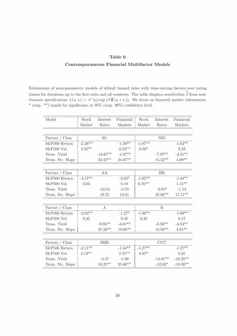
Table 6 presents estimates of sensitivities β for different specifications on the basis of con-
temporaneous financial predictors over rating classes. It enables us to test whether modelsbased solely on stock prices or interest rates or on both (joint model) are sufficient to explainhistorical default intensities.
[INSERT TABLE 6 HERE]
5Indeed, from time series cycle analysis between the GDP and bankruptcy rates, Koopman and Lucas (2004)observe differences in magnitude and lengths. The default cycle being much smoother and persistent than thefinancial market or the business cycles, transitory shocks should not represent the most relevant information.
18
The table presents three multifactor models. For robustness checks, we included a dummyindicating non-US firms. Sensitivities to this non-US indicator were not significant. Likelihoodratio tests identify the joint model as the best one, whereas interest rates alone provide thepoorest fits. This last result confirms findings of Driessen (2005) or Janosi et al. (2002) on creditspreads. Interestingly, stock market volatility is not always significant and its relative impact ondefault is minor with respect to other factors. Such a finding is highly challenging for structuralmodels as the volatility determines the dynamics of equities and as a consequence defaultprobabilities. However BBB and BB classes are significantly affected by market volatility. Thismay be explained by the economic impact (in terms of increased funding cost) of a migrationfrom investment-grade to noninvestment-grade. Some fund managers systematically rule outnoninvestment-grade corporate bonds from their portfolios: at the time of a downgrade fromBBB, numerous funds close their positions, resulting in a jump in credit spread and the costof debt. The market volatility could be a good proxy for that kind of market segmentationbehavior and consequently has to be a key indicator for these classes.
[INSERT FIGURE 1 HERE]
Figure 1 focuses on IG and NIG classes displaying baseline hazard rates for nonparamet-ric (solid line), semi-parametric (solid bold line) and parametric counterparts (dashed lines).Unreported baseline hazards for the ”Interest Rates” model show that our interest rates fac-tors, when considered as a group, are unhelpful determinants of default across rating classes.Conversely, stock market information brings significant explanatory power on the IG class. Ina Merton-like intensity model with additional stochastic liabilities, it could be interpreted asevidence of the level and higher variability of assets being the main determinants of the defaultprobability changes. The baseline hazard is leveled down by 29% on Figure 1(a) thanks tostock indicators. But for each bump in Figures 1(a) and 1(c), deviations from the constant(bold lines) remain significant, implying that the S&P500 return and volatility do not succeedin capturing all shocks of the economy which affect the default riskiness. In particular, for theNIG category, the small difference between α◦NP (u) and α◦ (u) shows that these joint financialcomponents perform poorly on NIG issuers as univariate results suggested.
The analysis of the ”Financial Markets” model evidences how correlated factors can bedamaging. We concentrate on IG and NIG classes on Table 6 and on Figures 1(b) and 1(d).Sensitivities to the long term yield are insignificant. From a statistical standpoint, it can beexplained by the high correlation with the other factors. From an economic standpoint, thelong term yield is less informative on current economic conditions than the market index,and on future growth opportunities than the term structure slope. Figure 1(d) proves thatmisspecified and correlated factors dramatically reduce the explanatory power. The light curve
19
(all financial factors) lies above the nonparametric model, meaning that the model introducesadditional noise in hazard rates instead of improving the fit. The bold line, on the other hand,shows the baseline hazard when the sensitivity to the treasury yield is constrained to be null.For the IG (resp. NIG) category, the other coefficients become –1.53**, 2.64* and 27.12**(resp. 1.67**, 0.62* and 6.29**). Both Figure 1(b) and 1(d) prove in this constrained casethe benefit to extract additional information from the term structure slope. The variations inhazard rates explained by this specification are about 43% for IG and 12% for NIG.
Finally, we observe that a constant hazard either unconditional or conditional on financialinformation does not represent the data correctly. Short term default probabilities are com-pletely overstated by standard hazard models (the dashed line is higher than α◦ (u) up to 2 to4 years) as well as long term default probabilities for NIG. Introducing financial factors leadsto overestimating long term hazard rates on a larger part of the debt life. In an attempt tocapture effects of the 2001 default peak, the model grants too much weight to covariations be-tween the financial markets and defaults, yet still undershoot this peak. Notice that given oursample window, the 2001 recession is responsible to a large extent for the first hump of α◦NP (u)(among NIG observed times-to-default which range between 1 to 5 years approximately onefourth faced the 1991 recession at these horizons while one half faced the 2001 recession).6
5.2. Models Based on Non Financial Information
Table 7 reports multifactor specifications using business and credit information. All factorsenter the various models with the same signs. Unlike Duffie et al. (2007) who worked onbankruptcy rates, we observe that the real GDP and the Personal Income Growth are comple-mentary explanatory variables for our dataset. The impact of the GDP increases as the creditquality decreases whereas that of the PIG decreases. This is in accordance with univariateresults. All factors from the credit cycle are significant. In particular, the impact of the BBBspread is homogenous across rating classes, and so are the effects of the NIG downgrade rate.This homogeneity can indicate the influence of changes in the default risk premium. Higherpremia increase future coupon rates as most of companies issue floating rate bonds, pushingsome firms up to their limit. As one could expect, the IG downgrade rate brings defaultinformation for IG hazard rates. But looking at rating classes, we observe that the effects
6We check this overfitting problem due to the 2001 recession by estimating the ”Stock Market” model on thesub-sample constituted by firms entered in the process after the 03/01/1991. This basically cuts durations higherthan 10 years, and thus the second hump on intensity graphs. On this reduced sample the model delivers highersensitivities of -2.82 on the S&P500 return and of 3.14 on its volatility for IG, -1.99** and 0.88** respectivelyfor NIG. At the same time, it also exhibits a higher overestimation of instantaneous probabilities from the 6 to10 remaining years after the peak.
20
are starker around BBB and BB firms. This factor captures local demand and supply shockswhereas the NIG downgrade rate captures global health of issuers.
[INSERT TABLE 7 HERE]
For each rating class, we report as the ”Non Financial” model the best model using thesefive factors. The model is selected from likelihood ratio tests. Figures 2(a) and 2(c) plotscorresponding baseline hazards for IG and NIG categories. It is striking to observe that theGDP does not add information on the IG likelihood of default whereas the situation reversesfor NIG (actually, substituting the PIG by the GDP do not modify significantly the likelihoodfor the BBB class). As we previously mentioned, this split between the GDP and the PIGover rating classes can be explained by the effect of interest rates and their correlation withthe PIG: Adding the term structure slope makes the PIG insignificant on investment-gradefirms but does not change impacts of the GDP. Our results explain the findings of Duffie etal. (2007) since they do not include interest rates information. It could also reflect that theirsample consists mainly of investment-grade firms.
[INSERT FIGURE 2 HERE]
Figures 1(b) and 2(a) show that IG firms are more closely linked to financial markets than tothe other components of the economy. The semi-parametric baseline hazard is indeed higher forthe ”Non Financial” model than for the ”Financial Markets” model. Conversely, consideringNIG firms, the business cycle and credit specific information have much larger impacts ondefault hazard rates than stock and interest rates information. The ”Non Financial” modelexplains 48% of the variation in NIG hazard rates, and 34% of the changes in IG hazard rates.
5.3. Benefits of Considering All Current Economic Indicators
In traditional structural or intensity-based models market factors are expected to integrateinformation on the business cycle or on credit specific phenomena. However these factorsmay merely supply a noisy signal of the business cycle and may not be the most efficientvehicle of financial information. We have shown above that financial information is of primeimportance for explaining default probability changes of IG firms. Nonfinancial informationis more relevant for NIG firms. We will now test whether financial and nonfinancial variablesare complementary or substitute predictors of the default cycle. The top part of the Table 8presents our best global models, over IG, NIG and BBB to CCC classes.
21
[INSERT TABLE 8 HERE]
Both broad categories of factors (financial and nonfinancial) form part of the most relevantinformation set. However, some individual factors are no longer statistically significant. Thereturn of the S&P500 is not relevant for all classes except the AA (unreported). Both itscorrelations with the business cycle (36% with the GDP) and with the BBB spread (-46%)explain this result. It confirms that the market index is too noisy to provide fully reliableinformation on changes in overall default risk. Because of the significant impact of the termstructure slope, the PIG is also insignificant and does not contribute to the explanatory power ofthe model, according to likelihood ratio test. The GDP, on the other hand, is a key instrument.As before, the IG downgrade ratio has significant impact on the BBB and BB classes. Novariable should be added from LR test outputs.
Figures 2(b) and 2(d) show the baseline hazards for the global models. The IG baseline isstrongly shifted downwards by 62% compared to the previous specification. The NIG baselineis very similar to the baseline of the ”Non-Financial” model, explaining 49% of the variations inhazard rates. These results prove that financial and non financial factors are complementaryand should be included in any model of default probabilities under the historical measure.Nevertheless, we remark that the informational content of stock and interest rates markets onthe default likelihood of NIG issuers is highly limited. For that kind of issuers, it is crucialto rely on business factors. The proportions of explained hazard variations of our models aremuch higher than the reported 25% to 30% by Collin-Dufresne et al. (2001) on credit spreads.This evidence that the new factors are key determinants of the default regime changes even ifthe NIG model is not fully satisfactory. In particular the level of the first hump (Figure 2(d))suggests that the default cycle is longer than the business cycle and that some persistency hasstill to be incorporated.
To verify our observations, we test whether the different models are misspecified or not.Well specified models could indeed be used in risk management and pricing applications. Thereexists no full specification test of semi-parametric hazard models a la Cox (test of the para-metric part could be done), but Fernandes and Grammig (2005) have proposed an asymptoticspecification test of parametric hazard models. We can therefore assume a functional formfor the baseline hazard rate (i.e. specify a conditional distribution of times-to-default) andtest the model using their approach. Figures 1 and 2 show that the conditional exponentialityis strongly misspecified. Other standard distribution of durations are the Weibull, the log-normal and the log-logistic distributions. Full maximum likelihood estimations show that forall baseline hazards across rating classes, similar fits are obtained with the log-logistic and the
22
log-normal distribution. Hereafter, we check misspecification of conditionally log-logistic factormodels. Keeping previous notations, hazard models with log-logistic baseline are defined by:
λ (u, ti) =δp (δu)p−1
1 + (δu)p exp(β′Z (ti, u + ti)
) ∀i, (8)
δ and p being the parameters of the baseline hazard. The asymptotic theory doubtfully appliesto our limited samples. We rather propose a specification test in finite samples, starting fromthe Fernandes and Grammig statistic and using bootstrap:
1. Estimate θ (θ = (δ, p, β)) and α◦NP (u) on the observed durations U = (U1, .., UN ).
2. Compute the statistic Λ(θ)
=∫ (
u∫0
(α
(u; t·, θ
)− α◦NP (u; t·)
)du
)2
dF (u) where F is
the true probability function of the Uis.
3. Draw a new uncensored duration sample D(i) =(D
(i)1 , .., D
(i)N
)from the estimated dis-
tribution f(u; t·, θ
), called a bootstrap sample.
4. Apply a uniform right censoring scheme matching the censoring percentage of the ob-served sample. It creates simulated durations U(i) =
(U
(i)1 , .., U
(i)N
).
5. Estimate θ(i) and α◦(i)NP (u) on the simulated sample U(i), and compute the correspondingstatistic Λ
(θ(i)
).
6. Repeat steps 3 to 5 S times, and obtain the empirical distribution of the statistic Λ(θ(·)
),
called the bootstrap distribution.
7. Reject the null hypothesis of correct specification at significance level 5% if Λ(θ)
islarger than the 95% percentile of the bootstrap distribution.
This type of bootstrap procedures is known to work extremely well in finite samples. Noticethat dates of entry into the risk classes are kept fixed (parametric bootstrap). The bottompart of Table 8 displays pvalues based on 1000 bootstrap samples for the ”Financial Markets”,the ”Non Financial” and the ”Global” models, where non significant sensitivities have beenconstrained to zero. Results confirm previous graphical outputs and likelihood ratio tests.The ”Non Financial” model performs quite well over classes from BBB to CCC and for thebroader NIG category. As expected, in the case of NIG firms and junk issuers, modeling hazardrates by means of financial factors is strongly rejected. Nevertheless, stock and interest ratesinformation is sufficient to capture changes in hazard rates of IG firms. Unreported results
23
corroborate the inability of conditionally exponential models to represent the data at a 99.9%confidence level. We also checked that simple unconditional log-logistic models are rejected.As a consequence, it is necessary both to rely on a complete set of economic factors and totake ageing effects (from the most recent rating review) into account so as to correctly captureand predict hazard rates. When using all sources of information, results are less conclusive.The ”Global” model is indeed rejected at 95% over CCC and IG classes. Correlation betweenthe different factors may be at the origin of these misspecifications.
5.4. Trends and Persistency of Shocks
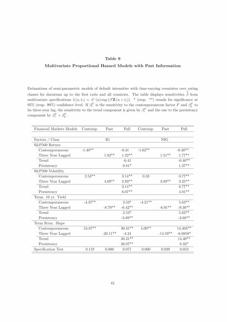
So far, all selected variables have been contemporaneous, but potential lead-lag effects betweenthe economy and the default cycle should also be considered. Looking back at Table 2, wecan argue that lagged variables bring information upon current economic conditions, and somevariables lead the default cycle by an average of three years. In order to address the benefits ofpast information, we concentrate on the ”Financial Markets” model which is the most akin tostructural Merton-type models. We add three-year lagged volatility and stock market return,10-year treasury yield and term structure slope. Estimated parameters
β are provided in Table9 using past information only, and using both contemporaneous and past information.
[INSERT TABLE 9 HERE]
In the complete case, we also report for each factor two additional sensitivities which deliveranother decomposition of the usefulness of information. The ”trend” is the sensitivity whichcan be attributed to the differential between the contemporaneous and the three-year laggedfactor, whereas the ”persistency” is the total sensitivity to the lagged factor. Using pastinformation only, results are in line with univariate analyzes. Past increases in volatility and10-year treasury yield respectively increase and decrease the default likelihood but the effectsare stronger than that of contemporaneous factors. It supports the presence of a significantlag between the financial cycle and the default cycle. The sensitivity to past changes in theterm structure slope becomes negative. We discussed that point for the particular CCC class:three years later, the remaining informational content of past slopes lies in growth anticipation.The positive sign of the sensitivity to the S&P500 return is less obvious. We still advocatefor anticipation of changes in the business cycle which is confirmed by the ”Full” model. Letus consider a concrete situation. Assume that we were at the top of an economic expansionthree years earlier, i.e. the persistency factor is positive. The more the trend factor is negative(the smaller today returns are with respect to past ones), the higher the default likelihood is.Further assume that three years earlier we were at the very beginning of the expansion period.
24
The more the trend factor is positive, the lower the default likelihood is provided that the”growth” or the differential is higher than a given point depending on past conditions (e.g.from Table 9 −(1.37×Z(t−3yr.))
(−0.40) for the NIG case).
[INSERT FIGURE 3 HERE]
From a global perspective, Table 9 shows that both trend and past information are deter-minants of default probabilities. The ”Full” models are not rejected while the ”Past” modelsare. This shows that it is not sufficient to consider the lag between the economy and the defaultcycle. Figures 3(a) and 3(b) confirm the poor explanatory power of past information alone butFigures 3(b) and 3(d) diagnose high explanatory power when it is used with contemporaneousfactors in order to capture economic trends. Explained variations in hazard rates reach 78% forIG and 59% for NIG categories. The improvement is even more substantial than that achievedby additional business and credit indicators for the NIG class.
We can propose two explanations for such findings. First, it may reflect some cyclicalityin equity returns, and an idiosyncrasy of the period we are studying. We have found thathigh current equity returns tend to be associated with low current default rates. If there iscyclicality in equity returns, with a peak-to-trough time of approximately 3 years, it is plausiblethat high returns will be associated with high default rates 3 years on. Nonetheless, we havefound no evidence of such a cyclicality since ”Past” models do not perform in explaininghazard rate variations. An alternative, more likely, explanation would be that in good times(when the equity market is performing well), companies can afford to raise large amounts ofdebt while preserving acceptable levels of leverage. Several years later, this level may becomeunsustainable for some firms, thereby raising the default rate. Table 9 and Figures 3(b) and3(d) do not contradict such a hypothesis. If the stock market has an upward trend, the marketappreciation induces a decrease in hazard rates. If the market depreciates or stagnates, hazardrates increase as some firms start experiencing difficulties.
Summary
In this paper, we study times-to-default in the Standard & Poor’s rated universe using hazardmodels. We rely on a tractable framework that enables us to analyze the behavior of defaultprobabilities with respect to changes in various economic indicators. This is done under thehistorical measure to focus precisely on probabilities without any perturbations due to changesin the default risk premium. The paper concentrates on common default determinants andinvestigates default probabilities, rather than bankruptcy rates as considered in most previous
25
research. Our setting also highlights the distribution of explanatory errors through time. Themodels we propose can be operated to forecast default probabilities at any horizon, and as aconsequence, as inputs to standard credit risk applications.
We examine different economic components which should alter the default cycle and quan-tify their explanatory power: financial market information, the business cycle and endogenousproxies from credit markets and the default cycle. We explore further the sensitivity of de-fault probabilities to past economic conditions and show their persistency as well as impactsof subsequent trends. Specification tests for parametric hazard rate models are also proposedand applied to time-to-default modeling.
Our initial empirical results show that the business cycle and financial market factors offercomparable explanatory powers. Business cycle changes have larger influences on NIG issuerswhereas stock and bond market indicators are key determinants of future default probabilitiesof IG companies. Leverage ratio-targeting and business diversification provide some intuitionfor this phenomenon. We show that selecting a set of factors from each economic components(financial, business, credit) outperforms other specifications in capturing movements in defaultprobabilities.
Results on impacts of the market volatility are challenging for structural models as stockprice volatility is only really significant for the BBB and BB classes which are more stronglyimpacted by supply and demand phenomena. However, a lag between the market and de-fault rates can explain these results as lagged volatility is a significant determinant of defaultprobabilities for all issuers.
26
References
Altman E.I. (1989): Measuring Corporate Bond Mortality and Performance, Journal of Finance44: 909-922
Altman E.I, Rijken H.A. (2004): How Rating Agencies Achieve Rating Stability, Journal ofBanking and Finance 28: 2679-2714
Andersen P., Borgan O. , Gill R., Keiding N. (1997): Statistical Models Based on CountingProcesses, Springer-Verlag, 2nd Edition, New York
Andersen P., Gill R. (1982): Cox’s Regression Model for Counting Processes : A Large SampleStudy, The Annals of Statistics 10:4: 1100-1120
Bangia A., Diebold F.X., Kronimus A., Schagen C., Schuermann T. (2002): Ratings migrationand the business cycle, with application to credit portfolio stress testing, Journal of Bankingand Finance 26: 445-474
Chen S.X. (2000): Probability Density Functions Estimation Using Gamma kernels, Annals ofthe Institute of Statistical Mathematics 52: 471-480
Collin-Dufresne P., Goldstein R.S., Martin S.J. (2001): The Determinants of Credit SpreadChanges, Journal of Finance 66:6: 2177-2207
Couderc F. (2005): Understanding Default Risk Through Nonparametric Intensity Estimation,Swiss Finance Institute (FAME) Research Series 141
Cox D.R. (1972): Regression Models and Life Tables. Royal Statistical Society 2: 187-220
Cremers M., Driessen J., Maenhout P., Weinbaum D. (2006): Explaining the Level of CreditSpreads: Option-Implied Jump Risk Premia in a Firm Value Model, BIS Working Paper191
Driessen J. (2005): Is default event risk priced in corporate bonds?, Review of Financial Studies18: 165-195
Duffee G.R. (1998): The Relation between Treasury Yields and Corporate Bond Yield Spreads,Journal of Finance 53: 2225-2241
Duffee G.R. (1999): Estimating the price of default risk, Review of Financial Studies 12:197-226
Duffie D., Singleton K.J. (2003): Credit Risk - Pricing, Measurement, and Management,Princeton Series in Finance
Duffie D., Saita L., Wang K. (2007): Multi-Period Corporate Default Prediction With Stochas-tic Covariates, Journal of Financial Economics 83: 635665
27
Ericsson J., Renault O. (2006): Liquidity and Credit Risk, Journal of Finance 61: 2219-2250
Fernandes M., Grammig J. (2005): Nonparametric Specification Tests for Conditional DurationModels, Journal of Econometrics 127:1: 35-68
Fledelius P., Lando D., Nielsen J.P. (2004): Non-parametric analysis of rating transition anddefault data, Journal of Investment Management 2: 71-85
Fons J.S. (1991): An Approach to Forecasting Default Rates, Moody’s Special Report
Helwege J., Kleiman P. (1997): Understanding Aggregate Default Rates of High Yield Bonds,Journal of Fixed Income, June
Janosi T., Jarrow R., Yildirim Y. (2002): Estimating expected losses and liquidity discountsimplicit in debt prices, Journal of Risk 5:1
Jonsson J.G., Fridson M. (1996): Forecasting Default Rates on High Yield Bonds, Journal ofFixed Income, June
Kavvathas D. (2000): Estimating Credit Rating Transition Probabilities for Corporate Bonds,University of Chicago
Koopman S.J., Lucas A. (2004): Business and Default Cycles for Credit Risk, Journal ofApplied Econometrics 20:2: 311-323
Koopman S.J., Lucas A., Monteiro A.A. (2008): The Multi-State Latent Factor IntensityModel for Credit Rating Transitions, Journal of Econometrics 142:1:399-424
Loffler G. (2004): An Anatomy of Rating Through the Cycle, Journal of Banking and Finance28: 695-720
Merton R. (1974): On the Pricing of Corporate Debt : the Risk Structure of Interest Rates,Journal of Finance 29: 449-470
Nickell P., Perraudin W., Varotto S. (2000): Stability of ratings transitions. Journal of Bankingand Finance 24: 203-227
Prigent J.-L., Renault O., Scaillet O. (2001): An Empirical Investigation into Credit SpreadIndices, Journal of Risk 3: 27-55
For parametric hazard rate models, the standard estimation procedure relies on the maximumlikelihood technique and works in the following way. Assuming that structural variables dy-namics are independent, the likelihood is separable into two terms, one related to the dynamicsof factors and the other dealing with conditional durations. Therefore, if we are not interestedin factors dynamics, we can ignore this part and focus purely on time-to-default. For a givenfirm i, the likelihood l of observed duration ui can be written conditionally on factor realiza-tions at firm’s ”death or exit” but the whole construction of the risk classes information sethas to be known up to that calendar time:
l (ui) = l1(ui| F Z
ti+ui
)× l2(F Z
ti+ui
)
where l1 is the univariate likelihood of the conditional duration and l2 the likelihood associ-ated with the factor dynamics. From that point, letting L1 and L2 denote the multivariatecounterparts of l1 and l2, the multivariate likelihood function for a sample of n firms observedup to time t = max
i{ti + ui} is defined by
L (u1, .., un) = L1
(u1, .., un| F Z
t
)× L2
(F Zt
)
with
L1
(u1, .., un| F Z
t
)=
n∏
i=1
exp(−
∫ ui
0λ (s, ti) ds
) (I(di>ci) + λ (ui, ti) I(di≤ci)
)(9)
where c1, .., cn (resp. d1, .., dn) are realizations of censoring variables C1, .., Cn (resp. defaultdurations D1, .., Dn).
29
0 5 10 15 200
0.5
1
1.5
2
2.5
3x 10
−5
Haz
ard
Rat
e
Time−to−Default
(a) IG, ”Stock Market” model
0 5 10 15 200
0.5
1
1.5
2
2.5
3x 10
−5
Time−to−Default
Haz
ard
Rat
e
(b) IG, ”Financial Markets” model
0 5 10 15 200.5
1
1.5
2x 10
−4
Haz
ard
Rat
e
Time−to−Default
(c) NIG, ”Stock Market” model
0 5 10 15 200.4
0.6
0.8
1
1.2
1.4
1.6
1.8
2
2.2
2.4x 10
−4
Haz
ard
Rat
e
Time−to−Default
(d) NIG, ”Financial Markets” model
Figure 1
Baseline Hazards of Multifactor Models Relying on Financial Information
Estimated nonparametric baseline hazard rates (α◦NP (u), α◦ (u)) and corresponding meansover investment grades and noninvestment Grades. Thin lines denote the full non-parametric model (α (u, ti) = α◦ (u)) and bold lines show semi-parametric specifications(α (u, ti) = α◦ (u) exp (β′Z (u + ti))) including only significant factors whereas light lines keepall factors. Dashed lines represent averages of baselines - they are not statistically different from theestimated constants exp(γ) of parametric model counterparts (α (u, ti) = exp (γ + β′Z (u + ti))). The”Stock Market” model uses the contemporaneous return and volatility on the S&P500. The ”FinancialMarkets” model includes in addition the US Long Term Yield and Term Structure Slope.
30
0 5 10 15 200
0.5
1
1.5
2
2.5
3x 10
−5
Haz
ard
Rat
e
Time−to−Default
(a) IG, ”Non Financial” model
0 5 10 15 200
0.5
1
1.5
2
2.5
3x 10
−5
Haz
ard
Rat
e
Time−to−Default
(b) IG, ”Best Global” model
0 5 10 15 200.2
0.4
0.6
0.8
1
1.2
1.4
1.6
1.8
2x 10
−4
Time−to−Default
Haz
ard
Rat
e
(c) NIG, ”Non Financial” model
0 5 10 15 200.2
0.4
0.6
0.8
1
1.2
1.4
1.6
1.8
2x 10
−4
Haz
ard
Rat
e
Time−to−Default
(d) NIG, ”Best Global” model
Figure 2
Baseline Hazards of Non Financial and Global Multifactor Models
Estimated nonparametric baseline hazard rates (α◦NP (u), α◦ (u)) and corresponding means over invest-ment grades and noninvestment grades. Thin lines denote the full non-parametric model (α (u, ti) =α◦ (u)) and bold lines show semi-parametric specifications (α (u, ti) = α◦ (u) exp (β′Z (u + ti))).Dashed lines represent averages of baselines - they are not statistically different from the estimatedconstants exp(γ) of parametric model counterparts (α (u, ti) = exp (γ + β′Z (u + ti))). The ”NonFinancial” model uses the BBB Spread, the IG and NIG downgrade rates. In addition, the IG modelrelies on the Personal Income Growth and the NIG model on the Real Gross Domestic ProductGrowth. The ”Best Global” model relies on the S&P500 volatility, the Term Structure Slope, theGDP, the BBB Spread and both IG and NIG downgrade rates.
31
0 5 10 15 200
0.5
1
1.5
2
2.5
3x 10
−5
Haz
ard
Rat
e
Time−to−Default
(a) IG, ”Past Financial Markets” model
0 5 10 15 200
0.5
1
1.5
2
2.5
3x 10
−5
Haz
ard
Rat
e
Time−to−Default
(b) IG, ”Full Financial Markets” model
0 5 10 15 200.5
1
1.5
2x 10
−4
Haz
ard
Rat
e
Time−to−Default
(c) NIG, ”Past Financial Markets” model
0 5 10 15 200.2
0.4
0.6
0.8
1
1.2
1.4
1.6
1.8
2x 10
−4
Haz
ard
Rat
e
Time−to−Default
(d) NIG, ”Full Financial Markets” model
Figure 3
Baseline Hazards of MultiFactor Models with Past Information
Estimated nonparametric baseline hazard rates (α◦NP (u), α◦ (u)) and corresponding means over invest-ment grades and noninvestment grades. Thin lines denote the full non-parametric model (α (u, ti) =α◦ (u)) and bold lines show semi-parametric specifications (α (u, ti) = α◦ (u) exp (β′Z (u + ti))).Dashed lines represent averages of baselines - they are not statistically different from the estimatedconstants exp(γ) of parametric model counterparts (α (u, ti) = exp (γ + β′Z (u + ti))). The ”Past”model uses three-year lagged factors (S&P500 return and volatility, 10 yr. treasury yield and termstructure slope). The ”Full” models add the same comporaneous factors.
32
Table 1
Statistics on Covariates
Basic statistics on retained factors. Figures are given on an annual basis, and in percentages (exceptfor the skewness). All variables but upgrade and downgrade rates are US indicators.
Estimations of log-linear intensities λ (u, ti) on IG and NIG with time-varying covariates over the wholesample up to last days of observation. The table displays sensitivities β from univariate specificationsλ (u, ti) = exp (γ + β′Z (u + ti)) where the default arrival is assumed to be piecewise exponentialconditional on factor realizations. We consider lags from five years backward to two months forward- only main lags are reported. Constants γ are not reported. * (resp. **) stands for significance at95% (resp. 99%) confidence level. For each factor the lag offering the highest likelihood ratio has beenstressed in italics. Other figures display percentage changes in the hazard rate for minus/plus onestandard deviation changes in the factor.
Investment GradesLag S&P500 Return S&P500 Vol. Treas Yield Term Str.Slope
-1M-2.25**
42.69/-29.923.36**
-21.75/27.80-15.98**
56.43/-36.0740.69**
-36.08/56.45
0M-2.72**
53.69/-34.933.80**
-24.22/31.97-15.33**
53.61/-34.9038.44**
-34.48/52.63
1M-2.85**
56.88/-36.263.99**
-25.27/33.81-15.35**
53.70/-34.9433.11**
-30.53/43.94
3M-2.61**
51.04/-33.793.50**
-22.55/29.11-13.90
47.58/-32.2428.29**
-26.74/36.50
1Y-1.96**
36.30/-26.632.59**
-17.23/20.81-11.07**
36.34/-26.65-3.56
3.99/-3.84
3Y1.33**
-18.95/23.393.85**
-24.50/32.45-11.75**
38.96/-28.04-20.84**
25.76/-20.49
Noninvestment GradesLag S&P500 Return S&P500 Vol. Treas Yield Term Str.Slope
-1M-1.89**
34.80/-25.81.81**
-12.38/14.13-10.91**
35.73/-26.3222.54**
-21.96/28.14
0M-1.96**
36.30/-26.632.10**
-14.21/16.57-10.41**
33.84/-25.2819.66**
-19.45/24.14
1M-2.05**
38.25/-27.672.39**
-16.01/19.06-10.44**
33.95/-25.3516.93**
-16.99/20.47
3M-2.01**
37.38/-27.212.47**
-16.50/19.76-10.03**
32.42/-24.4910.98**
-11.38/12.84
1Y-1.02**
17.49/-14.881.99**
-13.52/15.64-7.05**
21.82/-17.91-19.00**
23.24/-18.86
3Y1.66**
-23.07/29.993.60**
-23.11/30.06-12.21**
40.76/-28.96-21.08**
26.10/-20.70
34
Table 3
Sensitivities w.r.t. Business Cycle Information
Estimations of log-linear intensities λ (u, ti) on IG and NIG with time-varying covariates over the wholesample up to last days of observation. The table displays sensitivities β from univariate specificationsλ (u, ti) = exp (γ + β′Z (u + ti)) where the default arrival is assumed to be piecewise exponentialconditional on factor realizations. We consider lags from five years backward to two months forward- only main lags are reported. Constants γ are not reported. * (resp. **) stands for significance at95% (resp. 99%) confidence level. For each factor the lag offering the highest likelihood ratio has beenstressed in italics. Other figures display percentage changes in the hazard rate for minus/plus onestandard deviation changes in the factor.
Investment GradesLag Real GDP Growth Ind. Prod Growth CPI Growth Pers. Inc Growth
-1M-17.47**
39.37/-28.25-48.37**
33.67/-25.19-15.85**
35.14/-26.00-27.13**
86.64/-46.42
0M-19.23**
44.10/-30.61-38.40**
25.91/-20.58-15.08**
33.18/-24.91-26.74**
84.97/-45.94
1M-20.81**
48.50/-32.66-46.55**
32.22/-24.37-12.77*
27.46/-21.54-25.14**
78.29/-43.91
3M-21.91**
51.63/-34.05-57.27**
41.00/-29.08-9.85**
20.58/-17.07-22.16**
66.48/-39.93
1Y-12.62**
27.10/-21.32-47.77**
33.19/-24.92-2.76
5.38/-5.11-9.72**
25.05/-20.03
3Y15.32**
-25.25/33.795.99
-3.53/3.66-16.07**
35.71/-26.31-.40
0.92/-0.92
Noninvestment GradesLag Real GDP Growth Ind. Prod Growth CPI Growth Pers. Inc Growth
-1M-21.44**
50.28/33.46-39.38**
26.65/-21.04-7.87**
16.13/-13.89-19.82**
57.75/-36.61
0M-22.66**
53.81/-34.98-36.20**
24.26/-19.52-5.87**
11.80/-10.55-18.78**
54.02/-35.08
1M-23.01**
54.84/-35.42-50.57**
35.45/-26.17-4.47*
8.86/-8.14-17.26**
48.73/-32.77
3M-22.58**
53.58/-34.89-54.06**
38.31/-27.70-2.02
3.91/-3.77-13.16**
35.35/-26.12
1Y-6.78**
13.75/-12.09-35.55**
23.78/-19.21.53
-1.00/1.01-.45
1.04/-1.03
3Y11.71**
-19.95/24.9213.65**
-7.86/8.53-15.50**
34.25/-25.511.34
-3.03/3.13
35
Table 4
Sensitivities w.r.t. Credit Markets Information
Estimations of log-linear intensities λ (u, ti) on IG and NIG with time-varying covariates over the wholesample up to last days of observation. The table displays sensitivities β from univariate specificationsλ (u, ti) = exp (γ + β′Z (u + ti)) where the default arrival is assumed to be piecewise exponentialconditional on factor realizations. We consider lags from five years backward to two months forward- only main lags are reported. Constants γ are not reported. * (resp. **) stands for significance at95% (resp. 99%) confidence level. For each factor the lag offering the highest likelihood ratio has beenstressed in italics. Other figures display percentage changes in the hazard rate for minus/plus onestandard deviation changes in the factor.
Estimations of log-linear intensities λ (u, ti) with time-varying covariates over the whole sampleup to last days of observation. The table displays sensitivities β from univariate specificationsλ (u, ti) = exp (γ + β′Z (u + ti)) where the default arrival is assumed to be piecewise exponentialconditional on factor realizations. Constants γ are not reported. * (resp. **) stands for significanceat 95% (resp. 99%) confidence level. Other figures display percentage changes in the hazard rate forminus/plus one standard deviation changes in the factor.
Default Factors / Class IG AA A BBB
IG Upgrade Rate-55.70**
18.19/-15.39-6.34
1.92/-1.88-16.69
5.13/-4.88-38.85
12.36/-11.00
NIG Upgrade Rate-18.87**
18.51/-15.62-5.05
4.65/-4.45-7.65
7.13/-6.65-22.78
22.75/-18.53
IG Downgrade Rate72.91**
-39.97/66.5938.52
-23.63/30.9553.03**
-31.01/44.9564.62**
-36.39/57.20
NIG Downgrade Rate23.80**
-26.61/36.2622.43
-25.29/33.8524.38**
-27.16/37.2923.82**
-26.63/36.30
Default Factors / Class NIG BB B CCC
IG Upgrade Rate-68.35**
22.76/-18.54-42.94**
13.75/-12.09-68.57**
22.84/-18.59-70.05**
23.39/-18.95
NIG Upgrade Rate-30.30
31.35/-23.87-28.42
29.14/-22.57-33.66**
35.38/-26.13-41.23**
44.93/-31.00
IG Downgrade Rate50.22**
-29.64/42.1359.40**
-34.02/51.5650.42**
-29.74/42.3234.75**
-21.59/27.54
NIG Downgrade Rate24.91**
-36.48/57.4325.41**
-28.13/39.1426.21**
-28.87/40.5923.99**
-26.79/36.60
37
Table 6
Contemporaneous Financial Multifactor Models
Estimations of semi-parametric models of default hazard rates with time-varying factors over rating
classes for durations up to the first exits and all countries. The table displays sensitivities β from mul-
tivariate specifications λ (u, ti) = λ◦ (u) exp (β′Z (u + ti)). We focus on financial market information.* (resp. **) stands for significance at 95% (resp. 99%) confidence level.
Estimations of semi-parametric models of default hazard rates with time-varying factors overrating classes for durations up to the first exits and all countries. The table displays sensitivitiesβ from multivariate specifications λ (u, ti) = λ◦ (u) exp (β′Z (u + ti)). We focus on business andcredit information. The ”Non Financial” model displays the best model from this set of factors, onthe basis of likelihood ratio tests. * (resp. **) stands for significance at 95% (resp. 99%) confidence level.
Model Business Credit Non Business Credit NonCycle Cycle Financial Cycle Cycle Financial
Global Multivariate Proportional Hazard Models and Specification Tests
Estimations of semi-parametric models of default intensities with time-varying covariates over IG andNIG classes for durations up to the first exits and all countries. The first part of the table displays
sensitivities β from multivariate specifications λ (u, ti) = λ◦ (u) exp (β′Z (u + ti)). * (resp. **) stands
for significance at 95% (resp. 99%) confidence level. The second part presents pvalues of specificationtests on conditionally log-logistic counterparts.