This article was downloaded by: [Aston University] On: 27 January 2014, At: 07:06 Publisher: Routledge Informa Ltd Registered in England and Wales Registered Number: 1072954 Registered office: Mortimer House, 37-41 Mortimer Street, London W1T 3JH, UK International Economic Journal Publication details, including instructions for authors and subscription information: http://www.tandfonline.com/loi/riej20 Business cycle asymmetries in Turkey: an application of Markov-switching autoregressions Huseyin Tastan a & Nuri Yildirim a a Department of Economics , Yildiz Technical University , Istanbul, Turkey Published online: 03 Oct 2008. To cite this article: Huseyin Tastan & Nuri Yildirim (2008) Business cycle asymmetries in Turkey: an application of Markov-switching autoregressions, International Economic Journal, 22:3, 315-333, DOI: 10.1080/10168730802376151 To link to this article: http://dx.doi.org/10.1080/10168730802376151 PLEASE SCROLL DOWN FOR ARTICLE Taylor & Francis makes every effort to ensure the accuracy of all the information (the “Content”) contained in the publications on our platform. However, Taylor & Francis, our agents, and our licensors make no representations or warranties whatsoever as to the accuracy, completeness, or suitability for any purpose of the Content. Any opinions and views expressed in this publication are the opinions and views of the authors, and are not the views of or endorsed by Taylor & Francis. The accuracy of the Content should not be relied upon and should be independently verified with primary sources of information. Taylor and Francis shall not be liable for any losses, actions, claims, proceedings, demands, costs, expenses, damages, and other liabilities whatsoever or howsoever caused arising directly or indirectly in connection with, in relation to or arising out of the use of the Content. This article may be used for research, teaching, and private study purposes. Any substantial or systematic reproduction, redistribution, reselling, loan, sub-licensing, systematic supply, or distribution in any form to anyone is expressly forbidden. Terms & Conditions of access and use can be found at http://www.tandfonline.com/page/terms- and-conditions
Transcript
This article was downloaded by: [Aston University]On: 27 January 2014, At: 07:06Publisher: RoutledgeInforma Ltd Registered in England and Wales Registered Number: 1072954 Registeredoffice: Mortimer House, 37-41 Mortimer Street, London W1T 3JH, UK
International Economic JournalPublication details, including instructions for authors andsubscription information:http://www.tandfonline.com/loi/riej20
Business cycle asymmetries in Turkey:an application of Markov-switchingautoregressionsHuseyin Tastan a & Nuri Yildirim aa Department of Economics , Yildiz Technical University , Istanbul,TurkeyPublished online: 03 Oct 2008.
To cite this article: Huseyin Tastan & Nuri Yildirim (2008) Business cycle asymmetries in Turkey: anapplication of Markov-switching autoregressions, International Economic Journal, 22:3, 315-333,DOI: 10.1080/10168730802376151
To link to this article: http://dx.doi.org/10.1080/10168730802376151
PLEASE SCROLL DOWN FOR ARTICLE
Taylor & Francis makes every effort to ensure the accuracy of all the information (the“Content”) contained in the publications on our platform. However, Taylor & Francis,our agents, and our licensors make no representations or warranties whatsoever as tothe accuracy, completeness, or suitability for any purpose of the Content. Any opinionsand views expressed in this publication are the opinions and views of the authors,and are not the views of or endorsed by Taylor & Francis. The accuracy of the Contentshould not be relied upon and should be independently verified with primary sourcesof information. Taylor and Francis shall not be liable for any losses, actions, claims,proceedings, demands, costs, expenses, damages, and other liabilities whatsoever orhowsoever caused arising directly or indirectly in connection with, in relation to or arisingout of the use of the Content.
This article may be used for research, teaching, and private study purposes. Anysubstantial or systematic reproduction, redistribution, reselling, loan, sub-licensing,systematic supply, or distribution in any form to anyone is expressly forbidden. Terms &Conditions of access and use can be found at http://www.tandfonline.com/page/terms-and-conditions
International Economic JournalVol. 22, No. 3, September 2008, 315–333
Business cycle asymmetries in Turkey:an application of Markov-switching
autoregressionsHuseyin Tastan* and Nuri Yildirim
Department of Economics, Yildiz Technical University, Istanbul, Turkey
This paper examines business cycle characteristics of the Turkish economy in the liberaliza-tion (post-1980) period using a Markov-switching Autoregressive (MSAR) model framework.The importance of the model selection process is emphasized in an extensive search for theappropriate MS model. The business cycle properties are found to be very sensitive to the statedimension, the choice of the MS model (classified according to regime-dependent parameters)and the autoregressive lag order. The chosen two-regime MS model suggests four recession-ary and five expansionary phases in the post-1980 period. Business cycle phases are found tobe asymmetric with the probability of switching from a recession to expansion exceeding theprobability of switching from expansion to recession. The paper also provides evidence on theusefulness of a non-linear model as compared with a linear alternative in the context of busi-ness cycle research in an emerging economy using various parametric and non-parametrictests. Non-linear and linear models are compared and evaluated using kernel density andconditional expectation estimates by simulating data from respective models.
Keywords: Markov switching AR model; business cycle; asymmetry tests; emergingeconomy; Turkey
JEL Codes: E32; E37; C22
1. Introduction
Economists have long been interested in cyclical properties of macroeconomic variablessuch as gross domestic product, unemployment rate, inflation rate etc. An importantcharacteristic of business cycles is the cyclical asymmetry. Sichel (1993) defines an asym-metric business cycle as the one ‘in which some phase of the cycle is different from themirror image of the opposite phase; for example contractions might be steeper, onaverage, than expansions’ (Sichel 1993, 224).1 If the economy behaves differently over
the phases of business cycles then the policy conclusions from the linear time seriesmodels will potentially be misleading (Hess and Iwata 1997). To ascertain propertiesof business cycles empirically, one needs to determine the dates of turning points forrecessions and expansions. Once turning points are determined one can analyze busi-ness cycles and/or apply asymmetry tests. The methods used to identify business cycleturning points can be classified as parametric and non-parametric (Harding and Pagan2002). In the parametric approach, a statistical model for the series is specified and usedto identify turning points (e.g. Neftci 1982, and the Markov Switching autoregressivemodel of Hamilton 1989). By contrast, non-parametric methods do not require one tofit a statistical model. A leading example of this approach is the NBER dating proce-dure, which is based on ad hoc procedures and the concept of the reference cycle, andits formal algorithm was developed by Bry and Boschan (1971).
Since Hamilton’s (1989) analysis of US business cycles using the regime-switching ARmodel, non-linear parametric methods have become the leading approach for datingand classifying business cycles (Krolzig 2001b). Other competing non-linear parametricmodels include Threshold Autoregression (TAR), Smooth Transition Autoregression(STAR) models and their variants (e.g. LSTAR and ESTAR). In this study, we focus onMSAR models instead of STAR-type models primarily because the regime-switchingis sudden and non-smooth. An attractive feature of MS models is that they provide aflexible framework in which aggregate level of economic activity has a certain proba-bility of switching among a number of states. In a two-regime framework, the modelprovides estimates of conditional and smoothed probabilities of switching betweenrecession and expansion states attached to each observation.
MS models have been extensively used in the empirical literature on business cycles.A significant effort has been devoted to the study of business cycle phenomena in devel-oped countries. For example, Lam (2004) provided evidence on duration dependence ofUS business cycles. Using a multivariate framework, Krolzig (2001a) argued that largepermanent shifts in the long-run growth rate of real GDP in developed countries suchas the US, Japan and Europe cannot be captured by two-regime Markov-switchingmodels; instead, a three-regime model is needed. Similarly, Artis et al. (2004) andKrolzig (2001b) applied MS-VAR methods to identify business cycle turning pointsfor the Euro-Zone and found strong evidence for the existence of a common businesscycle. Taylor et al. (2005) failed to find a significant autoregressive structure (or cyclicalbehavior) in the growth rate of Australian GDP in a Bayesian MS estimation and modelselection framework. On the other hand, the number of studies focusing on businesscycle characteristics in an MS framework in developing countries is rather limited.Notable exceptions include the study of South African business cycles by Moolman(2004) who found that the MS model performs better than linear and logit model alter-natives. Girardin (2005) analyzed business cycle features of 10 East Asian countriesusing three-regime MSAR models. Krutz (2005) estimated a three-regime MS model toMexico to identify business cycle turning points.2
The purpose of this paper is to contribute to the empirical literature on business cycleanalysis in developing countries by examining basic characteristics of business cyclesin Turkish economy. Turkey being a member of the OECD since 1961 is an importantemerging market, entering among the largest 20 economies in the world with a GNPover US$400 billion. Moreover, Turkey has moved forward a long way to become anopen liberal economy through comprehensive structural reforms realized during thelast two decades. Its foreign trade reached 56% of GNP in 2006. The absence of businesscycle studies on the Turkish economy is another motivation for this paper, which wehope might lead to further research on the subject. For the purposes of this paper,
Dow
nloa
ded
by [
Ast
on U
nive
rsity
] at
07:
06 2
7 Ja
nuar
y 20
14
International Economic Journal 317
an MS model of the growth rate of industrial production is estimated and business cycleturning points and phases are identified based on the smoothed regime probabilities.The adequacy of non-linear MS models, in an emerging economy is further investigatedusing parametric and non-parametric encompassing tests suggested by Breunig et al.(2003) and several forecast performance measures.
The paper is organized as follows. Section two briefly summarizes the MS-AR model-ing technique. Section three discusses the data and the problem of choosing appropriateMS formulation. The problems of determining the state dimension, the autoregressivelag order and the form of the model (regime-dependent intercepts versus means andregime-dependent variances versus homoskedasticity) are investigated systematically.This is shown to be useful since the exact dates of turning points are extremely sensi-tive to model components. Section four presents empirical results from the chosen MSmodel and provides parametric and non-parametric encompassing tests and forecastperformance. Section five gives concluding remarks.
2. Markov-switching AR models
Hamilton (1989) used an MS formulation in which only the mean of the process changesaccording to the unobserved state. By adding regime-dependent variance this modelcan be written as:
where st ∈ {1, 2, . . . , n} is a hidden Markov state and εt is IIDN(0,1). The hidden statefollows an n-regime ergodic discrete-time discrete-state Markov process with n × ntransition matrix P. Each entry of the transition matrix represents the probability ofmoving from one-regime to another:
pij = Pr(st = j|st−1 = i),n∑
j=1
pij = 1, ∀i, j ∈ {1, 2, . . . , n}
For example, for a two-state business cycle model of the growth rate of real GDP(or some other measure of economic activity) where st = {1, 2} if the economy is inrecession and expansion respectively, the transition matrix will be
P =[
p11 p12p21 p22
]
where each entry represents conditional probabilities of moving from one state toanother:
p11 = Pr[Recession in time t |Recession in time (t − 1)]p12 = Pr[Recession in time t |Expansion in time (t − 1)]p22 = Pr[Expansion in time t |Expansion in time (t − 1)]p21 = Pr[Expansion in time t |Recession in time (t − 1)]
The model above is commonly known as an MSMH(n)-AR(k) model – a shorthanddue to Krolzig (1997). This model admits a one time change in mean when the process
Dow
nloa
ded
by [
Ast
on U
nive
rsity
] at
07:
06 2
7 Ja
nuar
y 20
14
318 H. Tastan and N. Yildirim
switches from one-regime to another. The model can easily be reformulated to allowfor changes in intercepts if the process is most likely to achieve the new mean levelsmoothly rather than a one time jump.
where cst is the state-dependent intercept term. MSAR models can be classifiedaccording to regime-dependent parameters (Krolzig 1997):
• MSM: Markov-switching means,• MSMA: Markov-switching means and AR parameters,• MSMAH: Markov-switching means, AR parameters and variances,• MSI: Markov-switching intercepts,• MSIH: Markov-switching intercepts and variances,• MSIAH: Markov-switching intercepts, AR parameters and variances.
Details of the estimation algorithms for the class of MS models are well-known andcan be found in Krolzig (1997) and Hamilton (1989, 1994).
3. Data and MS model selection
Our data set consists of a seasonally unadjusted monthly industrial production indexcovering the period 1985:1–2005:9 with base year 1995 denoted IPt. We first obtainedannual growth rates using,
yt = IPt − IPt−12
IPt−12
This eliminates most of the seasonal effects in the series. In addition, in order toremove the effects of religious holidays on yt we have run a simple regression of yt ona constant and a dummy variable for religious holidays.3 We used the residuals fromthis regression plus the estimated constant term in our analysis. The data and its basicproperties are plotted in Figure 1. The mean and median growth rates are 0.0528 and0.0531, respectively. The empirical density estimate indicates that yt is slightly skewedto the left with skewness statistic −0.2756. The plots of ACF, PACF, spectral density andperiodogram indicate a persistent autoregressive structure with exponentially decayingACF and partial autocorrelations cutting off at lag two. Standard unit root tests (notreported but available upon request) indicate that yt is stationary.
To see if the series can alternatively be modeled using STAR-type models, we followedTerasvirta’s (1994) specification strategy. Test results4 indicate that an LSTAR(p) modelis preferable to linear and ESTAR models. Using the AIC, the estimated model is afourth-order LSTAR model:
where GLSTAR is the logistic transition function, which is estimated as follows:
GLSTAR = (1 + exp(−8213(yt−3 + 0.0077)/σy))−1
The speed of adjustment parameter is estimated as 8213, indicating that the transitionbetween regimes is very sharp.5 Thus, MSAR models that allow for sudden regime
Dow
nloa
ded
by [
Ast
on U
nive
rsity
] at
07:
06 2
7 Ja
nuar
y 20
14
International Economic Journal 319
Figure 1. Annual growth rate of industrial production.
changes are more appropriate in capturing the behavior of Turkish business cyclesthan smooth transition autoregressive models.
In empirical applications of MSAR models, one has to decide, (i) the number ofregimes, (ii) model specification (changing intercepts versus changing means, regimedependent AR dynamics and heteroskedasticity) and (iii) lag order of the AR terms(not necessarily in this order). In practice, the state dimension of an MS model isgenerally determined, either informally by visual inspection of the data or by statisti-cally sound procedures such as Likelihood Ratio tests (e.g. Hansen 1992 and Garcia1998) and/or data-dependent model selection criteria (Psaradakis and Spagnolo 2003).However, there are several problems with these approaches: the LR tests do not satisfythe standard regularity conditions under the null hypothesis since some parametersare not identified. Determining the number of regimes based on complexity-penalizedlikelihood criteria such as the Akaike Information Criterion (AIC), the Hannan-QuinInformation Criterion (HQIC) and the Schwarz’ Bayesian Information Criterion (SIC)as suggested by Psaradakis and Spagnolo (2003) is also problematic because one hasto know for certain the AR lag order. In fact, in practice, econometricians have tochoose the state dimension and the AR lag order (and other parameters), as well asthe MS model specification simultaneously. Including too many regimes where they arenon-existent would result in spurious regressions and reduced accuracy of parameterestimates and precision of forecasts. Smith et al. (2006) proposed a new informationcriterion that is based on an explicit approximation to the Kullback–Leibler divergencefor the simultaneous selection of the number of states and variables in a class of MSmodels, including MSAR models. To avoid the problems of over and under-fitting thestate dimension as well as model misspecification, we will employ a combination of
Dow
nloa
ded
by [
Ast
on U
nive
rsity
] at
07:
06 2
7 Ja
nuar
y 20
14
320 H. Tastan and N. Yildirim
these procedures. The quality of regime classification produced by alternative modelswill especially be emphasized and used to choose the final model.
Zhang and Stine (2001) have shown that the autocovariance structure of the MSmodels can be represented by an ARMA(p, q) model. The orders of the ARMA processp and q are shown to be less than the state dimension for the MS models with changingmeans and variance. For example, a two-state Markov switching regime model hasan ARMA(1, 1) representation. The practical implication is that the autocovariancestructure of the data can be used to set a lower bound on the number of regimes p, q < n.The autocovariance structure of our data set can well be represented by an ARMA(1, 2)model (based on ARMA(p, q) model specification search, see also ACF and PACF inFigure 1). Hence, the state dimension can be two or more. Since our sample is not largeenough to identify models with four or more regimes, our specification search will belimited to two- and three-regime models.
Our experimentation with different numbers of regimes, AR lag orders and modelspecifications (see the previous section on MS model formulations) revealed thatsome MS models have difficulty in converging to the global maximum.6 For exam-ple MSIAH(n)-AR(k) and MSMA(n)/MSM(n)–AR(k) specifications have generallyfailed to converge or converged to a local maxima with unstable parameter estimatesand standard errors. Additionally, some three-regime models picked single observa-tions in the data set and identified them as distinct regimes producing spurious statesand cycle dating. Hence, we excluded the models with regime dependent AR parame-ters and changing means from our search for the best MS model. We have adopted thefollowing strategy: first, for a given number of regimes, we estimated MSI(n)-AR(k)and MSIH(n)-AR(k) models for n = 1, 2, 3, and k = 0, 1, . . . , 12. This gives us a totalof 51 models (excluding the single-state linear models). Then we have applied severalmodel selection criteria to choose the AR lag length k for each MSI(n) and MSIH(n)models. We also compared information criteria to choose the number of regimes byfixing the AR lag order. In addition to data-based model selection criteria we have ana-lyzed standardized residuals, the general fit of the model, cycle dating and the qualityof regime classification to guide us through the model selection process.
Figure 2 shows model selection criteria for a given number of regimes n = 2, 3. Outof 13 possible MSI(2) models the HQIC and AIC have chosen 5 and 12, respectively,as the AR lag order whereas the SIC has chosen k = 2. This is not surprising because,as shown by Kapetanios (2001) in the context of Markov-switching AR models, theAIC tends to select larger/more complex models whereas the SIC tends to select moreparsimonious models. Kapetanios (2001) has also shown that, when the number ofregimes is known and fixed, the HQIC and SIC perform better than the AIC in selectingthe correct AR lag order.7 For the MSIH(2)-AR(k) case, the SIC chooses the smallestmodel k = 2, whereas the AIC and HQIC choose k = 10. The lower panels of Figure 2display the information criteria when the true model is assumed to have a three-regimeinstead of two-regime hidden structure. The SIC, HQIC and AIC choose 0, 4 and 12lags, when the variance does not change, respectively. When the variance is allowed tochange across regimes all three information criteria choose the lag order as seven.
Psaradakis and Spagnolo (2003) have shown that data-dependent model selectioncriteria, such as the SIC, HQIC and AIC, can be used to identify the state dimension ofan MS model for known AR lag order if the regime structure is persistent and parameterchanges are not too small across regimes. Their results indicate that the SIC, HQICand AIC all tend to underestimate (more or less) the correct state dimension. We haveplotted three information criteria in Figure 3 to see their behavior in an MSI(n) contextfor a given AR lag order. For example, if the true model was an MSI(n)-AR(k = 1),
Dow
nloa
ded
by [
Ast
on U
nive
rsity
] at
07:
06 2
7 Ja
nuar
y 20
14
International Economic Journal 321
Figure 2. Model selection criteria, n fixed.Note: Minimum values are shown with an asterisk.
the SIC and HQIC would choose n = 2 whereas the AIC would choose n = 3. Whenk = 2, the two-regime model was chosen by the AIC while the single-state is selectedby both the SIC and HQIC. In general, the AIC selects larger state dimension than theSIC and HQIC.
Notice that one needs to know either the number of states to select the AR lag lengthor the AR lag order to select the number of states using the conventional informationcriteria. To overcome this Smith et al. (2006) proposed Markov Switching Criterion(MSC) for the simultaneous selection of the number of states and variables. Using theirnotation,
MSC = −2 log(f (Y, θ )) +N∑
i=1
Ti(Ti + λiK)
δiTi − λiK − 2(3)
where log(f (Y, θ )) is the maximized loglikelihood value, Ti is the sum of the smoothedprobabilities of the ith state over the sample, K is the number of variables and N is thenumber of regimes. They report that choosing δi = 1 and λi = N perform well in theircontrolled experiments. Applying this criterion to our data set we would choose theMSIH(3)-AR(3) model. Using the AIC, SIC and HQIC over all 64 candidate modelswe would choose the MSIH(3)-AR(7) model.8
Dow
nloa
ded
by [
Ast
on U
nive
rsity
] at
07:
06 2
7 Ja
nuar
y 20
14
322 H. Tastan and N. Yildirim
Figure 3. Model selection criteria, k fixed.Notes: All information criteria are from MSI(2)-AR(k) model where k = 1, 2, . . . , 12 (read left to right,e.g. upper left panel is from MSI(2)-AR(1), upper right panel is from MSI(2)-AR(2), etc.). Minimum valuesare shown with asterisk.
It seems that a three-regime model is chosen by the information criteria approach:one recession state (with negative growth) and two expansion states (with medium andhigh growth rates). However, do three-regime models classify business cycles correctly?In other words, should we divide the expansion state into two periods of medium andhigh growth? To assess the properties of regime classification by our candidate modelswe attempted to use the Regime Classification Measure (RCM) developed by Ang andBekaert (2002):
RCM = 100n2 1T
T∑t=1
( n∏i=1
pi,t
)(4)
where T is the sample size, n is the number of regimes, and pi,t is the smoothedprobabilities using the sample information. If the regimes are classified sharply thenthis measure will be close to zero since one of the smoothed probabilities will be close tozero. However, although this measure provides some information in two-regime modelswhere RCM = 400T−1 ∑T
t=1 pt(1 − pt), it may not be useful in models where the state
Dow
nloa
ded
by [
Ast
on U
nive
rsity
] at
07:
06 2
7 Ja
nuar
y 20
14
International Economic Journal 323
dimension is larger than two. The reason is that a three-regime model, for example,may have difficulty in classifying any two regimes out of three while one of them isclassified correctly. Consider the case where the smoothed probability vector at time tis pt = (0.002, 0.498, 0.5). The RCM would give a number close to zero although themodel is not successful in classifying the state of the variable in time t into a medium orhigh growth state. The common practice in the literature for classifying regimes is touse a kind of threshold smoothed probability such as p = 0.5 as suggested by Hamilton(1989). In an ideal MS model, the smoothed probabilities should be close to one orzero. To incorporate this notion we use the following modified regime classificationmeasure:
MRCM = 1T
T∑t=1
n∑i=1
I(pi,t > p) (5)
where I(pi,t > p) is an indicator function taking the value one if pi,t > p and zero oth-erwise. If the regimes are classified sharply using the threshold probability then thismeasure will equal one. The degree of regime classification sharpness will increase ifone uses p > 0.5. Table 1 shows the MRCMs for our candidate models. All smoothedprobabilities are greater than 0.51 in the MSIH(2)-AR(4) model. However, one obser-vation cannot be classified using 0.51 in the MSI(2)-AR(4) model. 99.11% of smoothedprobabilities are greater than 0.51 in both the three-regime MSI and MSIH models.As we use a tighter threshold value for the smoothed probabilities, MRCM steadilydeclines as would be expected. 89.33% and 87.56% of observations can be classifiedinto one of the regimes when p = 0.91 in two-regime MSI and MSIH models, respec-tively. However, only 60.44% and 46.67% of the data points can be classified into one ofthe regimes in three-regime MSIH and MSI models, respectively. We also note that theregime classification properties are very sensitive to the number of regimes and whetherthe model includes regime-dependent variances. Additionally, the three-regime modelstend to classify single observations into medium growth regimes with probabilitieshovering around 0.50–0.60. For example, in the MSIH(3)-AR(3) model, single obser-vations 1990:7, 1992:10 and 1995:2 are classified into a medium growth regime withsmoothed probabilities (0.5686, 0.5989, 0.5376), respectively. Also, the mean durationsof regimes in the three-regime models are extremely short, compared with two-regimemodels. For example, in the MSIH(3)-AR(3) model, the mean duration of the mediumgrowth regime is only 2.2 months which makes it difficult to classify it as a distinctregime. Moreover, the two-regime models describe the switching regime properties ofour data more adequately than three-regime models. We will report empirical resultsfrom a two-regime model in the following.
Table 2 presents parameter estimates from a MSIH(2)-AR(4) model, which includesa switching intercept and variance using the data from 1986:6–2005:9.9 The interceptestimate is −0.0419 in recessions and 0.0605 in expansions with highly significantt-values. There is strong evidence to support the view that the intercept terms aresignificantly different in low-growth and high-growth states. The AR parameters arealso found to be significant except for lag three. The standard error is 0.041 in recessionsand 0.0563 in expansions. The null hypothesis that the two variances are the same inboth regimes is rejected at 5% significance level. The expansion regime is slightlymore volatile than the recession regime. As indicated in Table 2, the likelihood ratiotest statistic for the null hypothesis of linearity against the MS model is calculatedas 20.0662. The LR linearity test statistic has a non-standard distribution under thenull hypothesis and cannot be compared to the usual chi-squared distribution. Theasymptotic distribution of the LR statistic depends on the AR coefficients. Garcia(1998) has shown that the 5% critical value for the LR statistic ranges between 8.48and 8.74. This suggests that there is evidence against the linearity in our data. Figure 4displays the ACF, QQ plot against the normal distribution, density and spectral densityof the standardized residuals. We report two portmanteau tests on the standardizedresiduals, BDS independence test and Ljung–Box autocorrelation test. The BDS teststatistic10 indicates that the null hypothesis of independence cannot be rejected atconventional significance levels. The null hypothesis of no autocorrelation cannot berejected using the LB-Q statistics up to lag orders of 8 and 12. The normality ofstandardized residuals cannot be rejected at 5% significance level.
Figure 5 presents filtered and smoothed probabilities of low-growth state. The prop-erties of the transition matrix and cycle dating are presented in Table 3. The probabilityof a recession in time t conditional on the economy being in recession in time t-1 isestimated as about 90% with ergodic probability 20.11%. The estimated conditionaland ergodic probabilities of an expansion are 97.36% and 79.89%, respectively.
Table 2. Estimation results from Markov-switching and linear AR models.
Notes: p-values are shown in brackets. LB-Q(p) is the Ljung-Box autocorrelation test at lag p.
Dow
nloa
ded
by [
Ast
on U
nive
rsity
] at
07:
06 2
7 Ja
nuar
y 20
14
International Economic Journal 325
Figure 4. Properties of standardized residuals.
Figure 5. Smoothed and filtered probabilities of Turkish business cycles.
The Turkish business cycle dates are also presented in Table 3 using common practicein the MS literature, i.e. classifying the observation at time t into recession (expansion)if the respective smoothed probability is higher than 0.5. The regimes are all classifiedsharply with smoothed probabilities greater than 90%, except for the first recessionperiod in the sample (1988:9–1989:4 with smoothed probability 88%). Although thereare no official business cycle dates for the Turkish economy with which the resultscan be compared, the cycle dating resulting from the MS model closely matches crises
Dow
nloa
ded
by [
Ast
on U
nive
rsity
] at
07:
06 2
7 Ja
nuar
y 20
14
326 H. Tastan and N. Yildirim
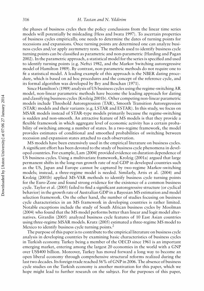
Table 3. Transition probabilities and cycle dating.
Transition matrixrecession Expansion Ergodic probabilities Duration # of obs.
Notes: Based on the estimates from MSIH(2)-AR(4) model. Duration is measured in months.
and downswing periods. The duration of recessions is about 10 months while theduration of expansions is about 38 months (about 3.16 years). These estimates reflectthat recessions are relatively short-lived as compared with other developing economies.Rand and Tarp (2002) found that mean durations of recessions and expansions in aselection of 15 developing countries11 are 5.2 and 4.8 quarters, respectively. Further,the duration of expansion is larger than the average in EU enlargement countries,whereas the duration of recession is shorter (based on Camacho and Perez-Quiros’2006, estimates of expansion and recessions: 26 and 17 months, respectively).
To address the issue of business cycle asymmetry we applied the steepness-deepness-sharpness (SDS) tests developed by Clements and Krolzig (2003). Typically, we say thatthere exists business cycle asymmetry if macroeconomic variables behave differentlyover the phases of the business cycle. Sichel (1993) distinguishes two types of asymme-tries: when contractions are steeper than expansions we have the steepness asymmetryand when troughs are deeper than peaks we have the deepness asymmetry. The sharp-ness or turning point (TP) asymmetry (McQueen and Thorley 1993) occurs if troughsare sharp and peaks are more rounded (Clements and Krolzig 2003). The process yt issaid to be ‘non-deep’ if the skewness is zero (Clements and Krolzig 2003; Sichel 1993):12
E[(yt − μ)3] = 0
where μ = E(yt). The deepness of contractions will show up as negative skewness. Theprocess yt is ‘non-steep’ if the first differenced series has zero skewness:
E[�y3t ] = 0
If contractions are steeper than expansions, �yt will have negative skewness. Thenon-sharpness asymmetry implies that the transition probabilities to and from theouter regimes are the same. Because we have two regimes in our MS model, the non-sharpness condition reduces to p12 = p21. In fact, Clements and Krolzig (2003) haveshown that in the case of two regimes, non-deepness can be tested using H0 : p12 = p21.Hence, non-sharpness implies non-deepness and two-regime MS models are alwaysnon-steep. The results from parametric asymmetry tests of Clements and Krolzig (2003)are shown in Table 4. The non-sharpness test statistic is calculated as 5.0893 withp-value 0.0241. Evidently, the null hypothesis of identical switching probabilities can berejected at 5% significance level. The conditional probability of moving from recession
Dow
nloa
ded
by [
Ast
on U
nive
rsity
] at
07:
06 2
7 Ja
nuar
y 20
14
International Economic Journal 327
Table 4. Tests for business cycle asymmetries from MSIH(2)-AR(4) model.
to expansion (0.1051) is statistically larger than that of moving from expansion torecession (0.0264). The non-deepness test (symmetry) also indicates that recessions aredeeper than expansions.
4.1. Do MS models capture non-linearities in Turkish business cycles?
In this subsection we provide some evidence on how well MS model captures certaincharacteristics of data using parametric and non-parametric methods. The success orfailure of MS model as compared to a simple linear AR model will be investigated bycomparing non-parametric density estimates and parametric encompassing tests.
Recently, Breunig et al. (2003) suggested a set of formal tests and informal compar-ison procedures to assess the success of non-linear models. The formal encompassingtests are simply based on the idea that if the MS models (or any non-linear model)provide a good description of the data then the population characteristics of the modelshould match the observed sample characteristics of the data as closely as possible.Let θ be the maximum likelihood parameter estimates from the MS model and let μbe the mean of some function of data, say m(yt). For example, when m(yt) = yt wehave the sample mean. In addition let yt(θ) be the data set based on a long simulationof the MS model using the ML estimates and let μ(θ ) be the mean associated withm(yt(θ)) using simulated series. Then, the null and alternative hypothesis are given by(Breunig and Stegman 2005):
H0 : μ = μ(θ0)
H1 : μ �= μ(θ0)
where θ0 is the true value of the parameter vector under the null hypothesis that theMS model is correct. In a moment-based test, the (pseudo)-population mean of thefunction m(yt) should match its sample counterpart as closely as possible. Breunig etal. (2003) suggested a Hausman-type test, which is formed as:
τ = (μ − μ(θ ))T[var(μ − μ(θ ))]−1(μ − μ(θ ))
Since it is relatively difficult to get an estimate of var(μ(θ )), Breunig et al. (2003)suggested using var(μ) inside the bracket producing a conservative test.
We simulated 100,000 data points using the ML estimates from both the MSIH(2)-AR(4) model and linear AR(4) (see Table 2). The parametric encompassing test isconstructed for the following functions of the data: mean, variance, and third andfourth moments. Additionally, since the MS models are designed to capture non-linearities in the data, we considered the following quadrant-based encompassingmeasures: the probability of an expansion after a contraction in the previous period, theprobability of an expansion after an expansion in the previous period, the probabilityof an expansion after a contraction in three-periods before and the probability of an
Dow
nloa
ded
by [
Ast
on U
nive
rsity
] at
07:
06 2
7 Ja
nuar
y 20
14
328 H. Tastan and N. Yildirim
expansion after an expansion in three-periods before. These are constructed, respec-tively, for both the sample points and simulated data from the MS and AR models asfollows:
q1 = 1T
∑[I(yt−1 < 0 ∩ yt > 0)]
q2 = 1T
∑[I(yt−1 > 0 ∩ yt > 0)]
q3 = 1T
∑[I(yt−3 < 0 ∩ yt > 0)]
q4 = 1T
∑[I(yt−3 > 0 ∩ yt > 0)]
where I is the indicator function, which takes the value one when the event in the squarebrackets is true and zero otherwise. var(μ) is calculated using the Newey and West(1987) HACC estimator with truncation lag set to nine.13 The test results along withthe measures calculated from the data and non-linear and linear models are displayedin Table 5. The tests are distributed as standard normal under the null hypothesisand the rejection implies that the model does not capture a particular feature of thedata. Both MS and AR models capture the mean and variance of the data well. TheMS model is superior in reproducing the third and fourth moments of the data ascompared with the AR model but is not sufficient to statistically reject the AR model.However, quadrant tests indicate that the MS model is more successful in capturing thenon-linearity apparent in the business cycle data than the AR model. The test statisticsbased on q1 and q3 from the AR model are found as −2.48 and −1.81, which aresignificant at 5% and 10% levels, respectively.
It seems that the basic contribution of the MS model is its ability to capture the prob-ability of an expansion in the current period when there is a recession in the previousperiods. Breunig and Pagan (2004) suggested using non-parametric comparison meth-ods based on kernel density estimates of the data and alternative methods. To comparethe MS and AR models, the kernel density estimates using the same 100,000 simulateddata points are plotted in Figure 6 along with the data. We have used a Gaussian kernelwith bandwidth selected using bw = 1.0592σn−0.2. The peak of the MS model densityestimate is slightly dislocated to the right of the data density while the AR model is
Notes: The test statistic,τ , has a standard normal distribution. ∗∗ and ∗ denote significance at 5% and 10% α-levels,respectively.
Dow
nloa
ded
by [
Ast
on U
nive
rsity
] at
07:
06 2
7 Ja
nuar
y 20
14
International Economic Journal 329
Figure 6. Non-parametric kernel density estimates from the sample, MS model and AR model.
to the left. The MS model seems to be more successful in capturing the skewness andkurtosis apparent in the data. To statistically compare the two model densities to thedata density we calculated the Kolmogorov–Smirnov (KS) test statistics. The KS testsare calculated as 0.0513 and 0.0469 for the MS and AR models with p-values 0.5542and 0.6685, respectively. Evidently, the null hypothesis of identical empirical densitiescannot be rejected for both the MS and AR models.
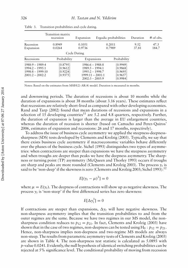
Figure 7 plots non-parametric conditional expectation of yt given yt−1. The condi-tional expectation for the MS model was found using non-parametric kernel regressionas suggested by Breunig and Pagan (2004):
E(yt|yt−1 = z; θ .) =∑T
s=2 ysK((ys−1 − z)/h)∑Ts=2 K((ys−1 − z)/h)
where θ is the ML estimates from the MS model, K(.) is a kernel function, z is aset of chosen values for the conditioning variable and h is the bandwidth. Also, theconditional mean of yt for the linear model is not calculated by simulation but by usingthe theoretical conditional expectations at the AR(4) parameter estimates. Figure 7indicates that there exist non-linearities that cannot be captured by the linear model.The MS model suggests that the expected growth rate for the next period conditionalon the current period starts to increase at lagged growth rates greater than −5%(approximately). The expected (annual) growth rate of Turkish industrial productionin the next period will be higher when the growth rate in the current period is around−5% and 10%. The lagged growth rates higher than 10% are associated with relatively
Dow
nloa
ded
by [
Ast
on U
nive
rsity
] at
07:
06 2
7 Ja
nuar
y 20
14
330 H. Tastan and N. Yildirim
Figure 7. Conditional expectations.
lower expected growth rates in the current period. Since there is a significant differencein conditional means from the MS and AR models, we may expect that using the MSmodel for forecasting would be more beneficial.
4.2. Forecast performance
In this subsection we compare linear and non-linear models in terms of their out-of-sample forecast performance. To do this we followed a recursive estimation scheme inwhich the sample is divided into two periods, the estimation period covering 1986:2–2000:6 and the forecast period covering 2000:7–2005:9. The forecast period is chosensuch that it covers both recession and expansion phases. First, both MS and AR modelsare estimated using the estimation period and one-period-ahead forecasts are obtained.Then, the forecast period’s observation is added to the sample and the next period’s
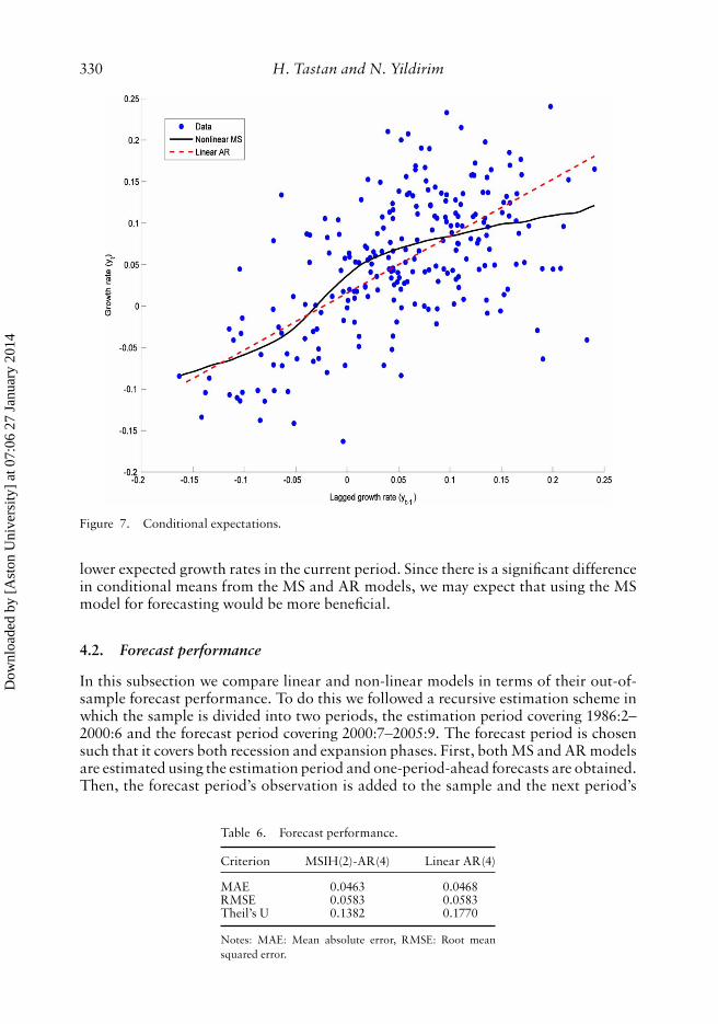
Table 6. Forecast performance.
Criterion MSIH(2)-AR(4) Linear AR(4)
MAE 0.0463 0.0468RMSE 0.0583 0.0583Theil’s U 0.1382 0.1770
Notes: MAE: Mean absolute error, RMSE: Root meansquared error.
Dow
nloa
ded
by [
Ast
on U
nive
rsity
] at
07:
06 2
7 Ja
nuar
y 20
14
International Economic Journal 331
value is forecast. Proceeding recursively in this way, one-period-ahead out of sampleforecast values consisting of 63 observations are obtained.
To compare linear AR(4) and MSIH(2)-AR(4) we computed mean absolute errors(MAE), root mean squared errors (RMSE) and Theil’s U. The forecast performance issummarized in Table 6. The MS and linear models have almost identical MAEs andRMSEs. However, based on the Theil’s U, the Markov Switching model performs betterthan the linear AR model in terms of one-period ahead forecast.
5. Conclusion
This paper investigated the usefulness of non-linear models in detecting business cycleasymmetries in the Turkish industrial production index. Following common practicein the literature, we employed a Markov switching AR framework, which is compati-ble with the finding of cyclical asymmetry. It is shown in the paper that business cycleproperties are sensitive to model components, especially the number of states. In decid-ing between two- versus three-regime MS models, several commonly used and newlydeveloped model selection procedures were employed. To avoid the problem of spuriousregimes, the quality of regime classification was taken as the final criterion to choosethe adequate model. Based on this, a two-regime MS model with regime-dependentvariances and intercepts is chosen for the analysis of business cycle asymmetries. Theestimation results indicate that there are four recessionary and five expansionary peri-ods in the sample. Parametric asymmetry tests indicate that the conditional probabilityof moving from recession to expansion is statistically larger than the conditional prob-ability of moving from expansion to recession. The duration of recessions (expansions)is found to be shorter (longer) than its counterpart in other developing economies. Thecomparison of a non-linear model to a linear autoregressive model using parametricand non-parametric methods imply that the MS model is more successful in capturingasymmetries in Turkish business cycles and in estimating the conditional expectationof the next period’s growth rate. In addition, one-period-ahead out-of-sample forecastsfrom the MS model are better than the linear AR formulation.
Notes
1. A theoretical explanation for the business cycle asymmetry was provided by Acemoglu and Scott (1997). Theyshow that if there are intertemporal increasing returns (resulting from, for example, investment in new technology,innovation, maintenance, learning-by-doing, etc) in an economy, then returns from an activity in this period arehigher if the activity occurred in the recent past leading to persistent periods of low and high growth. Their modelreduces to Hamilton’s MS model under certain conditions.
2. Arango and Melo (2006) provided evidence of business cycle asymmetry for Brazil, Colombia and Mexico usingLSTAR models.
3. There are two official religious holidays: the Festival of Ramadan (three days following the last day of the holymonth of Ramadan) and the Festival of Sacrifice (four days). The exact days change from year to year accordingto the Hijri Calendar. Each year the holidays roll backwards about 10–11 days from the previous year. In someyears the official holidays are as long as five days. This is the reason for using dummy variable regression toremove their effects. The parameter estimate on the dummy variable is −0.0257 with p-value 0.0665.
4. Not reported but available upon request.5. This can be compared, for example, to Arango and Melo (2006) who reported the following speed of adjustment
parameter estimates: 183.49 for Brazil, 69.501 for Colombia and 73.99 for Mexico.6. We have used Ox package MSVAR written by Hans-Martin Krolzig. For more information visit
http://www.kent.ac.uk/economics/staff/hmk/.
Dow
nloa
ded
by [
Ast
on U
nive
rsity
] at
07:
06 2
7 Ja
nuar
y 20
14
332 H. Tastan and N. Yildirim
7. The number of observations used in each of the model is set to T − 12 = 225 in order to make data-basedinformation criteria comparable with each other.
8. Smith et al. (2006) note that one has a 50-50 chance of choosing the right model using the AIC, SIC and HQICto select both the number of regimes and the AR order.
9. For the sake of completeness, the model estimated here is known as the fixed transition probability (FTP)MSIH-AR model. An alternative formulation takes the transition probabilities dependent on time through someinformation variable such as a leading economic indicator index. As discussed in Filardo (1994), the time-varyingtransition probability (TVTP) model for the monthly US industrial production index outperforms the FTP variantin replicating official business cycle dates released by the NBER. If one has access to official business cycle datesthen the correlation between official dates and the model’s predictions can easily be calculated. However, thereis no official business cycle dating mechanism in Turkey, as in the US, that one can use to compare the model’spredictions. We estimated the TVTP variant of the same model using the lagged leading economic indicator indexreleased by the Central Bank of the Republic of Turkey as the information variable for the transition variables forthe adjusted sample of 1988:12–2005:9. In terms of business cycle dates the results from the TVTP and the FTPmodels were almost identical (the results are not reported to save space but are available upon request). Thus, wepreferred to employ the FTP-MSIH(2)-AR(4) model for the rest of the study.
10. The value of ε was chosen as 0.7 and the p-values were obtained by bootstrap using 5000 repetitions.11. Selected countries in this study include South Africa, Malawi, Côte d’Ivoire, Zimbabwe, Uruguay, Columbia,
Peru, Chile, Mexico, India, Korea, Morocco, Pakistan, Malaysia. We note that Rand and Tarp (2002) implementedthe Bry-Boschan (BB) rule to date the business cycles, not the MS models.
12. See also the replication conducted by Belaire-Franch and Contreras (2003).13. Test results are robust to the choice of lag order including zero.
References
Acemoglu, D., and A. Scott. 1997. Asymmetric business cycles: Theory and time-series evidence. Journal of MonetaryEconomics 40: 501–33.
Ang, A., and G. Bekaert. 2002. Regime switches in interest rates. Journal of Business and Economic Statistics 20, no. 2:163–82.
Arango, L.E., and L.F. Melo. 2006. Expansions and contractions in Brazil, Colombia and Mexico: A view throughnonlinear models. Journal of Development Economics 80: 501–17.
Artis, M., H.-M. Krolzig, and J. Toro. 2004. The European business cycle. Oxford Economic Papers 56: 1–44.Belaire-Franch, J., and D. Contreras. 2003. An assessment of international business cycle asymmetries using Clements
and Krolzig’s parametric approach. Studies in Nonlinear Dynamics and Econometrics 6, no. 4: 1–9.Breunig, R., S. Najarian, and A. Pagan. 2003. Specification testing of Markov switching models, Oxford Bulletin of
Economics and Statistics 65: 703–25.Breunig, R., and A. Pagan. 2004. Do Markov-switching models capture nonlinearities in the data? Tests using
nonparametric methods. Mathematics and Computers in Simulation 64: 401–7.Breunig, R., and A. Stegman. 2005. Testing for switching in Singaporean business cycles. Singapore Economic Review
50, no. 1: 25–34.Bry, G., and C. Boschan. 1971. Cyclical analysis of time series: selected procedures and computer programs. New York:
NBER.Camacho, M., and G. Perez-Quiros. 2006. Do European business cycles look like one?, Central Bank of Spain Working
Paper no. 0518.Clements, M.P., and H.-M. Krolzig. 2003. Business cycle asymmetries: Characterization and testing based on Markov-
switching autoregressions. Journal of Business and Economic Statistics 21, no. 1: 196–211.Filardo, A. 1994. Business-cycle phases and their transitional dynamics. Journal of Business and Economic Statistics
12: 293–308.Garcia, R. 1998. Asymptotic null distribution of the likelihood ratio test in Markov switching models. International
Economic Review 39, no. 3: 763–88.Girardin, E. 2005. Growth-cycle features of East Asian countries: Are they similar? International Journal of Finance
and Economics 10: 143–56.Hamilton, J.D. 1989. A new approach to the economic analysis of nonstationary time series and the business cycle.
Econometrica 57, no. 2: 357–84.———. 1994. Time series analysis, 1st edn. Princeton, NJ: Princeton University Press.Hansen, B. 1992. The likelihood ratio test under non-standard conditions: Testing the Markov switching model of
GNP. Journal of Applied Econometrics 7: S61–82.
Dow
nloa
ded
by [
Ast
on U
nive
rsity
] at
07:
06 2
7 Ja
nuar
y 20
14
International Economic Journal 333
Harding, D., and A. Pagan. 2002. A comparison of two business cycle dating methods. Journal of Economic Dynamicsand Control 27: 1681–90.
Hess, G.D., and S. Iwata. 1997. Asymmetric persistence in GDP? A deeper look at depth. Journal of Monetary Economics40: 535–54.
Kapetanios, G. 2001. Model selection in threshold models. Journal of Time Series Analysis 22, no. 6: 733–54.Krolzig, H.-M. 1997. Markov-switching vector autoregressions: Modelling, statistical inference and an application to
the business cycle analysis. Lecture Notes.———. 2001a. Business cycle measurement in the presence of structural change: International evidence. International
Journal of Forecasting 17: 349–368.———. 2001b. Markov-switching procedures for dating the euro-zone business cycle. Vierteljahrshefte zur Wirtschafts-
forschung 70: 339–51.Krutz, M. 2005. A three-regime business cycle model for an emerging economy. Applied Economics Letters 12: 399–402.Lam, P.-S. 2004. A Markov-switching model of GNP growth with duration dependence. International Economic Review
45, no. 1: 175–204.McQueen, G., and S. Thorley. 1993. Asymmetric business cycle turning points. Journal of Monetary Economics 31:
341–62.Moolman, E. 2004. A Markov switching regime model of the South African business cycle. Economic Modelling 21:
631–46.Neftci, S.N. 1982. Optimal prediction of cyclical downturns. Journal of Economic Dynamics and Control 4: 225–41.Newey, W.K., and K.D. West. 1987. A simple, positive semi-definite, heteroscedasticity and autocorrelation consistent
covariance matrix. Econometrica 55, no. 3: 703–8.Psaradakis, Z., and N. Spagnolo. 2003. On the determination of the number of regimes in Markov-switching
autoregressive models. Journal of Time Series Analysis 24, no. 2: 237–52.Rand, J., and F. Tarp. 2002. Business cycles in developing countries: Are they different? World Development 30, no. 12,
2071–2088.Sichel, D.E. 1993. Business cycle asymmetry: A deeper look. Economic Inquiry 31, no. 2: 224–36.Smith, A., P.A. Naik, and C.-L. Tsai. 2006. Markov-switching model selection using Kullback–Leibler divergence.
Journal of Econometrics 134, no. 2: 553–577.Taylor, A., D. Shepherd, and S. Duncan. 2005. The structure of the Australian growth process: A Bayesian model
selection view of Markov switching. Economic Modelling 22: 628–645.Terasvirta, T. 1994. Specification, estimation and evaluation of smooth transition autoregressive models. Journal of
the American Statistical Association 89, no. 425, 208–18.Zhang, J., and R.A. Stine. 2001. Autocovariance structure of Markov regime switching models and model selection.
Journal of Time Series Analysis 22, no. 1: 107–24.