This PDF is a selection from an out-of-print volume from the National Bureauof Economic Research

Volume Title: Business Cycles: Theory, History, Indicators, and Forecasting

Volume Author/Editor: Victor Zarnowitz

Volume Publisher: University of Chicago Press

Volume ISBN: 0-226-97890-7

Volume URL: http://www.nber.org/books/zarn92-1

Conference Date: n/a

Publication Date: January 1992

Chapter Title: Consensus and Uncertainty in Economic Prediction

Chapter Author: Victor Zarnowitz

Chapter URL: http://www.nber.org/chapters/c10388

Chapter pages in book: (p. 492 - 518)

17 Consensus and Uncertainty inEconomic Prediction

17.1 Concepts and Problems

Although all forecasts are by their very nature probabilistic statements,most economic predictions quote but a single value to be assumed by a certainvariable, without specifying the attached probabilities. Often many such pointforecasts are available for a given target variable from a business outlook sur­vey. If they show a high degree of agreement, does this indicate that the fore­casters confidently expect the outcome they commonly predict to come true?More generally, does the dispersion of the point forecasts reflect their authors'uncertainty (i.e., their relative lack of confidence)? This paper deals withthese and other related questions, drawing on a set of data that is very rare ineconomics in that it includes related point and probabilistic forecasts from thesame sources.

17 .1. 1 Consensus

Averages from economic outlook surveys are frequently called "consensus"forecasts or treated as such. The term has entered the popular discourse with­out having been defined in a generally accepted way. But it is clear that thedegree to which a survey average is representative of the collected individualpredictions can vary greatly depending on the nature of the underlying distri­bution. There may be no meaningful consensus if the distribution of the point

This chapter is co-authored with Louis A. Lambros and is reprinted from the Journal ofPoliticalEconomy 95 (June 1987): 591-621. © 1987 The University of Chicago. All rights reserved.

The authors are much indebted for helpful comments on an earlier draft of this paper to JamesHeckman and two anonymous referees. They also thank Walter Baehrend, Douglas Scott Katzer,Walter R. Teets, and Christine Verhaaren for efficient help with research and typing. Financialsupport from the National Science Foundation to the National Bureau of Economic Research (NSFgrant SES-792036l) and aid from the Graduate School of Business of the University of Chicagoare gratefully acknowledged. Any remaining errors are those of the authors.

492

493 Consensus and Uncertainty in Economic Prediction

forecasts in question is highly diffuse or multimodal because of large differ­ences among the underlying models. On the other hand, a consensus wouldbe strongly in evidence for any unimodal, symmetrical, and sufficiently tightdistribution (see Schnader and Stekler 1979). The inverse aspect of the con­sensus is the dispersion of a sample of point forecasts, which can be measuredsimply by their standard deviation.

In predicting the value an aggregate variable is to assume in a given period,individuals and groups use in part the same public information and the sameestablished techniques and relationships. The common elements induce somepositive correlation across the resulting forecasts. Insofar as the makers andusers of the forecasts interact and influence each other, directly or indirectly,the correlation of corresponding expectations would be reinforced. That suchinterdependencies may be substantial is suggested by the existence of infor­mal exchanges and organized polls of opinion, market arrangements for thesale of expert advice, and media dissemination of public forecasts. A fre­quently encountered surmise is that many forecasters are risk averters who donot wish to deviate much at any time from the views of the future that appearto be prevalent. If so, the distribution of the approximately contemporaneouspoint forecasts for a given target would be further tightened around an influ­ential "consensus" value.

But there are also important limitations and countertendencies to this pro­cess. Only the hypothetical expectations containing all the pertinent informa­tion generated in the economy are necessarily self-fulfilling; actual forecasts,even if widely shared, are not since they are inevitably based on partial andimperfect knowledge. No mechanism has been discovered to ensure the con­vergence of the forecasts to a unique and stable equilibrium path. Attempts topredict average opinion or what others are likely to predict that average to beand so forth run into the frustrating "infinite regress" problem. Certainly, gen­uine predictions intended to guide the decision making or affect views in themarketplace do not merely mimic one another. Thus simple averages of fore­casts from successive business outlook surveys have proved to be more accu­rate over time, and also less biased, than most of the corresponding forecastsets of the individual participants. Evidently there is a good deal of indepen­dent information in the individual forecast series so that their collinearity islimited, and combining them yields net gains in predictive power (Zarnowitz1967, pp. 123-26; 1984a; 1985a).1

17.1.2 Uncertainty

In a number of recent studies, which are cited below, high (low) dispersionof predicted price changes across survey respondents is interpreted as being

1. On methods to choose a diversified "portfolio" of forecasts and weights that reduce thevariance of the resulting composite, see Bates and Granger 1969 and Newbold and Granger 1974.On the conditions under which unweighted aggregate predictions are optimal or nearly optimal,see Einhorn and Hogarth 1975 and Hogarth 1978.

494 Chapter Seventeen

indicative of high (low) "inflation uncertainty." Thus uncertainty is heresimply identified with the inverse of what was labeled "consensus" in the pre­ceding subsection.

It is important to recognize that this approach does not involve any directmeasurement of uncertainty in the usual sense of that term. The latter is afunction of the distribution of the probabilities that a forecaster attaches to thedifferent possible outcomes (values) of the predicted event (variable). Thetighter this distribution, the lower is the associated uncertainty.

For an informed outside assessment of uncertainty so defined, therefore,some sufficient knowledge of the probabilities involved would seem neces­sary. Inferences from point forecasts do not produce such knowledge; theymayor may not provide helpful clues in its absence. When the standard devia­tion of a set of corresponding predictions by different individuals is taken toindicate uncertainty, the underlying assumption is that this interpersonal dis­persion measure is an acceptable proxy for the dispersion of intrapersonalpredictive probabilities or beliefs held by the same individuals. The validityof this assumption can by no means be taken for granted; it is an empiricalquestion that is best answered by direct measurement and testing.

Some events do have stable and known distributions of outcomes; others donot. It is generally easier to predict stationary than nonstationary variables,transitory than permanent changes, smooth trends than abrupt turning points.The stabler and more knowable the underlying "objective" probability distri­butions are, the greater presumably is the accuracy of the forecasts and theconfidence with which the subjective probabilities of the predicted outcomesare held. The concept of uncertainty adopted here applies in principle toany probabilistic forecast, whether held with a high or a low degree of confi­dence. 2

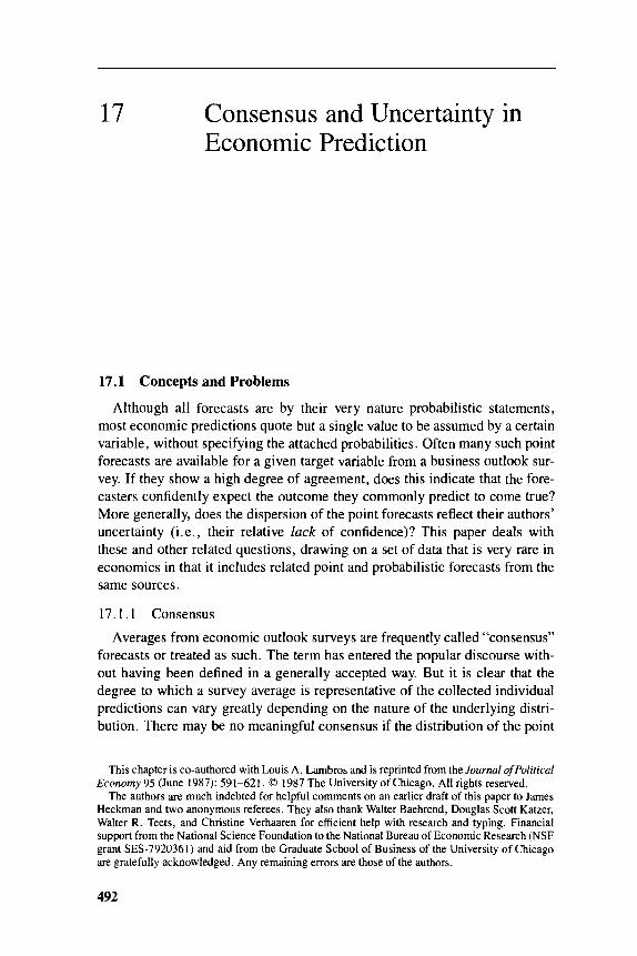
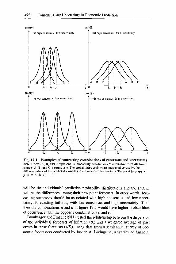
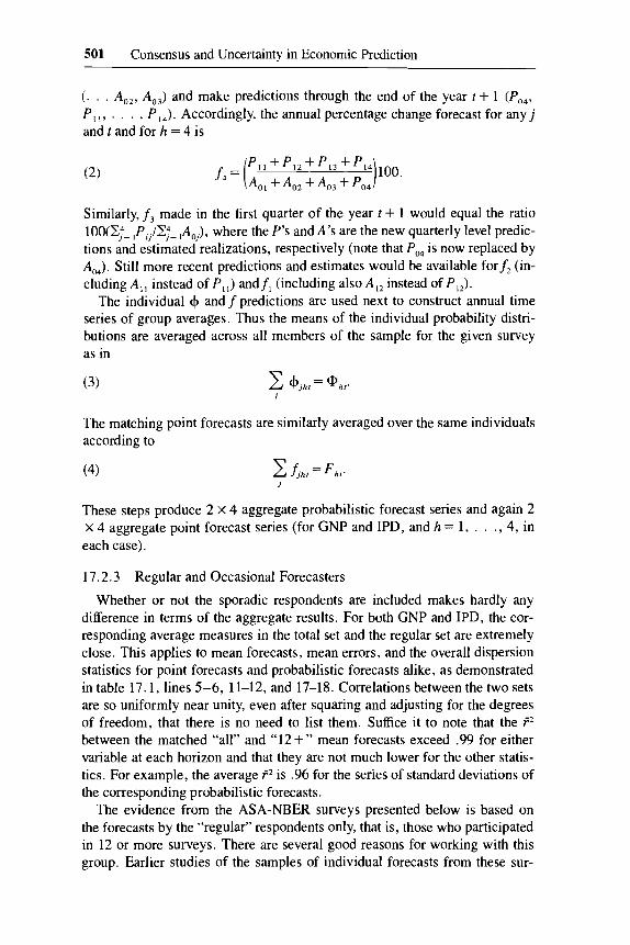
Simple schematic diagrams suffice to show the important distinction be­tween consensus and uncertainty and how the two may be related. In figure17.1 the point forecasts reported by the individuals A, B, and C are viewed asthe expected values of their respective probability distributions. The degree ofconsensus among the three (or any number of) survey respondents is said tobe "high" when their point forecasts are clustered, "low" when they arewidely dispersed. The degree of uncertainty is said to be high when the pre­dictive distributions of A, B, C, ... are diffuse, low when they are tight. Asillustrated in panels a and b of the figure, high consensus may be associatedwith either low or high uncertainty. Similarly, low consensus may be asso­ciated with either low or high uncertainty (panels c and d).

Suppose, however, that both uncertainty and consensus depend on the ac­curacy record of the recent point forecasts. The better that record, the tighter

2. Thus no use is made in this paper of the distinction between "risk" and "uncertainty" (Knight1921; Keynes 1936), which has important implications in other contexts (chapter 2; Meltzer1982).

495 Consensus and Uncertainty in Economic Prediction

prob(y) prob(y)

(a) high consensus, low uncertainty (b) high consensus, high uncertainty

y

ABCABC

y 0

prob(y)

(d) low consensus, high uncertainty(c) low consensus, low uncertainty

y

Fig. 17.1 Examples of contrasting combinations of consensus and uncertaintyNote: Curves A, B, and C represent the probability distributions of alternative forecasts fromsources A, B, and C, respectively. The probabilities prob(y) are measured vertically; thedifferent values of the predicted variable (y) are measured horizontally. The point forecasts areYi' (i = A, B, C, ...).

will be the individuals' predictive probability distributions and the smallerwill be the differences among their new point forecasts. In other words, fore­casting successes should be associated with high consensus and low uncer­tainty; forecasting failures, with low consensus and high uncertainty. If so,then the combinations a and d in figure 17.1 would have higher probabilitiesof occurrence than the opposite combinations band c.

Bomberger and Frazer (1981) tested the relationship between the dispersionof the individual forecasts of inflation (J" t) and a weighted average of pasterrors in these forecasts (Y"Sr), using data from a semiannual survey of eco­nomic forecasters conducted by Joseph A. Livingston, a syndicated financial

496 Chapter Seventeen

columnist. 3 They found a high positive correlation (r2 = .77) between the twomeasures, which they argued supports the use of O't as a proxy for inflationuncertainty. However, this result, though suggestive, is inconclusive. Pastforecast errors represent only one of the presumptive determinants of uncer­tainty; others, more future-oriented, are at least as important. They includethe latest readings on the various influential indicators, the recent trends andprospective shifts in economic policies, and changes in the external factorsaffecting business and finance. Each of these is a source of signals that oftendiverge and are subject to different interpretations, and hence of uncertainty.

There is also a statistical problem here: the serial correlation of errors fromthe Livingston survey predictions could well account for much of the associa­tion between O't and v'Sr. The predominant finding from a number of studiesof inflation forecasts is that they generally fail the conventional tests of un­biasedness, efficiency, or consistency. 4

17.1.3 Hypotheses and Tests

For any time series, increased volatility tends to be associated with de­creased predictability. Thus the more variable inflation is, the less of it will beanticipated. But when inflation rises to unusually high levels, it is likely tobecome more volatile. Repeated policy attempts (a) to keep unemploymentlow by stimulating spending and (b) to counter the resulting intermittentbursts of inflation inevitably produce monetary instability. People increasinglyrealize how this process works, and so anticipated inflation will rise and be­come more variable, augmenting uncertainty.

Extensions of this hypothesis attribute adverse real effects to such develop­ments. High and volatile inflation raises frictions in the markets and lowersproductivity. Prior contracts delay adjustments toward shorter commitmentsand more indexation. The effectiveness of relative prices in guiding and coor­dinating economic actions is impaired as distinguishing signals from noise inthe observed absolute prices becomes increasingly difficult. These argumentshave been used in attempts to explain positive comovements of inflation and

3. Livingston's June and December columns, published in the Philadelphia Bulletin and thePhiladelphia Inquirer, refer to the levels of the predicted variables 6 and 12 months hence. Theinitially published average forecasts contain frequent adjustments intended to allow for largechanges in the data between collection and publication. Carlson (1977) concluded that these ad­justments cannot be justified, and he eliminated them by reworking the averages from the originalindividual forecasts. The effective spans of the forecasts were now assumed to be 8 and 14months. Subsequent research work generally relied on the means and standard deviations of theLivingston forecasts in the form published by Carlson. Bomberger and Frazer used these data forthe 8-month forecasts in 1952-77. Their Sf measure is an average of squared past errors of theindividual forecasts with a geometrically weighted lag distribution.

4. On the evidence for the Livingston data, see Pesando 1975, Carlson 1977, Wachtel 1977,Pearce 1979 and Figlewski and Wachtel 1981 (more favorable results are reported in Mullineaux1978, 1980a). On the evidence from other surveys of economists, consumers, and business exec­utives, see also de Leeuw and McKelvey 1981, Gramlich 1983, and Zamowitz 1985a.

497 Consensus and Uncertainty in Economic Prediction

unemployment rates as in the "stagflation" of the 1970s (M. Friedman 1977),as well as the role of monetary shocks and price misperceptions in businesscycles (Lucas 1975, 1977).

Evidence from actual price index data on the whole supports the idea that apositive relationship exists between the rate of inflation and its variability overtime (R. J. Gordon 1971; Okun 1971; B. Klein 1975). Additional supportcomes from international cross-section studies that suggest that countries withhigher average rates of inflation tend to have higher standard deviations ormean absolute changes of inflation (Logue and Willett 1976; Jaffee and Klei­man 1977; Foster 1978).

Wachtel (1977) shows that the inflation expectations of economists and con­sumers (collected by Livingston and the Survey Research Center of the Uni­versity of Michigan, respectively) have had large errors, mostly of underesti­mation. Nevertheless, these data contribute to equations for consumption,prices, wages, and interest rates when used along with other determinants (forsome qualifications, see de Menil 1977). Cukierman and Wachtel (1979) findthat for both of these surveys, the variance of inflation predictions across therespondents increases with the variance of measured inflation.

According to Mullineaux (1980b), the unemployment rate Utfalls with the

unexpected part of the current inflation rate, 1T~ = 1T t -1T~, and rises with (J't-i

and Ut - j , where 1T~ and (J't are Carlson estimates of means and standard devia­tions of the Livingston survey forecasts, and the lags i = 0, ... , 11 and j =0, . . . , 4 years. However, the interpretation of these equations is difficultbecause of the use of long distributed lags in the presence of highly autocor­related variables, notably U and (J'. The cumulative effects on U of (J' and,especially, 1T" are weak in the sense that they require long lags to get signifi­cantly large with the expected signs.

In Levi and Makin 1980, the percentage change in employment dNt

de­pends positively on 1T~ and inversely on (J't. The equations yield significantlypositive correlations only when (J't is included. 5 Makin (1982) relates dNt , orits counterpart for output, to "anticipated" and "unanticipated" money growthrates, current and lagged, and to (J't-i' i = 0, 1. Again, inflation uncertaintyrepresented by (J' is found to act as a significant depressant (the other conclu­sion is that anticipated money has substantial initial effects in stimulating realeconomic activity). These studies do not rely critically on distributed lags andare therefore more convincing.

Expectational data from the same surveys have also been used in severalrecent studies of the determinants of nominal yields (it) on bonds free of de­fault risk. Here typically a reduced-form "Fisher equation" is estimated,where i depends on 1Te , (J', and some factors affecting aggregate demand and

5. For 1948-75, however, the R2 coefficients are low, about .1-.2. For 1965-75, a period ofrising and more variable inflation, they are much higher: near or above .6.

498 Chapter Seventeen

supply such as exogenous expenditures and money growth rates (or sur­prises).6 Levi and Makin (1979), Bomberger and Frazer (1981), and Makin(1983) present regression estimates that show that the interest rates are nega­tively influenced by the current values of (J't or distributed lags in this variable.However, Bamea, Dotan, and Lakonishok (1979) and Brenner and Lands­kroner (1983) report positive coefficients of (J' or related proxies, while Melvin(1982) has a positive but not significant coefficient, which he suggests may bedue to defects of the survey measure and the consequent errors-in-variablesbias toward zero.

These apparently contradictory results may merely indicate that the sign ofthe effect of (J' on i is not clear. The argument is that inflation uncertaintydepresses both real investment and savings as borrowers and lenders are dis­couraged by expected volatility of relative and absolute prices. If the impacton investment dominates, the net effect of (J' on the after-tax real rate andhence on i will be negative; if the impact on savings dominates, that effect willbe positive (Makin 1983).

The models under review are products of the 1970s, a period of rising infla­tion; it is not clear that they pass the test of the disinflation in the 1980s. Thesharp decline in actual inflation was accompanied by less volatility of pricechange. There can be little doubt that it induced lagging but substantial reduc­tions in expected inflation and presumably also in the associated uncertainty.Yet, even when real growth was positive, the rates of productivity, investment,and saving remained on the whole low in these years (puzzlingly so to manyobservers), except for the strong but brief recovery in 1983-84. Interest ratesdeclined generally but much less than inflation. 7 Recent attempts to explainthese developments rely on various special factors.

17.1.4 Further Steps

Evidently, economics of uncertainty is an important and active field ofstudy, with interest centering on inflation. 8 Just as clearly, there is as yet littlewell-tested knowledge about it.

The approach to be followed here is to elicit information on uncertaintyfrom time series of probabilistic forecasts. Section 17.2 presents the data andmeasures we have developed.

6. Some of these studies also consider the roles of taxes, real rates, and lags, whereas othersare limited to the gross effects on it of net and (J't or related measures. For comprehensive surveysof the literature, see Tanzi 1984.

7. Note that the downward movement of the rates occurred entirely during the recessions of1980 and 1981-82 as well as the slowdown after mid-1984; it was interrupted and partially re­versed in the intervening recoveries.

8. Uncertainty about real growth prospects has received little attention in recent literature. Theeffects of changes in the "confidence" of consumers, investors, and business people are oftenemphasized, but these changes themselves and their determinants are extremely difficult to mea­sure and analyze. What is needed here is probabilistic forecasts for real economic activity. Oursurveys provide such materials but only since mid-1981 (see sec. 17.2).

499 Consensus and Uncertainty in Economic Prediction

Section 17.3 discusses the results based on these materials and comparesthem with the results obtained by means of the point forecast proxies for un­certainty. This is presumably the best way to answer the empirical question ofjust how well the indirect measures have worked. The use of matched proba­bilistic and point forecast sets allows us to examine directly how consensusand uncertainty are related and also whether expectations of higher inflationbreed more inflation uncertainty (secs. 17.3.1-17.3.4). Next we explore waysto bring together the measures derived from our series of probabilistic forecastdistributions and the measures derived from the Livingston point forecastdata. This cross-section analysis is then extended to reexamine the hypothesesdiscussed above on how inflation uncertainty affects real economic activityand inflation rates (secs. 17.3.5-17.3.7).

Section 17.4 sums up our conclusions.

17.2 Data and Measures

17.2.1 Properties of Surveys and Samples

The survey conducted quarterly since 1968 by the American Statistical As­sociation (ASA) and the National Bureau of Economic Research (NBER) is,to our knowledge, unique in regularly yielding numerical replies on predictiveuncertainty. A questionnaire, mailed to a broadly based and diversified list ofpersons who are professionally engaged in the analysis of current and pro­spective business conditions, asks for forecasts on a number of importantmacroeconomic variables including the gross national product in current dol­lars (GNP) and in constant dollars (RGNP) and the GNP implicit price deflator(IPD). These predictions refer to the current and the next four quarters and tothe current and next year.

In addition to these point forecasts, the ASA-NBER survey provides prob­abilistic forecasts for IPD and GNP (through mid-1981) and for IPD andRGNP (thereafter). For each of the paired variables, a list of percentage inter­vals (e.g., 10.0-10.9, 9.0-9.9, etc.) is included, with blank spaces to writethe numbers in. The replies represent the chances in 100 that the forecasterassociates with the changes falling in the selected intervals.

Although the numbers refer to annual changes, they come from quarterlysurveys so that the effective horizons of the predictions vary substantially. Ofprincipal interest are the probabilistic forecasts for the change from year t - 1to year t that were issued in the four consecutive surveys from the last quarterof t - 1 through the third quarter of t. The distances between the dates of thesesurveys and the end of the target year are approximately 4V2, 3V2, 2V2, and1V2 quarters. We shall refer to these categories simply as horizons (H) 4, ..., 1. They account for the bulk of the more than 4,600 reported probabilisticforecast distributions for 1969-81 and can be regularly matched with thepoint forecasts made by the same persons for the same targets.

(1)

500 Chapter Seventeen

The total number of persons who responded to any of the 51 ASA-NBERsurveys taken during the period 1968:4-1981:2 is 192; the number of thosewho participated in at least 12 surveys is 80. The latter subset of "regular"respondents is the main source of evidence in this paper, but we analyzed thetotal set as well to make sure that the selection does not bias our results in anyparticular way.

Data from the completed questionnaire forms available in the NBER fileswere screened so as to (1) strictly match the probabilistic and point forecastsmade by the same persons for the same targets and (2) eliminate unusablereplies and obvious reporting errors. The last step improved the quality ofmicrodata in our sample but had minimal effects on the aggregate measuresobtained since the proportion of the forecasts excluded was very small.

The final collection for the group of regular forecasters includes 1,673 and1,705 individual probability distributions for GNP and IPD, respectively. Theshortest forecasts (HI) account for about 19% of these data, H2 for 27%, H3for 28%, and H4 for 26%.9

17.2.2 Aggregate Probabilistic and Point Forecast Series

Summary statistics such as the mean, standard deviation, skewness, andkurtosis were calculated for each of the individual probability distributions. 10

Uniform distribution within each of the selected intervals was assumed. Thusthe kth-order moment about zero of the distribution is computed by numericalintegration as

(U~+l l~+l)

IJ.~= ~ Pi k~ 1 - k'+ 1 '

where Pi is the probability assigned to the ith interval (~iPi = 1), and 1i and Uiare the lower and upper limits of the ith interval, respectively. Since unit inter­vals are used, the mean (k = 1) reduces to ~iPJ(li + ui)/2]. The mean forecastimplicit in the jth respondent's probability distribution for horizon h and yeart will be denoted as <Pjht •

For each <Pjht there is a matching point forecast ~ht. The latter numbers arecomputed from corresponding estimates and predictions of quarterly levelsof GNP and IPD. For example, in the fourth quarter of year t04 ' a respond­ent would use data on the "actual" values of GNP in the preceding quarters

9. The probabilistic predictions issued in the second and third quarters of year t - 1 (H6 andH5) and in the fourth quarter of year t (HO) are excluded. Such replies are available only for theyears 1974, 1980, and 1981. Also, only 136 (about half) of them have point counterparts. Theprobabilistic distributions with the horizons of 6 and 5 quarters cannot be matched with pointforecasts at all, and those with the zero horizon lack interest since by the fourth quarter of t mostof the target year is already over. In addition, 210 faulty or unusable replies were eliminated byediting the questionnaires for degenerate distributions with single "100" entries (116), cases inwhich the probabilities do not add up to 1.00 (47), and mistaken applications to real rather thannominal GNP (47).

10. The results reported below are not affected by skewness and kurtosis, and no use will bemade of these measures in this paper.

501 Consensus and Uncertainty in Economic Prediction

(. . . A02 ' A03 ) and make predictions through the end of the year t + 1 (P04'

P II' .•. , P 14)· Accordingly, the annual percentage change forecast for any jand t and for h = 4 is

(2)

Similarly, /3 made in the first quarter of the year t + 1 would equal the ratio100(~1= IPij/~J= lAo), where the P's and A's are the new quarterly level predic­tions and estimated realizations, respectively (note that P04 is now replaced byA04). Still more recent predictions and estimates would be available for /2 (in­cluding All instead of P ll ) and!l (including also A l2 instead of P12).

The individual <p and! predictions are used next to construct annual timeseries of group averages. Thus the means of the individual probability distri­butions are averaged across all members of the sample for the given surveyas in

(3) L <pjht = <I> ht·j

The matching point forecasts are similarly averaged over the same individualsaccording to

(4) L~ht=Fht·j

These steps produce 2 x 4 aggregate probabilistic forecast series and again 2x 4 aggregate point forecast series (for GNP and IPD, and h = 1, . . ., 4, ineach case).

17.2.3 Regular and Occasional Forecasters

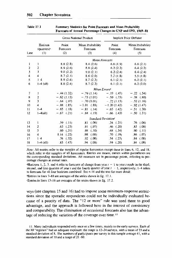
Whether or not the sporadic respondents are included makes hardly anydifference in terms of the aggregate results. For both GNP and IPD, the cor­responding average measures in the total set and the regular set are extremelyclose. This applies to mean forecasts, mean errors, and the overall dispersionstatistics for point forecasts and probabilistic forecasts alike, as demonstratedin table 17.1, lines 5-6, 11-12, and 17-18. Correlations between the two setsare so uniformly near unity, even after squaring and adjusting for the degreesof freedom, that there is no need to list them. Suffice it to note that the f2between the matched "all" and "12 +" mean forecasts exceed .99 for eithervariable at each horizon and that they are not much lower for the other statis­tics. For example, the average f2 is .96 for the series of standard deviations ofthe corresponding probabilistic forecasts.

The evidence from the ASA-NBER surveys presented below is based onthe forecasts by the "regular" respondents only, that is, those who participatedin 12 or more surveys. There are several good reasons for working with thisgroup. Earlier studies of the samples of individual forecasts from these sur-

502 Chapter Seventeen

Table 17.1 Summary Statistics for Point Forecasts and Mean ProbabilityForecasts of Annual Percentage Changes in GNP and IPD, 1969-81

Gross National Product Implicit Price Deflator

Horizon Point Mean Probability Point Mean Probability(quarters )a Forecasts Forecasts Forecasts Forecasts

Line (1) (2) (3) (4) (5)

Mean Forecasts1 1 8.8 (2.8) 8.4 (2.6) 6.6 (1.9) 6.6 (2.1)2 2 8.9 (2.6) 8.8 (2.4) 6.2 (2.2) 6.4 (2.2)3 3 9.0 (2.2) 9.0 (2.1) 6.2 (2.4) 6.4 (2.4)4 4 8.7(2.1) 8.6 (2.0) 5.2 (1.8) 5.5 (1.8)5 1-4 8.9 (2.4) 8.7 (2.3) 6.1 (2.1) 6.2 (2.1)6 1-4 (all) 8.8 (2.4) 8.7 (2.3) 6.1 (2.1) 6.2 (2.0)

Mean Errorsb

7 1 -.44 (1.32) - .79 (1.14) -.19 (.47) -.22 (.54)8 2 - .62 (1.13) - .73 (1.01) -.50 (.73) - .38 (.80)9 3 -.64 '(.97) - .70 (1.01) -.72(1.13) - .52 (1.16)

10 4 - .88 (.85) -1.01 (.88) - 1.20 (1.42) - .92 (1.47)11 1-4 - .65 (.18) -.81 (.14) -.65 (.42) -.51 (.30)12 1-4(all) -.67 (.21) -.84 (.19) -.66 (.43) -.50 (.31)

Standard Deviationc

13 1 .39 (.11) .81 (.06) .34 (.21) .76 (.06)14 2 .63 (.23) .91 (.07) .46 (.20) .83 (.08)15 3 .90 (.31) .98 (.10) .68 (.34) .90 (.11)16 4 1.14 (.22) .98 (.08) .70 (.19) .86 (.07)17 1-4 .76 (.32) .92 (.08) .54 (.23) .84 (.08)18 1-4 (all) .83 (.43) .94 (.08) .59 (.20) .84 (.08)

Note: All entries refer to the samples of regular forecasters except those in lines 6, 12, and 18,which refer to the samples of all forecasters. Entries are means; entries within parentheses arethe corresponding standard deviations. All measures are in percentage points, referring to per­centage changes at annual rates.aHorizons 1, 2, 3, and 4 refer to forecasts of change from year t - 1 to year t made in the third,second, and first quarters of year t and the fourth quarter of year t - 1, respectively; 1-4 refersto forecasts for all four horizons combined. See n.14 and the text for more detail.bEntries in lines 7-10 are averages of the series shown in fig. 17.1.

cEntries in lines 13-16 are averages of the series shown in fig. 17.2.

veys (see chapters 15 and 16) had to impose some minimum-response restric­tions since the sporadic respondents could not be individually evaluated be­cause of a paucity of data. The "12 or more" rule was used there to goodadvantage, and the approach is followed here in the interest of consistencyand comparability. The elimination of occasional forecasts also has the advan­tage of reducing the variation of the coverage over time. 11

11. Many individuals responded only once or a few times, mainly to the early surveys. Each ofthe 80 "regulars" had an adequate exposure: the range is 12-34 surveys, with a mean of 23 and astandard deviation of 8. The numbers of participants per survey in this sample average 41, with astandard deviation of 10 and a range of 21-60.

503 Consensus and Uncertainty in Economic Prediction

17.3 Results

17 .3.1 Mean Forecasts and Errors

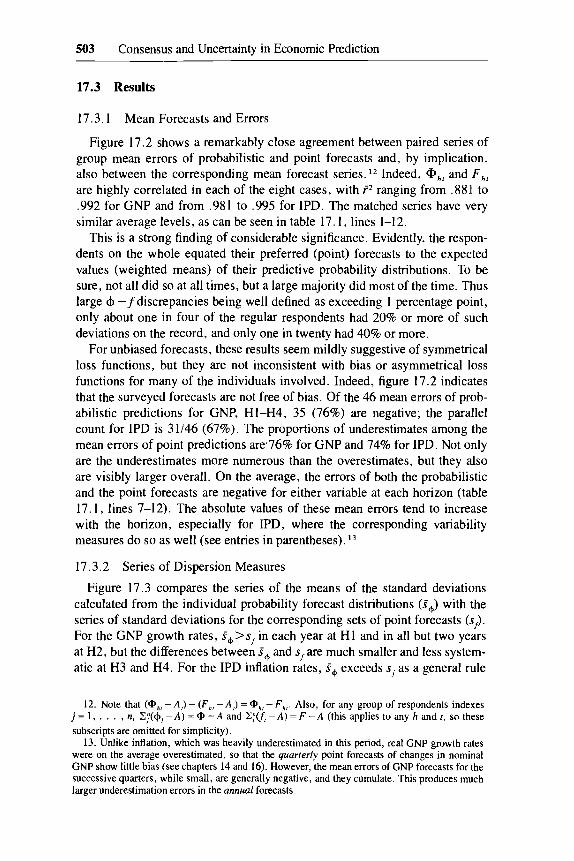
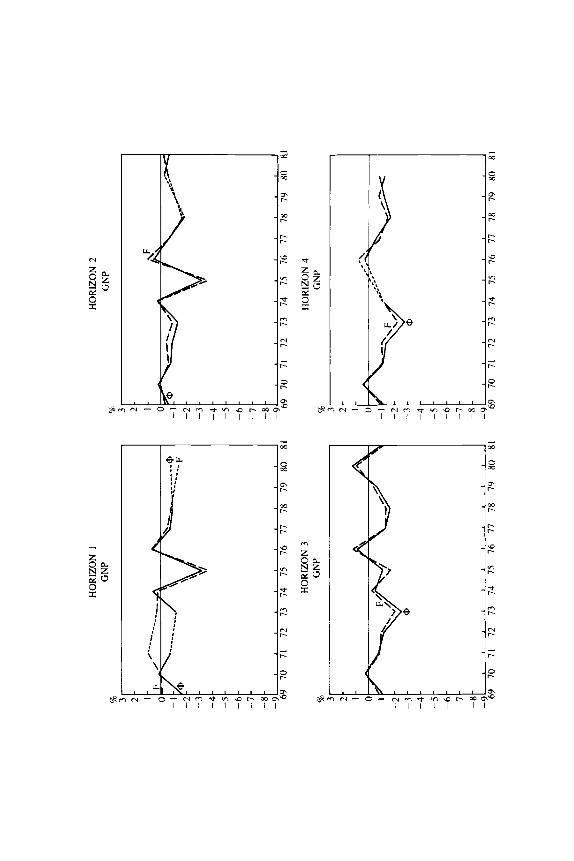
Figure 17.2 shows a remarkably close agreement between paired series ofgroup mean errors of probabilistic and point forecasts and, by implication,also between the corresponding mean forecast series. 12 Indeed, <l>ht and F ht

are highly correlated in each of the eight cases, with ;2 ranging from .881 to.992 for GNP and from .981 to .995 for IPD. The matched series have verysimilar average levels, as can be seen in table 17. 1, lines 1-12.

This is a strong finding of considerable significance. Evidently, the respon­dents on the whole equated their preferred (point) forecasts to the expectedvalues (weighted means) of their predictive probability distributions. To besure, not all did so at all times, but a large majority did most of the time. Thuslarge <f> - f discrepancies being well defined as exceeding 1 percentage point,only about one in four of the regular respondents had 20% or more of suchdeviations on the record, and only one in twenty had 40% or more.

For unbiased forecasts, these results seem mildly suggestive of symmetricalloss functions, but they are not inconsistent with bias or asymmetrical lossfunctions for many of the individuals involved. Indeed, figure 17.2 indicatesthat the surveyed forecasts are not free of bias. Of the 46 mean errors of prob­abilistic predictions for GNP, HI-H4, 35 (76%) are negative; the parallelcount for IPD is 31/46 (67%). The proportions of underestimates among themean errors of point predictions are'76% for GNP and 74% for IPD. Not onlyare the underestimates more numerous than the overestimates, but they alsoare visibly larger overall. On the average, the errors of both the probabilisticand the point forecasts are negative for either variable at each horizon (table17.1, lines 7-12). The absolute values of these mean errors tend to increasewith the horizon, especially for IPD, where the corresponding variabilitymeasures do so as well (see entries in parentheses). 13

17 .3.2 Series of Dispersion Measures

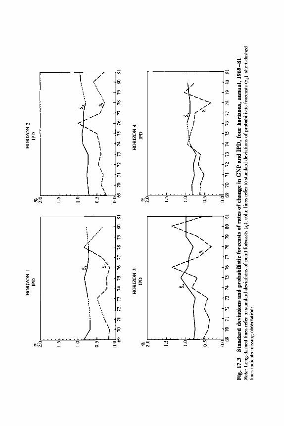
Figure 17.3 compares the series of the means of the standard deviationscalculated from the individual probability forecast distributions (s <f» with theseries of standard deviations for the corresponding sets of point forecasts (sf).For the GNP growth rates, S<f> > Sf in each year at HI and in all but two yearsat H2, but the differences between s<f> and Sf are much smaller and less system­atic at H3 and H4. For the IPD inflation rates, s<f> exceeds Sj as a general rule

12. Note that (<I>ht - At) - (Fht - At) = <l>ht - F ht. Also, for any group of respondents indexesj = 1, ... , n, ~j(<f>.i - A) = <I> - A and ~j({, - A) = F - A (this applies to any hand t, so these

subscripts are omitted for simplicity).13. Unlike inflation, which was heavily underestimated in this period, real GNP growth rates

were on the average overestimated, so that the quarterly point forecasts of changes in nominalGNP show little bias (see chapters 14 and 16). However, the mean errors of GNP forecasts for thesuccessive quarters, while small, are generally negative, and they cumulate. This produces muchlarger underestimation errors in the annual forecasts.

HO

RIZ

ON

1H

OR

IZO

N2

GN

PG

NP

%%

33

22

11

00

-I

':::.:::::

1-1

-2-2

-3-3

-4-4

-5-5

-6-6

-7-7

-8-8

-9-9

6970

7172

7374

7576

7778

7980

8169

7071

7273

7475

7677

7879

808.1

HO

RIZ

ON

3H

OR

IZO

N4

%G

NP

%G

NP

33

22

1

~br

".....

._,0

..._.f:

'::'"

-I

-I~--

-2-2

-3<t>

-3,

<t>-4

-4-5

-5-6

-6-7

-7-8

-8-9

-969

7071

7273

7475

7677

7879

8081

6970

7172

7374

7576

7778

7980

81

HO

RIZ

ON

1H

OR

IZO

N2

%IP

D%

IPD

33

22

1<t>

10

..~-------

..01_7~th

:7/-

...

ep----

-....

...~~::::::::=;.-

--I

<t>-I

-2-2

-3-3

-4-4

-5-5

-6-6

-7-7

-8-8

-9-9

6970

7172

7374

7576

7778

7980

8169

7071

7273

7475

7677

7879

8081

HO

RIZ

ON

3H

OR

IZO

N4

%IP

D%

IPD

33

22

11

<t>I'

;'0

0I

'-.:

"-I

-I

"~

II...

...-=

--"

'I

-2-2

,;, I, I,

-3-3

I,'I I,

-4II

-4I, ~I

-5-5

-6-6

-7-7

-8-8

-969

-970

7172

7374

7576

7778

7980

8169

7071

7273

7475

7677

7879

8081

Fig.

17.2

Mea

ner

rors

inpo

inta

ndpr

obab

ilis

tic

fore

cast

sof

rate

sof

chan

gein

GN

Pan

dIP

D,

four

hori

zons

,an

nual

,19

69-8

1N

ote:

Lon

g-da

shed

line

sre

fer

tom

ean

erro

rso

fgr

oup

fore

cast

s(F

h);

soli

dli

nes

refe

rto

mea

ner

rors

of

grou

ppr

obab

ilis

tic

fore

cast

s(<

I>h);

shor

t-da

shed

lines

indi

cate

mis

sing

obse

rvat

ions

.T

heac

tual

valu

esus

edto

com

pute

the

fore

cast

erro

rsar

eth

ela

stes

tim

ates

avai

labl

epr

ior

toth

ebe

nchm

ark

revi

sion

so

fJa

nuar

y19

76an

dD

ecem

ber

1980

.

506 Chapter Seventeen

(with exceptions of one year each at HI and H2 and two years each at H3 andH4). The s4> series fluctuate much less over time than their Sf counterparts.

Table 17.1 quantifies some of the inferences from these graphs (lines 13­16). The s4> series (cols. 3 and 5) are relatively stable, as shown by the figuresin parentheses, and they increase only mildly between HI and H3. In contrast,the sf series (cols. 2 and 4) are volatile and increase strongly and monotoni­cally with the horizon from much lower levels at HI. The differences s 4> - Sf

are positive and relatively large in six of the eight categories (for GNP H3 thedifference is small; for GNP H4 it is negative).

Disturbances to aggregate demand and the price level come largely withoutwarning and are unanticipated; most are then followed by gradual adjust­ments. There is a great deal of inertia and resilience in the economy, whosenormal condition is growth, and the agents-observers know it. It seems, primafacie, unlikely that uncertainties about demand growth and inflation wouldvary as widely and erratically from year to year as the sf series do, even inturbulent times, and that they would differ so much across the horizons. Whatcan reasonably be expected is that increases in the volatility of change,whether in spending or prices, will in time generate irregular upward drifts inthe corresponding uncertainties. The s4> series show in each case much lessvariability than the sf series but also generally higher and more gently risinglevels. We find the behavior of s4> easier to rationalize with respect to thepresumptive measures of uncertainty than the behavior of sp

Our results thus suggest that consensus statistics probably often understatethe levels of uncertainty. They may also overstate the variations in uncertainty.Measures based on the probabilistic forecast distributions should be more de­pendable on both counts.

17.3.3 Is Predictive Dissent a Symptom of Uncertainty?

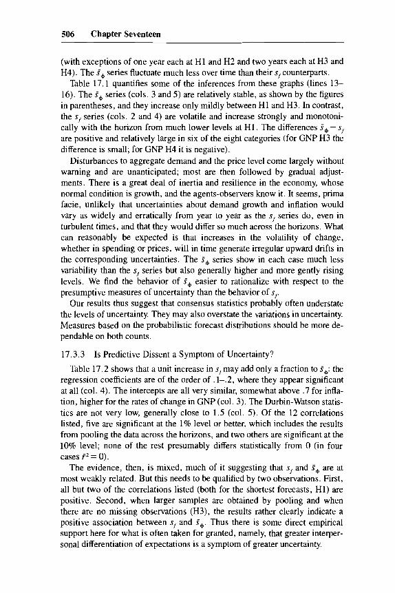
Table 17.2 shows that a unit increase in Sf may add only a fraction to s4>: theregression coefficients are of the order of .1-.2, where they appear significantat all (col. 4). The intercepts are all very similar, somewhat above .7 for infla­tion, higher for the rates of change in GNP (col. 3). The Durbin-Watson statis­tics are not very low, generally close to 1.5 (col. 5). Of the 12 correlationslisted, five are significant at the 1% level or better, which includes the resultsfrom pooling the data across the horizons, and two others are significant at the10% level; none of the rest presumably differs statistically from 0 (in fourcases f2 = 0).

The evidence, then, is mixed, much of it suggesting that sf and &4> are atmost weakly related. But this needs to be qualified by two observations. First,all but two of the correlations listed (both for the shortest forecasts, HI) arepositive. Second, when larger samples are obtained by pooling and whenthere are no missing observations (H3), the results rather clearly indicate apositive association between sf and s4>. Thus there is some direct empiricalsupport here for what is often taken for granted, namely, that greater interper­sonal differentiation of expectations is a symptom of greater uncertainty.

507 Consensus and Uncertainty in Economic Prediction

The reasons why this support is not stronger may lie in certain offsettingeffects. Thus one can argue that it is precisely when uncertainty is high thatpeople will have strong incentives to reduce the risk of making eccentric er­rors and will invest more resources in interactive prediction (see sec. 17.1.1).To the extent that this is true, it would tend to make the individual expecta­tions (point forecasts) more closely bunched at such times; that is, it wouldproduce elements of inverse correlation between Sf and 5<1>'

A warning is in order at this point. Our findings are based on small samplesof observations. Pooling the data can help but is no substitute for longer seriesof matching point and probabilistic forecasts. Collection and processing ofmore information of this type should in time produce more conclusive results.

17.3.4 Inflation Expectations and Uncertainty

Our data permit direct tests of the hypothesis that changes in anticipatedinflation tend to cause parallel changes in uncertainty about inflation. Thisidea plays an important role in theories that view rising (and high and volatile)inflation as a major source of adverse real effects (see sec. 17.1.3).

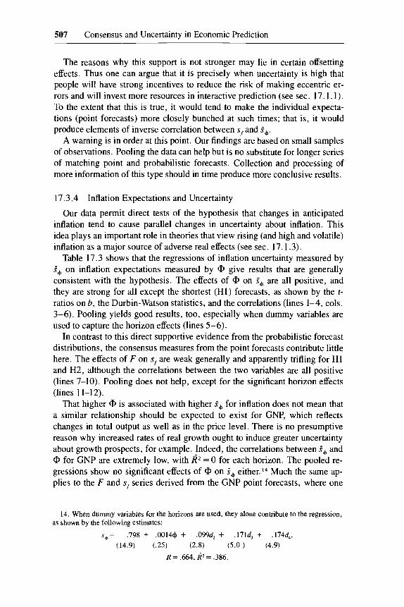
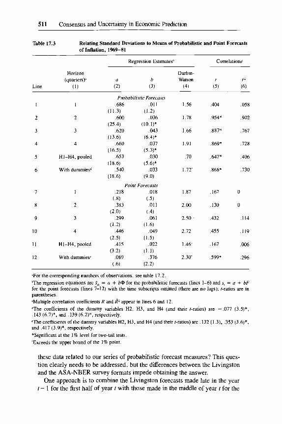
Table 17.3 shows that the regressions of inflation uncertainty measured by5<t> on inflation expectations measured by <I> give results that are generallyconsistent with the hypothesis. The effects of <I> on 5<1> are all positive, andthey are strong for all except the shortest (H1) forecasts, as shown by the t­ratios on b, the Durbin-Watson statistics, and the correlations (lines 1-4, cols.3-6). Pooling yields good results, too, especially when dummy variables areused to capture the horizon effects (lines 5-6).

In contrast to this direct supportive evidence from the probabilistic forecastdistributions, the consensus measures from the point forecasts contribute littlehere. The effects of F on Sf are weak generally and apparently trifling for HIand H2, although the correlations between the two variables are all positive(lines 7-10). Pooling does not help, except for the significant horizon effects(lines 11-12).

That higher <I> is associated with higher 5<t> for inflation does not mean thata similar relationship should be expected to exist for GNP, which reflectschanges in total output as well as in the price level. There is no presumptivereason why increased rates of real growth ought to induce greater uncertaintyabout growth prospects, for example. Indeed, the correlations between 5<t> and<I> for GNP are extremely low, with R2 = 0 for each horizon. The pooled re­gressions show no significant effects of <I> on 5<t> either. 14 Much the same ap­plies to the F and Sf series derived from the GNP point forecasts, where one

14. When dummy variables for the horizons are used, they alone contribute to the regression,as shown by the following estimates:

Set> = .798 + .OOI4<f> + .099dz + .171d3 + .174d4 ,

(14.9) (.25) (2.8) (5.0 ) (4.9)

R = .664, RZ = .386.

HO

RIZ

ON

1G

NP

HO

RIZ

ON

2G

NP

% 2.0.

i

% 2.0.

i

1.5

1.5

s.,,

'\\

....~:

"~..

\S

,/'

\.....

.~",,'

\/

/",

-.....

....

".-

.J..

....

."

1.0

0.5

s.--

----

----

----

----

--/~,

Sf---

------

----_

/"------

------

---

1.0

0.0'

11

1"i

11

•ii'

6970

7172

7374

7576

7778

7980

810

.0'

11"i

i'i

iii

1

6970

7172

7374

7576

7778

7980

81

HO

RIZ

ON

3G

NP

HO

RIZ

ON

4G

NP

% 2.0.

•% 2.0.

,

1.5

1.0

0.5

,,,,,,

,,"'-'

" /'\

/

1.5

1.0

0.5

-"""""

,..S

.""

,/

-

...---

----

'/

_'_'

__.

,I

Sf~

o.o~

,--

----~

6970

7172

7374

7576

7778

7980

810.

0 6970

7172

7374

7576

7778

7980

81

HO

RIZ

ON

2IP

D% 2.

0•

HO

RIZ

ON

1IP

D%

,2.

0

1.5

1.5

\ \.....

....."

'~f...

......

......

....

,

1.0

0.5

•_

_-----••-~-

til"_._

.-.

,

....

....

,I

"'-

"..."

I"

_"

,-_

_5

1-'

/".

~..,

1.0

0.5

.\-~

..------

---I

,,---,,-

----_.

10.

0··

··

··

··

··

··

·69

7071

7273

7475

7677

7879

8081

0.0·

,,

•,

,,

,,

,'

•.

6970

7172

7374

7576

7778

7980

81

HO

RIZ

ON

3IP

DH

OR

IZO

N4

IPD

% 2.0

'% 2.

0,

1.5

1.5

1.0

/'

1/

,I

0.5

P.,

/.....

..I

--""

....

,

1.0

0.5

_.....

.........

",,,

,--.

..J

'::•

•::-

----

~tIl~

.........._-~

"

~I

Sf\

I\,1

0.0·

,.

.,

..

..

..

..

6970

7172

7374

7576

7778

7980

810.

0.•

,•

•,

•,

,•

,,

,69

7071

7273

7475

7677

7879

8081

Fig

.17

.3S

tand

ard

devi

atio

nsan

dpr

obab

ilis

tic

fore

cast

sof

rate

sof

chan

gein

GN

Pan

dIP

D,

four

hori

zons

,an

nual

,19

69-8

1N

ote:

Lon

g-da

shed

line

sre

fer

tost

anda

rdde

viat

ions

of

poin

tfo

reca

sts

(sf)

;so

lid

line

sre

fer

tost

anda

rdde

viat

ions

of

prob

abil

isti

cfo

reca

sts

(sct

»;sh

ort-

dash

edli

nes

indi

cate

mis

sing

obse

rvat

ions

.

510 Chapter Seventeen

Table 17.2 Relating Time Series of Standard Deviations of Point and ProbabilisticForecasts, Annual Percentage Changes in GNP and IPD, 1969-81

Regression Estimatesa Correlationsb

Horizon No. of Durbin-(quarters) Observations a b Watson r f2

Line (1) (2) (3) (4) (5) (6) (7)

Gross National Product10 .885 -.118 2.08 - .237 0

(12.5) (- .7)2 2 12 .810 .157 1.64 .545** .226

(15.8) (2.0)**3 3 13 .753 .255 1.03 .758* .536

(12.1) (3.9)*4 4 11 .934 .044 1.48 .114 0

(6.3) (.3)5 HI-H4, pooled 46 .764 .209 1.48t .710* .493

(28.8) (6.7)*6 With dummiesc 46 .744 .168 1.59t .756* .530

(25.6) (3.6)*

Implicit Price Deflator7 10 .785 -.078 1.63 - .280 0

(21.2) (-.8)8 2 12 .774 .120 .79 .295 0

(12.6) (1.0)9 3 13 .772 .181 1.97 .534** .221

(11.9) (2.1)**10 4 11 .736 .179 1.27 .467 .131

(9.0) (1.6)11 HI-H4, pooled 46 .740 .182 1.59t .525* .259

(27.0) (4.1)*12 With dummiesd 46 .714 .131 1.56t .606* .306

(23.1) (2.6)*

aThe regression equations are 5<1> = a + bSf (with the time subscripts omitted; there are no lags); t-ratiosare in parentheses.

bMultiple correlation coefficients Rand R2 appear in lines 6 and 12.

(The coefficients of the dummy variables H2, H3, and H4 (and their t-ratios) are .059 (1.8)**, .086(2.2)***, and .049 (1.0), respectively.

*Significant at the 1% level for two-tail tests.

**Significant at the 10% level for two-tail tests.

***Significant at the 5% level for two-tail tests.

tExceeds the upper bound of the 1% point.

of the correlations is negative and only one (for H4) is positive and significantat the 10% level.

17.3.5 Cross-Survey Analysis

The literature discussed in section 17.1.3 makes extensive use of measuresbased on the point forecasts of inflation from the Livingston surveys. How are

511 Consensus and Uncertainty in Economic Prediction

Table 17.3 Relating Standard Deviations to Means of Probabilistic and Point Forecastsof Inflation, 1969-81

Regression Estimatesh CorrelationsC

Horizon Durbin-(quarters )a a b Watson r ;2

Line (1) (2) (3) (4) (5) (6)

Probabilistic Forecasts.686 .011 1.56 .404 .058

(11.3) (1.2)

2 2 .600 .036 1.78 .954* .902(25.4) (10.1)*

3 3 .620 .043 1.66 .887* .767(13.6) (6.4)*

4 4 .660 .037 1.91 .869* .728(16.5) (5.3)*

5 HI-H4, pooled .653 .030 .70 .647* .406(18.6) (5.6)*

6 With dummiesd .540 .033 1.72t .868* .730(18.6) (9.0)

Point Forecasts

7 .218 .018 1.87 .167 0(.8) (.5)

8 2 .383 .011 2.00 .130 0(2.0) (.4)

9 3 .299 .061 2.50 . .432 .114(1.2) (1.6)

10 4 .446 .049 2.72 .455 .119(2.5) (1.5)

II HI-H4, pooled .415 .022 1.46t .167 .006(3.2) (1.1)

12 With dummiese .089 .376 2.30t .599* .296(.6) (2.2)

aFor the corresponding numbers of observations, see table 17.2.

"The regression equations are set> = a + b<t> for the probabilistic forecasts (lines 1-6) and Sf = a + bFfor the point forecasts (lines 7-12) with the time subscripts omitted (there are no lags); t-ratios are inparentheses.

cMultiple correlation coefficients Rand R2 appear in lines 6 and 12.

dThe coefficients of the dummy variables H2, H3, and H4 (and their t-ratios) are - .077 (3.5)*,.143 (6.7)*, and .139 (6.2)*, respectively.

eThe coefficients of the dummy variables H2, H3, and H4 (and their t-ratios) are .132 (1.3), .353 (3.6)*,and .417 (3.9)*, respectively.

*Significant at the 1% level for two-tail tests.

tExceeds the upper bound of the I% point.

these data related to our series of probabilistic forecast measures? This ques­tion clearly needs to be addressed, but the differences between the Livingstonand the ASA-NBER survey formats impede obtaining the answer.

One approach is to combine the Livingston forecasts made late in the yeart - 1 for the first half of year t with those made in the middle of year t for the

512 Chapter Seventeen

second half. The resulting annual averages, called LIV6, are paired with themeans of the ASA-NBER forecasts with horizons H4 and H2 for year t, la­beled ANB6. The component predictions of LIV6 and ANB6 have similardates, 15 but the targets of the former are semiannual and those of the latter areannual. This complication is avoided by an alternative procedure, which is tomatch the projections for t from the late t - 1 surveys of Livingston and ASA­NBER H4 (we refer to these series as LIV12 and ANBI2).

For all these differences, plus the fact that the Livingston surveys aim at therate of change in consumer prices (CPI) while the ASA-NBER surveys aim atinflation in terms of the IPD, the mean forecasts for LIV6 and ANB6 and forLIV12 and ANB 12 are highly correlated, as demonstrated in table 17.4, lines1-2. Of course, these associations are not quite as close'as those between theF and <I> series within the ASA-NBER set.

More remarkable yet, the correlations between the Sf series for LIV and theS<t> series for ANB are rather high and significant at the level of 1% or less(lines 3 and 4). There is more evidence here that low (high) consensus indi­cates high (low) uncertainty than in the relationships between the Sf and S<t>

series within the ASA-NBER set as examined in table 17.2 and section17.2.3.

It is true that the significance of these results is difficult to assess, given thesmallness of the available data samples. Pooling cannot be used here to alle­viate the problem. The Durbin-Watson statistics are not very low, but the re­siduals from some of the regressions appear to be positively autocorrelated.

In the ANB series used in table 17.4, H3 figures are interpolated in theinstances in which H2 or H4 figures are not available. However, to guardagainst a possible bias from this procedure, alternative regressions were cal­culated discarding all observations for which the H2 or H4 forecasts are miss­ing. 16 The main results of this procedure for the equations sf= a + bS<f> are thefollowing: for LIV6-ANB6, b=5.600 (3.6); D-W=2.31, r=.784; forLIVI2-ANBI2, b = 3.988 (3.8); D-W = 2.34, r = .788 (t-ratios and r signif­icant at the 1% level in a two-tail test). Compared with their counterparts intable 17.4, the values of the t-ratios and r are lower here and the Durbin­Watson statistics much higher. The finding that the LIV Sf series are positivelyrelated to the ANB S<f> series remains intact, so the interpolations seem to havelittle to do with it. 17

15. The Livingston midyear and end-of-year surveys are taken about a month after the corre­sponding ASA-NBER surveys (see table 17.4, n. a).

16. This "classical least squares" method of dealing with the problem of missing observationsis used throughout elsewhere in this study.

17. There is also no evidence that the interpolations cause any serious distortions in the otherequations estimated in table 17.4. Without interpolations, the t-ratios of band r values are some­what higher in lines 1 and 2, somewhat lower in lines 5-8, but all are still significant at the levelof 1% or less. The Durbin-Watson statistics are generally higher, exceeding 2.3 in all but threecases, which suggests that the interpolations might have induced some autocorrelation in the resid­uals from the regressions of table 17.4.

513 Consensus and Uncertainty in Economic Prediction

Table 17.4 Relating the Uncertainty and Consensus Measures for the ASA-NBER andLivingston Inflation Forecasts, 1969-81

Regression Estimatesb Correlations

Durbin-Survey Dataa a b Watson r ;2

Line (1) (2) (3) (4) (5) (6)

Mean Forecasts (F, <f»

LIV6, ANB6 -.811 1.040 1.48 .937* .868( -1.0) (8.9)*

2 LIVI2, ANB12 - .553 1.024 1.56 .956* .906(-.9) (10.8)*

Standard Deviations (Sf' 54»

3 LIV6, ANB6 - 3.058 5.470 1.29 .849* .696

(-3.4) (5.3)*

4 LIVI2, ANB12 -1.854 3.480 1.50 .811 * .625( -2.7) (4.6)*

Standard Deviations on Mean Forecasts5 LIV6 (Sf' F) .426 .217 1.73 .898* .789

(2.1) (6.8)*

6 LIV12 (Sf' F) .280 .169 1. 78 .906* .804(1.9) (7.1)*

7 ANB6 (54)' <f» .615 .040 1.63 .954* .902(24.5) (10.6)*

8 ANB12 (54)' <f» .637 .041 1.17 .891* .774(15.3) (6.5)*

aLIV6 are annual F and Sf series for inflation (CPI) based on forecasts from surveys taken in Decemberof year t - 1 for the first half of year t and in June of t for the second half of t. LIV12 are correspondingseries based on December (t - 1) forecasts for year t. ANB6 are annual <f> and 54> series for inflation(lPD) based on forecasts taken in November of t - 1 and May of t for the year t. ANBI2 are correspond­ing series based on November (t - I) forecasts for year t.

bThe regression equations are of the form F = a + b<f> for lines 1-2, Sf '= a + b54> for lines 3-4,Sf = a + bF for lines 5-6, and 54> = a + b<l> for lines 7-8. The F and Sf series refer to LIV6 andLIVI2; the <I> and 54> series to ANB6 and ANB 12. t-ratios are in parentheses. The number of observationsis 13 in each regression (for one missing observation in the H2 series and two in the H4 series, thecorresponding values of H3 are interpolated).

*Significant at the 1% level for two-tail tests.

What probably does help explain these results is that they are based on 6­month and, to a larger extent, 12-month forecasts, omitting the shortest hori­zon for which the association between Sf and S<t> may be much weaker, as table17.2 would suggest. In any event, table 17.4 provides direct support for theuses of the Livingston IT series as a proxy measure of uncertainty. This seemsto be the first evidence of this kind, and as such it is both noteworthy andfavorable.

The last section of table 17.4 confirms that S<t> rises with <I> (cf. lines 7-8and table 17.3, lines 1-6), but it also shows that Sf rises with F for both theLIV6 and the LIV12 series (lines 5-6). The latter effects seem rather strong,

514 Chapter Seventeen

which contrasts sharply with the evidence of weak or no relationship betweenstand F in the ASA-NBER data (see table 17.3, lines 7-12).

Source: ANB: ASA-NBER surveys; LIV: Livingston surveys; DM, TBR, and DGE: Bureau of Eco­nomic Analysis Handbook o/Cyclical Indicators, 1984.

Note: t-statistics are in parentheses.

aDM is the annual rate of change in the money supply, M1 (%); TBR is the 3-month Treasury bill rate;DGE is the annual rate of change in the total of real federal government expenditures and real exports(%); for the ANB and LIV variables, see the text and table 17.4.

bThe dependent variable is the annual rate of change in real GNP (%) (DY).

515 Consensus and Uncertainty in Economic Prediction

tainty LIV12 sf are used instead of ANB 54> (cf. eqs. [5.1]-[5.2] with eqs.[5.3]-[5.4] ).

Reciprocal relations being ubiquitous in economics, the direction of causa­tion is often difficult to establish: surely a prime example of this is that DY canaffect DM as well as the other way around. But it makes good sense to arguethat uncertainty about future inflation can influence real activity adversely intimes of rapid and irregular rises in the price level (such as the 1970s),whereas the reverse causation is implausible here. (Why should low DY in­duce high o-?)

The t-ratios leave little doubt about the significance of the separate effectsof the DM and 0- variables, with a couple of possible exceptions that probablyreflect collinearity problems. 18 Jointly, these variables account for about .5-.7of the variance of DY, depending on whether their lagged terms are included(see the R2coefficients). Real defense and other federal government purchasesof goods and services are usually treated as an exogenous determinant of totaloutput of the economy, and the same applies to real exports. However, addingthe rate of change in real federal expenditures and exports (DGE) to regres­sions with current and lagged values of DM and 5<f> turned out to contributevery little or nothing. 19 The variable DGE t was somewhat more effective (butat some expense of DM t ) when used along with the sf series, as illustrated byequation (5.6). Also, there are some indications of a negative influence on DYof lagged interest rates (represented by the Treasury bill rate [TBR]), but theytoo are somewhat sporadic ,and weak (eq. [5.5]).20

In sum, the idea of inflation uncertainty as a short-term depressant of realactivity receives substantial support from table 17.5. The Livingston Sf dataprovide on the whole a good proxy measure of 0- in this context. These resultsare consistent with recent studies. 21 They seem sufficiently robust to meritcautious acceptance at this time, pending the accumulation of more evidence.

17.3.7 Effects on Interest Rates

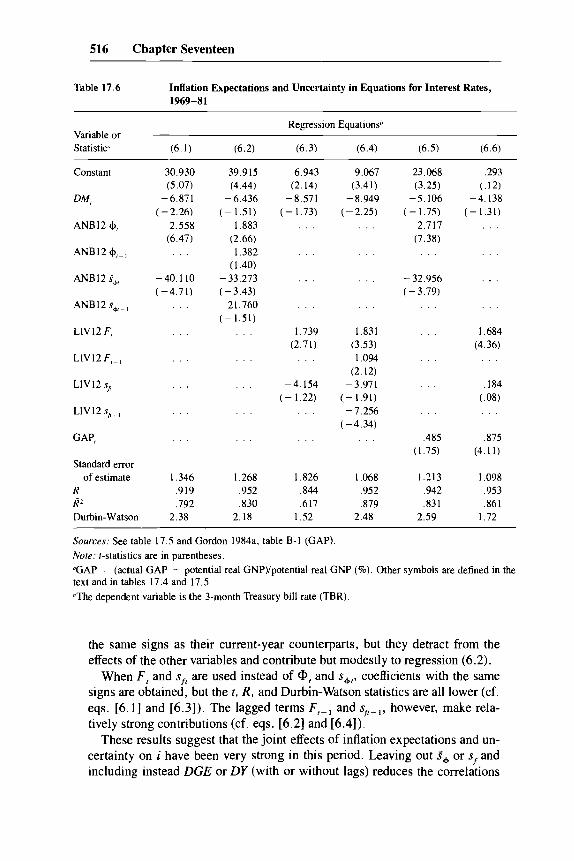
Interest rates (i) represented by TBR t depend positively on expected infla­tion <l>t and inversely on inflation uncertainty 54>t and money growth DMt, asseen in table 17.6, equation (6.1). The lagged terms <l>t-l and S4>t-l enter with

18. The addition of ANB12s4>t_l results in a low t for DMt_ 1 and reduces the Durbin-Watsonstatistics (which otherwise exceed 2). The addition of LIV12s/t_l results in a low t for DMt • Thecorrelations between s4>t and S4>t-l is .463, that between Sft and Sft-l is .618, and for DMt andDMt_ 1

the corresponding statistic is .410.19. That is, neither DY nor the coefficients of the other variables were significantly affected. We

have also tried, with similarly negative results, a series of shares of federal government purchasesand exports in GNP.

20. No further search for missing variables was considered necessary or indeed desirable, giventhe pitfalls of data mining and our limited objectives.

21. See Levi and Makin 1980 and Makin 1982. It should be noted that this refers only to therole of <t> t. Our calculations were not designed to deal with the issue of anticipated versus unantic­ipated money growth (me vs. mU

); their outcome is consistent either with me having real effects orwith mu accounting for the largest part of total monetary change.

the same signs as their current-year counterparts, but they detract from theeffects of the other variables and contribute but modestly to regression (6.2).

When Ft and S/t are used instead of <I> t and S 4>t' coefficients with the samesigns are obtained, but the t, R, and Durbin-Watson statistics are all lower (cf.eqs. [6.1] and [6.3]). The lagged terms Ft - 1 and Sjt-l' however, make rela­tively strong contributions (cf. eqs. [6.2] and [6.4]).

These results suggest that the joint effects of inflation expectations and un­certainty on i have been very strong in this period. Leaving out S4> or S j andincluding instead DGE or DY (with or without lags) reduces the correlations

517 Consensus and Uncertainty in Economic Prediction

greatly. The influence of DMt

- 1 turns out to be weak and ambiguous in itssign.

The evidence of equations (6.1)-(6.4) supports the proposition that infla­tion uncertainty (J' influences i negatively, which is consistent with three of therecent papers that use the Livingston Sf data for the same purpose. (Two othersreport positive and one reports insignificant coefficients for the current and/orlagged values of Sp see sec. 17.1.3.) A study by Lahiri, Teigland, and Zapo­rowski (1986), using s<P-type data from the ASA-NBER surveys, finds posi­tive effects that, however, are insignificant in the presence of selected "liquid­ity" and "exogenous demand" variables. 22

When the percentage divergence of actual from potential real GNP (GAP)is added to the equation with current and lagged values of the LIV measures,its impact on TRB is revealed as positive and strong. 23 The addition of GAP t

diminishes the effect of DM t and eliminates that of Sft (cf. eqs. [6.3] and[6.6]). That the impact of sf on TRB (as observed in earlier papers written orcoauthored by Makin) disappears when GAP is included has been noted byMakin and Tanzi (1984, pp. 130, 134). In contrast to Sf' however, S<P retainsits significantly large coefficient with a negative sign in the presence of GAP(cf. eqs. [6.2] and [6.5]).

The upshot is that the balance of the evidence, with more credence given tothe probabilistic than to the point forecast data, favors the view that the effectof a rise in (J' is to reduce i. As noted earlier, this implies that real investmentis depressed more than real savings in the process. However, this result needsto be treated with caution since it could be quite sensitive to the choice of thetime period covered and other specifications.

17.4 Conclusions

We define "consensus" as the degree of agreement among correspondingpoint predictions by different individuals and "uncertainty" as the diffusenessof the probability distributions attached by the same individuals to their pre­dictions. To be useful the distinction must be made operational and measur­able. The quarterly ASA-NBER surveys provide data on point and probabilis­tic forecasts of annual percentage changes in GNP and IPD, which can beapplied to this task in several ways.

22. The authors pool the survey data across horizons and combine them with quarterly seriesfor other variables. They use 3- and 6-month Treasury bill rates when the forecast horizon is twoquarters or less and 12-month rates when it is three quarters or more; the two situations are alsodistinguished by means of dummy variables. The period covered is 1969:2-1985:2. Thus theirstudy differs from ours in several respects, and it is not clear what accounts for the discrepancy inthe results.

23. GAP is a cyclical factor, which is a broad measure of capacity utilization that affects realinvestment positively via an accelerator-type relationship (see Tanzi 1980; Makin and Tanzi1984).

518 Chapter Seventeen

The matched mean point forecasts (F) and mean probability forecasts (<I»agree closely. On the whole, then, the preferred predictions coincide with theexpected values of the probability distributions assessed by the survey respon­dents.

Standard deviations of point forecasts (Sf) tend to understate uncertainty asmeasured by the means of standard deviations of predictive probability distri­butions (s4»' particularly for short horizons. The sf series show much greatervariability over time than the s 4> series, but the evidence suggests that thesemeasures of consensus and uncertainty are for the most part positively corre­lated.

The Sf series derived from the semiannual Livingston survey forecasts havebeen widely used in recent literature as proxies for "inflation uncertainty."This practice receives direct support from our finding of substantial positivecorrelations between annual versions of these data and roughly consistent s4>

series of inflation based on ASA-NBER survey forecasts. However, matchingthe data from the two surveys presents small-sample and other measurementproblems; hence the results of this analysis must be interpreted with particularcaution.

Strong positive effects of <I> on s4> for the rate of change in IPD (but not inGNP) provide evidence in favor of the hypothesis that expectations of higherinflation tend to generate greater uncertainty about inflation.

Real economic activity represented by the rate of change in constant-dollarGNP is adversely affected by a rise in inflation uncertainty measured by s4>'

allowing for the influence of monetary growth and exogenous demand. TheLivingston sf data produce similar results, in this study and others.

A rise in uncertainty about inflation, other things equal, can either reduceor increase interest rates, depending on whether it depresses real investmentmore than real savings or vice versa. Studies using the sf data have producedmixed results, interpreted accordingly. Our results indicate that a rise in s4> onthe average lowered the Treasury bill rate in the years 1969-81.