Available online at www.sciencedirect.com Journal of Financial Markets 15 (2012) 207–232 Buy-side trades and sell-side recommendations: Interactions and information content $ Jeffrey A. Busse, T. Clifton Green, Narasimhan Jegadeesh n Goizueta Business School, Emory University, 1300 Clifton Road, Atlanta, GA 30322, Unites States Available online 3 September 2011 Abstract We examine the performance of buy-side institutional investor trades and sell-side brokerage analyst stock recommendations, as well as their interactions. Buy-side trades follow sell-side analyst recommendations but not the other way around. While buy-side purchases significantly outperform their sales, the difference in performance is largely concentrated on the day of the transaction. Following recommendation changes, buy-side trades in the same direction as the recommendation change earn the same returns as trades in the opposite direction. Therefore, institutional investors do not exhibit special skills in discerning the quality of recommendations. & 2011 Elsevier B.V. All rights reserved. JEL classification: G14 Keywords: Analyst recommendations; Institutional trading 1. Introduction Timely and accurate dissemination of information is critical for capital markets to function efficiently. Not surprisingly, enormous resources are spent collecting and analyzing market and stock-specific information. The agents involved in these tasks could be compensated for their role, broadly, in two ways. Skilled information producers could set up mutual funds to actively invest in stocks and collect fees from their investors, or, www.elsevier.com/locate/finmar 1386-4181/$ - see front matter & 2011 Elsevier B.V. All rights reserved. doi:10.1016/j.finmar.2011.08.001 $ We would like to thank Eugene Kandel (the editor) and an anonymous referee for helpful comments and suggestions. We also thank Russell Jame and Kevin Tang for research assistance. n Corresponding author. E-mail addresses: [email protected] (J.A. Busse), [email protected] (T.C. Green), [email protected] (N. Jegadeesh).
Transcript
Available online at www.sciencedirect.com
Journal of Financial Markets 15 (2012) 207–232
1386-4181/$ -
doi:10.1016/j
$We wou
suggestions.nCorrespo
E-mail ad
Narasimhan_
www.elsevier.com/locate/finmar
Buy-side trades and sell-side recommendations:Interactions and information content$
Jeffrey A. Busse, T. Clifton Green, Narasimhan Jegadeeshn
Goizueta Business School, Emory University, 1300 Clifton Road, Atlanta, GA 30322, Unites States
Available online 3 September 2011
Abstract
We examine the performance of buy-side institutional investor trades and sell-side brokerage
analyst stock recommendations, as well as their interactions. Buy-side trades follow sell-side analyst
recommendations but not the other way around. While buy-side purchases significantly outperform
their sales, the difference in performance is largely concentrated on the day of the transaction.
Following recommendation changes, buy-side trades in the same direction as the recommendation
change earn the same returns as trades in the opposite direction. Therefore, institutional investors do
not exhibit special skills in discerning the quality of recommendations.
Timely and accurate dissemination of information is critical for capital markets tofunction efficiently. Not surprisingly, enormous resources are spent collecting andanalyzing market and stock-specific information. The agents involved in these tasks couldbe compensated for their role, broadly, in two ways. Skilled information producers couldset up mutual funds to actively invest in stocks and collect fees from their investors, or,
see front matter & 2011 Elsevier B.V. All rights reserved.
.finmar.2011.08.001
ld like to thank Eugene Kandel (the editor) and an anonymous referee for helpful comments and
We also thank Russell Jame and Kevin Tang for research assistance.
J.A. Busse et al. / Journal of Financial Markets 15 (2012) 207–232208
alternatively, they could sell their information to investors through research reports, astypically done by sell-side analysts in brokerage firms.In practice, however, active mutual funds and brokerage analysts who communicate
directly with investors coexist. Mutual funds reveal their information through their trades,and sell-side analysts reveal their investment opinion through recommendations. Besidesissuing recommendations, sell-side analysts also provide additional services such as helpinggenerate trade commissions for their employer or assisting with investment bankingactivities.Sell-side analysts’ multi-faceted role potentially exposes them to conflicts of interest.
Concerns about such conflicts led to close scrutiny of analysts’ activities, which resulted inthe 2003 Global Analyst Research Settlement between ten large brokerage houses and theSEC and state regulators, which curtailed their activities in the area of investment banking.While this settlement reduced their involvement in investment banking activities, otherpotential conflicts remain. For example, Irvine (2001, 2004) finds evidence that tradingcommissions are an important determinant for the types of information that are releasedby brokerage analysts. In addition, surveys of institutional investors indicate thatproviding management access to information is an important service offered by brokerageanalysts. As a result, the desire to stay in the good graces of firm management may colorthe opinions of brokerage firm analysts.Mutual funds do not face these types of conflicts of interest. Their fees depend on the
amount of assets under management, and investors choose funds based primarily on theirpast performance (Warther, 1995; Sirri and Tufano, 1998). Therefore, one might expect themutual fund set-up to be the optimal mechanism to deliver the value of stock research toinvestors in the presence of agency conflicts.We present a comparative analysis of the performance of stocks recommended by
brokerage analysts and stocks that are traded by mutual funds and investigate the relativeinformation content. Several papers in the literature present evidence of the stock-pickingskills of mutual funds (e.g., Daniel, Grinblatt, Titman, and Wermers, 1997; Chen,Jegadeesh, and Wermers, 2000; Wermers, 2000, 2004) and sell-side analysts (e.g., Womack,1996; Barber, Lehavy, McNichols, and Trueman, 2001; Jegadeesh, Kim, Krische, and Lee,2004; Jegadeesh and Kim, 2006). Our study is the first to investigate the relativeinformation content of active funds’ trades and brokerage recommendations using thesame sample of stocks and the same sample period.We also investigate the relation between sell-side analysts’ recommendations and mutual
fund trades, addressing several issues that have been of interest both in the academicliterature and in the popular media. Academic studies often suggest that institutions aresophisticated investors who can sort through recommendations potentially tainted byanalysts’ incentives. For instance, Malmendier and Shanthikumar (2007) argue thatinstitutions take into account the fact that sell-side analysts tilt their recommendationstowards buy ratings but individual investors trade naively and ‘‘follow recommendationsliterally.’’The media and many investors also share such perceptions. For instance, a New York
Times article asserts that ‘‘For years, Wall Street’s dirty little secret was that its researchwas devised expressly for two key constituencies: its institutional investors and itscorporate clients. If the individual investor wanted to join the party, well, caveat emptor.’’1
1The New York Times, December 23, 2002, ‘‘Can settlements actually level the playing field for investors?’’
J.A. Busse et al. / Journal of Financial Markets 15 (2012) 207–232 209
Recent reports that ‘‘analysts at Goldman sometimes shared with traders and key clientsshort-term trading tips that sometimes differed from the firm’s long-term research’’2 addsupport to such perceptions.
Other media reports suggest that institutional investors are able to see through anyinherent biases in sell-side recommendations due to conflicts of interest, although theserecommendations may mislead retail investors. For example, a Euromoney article aboutthe Global settlement reports that ‘‘The managers attribute all the fuss to the lack ofsophistication among retail investors, who were too witless or ill-informed to translate theWall Street language of buy, strong buy, and hold. They didn’t seem to realize, a commonargument goes, that you had to call analysts to get their private views, not merely readtheir reports.’’3
The relation between mutual fund trades and sell-side analysts’ recommendations will shedlight on whether institutional investors are indeed able to differentiate between goodrecommendations and bad recommendations, as well as if these investors are a ‘‘keyconstituency’’ for sell-side analysts. If mutual funds use analyst recommendations as an inputfor their trading decisions, then we expect fund trades to be correlated with the direction ofanalyst recommendations. Moreover, if institutional investors have special access to analysts’private views or if they have superior abilities to understand recommendations, then weexpect analyst recommendations that are accompanied by mutual fund trades in the samedirection to outperform those that are accompanied by trades in the opposite direction.
In related work, Malmendier and Shanthikumar (2007) examine whether small investors arenaı̈ve about analysts’ conflicts of interest when they make recommendations, and theycompare the patterns of large trades and small trades around recommendation revisions.Malmendier and Shanthikumar’s dataset does not report the identity of the trader. Thereforethey classify trades as those by institutions or individuals based on trade size, and theyattribute large trades to institutions and small trades to individuals. However, institutionstypically break up their trades into small orders, and hence trades that are classified asindividual trades may well be parts of a larger institutional trade. In contrast, we useinstitutional trade datasets from Plexus and Abel/Noser in which we know that the trades areexecuted by institutions, and we also know the direction (buy or sell) of each trade.
Goldstein, Irvine, Kandel, and Wiener (2009) also use the Abel/Noser dataset toexamine institutional trades around recommendations. They focus on whether trades byinstitutional clients of the brokerage that employs the analyst issuing recommendationsdiffer from those by other institutions. However, they do not examine the incrementalinformation content of institutional trades, nor do they investigate whether institutions areable to differentiate between good recommendations and bad recommendations. It iscritically important to investigate whether institutions are able to differentiate betweengood and bad recommendations to understand whether institutional investors have specialinsights that individual investors lack.
We find that sell-side analysts’ recommendations are informative, which is consistentwith earlier findings in the literature. Although mutual fund purchases significantlyoutperform their sales, the difference in performance is largely concentrated on the day of
2See ‘‘Regulators Examine Goldman’s Trade Tips,’’ August 25, 2009, http://online.wsj.com/article/
SB125115914476055403.html.3Euromoney.com, February 1, 2003, ‘‘Where is all the buy-side outrage?’’
J.A. Busse et al. / Journal of Financial Markets 15 (2012) 207–232210
the trade. In direct comparisons, we find that sell-side analysts’ recommendations showsuperior stock-selection skills compared with mutual fund trades.We also find that mutual funds tend to trade in the direction of recommendation
revisions.4 However, mutual fund trades are not incrementally informative. Specifically,the performance of analyst recommendations that are accompanied by mutual fund tradesin the same direction is the same as those accompanied by trades in the opposite direction.In related work, a recent paper by Irvine, Lipson, and Puckett (2007) finds that analysts
tip institutional investors before they initiate recommendations with Buy or Strong Buyratings. Initiations are relatively rare compared with the number of upgrades anddowngrades that analysts issue. We examine here whether institutional trading prior torecommendation revisions indicates that they were tipped about impending revisions.We find that institutions are not net buyers prior to upgrades, but they are net sellers
prior to upgrades. Therefore, contrary to the findings in Irvine, Lipson, and Puckett (2007)for initiations, analysts do not seem to be tipping investors prior to regular upgrades.However, we find that institutions are significant net sellers over the five-day period priorto downgrades.5 This finding indicates that analysts potentially tip their clients prior todowngrades but not for upgrades.When we compare the performance of analysts’ recommendations with mutual fund trades,
we have to account for the fact that sell-side analysts publicly announce their recommendations,while mutual fund trades are not public information. Therefore, the impact of recommendationswould be quickly incorporated in prices, whereas the value of the signals on which mutual fundsbase their trades would only be reflected in prices over time. Moreover, mutual funds have accessto sell-side analysts’ recommendations when they make their trades. We develop a model thatallows us to make direct comparisons of the relative information content of analystrecommendations and mutual fund trades that take these factors into account.The paper proceeds as follows. Section 2 describes the data on fund trades and analyst
recommendations. Section 3 examines the performance of trades and recommendations,and Section 4 investigates the empirical relations between them. Section 5 concludes.
2. Data
2.1. Institutional trading
We use institutional funds’ trades to evaluate their stock-selection skills. We obtaininstitutional trading data from two sources: the Plexus Group (now owned by InvestmentTechnology Group) and Abel/Noser Corporation.6 Both companies are consulting firmsthat help institutional investors monitor and manage their transaction costs. Their clientsinclude both pension-plan sponsors and money managers, and the databases identify eachclient by a numeric code.
4Recent work by Brown, Wei, and Wermers (2007) examines, using quarterly data, whether fund trades in the
same direction as revisions lead to price pressure. Our findings indicate that the frequency of fund trades and
revisions that occur in the same direction is fairly small.5Irvine, Lipson, and Puckett (2007) do not examine trading patterns prior to initiations with negative ratings
such as Sell or Strong Sell.6Keim and Madhavan (1995), Conrad, Johnson, and Wahal (2002), and Irvine, Lipson, and Puckett (2007) are
some of the papers that use Plexus data; Hu (2009), Goldstein, Irvine, Kandel, and Wiener (2009) are some of the
studies that use Abel/Noser data.
J.A. Busse et al. / Journal of Financial Markets 15 (2012) 207–232 211
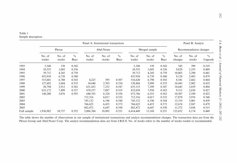
Table 1 presents a data summary. The Plexus sample covers the period from September1993 through December 2001. This dataset contains over 1.9 million transactions for10,737 different stocks. The Abel/Noser sample begins in 1997, ends in 2005, and containsabout 5.1 million transactions for 10,905 different stocks. Together, these two datasetscontain trades by 908 different institutional investors.7 About 55% of the trades are buys,and 45% are sells. The larger proportion of buys reflects the overall growth in assets undermanagement by institutions.
2.2. Analyst recommendations
We obtain analyst recommendations from the Institutional Brokers’ Estimate System(I/B/E/S) for the period from 1993 to 2005. The data consist of a ticker to identify therecommended stock, the date of the recommendation, the broker, and the analyst’srecommendation.8 I/B/E/S codes analyst recommendations using a 1–5 scale, with 1 signifyinga strong buy, 2 a buy, 3 a hold, 4 a sell, and 5 a strong sell. Analysts routinely change theirrecommendations based on any new information that they get, as well as on stock pricemovements relative to their target prices.
We follow the prior literature and use price changes following revisions in analysts’recommendations as a measure of the value of analysts’ information. Table 1 presentssummary statistics for our recommendation change sample over our 1993–2005 sampleperiod. There are about 55% downgrades and about 45% upgrades during this period.Overall, there are 135,652 recommendation revisions in the sample, covering 8,174different stocks.
We obtain individual stock returns, prices, volume of trades, shares outstanding, andexchange listings from the Daily and Monthly Stock files of the Center for Research inSecurity Prices (CRSP). Finally, we obtain financial statement data from Compustat. Weuse the CRSP and Compustat data to characterize the types of stocks that institutionstrade and analysts follow and to evaluate the performance of their stock picks.
3. Performance of institutional trades and recommendation changes
3.1. Institutional trades
We first evaluate the stock selection skills of analysts and funds. To measure skill, wecompute abnormal returns following trades and revisions on the event dates and forholding periods of one to four weeks and for two months and three months. Since analystspublicly announce their revisions, stock prices would react to the information content on
7When aggregating trading across institutions, we assume clients are unique across data providers, but the
results are not sensitive to this assumption. For the period when the samples overlap, we find similar results when
we use either source alone.8Recent work by Ljungqvist, Malloy, and Marston (2009) suggests that I/B/E/S has periodically modified its
database in non-random ways. Such modifications naturally can affect inference based on its historical record.
Ljungqvist, Malloy, and Marston (2009) indicate that many of the modifications have been reversed in recent
versions of the database. We base our analysis on a version of the database that appeared several months after
Ljungqvist, Malloy, and Marston (2009) indicate the issues were somewhat corrected. Furthermore, using
alternative databases such as Zacks and Thomson Financial’s First Call, numerous papers find evidence of price
patterns following analyst recommendations similar to our findings (e.g., Barber, Lehavy, and Trueman, 2007).
The table shows the number of observations in our sample of institutional transactions and analyst recommendation changes. The transaction data are from the
Plexus Group and Abel/Noser Corp. The analyst recommendation data are from I/B/E/S. No. of stocks refers to the number of stocks traded or recommended.
J.A
.B
usse
eta
l./
Jo
urn
al
of
Fin
an
cial
Ma
rkets
15
(2
01
2)
20
7–
23
2212
J.A. Busse et al. / Journal of Financial Markets 15 (2012) 207–232 213
the announcement date. However, funds do not publicly announce their trades. Therefore,any private information underlying their trades would be reflected in stock prices only overtime as the market learns that information through various channels.
In addition to computing raw returns over various holding periods, we also computeDGTW-adjusted abnormal returns because trades and revisions are tilted towards variouscharacteristics as Chen, Jegadeesh, and Wermers (2000) and Jegadeesh, Kim, Krische, andLee (2004) report. Similar to the findings in earlier studies, we find in unreported resultsthat both analysts and funds tilt their trades and revisions towards high momentum stocks,and funds exhibit a more significant momentum tilt than analysts. However, in our sample,we find that funds and analysts exhibit a preference for value stocks over growth stockswhile earlier studies report a preference for growth stocks.
We compute abnormal returns over various holding periods as:
ARi,tðHÞ ¼YtþH
t ¼ tð1þ ri,tÞ�
YtþH
t ¼ tð1þ rdgtw,tÞ, ð1Þ
where ri,t is the daily return for stock i, and rdgtw,t is the daily benchmark return from oneof 125 portfolios matched on size, book-to-market, and return momentum. H is the returnhorizon and varies from 0 to 62 days.
We take a transaction dollar-weighted mean of these returns within the month and thenaverage across months.9 We compute Fama and MacBeth (1973) standard errors, takinginto account autocorrelations over overlapping intervals for various holding periods, as inJegadeesh and Karceski (2009). Specifically, we compute standard errors allowing for first-order serial correlation for holding periods up to four weeks, up to second-order serialcorrelation for two-month holding periods, and up to third-order serial correlation forthree-month holding periods.
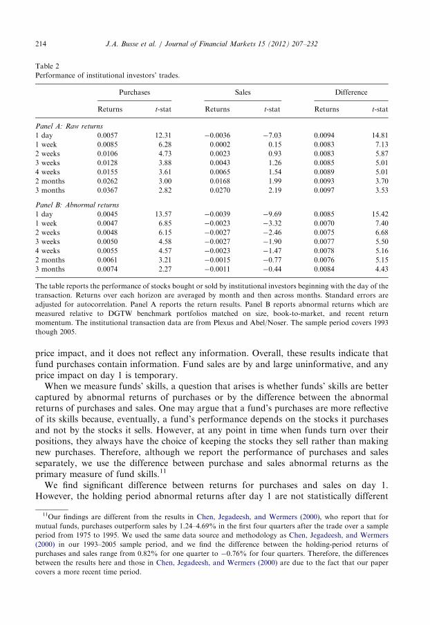
Table 2 reports the results for raw returns (Panel A) and DGTW-adjusted returns(Panels B, C, and D). Panels C and D examine large and small cap subsets respectively.The raw return results in Panel A show large transaction-day (‘‘one day’’) effects, withreturns on purchases of 0.57% and sales of �0.36%. Over time, the cumulative returns ofpurchases steadily increase, which, by itself, is not surprising, since the stock marketincreased during this sample period. Sales also show positive returns following the firstday.10 Consequently, the differences between purchases and sales in the last two columnsare the most relevant metrics for raw returns.
Panel B of Table 2 presents the DGTW-benchmark adjusted abnormal returns forinstitutional trades. The first day abnormal returns are positive for purchases (0.45%) andnegative for sales (�0.39%). The abnormal return difference is 0.85% on day 1. The pointestimates of abnormal return difference falls to 0.70% at the end of one week but increasesmarginally subsequently.
The pattern of change in abnormal returns over time is different for purchases and sales.In the case of purchases, abnormal returns increase from 0.45% on day 1 to 0.74% threemonths from the event date. Therefore, the price impact on day 1 reflects funds’information, and as time progresses, more of their information gets reflected in prices.However, in the case of sales, abnormal returns increase from �0.39% on day 1 to�0.11% at the end of three months. Therefore, the day 1 return for sales is a temporary
9Weighting the transactions equally within the month produces similar results.10We use the terminology ‘‘purchases’’ and ‘‘sales’’ to refer to institutional trades rather than the terms ‘‘buys’’
and ‘‘sells’’ to avoid any confusion with recommendation levels.
Table 2
Performance of institutional investors’ trades.
Purchases Sales Difference
Returns t-stat Returns t-stat Returns t-stat
Panel A: Raw returns
1 day 0.0057 12.31 �0.0036 �7.03 0.0094 14.81
1 week 0.0085 6.28 0.0002 0.15 0.0083 7.13
2 weeks 0.0106 4.73 0.0023 0.93 0.0083 5.87
3 weeks 0.0128 3.88 0.0043 1.26 0.0085 5.01
4 weeks 0.0155 3.61 0.0065 1.54 0.0089 5.01
2 months 0.0262 3.00 0.0168 1.99 0.0093 3.70
3 months 0.0367 2.82 0.0270 2.19 0.0097 3.53
Panel B: Abnormal returns
1 day 0.0045 13.57 �0.0039 �9.69 0.0085 15.42
1 week 0.0047 6.85 �0.0023 �3.32 0.0070 7.40
2 weeks 0.0048 6.15 �0.0027 �2.46 0.0075 6.68
3 weeks 0.0050 4.58 �0.0027 �1.90 0.0077 5.50
4 weeks 0.0055 4.57 �0.0023 �1.47 0.0078 5.16
2 months 0.0061 3.21 �0.0015 �0.77 0.0076 5.15
3 months 0.0074 2.27 �0.0011 �0.44 0.0084 4.43
The table reports the performance of stocks bought or sold by institutional investors beginning with the day of the
transaction. Returns over each horizon are averaged by month and then across months. Standard errors are
adjusted for autocorrelation. Panel A reports the return results. Panel B reports abnormal returns which are
measured relative to DGTW benchmark portfolios matched on size, book-to-market, and recent return
momentum. The institutional transaction data are from Plexus and Abel/Noser. The sample period covers 1993
though 2005.
J.A. Busse et al. / Journal of Financial Markets 15 (2012) 207–232214
price impact, and it does not reflect any information. Overall, these results indicate thatfund purchases contain information. Fund sales are by and large uninformative, and anyprice impact on day 1 is temporary.When we measure funds’ skills, a question that arises is whether funds’ skills are better
captured by abnormal returns of purchases or by the difference between the abnormalreturns of purchases and sales. One may argue that a fund’s purchases are more reflectiveof its skills because, eventually, a fund’s performance depends on the stocks it purchasesand not by the stocks it sells. However, at any point in time when funds turn over theirpositions, they always have the choice of keeping the stocks they sell rather than makingnew purchases. Therefore, although we report the performance of purchases and salesseparately, we use the difference between purchase and sales abnormal returns as theprimary measure of fund skills.11
We find significant difference between returns for purchases and sales on day 1.However, the holding period abnormal returns after day 1 are not statistically different
11Our findings are different from the results in Chen, Jegadeesh, and Wermers (2000), who report that for
mutual funds, purchases outperform sales by 1.24–4.69% in the first four quarters after the trade over a sample
period from 1975 to 1995. We used the same data source and methodology as Chen, Jegadeesh, and Wermers
(2000) in our 1993–2005 sample period, and we find the difference between the holding-period returns of
purchases and sales range from 0.82% for one quarter to �0.76% for four quarters. Therefore, the differences
between the results here and those in Chen, Jegadeesh, and Wermers (2000) are due to the fact that our paper
covers a more recent time period.
J.A. Busse et al. / Journal of Financial Markets 15 (2012) 207–232 215
from day 1 returns. In unreported tests, we also examine returns for up to one year afterthe trades and find no evidence of any drift. This finding is quite surprising since fundmanagers presumably trade based on their private information that is not reflected inmarket prices. However, any information that they may have is reflected in prices on theday they trade. Therefore, they do not seem to have any value-relevant information that isnot already reflected in prices on the day of the trade.
The evidence that the difference between abnormal returns on purchases and sales isalmost entirely due to the difference on the day of the trade indicates that price changesmay be due to the impact of their trades. The information content of trades depends onwhether the price impact is permanent or temporary. For instance, in Kyle’s (1985) model,trades convey the traders’ private information, and hence the accompanying price impactis permanent. However, price impact would be temporary if the trade is not informativeand the price eventually reverts to pre-trade levels. Thus, the pattern of returns in the dayssubsequent to a trade would reveal whether trades do indeed reveal funds’ value-relevantprivate information.
The abnormal returns over time in Table 2 indicate that the difference between purchaseand sales return remains at about the same level as on Day 1 over the next three months.12
For instance, the abnormal return difference on Day 1 is 0.85%, and it is 0.84% after threemonths. Therefore, the price change observed on the day of purchase and sales is permanent.
The evidence that the price impact is permanent indicates that the trades bring newinformation to the market. Our results indicate that the value of funds’ private informationis roughly 1%. A related issue is whether funds are able to fully profit from thisinformation. To investigate this issue, one should not only take into account the priceimpact but also all costs related to gathering the information and brokerage commissions.Our focus is on evaluating the information that funds bring to the market through theirtrades rather than the magnitude of their profits net of all costs.
It is possible that funds buy and sell stocks for a variety of reasons, and not all tradesmay be informationally motivated. For example, funds frequently experience inflows andoutflows from clients, and their trades to accommodate flows could be less informativethan trades motivated solely by their informational advantage. When funds trade toaccommodate flows, unless they have specific information about particular stocks, they arelikely to spread their trades across multiple stocks and trade relatively small quantities ofeach stock. However, if funds attempt to exploit their informational advantage aboutspecific stocks, they are likely to trade larger quantities of those stocks. More generally, thesize of fund trades would be determined by the perceived strength of funds’ information.We investigate whether funds’ informational advantage is more evident in their largertrades by partitioning trades into large and small trade subsamples. Specifically, we groupaggregate net order flow into two groups based on whether the absolute net order flow isabove or below the median calculated within each NYSE market capitalization decile overthe previous calendar year.
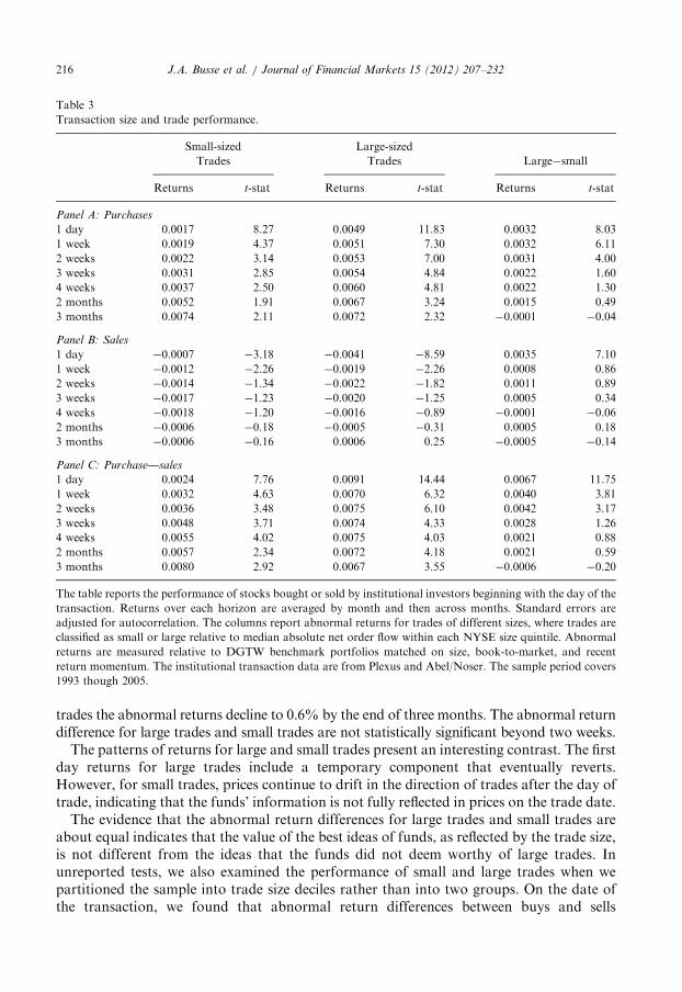
Table 3 reports abnormal returns for small and large trades. On the trade date, theabnormal return differences for small and large trades are 0.24% and 0.91%, respectively.The difference between these abnormal returns is statistically significant, indicating that largetrades convey more information to the market. For small trades, the abnormal returndifference continues to increase to 0.8% by the end of three months. However, for large
12In unreported tests, we find no evidence of any return reversals up to six months.
Table 3
Transaction size and trade performance.
Small-sized Large-sized
Trades Trades Large�small
Returns t-stat Returns t-stat Returns t-stat
Panel A: Purchases
1 day 0.0017 8.27 0.0049 11.83 0.0032 8.03
1 week 0.0019 4.37 0.0051 7.30 0.0032 6.11
2 weeks 0.0022 3.14 0.0053 7.00 0.0031 4.00
3 weeks 0.0031 2.85 0.0054 4.84 0.0022 1.60
4 weeks 0.0037 2.50 0.0060 4.81 0.0022 1.30
2 months 0.0052 1.91 0.0067 3.24 0.0015 0.49
3 months 0.0074 2.11 0.0072 2.32 �0.0001 �0.04
Panel B: Sales
1 day �0.0007 �3.18 �0.0041 �8.59 0.0035 7.10
1 week �0.0012 �2.26 �0.0019 �2.26 0.0008 0.86
2 weeks �0.0014 �1.34 �0.0022 �1.82 0.0011 0.89
3 weeks �0.0017 �1.23 �0.0020 �1.25 0.0005 0.34
4 weeks �0.0018 �1.20 �0.0016 �0.89 �0.0001 �0.06
2 months �0.0006 �0.18 �0.0005 �0.31 0.0005 0.18
3 months �0.0006 �0.16 0.0006 0.25 �0.0005 �0.14
Panel C: Purchase—sales
1 day 0.0024 7.76 0.0091 14.44 0.0067 11.75
1 week 0.0032 4.63 0.0070 6.32 0.0040 3.81
2 weeks 0.0036 3.48 0.0075 6.10 0.0042 3.17
3 weeks 0.0048 3.71 0.0074 4.33 0.0028 1.26
4 weeks 0.0055 4.02 0.0075 4.03 0.0021 0.88
2 months 0.0057 2.34 0.0072 4.18 0.0021 0.59
3 months 0.0080 2.92 0.0067 3.55 �0.0006 �0.20
The table reports the performance of stocks bought or sold by institutional investors beginning with the day of the
transaction. Returns over each horizon are averaged by month and then across months. Standard errors are
adjusted for autocorrelation. The columns report abnormal returns for trades of different sizes, where trades are
classified as small or large relative to median absolute net order flow within each NYSE size quintile. Abnormal
returns are measured relative to DGTW benchmark portfolios matched on size, book-to-market, and recent
return momentum. The institutional transaction data are from Plexus and Abel/Noser. The sample period covers
1993 though 2005.
J.A. Busse et al. / Journal of Financial Markets 15 (2012) 207–232216
trades the abnormal returns decline to 0.6% by the end of three months. The abnormal returndifference for large trades and small trades are not statistically significant beyond two weeks.The patterns of returns for large and small trades present an interesting contrast. The first
day returns for large trades include a temporary component that eventually reverts.However, for small trades, prices continue to drift in the direction of trades after the day oftrade, indicating that the funds’ information is not fully reflected in prices on the trade date.The evidence that the abnormal return differences for large trades and small trades are
about equal indicates that the value of the best ideas of funds, as reflected by the trade size,is not different from the ideas that the funds did not deem worthy of large trades. Inunreported tests, we also examined the performance of small and large trades when wepartitioned the sample into trade size deciles rather than into two groups. On the date ofthe transaction, we found that abnormal return differences between buys and sells
J.A. Busse et al. / Journal of Financial Markets 15 (2012) 207–232 217
generally increased with trade size (e.g., 0.21% for decile 1, 0.24% for decile 2, up to 1.35%for decile 10). However, the abnormal return differences were not meaningfully differentacross deciles beyond one month, with the exception of small return differences for decile 1.For example, the abnormal return difference after three months was 0.18% for decile 1compared to 0.80% and 0.75% for deciles 2 and 10, respectively. Perhaps the smallesttrades are uninformative because they are driven primarily by fund flows or diversificationmotives. Nevertheless, the important finding from our analysis here is that the value offunds’ information for even their best ideas as reflected by their trade size is about 1%.
It is possible that funds of different sizes exhibit different levels of stock selection skill.For instance, large funds may have the benefit of their own skilled analysts, but smallfunds may rely relatively more on outside sources. Our next set of tests examines therelation between stock selection skill and fund size. Our dataset does not directly reportfund size, and it only identifies funds by ID numbers and not by name. We determine theannual dollar trade volume for each fund and use this measure as a proxy for fund size.
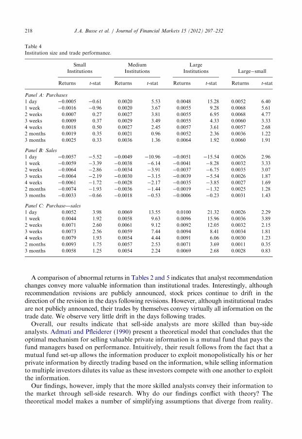
Table 4 presents abnormal returns for funds categorized based on size. We assign fundsto small, medium, and large categories based on their trading volume. Each year we sortinstitutions into three equal groups based on their total dollar trading volume. We then examineeach group’s trading activity over the following year. The difference in abnormal return forpurchases less sales on the trade date is monotonically related to fund size (0.52%, 0.69%, and1.00%), and the results for large funds are significantly different than small- and medium-sizedfunds. However, the abnormal return differences for the three categories converge over time. Bythe end of three months, the point estimates of abnormal return differences are roughly the samefor all three categories, and they are not statistically different. Therefore, the differences weobserve on the trade date are related to differences in price pressure across trades that aretemporary and not to differences in information content across funds of different sizes.Therefore, there is no evidence that funds of different sizes exhibit different levels of skill.
3.2. Analyst recommendations
We next examine the performance of stocks recommended by analysts. In particular, wefocus on the performance of stocks recently upgraded or downgraded. Table 4 presents theperformance of recommendation revisions. Panel A reports raw returns, and Panel Breports returns net of their DGTW benchmark.
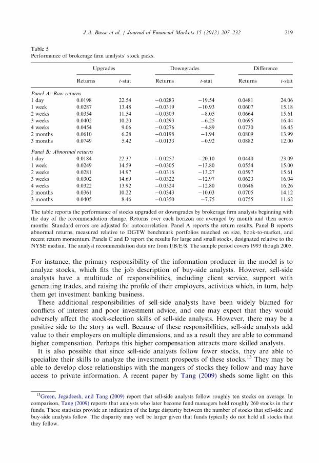
The stock price reaction for recommendation revision dates is much stronger than thestock price reaction for trade dates in Table 2. For instance, the average abnormal returnson upgrades and downgrades are 1.98% and �2.83%, compared with 0.64% and �0.54%for purchases and sales, respectively. This result per se is not surprising, since analystspublicly announce their recommendations, leading to a large announcement effect,whereas institutions seek secrecy to minimize the impact of their trades on prices.
Upgrades and downgrades continue to drift in the direction of revisions over the nextthree months. For example, the abnormal returns for upgrades increase to 4.05% andthose of the downgrades decline to �3.50% by the end of month 3. The differences in thelast set of columns in Table 2 show a large one-day effect followed by additional gainsthrough three months, though much of the total cumulative return occurs during the firstmonth (6.46% after four weeks and 7.55% after three months). The performance followingrecommendation changes is generally consistent with the literature on the value ofanalysts’ recommendation (e.g., Womack, 1996; Green, 2006).
J.A. Busse et al. / Journal of Financial Markets 15 (2012) 207–232218
A comparison of abnormal returns in Tables 2 and 5 indicates that analyst recommendationchanges convey more valuable information than institutional trades. Interestingly, althoughrecommendation revisions are publicly announced, stock prices continue to drift in thedirection of the revision in the days following revisions. However, although institutional tradesare not publicly announced, their trades by themselves convey virtually all information on thetrade date. We observe very little drift in the days following trades.Overall, our results indicate that sell-side analysts are more skilled than buy-side
analysts. Admati and Pfleiderer (1990) present a theoretical model that concludes that theoptimal mechanism for selling valuable private information is a mutual fund that pays thefund managers based on performance. Intuitively, their result follows from the fact that amutual fund set-up allows the information producer to exploit monopolistically his or herprivate information by directly trading based on the information, while selling informationto multiple investors dilutes its value as these investors compete with one another to exploitthe information.Our findings, however, imply that the more skilled analysts convey their information to
the market through sell-side research. Why do our findings conflict with theory? Thetheoretical model makes a number of simplifying assumptions that diverge from reality.
Table 5
Performance of brokerage firm analysts’ stock picks.
Upgrades Downgrades Difference
Returns t-stat Returns t-stat Returns t-stat
Panel A: Raw returns
1 day 0.0198 22.54 �0.0283 �19.54 0.0481 24.06
1 week 0.0287 13.48 �0.0319 �10.93 0.0607 15.18
2 weeks 0.0354 11.54 �0.0309 �8.05 0.0664 15.61
3 weeks 0.0402 10.20 �0.0293 �6.25 0.0695 16.44
4 weeks 0.0454 9.06 �0.0276 �4.89 0.0730 16.45
2 months 0.0610 6.28 �0.0198 �1.94 0.0809 13.99
3 months 0.0749 5.42 �0.0133 �0.92 0.0882 12.00
Panel B: Abnormal returns
1 day 0.0184 22.37 �0.0257 �20.10 0.0440 23.09
1 week 0.0249 14.59 �0.0305 �13.80 0.0554 15.00
2 weeks 0.0281 14.97 �0.0316 �13.27 0.0597 15.61
3 weeks 0.0302 14.69 �0.0322 �12.97 0.0623 16.04
4 weeks 0.0322 13.92 �0.0324 �12.80 0.0646 16.26
2 months 0.0361 10.22 �0.0343 �10.03 0.0705 14.12
3 months 0.0405 8.46 �0.0350 �7.75 0.0755 11.62
The table reports the performance of stocks upgraded or downgrades by brokerage firm analysts beginning with
the day of the recommendation change. Returns over each horizon are averaged by month and then across
months. Standard errors are adjusted for autocorrelation. Panel A reports the return results. Panel B reports
abnormal returns, measured relative to DGTW benchmark portfolios matched on size, book-to-market, and
recent return momentum. Panels C and D report the results for large and small stocks, designated relative to the
NYSE median. The analyst recommendation data are from I/B/E/S. The sample period covers 1993 though 2005.
J.A. Busse et al. / Journal of Financial Markets 15 (2012) 207–232 219
For instance, the primary responsibility of the information producer in the model is toanalyze stocks, which fits the job description of buy-side analysts. However, sell-sideanalysts have a multitude of responsibilities, including client service, support withgenerating trades, and raising the profile of their employers, activities which, in turn, helpthem get investment banking business.
These additional responsibilities of sell-side analysts have been widely blamed forconflicts of interest and poor investment advice, and one may expect that they wouldadversely affect the stock-selection skills of sell-side analysts. However, there may be apositive side to the story as well. Because of these responsibilities, sell-side analysts addvalue to their employers on multiple dimensions, and as a result they are able to commandhigher compensation. Perhaps this higher compensation attracts more skilled analysts.
It is also possible that since sell-side analysts follow fewer stocks, they are able tospecialize their skills to analyze the investment prospects of these stocks.13 They may beable to develop close relationships with the mangers of stocks they follow and may haveaccess to private information. A recent paper by Tang (2009) sheds some light on this
13Green, Jegadeesh, and Tang (2009) report that sell-side analysts follow roughly ten stocks on average. In
comparison, Tang (2009) reports that analysts who later become fund managers hold roughly 260 stocks in their
funds. These statistics provide an indication of the large disparity between the number of stocks that sell-side and
buy-side analysts follow. The disparity may well be larger given that funds typically do not hold all stocks that
they follow.
J.A. Busse et al. / Journal of Financial Markets 15 (2012) 207–232220
possibility. Tang examines the holdings of a sample of sell-side analysts who switched tothe buy side and finds that their holdings of stocks that they used to follow significantlyoutperform the market, but their other holdings do not. His findings provide support forthe idea that specialization helps.
4. Institutional trades and recommendation revisions—interactions
Since many institutions pay brokerages soft dollar commissions for their research, it isquite likely that they use their recommendations as inputs for their trading decisions.Additionally, it is also possible that analysts become aware of their clients’ trades after theyare executed and may use the information in trades as inputs for their recommendations.This section examines the interactions between institutional trades using recommendationrevisions. The first set of tests examines the lead-lag relation between trades and revisions.The second set of tests examines whether institutional trades are able to differentiatebetween more- and less-informative recommendation revisions.
4.1. Institutional trades and recommendation revisions—lead-lag relation
Analysts announce their recommendations revisions publicly, and the information isimmediately available both to the brokerages’ customers, as well as to subscribers ofvarious information providers. Thus, analyst recommendations are typically available toinstitutions when they make their trades. The converse is not necessarily true becauseinstitutions generally do not disclose their individual trades. However, analysts are likelyto be aware of institutional clients’ general interest in particular trades because funds oftencontact sell-side analysts for information about stocks that they actively evaluate. Also,when information flows from analysts flow to brokerage clients through events such as theGoldman Huddle, it is possible that information about clients’ trades flow to analystsas well.To investigate the interactions between institutional trades and analyst recommenda-
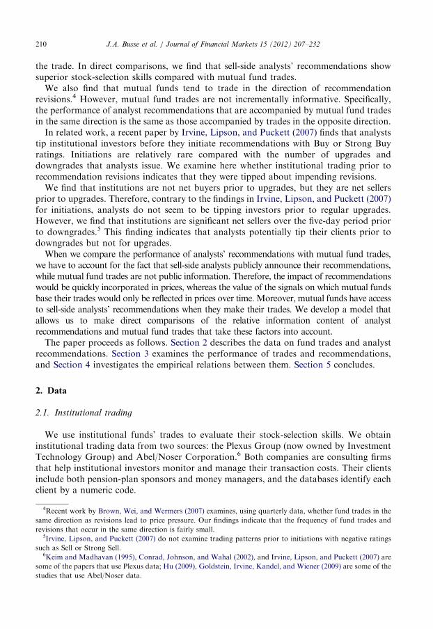
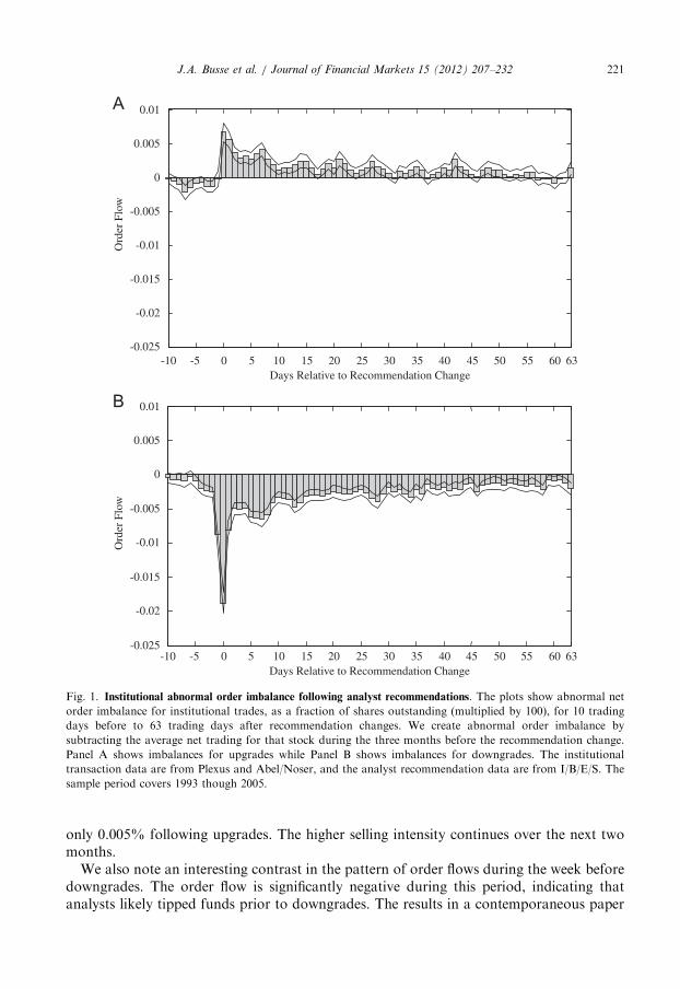
tions, we first examine the pattern of trades around recommendation revisions. Fig. 1presents daily abnormal order flows from 10 trading days before to 63 trading days afterrecommendation changes. We create abnormal order imbalance by subtracting the averagenet trading for that stock during the three-month period prior to the recommendationchange (trading days �73 to �11).14 The bars in the figure denote abnormal order flows,and the lines denote confidence intervals that are two-standard errors away from the meanestimates. Standard errors are computed using the cross-section of abnormal order flows ateach date.For upgrades, the order flow significantly increases on the day of recommendation
revisions. The order flow remains significant over the next 30 days. Interestingly, orderflows are negative in the days preceding an upgrade. Therefore, there is no evidence thatanalysts tip funds ahead of upgrades.The order flows are negative following downgrades, and the order flows remain
significantly negative for the next two months. Funds sell with a much greater intensityfollowing downgrades than they buy following upgrades. For example, funds in our samplesell �0.02% of the shares outstanding on the day of downgrades, and in comparison buy
14Using a six-month interval (126 trading days) for the benchmark period produces similar results.
Fig. 1. Institutional abnormal order imbalance following analyst recommendations. The plots show abnormal net
order imbalance for institutional trades, as a fraction of shares outstanding (multiplied by 100), for 10 trading
days before to 63 trading days after recommendation changes. We create abnormal order imbalance by
subtracting the average net trading for that stock during the three months before the recommendation change.
Panel A shows imbalances for upgrades while Panel B shows imbalances for downgrades. The institutional
transaction data are from Plexus and Abel/Noser, and the analyst recommendation data are from I/B/E/S. The
sample period covers 1993 though 2005.
J.A. Busse et al. / Journal of Financial Markets 15 (2012) 207–232 221
only 0.005% following upgrades. The higher selling intensity continues over the next twomonths.
We also note an interesting contrast in the pattern of order flows during the week beforedowngrades. The order flow is significantly negative during this period, indicating thatanalysts likely tipped funds prior to downgrades. The results in a contemporaneous paper
J.A. Busse et al. / Journal of Financial Markets 15 (2012) 207–232222
by Juergens and Lindsey (2009) are consistent with our findings. Juergens and Lindsey findthat sell volume through brokerages whose analysts downgrade a particular stock aresignificantly larger than that through other brokerages on days �2 and �1 relative to thedowngrade date. They do not find any significant increase in buy volumes prior toupgrades, which is consistent with our results. While Juergens and Lindsey examine tradingvolume through brokerages that employ the analysts and other brokerages, we directlyexamine the trades of institutional investors and find evidence of information leakage priorto downgrades.One potential explanation for the observation that analysts tip funds prior to
downgrades but not upgrades is that funds attach asymmetric values to obtaininginformation prior to recommendation changes. In the event of downgrades, funds wouldincur losses on their current holdings. Funds may therefore feel that they are caughtunawares if their broker does not warn them about impending downgrades. On the otherhand, a lack of warning prior to upgrades represents potential opportunity losses that maynot be resented by these funds.The pattern of order flows following recommendation revisions indicates that funds
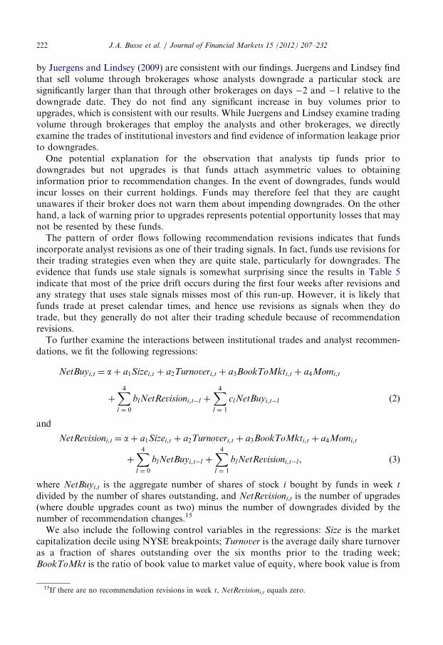
incorporate analyst revisions as one of their trading signals. In fact, funds use revisions fortheir trading strategies even when they are quite stale, particularly for downgrades. Theevidence that funds use stale signals is somewhat surprising since the results in Table 5indicate that most of the price drift occurs during the first four weeks after revisions andany strategy that uses stale signals misses most of this run-up. However, it is likely thatfunds trade at preset calendar times, and hence use revisions as signals when they dotrade, but they generally do not alter their trading schedule because of recommendationrevisions.To further examine the interactions between institutional trades and analyst recommen-
where NetBuyi,t is the aggregate number of shares of stock i bought by funds in week t
divided by the number of shares outstanding, and NetRevisioni,t is the number of upgrades(where double upgrades count as two) minus the number of downgrades divided by thenumber of recommendation changes.15
We also include the following control variables in the regressions: Size is the marketcapitalization decile using NYSE breakpoints; Turnover is the average daily share turnoveras a fraction of shares outstanding over the six months prior to the trading week;BookToMkt is the ratio of book value to market value of equity, where book value is from
15If there are no recommendation revisions in week t, NetRevisioni,t equals zero.
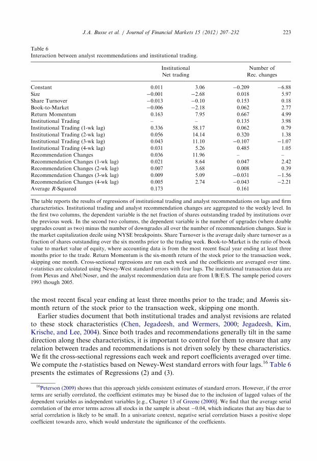
Table 6
Interaction between analyst recommendations and institutional trading.
The table reports the results of regressions of institutional trading and analyst recommendations on lags and firm
characteristics. Institutional trading and analyst recommendation changes are aggregated to the weekly level. In
the first two columns, the dependent variable is the net fraction of shares outstanding traded by institutions over
the previous week. In the second two columns, the dependent variable is the number of upgrades (where double
upgrades count as two) minus the number of downgrades all over the number of recommendation changes. Size is
the market capitalization decile using NYSE breakpoints. Share Turnover is the average daily share turnover as a
fraction of shares outstanding over the six months prior to the trading week. Book-to-Market is the ratio of book
value to market value of equity, where accounting data is from the most recent fiscal year ending at least three
months prior to the trade. Return Momentum is the six-month return of the stock prior to the transaction week,
skipping one month. Cross-sectional regressions are run each week and the coefficients are averaged over time.
t-statistics are calculated using Newey-West standard errors with four lags. The institutional transaction data are
from Plexus and Abel/Noser, and the analyst recommendation data are from I/B/E/S. The sample period covers
1993 though 2005.
J.A. Busse et al. / Journal of Financial Markets 15 (2012) 207–232 223
the most recent fiscal year ending at least three months prior to the trade; and Momis six-month return of the stock prior to the transaction week, skipping one month.
Earlier studies document that both institutional trades and analyst revisions are relatedto these stock characteristics (Chen, Jegadeesh, and Wermers, 2000; Jegadeesh, Kim,Krische, and Lee, 2004). Since both trades and recommendations generally tilt in the samedirection along these characteristics, it is important to control for them to ensure that anyrelation between trades and recommendations is not driven solely by these characteristics.We fit the cross-sectional regressions each week and report coefficients averaged over time.We compute the t-statistics based on Newey-West standard errors with four lags.16 Table 6presents the estimates of Regressions (2) and (3).
16Peterson (2009) shows that this approach yields consistent estimates of standard errors. However, if the error
terms are serially correlated, the coefficient estimates may be biased due to the inclusion of lagged values of the
dependent variables as independent variables [e.g., Chapter 13 of Greene (2000)]. We find that the average serial
correlation of the error terms across all stocks in the sample is about �0.04, which indicates that any bias due to
serial correlation is likely to be small. In a univariate context, negative serial correlation biases a positive slope
coefficient towards zero, which would understate the significance of the coefficients.
J.A. Busse et al. / Journal of Financial Markets 15 (2012) 207–232224
The results in Table 6 indicate that institutional trades are significantly related to tradesin the prior four weeks. The slope coefficients gradually decline from 0.336 for one-weeklagged trades to 0.031 for four-week lagged trades.17 Our findings indicate that wheninstitutions are net buyers of a stock in one week, then they are also on average net buyersof that stock over the next four weeks. This result is consistent with the findings ofinstitutional herding in Sias (2004).We also find that institutional trades are significantly correlated with contemporaneous
as well as lagged recommendation revisions. On the other hand, when fitting Regression(3), we find recommendation revisions are not correlated with lagged trades. There are twopossible interpretations of the correlation between trades and revisions. First, it is possiblethat institutions use recommendation revisions in their trading decisions, and vice versa.Alternatively, it is possible that both revisions and trades reflect common information, butthere is no causal relation between them.The result that both trades and revisions are positively related contemporaneously
suggests that the relation may be driven by common information, rather than by any causaleffect. For instance, both revisions and trades may be triggered by earnings announce-ments.18 However, in the case of lagged variables, trades are related to past revisions butnot the other way around. Taken together, the findings do not support the commoninformation hypothesis. It appears likely that at least some institutions use recommendationrevisions in their trading decisions.
4.2. Do trades differentiate between good and bad recommendations?
As we discuss in the Introduction, the academic literature and the popular press claim thatanalysts’ recommendations are tainted by conflicts of interest. Media reports and papers byMalmendier and Shanthikumar (2007) and others suggest that, while individual investors areapparently fooled, institutional investors can either see through biases in recommendations orthey have special access to analysts’ private views. This view implies that institutionsselectively use only the good recommendations and ignore the bad recommendations. Underthis hypothesis, upgrades that institutions purchase should outperform upgrades they sell,and downgrades that institutions purchase should outperform downgrades they sell as well.We examine the ability of institutions to differentiate between good and bad analyst
recommendations as follows. For each institutional trade observation, we examine whetherany analyst changed his recommendation for that stock within the preceding week. If therewere no recommendation changes in the preceding week, we discard the observation. Wethen compare the performance of recommendation revisions when institutions trade in thesame direction as revisions with those cases in which institutions trade in the oppositedirection.In Table 6, Panels A and B report the upgrade results. Panel A examines raw returns
while Panel B examines abnormal returns (returns net of the DGTW benchmark). The firsttwo columns of Panel A report the performance of institutional purchases. The patternevident in Panel A is similar to the analyst upgrade results in Table 4 and consistent withanalyst skill in upgrading stocks. The returns are positive and significant for most horizons.
17In unreported results, we find that the slope coefficients on institutional trades lagged five weeks or more were
not reliably different from zero.18We find similar results after excluding earnings announcement dates from the sample.
J.A. Busse et al. / Journal of Financial Markets 15 (2012) 207–232 225
The returns here are somewhat smaller than in Table 4, however, because Table 4 measuresreturns beginning the day of the recommendation change, while the results here exclude pricechanges up to one week from the date of upgrade. The next two columns, which report theresults for stocks upgraded but sold by institutions, show a less dramatic pattern with positiveand, in most cases, statistically significant returns. The last set of columns in Panel A reportsthe performance difference between purchases and sales. At the one-week horizon, purchasessignificantly outperform sales by 1.29%. This difference diminishes over the following weeksand is statistically insignificant at the three-month horizon. Panel B reports the abnormalreturn results, which are generally similar to the results in Panel A.
In Table 6, Panel C (raw returns) and Panel D (abnormal returns) report the downgraderesults. Similar to Panels A and B, the return pattern here differs from the downgradereturn pattern in Table 4 because we miss up to one week of the return following thedowngrade. Again, institutional purchases outperform their sales, but the performance islargely concentrated on the day of the trade.
At first glance, abnormal return differences between fund purchases and sales may seemto suggest that funds are able to differentiate between good and bad revisions. However, theentire return difference occurs on the day of trade. As Table 2 reports, fund purchases alsooutperform fund sales on the day of trade even without conditioning on recommendationrevisions on the trade date. Therefore, if funds are able to differentiate between goodrecommendations and bad recommendations, we would expect purchases to outperformsales around revisions by a larger magnitude than unconditionally.
The unconditional abnormal return difference on day 0 between purchases and sales onthe trade date is 0.85% in Table 2. In comparison, the corresponding abnormal returnsdifference on the recommendation date in Table 6 is 0.8%. This return difference is close tozero, and not statistically significant. In effect, any additional information that the trade ofa fund conveys about revisions is orthogonal to the information in revisions.
Our results indicate funds are not able to differentiate between good and badrecommendations. Therefore, the concern expressed in the media that institutionalinvestors may be able to ‘‘call analysts to get their private views’’19 and are hence at anadvantage to trade based on recommendations is not supported by empirical evidence.
Our next set of tests examines the relative information content of revisions and trades ina head-to-head test. Any direct test of the relative information content should account forthe fact that analyst revisions are publicly announced, and their information content isreadily observable. Trades, however, are not publicly announced, and the informationunderlying trades becomes publicly known only gradually over time. Moreover, fundsobserve revisions, and hence they can use this information in trades.
We incorporate these factors in a model and show in the Appendix that, if fundsoptimally use the information in revisions in their trades, then their trades should subsumethe information content of revisions. Specifically, consider the following regression:
Ri,t ¼ aþ b1BtSdi,t�1 þ b2UpDni,t�1 þ et, ð4Þ
where Ri,t is the return for stock i over holding periods from one week to three months, andBtSdi,t�1 and UpDni,t�1 are indicator variables for net bought/sold and upgrade/downgrade
19See Euromoney.com, February 1, 2003, ‘‘Where is all the buy-side outrage?’’
J.A. Busse et al. / Journal of Financial Markets 15 (2012) 207–232226
for the one-week period before the return period. The Appendix shows that b1 will begreater than zero and b2 will equal zero if funds optimally use the information in revisions intheir trades.20 If b1 is less than b2, then funds do not use the information optimally, and sell-side analysts exhibit better stock-picking skills than funds.We estimate the regression each week, and then take the mean of the coefficients each
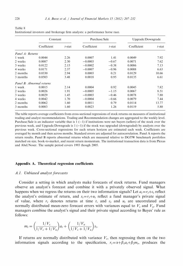
month and then across months. We compute t-statistics Fama-Macbeth style with acorrection for autocorrelation, as in Jegadeesh and Karceski (2009). We only includeobservations when both of the regressors are not zero. Similar to much of our earlieranalysis, we examine several alternative return horizons: those at one week, two weeks,three weeks, four weeks, two months, and three months.Table 8 reports the cross-sectional regression results. As before, Panel A reports the
results associated with raw returns while Panel B reports the results for DGTW-adjustedreturns. The upgrade/downgrade columns in Panel A indicate a strong relation betweenfuture returns and past analyst recommendation changes, as the recommendation changecoefficients are positive and statistically significant at all horizons. The results areconsistent with positive returns following upgrades and/or negative returns followingdowngrades. In contrast, the purchase/sale columns indicate that, after controlling forrecommendation changes, no relation exists between future returns and past institutionaltrades. In fact, the institutional trade variables are negative for all horizons but are notstatistically significant.The abnormal return results in Panel B of Table 8 mirror the raw return results in Panel
A. The coefficient on the upgrade/downgrade indicator variable is positive and stronglystatistically significant regardless of horizon, and the coefficient on the purchase/saleindicator is not significantly positive at any horizon. The size of the coefficients is alsoconsistent with the patterns evident in Tables 5 and 7, where the abnormal returns increasewith the horizon.Overall, the results in Table 8 indicate a strong correspondence between analyst
recommendation changes and future stock returns. When an analyst changes his recommenda-tion on a stock on the week that an institution buys or sells that stock, more often than not therecommendation change, rather than the institutional transaction, predicts the future return ofthe stock. After controlling for the recommendation change, no evidence exists of any relationbetween institutional trades and stock returns.
5. Conclusion
This paper evaluates the stock-selection skills of buy-side funds and sell-side analystsand examines their interactions. We find that stocks that funds buy significantlyoutperform stocks that they sell, but the difference in performance is largely concentratedon the day of the trade. Therefore, any superior information that funds may possess seemsto be fully revealed to the market through their trades. Consistent with earlier findings, wealso find that sell-side analysts’ recommendations are informative.Fund trades are related to past recommendation revisions, indicating that funds do use
analysts’ recommendations as factors in their trading decisions. In fact, fund trades are
20The model in the Appendix assumes the independent variables are continuous variables rather than binary
variables. Using continuous measures of recommendation changes and institutional trading (e.g., changes in
consensus recommendation or changes in fractional ownership of the firm) produces similar results.
Table 7
Performance of institutional investors’ trades following recommendation changes.
Purchases Sales Difference
Returns t-stat Returns t-stat Returns t-stat
Panel A: Performance of transactions following upgrades in the previous week
1 week 0.0096 4.58 0.0006 0.32 0.0090 4.51
2 weeks 0.0132 4.41 0.0049 1.69 0.0083 3.68
3 weeks 0.0159 3.80 0.0072 1.97 0.0087 2.52
4 weeks 0.0179 3.40 0.0101 2.16 0.0078 1.96
2 months 0.0366 3.48 0.0275 2.95 0.0091 1.61
3 months 0.0481 2.97 0.0400 2.97 0.0080 0.98
Panel B: Abnormal performance of transactions following upgrades in the previous week
1 week 0.0047 3.90 �0.0033 �2.29 0.0080 4.37
2 weeks 0.0054 2.92 �0.0020 �0.95 0.0073 2.92
3 weeks 0.0054 2.24 �0.0005 �0.20 0.0059 1.71
4 weeks 0.0049 1.90 0.0006 0.21 0.0042 1.13
2 months 0.0120 3.33 0.0047 1.22 0.0073 1.47
3 months 0.0111 2.46 0.0073 2.17 0.0039 0.81
Panel C: Performance of transactions following downgrades in the previous week
1 week 0.0061 3.73 �0.0027 �1.38 0.0087 6.30
2 weeks 0.0096 2.74 �0.0020 �0.68 0.0115 5.04
3 weeks 0.0103 2.03 0.0003 0.08 0.0100 3.05
4 weeks 0.0153 2.52 0.0026 0.49 0.0127 3.81
2 months 0.0259 2.17 0.0149 1.52 0.0110 1.72
3 months 0.0337 1.94 0.0257 1.89 0.0081 1.13
Panel D: Abnormal performance of transactions following downgrades in the previous week
1 week 0.0025 2.21 �0.0046 �3.64 0.0071 4.62
2 weeks 0.0040 2.21 �0.0054 �3.83 0.0094 4.57
3 weeks 0.0034 1.42 �0.0058 �2.76 0.0091 3.38
4 weeks 0.0062 2.25 �0.0055 �2.06 0.0117 4.06
2 months 0.0049 0.93 �0.0034 �0.79 0.0083 1.28
3 months 0.0066 1.01 �0.0015 �0.31 0.0081 1.27
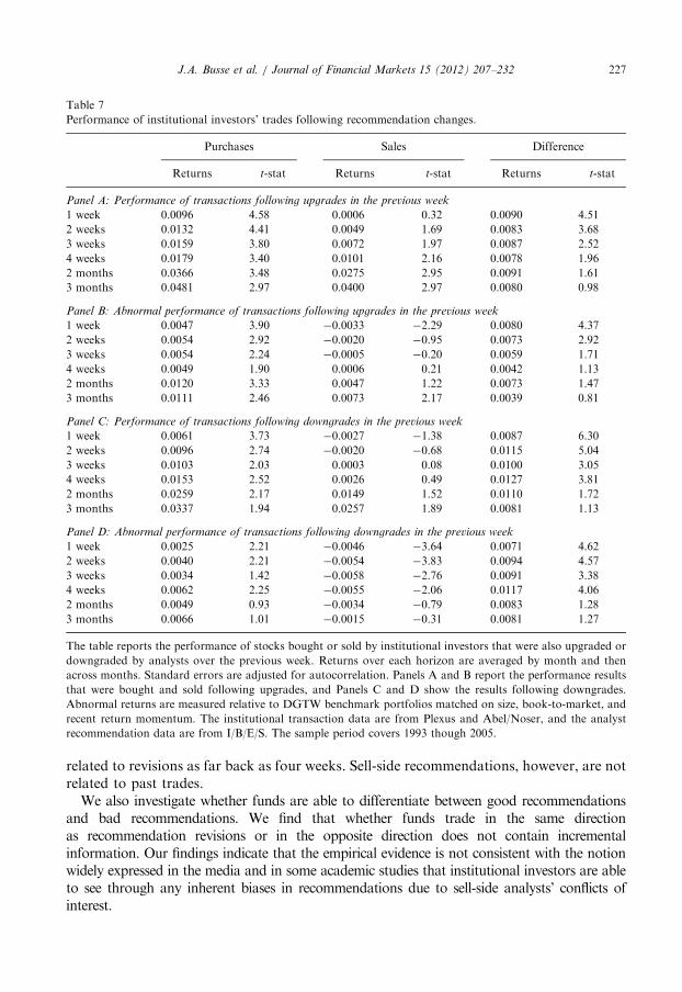
The table reports the performance of stocks bought or sold by institutional investors that were also upgraded or
downgraded by analysts over the previous week. Returns over each horizon are averaged by month and then
across months. Standard errors are adjusted for autocorrelation. Panels A and B report the performance results
that were bought and sold following upgrades, and Panels C and D show the results following downgrades.
Abnormal returns are measured relative to DGTW benchmark portfolios matched on size, book-to-market, and
recent return momentum. The institutional transaction data are from Plexus and Abel/Noser, and the analyst
recommendation data are from I/B/E/S. The sample period covers 1993 though 2005.
J.A. Busse et al. / Journal of Financial Markets 15 (2012) 207–232 227
related to revisions as far back as four weeks. Sell-side recommendations, however, are notrelated to past trades.
We also investigate whether funds are able to differentiate between good recommendationsand bad recommendations. We find that whether funds trade in the same directionas recommendation revisions or in the opposite direction does not contain incrementalinformation. Our findings indicate that the empirical evidence is not consistent with the notionwidely expressed in the media and in some academic studies that institutional investors are ableto see through any inherent biases in recommendations due to sell-side analysts’ conflicts ofinterest.
Table 8
Institutional investors and brokerage firm analysts: a performance horse race.
The table reports average coefficients from cross-sectional regressions of stock returns on measures of institutional
trading and analyst recommendations. Trading and Recommendation changes are aggregated to the weekly level.
Purchase/Sale is an indicator variable that is 1 (�1) if institutions were net buyers (sellers) of the stock over the
previous week, and Upgrade/Downgrade is 1 (�1) if the stock was upgraded (downgraded) by analysts over the
previous week. Cross-sectional regressions for each return horizon are estimated each week. Coefficients are
averaged by month and then across months. Standard errors are adjusted for autocorrelation. Panel A reports the
return results. Panel B reports abnormal returns which are measured relative to DGTW benchmark portfolios
matched on size, book-to-market, and recent return momentum. The institutional transaction data is from Plexus
and Abel/Noser. The sample period covers 1993 though 2005.
J.A. Busse et al. / Journal of Financial Markets 15 (2012) 207–232228
Appendix A. Theoretical regression coefficients
A.1. Unbiased analyst forecasts
Consider a setting in which analysts make forecasts of stock returns. Fund managersobserve an analyst’s forecast and combine it with a privately observed signal. Whathappens when we regress the returns on their two information signals? Let at¼rtþet reflectthe analyst’s estimate of return, and st¼rtþut reflect a fund manager’s private signalof value, where rt denotes returns at time t, and et and ut are uncorrelated andnormally distributed mean-zero forecast errors with variances equal to Ve and Vu. Fundmanagers combine the analyst’s signal and their private signal according to Bayes’ rule asfollows:
mt ¼1=Ve
1=Ve þ 1=Vu
� �at þ
1=Vu
1=Ve þ 1=Vu
� �st:
If returns are normally distributed with variance Vr, then regressing them on the twoinformation signals according to the specification, rt¼aþb1atþb2mt, produces the
J.A. Busse et al. / Journal of Financial Markets 15 (2012) 207–232 229
following regression coefficients:
b1 ¼ 0,
b2 ¼Vr
Vr þ1
ðð1=VeÞþð1=VuÞÞ
� � :
Thus, when fund managers observe analysts’ return forecasts, the managers’ signalincorporates the information and drives out the usefulness of the analysts’ signal in thereturn regression.
The coefficients can be derived as follows. From basic statistics, the coefficients will be:
b1 ¼Covr,aVarm�Cova,mCovr,m
VaraVarm�Cov2a,m
and
b2 ¼Covr,mVara�Cova,mCovr,a
VaraVarm�Cov2a,m
:
According to our assumptions, the variances and covariances are:
Vara ¼Vr þ Ve, Covðrþ e,rþ uÞ ¼Vr,Covðr,aÞ ¼Covðr,rþ eÞ ¼Vr,
Varm ¼Vr þ1=Ve
ð1=VeÞ þ ð1=VuÞ
� �2
Ve þ1=Vu
ð1=VeÞ þ ð1=VuÞ
� �2
Vu
¼Vr þ1
ð1=VeÞ þ ð1=VuÞ� � ,
Covðr,mÞ ¼Cov r,rþ1=Ve
ð1=VeÞ þ ð1=VuÞ
� �eþ
1=Vu
ð1=VeÞ þ ð1=VuÞ
� �u
� �¼Vr,
and
Covða,mÞ ¼Cov rþ e,rþ1=Ve
ð1=VeÞ þ ð1=VuÞ
� �eþ
1=Vu
ð1=VeÞ þ ð1=VuÞ
� �u
� �
¼Vr þ1
ð1=VeÞ þ ð1=VuÞ
� �,
which makes the coefficients simplify as follows:
b1 ¼Covr,aVarm�Cova,mCovr,m
VaraVarm�Cov2a,m
¼Vr Vr þ
1ðð1=VeÞ=ð1=VuÞ
� �� Vr þ
1ðð1=VeÞ=ð1=VuÞ
� �Vr
ðVr þ VeÞ Vr þ1
ðð1=VeÞ=ð1=VuÞ
� �� Vr þ
1ðð1=VeÞ=ð1=VuÞ
� �2 ¼ 0
J.A. Busse et al. / Journal of Financial Markets 15 (2012) 207–232230
and
b2 ¼Covr,mVara�Cova,mCovr,a
VaraVarm�Cov2a,m
¼VrðVr þ VeÞ� Vr þ
1ðð1=VeÞþð1=VuÞÞ
� �Vr
ðVr þ VeÞ Vr þ1
ðð1=VeÞþð1=VuÞÞ
� �� Vr þ
1ðð1=VeÞþð1=VuÞÞ
� �2 ¼ Vr
Vr þ1
ðð1=VeÞþð1=VuÞÞ
� � :
A.2. Biased analyst forecasts
We now consider a setting in which analysts purposefully add a bias to their signals ofvalue as a side effect of the other services they provide for their brokerage firms. Weassume that a fund manager’s skill involves deciphering recommendations to uncover theuseful investment advice. Let at¼rtþetþmt reflect analysts’ estimate of return with addedbias m�Nð0,VmÞ. Fund managers separate out the bias to create their private signal of valuemt¼at�mt, which is not observed by the overall market. In this setting, regressing returnson the two information signals according to the specification, rt¼aþb1atþb2mt, producesthe following regression coefficients:
b1 ¼ 0,
b2 ¼Vr
ðVr þ VeÞ:
Thus, when fund managers are able to observe analysts’ return forecasts and ‘‘seethrough’’ the bias, the fund manager’s signal incorporates the information and drives outthe usefulness of analysts’ signals in the return regression.The coefficients are derived as follows. From basic statistics the coefficients will be;
b1 ¼Covr,aVarm�Cova,mCovr,m
VaraVarm�Cov2a,m
and b2 ¼Covr,mVara�Cova,mCovr,a
VaraVarm�Cov2a,m
:
Under our assumptions, the variances and covariances are: