1 DIFFUSION OF LIGHT GASES IN NANOSTRUCTURED SORBENTS By AAKANKSHA KATIHAR A THESIS PRESENTED TO THE GRADUATE SCHOOL OF THE UNIVERSITY OF FLORIDA IN PARTIAL FULFILLMENT OF THE REQUIREMENTS FOR THE DEGREE OF MASTER OF SCIENCE UNIVERSITY OF FLORIDA 2011
Transcript
1
DIFFUSION OF LIGHT GASES IN NANOSTRUCTURED SORBENTS
By
AAKANKSHA KATIHAR
A THESIS PRESENTED TO THE GRADUATE SCHOOL OF THE UNIVERSITY OF FLORIDA IN PARTIAL FULFILLMENT
OF THE REQUIREMENTS FOR THE DEGREE OF MASTER OF SCIENCE
Molecular Transport and Diffusion .......................................................................... 14
Experimental Study of Diffusion at Micrometer Length Scale ................................. 17 Diffusion Measurements using Pulsed Field Gradient Nuclear Magnetic
Basics of NMR .................................................................................................. 18 Longitudinal and transverse magnetization ................................................ 19
Relaxation: spin-lattice and transverse ...................................................... 21 Signal detection ......................................................................................... 23
2-1 Self-diffusivities of the cation, anion and CO2 by 13C PFG NMR in the sample of [bmim][Tf2N] with different 13CO2 loadings and at different temperatures ...... 37
2-2 Activation energy of self-diffusion for the cation, anion, and CO2 for different CO2 loadings ...................................................................................................... 41
8
LIST OF FIGURES
Figure page
1-1 Schematic representation of spin precession in presence of an external magnetic field ..................................................................................................... 19
1-2 Schematic representation of longitudinal net magnetization in presence of external magnetic field ........................................................................................ 20
1-3 Schematic of Pulsed Field Gradient Nuclear Magnetic Resonance (PFG NMR) stimulated echo pulse sequence .............................................................. 25
1-4 Schematic of the PFG NMR stimulated echo longitudinal encode decode pulse sequence .................................................................................................. 26
1-5 Schematic of the PFG NMR stimulated echo pulse sequence with bipolar gradients ............................................................................................................. 28
2-1 Comparison between the attenuation curves obtained from proton and carbon-13 (C-13) PFG NMR experiments .......................................................... 36
2-2 Proton and C-13 NMR spectra of [bmim][Tf2N] with a 13CO2 loading of 0.011 carbon dioxide molecules per anion-cation pair.................................................. 38
2-3 C-13 PFG NMR attenuation curve measured for the sample of [bmim][Tf2N] with a 13CO2 loading of 0.15 13CO2 molecules per anion cation pair ................... 40
2-4 The dependence of the self-diffusion coefficient for the cation, anion and 13CO2 on the concentration of 13CO2 inside the ionic liquid ................................ 41
2-5 Temperature dependence of the self-diffusivity for the sample of [bmim][Tf2N] with the 13CO2 loading of 0.063 CO2 molecules per cation-anion pair ..................................................................................................................... 42
3-1 Scanning Electron Microscope (SEM) images of aluminosilicate single walled nanotubes (SWNTs) bundles.............................................................................. 45
3-2 Attenuation curves for diffusion measurements of tetrafluoromethane in aluminosilicate nanotubes obtained for different effective diffusion times .......... 49
3-3 PFG NMR attenuation curves for tetrafluoromethane in aluminosilicate nanotubes at effective diffusion time of 4 ms extended to larger gradients ........ 50
9
LIST OF ABBREVIATIONS
FID Free Induction Decay
IL Ionic Liquid
MSD Mean square displacement
NMR Nuclear Magnetic Resonance
PFG NMR Pulsed Field Gradient Nuclear Magnetic Resonance
A g Amplitude of PFG NMR signal as a function of magnetic field
gradient g
0B The amplitude of the applied external static magnetic field
1B The amplitude of the oscillating applied magnetic field due to a
radio frequency pulse
effB The amplitude of net effective magnetic field
c Concentration of molecules or ions
C A constant in the Stokes-Einstein equation
D Diffusion coefficient
E Activation energy for diffusion
g Amplitude of the magnetic field gradient
J Flux of molecules or ions
10
k Boltzmann constant
X YM Amplitude of net transverse magnetization
zM Amplitude of net magnetization along z axis
0M Equilibrium value of net magnetization along z axis
P Probability density
2r Mean square displacement
R Gas constant
S Spin angular momentum
t Time
1t Duration between the first and the second r.f. pulse in 2D NMR
exchange spectroscopy pulse sequence
2t The duration of signal acquisition in 2D NMR exchange
spectroscopy pulse sequence
efft Effective diffusion time
T Absolute temperature
1T Longitudinal (Spin-Lattice) NMR relaxation time
2T Transverse (Spin-Spin) NMR relaxation time
LEDT Duration between the fourth and fifth r.f. pulse in PGSTE-LED pulse
sequence for eddy current dissipation
v t Velocity as a function of time
z z coordinate of position of molecule/ion/ nuclear spin
Gyromagnetic ratio
Duration of magnetic field gradient pulse
Diffusion time
11
Magnetic moment of a nuclear spin
Duration between 2
and r.f. pulse in PFG NMR spin echo
pulse sequence
1 Duration between the first and second r.f. pulse in PFG NMR
stimulated echo pulse sequence
2 Duration between the second and third r.f. pulse in PFG NMR
stimulated echo pulse sequence
p Duration of the r.f. pulse
i The phase angle of individual spin magnetization vectors
Flip angle of a r.f. pulse
Amplitude of signal attenuation in PFG NMR experiment
Larmor frequency
ref Larmor frequency of reference nuclei
SF01 Operating frequency of NMR spectrometer
12
Abstract of Thesis Presented to the Graduate School of the University of Florida in Partial Fulfillment of the Requirements for the Degree of Master of Science
DIFFUSION OF LIGHT GASES IN NANOSTRUCTURED SORBENTS
By
Aakanksha Katihar
December 2011 Chair: Sergey Vasenkov Major: Chemical Engineering
In this work the potential of pulsed field gradient nuclear magnetic resonance
(PFG NMR) at high magnetic field and high magnetic field gradients for uncovering the
relationship between the structural and transport properties of nanostructured sorbents
is explored and demonstrated. The systems under study can be divided into two types:
(i) organized soft matter systems (room temperature ionic liquids): and, (ii) porous solids
(aluminosilicate nanotubes).
In the first part of the work, the reported diffusion studies are focused on room
temperature ionic liquids and their mixtures with carbon dioxide. The effect of absorption
of CO2 in RTILs on diffusion properties is investigated and discussed. The results also
help to estimate the diffusion coefficients of all the three species i.e., the cation, anion
and CO2.
In the later part of the work, diffusion of a light gas tetrafluoromethane in a new
type of inorganic nanotubes (aluminosilicate nanotubes) is discussed. The measured
data show that there are two ensembles of gas molecules. The first ensemble consists
of molecules undergoing intra-channel diffusion, while the other represents molecules
undergoing long-range diffusion. The results allow the estimation of the diffusivity of
13
tetrafluoromethane inside the nanotubes as well as the diffusivity for these molecules
undergoing fast exchange between many nanotubes. The results were found to support
the assumption about the one-dimensional nature of the tetrafluoromethane diffusion
inside nanotubes.
14
CHAPTER 1 INTRODUCTION
Molecular Transport and Diffusion
Since a long time, diffusion has been defined as tendency of matter (molecules,
ions etc.), at temperatures above absolute zero, to migrate randomly in such a way as
to eliminate spatial variations in concentration or densities. However it is now known
that the real driving force for diffusion is a gradient of chemical potential. Diffusion can
be differentiated in two different processes: Transport diffusion (which involves
movement of molecules in order to reduce gradients of chemical potential) and Self
diffusion (random motion of matter that takes place even when there is no chemical
potential or concentration gradients and is driven by thermal energy).
The study of diffusion dates back to 1850s when Adolf Fick started his
experimental studies and came up with Fick‟s first law of Diffusion1,2 for one dimensional
diffusion
(1.1)
where is the flux of the diffusing molecules/ions along the direction, is their
concentration and is the corresponding diffusion coefficient known as transport
diffusion coefficient. It relates flux of molecules and concentration/chemical potential
gradient under non equilibrium conditions.
If, however, a fraction of molecules in a sample is tagged or labeled, similar
equation can be developed for self-diffusion as well. Here an assumption needs to be
made that there is an uneven distribution of the labeled and unlabeled molecules while
overall molecular concentration remains the same at any point in the system. Thus self-
diffusivity or self-diffusion coefficient (for one-dimensional diffusion) can be defined as
15
(1.2)
where is concentration of labeled molecules while the total concentration remains
constant and is the flux of the labeled molecules. For three-dimensional diffusion
(transport or self), Equation 1.2 becomes
(1.3)
where will be the diffusion coefficient (can be transport or self) in direction due to
concentration gradient in direction. Equation 1.1 along with the principle of
conservation of mass leads to Fick‟s second law for one dimension, which is written as
(1.4)
When is independent of concentration Equation 1.4 takes the following form
(1.5)
Again for the case of three-dimensional diffusion with concentration-independent
diffusivity (self or transport), Fick‟s second law can be written as
(1.6)
For the case of closed system (where the total mass of diffusing species remains
constant) and isotropic diffusion (where the self-diffusion coefficient is equal in all
directions) the concentration distribution is given by3
(1.7)
16
where is the total mass of the diffusing species and is a probability function or
Diffusion Propagator4 and gives probability of finding a molecule/ion at a certain position
at time . This is a Gaussian function, variance of which gives the mean square
displacement
(1.8)
Using Equation 1.8, we get the following expressions for mean square displacements of
molecules/ions for 1, 2 and 3 dimensional isotropic diffusion
(1.9)
(1.10)
(1.11)
Equations 1.9 to 1.11 are called Einstein Relations.4
Studying molecular transport on small length scales is important as it not only
helps to understand various system properties but also controls them on macroscopic
length scales. The primary mechanism of molecular transport is related to self-diffusion
and thus investigation of self diffusion under the conditions of interest becomes
indispensible in order to study molecular transport at small length scales. This work
reports self-diffusion of light gases in complex nanostructured materials, which are
heterogeneous on length scales from nanometer to several micrometers. Due to their
heterogeneity on such length scales, these materials exhibit a lot of unique and
interesting properties important for industrial applications. The systems selected for this
work are of two types: 1) organized soft matter systems (room temperature ionic liquids)
and 2) porous solids (aluminosilicate nanotubes).
17
Experimental Study of Diffusion at Micrometer Length Scale
To study diffusion on different length scales, different techniques can be used. The
main experimental technique used in this work is high field (17.6 T) and high gradient
(up to 30 T/m) pulsed field gradient nuclear magnetic resonance (PFG NMR).
PFG NMR technique has proven to be a powerful tool for the study of diffusive5,6,7
molecular motions. High field and high gradient PFG NMR is a non-invasive technique
that combines the advantages of high-field and high magnetic field gradients for
diffusion studies. High magnetic field helps to achieve high sensitivity, while application
of high gradients allows for diffusion studies on small length scales using nuclei with
small gyromagnetic ratios (such as C-13). The next section discusses the theory of PFG
NMR in detail.
Diffusion Measurements using Pulsed Field Gradient Nuclear Magnetic Resonance (PFG NMR)
All substances have the capability of interacting with magnets. The microscopic
sources of this magnetism are: 1) circulation of electric currents (due to the electrons),
2) the magnetic moments of the electrons and 3) the magnetic moments of the nuclei.
Nuclear magnetic resonance (NMR) spectroscopy uses the nuclear magnetism (due to
their magnetic moment or spin) associated with some nuclei. This intrinsic nuclear
magnetism can be exploited in the presence of an external magnetic field (B0) by
applying electromagnetic radio frequency (r.f.) pulses. When these r.f pulses are applied
under the conditions of resonance, the nuclei absorb energy which is radiated back and
is received as the signal by a coil. The signal contains a lot of information about the
structure and dynamics of the molecules containing the nuclei.
18
Basics of NMR
Spin angular momentum or just spin is an intrinsic quantum-mechanical property
of atomic nuclei. This is related to the magnetic moment as shown below
(1.12)
where is the magnetic moment and S is the spin angular momentum. The direction of
the spin angular momentum is also called the spin polarization axis. Equation 1.12
suggests that nuclei which have a non-zero value of spin exhibit magnetism as they
have a non- zero magnetic moment. , which is called the gyromagnetic or
magnetogyric ratio, is a property of the nuclei and can be positive or negative. The sign
determines whether magnetic moment will be aligned in the direction or opposite to the
direction of the spin or the direction of spin polarization.
When there is no external field, these magnetic moments are randomly aligned
and there is no net nuclear magnetization. As soon as a magnetic field is switched on, it
exerts a torque on the magnetic moment which in turn forces the spin polarization to
start moving around the field on a cone at a constant angle (the constant angle depends
on angle between initial spin polarization vector and the field) between direction of spin
polarization and the field (Figure 1-1). This is called precession and is a result of
intrinsic spin angular momentum of the nuclei. The external magnetic field B0
determines the frequency of precession (also called the Larmor frequency8,9) as
given by the Equation 1.13
(1.13)
19
+z
(b)B0
(a)B0
+z
Figure 1-1. (a): Schematic representation of spin precession in presence of an external magnetic field B0 (b): The angle of the precession cone depends on initial spin polarization.
Longitudinal and transverse magnetization
In the absence of an external magnetic field, the distribution of the spin
polarizations is isotropic and thus there is no net magnetization in the sample (Figure 1-
2a). As soon as an external field is switched on all the spins start executing precession
around the field. But the distribution of spin polarizations still remains isotropic and
consequently the total magnetic moment of the material does not change. However,
microscopically, each nuclear spin is surrounded by other magnetic entities, (i.e., other
nuclear spins and electron clouds) and switching on the field leads to formation of local,
microscopic magnetic fields around each nucleus which fluctuate rapidly in both
magnitude and direction because of the thermal agitation of the environment. These
microscopic fluctuating fields result in a gradual breakdown of constant angle spin
precession of the nuclear spins and the magnetic moments of the nuclear spins wander
between different precession angles eventually sampling all possible orientations. This
process brings about anisotropy in distribution of spin polarization directions and the
resulting steady-state distribution of spin polarizations is slightly biased towards an
20
orientation with lower energy where spin orientations have corresponding magnetic
moments along the direction of the applied magnetic field (Figure 1-2b). This is referred
to as longitudinal magnetization as the direction of the external magnetic field and
resulting nuclear magnetization is assumed to be in the +z direction (or longitudinal
direction) of the static coordinate system.
B0
Smi = M0(a) (b)Smi = 0
Net magnetic
moment
Figure 1-2. (a) No magnetization in absence of external magnetic field. (b) Schematic representation of longitudinal net magnetization when external magnetic field
B0 is switched on. The longitudinal magnetization 0M is the vector sum of
individual magnetic moments im 8.
Nuclear magnetization is very small as compared to magnetization produced by
other mechanisms (electronic magnetization, bulk magnetization etc). Thus, detection of
longitudinal magnetization becomes extremely difficult. Thus in NMR, magnetization in a
transverse plane is detected. This is done by applying an orthogonal oscillating
magnetic field (which has a frequency close to Larmor frequency and magnitude
smaller than ) by passing an alternating current through a coil. Application of the
field is called application of r.f. pulses as the Larmor frequencies are typically in the
range of radio waves. Once the magnetization is tilted in the transverse (X-Y) plane, it
21
starts precessing and when the r.f. pulse is turned off it gradually returns to the
equilibrium direction of the static external magnetic field 0B . This process of relaxation is
discussed in the next section.
Thus the basic idea of NMR is to apply a torque that is orthogonal to the torque
exerted by the static magnetic field on the spins and that varies with time in exact
frequency match with the natural precession frequency of the nuclear spins. This is
achieved by applying a magnetic field that is orthogonal to the main magnetic field and
oscillating in time in exact synchrony with the precession frequency of the atomic nuclei.
Relaxation: spin-lattice and transverse
In the presence of static magnetic field the net magnetization is in the
longitudinal direction. This is the equilibrium condition and when an r.f. pulse is applied,
it tilts the magnetization in transverse plane and results in a non-equilibrium condition.
As time passes, the net magnetization returns back to its equilibrium state -- a process
known as NMR relaxation. This is of two types: 1) Spin-Spin/Transverse, or 2T
relaxation (which is the gradual decay of transverse magnetization to zero) and 2) Spin-
Lattice/Longitudinal, or 1T relaxation (which is the gradual growth of net nuclear
magnetization to its equilibrium value in the +z direction)8-10.
Just after the r.f. pulse is applied and net magnetization is turned to transverse
plane, all the spins remain in phase coherence. It is due to disturbances in local
magnetic field by neighboring magnetic entities (like other nuclear spins and electronic
clouds) that as time progresses, various spins in the sample de-phase (called the
secular contribution to T2 relaxation). As a result, the net transverse magnetization
gradually decays to zero.
22
Another reason of transverse relaxation is the presence of fluctuating, microscopic
magnetic fields. These fields might exhibit frequencies in the range of Larmor
frequency, thereby acting as tiny r.f. pulses, gradually turning the magnetic moments
away from the X-Y plane (called the non-secular contribution to T2 relaxation). The net
rate of transverse relaxation can be characterized by a time constant 2T , as shown in
Equation 1.14
(1.14)
where x yM t is the net transverse magnetization at time and 2T is the spin-
spin/transverse NMR relaxation time constant.
Immediately after the application of r.f. pulse, the longitudinal magnetization is
zero. Disturbances that cause the non-secular part of 2T NMR relaxation can also cause
the 1T NMR relaxation process. In addition, the nuclear spins experience perturbations
in the local magnetic field due to rapid molecular tumbling. These local fields try to
reorient individual nuclear spin magnets and orientations with the magnetic moment
along the direction of the field are favored as they have lower energy. This is also
responsible for re-growth of the magnetization along the z axis to the equilibrium value,
the rate of which can be characterized by the longitudinal relaxation time 1T
(1.15)
where zM t is the net longitudinal magnetization at time t , 0M is the net equilibrium
magnetization, which points along +z direction and is longitudinal relaxation time
constant.
23
Signal detection
The signal is detected by a coil placed near the sample. The continuously
changing magnetic field (changing because of the precession of spins in the transverse
plane) induces an electric current in the coil according to the Maxwell‟s law. This is
detected as a signal gradually decaying with time and is referred to as free Induction
decay (FID).Fourier transformation of the FID gives frequency domain data known as
NMR spectra.
Again due to variations in the local magnetic field experienced by individual spins
the resonance frequencies of all nuclei show small deviations from the Larmor
frequency. This effect is known as chemical shift. Thus the resonance frequencies and
in turn the chemical shifts of same element in different chemical environments are
different i.e., 1H in a CH3 group will have a different chemical shift than that of 1H in CH2
or 1H in water. Thus knowing the chemical shift data allows identifying different atomic
environments and helps in investigating the properties of the system under
consideration.
Resonance frequencies are magnetic field dependent and thus they can vary from
one experimental setup to another. To overcome this problem and to simplify
comparison of data measured at different amplitudes chemical shifts are calculated in
parts per million (ppm) units instead of frequency units using the Equation 1.16.
(1.16)
where is the chemical shift in ppm, the measured frequency, ref is the reference
frequency and SF01 is the so called „Carrier Frequency‟ i.e. the operating frequency of
the magnet.
24
Thus some ideas worth noting about NMR are: 1) the strength of the magnetic
field determines the amount of magnetization in the atomic nuclei at thermal equilibrium
and the precession frequency of the nuclei. 2) The coil is used to produce an oscillating
magnetic field that is in resonance with nuclei and causes the torque that tips the
magnetization out of equilibrium in the transverse plane. 3) The same coil is not only
used to transmit to the nuclei but also used to receive the signal i.e, to pick up the
Electro Motive Force (EMF) at oscillating voltage as the nuclear magnetization
precesses around the coil with signal gradually decaying with time as the spins come
back to their equilibrium value.
Pulsed Field Gradient (PFG) NMR
PFG NMR makes use of the fact that the Larmor frequency of the precession of
the nuclear spins is field dependent. In PFG NMR, when magnetization is in the
transverse plane, a gradient of magnetic field is applied along the z direction.
Application of magnetic field gradients makes the Larmor frequency position dependent
(according to Equation 1.18) and thus helps in labeling the nuclear spins based on their
spatial coordinate along the z-direction
(1.17)
where is the Larmor frequency, is the gyromagnetic ratio, 0B denotes static external
magnetic field; g is the linear gradient of the magnetic field superimposed on the 0B
field and z is the coordinate along the z axis. The pulse sequences used in this work
are explained in detail in the next few sections.
25
PFG NMR stimulated echo pulse sequence
/2 /2 /2
1 2 1
gradient gradientg g
FID
Figure 1-3. Schematic of PFG NMR stimulated echo pulse sequence. This sequence is
of great advantage for systems in which the 2T NMR relaxation time is much
shorter than 1T NMR relaxation time.
Figure 1-3 shows the schematic of the standard PFG NMR stimulated echo pulse
sequence which consists of three 2
pulses and two field gradients of identical
amplitude g and duration . The first r.f. pulse brings the longitudinal magnetization to
the transverse plane and the first field gradient pulse labels the spins according to their
spatial coordinate in the z direction. In the process of such labeling the spins precess
with different Larmor frequencies given by Equation 1.18 and consequently dephase.
Hence the time interval between the two pulses is called the de-phasing interval. The
time interval is approximately equal to the effective diffusion time used to measure
diffusivity. Following the dephasing the net magnetization is tilted to –z direction by the
second 2
r.f. pulse and again to the transverse plane by the third one. Again a field
gradient of the same duration and amplitude is applied. During this (second) gradient
pulse the individual spin magnetization vectors experience rephrasing. Hence the time
26
interval between the third r.f. pulse and the beginning of acquisition is called the
rephasing interval. If molecules diffuse during the time between gradient pulses, the
refocusing of the magnetization is not complete and final intensity is lesser than the
maximum intensity. This decrease in amplitude of the intensity contains information
about diffusion of the molecules.
This pulse sequence is particularly advantageous for diffusion studies of systems
which experience slower decay of magnetization due to longitudinal 1T relaxation (i.e,
relaxation during the time interval of duration ) than that due to transverse 2T (i.e,
relaxation during the two time intervals of duration 1 ).Another advantage of using this
pulse sequence is that the diffusion time can be increased in this pulse sequence by
Figure 1-4. Schematic of the PFG NMR stimulated echo longitudinal encode decode pulse sequence.
In a PFG NMR experiment, the gradient pulses are repeatedly switched on and
off. This generates eddy currents in the coil and in turn inhomogeneities in the magnetic
field. These undesirable inhomogeneities can be avoided by using PFG NMR stimulated
27
echo longitudinal encode-decode or longitudinal eddy current delay pulse sequence
(PGSTE-LED)11 which is a modified form of the PFG NMR stimulated echo pulse
sequence (Figure 1-4). The difference being that there are two additional r.f. pulses
separated by the time LEDT at the end of this sequence. Using these r.f. pulses, the
direction of the net magnetization is changed to longitudinal plane (-z direction) from the
transverse plane for the time LEDT and then brought back to the transverse plane. This
time delay between the end of second field gradient pulse and the beginning of
acquisition helps to dissipate the eddy currents.
In the stimulated pulse sequence, to introduce a delay between the end of the
second gradient pulse and the beginning of acquisition, same delay has to be
introduced between the end of the first gradient pulse and the next r.f. pulse thereby
increasing the time for which the net magnetization is in the transverse plane and
reducing the signal by T2 relaxation. This problem is not encountered in PGSTE-LED
sequence as the net magnetization is taken from the transverse plane to the longitudinal
direction (-z) axis, which is followed by the LED delay LEDT . During the LED delay, signal
is reduced only due to 1T NMR relaxation. This is an advantage over the other
sequences for the measurement conditions which are likely to introduce disturbing eddy
currents.
PFG NMR stimulated echo with bipolar gradients pulse sequence
The pulse sequences discussed above use unipolar gradients. Figure 1-5 shows a
schematic for the PFG NMR stimulated echo pulse sequence with bi-polar gradients12-
15, also called the 13-interval sequence.
2
28
FID
1 2 1
gradient
gradient gradient
gradient
1 1
g
g
g
g
/2 /2 /2 /2
Figure 1-5. Schematic of the PFG NMR stimulated echo pulse sequence with bipolar gradients. Bipolar gradients are used to suppress internal gradients.
In a heterogeneous media, the magnetic susceptibility variations cause some
background magnetic field gradients. This may lead to signal attenuation and may even
introduce artifacts in the measurements of self-diffusion. These problems are reduced
by using PFG NMR stimulated echo pulse sequence with bipolar gradients (Figure 1-5).
Each of the two positive field gradient pulses of duration 2 and amplitude g in the
PFG NMR stimulated echo pulse sequence is replaced by a pair of gradient pulses,
each of duration and amplitude g , with opposite polarity separated by a r.f.
pulse. This sequence eliminates influence of the background gradients (those that have
the same polarity and amplitude over the duration of the sequence) on the measured
signal.
Generalized Attenuation Equation
The signal attenuation can be related to the molecular diffusion by determining the
net phase accumulated by the spins (Equation 1.19) and calculating the vector sum of
individual magnetic moments by the end of the pulse sequence.
29
(1.18)
where 0effB B= for the cases where there is no field gradient and
0effB B gz= in the
presence of field gradient pulses. The duration of field gradient is taken to be much
smaller than diffusion interval. Thus for a spin diffusing from position to the net
phase accumulated will be given as
(1.19)
The net transverse magnetization at any time will be proportional to cosine of the net
phase as projection of magnetization vectors in the direction of transverse
magnetization (immediately after first r.f. pulse is applied) is proportional to it. Using this
and the conditional probability 1 1p z dz (probability of finding a molecule at any position
between and ) with the corresponding one dimensional diffusion propagator
2 1 2, ,P z z dz , the net transverse magnetization at the end of the spin echo pulse
sequence10,16 can be written as
(1.20)
Now, the signal attenuation is given by the ratio of attenuated signal (in presence of
field gradients) to the signal recorded in the absence of any field gradients i.e.
(1.21)
where is the signal intensity at the gradient g and is the signal intensity at
zero gradient. Equation 1.21 can be written in terms of signal attenuation as
1z 1 1z dz
30
(1.22)
For a homogenous medium and for normal (i.e., Fickian diffusion) 1 1p z = 17 and
2 1, ,P z z is given by Equation 1.23
(1.23)
By combining these equations signal attenuation can be simplified to the Equation 1.24
(1.24)
where is the gradient duration, efft denotes the effective diffusion time and denotes
the self diffusion coefficient or self diffusivity.
The general form of attenuation equation for normal isotropic diffusion used for all
the pulse sequences discussed above can be simplified to the following form
(1.25)
where k g = for PGSTE/ PGSTE-LED pulse sequences and 2k g = for the 13-
interval pulse sequence. The effective diffusion time efft for both PGSTE and PGSTE-
LED is given by Equation 1.26 and for the 13-interval sequence, it is given by Equation
1.27
(1.26)
(1.27)
Substituting Einstein relation into Equation 1.26 gives Equation 1.28 for isotropic one
dimensional diffusion in the direction of field gradients and Equation 1.29 for isotropic
three-dimensional diffusion
31
(1.28)
(1.29)
where
2
2
zis the mean square displacement in the direction of the field gradients and
2 2 2 2 23r x y z z= = . In PFG NMR experiments, signal attenuation is
determined as a function of square of the amplitude i.e., keeping all other parameters
of the pulse sequence constant. These are the so-called PFG NMR attenuation curves
that are used to determine mean square displacements and the corresponding
diffusivities using above mentioned equations.
As attenuation is the ratio of signal at a particular gradient to the signal at zero
gradient, contribution of NMR relaxation remains the same for both and thus does not
make any contribution to the PFG NMR attenuation.
32
CHAPTER 2 ROOM TEMPERATURE IONIC LIQUIDS
Room temperature ionic liquids (or RTILs) are molten salts that are liquid around
room temperature. Generally, they are composed of a large asymmetric organic cation
and either an organic or inorganic anion18. It is believed that the low melting point of
ionic liquids is a result of the asymmetry of the cation and the nature of the anion is
considered to be responsible for a lot of their interesting physical properties such as
miscibility with conventional solvents, hygroscopicity, etc19. The most commonly studied
RTILs are imidazolium based salts which are not only easy to synthesize but also have
interesting physical properties that make them highly useful for many chemical
processes. A good thing about ionic liquids is that their physical properties can be made
“task specific” by judiciously selecting cation, anion, and their substituents20. Some of
these tailor-made or “task-specific” ionic liquids have proven very useful in both
synthetic and separations applications21-23.
Motivation
Ionic liquids are getting a lot of scientific attention because of their unique and
interesting properties. These liquids have high solubility for polar as well as non-polar
compounds and they can simultaneously dissolve organic and inorganic substances,
they have negligible vapor pressure, a stable liquid range of up to 400 K, excellent ionic
conductivity, thermal stability and their density is greater than water. Due to these
properties, RTILs are used as media for gas and liquid separations24-26, solvents for
homogeneous catalysis for a variety of organic reactions24,27-29, electrolytes for batteries
and fuel cells30,31, heat transfer/storage fluids and lubricants20,24,32,33 and are also being
33
considered as “green solvents” for various separation processes because they are
nonvolatile, nonflammable, and thermally stable34.
By far one of the most attractive approaches for the separation of a compound
from a mixture of gases is absorption into a liquid. Ionic liquids, because of their
properties like negligible vapor pressure and thermal stability, have been proposed as
solvent reagents for gas separations35. However, fundamental understanding of
transport properties of mixtures of RTILs with carbon dioxide is essential for potential
applications of RTILs for CO2 separations. Such applications are feasible in view of the
recent results indicating that the absorption capabilities of RTILs for CO2 can be quite
high36-40.
Diffusion studies of CO2 in RTILs have been reported in the literature but these
studies, until now, were performed by “macroscopic” techniques, which are based on
measurements of gas fluxes through macroscopic IL samples41-43. This work focuses on
studies of the influence of absorption of carbon dioxide into an imidazolium based RTIL
on the diffusion properties of ions. In addition, the diffusion of CO2 in mixtures of the
ionic liquid with carbon dioxide was also studied. Both 13C and proton pulsed field
gradient nuclear magnetic resonance (PFG NMR) were used to study self-diffusion in
the mixtures.
PFG NMR Experiment Details
Sample Preparations
The RTIL chosen for the study was 1-Butyl-3-methylimidazolium
bis(trifluoromethylsulfonyl)imide ([bmim][Tf2N]) and was purchased from Ionic Liquid
Technologies (99% purity). The samples of RTIL mixtures with carbon-13 labeled CO2
were prepared by the following procedure. Five 5 mm NMR tubes were filled with the
34
chosen RTIL. In all cases the sample height in a vertically-oriented tube was kept
around 12 mm or smaller to make sure that there are no effects of convection on the
data measured at elevated temperatures. These samples were then evacuated under
high vacuum at around 100 degree Celsius for 24 hours to remove any moisture
present. The loading of CO2 was then performed either by exposing the dry liquid to
CO2 gas at a fixed pressure for at least 4 hours or by cryogenically transferring the
required amount of CO2 from the calibrated volume of the vacuum system into the NMR
tube using liquid nitrogen. After this, the tubes were flame-sealed.
The 13CO2 loading or the amount of carbon-dioxide in the mixtures of RTIL and
CO2 is expressed as number of carbon dioxide molecules per anion-cation pair. This
13CO2 loading inside the IL was calculated using the following data: (i) Henry‟s law
constants reported in43 for carbon dioxide absorption into [bmim][Tf2N], (ii) known mass
of CO2 introduced into the tubes with the IL before they were sealed, and (iii) known
volumes of the IL and the gas phase in the sealed NMR tubes. One of the tubes
contained pure IL with no carbon dioxide while the others had increasing carbon-dioxide
loadings of 0.033, 0.063, 0.15 and 0.35 carbon dioxide molecules per anion-cation pair.
Pulsed Field Gradient (PFG) NMR Studies
1H and 13C PFG NMR diffusion studies were carried out using a wide bore 17.6 T
Bruker Biospin spectrometer. Magnetic field gradients were generated using diff60
diffusion probe (Bruker Biospin) and Great60 gradient amplifier (Bruker Biospin). The
diffusion experiments were done over a broad range of temperatures from 297 to 351 K.
and were repeated under the same conditions to make sure the reproducibility of data.
In most cases, diffusion studies were performed by using the standard PFG NMR
stimulated echo pulse sequence. The absence of susceptibility effects and
35
measurement artifacts was confirmed: (i) by verifying that the diffusion data obtained
under same conditions but at different magnetic field amplitudes were the same within
the limits of experimental uncertainty, and (ii) by the fact that 1H and 13C PFG NMR
diffusion data measured for the same diffusing species in the same samples and under
the same conditions were found to coincide within the limits of experimental error
(Figure 2-1). Also in each case the self diffusivity was calculated for two diffusion times
(8.6 ms and 38.6 ms) to ensure that the convection effects do not affect the data under
the measurement conditions.
The signal intensity was determined by integrating the area under selected line(s)
of the spectra recorded by the PFG NMR pulse sequence or by using the amplitudes of
these line(s). Figure 2-2 shows an example of the proton and 13C NMR spectra for a
mixture of [bmim][Tf2N] and carbon dioxide. Different lines in such spectra can
correspond to different species. Hence, for data processing, it becomes essential to
select appropriate line (or lines) for each type of species. For the lines in the NMR
spectra that originate from the diffusing species in the same types of local environments
and that exhibit no significant overlap with the lines of other types of ions/molecules in a
sample, Equation 1.25 was used to determine the diffusivity. However when the
selected line has contributions either from species in different types of domains or from
different types of molecules and/or ions having different diffusivities, the attenuation
curves are described as a sum of two or three weighted exponential terms of the type
shown in Equation 2.1
(2.1)
36
where and respectively represent the fraction and diffusivity of ensemble .
Figure 2-1. Comparison between the attenuation curves obtained from 1H (●) and 13C (▲) nuclear magnetic resonance (NMR) experiments. The 1H NMR experiment was done using a 13-interval pulse sequence and the 13C NMR experiments were done using a stimulated echo pulse sequence.
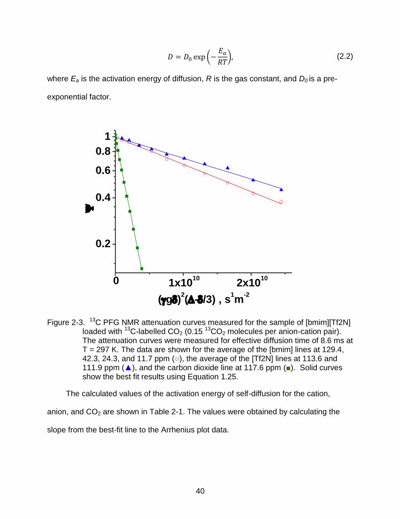
Results and Discussion
Table 2-1 shows the self-diffusion coefficients for each species at all temperatures
and CO2 loadings. Figure 2-3 shows an example of the results of self-diffusion
measurements for a mixture of ([bmim][Tf2N]) and 13CO2 (A loading of 0.15 CO2 per
anion-cation pair). All attenuation curves in Figure 2-3 are monoexponential in
agreement with Equation 1.25. As expected of all the three species, CO2 has the fastest
diffusivity (the slope of the attenuation curve is the largest). However the cation diffuses
faster than the anion in spite of being larger in size than the anion. Such behaviour is
attributed to the existence of well-defined local structures in the pure
0.0 4.0x10¹⁰
8.0x10¹⁰
0.1
1
13C: (g
2(-/3), s
1m
-2
1H: (g
2(-/2-/6), s
1m
-2
37
Table 2-1. Self-diffusivities of [bmim]+, [Tf2N]- and CO2 recorded by 13C PFG NMR in the samples of [bmim][Tf2N] with different 13CO2 loadings and at different temperatures. Diffusivity × 1010 (m2s-1)
297 K 315 K 333 K 351 K
[bmim][tf2n] with no CO2 [bmim]+ 0.288 ± 0.023 0.62 ± 0.012 1.06 ± 0.053 1.71 ± 0.068 [Tf2N]- 0.213 ± 0.019 0.45 ± 0.023 0.815 ± 0.041 1.41 ± 0.01 CO2 N/A N/A N/A N/A
[bmim][tf2n] with 0.033 13CO2 molecules per anion-cation pair
The experimental uncertainty reflects deviations between the diffusivities measured at the same conditions but for different diffusion times and different delays between the first and the second r.f. pulses of the PFG NMR stimulated echo sequence. It also
reflects deviations between the corresponding data obtained using different NMR lines of the same type of species under the same measurement conditions.
38
Figure 2-2. NMR spectra of [bmim][Tf2N] containing 0.011 carbon dioxide molecules per anion-cation pair: (A) 1H NMR spectrum recorded by one-pulse sequence, (B) 13C NMR spectrum recorded by one-pulse sequence. The 1H and 13C chemical shifts were referenced internally to HDO, viz. D2O in H2O mixture. In the proton spectrum all lines originate from the [bmim] cation because the other two species i.e, anion and CO2 do not contain any protons. In the carbon-13 spectrum the four recorded lines of the [Tf2N] anion are labeled by “A” and the single carbon dioxide line is labeled by “CO2”. All other lines in the carbon-13 spectrum originate from the cation.
8 6 4 2 0
ppm
A
120 90 60 30 0
A A
ppm
AA
CO2
B
39
RTIL resulting in an appearance of anisotropy for the cation diffusion. At the same time,
these structures do not lead to significant diffusion anisotropy for the anion. This is the
reason the cation has a higher diffusion coefficient than the anion.
Another observation is that the absorption of carbon dioxide into the studied RTIL
did not result in any significant changes in the relationship between the diffusivities of
the cation and anion (Figure.2-3). An important point to be noted here is that the CO2
diffusivity reported for a mixture of [bmim][Tf2N] and CO2 is much lower than that of CO2
dissolved in traditional organic solvents. This observation can be explained by a
relatively low mobility of ions that surround CO2 molecules in the RTIL.
Figure 2-4 shows the dependencies of the diffusivities of all three species in the
mixtures of the RTIL and carbon dioxide on the concentrations of carbon dioxide. It is
seen that the absorption of carbon dioxide into the RTIL increases the diffusivities of
both the cation as well as the anion. The diffusivity of CO2 in the RTIL also increases
with increasing CO2 loading. This behavior can be explained by the fact that the system
is a mixture and as the fraction of smaller molecules is increased all diffusivities are
expected to increase.
The diffusion measurements were done over a wide range of temperatures to
understand the temperature dependence of diffusivities of all the species present in the
mixture. Figure 2-5 gives an example of this temperature dependence for one of the
CO2 loadings (0.063 13CO2 molecules per anion-cation pair). As it is suggested by the
figure, the temperature dependence of the cation, anion, and carbon dioxide diffusivities
in each studied sample can be satisfactorily described by the Arrhenius equation as
given in Equation 2.2
40
(2.2)
where Ea is the activation energy of diffusion, R is the gas constant, and D0 is a pre-
exponential factor.
Figure 2-3. 13C PFG NMR attenuation curves measured for the sample of [bmim][Tf2N] loaded with 13C-labelled CO2 (0.15 13CO2 molecules per anion-cation pair). The attenuation curves were measured for effective diffusion time of 8.6 ms at T = 297 K. The data are shown for the average of the [bmim] lines at 129.4, 42.3, 24.3, and 11.7 ppm (○), the average of the [Tf2N] lines at 113.6 and 111.9 ppm (▲), and the carbon dioxide line at 117.6 ppm (■). Solid curves show the best fit results using Equation 1.25.
The calculated values of the activation energy of self-diffusion for the cation,
anion, and CO2 are shown in Table 2-1. The values were obtained by calculating the
slope from the best-fit line to the Arrhenius plot data.
0 1x10¹⁰
2x10¹⁰
0.2
0.4
0.6
0.8
1
(g)2(-/3) , s
1m
-2
41
Figure 2-4. The dependence of the self-diffusion coefficient for the (●) cation [bmim]+, (▲) anion [tf2n]-, and (■) 13CO2 on the concentration of 13CO2 inside the ionic liquid. The error bars represent the difference between the diffusion coefficients calculated from the 10 ms and 40 ms experiments. Where error bars cannot be seen the error can be interpreted as the size of the data point.
Table 2-2. Activation energy of self-diffusion for the cation, anion, and CO2. The values were obtained from a best-fit line to the Arrhenius plot data and using the slope of the line to calculate the activation energy.
nCO2 / ncation-anion pair Ea (cation), KJ/mol Ea (anion), KJ/mol Ea (CO2), KJ/mol
Figure 2-5. Temperature dependence of the self-diffusivity of the cation (○), the anion (▲), and carbon dioxide (■) for the CO2 loading of 0.063 carbon-dioxide molecules per cation-anion pair. The best fit for the curve is obtained by using Arrhenius equation (Equation 2.2).
Conclusions
The results reported above demonstrate that combined application of proton and
carbon-13 PFG NMR at high magnetic field and high gradients allows obtaining detailed
information on self-diffusion in mixtures of an RTIL and CO2. It was observed that under
our experimental conditions, the addition of CO2 into the RTIL does not change the
anomalous relationship between the size and diffusivity of the ions. Addition of CO2 was
found to increase the ion diffusivities.
2.8 3.0 3.2 3.4
1
10
[bmim]
[Tf2N]
CO2
D,
10
-10
m2
s-1
1000/T , K-1
43
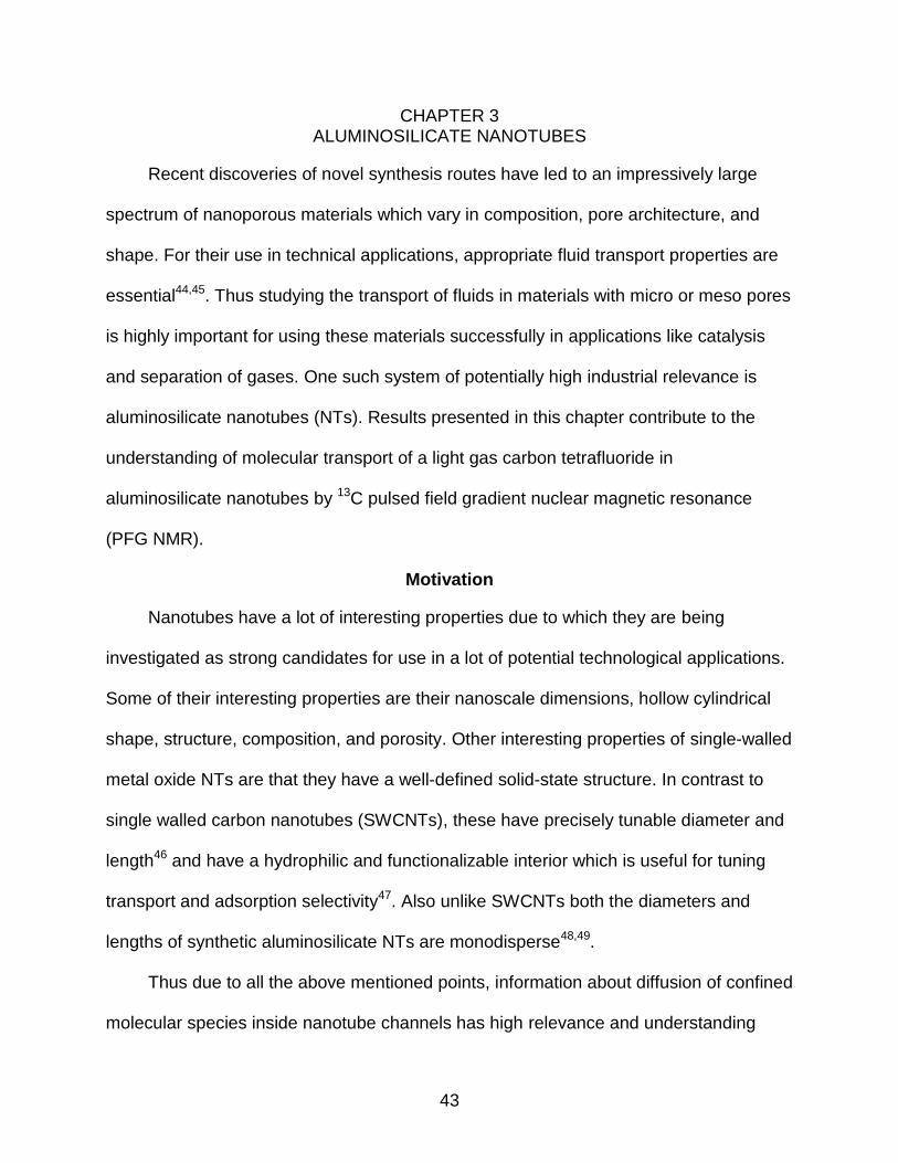
CHAPTER 3 ALUMINOSILICATE NANOTUBES
Recent discoveries of novel synthesis routes have led to an impressively large
spectrum of nanoporous materials which vary in composition, pore architecture, and
shape. For their use in technical applications, appropriate fluid transport properties are
essential44,45. Thus studying the transport of fluids in materials with micro or meso pores
is highly important for using these materials successfully in applications like catalysis
and separation of gases. One such system of potentially high industrial relevance is
aluminosilicate nanotubes (NTs). Results presented in this chapter contribute to the
understanding of molecular transport of a light gas carbon tetrafluoride in
aluminosilicate nanotubes by 13C pulsed field gradient nuclear magnetic resonance
(PFG NMR).
Motivation
Nanotubes have a lot of interesting properties due to which they are being
investigated as strong candidates for use in a lot of potential technological applications.
Some of their interesting properties are their nanoscale dimensions, hollow cylindrical
shape, structure, composition, and porosity. Other interesting properties of single-walled
metal oxide NTs are that they have a well-defined solid-state structure. In contrast to
single walled carbon nanotubes (SWCNTs), these have precisely tunable diameter and
length46 and have a hydrophilic and functionalizable interior which is useful for tuning
transport and adsorption selectivity47. Also unlike SWCNTs both the diameters and
lengths of synthetic aluminosilicate NTs are monodisperse48,49.
Thus due to all the above mentioned points, information about diffusion of confined
molecular species inside nanotube channels has high relevance and understanding
44
transport phenomena of fluids through NTs is very important in order to be able to use
these for potential applications such as catalysis, separations, molecular sensors and
encapsulation media for molecule storage, etc. Studies of transport in one-dimensional
channels are also of high interest because of the possibility of an observation of the
unique “single-file” type of diffusion50.
In this work, the potential of 13C pulsed field gradient (PFG) NMR at high magnetic
field and high magnetic field gradients for investigations of transport of adsorbed gas
molecules in novel aluminosilicate nanotubes is discussed.
PFG NMR Experiment Details
Sample Preparations
The aluminosilicate nanotubes used in this work have an outer diameter of around
2.2 nm and inner diameter of around 1.0 nm. As shown in the scanning electron
microscope (SEM) images of the studied aluminosilicate nanotubes (Figure 3-1), these
are packed into bundles forming sandwich like structures. The size ranges from half a
micrometer to few tens of micrometers.
Single-walled aluminosilicate nanotubes were synthesized according to the
protocol given in references51,52. To prepare the samples, around 150 mg of the
nanotubes was placed into a 5 mm medium walled NMR tube. The sample was
evacuated to remove any moisture present by keeping it under high vacuum (10-4 mbar)
at 453 K for 24 hours. Following the sample activation, a fixed amount of 13C-labelled
CF4 was cryogenically transferred into the NMR tube containing the sample. The tube
was then flame sealed and separated from the vacuum system. After equilibrium at 298
K the resulting gas pressure inside the tube for the sample studied was estimated to be
around 8 bars.
45
Figure 3-1. SEM images of aluminosilicate SWNT bundles. The white scale bars represent 10 µm (left) and 1 µm (right).
PFG NMR Measurements
Diffusion measurements were performed using the 17.6 T Bruker BioSpin NMR
spectrometer equipped with the Diff60 probe and Great-60 gradient amplifier (Bruker
BioSpin). The measurements were performed at a 13C resonance frequency of 188.6
MHz. The pulse sequence used for the diffusion studies was the stimulated echo pulse
sequence with the longitudinal eddy current delay (PGSTE LED)53. Attenuation curves
were plotted to study the dependence of the PFG NMR signal intensity (obtained by
integrating the area under the single line of the 13C NMR spectrum of
tetrafluoromethane) on the amplitude of the magnetic field gradient.
For molecules confined in nanopores, the proton T2 NMR relaxation times are
generally very short. This is because intra-molecular and inter-molecular dipole-dipole
interactions are not completely averaged out by molecular motion and magnetic
susceptibility. Thus for this work, 13C PFG NMR was employed instead of 1H PFG NMR
46
to take advantage of the longer 13C T2 relaxation times that are typically observed for
guest molecules confined in nanopores.
Experimental Results and their Discussion
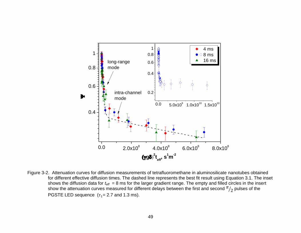
Figure 3-2 shows the 13C PFG NMR attenuation curves for diffusion of CF4 in the
studied nanotube sample at 298 K. The attenuation curves are plotted for three different
effective diffusion times ( ) i.e., 4, 8 and 16 ms. PFG NMR measurements for
effective diffusion times greater than 16 ms could not be done because of considerable
decrease in the CF4 signal due to T1 NMR relaxation for high diffusion times. In the
curves shown, the contribution from the CF4 diffusion in the gas phase (above the bed
of nanotube bundles) is subtracted. This was done by determining the bulk gas phase
contributions in separate experiments performed on an NMR tube containing only CF4
gas at a comparable pressure.
As already discussed earlier, in the case of unrestricted and isotropic diffusion,
PFG NMR attenuation curves are expected to follow a mono-exponential behaviour
given by the Equation 1.25. However, in the present case the diffusion is restricted to
one-dimensional channels that are randomly oriented. Hence isotropic 3-dimensional
diffusion cannot be expected for such a system. Consequently, the attenuation curves in
Figure.3-2 show significant deviations from the monoexponential behaviour.
In the studied sample, there are many nanotubes (or nanotube bundles) present
that are shorter ( ) than the distances travelled by the molecules during the
observation time. Due to this reason, in addition to intra-channel diffusion, it is expected
that there is an ensemble of CF4 molecules diffusing according to the mechanism of
long-range diffusion. Under the conditions of the long-range diffusion there is fast
47
exchange54 between the interiors of the nanotubes and the gas phase surrounding the
nanotubes or (nanotube bundles). Hence, the attenuation curve is expected to contain
two terms with contributions from both the diffusion mechanisms i.e., intra-channel as
well as long-range
(3.1)
where is the fraction of molecules that undergo long-range diffusion with the
diffusion coefficient being and represents the fraction of adsorbed molecules
that never leave the tubes during the observation time.
For intra-channel diffusion within randomly oriented one-dimensional channels,
the attenuation function , can be expressed as follows55
(3.2)
Equation 3.2 results in the following expression
(3.3)
where and are the diffusivities along the directions parallel and perpendicular to
the channel axis, respectively.
The dashed line in Figure 3-2 is a fit obtained by using Equation 3.1. It was found
that Equation 3.1 can be used to obtain good fits to all of the experimental data. Figure
3-3 presents the diffusion attenuation curve extended to larger gradients for effective
diffusion time of 4 ms. The dashed red curve shows the best fit using Equation 3.1, and
for comparison the result of the double-exponential fit is also shown (blue solid line).
48
For all three diffusion times used, the corresponding best fit parameters were
found to be the same within the limits of experimental uncertainty. The values obtained
for these parameters were ,
and . The Einstein relation (Equation 1.9) was used to find the
limiting values of the root mean square displacements for diffusion inside the nanotubes
and these values were estimated to be approximately 4 µm for 4 ms and 8 µm for 16
ms. These results are consistent with the observation of many sufficiently large (>10
µm) nanotube bundles in the studied sample (Figure 3-1). The presence of large
nanotube bundles proves that it is possible for the molecules to cover distances of up to
8 µm without leaving a nanotube channel.
49
0.0 2.0x10⁸
4.0x10⁸
6.0x10⁸
8.0x10⁸
0.4
0.6
0.8
1
0.0 5.0x10⁹
1.0x10¹⁰
1.5x10¹⁰
0.2
0.4
0.6
0.8
1 4 ms
8 ms
16 ms
intra-channel
mode
g2teff
, s1m
-2
long-range
mode
Figure 3-2. Attenuation curves for diffusion measurements of tetrafluoromethane in aluminosilicate nanotubes obtained for different effective diffusion times. The dashed line represents the best fit result using Equation 3.1. The inset shows the diffusion data for teff = 8 ms for the larger gradient range. The empty and filled circles in the insert
show the attenuation curves measured for different delays between the first and second pulses of the
PGSTE LED sequence ( = 2.7 and 1.3 ms).
50
0.0 5.0x10⁹
1.0x10¹⁰
1.5x10¹⁰
10-2
10-1
100
(g2teff
, s1m
-2
Figure 3-3. PFG NMR attenuations for tetrafluoromethane in aluminosilicate nanotubes at effective diffusion time of 4 ms extended to larger gradients. The dashed red curve shows the best fit using Equation 3-1. For comparison, the result of the double-exponential fit is shown (blue solid line). The empty and filled diamonds in the figure show the attenuation curves measured for different delays between the first and second pulses of the PGSTE LED sequence
( = 2.7 and 1.3 ms).
Another important result indicated by the data obtained is that the intra-channel
diffusivity remains independent of diffusion time within the limits of experimental error.
Thus it can be concluded that the measured intra-channel diffusivity is not significantly
affected by possible transport restrictions at the channel margin, i.e. it represents the
true intra-channel diffusivity. Also, the observed independence of the value of on
diffusion time for the studied range of can be explained by the existence of a broad
distribution of nanotube bundle lengths. The diffusivity along the direction of the
channels was found to be at least 4 orders of magnitude larger than that in the direction
51
perpendicular to the channels, indicating that the density of defects that would allow
diffusion of CF4 molecules in the direction perpendicular to the channel direction is
negligible.
In order to rule out possible influence of magnetic susceptibility effects on the
measured diffusion data, additional PFG NMR measurements were performed for the
same effective diffusion time (teff = 8 ms) but with different values of the delays between
the first and second pulses of the used sequence ( = 2.7 and 1.3 ms). The
observed coincidence of the PFG NMR attenuation curves measured for different
values of confirms that susceptibility effects are negligible under our measurement
conditions56.
Conclusions
13C PFG NMR at high field and high gradients was used to study diffusion of
tetrafluoromethane in novel aluminosilicate nanotubes. The data provide evidence for
one dimensional diffusion within non-intersecting channels. The measured PFG NMR
diffusion data yielded the self-diffusion coefficient of CF4 along the channel direction in
the nanotube interior as well as the corresponding diffusivity of CF4 molecules
undergoing fast exchange between many nanotubes. The intra-channel diffusivity was
found to remain independent of diffusion time within the limits of experimental error.
52
LIST OF REFERENCES
(1) Fick, A. E. Ann. Phys. 1855, 94, 59.
(2) Fick, A. E. Phil. Mag. 1855, 10, 30.
(3) Crank, J. The Mathematics of Diffusion; Claredon Press: Oxford, 1975.
(4) Kärger, J.; Vasenkov, S.; Auerbach, S. M. Diffusion in Zeolites. In Handbook of Zeolite Science and Technology; Auerbach, S. M., Carrado, K. A., Dutta, P. K., Eds.; Marcel Dekker, Inc.: New York, Basel, 2003; pp 341.
(6) Kärger, J.; Pfeifer, H.; Heink, W. Advances in Magnetic Resonance; Academic Press: New York, 1988.
(7) Kärger, J.; Ruthven, D. M. Diffusion in Zeolites and Other Microporous Solids; Wiley & Sons: New York, 1992.
(8) Levitt, M. H. Spin dynamics : basics of nuclear magnetic resonance, 2nd ed.; John Wiley & Sons: Chichester, England ; Hoboken, NJ, 2008.
(9) Keeler, J. Understanding NMR spectroscopy, 2nd ed.; John Wiley and Sons: Chichester, 2010.
(10) Callaghan, P. T. Principles of nuclear magnetic resonance microscopy; Clarendon Press Oxford University Press: Oxford England New York, 1991.
(11) Gibbs, S. J.; Johnson, C. S. Journal of Magnetic Resonance (1969) 1991, 93, 395.
(12) Cotts, R. M.; Hoch, M. J. R.; Sun, T.; Markert, J. T. J. Magn. Reson. 1989, 83, 252.
(13) Galvosas, P.; Stallmach, F.; Seiffert, G.; Kärger, J.; Kaess, U.; Majer, G. J. Magn. Reson. 2001, 151, 260.
(14) Wu, D. H.; Chen, A. D.; Johnson, C. S. Journal of Magnetic Resonance, Series A 1995, 115, 260.
(15) Wider, G.; Dotsch, V.; Wuthrich, K. Journal of Magnetic Resonance, Series A 1994, 108, 255.
(16) Levitt, M. H.; Forsterling, F. H. Medical Physics 2010, 37, 406.
(17) Price, W. S. Concepts in Magnetic Resonance 1997, 9, 299.
53
(18) Lee, B. C.; Outcalt, S. L. Journal of Chemical & Engineering Data 2006, 51, 892.
(19) Dzyuba, S. V.; Bartsch, R. A. ChemPhysChem 2002, 3, 161.
(20) Brennecke, J. F.; Maginn, E. J. AIChE Journal 2001, 47, 2384.
(21) Swatloski, R. P.; Visser, A. E.; Reichert, W. M.; Broker, G. A.; Farina, L. M.; Holbrey, J. D.; Rogers, R. D. Green Chem. 2001, 4, 81.
(22) Visser, A. E.; Swatloski, R. P.; Reichert, W. M.; Mayton, R.; Sheff, S.; Wierzbicki, A.; Davis Jr, J. H.; Rogers, R. D. Chem. Commun. 2001, 135.
(23) Merrigan, T. L.; Bates, E. D.; Dorman, S. C.; Davis Jr, J. H. Chemical Communications 2000, 2051.
(24) Welton, T. Chem. Rev. 1999, 99, 2071.
(25) Blanchard, L. A.; Hancu, D.; Beckman, E. J.; Brennecke, J. F. Nature 1999, 399, 28.
(26) Scurto, A. M.; Aki, S. N. V. K.; Brennecke, J. F. Journal of the American Chemical Society 2002, 124, 10276.
(27) Dupont, J.; de Souza, R. F.; Suarez, P. A. Z. Chemical Reviews 2002, 102, 3667.
(28) Wasserscheid, P.; Keim, W. Angewandte Chemie International Edition 2000, 39, 3772.
(29) Sheldon, R. Chem. Commun. 2001, 2399.
(30) Quinn, B. M.; Ding, Z.; Moulton, R.; Bard, A. J. Langmuir 2002, 18, 1734.
(31) Kim, K.; Lang, C.; Moulton, R.; Kohl, P. A. Journal of the Electrochemical Society 2004, 151, A1168.
(32) Wu, B.; Reddy, R. G.; Rogers, R. D. “Novel Ionic Liquid Thermal Storage for Solar Thermal Electric Power Systems”; Proceeding of Solar Forum, 2001, Washington, DC.
(33) Chiappe, C.; Pieraccini. D. Journal of Physical Organic Chemistry 2005, 18, 275.
(34) DeSimone, J. M. Science 2002, 297, 799.
(35) Pez, G. P.; Carlin, R. T.; Laciak, D. V.; Sorensen, J. C. Method for gas separation; Google Patents, 1988.
54
(36) Lee, B.-C.; Outcalt, S. L. Journal of Chemical & Engineering Data 2006, 51, 892.
(37) Bates, E. D.; Mayton, R. D.; Ntai, I.; Davis, J. H. J. J. Am. Chem. Soc. 2002, 124, 926.
(38) Husson-Borg, P.; Majer, V.; F., C. G. M. J. Chem. Eng. Data 2003, 48, 480.
(39) Baltus, R. E.; Culbertson, B. H.; Dai, S.; Luo, H. M.; De Paoli, D. W. L. J. Phys. Chem. B 2004, 108, 721.
(40) Shiflett, M. B.; Yokozeki, A. Ind. Eng. Chem. Res. 2005, 44, 4453.
(41) Jalili, A. H.; Mehdizadeh, A.; Shokouhi, M.; Ahmadi, A. N.; Hosseini-Jenab, M.; Fateminassab, F. The Journal of Chemical Thermodynamics 2010, 42, 1298.
(43) Hou, Y.; Baltus, R. E. Ind. Eng. Chem. Res. 2007, 46, 8166.
(44) Barton, T. J.; Lucy, M.; Klemperer, W. G.; Loy, D. A.; McEnaney, B.; Misono, M.; Monson, P. A.; Pez, G.; Scherer, G. W.; Vartuli, J. C. Chemistry of materials 1999, 11, 2633.
(45) Selvam, P.; Bhatia, S. K.; Sonwane, C. G. Industrial & engineering chemistry research 2001, 40, 3237.
(46) Konduri, S.; Tong, H. M.; Chempath, S.; Nair, S. The Journal of Physical Chemistry C 2008, 112, 15367.
(47) Zang, J.; Konduri, S.; Nair, S.; Sholl, D. S. ACS nano 2009, 3, 1548.
(48) Mukherjee, S.; Bartlow, V. M.; Nair, S. Chemistry of materials 2005, 17, 4900.
(49) Mukherjee, S.; Kim, K.; Nair, S. Journal of the American Chemical Society 2007, 129, 6820.