55
Reforming Agricultural Subsidies for Improved Environmental Outcomes by Abdullah Mamun, Will Martin, Simla Tokgoz International Food Policy Research Institute 6 September 2019

Reforming Agricultural Subsidies for Improved Environmental Outcomes
by
Abdullah Mamun, Will Martin, Simla Tokgoz
International Food Policy Research Institute
6 September 2019

Executive Summary
Does agricultural support contribute to environmental degradation?
Agricultural production and land use change leave a significant environmental footprint. They are
responsible for roughly a quarter of global greenhouse gas (GHG) emissions. Support measures
promoting agricultural production with existing technologies therefore likely contribute to
environmental degradation and climate change. However, assessing the impact is not
straightforward, as environmental outcomes depend on how agricultural policies influence the mix
of goods produced and how those goods are produced. The present study addresses two key
questions in this context: (i) what are the implications of existing support measures for agricultural
output and emissions? and (ii) how might these support measures be repurposed to help improve
environmental, social, and nutritional outcomes?
Governments provide near US$600 billion in agricultural subsidies every year
Globally, agricultural support is very substantial, with farmers in 51 key countries receiving
US$483 billion per year between 2015 and 2017, enough to raise their returns by 18 percent on
average. The same set of countries spent US$86 billion per year on public goods that create
enabling conditions for agriculture, such as agricultural innovation systems and rural
infrastructure. Given the extremely high returns estimated for these public goods, governments
could well over-invest in farm-level support and under-invest in providing public goods that could
both contribute to food security and to agriculture’s contribution to climate change mitigation and
adaptation.
Some forms of support distort agricultural markets more than others
Agricultural support can divided into three types: (i) trade or border measures such as tariffs or
quotas that provide market price support (MPS); (ii) coupled subsidies (CS) provided by
governments as direct subsidies on output or as subsidies on inputs (such as fertilizers or seeds)
that create incentives to increase output; and (iii) decoupled subsidies (DS) that avoid altering
incentives to change output levels but provide direct income support to farmers.

ii
In the trade context, there is a clear ranking of these measures, with market price support
being the most distorting, because it simultaneously increases supply and reduces demand.
Coupled subsidies are generally less distorting because they affect only supply, while decoupled
subsidies are least distorting because, at least in principle, they are meant to affect neither supply
nor demand. This ranking is much less clear when the focus is on the impact on GHG emissions.
For instance, market price support through trade policies creates a stronger incentive to reduce
output in trade competing countries, than would be the case for coupled subsidies.
The nature of agricultural support has changed substantially
The traditional pattern of agricultural support involved substantial support to farmers in the rich
countries, while poor countries, on balance, used to tax agriculture. This pattern has changed
substantially over the past decades (see Figure A).
Figure A. Nominal rates of assistance by type of support
Note: Support is expressed as a % of value of production at undistorted prices.
In wealthy nations, average rates have fallen and there has been a move away from trade
measures and towards decoupled protection that seeks to avoid pushing for higher agricultural
production and reducing the market access opportunities of other countries. In developing
countries, agricultural support has shifted from net taxation to net assistance on average.
Nowadays, most support is provided through border measures that generate revenues, such as
tariffs, rather than subsidies paid by governments.
0
10
20
30
40
50
60
70
80
1991 1996 2001 2006 2011 2016
No
min
al r
ate
of
asis
tan
ce (
%)
OECD
-20
-10
0
10
20
30
40
50
60
70
80
1993 1998 2003 2008 2013
Non-OECD
Market Price Support
Coupled Subsidies
Decoupled Subsidies
Total Support

iii
Since market price support rarely requires budgetary funding, it usually does not face the
same scrutiny as output or input subsidies. Both coupled and decoupled subsidies tend to face
greater scrutiny because governments must allocate funds to these subsidies. Overall, most
support to world agriculture is provided through market price support, rather than subsidies.
GHG emissions from agriculture are strongly concentrated by product
How does the present regime of agricultural support impact on the environment and on GHG
emissions, in particular? To assess this, it is important to note that at present GHG emissions are
strongly concentrated by product. Ruminant meat, milk and rice production account for more
than 80 percent of agricultural emissions, with ruminant meat alone accounting for half of these
in both OECD and developing countries. Milk and ruminant meats are roughly twice as
emission-intensive in poorer countries than in today’s OECD countries—a difference that is
strongly related to differences in productivity. At the same time, however, agricultural emission
intensities (emissions per unit of output) have been falling much more rapidly in non-OECD
countries than in OECD countries. This is fortunate given that agricultural production has been
growing much more rapidly in the developing world (2.6 percent per year vs 0.5 percent per year
in developed countries). As a result, the share of developing countries in global emissions from
agricultural production has remained close to that reached in 1991 (74 percent).
Land use and land use change also contribute substantially to global emissions.
Deforestation is the most important of the related emissions and much of which – in turn –is
driven by expansion of production of emission-intensive commodities, such as livestock
products. While forests in the OECD countries and in most of Asia reduce atmospheric CO2 by
converting it through photosynthesis, there are substantial net emissions from deforestation in
South America, South East Asia, and Africa.
Agricultural policies are more-or-less neutral in supporting high emission-intensive vis-à-vis
low emission-intensive products
Agricultural support increases global agricultural output by increasing its profitability, although
this effect is likely quite small as increases in overall output require producers either to draw new
land into agriculture or to substitute other inputs (such as fertilizers) for land. As a first, simple
approach one can assess the likely impact of agricultural subsidies by identifying whether the

iv
support is biased towards emission-intensive products or not. In the early 1990s, this bias appears
generally to have been away from emission-intensive goods. On average for the world, this bias
was essentially non-existent by 2015.
How to realign agricultural subsidies?
Given the importance of emissions from agriculture and land use change, measures to mitigate
them are almost certainly needed if effective reductions in global emissions are to be achieved.
This is particularly the case given that demand for the most emission-intensive goods—red meat
and dairy products—is likely to increase more rapidly than demand for staple foods because of
income growth in developing countries and increase in rate of urbanization.
Policy reform will be challenging given the strong political support for the current
system. Experience suggests that focusing on a narrow reform agenda is particularly difficult
because the interested parties in such a discussion are those who would lose from abolition of
this support. To increase the chances of success, reformers need to make a careful strategic
decision about the breadth of the policy agenda, including measures that would generate benefits
to key interest groups. The Uruguay Round of trade negotiations is an important example of an
extremely broad agenda that succeeded—by bringing in additional interest groups, such as those
focused on trade in services—in introducing massive reforms in agricultural incentives.
However, there is an optimal span of topics for reform advocacy and/or negotiation because
greater breadth also increases the complexity of communicating results and potentially the
challenges of reaching agreement.
Another key question relates to the geographic focus of reform efforts. The global nature
of the GHG problem suggests a global effort is needed, but many of the policies that influence
global outcomes are determined at national or sub-national levels, where governance
mechanisms are much more strongly developed. Reaching effective agreements at the global
level has proved difficult, but such agreements have the advantage of allowing governments to
make lasting commitments for reform.

v
Support should shift from the farm to public goods
Given the vast support currently being provided to farmers, there are clearly many potential
approaches that might be used to achieve better economic, environmental and nutritional
outcomes. From the available evidence it seems likely that such reform packages would include
investments in R&D to raise productivity, reduce emissions reduce the long-run agricultural land
use footprint and particularly the adverse impacts of deforestation; realignments in support to
raise efficiency and reduce emissions; and incentives to improve nutritional outcomes in high-
income countries.
However, successful policy reform is not brought about simply by identifying such policy
packages. Successful reform advocacy tends to combine analysis focused on identifying policy
challenges and reforms, and coalition building focused on achieving reforms. A key question is
which interest groups might engage on reform of agricultural subsidies in the future. Reformers
need to develop a reform narrative that frames the issues in a way that makes the benefits of
reform clear and mobilizes a range of actors in support of a specific approach to reform.
Discourse coalitions can help build such a shared understanding and identify narratives that will
convey its essence to broader groups of stakeholders. While the road to such reform is likely to
be long and hard there is, at last, a great deal of attention focused on how this might be done.

* We wish to thank Lars Brink, Shenggen Fan, Joe Glauber, Thom Jayne, David Laborde, Rob Vos and participants
in seminars at IFPRI and the Meridian Institute for valuable comments. We alone are responsible for all remaining
errors.
I. Introduction*
The fifty-one developed and developing countries covered by the OECD’s 2018 agricultural
policy monitoring and evaluation provided $483 billion per year in 2015-17 in support to farmers
(OECD 2018, p105) and an additional $86 billion on services such as agricultural innovation,
infrastructure and stockholding. Most of the $483 billion in support is provided by trade
measures that raise (or lower) the prices received by farmers relative to world prices, with the
remainder provided by subsidies. While agriculture has many environmental impacts, we focus
on emissions of greenhouse gases (GHG) because of their global impact and their potentially
catastrophic consequences for the world, and for agriculture in particular. With agricultural
production and land use change contributing close to a quarter of global GHG emissions, this
spending has potentially large implications for greenhouse gas emissions and hence for climate
change. However, the magnitude and even the direction of these policy impacts is uncertain,
making analysis essential for well-founded policy recommendations.
These incentives affect environmental outcomes by changing (i) how much is produced,
(ii) what is produced, (iii) where it is produced, and (iv) how goods are produced. To assess the
environmental impact of agricultural subsidies, we need to account for the output-related effects
((i), (ii) and (iii)) and the technology effects (iv). Support that is coupled with output of
emission-intensive goods generally increases output in the subsidizing region and the associated
emissions. Use of coupled support will be particularly damaging for global emissions if the
emission intensity (emissions per unit of output) is higher in the region providing support than in
other regions, or if it encourages the use of emission-intensive practices or technologies.
Similarly, support coupled with specific inputs will encourage excessive use of those inputs and
may generate increased emissions if the input is emission-intensive. Decoupled support, by
contrast, is expected to transfer revenues directly to recipients without altering market incentives,
potentially reducing economic and environmental costs and providing greater net benefits to
producers per dollar of support.
Support to farmers may also have favorable impacts on environmental outcomes. If, for
instance, support is provided primarily for products that are relatively less emission-intensive, it
may take resources away from emission-intensive activities. If support is provided subject to
conditions designed to improve environmental outcomes it may also help to reduce emissions.

2
Support may also be designed to create incentives for producers to use Climate Smart production
approaches that both reduce costs and contribute to better environmental outcomes (Engel and
Muller 2015) or to help the agricultural sector to adapt to climate change (Glauber 2018).
Policy makers have many goals for agriculture—including achieving food security,
generating incomes for farmers, and rectifying market failures such as environmental
externalities and the lack of incentive for individual farmers to invest in research and
development. To achieve these targets, policy makers must have at least as many policy
instruments as they have goals (Tinbergen 1956). Fortunately, policy makers have many policy
instruments including different types of agricultural subsidies and measures affecting emissions
and nutritional outcomes more directly. Widely-used measures with important impacts on
agriculture include: (i) provision of public goods such as rural infrastructure, agricultural
research and development, and water rights, (ii) consumer taxes or subsidies that influence the
demand for agricultural products without being directly identified as producer subsidies or taxes,
(iii) policies affecting demand and supply in downstream value chains of agricultural
commodities (eg biofuel policies1). Considering the full range of relevant policies is important
not just for achieving the goals of any individual policy maker, but also for helping reach
agreement on policy reforms, especially where different stakeholders have sharply different
interests and/or preferences.
Many critiques of current agricultural subsidies—and agricultural policies more
generally—have pointed to contradictions at the heart of current policies. Most support is
provided in the form of higher prices or direct subsidies that create deadweight economic losses,
provide most of their benefits to larger producers, and are capitalized into land values (Goodwin
et al. 2012), while policymakers frequently under-invest in public goods such as research,
innovation and infrastructure. Support varies widely by commodity and is frequently lavished on
foods that are particularly large sources of greenhouse gases. Towering subsidies in rich
countries frequently deny poor farmers in developing countries the opportunity to compete.
Many people remain unable to access enough food because they are too poor to be able to buy
food. At the same time, the diets of many others include excessive quantities of fat, meat and
1 Which may be provided indirectly through mandates or regulations on fuel use or through exemptions from duties
otherwise levied on fuel use and are not considered in the OECD measures of agricultural support.
3
sugar, which have contributed to an epidemic of non-communicable diseases such as diabetes
(Masters et al. 2015). Many critiques are available (eg Tilman and Clark 2014; Springmann et al.
2017; Willet et al. 2019), but few plans for concrete action to improve the situation.
In the next section of the paper, we consider the range of policy instruments used to
influence agricultural outcomes and the extent to which they change farmers’ incentives to
produce. In the third section we focus on the greenhouse gas emissions associated with
agriculture and land use change. Then, in the fourth section, we consider the potential impacts of
subsidies and related measures on emissions. The fifth section examines policy conditionality
and targeting. With this as backdrop, the sixth section considers potential paths to reform, given
political-economy constraints on and opportunities for reform. Conclusions are presented in
section VIII.
II. Agricultural Subsidies and Related Measures
Support to (and taxation of) agriculture comes in many forms, but it is useful to distinguish three
main forms of support2: (i) Market price support, (ii) Coupled subsidies, and (iii) Decoupled
subsidies. Governments generate market price support by introducing barriers to trade such as
tariffs, licenses and quotas that raise (or lower) the domestic price relative to world prices.
Coupled subsidies include measures such as subsidies to output or to inputs that increase the
returns to producers and hence their incentives to produce specific goods. Decoupled subsidies
base payments on something fixed, such as production in an historical period and remove the
link between support and output levels. In addition to the support provided in the form of
subsidies, governments also intervene to improve the enabling environment for agriculture,
providing goods that would otherwise be under-provided, such as research and development and
rural infrastructure. Governments also intervene in many ways that indirectly affect agriculture,
but outside the scope of support as conventionally defined, such as by imposing mandates for use
of biofuels and improving access of poor people to food through social safety net programs.
2 Throughout this study, we build on the OECD measures of agricultural incentives. Market Price Support is defined
as in the OECD PSE Manual (OECD 2016). Coupled subsidies refers to the budgetary transfers and revenue
foregone due to measures specific to agriculture, administered in ways that create incentives to change output levels.
Decoupled subsidies are measures intended to avoid creating incentives to change output, specifically categories E
(production not required); F (Payments based on non-commodity criteria) and G (miscellaneous payments) of the
OECD (2016, p23)

4
These forms of support differ in two important ways—whether governments need to fund
them directly, and how they influence production. Market price support is generally found in
importing countries, where the fact that tariffs raise revenue makes it attractive to policy makers
and reduces the need for (frequently rigorous) review by Ministries of Finance. Subsidies, by
contrast, need to be funded from scarce government resources and so tend to undergo regular
scrutiny. Market price support distorts both consumption and production decisions, while
coupled subsidies directly distort only production.
Historically, developed countries have tended to subsidize agriculture, frequently using
trade barriers to reduce imports. Developing countries frequently used export taxes to lower
domestic prices, lowering food costs to the frequently more politically powerful consumer group,
and lowering returns to producers. Developing countries also saw the agricultural sector as a
source of government revenue, taxing export commodities, especially cash crops. Developed
countries frequently provided coupled subsidies in addition to market price support. Some
developing countries also use coupled subsidies measures, sometimes to offset the adverse
impacts of export taxes on farmer incentives. As shown by Anderson (1995), there were strong
political-economy reasons for poor countries to tax agriculture while rich countries protected it.
Historically, few countries used decoupled support, although it does allow governments to
transfer resources to producers without the costly side effect of stimulating production that costs
more than its value to society.
Figure 1 presents the average nominal rate of protection (NRP) for agriculture for high-
income and developing countries, underlining the above discussion. The NRP reflects the
support provided by border measures such as tariffs and quotas, or taxation imposed through
measures like export taxes or quotas. NRPs in high-income countries rose until the late 1980s
and have since declined. NRPs in developing countries were negative until the early 1990s but
have since become modestly positive on average.
As protection to agriculture in the industrial countries rose in the 1970s and 1980s
(Figure 1), it created increasing conflict between countries, with exporters dismayed by the low
prices that ensued when other exporters paid substantial export subsidies—and the subsidizers
realizing that their expensive subsidies were depressing world prices rather than achieving their
desired goal of raising producer prices (Johnson 1991). Reforming these policies was

5
challenging, and required a sustained push from policy reformers, accompanied by policy
analysis identifying options for reform and analyzing their consequences. During the Uruguay
Round, WTO members identified approaches that would allow them to begin the process of
reducing support provided through border measures (Martin and Winters 1996).
Figure 1. Nominal Rates of Protection in High Income and Developing Countries, %
Sources: 1955–2004, Anderson (2009); 2005–2014, Ag Incentives Consortium, www.ag-incentives.org.
While the restrictions on industrial country support to agriculture under the Uruguay Round were
weaker than they seemed (Hathaway and Ingco 1995), they appear to have had an enormous
impact on applied rates of agricultural protection. After rising continuously between the 1950s
and the late 1980s—except for a sharp decline during the 1973-4 commodity boom—border
support in the industrial countries fell sharply from the early 1990s. In the developing countries,
the limits on agricultural support were much weaker relative to prior levels of support, and the
sharp upturn in economic growth rates of developing countries beginning in the early 1990s
contributed to an increase in border protection from the consistently-negative rates prior to the
1990s to slightly positive-on-average assistance since that time (Martin 2018a).
While there are many ways we could split the protection data geographically, we focus
primarily on the distinction between the generally-higher-income OECD countries and the non-
OECD countries. We do this to investigate the differences in the overall emission intensity and
-40
-20
0
20
40
60
80
%
HIC DCs
6
emission levels in these groups of countries. We also consider this split because of the sharp
differences in patterns of support between these two groups. Supplementary data for several key
countries is given in the appendix.
The WTO limits on market price support are commodity-specific while those on
domestic subsidies include flexibility to average across many commodities. Decoupled subsidies
are, by design, essentially unconstrained by WTO rules. These rules might be expected to result
in a shift in support away from market price support. To see whether this has been the case, we
compare the evolution of these three different forms of support in Figure 2. For this analysis, we
turn to the OECD database that covers 85 percent3 of global agricultural production (12 non-
OECD and almost all OECD economies) and allows us to disaggregate protection measures in
the way that we need, although its coverage of smaller developing countries is less than in the
broader Ag Incentives database4 underlying Figure 1.
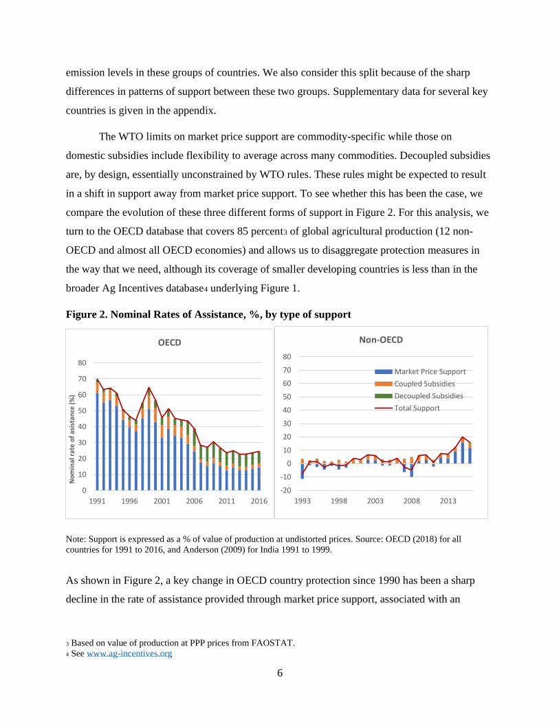
Figure 2. Nominal Rates of Assistance, %, by type of support
Note: Support is expressed as a % of value of production at undistorted prices. Source: OECD (2018) for all
countries for 1991 to 2016, and Anderson (2009) for India 1991 to 1999.
As shown in Figure 2, a key change in OECD country protection since 1990 has been a sharp
decline in the rate of assistance provided through market price support, associated with an
3 Based on value of production at PPP prices from FAOSTAT.
4 See www.ag-incentives.org
0
10
20
30
40
50
60
70
80
1991 1996 2001 2006 2011 2016
No
min
al r
ate
of
asis
tan
ce (
%)
OECD
-20
-10
0
10
20
30
40
50
60
70
80
1993 1998 2003 2008 2013
Non-OECD
Market Price Support
Coupled Subsidies
Decoupled Subsidies
Total Support
7
increase in decoupled subsidies. Market Price Support in the OECD countries fell from over 60
percent in 1991 to 13 percent in 2016, computed as market price support in share of agricultural
sectors’ value of production. By contrast, decoupled support rose from only 2 percent in 2006 to
a peak of 11 percent in 2006, declining to 8 percent in 2016, as a share of agricultural production
value. Distorting coupled subsidies such as output and input subsidies declined from almost 7
percent of agricultural production value in 1991 to 2.6 percent in 2016. However, market price
support has risen slightly in recent years, suggesting a continuing tendency for support to rise
when world prices fall.
In non-OECD countries, total support was much more volatile, being negative in the
early 1990s and around the 2007-2008 price spike and oscillating around zero in most years up to
2013. However, between 2014 and 2016, it increased dramatically, peaking at 19.9 percent of the
value of production at undistorted prices in 2015. Most of the support in non-OECD countries is
in the market price support category and decoupled subsidies remain very small. Coupled
subsidies, such as those on output and on inputs such as fertilizer and water, accounted for about
a quarter of total support in 2016
To understand developments in OECD countries’ support to agriculture, it’s important to
look at the two largest players, the European Union (EU28) and the United States, as shown in
Figure 3. In the European Union, support was almost exclusively provided by market price
support in 1990, with only 2.7 percentage points of the 87.6 percent support provided by
decoupled payments. From the early 2000s, however, decoupled subsidies began to replace
coupled subsidies, with both market price support and coupled subsidies dropping dramatically
as a share of the value of output, while decoupled subsidies rose sharply in importance. By 2016,
decoupled subsidies accounted for 15 percent out of 25 percent in total support. In the United
States, both the share and the level of market price support fell sharply over the period. Both
coupled and decoupled subsidies rose dramatically during the period of depressed world prices
beginning in 1998. By 2016, total support, at 9 percent, was less than half the level in 1991 and
decoupled support made up close to half of that support.

8
Figure 3. Nominal Rates of Assistance in the EU28 and the USA, %, by type of support
Note: All measures as defined in Figure 2.
Given the size of China and India as agricultural producers, changes in average agricultural
support to non-OECD countries tend to be driven by changes in their support. In China, the
picture is very clear, with nominal rates of assistance trending up from about 2000 from the
negative levels that had prevailed in the 1980s and 1990s. While China provided some coupled
subsidies and decoupled subsidies, these were very small throughout the period relative to
market price support. Roughly half of the market price support was provided to maize, pork, rice
and wheat in 2015 (OECD 2018). Since then, market price support to maize has fallen
dramatically with the abolition of the administered price for maize (WTO 2019).
In India, market price support has been negative and substantial throughout most of the
period, although the rate of taxation on agriculture declined sharply in the last two years of the
sample. Because domestic prices are insulated from world market prices, the market price
support/taxation for individual commodities varies sharply from year to year, but the
commodities with the largest negative transfers—accounting for more than half the total negative
MPS—on average between 2005 and 2016 were milk, rice, wheat, bananas and mangoes.
Coupled subsidies, mostly in the form of input subsidies, have been positive throughout the
period but substantially below the rate of agricultural taxation leaving total assistance strongly
negative in most years.
0
20
40
60
80
100
1991 1996 2001 2006 2011 2016
No
min
al r
ate
of
assi
stan
ce (
%)
European Union
0
10
20
30
40
50
60
70
80
90
100
1991 1996 2001 2006 2011 2016
USA
Market Price Support
Coupled Subsidies
Decoupled Subsidies
Total Support

9
Figure 4. Nominal Rates of Assistance in China and India, % by type of support
The impact of agricultural subsidies on environmental externalities is influenced both by the
extent to which they increase agricultural output and the extent to which they change the mix of
products produced. Since the responsiveness of overall food demand and supply to prices are
low, output is not likely to be greatly changed by agricultural support. However, switching land
between agricultural commodities is relatively easy so the relative incentives to produce different
types of food are likely to be important.
If subsidies are substantial and linked to output of emission-intensive commodities such
as rice and livestock products, then subsidies will increase emissions from these products. The
average subsidy rate to individual commodities is shown in Figure 5 for both OECD and non-
OECD emerging economies. This measure includes only measures that support individual
commodities, either through market price support or output/input subsidies and therefore almost
entirely excludes decoupled transfers. Within the OECD, the highest rate of assistance is to rice,
followed by sugar and then a set of livestock products. For the non-OECD countries, rice, wheat,
sugar and milk all have relatively high rates of support. Within both groups of countries, there is
considerable variation across commodities.
-20
-10
0
10
20
30
40
1993 1998 2003 2008 2013
No
min
al r
ate
of
assi
stan
ce (
%)
China
Market Price Support
Coupled Subsidies
Decoupled Subsidies
Total Support
-50
-40
-30
-20
-10
0
10
20
30
1991 1996 2001 2006 2011 2016
India

10
Figure 5. Transfers to specific commodities, 2014-16, %
Note: Other SCT refers to Single Commodity Transfers other than those provided by Market Price Support. All
percentages are relative to the undistorted value of production.
Both OECD and non-OECD countries provide public goods such as agricultural research and
innovation investments and rural infrastructure. The benefit-cost ratios for these interventions
have been found to be generally substantially greater than one (Alston 2018; Fan, Cho and Rue
2018; Mogues et al. 2012), with the highest rates of return to investments in research and
development. By contrast the benefit-cost ratio for subsidies is almost by definition less than one
because of the deadweight costs associated with inducing high-cost production and distorting
consumer choices. In both country groups, public-good investments are small relative to total
support. In the OECD countries, they average around 12 percent of total support (OECD 2018),
with the largest allocations going to infrastructure and research and knowledge generation. In
the non-OECD countries, this type of support averaged around 16 percent of total support, with
the largest amount spent on public stockholding and most of the remainder on infrastructure and
knowledge generation.
0 50 100 150
Barley
Beef and veal
Eggs
Milk
Oats
Pig meat
Poultry meat
Rapeseed
Rice
Sheep meat
Sorghum
Soybeans
Sugar
Sunflower
Wheat
Wool
% ad valorem equivalent
OECD
Other SCT MPS
-40 -20 0 20 40 60
% ad valorem equivalent
Axi
s Ti
tle
Non-OECD

11
III. Emissions from Agriculture and Land Use
When considering mitigation priorities, a key question is the importance of each emission
source, simply because any given percentage reduction in emissions has a larger impact, the
larger the underlying flow of emissions. Figure 6 compares emissions from agriculture and land
use change with those from nonagricultural sources such as energy and industry, transport and
residential/commercial uses. This figure makes clear that agriculture and land use change are
major sources of emissions. With almost a quarter of global net emissions, they clearly need to
be addressed if comprehensive reductions in emissions are to be achieved. Another striking
feature of the graph is the small contribution made to emissions from international transport,
including bunkers for shipping and aviation fuel, relative to other sources of emissions.
Figure 6. Emissions by Source, 2010, %
Source: FAOSTAT. Note: The striped section of the Transport bar refers to international transport, while the striped
section of the Agric and Land Use bar refers to land use, excluding carbon sequestration by forests, which is shown
in the last bar.
-10
0
10
20
30
40
50
60
70
Energy &Industry
Transport Residential &commercial
Agric & LandUse
Forest
% o
f To
tal E
mis
sio
ns

12
In the next sub-section of this paper, we focus on the ongoing emissions from agriculture, while
in the following one we consider emissions from land use and land use change.
Emissions from Agricultural Production
Since most distortions to agricultural incentives are commodity-specific, emissions per unit of
commodity output are needed to understand the direct impact of agricultural distortions on
emissions. Fortunately, Tubiello et al. (2012 and 2013) developed such a set of measures and
estimates based on this methodology are freely downloadable from FAOSTAT (Tubiello 2019).
These estimates are based on the IPCC Tier 1 Methodology that uses relatively stylized estimates
of emissions per unit of output by region (IPCC 2006), these estimates are still sophisticated
enough to differentiate between regions based on key agro-ecological features5. While the
original database, as documented in Tubiello et al. (2013) included only rice and livestock
products, the current version also includes non-rice cereals. Tubiello et al. (2013) notes that these
GHG emission estimates cover over 80%-85% of total agricultural sector emissions, of which
majority comes from livestock (Tubiello et al. 2012). Estimates of agricultural emissions by
commodity as a share of total emissions for included sectors are presented in Table 1.
Table 1. Shares of Agricultural Emissions by Commodity, %, 2015
OECD Non-OECD World
% % %
Rice 3.4 18.8 15.5
Other Cereals 18.7 7.4 9.8
Milk 18.8 17.8 18.0
Ruminant meat 49.2 50.5 50.2
Pigmeat 7.3 3.2 4.0
Poultry meat 1.4 1.3 1.3
Eggs 1.1 1.1 1.1
Total (from included sectors) 100 100 100 Note: CO2 equivalent. Source: FAOSTAT, Accessed 2 February 2019
5 See IPCC (2006, Ch 10) for details of the attributes used to distinguish between livestock production systems in
different countries and Tubiello (2013, p5) for very specific references to the emissions factors used by product and
region. In this section, the listing of non-OECD countries is comprehensive.

13
A striking feature of Table 1 is the large share of ruminant meat (cattle, buffalo, goats and sheep)
in total emissions, both in the OECD and in the rest of the world. Another striking feature is the
enormous difference in the importance of rice between the OECD and the Non-OECD countries.
Milk production emissions accounts for around 18 percent in both regions. Pigmeat and poultry
products account for only six percent of total emissions globally, and less than 10 percent even in
the OECD countries. Close to 70 percent of emissions are associated with production of
ruminant meat and milk largely because emissions resulting from enteric fermentation in the
ruminant digestive process and emissions associated with manure are important contributors to
global emissions from agriculture (see Tubiello et al. 2013, p6). The shares of emissions from the
non-OECD group are much more relevant—and much closer to the world average shares—
because non-OECD emissions from agriculture are 3.6 times as large as those from the OECD
group.
The substantial support to milk production in both OECD and non-OECD countries is
seen in Figure 5. This and the substantial support to beef production in the OECD countries
clearly have important implications for producer incentives. The fact that most of this support is
provided through market price support is something of a mixed blessing. Market price support is
clearly worse than coupled subsidies when the focus is on trade impacts since market price
support in protecting countries increases production in these countries and lowers global prices.
However, when the focus is on global emissions, the feature that is adverse for trade, the larger
reduction in prices outside the group of protecting countries has a favorable impact. Countries
not providing protection through market price support —or providing less than the average
amount of support—face lower external market prices and reduced incentives for production
than if the same amount of producer support were provided by coupled subsidies in the
protecting country. This distinction is fundamentally important and does not appear to have been
considered in other studies. In fact, it reverses the widely used ranking of MPS and coupled
subsidies under which MPS is considered more perverse than coupled subsidies (Mayrand et al.
2003, p41). While capturing the quantitative effect of this distinction requires a formal model, it
is important to recognize it in a broad study of this type.
To the extent that market price support in OECD countries stimulates output in those
countries while depressing output in other countries, it is important to examine differences in the
emission intensity of production in each region. Table 2 reveals some striking differences in

14
emission intensities of commodities, with emissions per kg of output twice as high for ruminant
meat and more than twice as high for milk in non-OECD countries relative to the OECD. By
contrast, emissions per unit of output were substantially lower in the non-OECD countries for
rice and for pigmeat.
Table 2. Average Emission Intensities by product, kg CO2 eq/kg of output.
OECD Non-OECD World
Rice 1.1 0.9 0.9
Other Cereals 0.2 0.2 0.2
Milk 0.5 1.3 1.0
Ruminant meat 16.0 32.4 26.6
Pigmeat 1.7 1.4 1.5
Poultry meat 0.3 0.7 0.6
Eggs 0.5 0.8 0.7
Source: Authors’ calculation based on FAOSTAT data on emissions and output.
Another important question about emissions is where they are generated. Are they primarily
generated in the rich countries, with diets heavy in livestock products? Or in developing
countries, which accounted for nearly 90 percent of the value of agricultural production in 2015.
As shown in Table 3, it turns out that this dietary composition effect is outweighed by the much
greater production volumes in developing countries, and the higher emission intensities
discussed above. The OECD share of emissions is highest for pigmeat and cereals other than rice
and, at the other extreme, less than 5 percent for rice.
Table 3. Shares of Emissions by Region, %
OECD Non-OECD Total
Rice 4.8 95.2 100
Other Cereals 41.4 58.6 100
Milk 22.9 77.1 100
Ruminant meat 21.4 78.6 100
Pigmeat 39.1 60.9 100
Poultry meat 23.3 76.7 100
Eggs 22.2 77.8 100
Total 21.8 78.2 100 Note: As for Table 1

15
The sharp differences in emission intensities between OECD and non-OECD countries raise an
important question about the future path of emissions. What would happen to total emissions
from developing countries if, with rising per capita incomes, they followed the path of the
industrial countries by changing consumption and production patterns towards higher shares of
milk and ruminant meats, without changing their emission intensities? One simple way to assess
this is to calculate the total emissions that would arise from producing the current OECD output
mix with the current non-OECD emission intensities. This indicates that emissions would be 78
percent higher than current OECD emissions. Given the likely path of global food demand and
supply, with consumption of animal products increasing sharply as global food demand becomes
more driven by per capita income growth than the population growth that has primarily driven
food demand growth in the past (Fukase and Martin 2017), this is a troubling result. It should be
noted that the trade patterns, i.e. import of dairy and meat products by developing countries that
have high emission intensities from developed countries with low emission intensities, would
complicate the answer to this question.
One important thing to keep in mind, however, is that the greenhouse gas intensities of
production tend to decline strongly in response to agricultural productivity growth (Gerber et al.
2011). Since agricultural productivity growth is an important driver of overall economic growth
and poverty reduction and appears to have been more rapid in developing than developed
countries in recent years (Martin 2018a), productivity growth may be an important offsetting
factor to an otherwise inexorable increase in agricultural emissions. Because the emissions
coefficients in the FAOSTAT emissions database reflect the impact of productivity growth on
emissions intensities, it is possible to examine the changes in emission intensity of production in
OECD and non-OECD countries since the early 1990s.
Table 4. Annual Reductions in Emission Intensity by product, 1991-2015, %
OECD Non-OECD World
Rice -0.5 -0.8 -0.8
Other Cereals -0.4 -0.6 -0.5
Milk -1.7 -1.3 -1.1
Ruminant meat -0.5 -1.1 -0.6
Pigmeat -1.0 -2.0 -1.6
Poultry meat -1.0 -1.9 -1.2
Eggs -0.4 -0.7 -0.4 Source: Authors’ calculations based on FAOSTAT emissions data.

16
Table 4 presents estimates of the annual reductions in the emissions intensity of
production between 1991 and 2015. These reductions show that the emissions intensities are far
from unchanging. For all products, except milk, these improvements in environmental efficiency
are more rapid in developing countries than in OECD countries. While the annual reductions in
emissions may look relatively small, their cumulative effect over the long periods associated
with climate change are enormous.
The results presented in Table 4 highlight a potentially important role of investments in
research and development in reducing emissions from agriculture. Past reductions in emission
intensities reflect primarily producers’ attempts—aided by innovations developed by public and
private research expenditures—to lower their production costs and raise their incomes. If
additional investments in R&D were focused on both reducing costs and reducing emission
intensities, there seem to be grounds for optimism that emission intensities would fall
substantially more rapidly than has been observed in the past. If, for instance, additional R&D
were to focus on the problem of emissions due to enteric fermentation, which accounted for 44
percent of total agricultural emissions in 2010 (Tubiello et al. 2012), then it seems likely that
more rapid progress might be made in dealing with this challenge. Boadi et al. (2004) point to a
range of potential approaches for reducing these emissions. Given the inherent inefficiency of
methane emissions from digestive processes, it seems likely that many approaches to dealing
with this problem could be Climate Smart in reducing both production costs and emissions per
unit of output.
Emissions from Land Use Change
Emissions from land use are heavily influenced by changes in stocks of carbon, rather than
ongoing flows such as those emanating from enteric fermentation or other flows associated with
agricultural production. This dependence on stock changes is most clear in the case of
deforestation, where sequestered carbon is frequently converted rapidly into CO2 as trees are
burned in the land-clearing process. Carbon sequestration as forests grow also involves a stock
adjustment process, with carbon dioxide being converted into sugars by photosynthesis and then
into wood and other carbon sinks.
Key numbers on emissions from land use and land use change are presented in Table 5.
These numbers show emissions from forest land, cropland, grassland and burning of biomass.

17
For forests, the data can be divided into the sequestration of carbon resulting from forest growth
and the release of carbon through deforestation resulting from conversion of forests into
cropland. The numbers show the overwhelming importance of deforestation in determining net
emissions from land use and land use change. In the OECD countries, where net deforestation is
small or negative, the absorption of carbon into carbon sinks created by forest growth exceeds
the emission of CO2 equivalents due to deforestation and generates negative net emissions. For
non-OECD countries, the emissions due to deforestation exceed the absorption of CO2 from
forest growth. The next most important influence on emissions from land use change is burning
of biomass. This highlights the importance of moving away from cultivation practices that
involve burning crop residues, towards approaches such as zero-till, that allow for incorporation
of residues into the soil, creating a potentially important sink for CO2.
Table 5. Emissions from Land Use & Land Use Change, 2015.
OECD Non-OECD World
Forest land -834 1875 1040
Forest -959 -884 -1843
Conversion 125 2759 2883
Cropland 116 551 667
Grassland 13 33 46
Burning Biomass 254 1651 1905
Total -451 4110 3659 Source: FAOSTAT. Note: Million tonnes CO2 equivalent.
Both the OECD and non-OECD regions are very diverse in their Land Use and Land Use
Change patterns, as is evident in Table 6. In both North America, Europe and Oceania, the forest
sector is a net CO2 sink. In Europe, CO2 withdrawals are large enough to make the entire land-
use category have a net negative impact on overall emissions. In Africa, South America and
Southeast Asia, forest conversion generates very substantial emissions of GHG. Emissions from
burning biomass are also very substantial in Africa and Southeast Asia, while much smaller in
South America.

18
Table 6. Emissions from Land Use and Land Use Change by region, 2015
Africa Asia Europe North
America
Oceania South
America
Southeast
Asia
Forest land 805 646 -808 -186 -90 685 859
Forest -227 53 -871 -246 -94 -393 331
Conversion 1032 592 63 60 4 1079 529
Cropland 53 394 125 53 32 9 356
Grassland 12 17 5 7 2 3 14
Burning Biomass 728 661 84 246 82 96 647
Total 1599 1718 -594 120 25 793 1877 Source: FAOSTAT. Note: Million tonnes CO2 equivalent.
As noted by Byerlee (2019), deforestation in developing countries was, until the late 20th
century, largely for domestic production of staple foods. However, rapid income growth in
developing countries has contributed to growth in demand for livestock products which has, in
turn created demand for livestock feed inputs such as soybeans. Much deforestation in tropical
areas has been for exports of products such as palm oil and soybeans. Some of this production is
for biofuels, and policy makers have begun to express concerns about the potential impact of
these policies for deforestation. As emphasized by Byerlee (2019), dealing with the deforestation
problem is likely to require a multi-strand approach, including sustainable intensification to
reduce the footprint of agriculture, improvements in land tenure to reduce the incentives for
deforestation created by market failures.
19
IV. Implications of Agricultural Subsidies for Emissions
The heavy subsidization of agriculture worldwide can be expected to increase agricultural output
relative to output of other commodities. Since agriculture’s share of GHG emissions is much
larger than its share of global GDP, this impact on overall agricultural output tends to increase
global emissions. This effect is generally thought to be relatively small because of the need to
either bring additional land into production or to substitute other inputs for land, and because
food prices are likely to decline sharply as supply expands. However, given the importance of
deforestation as a source of GHG, the influences on the overall agricultural land footprint are an
important question for future research.
Switching between agricultural outputs is likely to be easier than expanding overall
agricultural output because switching can be achieved partly by transferring land between uses,
and because consumers can substitute one food for another. Clearly, the relative magnitude of
these output and transformation effects is an important question for future modeling work, but
some progress can be made by looking at the broad structure of incentives.
A key question that arises, given the concentration of GHG emission in the set of
agricultural activities highlighted in Tables 1 to 3, is whether the current structure of agricultural
support is GHG-unfriendly in terms of encouraging output of these emission-intensive
commodities relative to other agricultural products. A preliminary indication on this question can
be obtained by comparing the rate of support for these commodities relative to other agricultural
commodities. We calculate this relative incentive to produce as (1+𝑠𝑒𝑖
1+𝑠𝑜) where sei is the
proportional subsidy rate on emission-intensive agricultural commodities (ruminant meat, milk,
rice, other cereals, pigmeat, poultry meat and eggs), and so is the subsidy rate on other
agricultural commodities. This ratio is presented in Figure 6 for the OECD, non-OECD and the
world during the 1993 to 2016 period over which subsidy information is available for the largest
countries.
Figure 7 shows that the direct impact of global agricultural incentives in the early 1990s
slightly favored the less emission-intensive agricultural commodities, with a relative incentive
ratio of 0.85 in 1993. This result is surprising and perhaps somewhat reassuring given the

20
vertiginous rates of protection observed in some industrial countries in the 1980s and 1990s. In
1987, for example, the nominal rate of protection for milk in the EU was an astounding 350
percent6. The relative support ratio for the OECD countries varied over the period but ended up
close to its original level of 0.9. By contrast, support in non-OECD countries appears to have
changed in a way that encourages output of emission-intensive goods relative to other
commodities, rising from 0.85 to 1.05. These numbers for the direct impacts are something of an
overestimate of the full impact on global emissions, however, because most of this support is
provided by trade barriers, which also raise consumer prices, and hence reduce demand for the
affected goods in protected countries and reduce output in non-protected countries by depressing
world prices.7
Figure 7. Relative incentives for emission-intensive and other agricultural goods.
The slight rise in the ratio of support to emission-intensive commodities for the world on average
and for non-OECD countries is a concern, but the relatively small differential in support rates
6 Based on data from the OECD PSE database extracted 2 March 2019.
7 These protection rates for emission-intensive commodities may understate the impact on emissions if support rates
are systematically higher on the most emission-intensive goods.
0.7
0.8
0.8
0.9
0.9
1.0
1.0
1.1
1.1
World Non-OECD OECD

21
seems unlikely to be a major source of bias in world agriculture towards more emission-intensive
commodities. At the same time, there would seem to be a strong case for analysts and policy
reformers to draw attention to the existence of egregious rates of support to individual emission-
intensive commodities and the adverse impacts that such support has both for the trade
opportunities of other countries and for the environment.
V. Policy Conditionality and Targeting
Thus far, our discussion of agricultural subsidies has focused on subsidies that affect incentives
to change the level of different agricultural activities, without any direct incentive to change the
production technology and particularly without any incentive to reduce emissions per unit of
output. But many agricultural support schemes, such as the reformed EU Common Agricultural
Policy (Gocht et al. 2017) and the US Farm Program (Lichtenberg 2018), have involved
conditionalities designed to achieve better environmental outcomes. Engel and Muller (2015)
point to a wide range of approaches that might be used to improve environmental outcomes from
agriculture.
There are two broad approaches to policy conditionality in farm programs: (i) paying
farmers to refrain from doing something, such as ploughing fragile lands (eg the Conservation
Reserve Program in the U.S.), and (ii) paying farmers to use farming approaches that are thought
to be less environmentally damaging than their previous practices (such as the Environmental
Quality Incentive Program in the U.S.) (see Engel and Muller 2015). Frequently, the payment to
refrain is implicit, with compliance to a certain minimum standard being required as a condition
of eligibility for receiving another benefit, such as a price support.
Two key problems with these approaches are slippage and non-additionality. Slippage
arises because participants are likely to use their discretion to minimize both the cost to them and
the effectiveness of the action by, for instance, “withdrawing” land of low productivity. Non-
additionality is a problem because it is difficult to avoid rewarding participants for actions they
would have undertaken in any event. There is also an indirect land use change problem.
Withdrawing land from agriculture in the US may—by raising world prices—encourage
conversion of land from forest to agriculture in other countries, contributing to sizeable
emissions from land-use change globally. Partly because of these problems, the impacts of these

22
conditionalities on environmental outcomes have generally been estimated to have quite modest
(Gocht et al. 2017; Lichtenberg 2018).
In an era of growing demand pressure (through income and population growth) and
climate change, the necessity of protecting natural resources makes the policy environment even
more critical. Many countries recognize that conservation of land and water resources is
necessary to protect their long-term agricultural production potential. Tokgoz et al. (2014)
summarize agricultural support allocated to environmental goals for three countries with large
agricultural sectors. In 2011, the U.S. allocated $US 5 billion for these programs, while Brazil
allocated $US 1.1 billion, and China allocated $US 12.4 billion. Most policies that have
environmental goals are part of the Green Box8 in WTO notifications, as are investments in R&D
and other public-good interventions supporting agriculture, and so none of these measures are
restrained by WTO limits on subsidies.
One tempting approach to managing these problems is to move to climate-smart
agriculture, involving production methods that are not only more environmentally friendly than
current technologies but also reduce production costs and, other things equal, increase the
incomes of farmers. However, as noted by Engel and Muller (2015) approaches with these dual
advantages are likely be adopted even in the absence of incentives for their adoption. As they
also note, however, there may be large numbers of resource-poor farmers unable to adopt if there
are sizeable fixed costs of adoption, potentially leaving an important role for governments in this
context.
Economists usually offer two broad approaches to managing negative externalities such
as those resulting from emissions of greenhouse gases. The first, originally suggested by Pigou
(1932) is to impose a tax on the offending output. The second, due to Coase (1960), is to allocate
property rights to the scarce resource, in this case the quantity of CO2-equivalent emissions
consistent with keeping average global temperatures from rising by, say, 2°C. A closely-related
alternative to such a Pigovian tax is a tradable quota system such as that used to mitigate SO2
emissions in the United States (Schmalensee et al. 1998). These approaches are designed to
allow polluters flexibility in the way in which they achieve the desired reductions in
8 Green Box measures are deemed to be non-trade-distorting and are not constrained by countries’ WTO
commitments on Domestic Support.

23
externalities, with a view to reducing the costs of achieving that goal. This is in sharp contrast
with the more widely-used command and control approaches, where policy makers seek
reductions in pollution by mandating specific methods of production, such as requirements to use
flue gas desulfurization (“scrubbers”) in coal-fired power plants (Schmalensee et al. 1998).
An alternative to using conditionality to achieve environmental objectives would seem to
be to target payments towards activities that reduce emissions. One challenge with this approach
is that—in this context—the payments are directed towards activities that raise costs of
production. This would reduce their attractiveness to producers, particularly relative to
decoupled payments, which obviate the need to undertake activities that yield less than their
social return inherent with conventional subsidies. One possible solution to this problem would
be to target such support to development of new techniques that both reduce costs and improve
environmental outcomes. If, for instance, an R&D program could develop an approach to use the
methane currently released through enteric fermentation to produce livestock products, then both
environmental and farm-income-support goals could be improved.
VI. Achieving Policy Reform
Policy reform is a challenging undertaking at the best of times. This is partly due to loss aversion
on the part of those losing from reform that leads them to overweight these losses relative to any
potential gains and partly due to uncertain among the potential gainers as to whether the reform
will eventually occur. These interlocking challengers for reformers were clearly identified and
articulated by Machiavelli (1532, p42), “And it ought to be remembered that there is nothing
more difficult to take in hand, more perilous to conduct, or more uncertain in its success, then to
take the lead in the introduction of a new order of things. Because the innovator has for enemies
all those who have done well under the old conditions, and lukewarm defenders in those who
may do well under the new.” The challenge for reformers is particularly great with a set of
policies so complex and well-defended as agricultural subsidies, where there are many
stakeholders, many policy makers, many jurisdictions, many goals and many different policy
instruments.
Current agricultural policies can clearly be strongly criticized. Vast amounts of resources
are expended on subsidies that encourage excessive production in some countries, while
producers continue to be taxed in other countries. Global agriculture contributes substantially to

24
the problem of global warming that threatens in the lifetime of our children to compromise the
world’s ability to feed itself. Worse, many of the highest subsidies are used to expand the output
of the most emission-intensive commodities, foods which appear to contribute strongly to
increased mortality in many countries (Tilman and Clark 2014). Biofuel policies ostensibly
introduced to reduce emissions by replacing fossil fuels with renewable fuels in transportation
end up raising food prices (Zhang et al. 2013; Serra and Zilberman, 2013; Condon, Klemick, and
Wolverton, 2015) and likely increasing global emissions once induced land use changes are
considered (Searchinger et al 2008; Fargione et al. 2008; Laborde and Valin 2012).
The expansion of the biofuels sector has led to an intense food-fuel-fiber debate centering
on limitations on land and water availability. Seventy percent of the world’s fresh water is used
for agriculture, much of it extremely wastefully. Furthermore, additional potentially arable land
is limited so there is little opportunity to expand by increasing cropped area. Thus, sustainable
yield growth is the essential long-term solution to increasing food production in line with
demand. Fortunately, there are many paths to increasing yields, such as use of more inputs,
investments in mechanization and irrigation, better land management, agricultural R&D, and
increases in cropping intensity (Laborde et al. 2016; Poudel et al. 2012; ERS 2011). While
governments lavish money on subsidies whose social return is much less than one dollar per
dollar invested, far too little is invested in the above channels, especially research and
development where the returns per dollar spent are likely $10 or more (Alston 2018).
Unfortunately, the greater visibility of subsidies allows policy makers to purchase political
support each year more easily than through more productive longer-term investments in R&D
and rural infrastructure.
The growing demand pressure and supply constraints on world agriculture are visible in
food prices. Figure 8 presents food price indices for various agricultural commodities in real
terms (FAOSTAT, 2019), showing that prices have increased especially after the 2007-2008
food price crises, even in real terms. For a detailed assessment of various factors behind the food
price increases, please see Headey and Fan (2008).
Figure 8. Food price indices (in real terms)

25
Source: FAOSTAT (2019) Accessed 2 February 2019
Does the under-investment in agricultural public goods relative to subsidies mean that policy
makers are idle and uninformed? Spending their time waiting for economists of penetrating
insight to unveil their masterplan for resolving these problems and contradictions? Of course not.
Agricultural policy makers work hard at balancing the many competing pressures they face and
responding to the endless shocks lashing agriculture—with climate and weather shocks looming
large. Even within a country, this is as difficult and dangerous a pursuit as portrayed by
Machiavelli. Dealing with problems that require internationally-agreed policies is even more
challenging. Key reasons for the disarray that we observe today—as in the past—are the
political-economy of the policy process, and the cross-jurisdictional nature of many of the
challenges (Johnson 1991).
Anderson (1995) uses interest-group models originated by Olson (1971) to provide a
compelling explanation for the apparent paradox of high agricultural protection in the rich
countries side by side with taxation of agriculture in many developing countries. In poor
countries, farmers are numerous and poorly organized. Further, many farmers are focused
primarily on subsistence, and not greatly affected by the level of food prices. In the same
countries, the urban population is relatively small and, because incomes are low, even urban
residents spend a large share of their incomes on food. Because of their proximity, urban
residents can organize rapidly, particularly in response to large increases in food prices. This
combination of factors tends to lead governments to favor cheap food policies.
0
50
100
150
200
250
300
1990 1994 1998 2002 2006 2010 2014 2018
Food Price Index Meat Price Index Dairy Price Index
Cereals Price Index Oils Price Index Sugar Price Index

26
As incomes rise, however, these features of the economy change. The farm population
declines as urban centers grow. Farmers become more commercial, using more intermediate
inputs and focusing more on production for the market rather than subsistence. Both these
changes increase the leverage of farm prices on farmers’ incomes and make them more
concerned about the level of farm prices. Urban people become more numerous, making them
harder to organize. Further, the increase in their incomes makes urban consumers less concerned
about the impact of higher food prices on their real incomes.
This combination of changes first results in reductions in tax rates on agriculture and then
increases in protection. When growth is rapid in land-scarce countries, as in China, this change
can happen extremely rapidly. Political-economy models have also been shown to explain the
evolution of agricultural taxation/subsidization in different countries by changing the costs to
policy makers of achieving the redistributions they desire. Low-income net exporters that want
lower food prices can achieve this relatively easily by imposing an export tax. Low income net
food importers would need to pay an import subsidy to achieve the same result, but this is rarely
done because of the high marginal cost of public funds in poor countries. Similarly, higher-
income countries that want to raise food prices to protect their farmers can do so without budget
cost if they are net importers. By contrast, net exporters need to pay export subsidies to increase
domestic prices and tend to do this more rarely because of its budget costs.
If policies are simply determined by interest-group pressures, with stronger interest
groups gaining at the expense of those less well-organized, then there might appear to be no
independent role for policy reform. Certainly, the importance of interest groups in policy makes
policy reform more challenging. But major reforms have been achieved in some areas that
initially looked daunting, such as the Uruguay Round trade agreement involving 123 members
(Martin and Winters 1996), while reform has been elusive in more specific areas, such as
fertilizer subsidy reform in India (Birner, Gupta and Sharma 2011). A key question is what
public policy theory (see, for example, Weible, Sabatier and McQueen 2009) and the lessons of
experience (eg Martin 1990) can tell us about the possibilities for reforming agricultural policies
in the future?
One key step for policy reformers is to frame the debate, by identifying the goals that are
important to key stakeholders, and particularly the combination of goals to be addressed in

27
designing a feasible reform package. A second is to identify the policy instruments that might be
used to target those goals, and particularly the goals to be considered in developing a reform
package. A third key design feature is the geographic scope of the reforms. A fourth is the
choice of paths to reform. Each of these is addressed in turn in the remainder of this section.
Framing the Debate
Perhaps the first step in framing debate on policy is to identify how the political system works
and who has the power—or potential power—to change policies or to influence those who do
(Mayne et al. 2018). With the key audiences identified, framing the debate in the right way is
critical for successful reform (Birner et al. 2011). This involves identifying the goals—not just of
the reformers but of all relevant stakeholders—and the combinations of goals to be addressed in
the relevant policy reforms.
Key goals relevant for agricultural support policies are:
(i) Food security and nutrition
(ii) Income security, and
(iii) Environmental sustainability.
These three goals may look simple but are, in fact, very subtle, involving many subsidiary goals,
like the Sustainable Development Goals9. The challenge of achieving them is greatly increased
by the frequency with which many stakeholders identify these goals with outcomes of limited
relevance to achieving them, with the most obvious such confusion being that between food
security and self-sufficiency. They are also complicated by the need to consider both levels and
distribution—both across individuals and over time. While a country may have ample food, the
distribution of resources across individuals is what determines whether vulnerable people have
access to food, and that access may change sharply over time (Sen 1981).
These goals are strongly related to the more general economic goals of: efficiency,
equity, stability and growth. Efficiency is a means to reduce costs and raise real incomes. Most
interpretations of the equity goal involve seeking to increase food security and income security.
The stability goal includes reducing the exposure of vulnerable people to even short-term food
insecurity. Food security has four well-known dimensions, requiring: (i) availability of food, (ii)
9 https://sustainabledevelopment.un.org/

28
access to food, (iii) the ability to utilize food, and (iv) ensuring that volatility does not leave
people vulnerable to food insecurity (FAO 1996).
Each of these goals has become considerably more complex in recent years. The nutrition
agenda has expanded rapidly in recent years, moving far beyond the traditional identification of
malnutrition with consuming insufficient calories (FAO 2013) to encompass concerns about
micronutrient deficiencies as well as obesity and its health consequences (Babu, Gajanan and
Hallam 2017). This expansion of the nutritional goal has also introduced a link between
nutritional outcomes and environmental sustainability emphasized by Springmann et al. (2017),
with high consumption of meats with heavy environmental footprints potentially contributing
substantially to adverse global environmental outcomes. On environmental sustainability,
agriculture is linked with global emissions both as a substantial contributor to emissions and by
its unique vulnerability to climate change.
Furthermore, agricultural subsidies in in many countries, especially in developing
countries, are geared towards staple food production such as rice, wheat and maize at the
expense of more nutritious foods like vegetables, fruits, beans, eggs, fish. Lower prices for staple
foods as the result of these coupled subsidies policies, cause an imbalance of diets of many poor
people in both developing and developed countries. Lack of micro-nutrients, or hidden hunger
due to poor diets, affect more than 2 billion of people negatively in the World. On the other
hand, poor diets also contribute to overweight and obesity of more than 2 million people.
Policy Instruments
Proponents of reform need to consider a wide range of policy instruments both because at least
one instrument is needed for every goal, and because these additional instruments may help to
break negotiating logjams. However, the complexity of policy negotiations increases more than
proportionately with the number of policy instruments under discussion. A non-exhaustive list
of policy instruments affecting, or potentially affecting, agricultural, environmental and
nutritional outcomes includes:
(i) Trade policy measures
(ii) Producer subsidies and taxes
(iii) Research, development and extension
(iv) Rural infrastructure

29
(v) Greenhouse gas emission taxes or quotas
(vi) Environmental regulations
(vii) Consumer education, food choice “nudges”, and taxes
(viii) Biofuel policies
Note that this list includes both the subsidy measures presented in the earlier discussion (in items
(i) and (ii)), and a range of other instruments that can be used to affect agricultural,
environmental and nutritional targets. Reformers need to be aware of the full range of policy
instruments that might be used to target their goals, and to choose judiciously from that set of
instruments when deciding how to advance policy reforms. Introducing new instruments may
help to achieve goals at lower cost, although it can also complicate the policy debate by adding
complexity. An important example of a new and superior policy instrument being introduced
and helping facilitate reform was the US cap and trade policy for sulfur dioxide. Not only did
this reduce the cost of reducing emissions relative to the previous regulatory approach of
mandatory “scrubbing” of exhaust gases, but it provided opportunities to distribute valuable
quotas in ways that helped facilitate acceptance of reforms (Joskow and Schmalensee 2009).
Similarly, Levy and van Wijnbergen (1995) showed that the losses to the poor associated with
reducing protection to maize in Mexico following NAFTA could be mitigated, or reversed, by
increasing investments in irrigation.
Application of new approaches is, however, no guarantee of success. The cap and trade
mechanism that worked for reforming US policies on acid rain was not able to generate the
needed support for the Kyoto Protocol. The challenges of free-riding, difficulties in
communicating the need and potential effectiveness of this approach, and opposition from
special interests required a move to more flexible alternatives under the Paris Agreement (UN
2015).
The challenges involved with non-point-source pollution such as GHG from agriculture
are even greater than with point-source pollution like acid-rain from smokestacks because the
individual sources of pollution are much harder to monitor and restrain. The non-point-source
problem arises at the river-basin level with freshwater quality, where recommended solutions
include improving nutrient use efficiency; phasing out fertilizer subsidies, and land management
changes such as no-till cropping (IFPRI and Veolia 2015).

30
It may also be important to consider complementarity between instruments. If, for
instance, governments sought to reduce consumption of emission-intensive commodities such as
beef, they would likely want to use multiple instruments, with consumer education and “nudges”
alongside complementing mandatory policies such as consumer taxes. As another example,
increasing investments in research and development may increase the competitiveness of a
country’s producers enough to make trade liberalization more readily acceptable.
Many advocates of reform on nutrition or environmental measures frequently claim that
trade rules reduce their space for action on these concerns. Some advocate that those interested in
nutrition or environmental concerns should invest in learning about WTO rules to find loopholes
through which their initial thoughts on policy action can be driven (eg Thow et al. 2011). This is,
in our view, an ill-advised strategy. As emphasized in Martin (2018b), most environmental and
nutritional problems are associated with the level and/or composition of production or
consumption, and not the level of trade—except for environmental problems directly associated
with trade, such as emissions from use of bunker oil or aviation fuel10. WTO rules are, in fact,
extremely permissive on policies designed to influence consumption or production—such as
taxes on or subsidies to production—as long as these do not discriminate between domestic and
foreign goods. Focusing on the source of the externality leads to policies that do not run afoul of
WTO rules and allows reformers to focus on good policies to deal with the problems at hand,
rather than becoming bogged down in unnecessary conflicts about compliance with trade rules.
Geographic Scope of Negotiations
Negotiations about policy reform may be conducted at many levels, including:
(i) Sub-national
(ii) National
(iii) Regional, and
(iv) Global
The principle of subsidiarity (Follesdal 1998) provides a useful principle that policy should be
made at the lowest appropriate level. When environmental problems, for instance, are local, this
10 These problems can also be addressed under WTO rules through measures such as fuel taxes, as long as the policy
measures do not discriminate between internal and external trade.

31
allows the people best informed about the problem to make the needed decisions on managing it.
Another advantage is that it avoids imposing the preferences of people not directly affected by
the problem or the policy solution on those who are. Elinor Ostrom won the 2009 Nobel Prize for
Economics11 by showing that local communities frequently managed natural resource problems
without intervention from higher levels of government or the use of traditional economists’
solutions of taxes or assignment of property rights (Ostrom 1990).
Many environmental problems are purely national or sub-national in scope and hence
amenable to solution at that level. Policy makers at those levels can use both rewards for
compliance and punishments for non-compliance in a way that is generally not feasible in
agreements between sovereign governments. Further, policy makers can make tradeoffs across a
wide range of issues—a practice sometimes known as log-rolling—in order to secure agreement.
Policies that are attractive at national level and contribute to broader solutions have huge
advantages in not requiring a cross-national consensus. However, the global impact of such
policies needs to be carefully studied. Many such policies face the problem of spillovers, where
reductions in emissions in one country are at least partially compensated for by increases in
another (see, for example, Koesler et al. 2016). A tax on agricultural emissions in one country,
for example, reduces output, raises prices and thereby increases output in other countries, where
emission intensities may be higher.
National investments in cost-saving technologies encounter face a similar problem in that
reductions in the cost of the good increases demand via the so-called rebound effect (Binswanger
2001). However, if trade is open, these improvements in productivity lower prices in the rest of
the world, and reduce production there, creating a favorable spillover effect on emissions. This
spillover effect will be larger again if the new technology can be adopted—whether because it is
open-source or via a patent system—and increase productivity in the rest of the world. Since
agricultural productivity growth has more powerful poverty-reduction impacts than productivity
growth in other sectors—whether it is adopted in one or many countries—this is enormously
important for economic development and poverty reduction (Ivanic and Martin 2018). If the
improvement in technology is focused on emission reduction the rebound effect will be limited
11 https://www.nobelprize.org/prizes/economic-sciences/2009/ostrom/lecture/

32
because consumers don’t directly gain. If this innovation can also be adopted in the rest of the
world, the environmental gain will be larger again. Of course, an integrated and larger
international research program would be even better, but how easy would it be to implement?
Problems that are regional, such as acid rain problems in Europe or pollution of rivers
that cross national boundaries, are likely to require, or at least to benefit from, coordinated action
between governments. Problems such as global warming are also likely to benefit from actions
coordinated across countries, unless there are solutions that are either low cost, as appears to
have been the case with the Montreal Protocol on substances that deplete the ozone layer12, or
innovations that producers voluntarily choose to adopt.
Agreements at regional or global level are harder to reach than at national level, and face
enforcement challenges more difficult than those at national or sub-national level. Because
international institutions tend to focus on vertical silos, such as the WTO for trade policy, the
IMF for international macroeconomic coordination, and regional and bilateral fora for military
and defense co-ordination, it is also more difficult to make trade-offs across issues.
However, addressing a problem through an international negotiation may have major
advantages. One is that it becomes easier to avoid problems of free riding and hence reduces the
cost to each country of achieving its goals. It may also change the set of domestic interest groups
involved in a question. This is critical in trade policy, where exporters seeking reductions in
partner-country tariffs become a counterweight to domestic protectionist lobbies in trade
negotiations. A more-subtle advantage is that it can help manage the time inconsistency
problems of sovereign governments. Under normal circumstances, a government cannot commit
on behalf of its successors and so is unable to reassure investors that its reforms will endure. This
can reduce investor confidence and reduce investments that depend on future policies.
Committing to keep future tariffs on intermediate goods may be vitally important in attracting
export-oriented investors. A trade agreement may allow such a commitment, or at least increase
the cost to a future government of reversing such a policy.
12 https://treaties.un.org/Pages/ViewDetails.aspx?src=IND&mtdsg_no=XXVII-2-a&chapter=27&clang=_en

33
Paths to Reform
Ideally, reform advocates would begin by identifying their goals, the instruments on which to
focus, and the geographic focus of negotiations. It is possible, indeed likely, that some of these
features will have been decided by others, and reformers will have opportunities to influence
them only at the margin. However, once these features of the policy debate have been chosen,
the remaining challenge is to convince the relevant decision makers on the right policy choice.
In an open political system, formulating a policy that is both an improvement in an
economic sense and acceptable to policy makers generally requires a combination of analysis
and advocacy. Analysis can help organize the information about proposals and answer questions
that cannot be answered just from theory or logic, such as: Will this proposal increase national
income, and by how much? Will it reduce the number of people in poverty? By how much will it
reduce emissions? Analysis is more challenging but potentially more useful with partial reforms.
If, for instance, we lower a subsidy on a product that is less subsidized than average, the theory
of the second-best (Lipsey and Lancaster 1956) tells us that this is likely to reduce national
income, even though lowering subsidies on all commodities would raise it. Modern quantitative
techniques can warn us when these problems are likely to be serious.
Analysis is particularly useful early the policy-making process, when it can help identify
the potential economic gains from reform and when—hopefully—policymakers are open to
influence because they have not fully committed to specific positions. Other windows of
opportunity are likely to arise later in the policy process. Ideally, researchers should interact with
key policy makers in advance, to help ensure that their research is addressing the questions of
greatest interest to policy makers and to build understanding and foster communication between
researchers and policy makers. Mayne et al. (2018) describe OXFAM’s process of policy
campaigning, as beginning with a foundational report that lays out basic analysis and
recommendations. Results from analysis need to be translated into a form that can be understood
by policy makers, who may not have formal training in the area. This form is likely to differ
between audiences with, for example, policy makers more interested in big ideas and compelling
stories, and civil servants in seeking assurance that the work is objective and rigorous (Mayne et
al. Table 2).

34
Once the preliminary analysis to guide policy advocacy has been undertaken, reformers
can move to the next stage of the process. This is widely seen as assembling Advocacy
Coalitions (Weible et al. 2009) or Discourse Coalitions (Hajer 1993), in which an understanding
of policy options is forged, topics are framed in specific ways and narratives that can
communicate the essence of the problem to a broad audience developed. The establishment of a
new coalition can clearly be a sufficient shock to a particular policy system to create a change in
policy. The formation of the Cairns Group of Agricultural Exporters during the Uruguay Round
of trade negotiations is perhaps such a case (Tyers 1993). But, as noted by Weible et al. (2009,
p129), the positions of advocacy coalitions tend to be stable over time. This means that, once a
set of coalitions has been formed, it may be challenging to secure continuing policy reform.
In this situation, Weible et al. (2009, p124) identify four potential paths to policy change:
(i) external shocks to the policy subsystem, (ii) policy-oriented learning, (iii) internal subsystem
shocks, such as observed failure of current policies, and (iv) negotiated agreements involving
two or more coalitions.
Of these paths to reform, the first has ambiguous effects. Some external shocks, such as
the rise in concern about global environmental impacts since the 1990s, might accelerate
environmental policy reform, while others such as the current enthusiasm for coal among
populist leaders, may hinder it. Waiting for favorable external shocks seems to us no more a
strategy than waiting for something to turn up during hard economic times. However, external
shocks, such as crushing overall budget pressures and debt accumulation, can be a powerful
stimulus to reform. The New Zealand agricultural reforms of the mid-1980s were one of the most
profound examples of this, with subsidy reduction brought about partly because of a serious
debt-build up and partly out of a realization that the previous policy of subsidies to expansion of
the sheep flock had serious adverse environmental consequences (Vitalis 2007). The structural
adjustment programs introduced in much of the developing world in the 1980s and early 1990s
in response to acute balance of payments problems frequently removed agricultural subsidies and
taxes, but frequently paid insufficient attention to the need for investments in public goods such
as research and development (see, for example, Commander 1988).
Policy-oriented learning, by contrast, has enormous potential for improving policy
outcomes—especially if the learning focusses on policies that are attractive to countries
35
individually, and so does not require collective action to be effective. If, for instance, ways could
be found to modify enteric fermentation in ruminants so that its methane by-product was used
productively, the benefits in terms of global emission reduction could be enormous. Large
reductions in emissions might also be obtained if non-leguminous plants could be modified to fix
their own nitrogen from the air, obviating, or at least reducing, the need for nitrogenous
fertilizers (see van Deynze et al. (2018) for some promising recent developments). Learning
about demand-oriented approaches that lead to healthy diet choices could allow countries to
implement nutrition programs that improve health and the environment (Springmann et al. 2017)
without requiring coordination between countries.
Internal subsystem shocks are, like external shocks, ambiguous in their effects. Some
shocks may create opportunities for reform, while others may hinder it. The apparent success of
cap and trade policies in dealing with acid rain in the US encouraged interest in this policy
approach, while its failure under the Kyoto protocol discourages interest in this approach,
perhaps even where it might have been successful. Many internal shocks, such as budget
constraints making it difficult to continue with subsidy programs, however generate crises that
provide important opportunities for reform. Higgs (2011) formalizes the famous policy quip “a
crisis is a terrible thing to waste”13, pointing out that many government programs, including the
seminal US Agricultural Adjustment Act of 1933, involved implementing proposals that had
previously been rejected. The importance of crises in policy reform makes it important that the
library shelves are stocked with proposals for desirable policy reforms, rather than relying on
analysis undertaken on the spot, in the thick of a crisis, or on self-serving analyses generated by
special interests. This crisis model of policy influence builds a case for conducting and
disseminating analyses of good and important reforms, even when the prospects for immediate
implementation of the proposals are not good.
VII. Conclusions
This paper has shown that agricultural subsidies continue to be an important source of distortions
to agricultural incentives in both rich and poor countries. Protection rates have come down
considerably in the rich countries, but they continue to be substantial, particularly on rice, milk
13 Rosenthal https://www.nytimes.com/2009/08/02/magazine/02FOB-onlanguage-t.html attributes this quote to Paul
Romer in 2004. Similar sayings are frequently attributed to Winston Churchill and Rahm Emmanuel.

36
and meat products with very high emission intensities. Important progress has been made there,
however, in moving away from distorting forms of support to decoupled support in developed
countries. In the non-OECD countries, protection rates have gone from negative to positive, on
average, although many commodities (especially cash crops) remain subject to taxation, and the
average rate of protection has been strongly negative in India.
It is important to consider environmental impacts of agricultural activities and support
given to agriculture since agricultural production and land use contribute a disproportionately
large share of GHG emissions relative to their share in global GDP. Most emissions of
greenhouse gases from agriculture are from rice, milk and livestock commodities, with ruminant
meat the most important by far. Emission intensities are substantially higher in the developing
countries at this stage, but these intensities have fallen far more rapidly in developing countries
than in the rich countries in the past quarter-century, as agricultural productivity has increased in
developing countries. However, rich countries and upper-middle income countries consume
more dairy and meat products per capita than poorer countries, and these commodities have
relatively higher emission intensities.
Our analysis shows that in the early 1990s, subsidies were lower for emission-intensive
goods than for other goods, but now appear to be slightly biased towards emission-intensive
goods. Making agricultural subsidies conditional on use of lower-emission approaches is a
tempting approach but appears to have had relatively little impact in the past. It seems likely that
more comprehensive approaches are likely to be needed if substantial progress is to be made on
subsidy reform.
Policy reform is a difficult challenge, especially in an area such as agriculture, where
special interests are accustomed to having, and exerting, substantial economic power. Some
simple models of political economy would suggest that this makes reform impossible.
Fortunately, there does still seem to be a role for policy reform if these constraints are
recognized. Reformers need to think very hard about the goals that they would like to see
policies pursue; the policy instruments they seek to change; the geographic scope of negotiations.
Once these have been identified then policy advocacy is likely to be needed, taking advantage of
opportunities created by internal and external shocks, and making extensive use of analysis
designed to answer key economic questions.

37
38
Box on Fertilizer Subsidies
Fertilizer subsidies have been used in some countries to aid farmers and to increase production
through higher yields. In developed countries, like U.S. and EU28, these subsidies have been
either very small in recent years, although they were used in some high-income countries in the
past. For example, in the European Union, individual countries spent $US 5.5 million on
fertilizer subsidies out of total agricultural support of $US 140 billion.
In some developing countries, such as China and India, fertilizer subsidies have been
used to increase production. Fertilizer use in conjunction with irrigation and modern crop
varieties has contributed to high fertilizer use, high yields and either reduced imports or
increased exports. In Africa, fertilizer subsidies have been used extensively to try to stimulate
use of fertilizer from initially-low levels. In both cases, these subsidies have proved very popular
with farmers and with policy makers. For policy makers, they provide an opportunity to support
large scale activity in a very visible manner, without the lags involved in much-higher-return
investments such as research and development (Jayne and Rashid 2013).
For example, China had an Input Subsidy Program (specifically price subsidies to
fertilizes, chemical, and other inputs) between 1993 and 2007, where it spent $US 1,648 million
in total in 2000, increasing to $US 8,138 million in 2007 (OECD, 2018). Another program, the
Agricultural Input Comprehensive Subsidies, was introduced later (2006-2014), with payments
to compensate farmers for increases in prices of agricultural inputs such as fertilizers, pesticides,
plastic films, and diesel. China spent a total of $US 1,505 in 2006, rising to $US 16,590 million
US$ in 2014 under this program (OECD, 2018). While Huang et al. (2011) concluded that the
original programs had little influence on output and input use decisions, these programs have
evolved rapidly and seem likely to have important impacts in the longer term.
India is also a big fertilizer user, providing subsidies to fertilizer suppliers. Under the
Fertilizer Subsidy Program from 2000 onwards, payments have been provided to actors engaged
in the supply of fertilizers, such as manufacturers, importers and distributors. This helps farmers
buy fertilizers at controlled prices or with a given subsidy rate. Within this program, India spent

39
$US 3,071 million in 2000, increasing to approximately $US 11,470 million in 2016 (OECD,
2018).
These different approaches to fertilizer subsidies are reflected in how much the
agricultural sector uses fertilizers, and how much emissions result from fertilizer use. We are
again using FAOSTAT emission data to highlight the impact of fertilizer use on emissions from
agriculture (FAOSTAT, 2019). Table B1 shows the share of 4 selected countries in emissions
coming from fertilizer use in world emissions from fertilizer use. As seen, China’s fertilizer
emissions make up nearly 30% of world’s fertilizer emissions in 2015. India makes up 16% of
fertilizer emissions in the world in the same year. This share is so much lower for Brazil and
Ethiopia. Table B2 provides total emissions from fertilizer for 4 selected countries and the world
to provide a sense of scale of this issue. Table B3 provides share of emissions from fertilizers in
total agricultural emissions for selected 4 countries and the world, to provide a comparison as to
source of different emissions from agricultural activities. In China and India, the share of
emissions from fertilizer use is much higher than the world average.
Politically, it has proved extremely difficult to reform these programs especially on a
one-policy-at-a time basis. Numerous attempts have been made to reform these programs in
India, with little success (Birner et al. 2011). The original, untargeted programs in Africa become
excessively expensive and many of them were abolished as part of the Structural Adjustment
Programs of the 1980s (Jayne and Rashid 2013). Since the early 2000s, a second-generation of
input subsidy programs has emerged and spread rapidly despite evidence that the production and
welfare impacts are less than expected. The extreme difficulty encountered in reforming these
policies fits a broader pattern where reforming policies in individual sectors is challenging
because of difficulties in compensating those who lose from such a narrowly-based reform.
When policy reform is undertaken as part of a much broader reform of price distortions, those
who lose from one aspect of the reform, such as farmers who lose from abolition of fertilizer
subsidies, may gain from other aspects of the reform, such as abolition of cheap food policies
(Hardin 1982)

40
Table B.1. Share of Country Emissions (CO2eq) from Synthetic Fertilizers in World
Emissions from Synthetic Fertilizers
Country 1995 2000 2005 2010 2015
Brazil 0.015 0.021 0.023 0.036 0.035
China 0.304 0.274 0.299 0.294 0.284
Ethiopia 0.001 0.001 0.001 0.002 0.001
European Union 0.146 0.139 0.120 0.105 0.103
India 0.125 0.135 0.142 0.163 0.159
United States 0.142 0.130 0.123 0.110 0.110
Source: Authors’ calculation based on FAOSTAT data on emissions.
Table B.2. Total Emissions from Synthetic Fertilizers (gigagrams CO2eq)
Country 1995 2000 2005 2010 2015
Brazil 7,359 10,766 13,375 23,680 24,722
China 153,501 142,900 172,864 191,346 200,275
Ethiopia 294 494 520 1,008 1,018
European Union 73,925 72,653 69,322 68,251 72,783
India 63,403 70,486 82,128 106,183 112,132
United States 72,043 67,542 71,090 71,367 77,430
World 505,769 521,449 577,359 650,568 705,650
Source: Authors’ calculation based on FAOSTAT data on emissions.
Table B.3. Share of Emissions from Synthetic Fertilizers in Total Agricultural Emissions, (CO2eq)
Country 1995 2000 2005 2010 2015
Brazil 0.022 0.031 0.032 0.053 0.055
China 0.244 0.225 0.267 0.285 0.292
Ethiopia 0.006 0.009 0.008 0.011 0.010
European Union 0.161 0.162 0.164 0.166 0.175
India 0.119 0.128 0.142 0.171 0.178
United States 0.205 0.197 0.205 0.205 0.223
World 0.109 0.109 0.118 0.128 0.134
Source: Authors’ calculations based on FAOSTAT data on emissions.
41
References
Alston, J. (2018), ‘Reflections on agricultural R&D, Productivity, and the Data Constraint:
Unfinished Business, Unsettled Issues’ American Journal of Agricultural Economics
100(2): 392–413. doi: 10.1093/ajae/aax094
Anderson, K. (1995). ‘Lobbying Incentives and the Pattern of Protection in Rich and Poor
Countries.’ Economic Development and Cultural Change 43(2): 401–423.
Anderson, K. (2009), Distortions to Agricultural Incentives: A Global Perspective 1955-2007,
Palgrave Macmillan and the World Bank, Washington DC.
Babu, S., Gajanan, S. and Hallam, JA. (2017), Nutrition Economics Principles and Policy
Applications, Academic Press, London.
Binswanger, M. (2001), ‘Technological progress and sustainable development: what about the
rebound effect?’ Ecological Economics 36: 119–32.
Birner, R., Gupta, S. and Sharma, N. (2011), The Political Economy of Agricultural Policy
Reform in India Fertilizers and Electricity for Irrigation, International Food Policy
Research Institute, Washington DC.
Boadi, D., Benchaar, C., Chiquette, J. and Massé, D. (2004), ‘Mitigation strategies to reduce
enteric methane emissions from dairy cows: Update review’ Canadian Journal of Animal
Science 84: 319–335.
Byerlee, D. (in press), Globalized agriculture and tropical deforestation. In J. P. Gustafson, P. H.
Raven and P. R. Erhlich (eds). Population, Agriculture, and Biodiversity. St Louis, MO:
University of Missouri Press
Coase, R. (1960), ‘The Problem of Social Cost’ Journal of Law and Economics 1:1-44.
Commander, S. (1988), ‘Structural Adjustment Policies and Agricultural Growth in Africa’
Economic and Political Weekly 23(39): A98-A105.
Condon, N., Klemick, H., and Wolverton, A. (2015), ‘Impacts of Ethanol Policy on Corn Prices:
A Review and Meta-analysis of Recent Evidence’ Food Policy, 51: 63–73.
Engel, S. and Muller, A. (2015), ‘Payments for environmental services to promote “climate-
smart agriculture”? Potential and challenges’ Agricultural Economics 47S: 173–184.
ERS. (2011), ‘Measuring the Indirect Land-Use Change Associated with Increased Biofuel
production; A Review of Modeling Efforts’, Report to Congress, February 2011.
Fan, Shenggen, Cho, E. and Rue, C. (2018) ‘Returns to public agricultural and rural
investments in China’, China Agricultural Economic Review 10(2):215-23,
https://doi.org/10.1108/CAER-11-2017-0211
FAO. 1996. ‘Rome Declaration on World Food Security and World Food Summit Plan of
Action’ World Food Summit 13-17 November 1996. Rome.
FAO (2013), The State of Food and Agriculture: Food Systems for Better Nutrition, FAO, Rome.
FAOSTAT. (2019) Database. Available online at http://www.fao.org/faostat/en/#home.

42
Fargione, J, Hill, J, Tilman, D, Polasky, S, and Hawthorne, P. (2008), ‘Land Clearing and the
Biofuel Carbon Debt’ Science, 319(5867): 1235.
Fukase, E., and Martin, W. (2017), ‘Economic Growth, Convergence, and World Food Demand
and Supply.’ Policy Research Working Paper 8257, World Bank, Washington, DC.
Follesdal, A. (1998), ‘Subsidiarity’ The Journal of Political Philosophy 6(2): 190-218
Gerber, P., Vellinga, T., Opio, C., Steinfeld, H. (2011), ‘Productivity Gains and Emissions
Intensity in Dairy Systems’ Livestock Science 139: 100–108.
Gocht, A., Ciaian, P., Bielza, M., Terres, J-M, Röder, N., Himics, M. and Salputra, G. (2017)
‘EU-wide Economic and Environmental Impacts of CAP Greening with High Spatial and
Farm-type Detail’, Journal of Agricultural Economics 68(3) 651–81. doi: 10.1111/1477-
9552.12217
Glauber, J. (2018), Domestic support measures in the context of adaptation and mitigation to
climate change Background paper for The State of Agricultural Commodity Markets
(SOCO) 2018, FAO, Rome.
Goodwin, B., Mishra, A., and Ortalo-Magné, F. (2012), ‘The Buck Stops Where? The
Distribution of Agricultural Subsidies’ in Zivin, J. and Jeffrey M. Perloff, J. eds. The
Intended and Unintended Effects of U.S. Agricultural and Biotechnology Policies,
University of Chicago Press for NBER, Chicago.
Hajer, M. (1993), ‘Discourse Coalitions and the Institutionalization of Practice: the Case of Acid
Rain in Britain’ in Fischer, F. and Forester, J. eds. The Argumentative Turn in Policy
Analysis and Planning, Duke University Press, Durham and London.
Hardin, R. (1982), Collective Action, Johns Hopkins Press, Baltimore.
Hathaway, D. and Ingco, M. (1995), ‘Agricultural liberalization and the Uruguay Round’ in
Martin, W. and Winters, L.A. eds. (1996), The Uruguay Round and the Developing
Countries, Cambridge University Press, Cambridge.
Headey, D. and Fan, S. (2008), ‘Anatomy of a crisis: the causes and consequences of surging
food prices’, Agricultural Economics, 39 375–391
https://onlinelibrary.wiley.com/doi/full/10.1111/j.1574-0862.2008.00345.x
Higgs, R. (2009), ‘The Political Economy of Crisis Opportunism’ Policy Primer No 11,
Mercatus Center, George Mason University, VA.
Huang, Jikun, Wang, Xiaobing, Zhi, Huayong, Huang, Zhurong and Rozelle, S. (2011),
‘Subsidies and Distortions in China’s Agriculture: Evidence from Producer-level Data’
Australian Journal of Agricultural and Resource Economics 55, pp. 53–71.
IPCC (2006), 2006 IPCC Guidelines for National Greenhouse Gas Inventories, Prepared by the
National Greenhouse Gas Inventories Programme, Eggleston H.S., Buendia L., Miwa K.,
Ngara T. and Tanabe K. (eds). Institute for Global Environmental Strategies, Japan.
https://www.ipcc-nggip.iges.or.jp/public/2006gl/vol4.html
IFPRI and Veolia (2015), ‘The murky future of global water quality: New global study projects
rapid deterioration in water quality’. http://www.ifpri.org/publication/murky-future-
global-water-quality-new-global-study-projects-rapid-deterioration-water

43
Ivanic, M. and Martin, W. (2018), ‘Sectoral Productivity Growth and Poverty Reduction:
National and Global Impacts’ World Development 109: 429–39.
Jayne, T. and Rashid, S. (2013), ‘Input subsidy programs in sub-Saharan Africa: a synthesis of
recent evidence’ Agricultural Economics 44: 547-62.
Jayne, T., Mason, N., Burke, W., Arigac, J. (2018), ‘Review: Taking stock of Africa’s second-
generation agricultural input subsidy programs’ Food Policy 75: 1–14
Johnson, D.G. (1991), World Agriculture in Disarray, 2nd Edition. MacMillan, London.
Joskow, P. and Schmalensee, R. (1998), ‘The Political Economy of Market-Based
Environmental Policy: The U. S. Acid Rain Program’ Journal of Law and Economics,
41(1): 37-83.
Koesler, S., Swales, K. and Turner, K. (2016), ‘International Spillover and Rebound Effects from
Increased Energy Efficiency in Germany’ Energy Economics 54: 444-52.
Laborde, D. and H. Valin. (2012), ‘Modeling Land-use Changes in a global CGE: Assessing the
EU Biofuel Mandates with the MIRAGE-BioF Model’, Climate Change Economics,
3(3): 1250017.
Laborde, D., F. Majeed, S. Tokgoz, and M. Torero. (2016), ‘Long-Term Drivers of Food and
Nutrition Security’ IFPRI Discussion Paper 01531. Washington, D.C.: IFPRI.
Levy, S. and van Wijnbergen, S. (1995), ‘Transition Problems in Economic Reform: Agriculture
in the North American Free Trade Agreement’ American Economic Review 85(4): 738-
54.
Lichtenberg, E. (2018), Conservation Programs in the 2018 Farm Bill, American Enterprise
Institute, Washington DC.
Lipsey, R. and Lancaster, K. (1956), ‘The General Theory of Second Best’ Review of Economic
Studies 24(1): 11-32.
Machiavelli, N. (1532), The Prince, Accessed from https://www.planetebook.com/free-
ebooks/the-prince.pdf on 3 March 2019.
Martin, W. (1990), ‘Public Choice Theory and Australian Agricultural Policy Reform’
Australian Journal of Agricultural Economics 34(3):189-211.
Martin, W. (2018a), ‘Economic Growth, Convergence and Agricultural Economics’ Presidential
Address to the 30th International Conference of Agricultural Economists, Vancouver, BC,
29 July.
Martin, W. (2018b) ‘Food Trade Policy and the Dietary Transition’ Policy Brief PB-10/07, OCP
Policy Center (Now Policy Center for the New South), Rabat, Morocco.
http://www.policycenter.ma/publications/food-trade-policy-and-dietary-transition
Martin, W. and Winters, L.A. eds. (1996), The Uruguay Round and the Developing Countries,
Cambridge University Press, Cambridge.
Masters, W. Hall, A., M. Martinez, E., Shi, Peilin, Singh, G., Webb, P. and Mozaffarian, D.
(2015), ‘The nutrition transition and agricultural transformation: a Preston curve
approach’ Agricultural Economics 47 S: 97–114

44
Mayne, R., Green, D., Guijt, I., Walsh, M., English, R. and Cairney, P. (2018), ‘Using evidence
to influence policy: Oxfam’s experience’ Palgrave Communications 4(122):1-10.
doi:10.1057/s41599-018-0176-7
Mayrand, K., Dionne, S., Paquin, M., Pageot-LeBel, I. (2003), The Economic & Environmental
Impacts of Agricultural Subsidies: An Assessment of the 2002 US Farm Bill & Doha
Round, Unisféra International Centre,
https://unisfera.org/en/publications_details.sn?pub=5
Mogues, T., Yu, Bingxin, Fan, Shenggen and McBride, L. (2012), ‘The impacts of public
investment in and for agriculture: Synthesis of the existing evidence’, ESA Working
paper No. 12-07, Food and Agriculture Organization, Rome.
OECD (2016), OECD’s Producer Support Estimate and Related Indicators of Agricultural
Support, OECD, Paris.
OECD (2018), Agricultural Policy Monitoring and Evaluation 2018, OECD Publishing, Paris.
http://dx.doi.org/10.1787/agr_pol-2018-en.
Olson, M. (1971) The Logic of Collective Action: Public Goods and the Theory of Groups,
Revised ed., Harvard University Press, Cambridge MA.
Ostrom, E. (1990), Governing the Commons: The Evolution of Institutions for Collective Action,
Cambridge University Press, New York.
Pigou, A.C. (1932), The Economics of Welfare, Macmillan, London.
Poudel, B.N., K.P. Paudel, G. Timilsina, and D. Zilberman (2012), ‘Providing Numbers for a
Food versus Fuel Debate: An Analysis of a Future Biofuel Production Scenario’, Applied
Economic Perspectives and Policy, 34(4): 637–668.
Schmalensee, R., Joskow, P., Ellerman, A.D., Montero, J.P. and Bailey, E. (1998), ‘An Interim
Evaluation of Sulfur Dioxide Emissions Trading’ Journal of Economic Perspectives
12(3):53-68.
Searchinger, T., Heimlich, R. Houghton, R., Dong, Fengxia, Elobeid, A., Fabiosa, J., Tokgoz, S.
Hayes, D., Yu, Tun-Hsiang (2008). ‘Use of U.S. Croplands for Biofuels Increases
Greenhouse Gases Through Emissions from Land-Use Change’ Science 319
(5867):1238-40.
Sen, A. (1981), Poverty and Famines: An Essay on Entitlements and Deprivation. Oxford:
Clarendon Press.
Serra, T. and D. Zilberman (2013), ‘Biofuel-related Price Transmission Literature: A Review’
Energy Economics, 37: 141-151.
Springmann, M., Mason-D’Croz, D. Robinson, S., Wiebe, K. Godfray, C., Rayner, M. and
Scarborough, P. (2017), ‘Mitigation potential and global health impacts from emissions
pricing of food commodities’ Nature Climate Change 7:69-74, January.
Thow, A., Heywood, P., Schultz, J. Quested, C., Jan, S and Colagiuri, S. (2011) ‘Trade and the
Nutrition Transition: Strengthening Policy for Health in the Pacific’ Ecology of Food and
Nutrition’ 50(1): 18-42, DOI: 10.1080/03670244.2010.524104

45
Tilman, D. and Clark, M. (2014) ‘Global Diets Link Environmental Sustainability and Human
Health’ Nature 515: 518-24.
Tinbergen, J. (1956), Economic Policy: Principles and Design, North Holland, Amsterdam.
Tokgoz, S., D. Alencar Parente Torres, D. Laborde, and J. Huang. (2014), ‘The Role of U.S.,
China, Brazil's Agricultural and Trade Policies on Global Food Supply and Demand’
FOODSECURE Working Paper No. 19, Wageningen University and Research Centre,
http://www3.lei.wur.nl/FoodSecurePublications/19_Tokgoz_et-al_US-China-Brasil-
trade-policies.pdf
Tubiello, F., (2019), ‘Greenhouse Gas Emissions Due to Agriculture’, in Ferranti, P., Berry,
E.M., and Anderson, J.R. (eds.), Encyclopedia of Food Security and Sustainability, vol. 1,
Elsevier, Amsterdam, 196–205.
Tubiello, F., Salvatore, M., Rossi, S., Ferrara, A., Fitton, N. and Smith, P. (2013), ‘The
FAOSTAT database of greenhouse gas emissions from agriculture’ Environmental
Research Letters 8 015009 (10pp) doi:10.1088/1748-9326/8/1/015009
Tubiello, F., Salvatore, M., Rossi, S. and Ferrara, A. (2012) ‘Analysis of global emissions,
carbon intensity and efficiency of food production’ Energia, Ambiente e Innovazione 87-
93. http://www.enea.it/it/seguici/pubblicazioni/pdf-eai/luglio-ottobre-2012/prima-
parte/studi-research-analysis-emissions-food-production-
Tyers, R. (1993), ‘The Cairns Group and the Uruguay Round of International Trade
Negotiations’ Australian Economic Review 26(1):49-60. doi.org/10.1111/j.1467-
8462.1993.tb00771.x
UN (2015), Paris Agreement, United Nations, New York
https://treaties.un.org/doc/Treaties/2016/02/20160215%2006-03%20PM/Ch_XXVII-7-
d.pdf
Van Deynze A, Zamora P, Delaux P-M, Heitmann C, Jayaraman D, Rajasekar S, et al. (2018)
Nitrogen fixation in a landrace of maize is supported by a mucilage-associated
diazotrophic microbiota. PLoS Biol 16(8): 1-21. e2006352. https://doi.
org/10.1371/journal.pbio.2006352
Vitalis, V. (2007), ‘Agricultural subsidy reform and its implications for sustainable development:
the New Zealand experience’, Environmental Sciences 4(1):21-40, DOI:
10.1080/15693430601108086
Weible, C., Paul A. Sabatier, P. and McQueen,.K. (2009), ‘Themes and Variations: Taking Stock
of the Advocacy Coalition Framework’ The Policy Studies Journal 37( 1):121-40.
Willett, W., Rockström, J., Loken, B., Springmann, M., Lang, T., Vermeulen, S., Garnett, T.,
Tilman, D., DeClerck, F., Wood, A., Jonell, M. Clark, M., Gordon, L., Fanzo, J.,
Hawkes, C., Zurayk, R., Rivera, J., De Vries, W., Majele Sibanda, L., Afshin, A.,
Chaudhary, A., Herrero, M., Agustina, R., Branca, F., Lartey, A., Fan, Shenggen, Crona,
B., Fox, E., Bignet, V., Troell, M., Lindahl, T., Singh, S., Cornell, S., Reddy, K. S.,
Narain, S., Nishtar, S. Murray, C. (2019), ‘Food in the Anthropocene: the EAT–Lancet
Commission on healthy diets from sustainable food systems’ Lancet 2019; 393: 447–92.
http://dx.doi.org/10.1016/S0140-6736(18)31788-4

46
WTO (2019), ‘China – Domestic Support for Agricultural Producers: Report of the Panel, World
Trade Organization, Geneva WT/DS511/R
Zhang, W., Yu, E., Rozelle, S., Yang, J., and S. Msangi. (2013), ‘The Impact of Biofuel Growth
on Agriculture: Why is the Range of Estimates so Wide?’ Food Policy 38: 227–239.

47
Appendix
Developments in Agricultural Incentives for Key Countries
While the major impacts on global production, emissions and prices are largely determined by
developments in the largest economies, developments in other countries provide important insights into
the behavior of policy makers, and the possibilities for reform. Much more detail on policies in these
countries is given in the OECD’s Monitoring and Outlook reports (OECD 2018). However, in the
following graphs, for example, the Australian experience points to the possibility of a sharp movement
to decoupled support.
0
2
4
6
8
10
12
14
1991 1996 2001 2006 2011 2016
No
min
al R
ate
of
Ass
ista
nce
(%
)
Australia
Market Price Support Coupled Subsidies
Decoupled Subsidies Total Support

48
The experience of Colombia, by contrast, shows the relative stability of incentive patterns in
many countries.
The example of Ethiopia highlights the perseverance of negative protection to agriculture in an
important low-income country. This graph also highlights a pattern of protection frequently
observed in African countries. Instead of protection moving inversely with world prices in order
to stabilize domestic prices, protection increased in the high-priced 2008 year, exacerbating the
price increase associated with the food price crisis in that year.
0
5
10
15
20
25
30
35
40
45
50
1992 1997 2002 2007 2012
No
min
al R
ate
of
Ass
ista
nce
(%
)
Colombia
Market Price Support Coupled Subsidies
Decoupled Subsidies Total Support

49
Source: Ag Incentives Consortium, www.ag-incentives.org.
The Indonesia example shows an upward trend from from initially very low protection to quite
substantial average rates of protection by the end of the sample period. It also shows counter-
cyclical use of protection policy to stabilize domestic prices, with protection falling in 2008-09
to very low levels—with import subsidies for rice required in 2008.
-60
-50
-40
-30
-20
-10
0
2005 2008 2011 2014
No
min
al R
ate
of
Pro
tect
ion
(%
)Ethiopia
Market Price Support
-80
-60
-40
-20
0
20
40
60
80
1991 1996 2001 2006 2011
Indonesia
Market Price Support Coupled Subsidies
Decoupled Subsidies Total Support


![Mohammad Abdullah Al Mamun · [3] Md. Abdullah Al Mamun , Manifa Noor, Muhammad Hasanuzzaman, and Mohamad S.J. Hashmi. Nano-porous materials for use in solar cells and fuel cells.](https://static.documents.pub/doc/80x56/5fba0d9e99b2126189041e9b/mohammad-abdullah-al-mamun-3-md-abdullah-al-mamun-manifa-noor-muhammad-hasanuzzaman.jpg)


