EFFECT OF TEMPERATURE AND Z-FACTOR ON CASING DESIGN

USING KICK TOLERANCE

by

Abu Bakarr Sidiq Jalloh

Dissertation submitted in partial fulfilment of

the requirement for the

MSc. Petroleum Engineering

JULY 2012

Universiti Teknologi PETRONAS

Bandar Seri Iskandar

31750 Tronoh

Perak DarulRidzua

CERTIFICATE OF APPROVAL

EFFECT OF TEMPERATURE AND Z-FACTOR ON CASING DESIGN

USING KICK TOLERANCE

by

Abu Bakarr Sidiq Jalloh

Dissertation submitted in partial fulfilment of

the requirement for the

MSc. Petroleum Engineering

July 2012

Approved by

___________________________

Dr. Reza Ettehadi Osgouei

UNIVERSITI TEKNOLOGI PETRONAS

TRONOH, PERAK

July 2012

CERTIFICATION OF ORIGINALITY

This is to certify that i am responsible for the work submitted in this project, that the

original work is my own except as specified in the reference and acknowledgements,

and that the original work contained herein have not been undertaken or done by

unspecified sources or persons.

____________________________________________

ABU BAKARR SIDIQ JALLOH

iv

ABSTRACT

The appropriate selection of casing shoe depth is an important aspect in the casing

design of an oil well. It significantly impact on the well cost and safety during

drilling. As the search for oil moves into challenging territories such as deep water,

where there is a narrow window between pore pressure and fracture pressure, the

determination of casing setting depth using kick tolerance needs to be more robust.

The current industry practice for predicting casing setting depth using kick tolerance

assumes a constant geothermal gradient and ideal gas behavior in the calculations.

The focus of this research is to study the effect of geothermal temperature variations

and compressibility (Z) factor on the casing setting depth design process. Such study

is important in order to evaluate how these parameters affect the selected depths

especially for HP/HT wells. The research method adopted to achieve this aim

involves developing an iterative excel macro program for casing setting depth

prediction using kick tolerance which takes in to account Z-Factors and temperature

gradients variations across subsurface formations. Four cases with different

combination of geothermal temperature gradients and Z-Factor are studied to

evaluate the effects. The setting depth for each case is predicted by comparing the

fracture pressure equivalent density with the pressure generated inside the wellbore

during influx circulation.

The results from the study shows that variations in geothermal formation gradients

and the incorporation of real gas behavior has an impact on the circulation influx

volumes and internal pressures generated during well control procedures and hence

affects the selection of casing setting depths. The main conclusions from this study

are correcting for Z-Factors and varying geothermal gradients gives lower influx

volumes during circulation, thereby reducing the risk of fracturing the formation, Z-

Factors and varying geothermal gradients have significant effect on the predicted

setting depth at high temperatures but little or no effect at low temperatures;

accounting for these effects especially in conventional wells makes it possible to

drill longer hole section, thereby reducing the casing sizes to be run, hence lowering

well cost considerable. This dissertation recommends that these effects be taken into

account during the casing design process for safe and cost effective drilling.

v

ACKNOWLEDGEMENT

First and foremost, I want to express my thanks and appreciation to the Almighty

Allah for endowing me with blessings, strength, guidance, protection and wisdom to

successfully complete this work.

I would like to express my sincere and heartfelt gratitude to my supervisor Dr. Reza

Ettehadi Osgouei for his advice and guidance in making this project a success. He

inspired me greatly to work on this topic. His willingness to motivate me contributed

greatly to success of this project.

Furthermore, I would like to extend special thanks to Dr. Ismail Bin Mohd Saaid and

Dr. Khalik Mohamad Sabil, the past and present course managers respectively for

their advices and support during the project. And also, I would like to express thanks

and appreciation to staffs from HERIOT-WATT UNIVERSITY, U.K and

UNIVERSITY TEKNOLOGI PETRONAS, MALAYSIA for the technical

knowledge they gave me that has helped in the successful completion of this

project.Thanks also go to the Department of Petroleum Engineering, UNIVERSITI

TEKNOLOGI PETRONAS for providing a perfect environment to do my work.

Special thanks also go to Mr. Taha Alhersh, a PhD student in the department of

Electrical and Electronics Engineering, UNIVERSITI TEKNOLOGI PETRONAS

for his help and tutorials on excel macro, which greatly contributed to the successful

completion of this work.

Finally, an honorable mention goes out to my family for their blessings, support and

understanding that has led to the successful completion of this project. Thanks also

go to my friends/classmates for their help and best wishes for the successful

completion of this project.

vi

Table Contents

ABSTRACT ........................................................................................................... iv

ACKNOWLEDGEMENT ....................................................................................... v

LIST OF FIGURES ............................................................................................. viii

LIST OF TABLES .................................................................................................. x

CHAPTER 1 ................................................................................................................ 1

INTRODUCTION ....................................................................................................... 1

1.1 Background ................................................................................................... 1

1.2 Problem Statement ........................................................................................ 3

1.3 Objectives ..................................................................................................... 4

1.4 Scope of Study .............................................................................................. 4

CHAPTER 2 ................................................................................................................ 5

LITERATURE REVIEW AND THEORY ................................................................. 5

2.1 The Kick Tolerance Concept ........................................................................ 5

2.2 Gas kick Simulation Models ....................................................................... 14

2.3 Theory on Gas Behaviour ........................................................................... 19

CHAPTER 3 .............................................................................................................. 27

METHODOLOGY .................................................................................................... 27

3.1 Algorithm .................................................................................................... 27

3.2 Mathematical Equations used in the Modeling. .......................................... 29

CHAPTER 4 .............................................................................................................. 33

ANALYSIS, RESULTS AND DISCUSSIONS ........................................................ 33

4.1 Model Input Data ........................................................................................ 33

4.2 Study Cases ................................................................................................. 36

4.3 Temperature Profiles ................................................................................... 38

4.4 Results and Discussions .............................................................................. 39

4.4.1 Case 1: Industry Approach .................................................................. 39

vii

4.4.2 Case 2: Effect of Gas Compressibility (Z) Factor ............................... 42

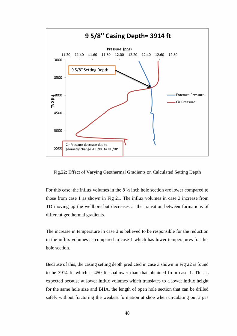
4.4.3 Case 3: Effect of Variations in formations geothermal gradients ....... 47

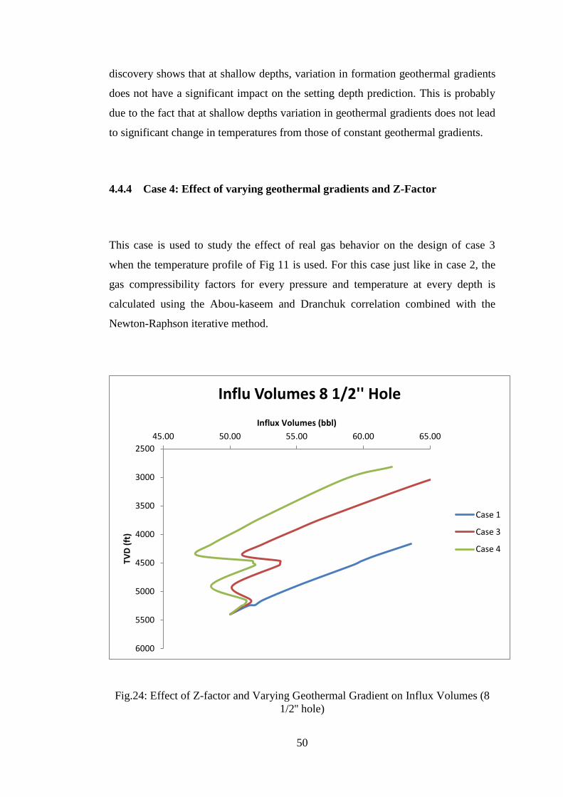
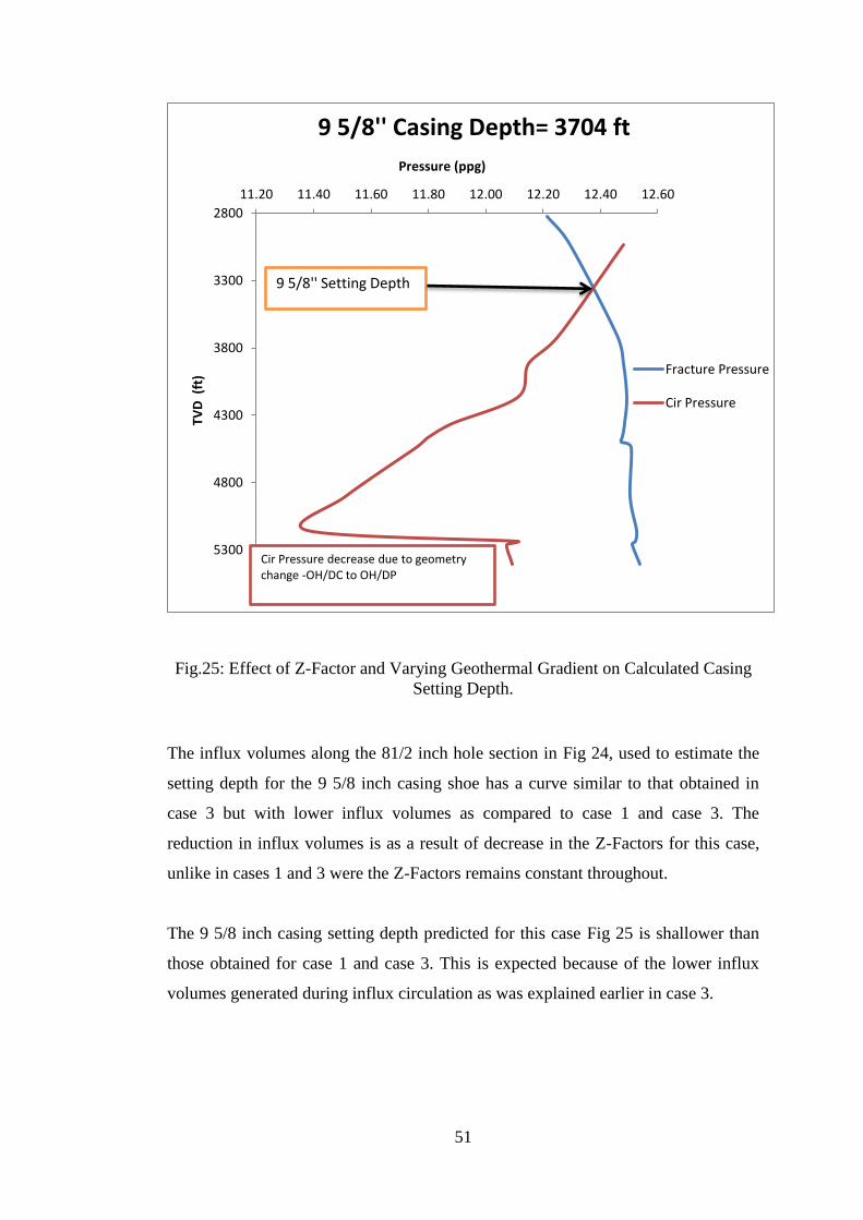
4.4.4 Case 4: Effect of varying geothermal gradients and Z-Factor ............ 50

CHAPTER 5 .............................................................................................................. 54

CONCLUSIONS AND RECOMMENDATIONS ................................................ 54

5.1 Conclusions ................................................................................................. 54

5.2 Recommendations ....................................................................................... 55

REFERENCES .......................................................................................................... 56

APPENDICES ........................................................................................................... 58

viii

LIST OF FIGURES

Fig.1: Kick tolerance at initial shut-in conditions and with mud weight increased [2]

..................................................................................................................................... 8

Fig.2: Kick tolerance with influx at shoe [2] ............................................................... 8

Fig.3: Choosing casing setting depths with and without kick tolerance [2] ................ 9

Fig.4: Proposed well Architectures [6] ...................................................................... 12

Fig.5: Pressure/Temperature phase diagram for pure gases [19] .............................. 20

Fig.6: Pressure/Temperature phase diagram for mixtures [16] ................................. 21

Fig.7: Compressibility factors for natural gas (Standing and Kartz chart) [16] ........ 25

Fig.8: Flow Chart ....................................................................................................... 28

Fig.9: Well Trajectory ............................................................................................... 34

Fig.10: Nearly Constant Temperature Gradient Profile ............................................ 38

Fig.11: Varying Temperature Gradients Profile ........................................................ 38

Fig.12: Influx Volumes along 8 ½ '' Hole (Case 1) ................................................... 39

Fig.13: Casing Setting Depth Calculated Using Kick Tolerance (Case 1) ................ 40

Fig.14: Influx Volumes along 12 1/4'' Hole (Case 1) ................................................ 41

Fig.15: Casing Setting Depth Calculated Using Kick Tolerance (Case 1) ................ 41

Fig.16: Effect of Z-Factor on influx Volumes along 8 1/2'' Hole ............................. 43

Fig.17: Effect of Z-Factor on Calculated Casing Setting Depth ............................... 43

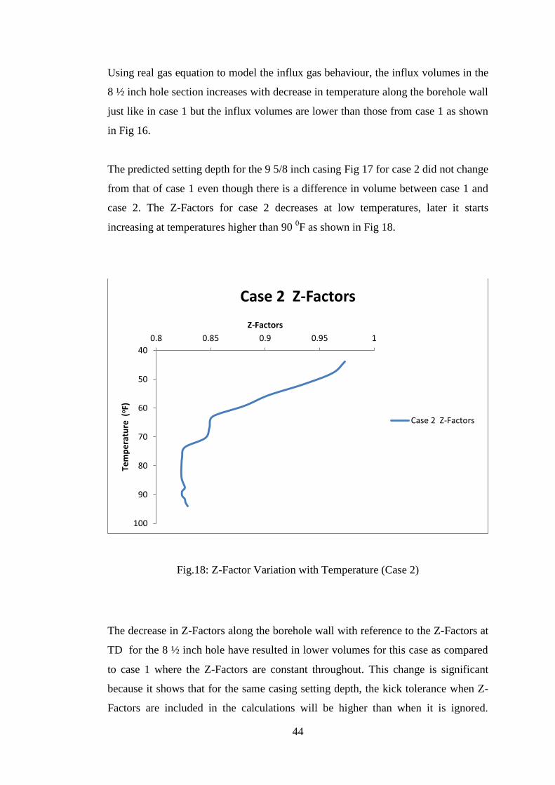
Fig.18: Z-Factor Variation with Temperature (Case 2) ............................................. 44

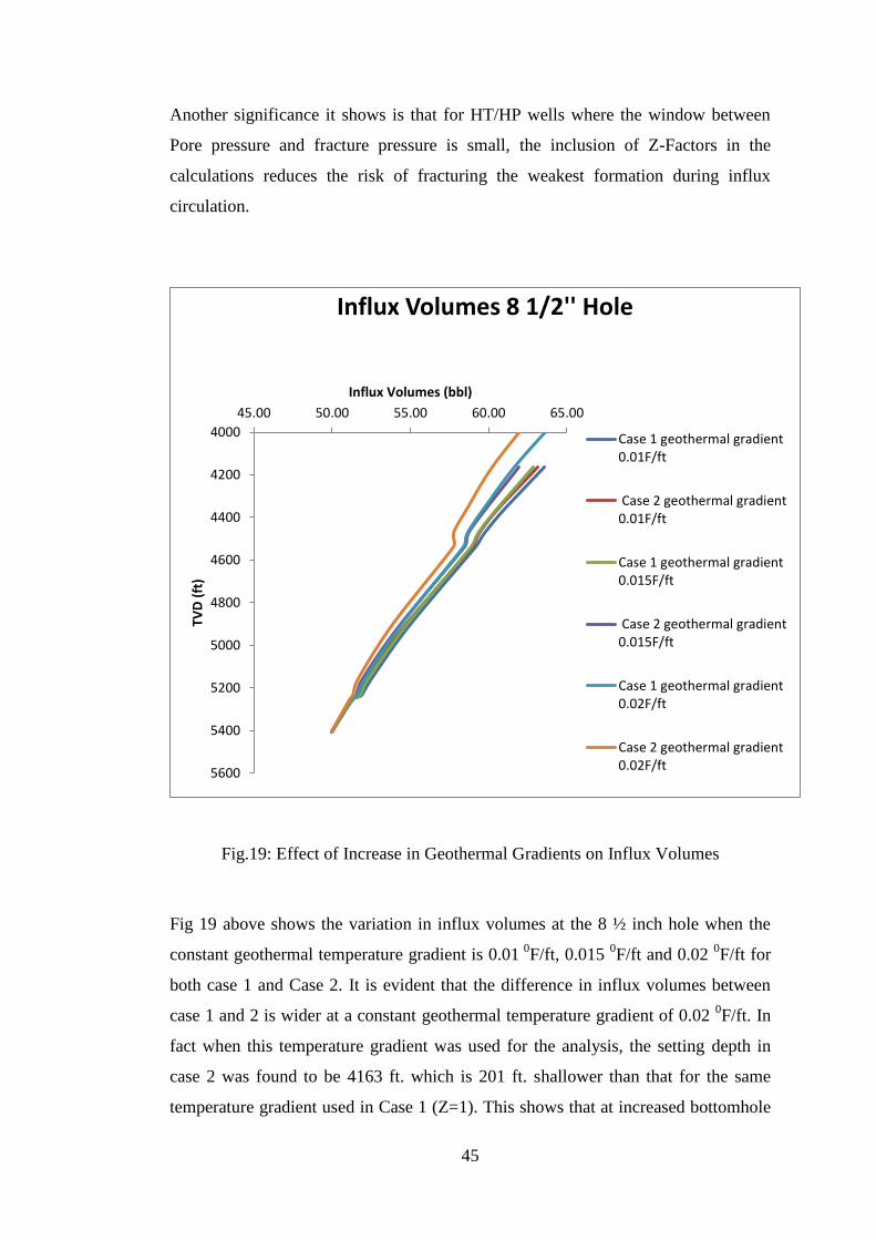
Fig.19: Effect of Increase in Geothermal Gradients on Influx Volumes .................. 45

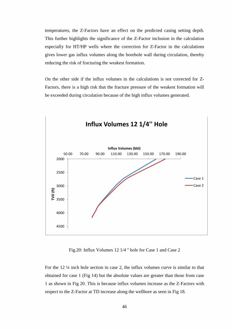
Fig.20: Influx Volumes 12 1/4 '' hole for Case 1 and Case 2 .................................... 46

Fig.21: Effect of varying Geothermal Gradients on Influx Volumes (8 ½’’ Hole) ... 47

Fig.22: Effect of Varying Geothermal Gradients on Calculated Setting Depth ........ 48

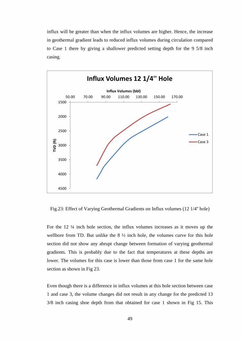
Fig.23: Effect of Varying Geothermal Gradients on Influx volumes (12 1/4'' hole) . 49

Fig.24: Effect of Z-factor and Varying Geothermal Gradient on Influx Volumes (8

1/2'' hole) ................................................................................................................... 50

Fig.25: Effect of Z-Factor and Varying Geothermal Gradient on Calculated Casing

Setting Depth. ............................................................................................................ 51

Fig.26: Effect of Z-Factor and Varying Geothermal Gradients on Influx Volumes

(12 1/4'' hole) ............................................................................................................. 52

Fig.27: Z-Factor Variation with Temperature for Case 4 .......................................... 53

ix

Fig.28: Pore Pressure and Fracture Pressure Profiles ................................................ 58

Fig.29: Z-Factors against TVD .................................................................................. 58

Fig.30: Z-Factors against Depth ................................................................................ 59

x

LIST OF TABLES

Table 1: Well Parameters for Simulation .................................................................. 33

Table 2: Pore and Fracture Pressure Data ................................................................. 35

xi

ABBREVIATIONS

TVD = True Vertical Depth

TD = Total Depth

OH = Open Hole

DC = Drill Collar

DP = Drill Pipe

BHA = Bottom Hole Assembly.

ppg = Pounds per gallon

Fig = Figure

Cir = Circulating

xii

NOMENCLATURES

Wn= New mud weight (ppg)

Wex= Existing mud weight (ppg)

Pcmax= Maximum allowable shu-in casing pressure (psi)

Dh= True vertical depth of hole (ft)

= Kick tolerance including effect of influx (lbm/gal)

= Maximum allowable shut-in casing pressure (psi)

= Gradient of influx (psi/ft)

= Length of influx (ft)

= True vertical depth of hole (ft)

D = Final well depth (ft)

Dcs = Casing shoe setting depth (ft)

= Fracture equivalent density (ppg)

= Mud density (ppg)

Hk = Height of kick calculated (ft)

= Kick density (ppg)

= Equivalent circulating density at casing shoe setting depth (ppg)

= Normalised gas velocity

= Fluid distribution coefficient

= Homogenous Velocity (m/s)

= Slip velocity (m/s)

P= Pressure

V= Volume

T= Temperature

n= number of moles (mass divided by molecular weight)

Rg = Universal gas constant.

Tc = Critical Temperature

Pc = Critical Pressure

= Pressure at the bottom hole (psi)

= Pore pressure at TD (ppg)

= TVD of well (ft)

= Mud weight (psi/ft)

xiii

= Height of kick (ft)

= Casing shoe depth (ft)

= Hydrostatic pressure of influx (psi)

= Influx gas gravi

= Temperature (0R)

= Gas compressibility (Z) Factor

= Influx Volume (bbl)

= Annulus Capacity factor (bbl/ft)

= Initial influx volume at TD (bbl)

= Pressure (psi), Temperature and Z-Factor at the bottom hole

= Pressure (psi), Temperature and Z-Factors at the depths

1

CHAPTER 1

INTRODUCTION

1.1 Background

The appropriate selection of casing setting depths for a well is one of the most

important aspects of a well design. It is essential for various reasons. Among these

reason includes for isolating troublesome hole sections, reducing torque and drag,

completion purposes, regulatory requirements and well control considerations.

Casing setting depths are traditionally selected based on mud weights. In this

method, the pore pressures, fracture pressure and mud weights are used together to

select casing setting points. The mud weights are derived by adding an appropriate

overbalance to the pore pressure to maintain primary well control but they are also

maintained below the fracture gradient to prevent fracturing the formation. In

essence, casing seats are selected so that the minimum mud density does not exceed

the allowable maximum density. The application of this method relies greatly on

accurate estimations of pore and fracture pressures. Selecting casing seat based on

mud weights will not provide sufficient fracture integrity to control a gas kick,

meaning there is a danger that the pressure generated during the process of

circulating the kick out of well will exceed the fracture gradient of the weakest

formation in the open hole presumable the formation at casing shoe or at any other

critical depth leading to loss of well control and possibly an underground blowout.

Hence, the current industry practice of selecting casing setting depths has included

well control consideration through the kick tolerance concept.

Kick tolerance is a fundamental concept in well design. Its applications on well

design for casing setting depth selection purposes have made drilling much more

safe and economical. It defines the number of casing in a well and also indicates

whether it is safe to continue drilling or a new casing string should be run in order to

2

reach the target depth. In as much as the concept is fundamental in well design it has

been defined in various ways by different operators. Some of the definitions used are

highlighted below[1]:

-The largest volume of influx that can be removed from the well safely based on the

results of either a Leak off test (LOT) or formation integrity test (FIT or limit

test).[1]

•The capability of the wellbore to withstand a state of pressure generated during well

control operations without fracturing the weakest formation.[1]

•The maximum increase in mud weight allowed by the pressure integrity test (LOT

or FIT) of the casing shoe with no influx in the wellbore.[1]

•The maximum allowable pore pressure, expressed in equivalent mud density such

that if a kick with specified volume occurs at a particular depth with a specific

drilling fluid the well could be closed down and the kick circulated out safely

without fracturing the weakest section in the open hole. [1]

•Maximum influx to equal the Maximum Allowable Annular Surface Pressure

(MAASP).[1]

•The maximum kick volume that can be taken into the wellbore and circulated out

without fracturing the formation at the weakest point (commonly the casing shoe),

given the difference between pore pressure and mud weight in use ( kick intensity).

•The maximum volume of a swabbed kick that can be circulated out without

fracturing the previous casing shoe

•An estimate of the volume of gas influx at bottomhole condition that can be safely

shut in and circulated out of the well.

•The maximum kick intensity that a well can tolerate before lost circulation is

experienced at the last casing seat.

3

The conventional approach of selecting casing setting depth based on kick tolerance

assumes a bubble of gas influx into the wellbore and uses it to calculate the pressure

generated inside the wellbore when the gas is circulated out of the well assuming

constant geothermal gradient and ideal gas behavior. The ideal gas law is thus used

to calculate the volumes at various depths in the well. The influx height can then be

calculated using the annular capacity factor. The driller’s method (worst case

scenario) of kick circulation is then employed to compute the internal pressure

generated during the kick circulation process. These pressures are then compared to

the fracture gradients at different depths to determine the casing seat depth. The

internal pressure prediction is done on a look forward basis as drilling proceeds into

area of changing pore pressure regimes. The Driller’s method equation of

calculating the internal kick circulation pressures depends on the pore at next TD,

the mud weight, the geometry of well and the nature of influx fluid.

The method that assumes gas influx enters as slug into the well and remains as slug

during circulation is a simple model that leads to a conservative solution as

compared to those obtained by using a gas kick simulator. For this reason Gas kick

simulators were developed in order to accurately represent what happens in the

wellbore during kick circulation so that accurate internal pressures would be

calculated thereby minimizing the risk of fracturing the formations at the casing

shoe or any other critical depth.

1.2 Problem Statement

The current industry practice of estimating casing setting depths using kick tolerance

assumes a constant geothermal gradient and uses ideal gas law to model the gas as it

moves up the wellbore. The issues with this approach is that, the geothermal

gradient might not be constant from one formation to another and also in order to

model accurately what happens in a well during well control procedures requires

that the deviation from ideal behavior (real gas behavior) be considered. Neglecting

the effects of such variations will have a significant impact on whether a casing

should be set shallower or deeper in a well.

4

As wells are now drilled in more challenging environments such as HT/HP wells in

which there is a small window between pore and fracture pressure, variations on

how kick tolerance is calculated can lead to dangerous drilling environment and can

also lead to expensive well design.

1.3 Objectives

The main objectives of this project are:

a) To understand gas behavior in terms of PVT relationship as it is circulated

out of a well during well control procedures.

b) To develop a procedure for casing setting depth design that takes into

account the effect of geothermal temperature changes and real gas behavior

and study how these effects affect the selection of casing setting depths

1.4 Scope of Study

The purpose of the project is to study what effects gas compressibility factors and

subsurface geothermal temperature variations has on calculation of casing seats

using kick tolerance concept. A model that is based on a single gas bubble of an

influx will be built on excel macro. The model will be used to study the how the

influx volume will change as it moves up the well bore as a real gas in a varying

formation geothermal gradient and then highlight the differences when a model of

ideal gas behavior and constant geothermal gradient is applied instead. The model

will then be used to calculate casing seats using real gas law and changing

subsurface formation geothermal gradients and compare the results obtained from

the ideal gas behavior and constant geothermal gradients model, in order to quantify

the effects the compressibility factors and varying geothermal gradients has on the

design.

5

CHAPTER 2

LITERATURE REVIEW AND THEORY

Kick tolerance has been a controversial subject defined in different ways by

different operators. This controversy has led to the publication of lots of technical

papers to address the subject. This chapter summarises the pertinent literature found

on kick tolerance. It contains an overview of the kick tolerance concept, a review on

gas kick simulation models to model and predict gas kick volumes and bottomhole

pressure behavior. An overview on the use of equations of state to calculate

compressibility (Z-factors) will also be presented.

2.1 The Kick Tolerance Concept

Kick tolerance defined as the maximum difference between the pore pressure and

existing mud weight that can be allowed for safe circulation of the influx during well

control without fracturing the weakest formation in the open hole is a fundamental

concept in well design. It specifies the number of casing strings to be used in a well

as well as indicating whether it is safe to continue drilling or to run a casing. The use

of kick tolerance in well design and operational well control to avoid kicks or lost

circulation and blow outs is been critical to the successful drilling of wells. In light

of its significance in well design and drilling, lots of literature has been published on

this topic to make it more understandable and reduce the controversies surrounding

it.

Early works by K.P Redmann [2], Otto Santos [3] , Antonio Carlos et al [4]were

concerned about highlighting the significance of kick tolerance in well design and

how it can be used to determine casing setting depths. Adetola, Isaac and Olayinka

[5] proposed a stochastic model for selecting the appropriate kick tolerance for a

given region. Further works by Oumer, Taufiqurranchman, Perrucho and Yunnus [6]

dealt with the use of kick tolerance to design wells in a shallow gas field.

6

Helio Santos, Catak and Sandeep[1] highlighted the Misconceptions associated with

the kick tolarnce concept and the consequences they bring to well design.

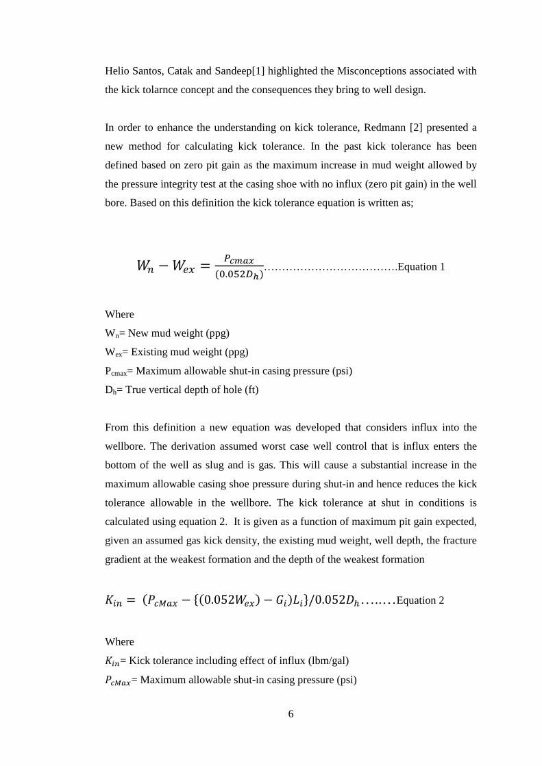
In order to enhance the understanding on kick tolerance, Redmann [2] presented a

new method for calculating kick tolerance. In the past kick tolerance has been

defined based on zero pit gain as the maximum increase in mud weight allowed by

the pressure integrity test at the casing shoe with no influx (zero pit gain) in the well

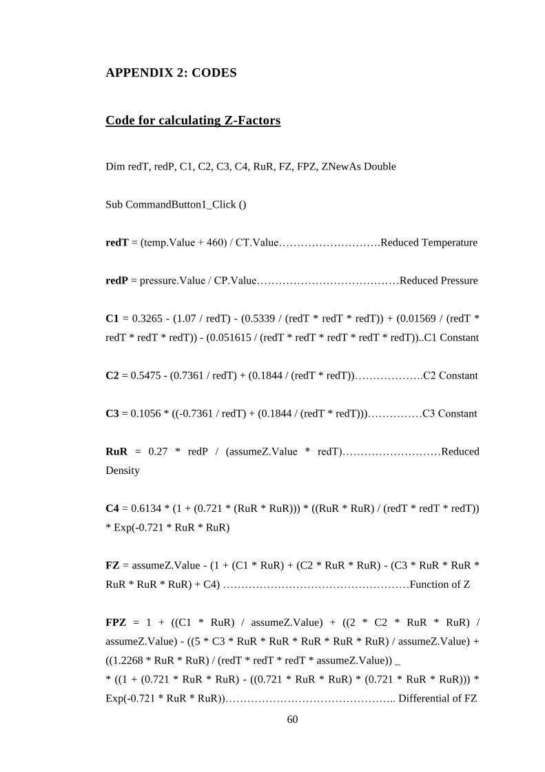
bore. Based on this definition the kick tolerance equation is written as;

……………………………….Equation 1

Where

Wn= New mud weight (ppg)

Wex= Existing mud weight (ppg)

Pcmax= Maximum allowable shut-in casing pressure (psi)

Dh= True vertical depth of hole (ft)

From this definition a new equation was developed that considers influx into the

wellbore. The derivation assumed worst case well control that is influx enters the

bottom of the well as slug and is gas. This will cause a substantial increase in the

maximum allowable casing shoe pressure during shut-in and hence reduces the kick

tolerance allowable in the wellbore. The kick tolerance at shut in conditions is

calculated using equation 2. It is given as a function of maximum pit gain expected,

given an assumed gas kick density, the existing mud weight, well depth, the fracture

gradient at the weakest formation and the depth of the weakest formation

{ } …..…Equation 2

Where

= Kick tolerance including effect of influx (lbm/gal)

= Maximum allowable shut-in casing pressure (psi)

7

= Existing or current mud weight (lbm/gal)

= Gradient of influx (psi/ft)

= Length of influx (ft)

= True vertical depth of hole (ft)

The pressure of the influx when it is circulated to the casing shoe is calculated using

the driller’s method of well control. Maximum shoe pressure will occur at the shoe

when the top of the influx has been circulated to the casing shoe. The pressure

generated at the weakest formation presumable the casing shoe is calculated in an

iterative manner using the pressure/volume equation to predict both the pressure and

volume of the shut-in influx as it is circulated to the casing shoe. The equivalent

mud weight Weq, at the shoe may then be determined and a new kick tolerance value

computed from:

……….............Equation 3

Where,

= Circulation Kick Tolerance

= Shoe test (ppg)

= Equivalent mud weight (psi)

The value of kick tolerance computed from equation (2) is compared to that from

equation (3), the lesser of the two values is used as the kick tolerance.

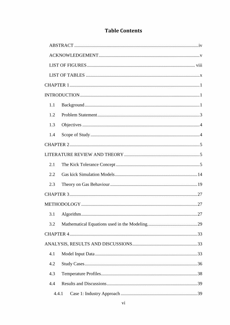
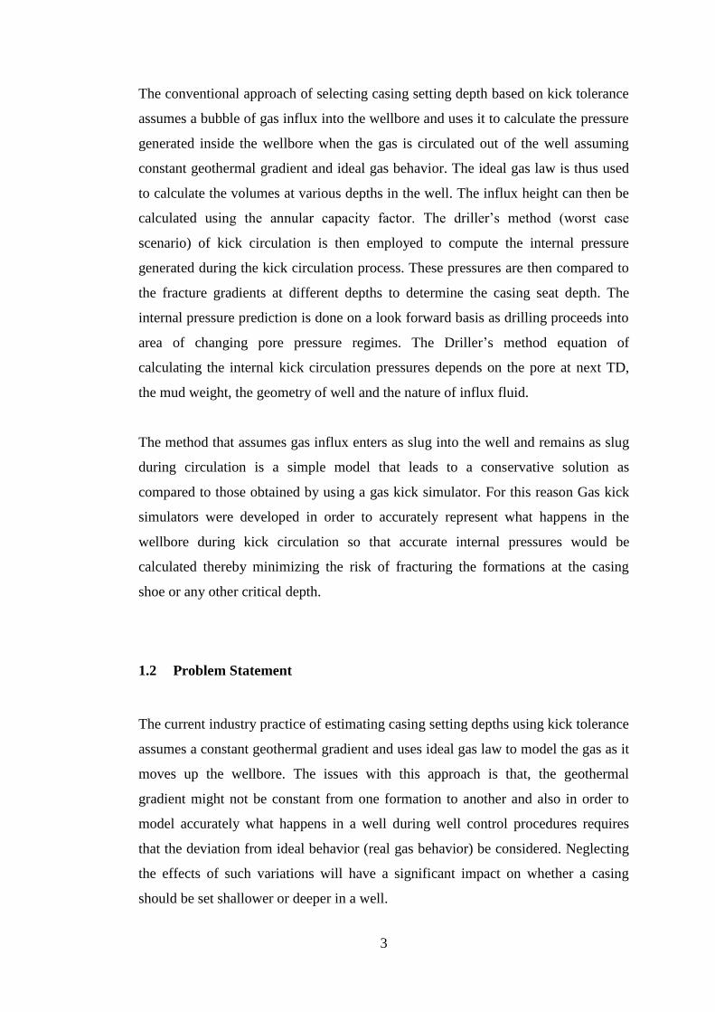
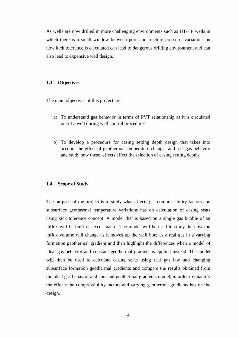
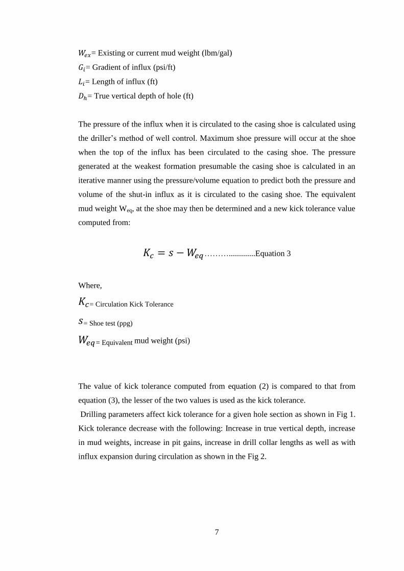
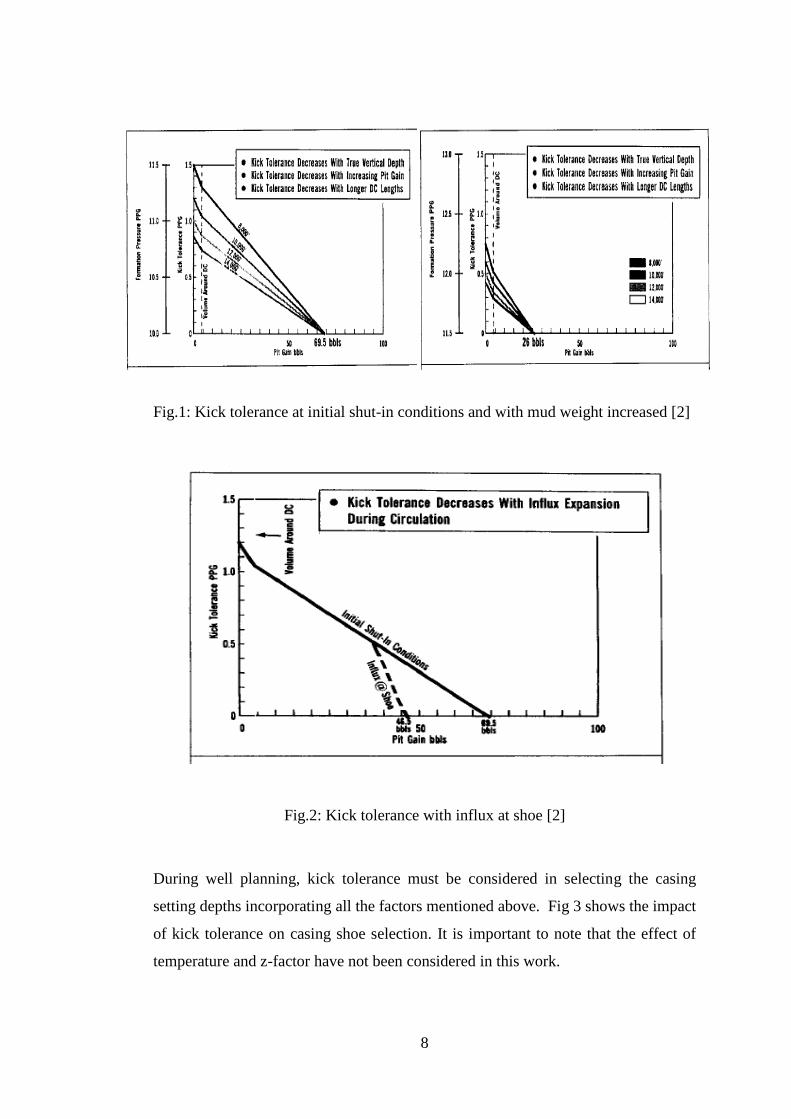
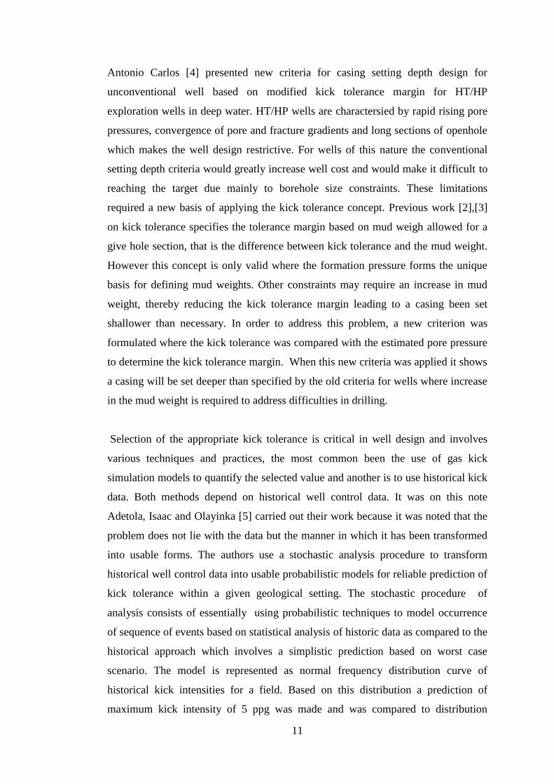
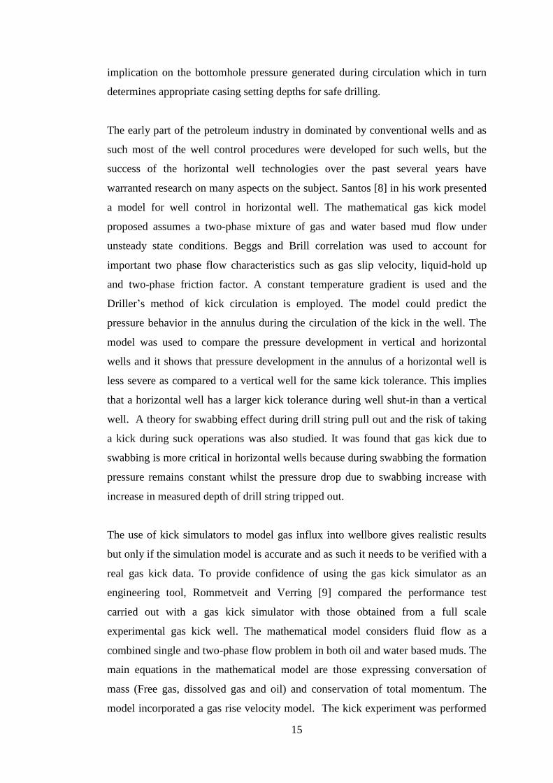
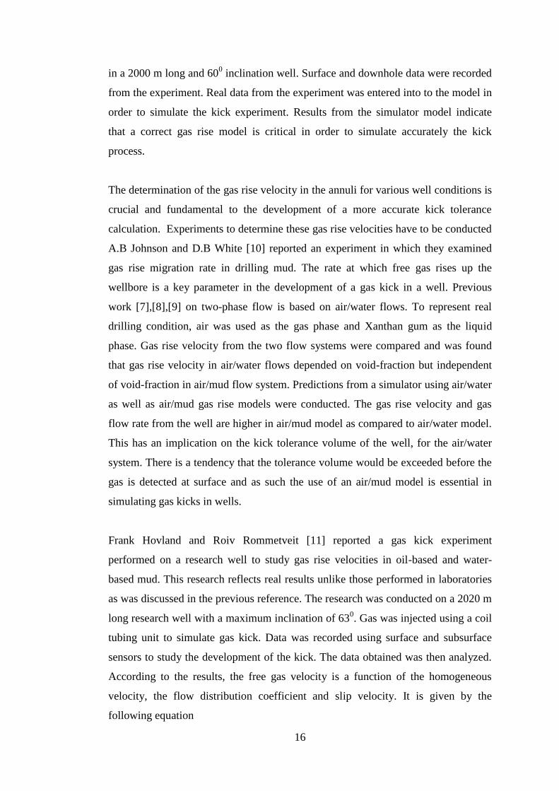
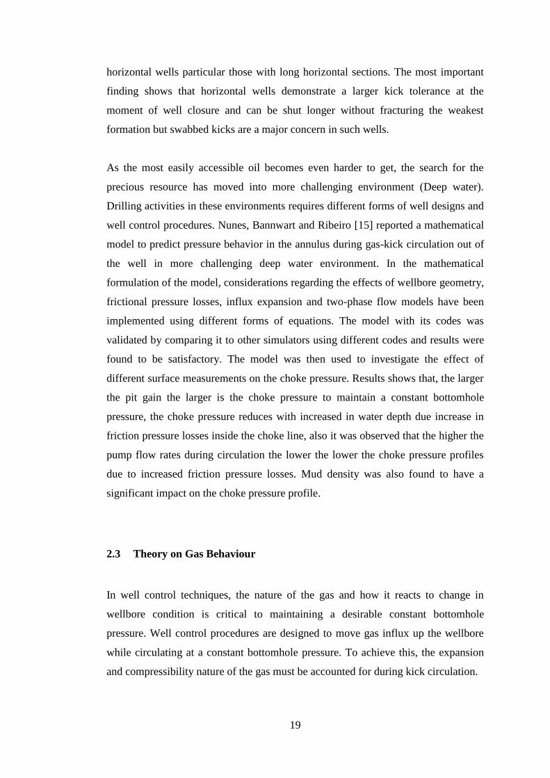
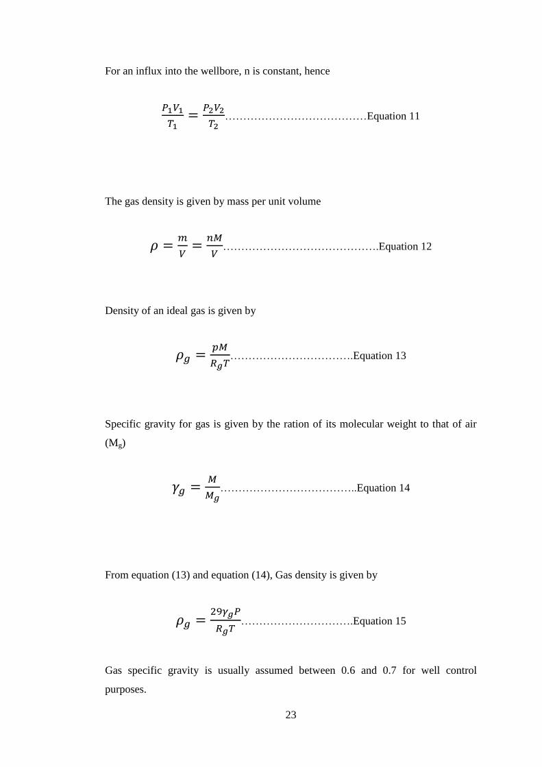
Drilling parameters affect kick tolerance for a given hole section as shown in Fig 1.

Kick tolerance decrease with the following: Increase in true vertical depth, increase

in mud weights, increase in pit gains, increase in drill collar lengths as well as with

influx expansion during circulation as shown in the Fig 2.

8

Fig.1: Kick tolerance at initial shut-in conditions and with mud weight increased [2]

Fig.2: Kick tolerance with influx at shoe [2]

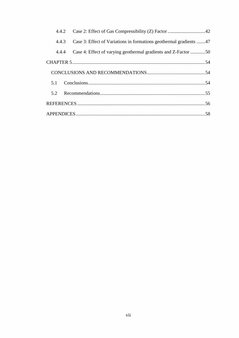
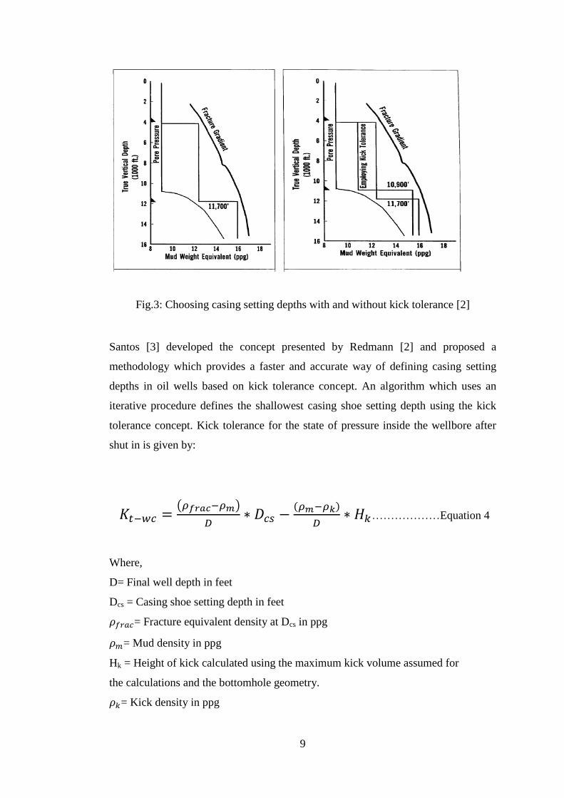
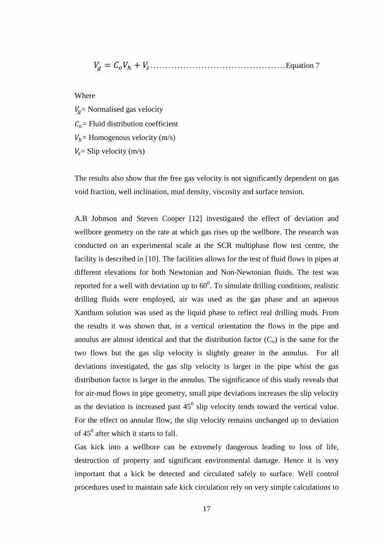
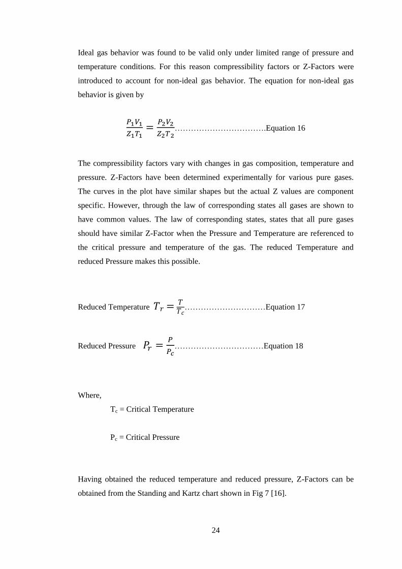
During well planning, kick tolerance must be considered in selecting the casing

setting depths incorporating all the factors mentioned above. Fig 3 shows the impact

of kick tolerance on casing shoe selection. It is important to note that the effect of

temperature and z-factor have not been considered in this work.

9

Fig.3: Choosing casing setting depths with and without kick tolerance [2]

Santos [3] developed the concept presented by Redmann [2] and proposed a

methodology which provides a faster and accurate way of defining casing setting

depths in oil wells based on kick tolerance concept. An algorithm which uses an

iterative procedure defines the shallowest casing shoe setting depth using the kick

tolerance concept. Kick tolerance for the state of pressure inside the wellbore after

shut in is given by:

( )

………………Equation 4

Where,

D= Final well depth in feet

Dcs = Casing shoe setting depth in feet

= Fracture equivalent density at Dcs in ppg

= Mud density in ppg

Hk = Height of kick calculated using the maximum kick volume assumed for

the calculations and the bottomhole geometry.

= Kick density in ppg

10

The casing shoe setting depth should satisfy the following design criteria

≤

Replacing in equation (4) by the maximum pressure generated at the shoe and

using a 0.5 ppg kick tolerance for well containment, equation (4) becomes

Equation 5

To determine the casing setting depth the fracture gradient of the formation is

compared to the pressure generated inside the wellbore during a well control

operation. The procedure involves guessing a casing setting depth, then calculating

the maximum pressure in the wellbore after shut-in, a kick tolerance of 0.5 ppg is

then added to this value, if the resulting value is equal to or less than the fracture

equivalent density then the guessed setting depth is the shallowest casing setting

depth. This procedure is continued until the optimum depth is obtained. The

procedure was applied to determine casing setting depth during kick circulation

using the driller’s method. For this situation, kick tolerance is given by the equation:

………………………………….Equation 6

Where

= Equivalent circulating density at casing shoe setting depth in ppg

In this method, the pressure generated inside the wellbore at every depth is predicted

and compared to the fracture pressure at the same depth. The procedure is similar to

the one used for well containment. The model showed that the higher the kick

tolerance volume the greater the shallowest casing setting depth.

11

Antonio Carlos [4] presented new criteria for casing setting depth design for

unconventional well based on modified kick tolerance margin for HT/HP

exploration wells in deep water. HT/HP wells are charactersied by rapid rising pore

pressures, convergence of pore and fracture gradients and long sections of openhole

which makes the well design restrictive. For wells of this nature the conventional

setting depth criteria would greatly increase well cost and would make it difficult to

reaching the target due mainly to borehole size constraints. These limitations

required a new basis of applying the kick tolerance concept. Previous work [2],[3]

on kick tolerance specifies the tolerance margin based on mud weigh allowed for a

give hole section, that is the difference between kick tolerance and the mud weight.

However this concept is only valid where the formation pressure forms the unique

basis for defining mud weights. Other constraints may require an increase in mud

weight, thereby reducing the kick tolerance margin leading to a casing been set

shallower than necessary. In order to address this problem, a new criterion was

formulated where the kick tolerance was compared with the estimated pore pressure

to determine the kick tolerance margin. When this new criteria was applied it shows

a casing will be set deeper than specified by the old criteria for wells where increase

in the mud weight is required to address difficulties in drilling.

Selection of the appropriate kick tolerance is critical in well design and involves

various techniques and practices, the most common been the use of gas kick

simulation models to quantify the selected value and another is to use historical kick

data. Both methods depend on historical well control data. It was on this note

Adetola, Isaac and Olayinka [5] carried out their work because it was noted that the

problem does not lie with the data but the manner in which it has been transformed

into usable forms. The authors use a stochastic analysis procedure to transform

historical well control data into usable probabilistic models for reliable prediction of

kick tolerance within a given geological setting. The stochastic procedure of

analysis consists of essentially using probabilistic techniques to model occurrence

of sequence of events based on statistical analysis of historic data as compared to the

historical approach which involves a simplistic prediction based on worst case

scenario. The model is represented as normal frequency distribution curve of

historical kick intensities for a field. Based on this distribution a prediction of

maximum kick intensity of 5 ppg was made and was compared to distribution

12

generated using results from a gas kick simulation model which incorporates data

from the same field. The results from both predictions were consistent thus

validating the model. The historical and the stochastic approaches were applied to

determine kick tolerance for the drilling of the 8 ½’’ hole section of a horizontal

well, it was found that the stochastic approach gave a lower volume allowing the

well to drilled to the target depth as compared to the historical approach which gave

a higher volumes thus requiring an extra casing string to reach the target depth and

as such increasing the well cost. The stochastic approach provides a more realistic

method for selecting appropriate kick tolerance to be used in the design of wells.

However the stochastic approach is only valid for regions whose data have been

used to generate it.

In equation (5) the height of the gas in the open hole is calculated by dividing the

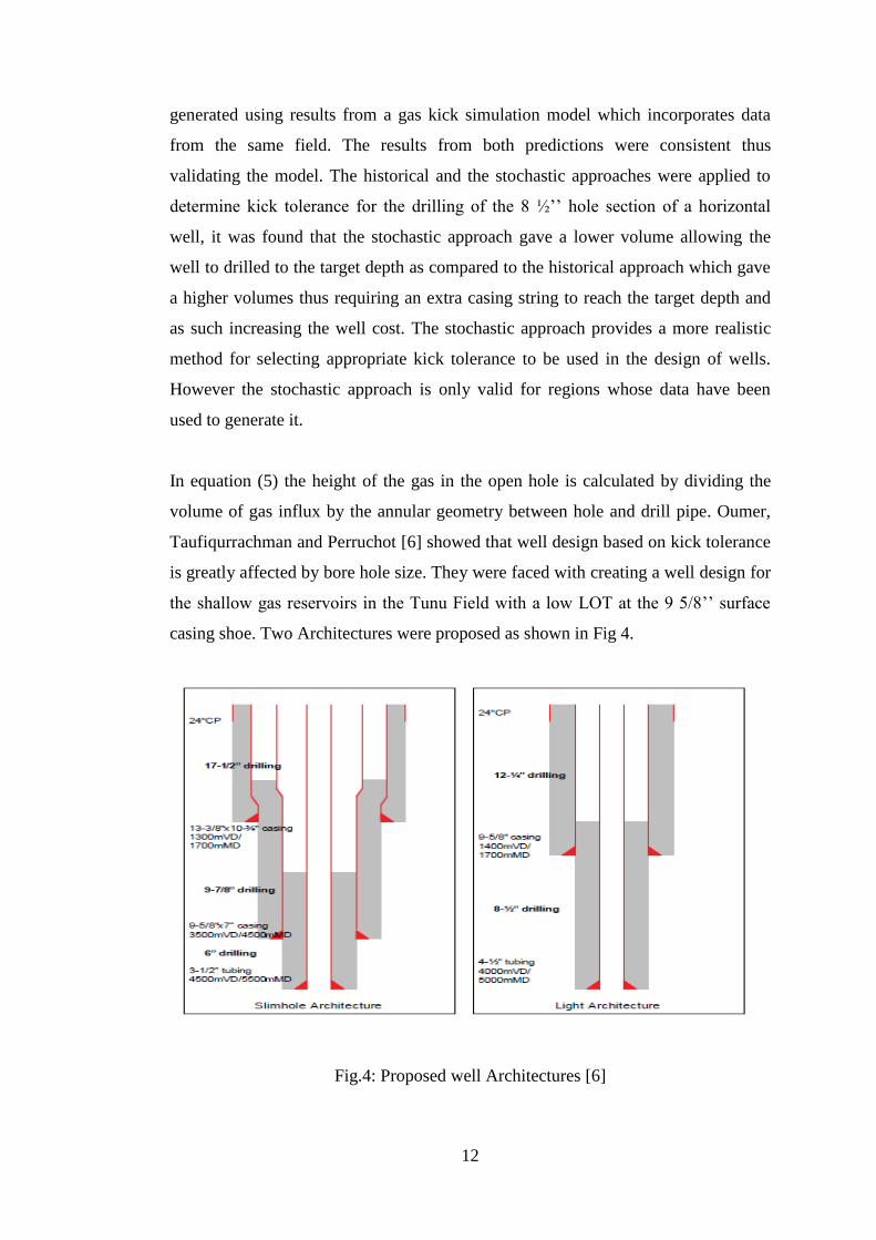
volume of gas influx by the annular geometry between hole and drill pipe. Oumer,

Taufiqurrachman and Perruchot [6] showed that well design based on kick tolerance

is greatly affected by bore hole size. They were faced with creating a well design for

the shallow gas reservoirs in the Tunu Field with a low LOT at the 9 5/8’’ surface

casing shoe. Two Architectures were proposed as shown in Fig 4.

Fig.4: Proposed well Architectures [6]

13

Both designs were investigated for casing setting depth that can permit the

circulation of 5 m3 of influx gas. From the results it was found that the first

architecture gave satisfactory results for all depths investigated but the second

architecture gave limitations in setting depths with regards to kick tolerance, hence

showing that the reduction on the hole size in the second architecture have impacted

on the design. It is important to note that when the kick tolerance was reduced to 3

m3 the second architecture gave satisfactory results in terms of maximum TD

drilled.

The concept of kick tolerance have been defined and applied in different ways by

different operators in well design and drilling implementation as was mentioned

earlier in the background. Santos, Catak and Sandeep [1] carried out a review of the

fundamental concepts in the application of kick tolerance and they found that few

misconceptions that have been made in applying the kick tolerance concept. They

also studied the consequences they bring to well design. Amongst the

misconceptions is the assumption that an approach utilizing a single bubble model

ignoring the effect of temperature and gas compressibility factor in the final

calculations will always result in a conservative solution. The current approach for

calculating kick tolerance for a given hole section does not take into account the

effect changes in temperature along the wellbore. In this study the effect of

temperature changes on the influx volume was taken into account by using Charles

Law. The results show that the effect of temperature resulted in a higher kick

tolerance volumes as compared to the current approach which assumes constant

temperature in the well bore. The effect of compressibility factor was also

investigated. The Z-factor is used to allow for using the ideal gas law to model the

behavior of real gases. Compressibility factor were for conditions along the

openhole and the results shows that the smaller the Z-factor the higher the kick

tolerance. It must be stressed here that the temperature been used is that of the

constant geothermal gradient, in this project the effect of varying temperature

gradients across different formation types in the kick tolerance calculations will be

studied coupled with changes in the compressibility factors for the stated

temperatures and pressures in the formations.

14

2.2 Gas kick Simulation Models

The previous discussions on the use of the kick tolerance concept in well design

assume the influx as slug and remains as slug during circulation. This method gives

a conservative solution to the kick tolerance calculations. The flow of gas influx in

the wellbore is a complex process which involves the interaction of internal sub-

processes as well as external factors such as well geometry, mud and gas properties,

reservoir conditions etc. that defines the character of the kick. In order to accurately

describe this flow process in the wellbore, gas kick simulators are needed. A lot of

work has been done on this subject that has resulted in the publication of many

technical papers.

D.B White and Walton [7] developed a computer gas kick model for kicks in water

and oil based mud. The model is based on the full mass (mud and gas) and

momentum (gas-mud mixture) equations. The mathematical representation of the

model took into account wellbore hydrodynamics by modeling the distribution of

drilling mud, dissolved gas and free gas at different times and different positions, it

also accounted for flow of gas from the formation by deriving an equation from the

combination of the equation of conservation of mass, an equation of state of the

fluid and Darcy’s law for flow in porous medium. Equations accounting for Gas

dissolution, variation of rheological parameters of the mud with pressure and

temperature (Casson Model), frictional pressure losses, dispersion of dissolved gas

and an empirical correlation for gas rise in the drilling mud were used. The model

also considered well plan geometry and took into account the variation of downhole

temperatures during circulation. The model was validated with experimental data for

both oil-based and water-based mud. When a simulation was run using criteria of

10bbl pit gain, gas kick detections in oil-based mud took longer to detect as

compared to water based mud. During the kill process in the two cases (water and

oil based muds) there is an earlier arrival of gas in the water based mud test as

transport is dominated by the rise of free gas. In the oil based mud, the initial pit

gain is at a lower rate as the gas expansion is less significant. This has an

15

implication on the bottomhole pressure generated during circulation which in turn

determines appropriate casing setting depths for safe drilling.

The early part of the petroleum industry in dominated by conventional wells and as

such most of the well control procedures were developed for such wells, but the

success of the horizontal well technologies over the past several years have

warranted research on many aspects on the subject. Santos [8] in his work presented

a model for well control in horizontal well. The mathematical gas kick model

proposed assumes a two-phase mixture of gas and water based mud flow under

unsteady state conditions. Beggs and Brill correlation was used to account for

important two phase flow characteristics such as gas slip velocity, liquid-hold up

and two-phase friction factor. A constant temperature gradient is used and the

Driller’s method of kick circulation is employed. The model could predict the

pressure behavior in the annulus during the circulation of the kick in the well. The

model was used to compare the pressure development in vertical and horizontal

wells and it shows that pressure development in the annulus of a horizontal well is

less severe as compared to a vertical well for the same kick tolerance. This implies

that a horizontal well has a larger kick tolerance during well shut-in than a vertical

well. A theory for swabbing effect during drill string pull out and the risk of taking

a kick during suck operations was also studied. It was found that gas kick due to

swabbing is more critical in horizontal wells because during swabbing the formation

pressure remains constant whilst the pressure drop due to swabbing increase with

increase in measured depth of drill string tripped out.

The use of kick simulators to model gas influx into wellbore gives realistic results

but only if the simulation model is accurate and as such it needs to be verified with a

real gas kick data. To provide confidence of using the gas kick simulator as an

engineering tool, Rommetveit and Verring [9] compared the performance test

carried out with a gas kick simulator with those obtained from a full scale

experimental gas kick well. The mathematical model considers fluid flow as a

combined single and two-phase flow problem in both oil and water based muds. The

main equations in the mathematical model are those expressing conversation of

mass (Free gas, dissolved gas and oil) and conservation of total momentum. The

model incorporated a gas rise velocity model. The kick experiment was performed

16

in a 2000 m long and 600 inclination well. Surface and downhole data were recorded

from the experiment. Real data from the experiment was entered into to the model in

order to simulate the kick experiment. Results from the simulator model indicate

that a correct gas rise model is critical in order to simulate accurately the kick

process.

The determination of the gas rise velocity in the annuli for various well conditions is

crucial and fundamental to the development of a more accurate kick tolerance

calculation. Experiments to determine these gas rise velocities have to be conducted

A.B Johnson and D.B White [10] reported an experiment in which they examined

gas rise migration rate in drilling mud. The rate at which free gas rises up the

wellbore is a key parameter in the development of a gas kick in a well. Previous

work [7],[8],[9] on two-phase flow is based on air/water flows. To represent real

drilling condition, air was used as the gas phase and Xanthan gum as the liquid

phase. Gas rise velocity from the two flow systems were compared and was found

that gas rise velocity in air/water flows depended on void-fraction but independent

of void-fraction in air/mud flow system. Predictions from a simulator using air/water

as well as air/mud gas rise models were conducted. The gas rise velocity and gas

flow rate from the well are higher in air/mud model as compared to air/water model.

This has an implication on the kick tolerance volume of the well, for the air/water

system. There is a tendency that the tolerance volume would be exceeded before the

gas is detected at surface and as such the use of an air/mud model is essential in

simulating gas kicks in wells.

Frank Hovland and Roiv Rommetveit [11] reported a gas kick experiment

performed on a research well to study gas rise velocities in oil-based and water-

based mud. This research reflects real results unlike those performed in laboratories

as was discussed in the previous reference. The research was conducted on a 2020 m

long research well with a maximum inclination of 630. Gas was injected using a coil

tubing unit to simulate gas kick. Data was recorded using surface and subsurface

sensors to study the development of the kick. The data obtained was then analyzed.

According to the results, the free gas velocity is a function of the homogeneous

velocity, the flow distribution coefficient and slip velocity. It is given by the

following equation

17

………………………………………Equation 7

Where

= Normalised gas velocity

= Fluid distribution coefficient

= Homogenous velocity (m/s)

= Slip velocity (m/s)

The results also show that the free gas velocity is not significantly dependent on gas

void fraction, well inclination, mud density, viscosity and surface tension.

A.B Johnson and Steven Cooper [12] investigated the effect of deviation and

wellbore geometry on the rate at which gas rises up the wellbore. The research was

conducted on an experimental scale at the SCR multiphase flow test centre, the

facility is described in [10]. The facilities allows for the test of fluid flows in pipes at

different elevations for both Newtonian and Non-Newtonian fluids. The test was

reported for a well with deviation up to 600. To simulate drilling conditions, realistic

drilling fluids were employed, air was used as the gas phase and an aqueous

Xanthum solution was used as the liquid phase to reflect real drilling muds. From

the results it was shown that, in a vertical orientation the flows in the pipe and

annulus are almost identical and that the distribution factor (Co) is the same for the

two flows but the gas slip velocity is slightly greater in the annulus. For all

deviations investigated, the gas slip velocity is larger in the pipe whist the gas

distribution factor is larger in the annulus. The significance of this study reveals that

for air-mud flows in pipe geometry, small pipe deviations increases the slip velocity

as the deviation is increased past 450 slip velocity tends toward the vertical value.

For the effect on annular flow, the slip velocity remains unchanged up to deviation

of 450 after which it starts to fall.

Gas kick into a wellbore can be extremely dangerous leading to loss of life,

destruction of property and significant environmental damage. Hence it is very

important that a kick be detected and circulated safely to surface. Well control

procedures used to maintain safe kick circulation rely on very simple calculations to

18

calculate kick density, formation pressures and maximum casing shoe pressure from

hydrostatic calculations using surface measurements of pit gains, difference between

stabilized surface pressures in the drill string and the annulus, stabilized drill pipe

pressure and change in hydrostatic pressure as the influx moves up the well.

However, these calculations are subject to major errors. To address these errors,

Billingham, Thompson and White [13] reported a new method to analyse these

surface measurements and developed equations for pit gain and drill pipe pressures.

These equations were fitted to surface measurements to reveal important downhole

quantities. One such quantity is the maximum casing shoe pressure that would be

generated when circulating out a gas kick. Standard methods of predicting such

pressures assume gas exist as a single bubble and ideal gas behavior. These

calculations overestimated the true pressure. The gas influx was treated as a

distributed bubbly mixture of gas and mud which occupies a greater length of the

annulus. Down hole gas distribution was estimated using a rise cloud of influx gas in

drilling mud model instead of a function of void fraction. Gas was assumed to have

ideal gas behavior. These assumptions were incorporated into the model to improve

prediction of maximum casing shoe pressure and it gave a lower pressure than that

estimated using standard method. From the results it is seen that a good model of the

gas dynamics during kick enables the estimation of the distribution of the influx

which allows for a more accurate estimation of maximum casing shoe pressure as

compared to the single bubble approximation.

As was mentioned earlier, the successes of the application of the horizontal well

technologies for reservoir development have seen many research and investigation

conducted on the subject. Zhihua , Peden and Lemanczyk [14] performed simulation

studies on gas kick displacement in horizontal and conventional wells. The

simulation model was based on mass and pressure balance equations of mud and gas

as well as empirical correlations relating gas velocity to the average mixture plus the

relative slip velocity and equations of state for gas and mud. Their work is an

extension of previous works [7],[8],[10],[12],[13] done on the gas kick simulation.

The model was used to simulate kick in a horizontal well and vertical well to enable

comparison. The results show that the delta flow (flow-out minus flow-in at surface)

used for kick detection remains to be a sensitive parameter in horizontal wells, it

was also revealed that the effect of gas migration is considerably smaller in

19

horizontal wells particular those with long horizontal sections. The most important

finding shows that horizontal wells demonstrate a larger kick tolerance at the

moment of well closure and can be shut longer without fracturing the weakest

formation but swabbed kicks are a major concern in such wells.

As the most easily accessible oil becomes even harder to get, the search for the

precious resource has moved into more challenging environment (Deep water).

Drilling activities in these environments requires different forms of well designs and

well control procedures. Nunes, Bannwart and Ribeiro [15] reported a mathematical

model to predict pressure behavior in the annulus during gas-kick circulation out of

the well in more challenging deep water environment. In the mathematical

formulation of the model, considerations regarding the effects of wellbore geometry,

frictional pressure losses, influx expansion and two-phase flow models have been

implemented using different forms of equations. The model with its codes was

validated by comparing it to other simulators using different codes and results were

found to be satisfactory. The model was then used to investigate the effect of

different surface measurements on the choke pressure. Results shows that, the larger

the pit gain the larger is the choke pressure to maintain a constant bottomhole

pressure, the choke pressure reduces with increased in water depth due increase in

friction pressure losses inside the choke line, also it was observed that the higher the

pump flow rates during circulation the lower the lower the choke pressure profiles

due to increased friction pressure losses. Mud density was also found to have a

significant impact on the choke pressure profile.

2.3 Theory on Gas Behaviour

In well control techniques, the nature of the gas and how it reacts to change in

wellbore condition is critical to maintaining a desirable constant bottomhole

pressure. Well control procedures are designed to move gas influx up the wellbore

while circulating at a constant bottomhole pressure. To achieve this, the expansion

and compressibility nature of the gas must be accounted for during kick circulation.

20

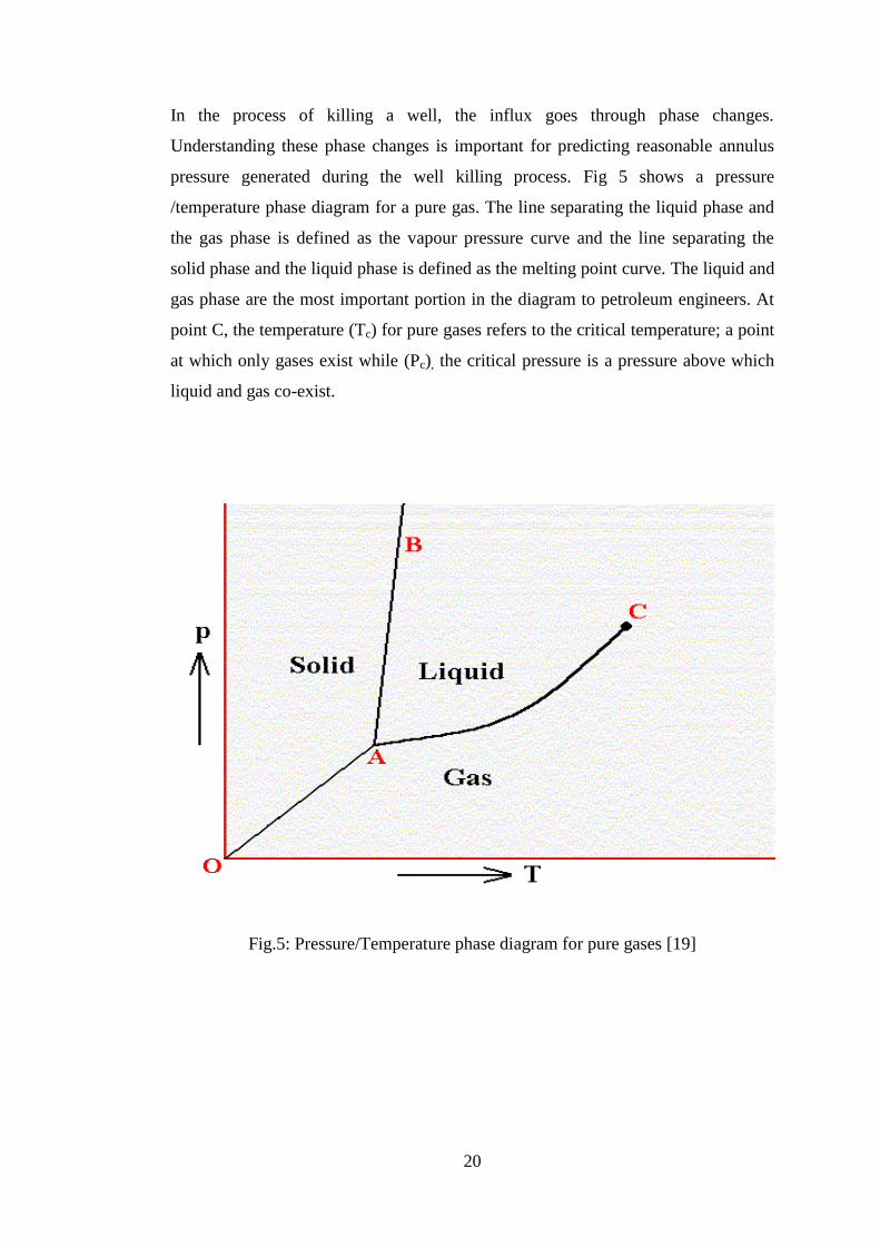
In the process of killing a well, the influx goes through phase changes.

Understanding these phase changes is important for predicting reasonable annulus

pressure generated during the well killing process. Fig 5 shows a pressure

/temperature phase diagram for a pure gas. The line separating the liquid phase and

the gas phase is defined as the vapour pressure curve and the line separating the

solid phase and the liquid phase is defined as the melting point curve. The liquid and

gas phase are the most important portion in the diagram to petroleum engineers. At

point C, the temperature (Tc) for pure gases refers to the critical temperature; a point

at which only gases exist while (Pc), the critical pressure is a pressure above which

liquid and gas co-exist.

Fig.5: Pressure/Temperature phase diagram for pure gases [19]

21

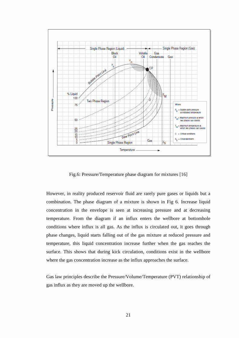
Fig.6: Pressure/Temperature phase diagram for mixtures [16]

However, in reality produced reservoir fluid are rarely pure gases or liquids but a

combination. The phase diagram of a mixture is shown in Fig 6. Increase liquid

concentration in the envelope is seen at increasing pressure and at decreasing

temperature. From the diagram if an influx enters the wellbore at bottomhole

conditions where influx is all gas. As the influx is circulated out, it goes through

phase changes, liquid starts falling out of the gas mixture at reduced pressure and

temperature, this liquid concentration increase further when the gas reaches the

surface. This shows that during kick circulation, conditions exist in the wellbore

where the gas concentration increase as the influx approaches the surface.

Gas law principles describe the Pressure/Volume/Temperature (PVT) relationship of

gas influx as they are moved up the wellbore.

22

Robert Boyle [19] found by experiment that at constant temperature, the volume of a

quantity of gas is inversely proportional to its pressure

……………………………………..Equation 8

Where,

P and V are the pressures and volumes of the gas at condition 1 and 2.

Charles [19] also found that the Temperature and Volume of a given quantity of gas

are direct proportional

……………………………………..Equation 9

Where,

V and T are volume and Temperature at condition 1 and 2.

Absolute Temperatures and Pressures are used in these equations

Another law, the Avogadro’s Law [19] states that under the same conditions of

temperature and pressure equal volumes of an ideal gas contains the same number of

molecules.

An equation of state for ideal gas is obtained by combining Boyle’s Law, Charles’s

Law with Avogadro’s Law, given as;

………………………………….Equation 10

Where,

P= Pressure

V= Volume

T= Temperature

n= Number of moles (mass divided by molecular weight)

Rg = Universal gas constant.

23

For an influx into the wellbore, n is constant, hence

…………………………………Equation 11

The gas density is given by mass per unit volume

…………………………………….Equation 12

Density of an ideal gas is given by

…………………………….Equation 13

Specific gravity for gas is given by the ration of its molecular weight to that of air

(Mg)

………………………………..Equation 14

From equation (13) and equation (14), Gas density is given by

………………………….Equation 15

Gas specific gravity is usually assumed between 0.6 and 0.7 for well control

purposes.

24

Ideal gas behavior was found to be valid only under limited range of pressure and

temperature conditions. For this reason compressibility factors or Z-Factors were

introduced to account for non-ideal gas behavior. The equation for non-ideal gas

behavior is given by

…………………………….Equation 16

The compressibility factors vary with changes in gas composition, temperature and

pressure. Z-Factors have been determined experimentally for various pure gases.

The curves in the plot have similar shapes but the actual Z values are component

specific. However, through the law of corresponding states all gases are shown to

have common values. The law of corresponding states, states that all pure gases

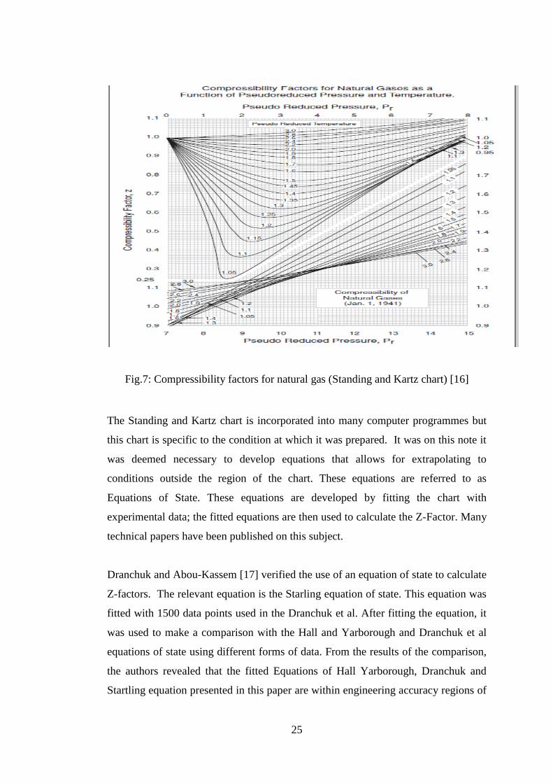
should have similar Z-Factor when the Pressure and Temperature are referenced to

the critical pressure and temperature of the gas. The reduced Temperature and

reduced Pressure makes this possible.

Reduced Temperature

…………………………Equation 17

Reduced Pressure

……………………………Equation 18

Where,

Tc = Critical Temperature

Pc = Critical Pressure

Having obtained the reduced temperature and reduced pressure, Z-Factors can be

obtained from the Standing and Kartz chart shown in Fig 7 [16].

25

Fig.7: Compressibility factors for natural gas (Standing and Kartz chart) [16]

The Standing and Kartz chart is incorporated into many computer programmes but

this chart is specific to the condition at which it was prepared. It was on this note it

was deemed necessary to develop equations that allows for extrapolating to

conditions outside the region of the chart. These equations are referred to as

Equations of State. These equations are developed by fitting the chart with

experimental data; the fitted equations are then used to calculate the Z-Factor. Many

technical papers have been published on this subject.

Dranchuk and Abou-Kassem [17] verified the use of an equation of state to calculate

Z-factors. The relevant equation is the Starling equation of state. This equation was

fitted with 1500 data points used in the Dranchuk et al. After fitting the equation, it

was used to make a comparison with the Hall and Yarborough and Dranchuk et al

equations of state using different forms of data. From the results of the comparison,

the authors revealed that the fitted Equations of Hall Yarborough, Dranchuk and

Startling equation presented in this paper are within engineering accuracy regions of

26

0.2 ≤ Pr ≤ 30, 1≤ Pr ≤ 3 and Pr≤ 1, 0,7 ≤ T ≤ 1 but are not accurate in the region Tr =

1; Pr≤ 1.

R.P Sutton [18] examined the effect of high molecular weight gases on the

calculation of compressibility factors and presented an equation for the calculation

of critical Temperature and critical Pressures for heptane plus gases. Compressibility

factors calculations are referenced to critical temperatures and pressures (single gas)

and pseudo-critical temperatures and pressures from Kay’s molar average

combination rules (gas mixtures). This rule gave inaccurate values for pseudo-

critical temperatures and pressures for heptane plus gases hence inaccurate Z-

factors. Using a data bank of laboratory measured natural gas composition and PVT

properties, it was found that the Lee-Kessler correlation gave more accurate results

and hence was recommended for calculating critical properties for heptane-plus

gases. The Stewart, Burkhardt and Voo (SBV) combination rules together with

empirical adjustments factors related to the presence of heptane plus greatly

improved the calculations of pseudo-critical temperatures and pressures and in

essence leading to a more accurate calculation of compressibility (Z) factor.

27

CHAPTER 3

METHODOLOGY

This chapter presents the methodology that will be used in this project to study the

effect of changes in geothermal temperature gradient and compressibility factor (Z-

Factor) in casing design. The study is done using excel macro programme.

The following algorithm will be adopted for the casing design using the kick

tolerance concept.

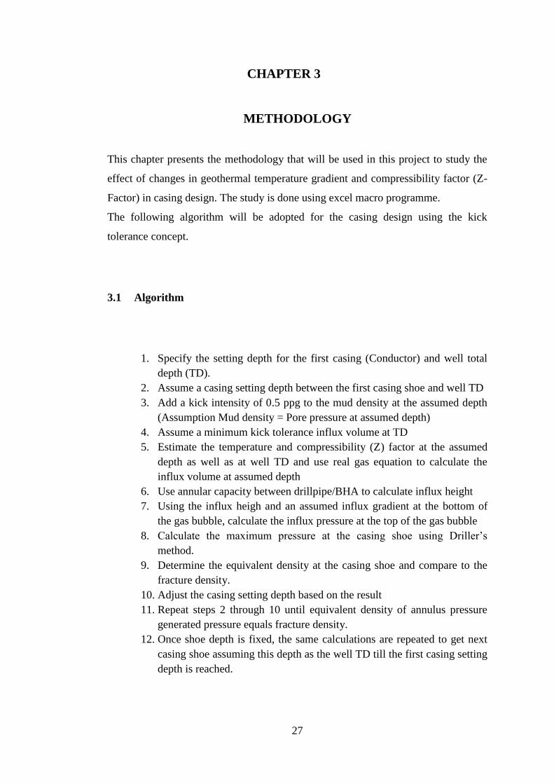
3.1 Algorithm

1. Specify the setting depth for the first casing (Conductor) and well total

depth (TD).

2. Assume a casing setting depth between the first casing shoe and well TD

3. Add a kick intensity of 0.5 ppg to the mud density at the assumed depth

(Assumption Mud density = Pore pressure at assumed depth)

4. Assume a minimum kick tolerance influx volume at TD

5. Estimate the temperature and compressibility (Z) factor at the assumed

depth as well as at well TD and use real gas equation to calculate the

influx volume at assumed depth

6. Use annular capacity between drillpipe/BHA to calculate influx height

7. Using the influx heigh and an assumed influx gradient at the bottom of

the gas bubble, calculate the influx pressure at the top of the gas bubble

8. Calculate the maximum pressure at the casing shoe using Driller’s

method.

9. Determine the equivalent density at the casing shoe and compare to the

fracture density.

10. Adjust the casing setting depth based on the result

11. Repeat steps 2 through 10 until equivalent density of annulus pressure

generated pressure equals fracture density.

12. Once shoe depth is fixed, the same calculations are repeated to get next

casing shoe assuming this depth as the well TD till the first casing setting

depth is reached.

28

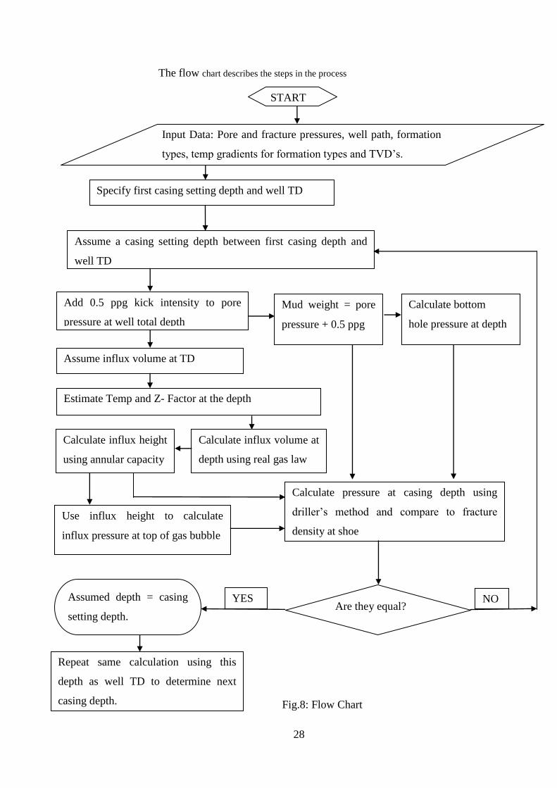
The flow chart describes the steps in the process

Fig.8: Flow Chart

START

Input Data: Pore and fracture pressures, well path, formation

types, temp gradients for formation types and TVD’s.

Specify first casing setting depth and well TD

Assume a casing setting depth between first casing depth and

well TD

Add 0.5 ppg kick intensity to pore

pressure at well total depth

Mud weight = pore

pressure + 0.5 ppg

Calculate bottom

hole pressure at depth

Assume influx volume at TD

Estimate Temp and Z- Factor at the depth

Calculate influx volume at

depth using real gas law

Calculate influx height

using annular capacity

Use influx height to calculate

influx pressure at top of gas bubble

Calculate pressure at casing depth using

driller’s method and compare to fracture

density at shoe

Are they equal? YES NO

R

e

p

e

a

t

Assumed depth = casing

setting depth.

Repeat same calculation using this

depth as well TD to determine next

casing depth.

29

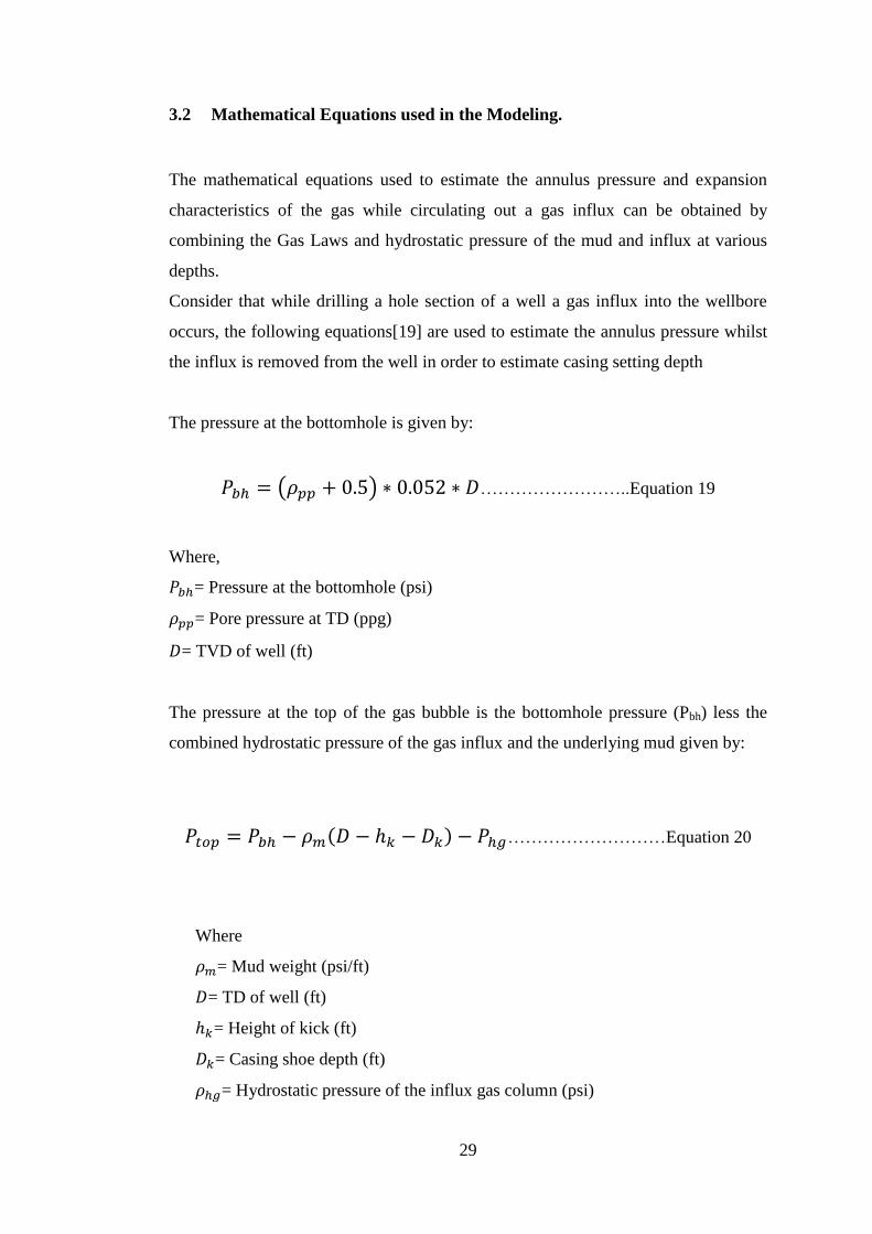
3.2 Mathematical Equations used in the Modeling.

The mathematical equations used to estimate the annulus pressure and expansion

characteristics of the gas while circulating out a gas influx can be obtained by

combining the Gas Laws and hydrostatic pressure of the mud and influx at various

depths.

Consider that while drilling a hole section of a well a gas influx into the wellbore

occurs, the following equations[19] are used to estimate the annulus pressure whilst

the influx is removed from the well in order to estimate casing setting depth

The pressure at the bottomhole is given by:

( ) ……………………..Equation 19

Where,

= Pressure at the bottomhole (psi)

= Pore pressure at TD (ppg)

= TVD of well (ft)

The pressure at the top of the gas bubble is the bottomhole pressure (Pbh) less the

combined hydrostatic pressure of the gas influx and the underlying mud given by:

………………………Equation 20

Where

= Mud weight (psi/ft)

= TD of well (ft)

= Height of kick (ft)

= Casing shoe depth (ft)

= Hydrostatic pressure of the influx gas column (psi)

30

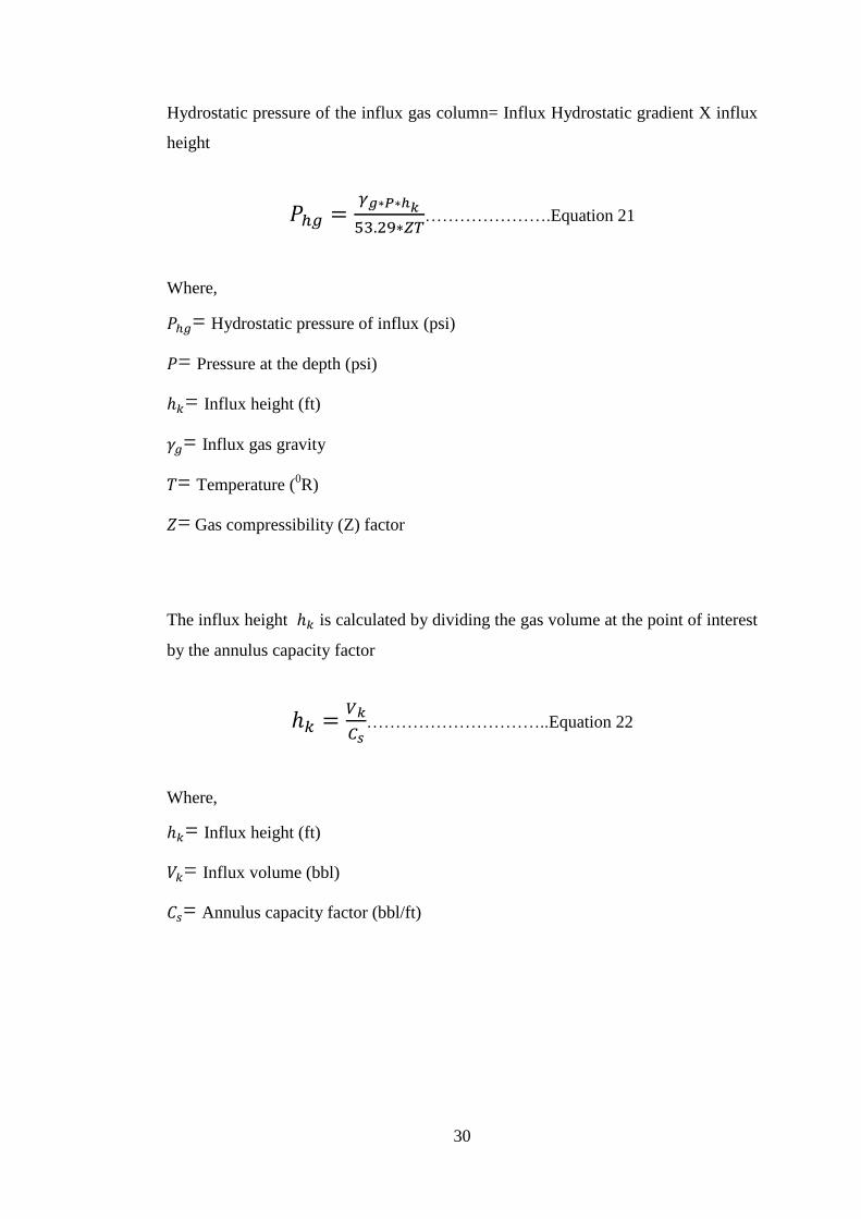
Hydrostatic pressure of the influx gas column= Influx Hydrostatic gradient X influx

height

………………….Equation 21

Where,

= Hydrostatic pressure of influx (psi)

= Pressure at the depth (psi)

= Influx height (ft)

= Influx gas gravity

= Temperature (0R)

= Gas compressibility (Z) factor

The influx height is calculated by dividing the gas volume at the point of interest

by the annulus capacity factor

…………………………..Equation 22

Where,

= Influx height (ft)

= Influx volume (bbl)

= Annulus capacity factor (bbl/ft)

31

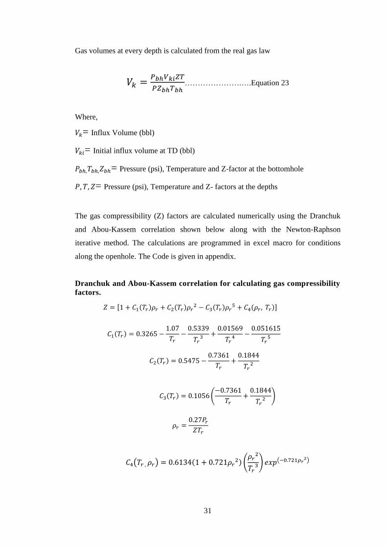
Gas volumes at every depth is calculated from the real gas law

………………….….Equation 23

Where,

= Influx Volume (bbl)

= Initial influx volume at TD (bbl)

= Pressure (psi), Temperature and Z-factor at the bottomhole

= Pressure (psi), Temperature and Z- factors at the depths

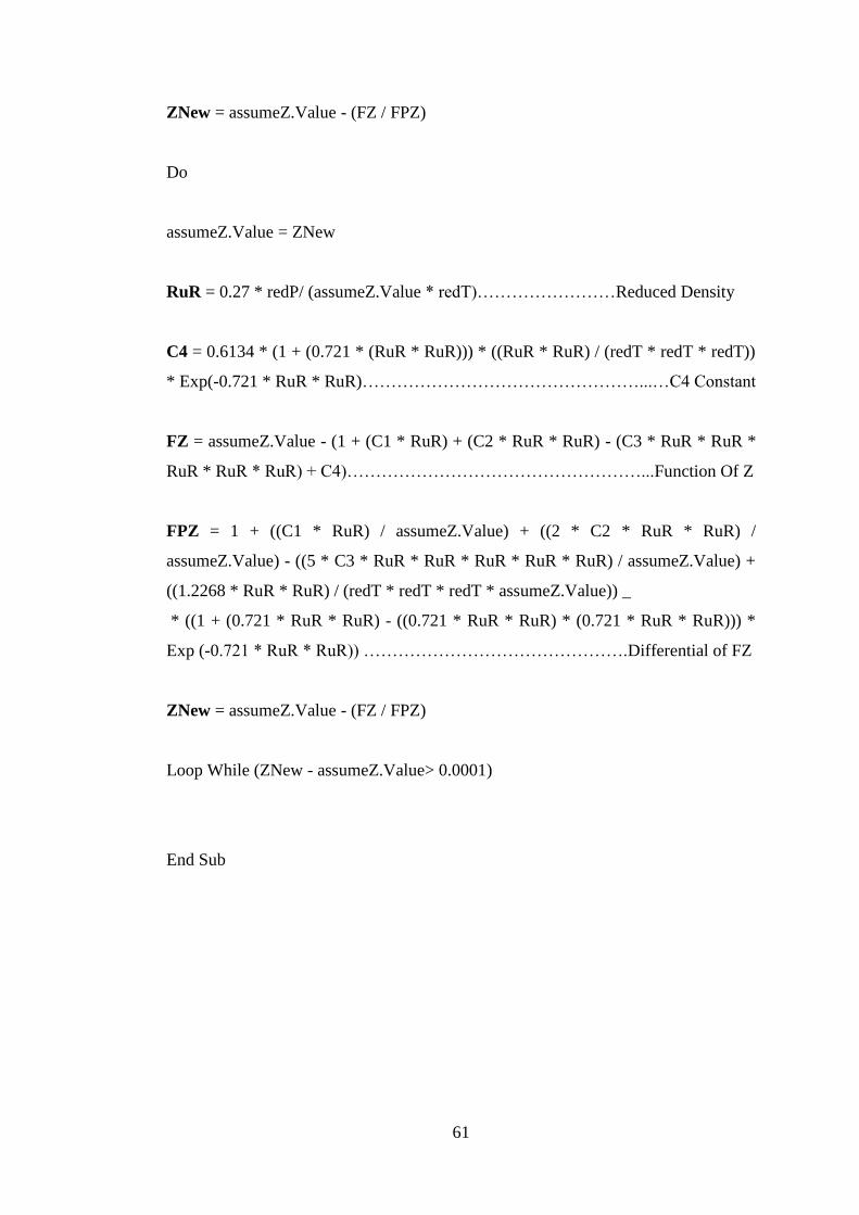
The gas compressibility (Z) factors are calculated numerically using the Dranchuk

and Abou-Kassem correlation shown below along with the Newton-Raphson

iterative method. The calculations are programmed in excel macro for conditions

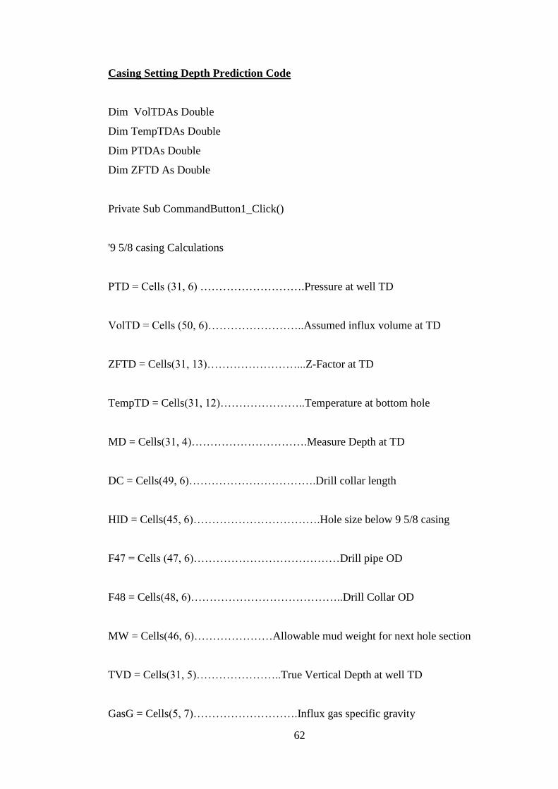
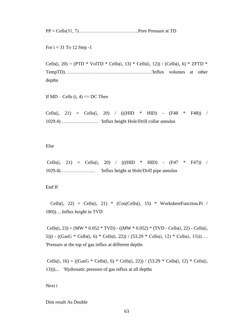
along the openhole. The Code is given in appendix.

Dranchuk and Abou-Kassem correlation for calculating gas compressibility

factors.

[

]

(

)

( ) (

) (

)

32

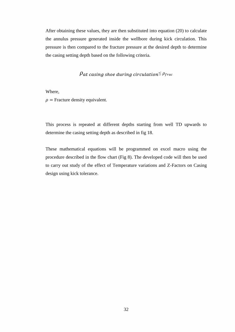
After obtaining these values, they are then substituted into equation (20) to calculate

the annulus pressure generated inside the wellbore during kick circulation. This

pressure is then compared to the fracture pressure at the desired depth to determine

the casing setting depth based on the following criteria.

≤

Where,

Fracture density equivalent.

This process is repeated at different depths starting from well TD upwards to

determine the casing setting depth as described in fig 18.

These mathematical equations will be programmed on excel macro using the

procedure described in the flow chart (Fig 8). The developed code will then be used

to carry out study of the effect of Temperature variations and Z-Factors on Casing

design using kick tolerance.

33

CHAPTER 4

ANALYSIS, RESULTS AND DISCUSSIONS

This chapter contains the analysis done on the project in order to achieve the

objectives. It also presents the results and discusses their significance.

4.1 Model Input Data

To account for the kick tolerance in casing setting depth selection for an oil well,

the following data are required:

1. The well geometry, comprising of the MD, inclinations and TVD.

2. The formation pressure at TD of the hole section considered.

3. The mud weights for the next hole section

4. The maximum kick volumes that can be circulated out

5. The fracture equivalent density curve of the formation.

The data used for the analysis is from a real field well. It is a deviated well with a

build- up rate of 30/100ft and a final inclination angle of 77.69

0. The MD of the well

is 15653 ft. with a corresponding TVD of 5404 ft. The well trajectory is given in Fig

9.

A summary of the hole sizes, casing sizes and mud weights of the well use in the

simulation is given in Table 1. The table also gives the mud weights used in the

different hole sections.

Table 1: Well Parameters for Simulation

Wellbore Diameter

(in)

Casing Sizes

(in)

DrillCollar OD

(in)

DrillPipe OD

(in)

Mud weight

(ppg)

12.25 13.375 9 5 11.75

8.5 9.625 6.25 5 10.7

34

Fig.9: Well Trajectory

35

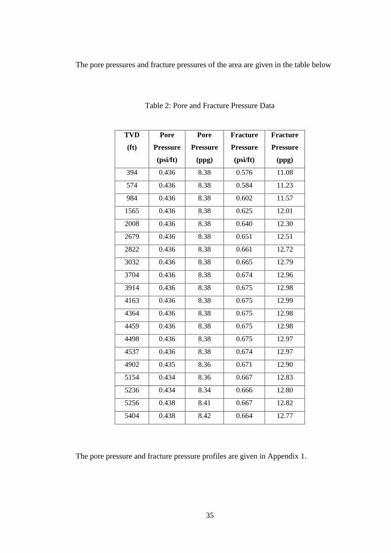
The pore pressures and fracture pressures of the area are given in the table below

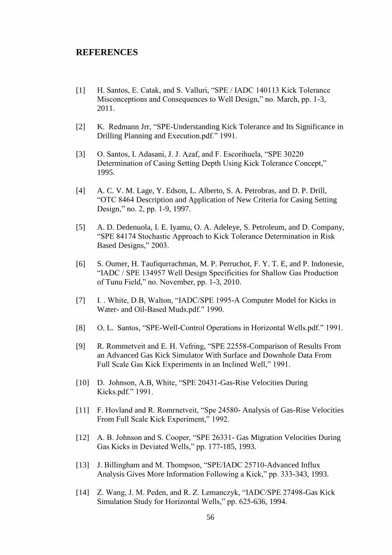
Table 2: Pore and Fracture Pressure Data

TVD

(ft)

Pore

Pressure

(psi/ft)

Pore

Pressure

(ppg)

Fracture

Pressure

(psi/ft)

Fracture

Pressure

(ppg)

394 0.436 8.38 0.576 11.08

574 0.436 8.38 0.584 11.23

984 0.436 8.38 0.602 11.57

1565 0.436 8.38 0.625 12.01

2008 0.436 8.38 0.640 12.30

2679 0.436 8.38 0.651 12.51

2822 0.436 8.38 0.661 12.72

3032 0.436 8.38 0.665 12.79

3704 0.436 8.38 0.674 12.96

3914 0.436 8.38 0.675 12.98

4163 0.436 8.38 0.675 12.99

4364 0.436 8.38 0.675 12.98

4459 0.436 8.38 0.675 12.98

4498 0.436 8.38 0.675 12.97

4537 0.436 8.38 0.674 12.97

4902 0.435 8.36 0.671 12.90

5154 0.434 8.36 0.667 12.83

5236 0.434 8.34 0.666 12.80

5256 0.438 8.41 0.667 12.82

5404 0.438 8.42 0.664 12.77

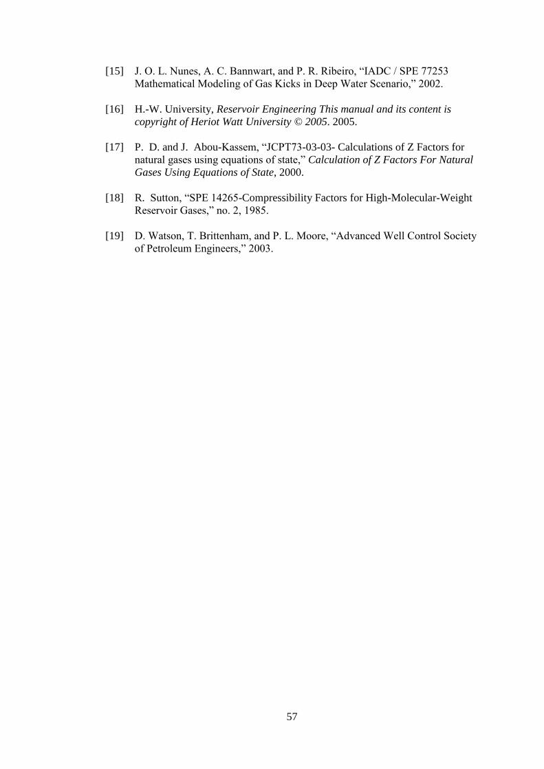
The pore pressure and fracture pressure profiles are given in Appendix 1.

36

4.2 Study Cases

In order to achieve the main objective of the study, that is to study the effect of

formations geothermal variations and Z-Factors on selection of casing setting

depths, four cases are studied.

CASE 1: Constant geothermal gradient and ideal gas behavior (Z=1) which is the

normal industry practice.

CASE 2: Constant Geothermal Gradient and real gas behavior (Effect of Z-Factor)

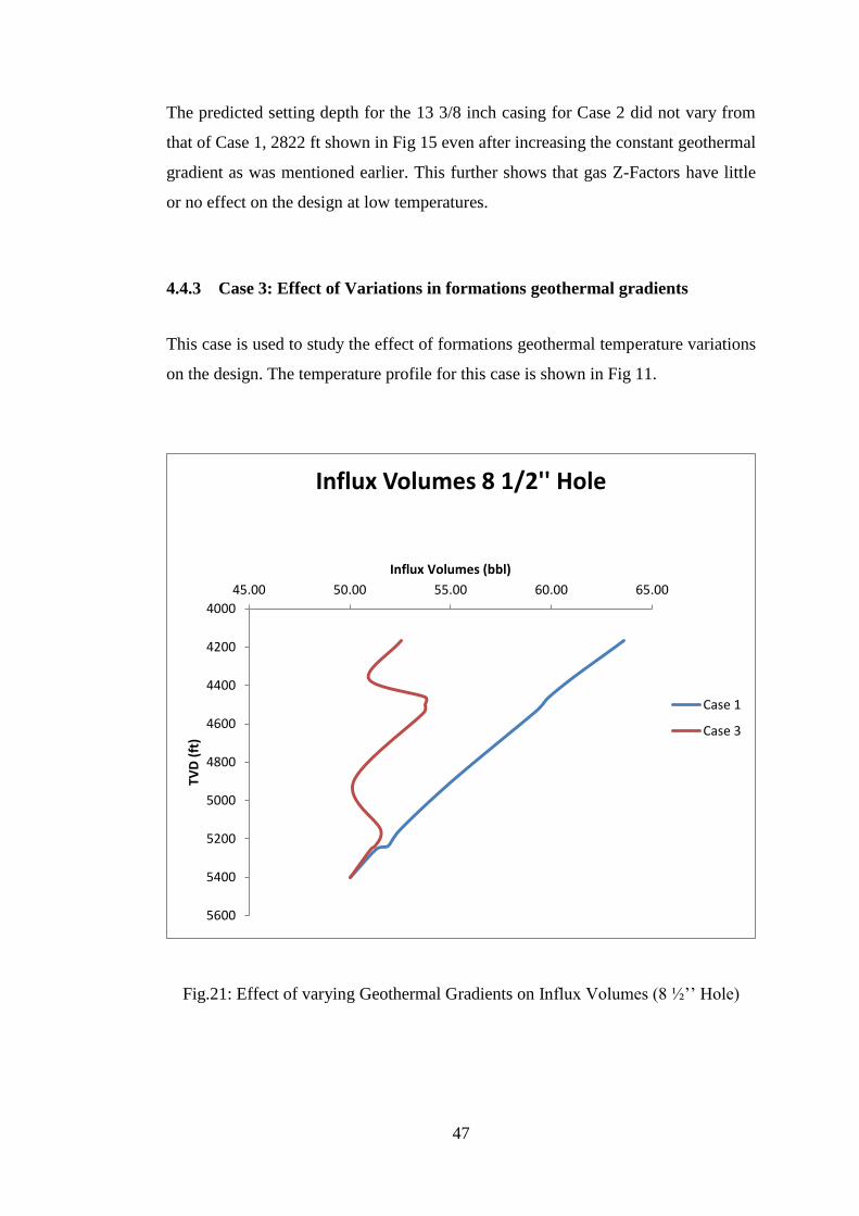
The temperature profile for case 1 and case 2 is given in Fig 10.

CASE 3: Varying Geothermal gradients across formations and ideal gas behavior

(Effect of Varying Geothermal gradient (Z=1)).

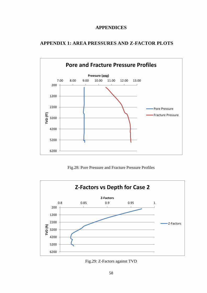
CASE 4: Varying geothermal gradients across formations and real gas behavior

(Effect of varying of varying geothermal gradients and Z-Factor).

The temperature profile for Cases 3 and 4 is given in Fig 11.

Prediction of the setting depths for casing is done for all the cases mentioned above

using a casing setting depth code programmed on excel macro as described in the

methodology chapter.

The procedure involves calculating the internal wellbore pressure generated when

circulating out a gas influx from a well at various depths. The density equivalent of

the calculated pressure is plotted on the same graph with the fracture gradient of the

area in order to determine the setting depth which is the point of intersection of both

curves.

37

Methane gas of 0.6 S.G, critical pressure of 667.8 psi and critical temperature of

3430R is assumed to be the influx gas. The other simplifying assumptions used in

carrying out the calculations are given below:

1. Influx enters the well and resides in the annulus as a slug of gas.

2. Influx does not mix with mud i.e it remains as a slug during circulation.

3. Free influx gas does not slip or migrate through a circulating or static mud

column.

4. The influx is a consistent fluid in one phase

5. No free gas dissolves in the mud

6. Annulus friction losses are negligible

7. The influx does not change phases during the displacement process

.

All depths used in the hydrostatic calculations are True Vertical Depths (TVD).

The Z-Factors along the borehole wall for the different temperature profiles are

calculated using the Abou-Kaseem and Dranchuk correlation combined with

Newton-Raphson iterative method. This was programmed on Excel Macro. The

code is given in Appendix 2.

38

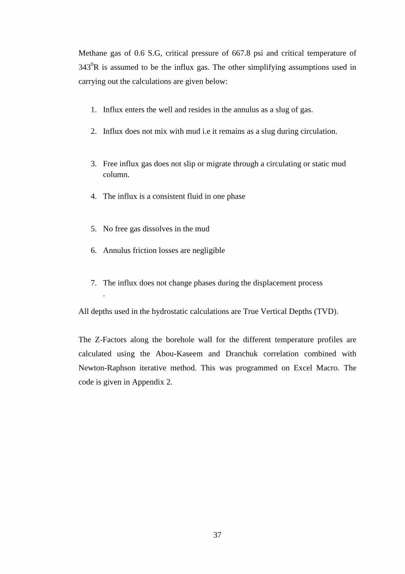
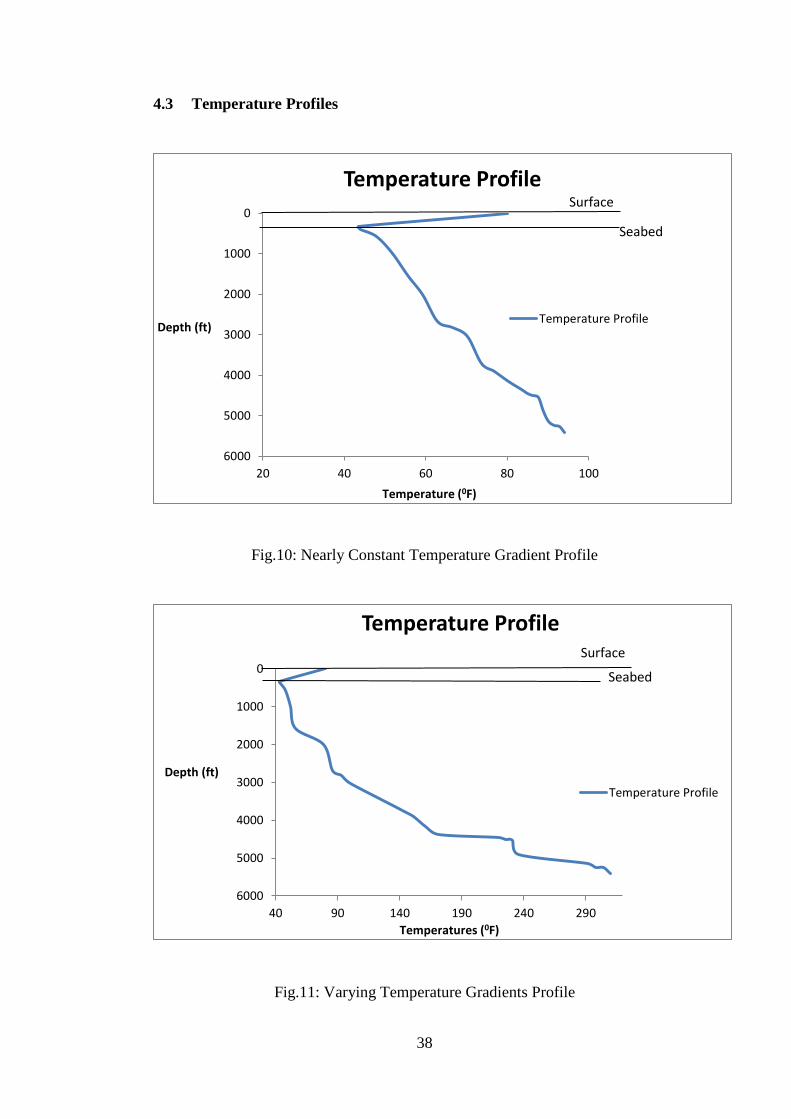
4.3 Temperature Profiles

Fig.10: Nearly Constant Temperature Gradient Profile

Fig.11: Varying Temperature Gradients Profile

0

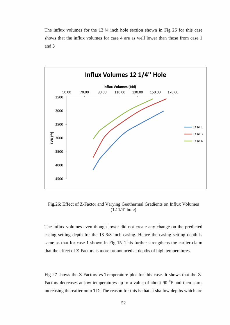
1000

2000

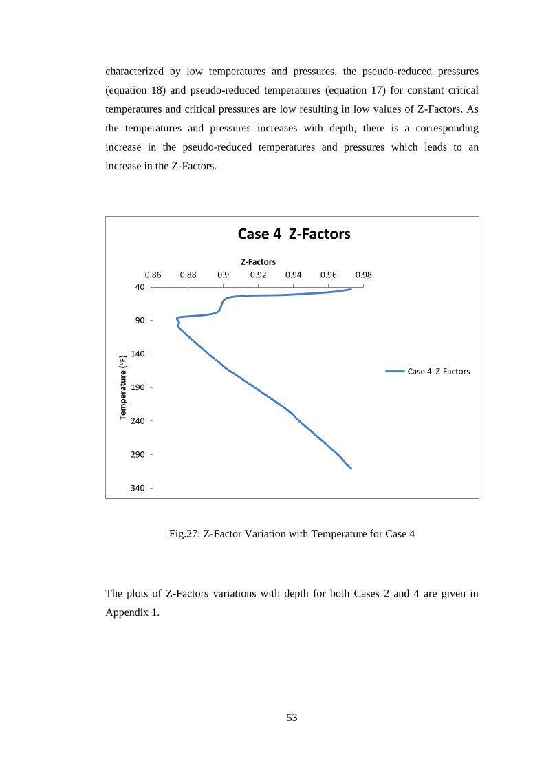
3000

4000

5000

6000

20 40 60 80 100

Depth (ft)

Temperature (0F)

Temperature Profile

Temperature Profile

Seabed

Surface

0

1000

2000

3000

4000

5000

6000

40 90 140 190 240 290

Depth (ft)

Temperatures (0F)

Temperature Profile

Temperature Profile

Seabed

Surface

39

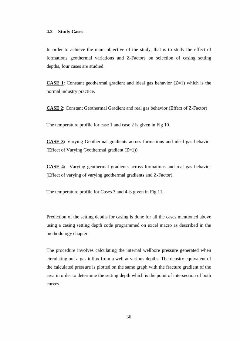
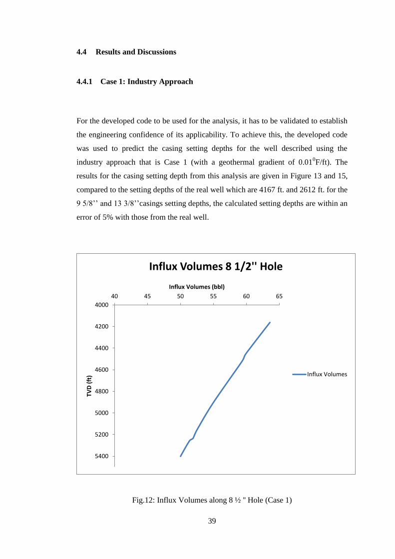
4.4 Results and Discussions

4.4.1 Case 1: Industry Approach

For the developed code to be used for the analysis, it has to be validated to establish

the engineering confidence of its applicability. To achieve this, the developed code

was used to predict the casing setting depths for the well described using the

industry approach that is Case 1 (with a geothermal gradient of 0.010F/ft). The

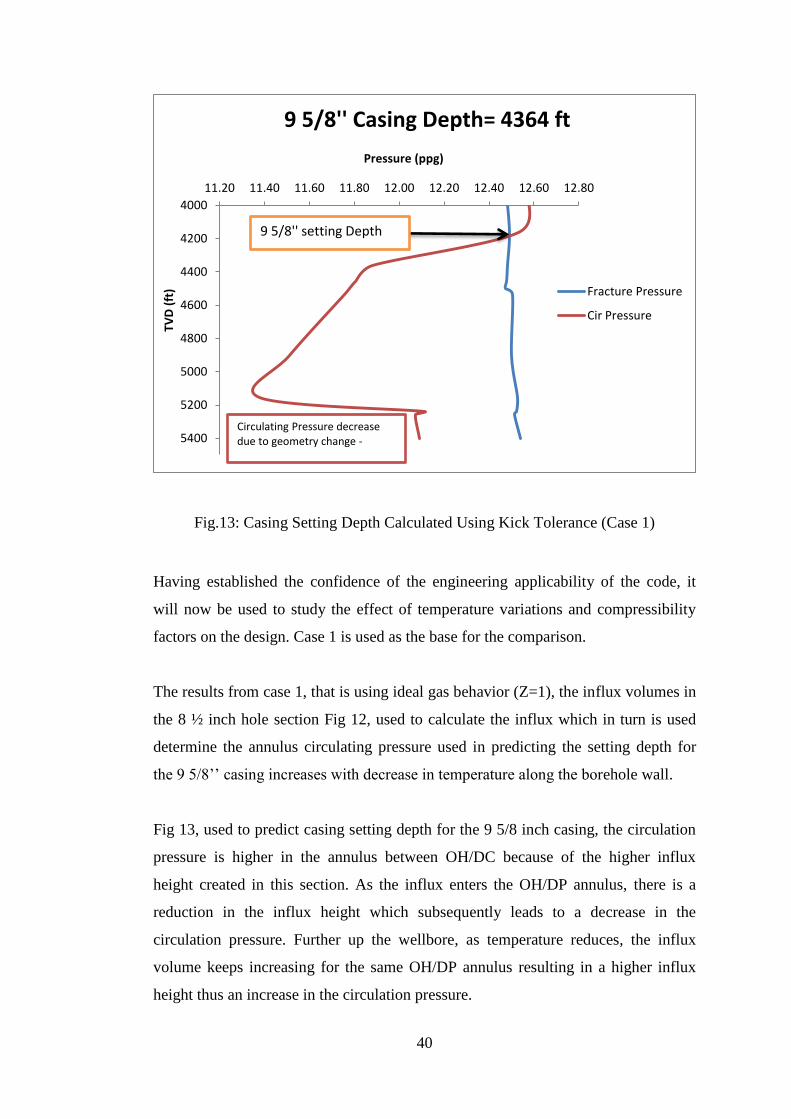
results for the casing setting depth from this analysis are given in Figure 13 and 15,

compared to the setting depths of the real well which are 4167 ft. and 2612 ft. for the

9 5/8’’ and 13 3/8’’casings setting depths, the calculated setting depths are within an

error of 5% with those from the real well.

Fig.12: Influx Volumes along 8 ½ '' Hole (Case 1)

4000

4200

4400

4600

4800

5000

5200

5400

40 45 50 55 60 65

TVD

(ft

)

Influx Volumes (bbl)

Influx Volumes 8 1/2'' Hole

Influx Volumes

40

Fig.13: Casing Setting Depth Calculated Using Kick Tolerance (Case 1)

Having established the confidence of the engineering applicability of the code, it

will now be used to study the effect of temperature variations and compressibility

factors on the design. Case 1 is used as the base for the comparison.

The results from case 1, that is using ideal gas behavior (Z=1), the influx volumes in

the 8 ½ inch hole section Fig 12, used to calculate the influx which in turn is used

determine the annulus circulating pressure used in predicting the setting depth for

the 9 5/8’’ casing increases with decrease in temperature along the borehole wall.

Fig 13, used to predict casing setting depth for the 9 5/8 inch casing, the circulation

pressure is higher in the annulus between OH/DC because of the higher influx

height created in this section. As the influx enters the OH/DP annulus, there is a

reduction in the influx height which subsequently leads to a decrease in the

circulation pressure. Further up the wellbore, as temperature reduces, the influx

volume keeps increasing for the same OH/DP annulus resulting in a higher influx

height thus an increase in the circulation pressure.

4000

4200

4400

4600

4800

5000

5200

5400

11.20 11.40 11.60 11.80 12.00 12.20 12.40 12.60 12.80

TVD

(ft

) Pressure (ppg)

9 5/8'' Casing Depth= 4364 ft

Fracture Pressure

Cir Pressure

Circulating Pressure decrease due to geometry change -

9 5/8'' setting Depth

41

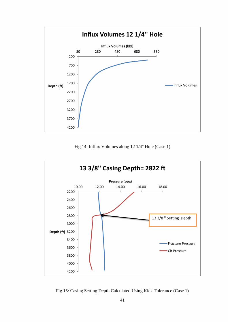
Fig.14: Influx Volumes along 12 1/4'' Hole (Case 1)

Fig.15: Casing Setting Depth Calculated Using Kick Tolerance (Case 1)

200

700

1200

1700

2200

2700

3200

3700

4200

80 280 480 680 880

Depth (ft)

Influx Volumes (bbl)

Influx Volumes 12 1/4'' Hole

Influx Volumes

2200

2400

2600

2800

3000

3200

3400

3600

3800

4000

4200

10.00 12.00 14.00 16.00 18.00

Depth (ft)

Pressure (ppg)

13 3/8'' Casing Depth= 2822 ft

Fracture Pressure

Cir Pressure

13 3/8 '' Setting Depth

42

For the 12 ¼ inch hole which starts at the shoe of the 13 3/8 inch casing and ends at

the 9 5/8 inch casing, Fig 14 shows the trend of the influx volumes along the open

hole. The influx volumes increases as influx migrates up the wellbore where there is

a decrease in temperatures. The influx volumes increase is significant at very low

temperatures which are found at shallow depths.

In Fig 15 used to estimate the casing setting depth, the same argument put forward

for the 9 5/8 inch casing is valid here as well but only that the decrease in the

circulation pressure at the OH/DP annulus is not as evident as that for the 9 5/8 inch

casing. This is probably due to the higher influx volumes that have resulted because

of the low temperatures at these depths.

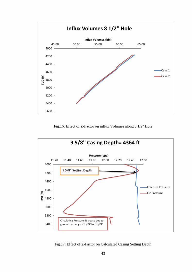
4.4.2 Case 2: Effect of Gas Compressibility (Z) Factor

This case is used to study the effect of the gas compressibility (Z) Factor on the

design. The Z-Factor for the temperatures and pressures at every depth along the

borehole is calculated using Abou-Kassem and Dranchuk correlation assuming

Methane gas of 0.6 S.G as the influx fluid

Gas compressibility factor, is a parameter that allows for using the ideal gas

equation to model real gas behavior.

43

Fig.16: Effect of Z-Factor on influx Volumes along 8 1/2'' Hole

Fig.17: Effect of Z-Factor on Calculated Casing Setting Depth

4000

4200

4400

4600

4800

5000

5200

5400

5600

45.00 50.00 55.00 60.00 65.00TV

D (

ft)

Influx Volumes (bbl)

Influx Volumes 8 1/2'' Hole

Case 1

Case 2

4000

4200

4400

4600

4800

5000

5200

5400

11.20 11.40 11.60 11.80 12.00 12.20 12.40 12.60

TVD

(ft

)

Pressure (ppg)

9 5/8'' Casing Depth= 4364 ft

Fracture Pressure

Cir Pressure

Circulating Pressure decrease due to geometry change -OH/DC to OH/DP

9 5/8'' Setting Depth

44

Using real gas equation to model the influx gas behaviour, the influx volumes in the

8 ½ inch hole section increases with decrease in temperature along the borehole wall

just like in case 1 but the influx volumes are lower than those from case 1 as shown

in Fig 16.

The predicted setting depth for the 9 5/8 inch casing Fig 17 for case 2 did not change

from that of case 1 even though there is a difference in volume between case 1 and

case 2. The Z-Factors for case 2 decreases at low temperatures, later it starts

increasing at temperatures higher than 90 0F as shown in Fig 18.

Fig.18: Z-Factor Variation with Temperature (Case 2)

The decrease in Z-Factors along the borehole wall with reference to the Z-Factors at

TD for the 8 ½ inch hole have resulted in lower volumes for this case as compared

to case 1 where the Z-Factors are constant throughout. This change is significant

because it shows that for the same casing setting depth, the kick tolerance when Z-

Factors are included in the calculations will be higher than when it is ignored.

40

50

60

70

80

90

100

0.8 0.85 0.9 0.95 1

Tem

pe

ratu

re (

oF)

Z-Factors

Case 2 Z-Factors

Case 2 Z-Factors

45

Another significance it shows is that for HT/HP wells where the window between

Pore pressure and fracture pressure is small, the inclusion of Z-Factors in the

calculations reduces the risk of fracturing the weakest formation during influx

circulation.

Fig.19: Effect of Increase in Geothermal Gradients on Influx Volumes

Fig 19 above shows the variation in influx volumes at the 8 ½ inch hole when the

constant geothermal temperature gradient is 0.01 0

F/ft, 0.015 0F/ft and 0.02

0F/ft for

both case 1 and Case 2. It is evident that the difference in influx volumes between

case 1 and 2 is wider at a constant geothermal temperature gradient of 0.02 0F/ft. In

fact when this temperature gradient was used for the analysis, the setting depth in

case 2 was found to be 4163 ft. which is 201 ft. shallower than that for the same

temperature gradient used in Case 1 (Z=1). This shows that at increased bottomhole

4000

4200

4400

4600

4800

5000

5200

5400

5600

45.00 50.00 55.00 60.00 65.00

TVD

(ft

)

Influx Volumes (bbl)

Influx Volumes 8 1/2'' Hole

Case 1 geothermal gradient0.01F/ft

Case 2 geothermal gradient0.01F/ft

Case 1 geothermal gradient0.015F/ft

Case 2 geothermal gradient0.015F/ft

Case 1 geothermal gradient0.02F/ft

Case 2 geothermal gradient0.02F/ft

46

temperatures, the Z-Factors have an effect on the predicted casing setting depth.

This further highlights the significance of the Z-Factor inclusion in the calculation

especially for HT/HP wells where the correction for Z-Factor in the calculations

gives lower gas influx volumes along the borehole wall during circulation, thereby

reducing the risk of fracturing the weakest formation.

On the other side if the influx volumes in the calculations is not corrected for Z-

Factors, there is a high risk that the fracture pressure of the weakest formation will

be exceeded during circulation because of the high influx volumes generated.

Fig.20: Influx Volumes 12 1/4 '' hole for Case 1 and Case 2

For the 12 ¼ inch hole section in case 2, the influx volumes curve is similar to that

obtained for case 1 (Fig 14) but the absolute values are greater than those from case

1 as shown in Fig 20. This is because influx volumes increase as the Z-Factors with

respect to the Z-Factor at TD increase along the wellbore as seen in Fig 18.

2000

2500

3000

3500

4000

4500

50.00 70.00 90.00 110.00 130.00 150.00 170.00 190.00

TVD

(ft

)

Influx Volumes (bbl)

Influx Volumes 12 1/4'' Hole

Case 1

Case 2

47

The predicted setting depth for the 13 3/8 inch casing for Case 2 did not vary from

that of Case 1, 2822 ft shown in Fig 15 even after increasing the constant geothermal

gradient as was mentioned earlier. This further shows that gas Z-Factors have little

or no effect on the design at low temperatures.

4.4.3 Case 3: Effect of Variations in formations geothermal gradients

This case is used to study the effect of formations geothermal temperature variations

on the design. The temperature profile for this case is shown in Fig 11.

Fig.21: Effect of varying Geothermal Gradients on Influx Volumes (8 ½’’ Hole)

4000

4200

4400

4600

4800

5000

5200

5400

5600

45.00 50.00 55.00 60.00 65.00

TVD

(ft

)

Influx Volumes (bbl)

Influx Volumes 8 1/2'' Hole

Case 1

Case 3

48

Fig.22: Effect of Varying Geothermal Gradients on Calculated Setting Depth

For this case, the influx volumes in the 8 ½ inch hole section are lower compared to

those from case 1 as shown in Fig 21. The influx volumes in case 3 increase from

TD moving up the wellbore but decreases at the transition between formations of

different geothermal gradients.

The increase in temperature in case 3 is believed to be responsible for the reduction

in the influx volumes as compared to case 1 which has lower temperatures for this

hole section.

Because of this, the casing setting depth predicted in case 3 shown in Fig 22 is found

to be 3914 ft. which is 450 ft. shallower than that obtained from case 1. This is

expected because at lower influx volumes which translates to a lower influx height

for the same hole size and BHA, the length of open hole section that can be drilled

safely without fracturing the weakest formation at shoe when circulating out a gas

3000

3500

4000

4500

5000

5500

11.20 11.40 11.60 11.80 12.00 12.20 12.40 12.60 12.80TV

D (

ft)

Pressure (ppg)

9 5/8'' Casing Depth= 3914 ft

Fracture Pressure

Cir Pressure

Cir Pressure decrease due to geometry change -OH/DC to OH/DP

9 5/8'' Setting Depth

49

influx will be greater than when the influx volumes are higher. Hence, the increase

in geothermal gradient leads to reduced influx volumes during circulation compared

to Case 1 there by giving a shallower predicted setting depth for the 9 5/8 inch

casing.

Fig.23: Effect of Varying Geothermal Gradients on Influx volumes (12 1/4'' hole)

For the 12 ¼ inch hole section, the influx volumes increases as it moves up the

wellbore from TD. But unlike the 8 ½ inch hole, the volumes curve for this hole

section did not show any abrupt change between formation of varying geothermal

gradients. This is probably due to the fact that temperatures at these depths are

lower. The volumes for this case is lower than those from case 1 for the same hole

section as shown in Fig 23.

Even though there is a difference in influx volumes at this hole section between case

1 and case 3, the volume changes did not result in any change for the predicted 13

3/8 inch casing shoe depth from that obtained for case 1 shown in Fig 15. This

1500

2000

2500

3000

3500

4000

4500

50.00 70.00 90.00 110.00 130.00 150.00 170.00

TVD

(ft

)

Influx Volumes (bbl)

Influx Volumes 12 1/4'' Hole

Case 1

Case 3

50

discovery shows that at shallow depths, variation in formation geothermal gradients

does not have a significant impact on the setting depth prediction. This is probably

due to the fact that at shallow depths variation in geothermal gradients does not lead

to significant change in temperatures from those of constant geothermal gradients.

4.4.4 Case 4: Effect of varying geothermal gradients and Z-Factor

This case is used to study the effect of real gas behavior on the design of case 3

when the temperature profile of Fig 11 is used. For this case just like in case 2, the

gas compressibility factors for every pressure and temperature at every depth is

calculated using the Abou-kaseem and Dranchuk correlation combined with the

Newton-Raphson iterative method.

Fig.24: Effect of Z-factor and Varying Geothermal Gradient on Influx Volumes (8

1/2'' hole)

2500

3000

3500

4000

4500

5000

5500

6000

45.00 50.00 55.00 60.00 65.00

TVD

(ft

)

Influx Volumes (bbl)

Influ Volumes 8 1/2'' Hole

Case 1

Case 3

Case 4

51

Fig.25: Effect of Z-Factor and Varying Geothermal Gradient on Calculated Casing

Setting Depth.

The influx volumes along the 81/2 inch hole section in Fig 24, used to estimate the

setting depth for the 9 5/8 inch casing shoe has a curve similar to that obtained in

case 3 but with lower influx volumes as compared to case 1 and case 3. The

reduction in influx volumes is as a result of decrease in the Z-Factors for this case,

unlike in cases 1 and 3 were the Z-Factors remains constant throughout.

The 9 5/8 inch casing setting depth predicted for this case Fig 25 is shallower than

those obtained for case 1 and case 3. This is expected because of the lower influx

volumes generated during influx circulation as was explained earlier in case 3.

2800

3300

3800

4300

4800

5300

11.20 11.40 11.60 11.80 12.00 12.20 12.40 12.60TV

D (

ft)

Pressure (ppg)

9 5/8'' Casing Depth= 3704 ft

Fracture Pressure

Cir Pressure

Cir Pressure decrease due to geometry change -OH/DC to OH/DP

9 5/8'' Setting Depth

52

The influx volumes for the 12 ¼ inch hole section shown in Fig 26 for this case

shows that the influx volumes for case 4 are as well lower than those from case 1

and 3

Fig.26: Effect of Z-Factor and Varying Geothermal Gradients on Influx Volumes

(12 1/4'' hole)

The influx volumes even though lower did not create any change on the predicted

casing setting depth for the 13 3/8 inch casing. Hence the casing setting depth is

same as that for case 1 shown in Fig 15. This further strengthens the earlier claim

that the effect of Z-Factors is more pronounced at depths of high temperatures.

Fig 27 shows the Z-Factors vs Temperature plot for this case. It shows that the Z-

Factors decreases at low temperatures up to a value of about 90 0F and then starts

increasing thereafter onto TD. The reason for this is that at shallow depths which are

1500

2000

2500

3000

3500

4000

4500

50.00 70.00 90.00 110.00 130.00 150.00 170.00

TVD

(ft

)

Influx Volumes (bbl)

Influx Volumes 12 1/4'' Hole

Case 1

Case 3

Case 4

53

characterized by low temperatures and pressures, the pseudo-reduced pressures

(equation 18) and pseudo-reduced temperatures (equation 17) for constant critical

temperatures and critical pressures are low resulting in low values of Z-Factors. As

the temperatures and pressures increases with depth, there is a corresponding

increase in the pseudo-reduced temperatures and pressures which leads to an

increase in the Z-Factors.

Fig.27: Z-Factor Variation with Temperature for Case 4

The plots of Z-Factors variations with depth for both Cases 2 and 4 are given in

Appendix 1.

40

90

140

190

240

290

340

0.86 0.88 0.9 0.92 0.94 0.96 0.98

Tem

pe

ratu

re (

oF)

Z-Factors

Case 4 Z-Factors

Case 4 Z-Factors

54

CHAPTER 5

CONCLUSIONS AND RECOMMENDATIONS

5.1 Conclusions

In this study, it has been shown that:

1. Correcting for Z-Factors in the calculation of influx volumes results in lower

influx volumes compared to those obtained from the industry approach

where Z-Factors are ignored. This implies that correcting for Z-Factors

reduces the risk of fracturing the weakest formation during influx

circulations. This is particularly important when dealing with HT/HP wells

where the window between pore pressure and fracture pressure is narrow.

2. For the same Casing Setting depth and hole section, Z-Factor corrected

calculations gives a higher kick tolerance than that obtained when Z-Factors

are ignored. For conventional wells, this means that longer hole sections can

be drilled safely before running casing. This reduces the casing strings to be

run in the well, consequently reducing the well cost.

3. Z-Factors have little or no effect on the prediction of casing setting depth at

low temperatures and pressures, but become very significant at very high

temperatures and pressures. This is because of the large difference in influx

volumes between the real gas behavior case (Z-Factor corrected for) and

ideal gas case (Z=1)

4. Accounting for variations in geothermal gradients across subsurface

formations results in lower influx volumes than those obtained when a

constant formation geothermal gradient is used in the calculations.

5. Casing setting depth prediction is affected by high temperatures. This

conclusion was arrived at when variations in geothermal gradient was

accounted for, the setting depth for casing at depths of very high

temperatures gave a shallower predicted depth than that obtained for the

same casing size but with constant geothermal gradients.

55

5.2 Recommendations

It is recommended that the effects of subsurface temperature changes and Z-Factors

be taking into account in the casing design process in order to ensure safe and cost

effective drilling operation.

In order to fully investigate the effect of Temperature variations and Z-Factor on the

design, many other parameters should be accounted for in the calculations. For

future research the following recommendations are made:

1. Frictional pressure losses in the annulus should be included and the ECD of

the mud calculated.

2. Gas should be modeled as two-phase flow of mud and gas taking into

account dissolutions of free gas into the mud.

3. Free gas slip velocity should be calculated and included in the annulus

pressure prediction calculations

56

REFERENCES

[1] H. Santos, E. Catak, and S. Valluri, “SPE / IADC 140113 Kick Tolerance

Misconceptions and Consequences to Well Design,” no. March, pp. 1-3,

2011.

[2] K. Redmann Jrr, “SPE-Understanding Kick Tolerance and Its Significance in

Drilling Planning and Execution.pdf.” 1991.

[3] O. Santos, I. Adasani, J. J. Azaf, and F. Escorihuela, “SPE 30220

Determination of Casing Setting Depth Using Kick Tolerance Concept,”

1995.

[4] A. C. V. M. Lage, Y. Edson, L. Alberto, S. A. Petrobras, and D. P. Drill,

“OTC 8464 Description and Application of New Criteria for Casing Setting

Design,” no. 2, pp. 1-9, 1997.

[5] A. D. Dedenuola, I. E. Iyamu, O. A. Adeleye, S. Petroleum, and D. Company,

“SPE 84174 Stochastic Approach to Kick Tolerance Determination in Risk

Based Designs,” 2003.

[6] S. Oumer, H. Taufiqurrachman, M. P. Perruchot, F. Y. T. E, and P. Indonesie,

“IADC / SPE 134957 Well Design Specificities for Shallow Gas Production

of Tunu Field,” no. November, pp. 1-3, 2010.

[7] I. . White, D.B, Walton, “IADC/SPE 1995-A Computer Model for Kicks in

Water- and Oil-Based Muds.pdf.” 1990.

[8] O. L. Santos, “SPE-Well-Control Operations in Horizontal Wells.pdf.” 1991.

[9] R. Rommetveit and E. H. Vefring, “SPE 22558-Comparison of Results From

an Advanced Gas Kick Simulator With Surface and Downhole Data From

Full Scale Gas Kick Experiments in an Inclined Well,” 1991.

[10] D. Johnson, A.B, White, “SPE 20431-Gas-Rise Velocities During

Kicks.pdf.” 1991.

[11] F. Hovland and R. Romrnetveit, “Spe 24580- Analysis of Gas-Rise Velocities

From Full Scale Kick Experiment,” 1992.

[12] A. B. Johnson and S. Cooper, “SPE 26331- Gas Migration Velocities During

Gas Kicks in Deviated Wells,” pp. 177-185, 1993.

[13] J. Billingham and M. Thompson, “SPE/IADC 25710-Advanced Influx

Analysis Gives More Information Following a Kick,” pp. 333-343, 1993.

[14] Z. Wang, J. M. Peden, and R. Z. Lemanczyk, “IADC/SPE 27498-Gas Kick

Simulation Study for Horizontal Wells,” pp. 625-636, 1994.

57

[15] J. O. L. Nunes, A. C. Bannwart, and P. R. Ribeiro, “IADC / SPE 77253

Mathematical Modeling of Gas Kicks in Deep Water Scenario,” 2002.

[16] H.-W. University, Reservoir Engineering This manual and its content is

copyright of Heriot Watt University © 2005. 2005.

[17] P. D. and J. Abou-Kassem, “JCPT73-03-03- Calculations of Z Factors for

natural gases using equations of state,” Calculation of Z Factors For Natural

Gases Using Equations of State, 2000.

[18] R. Sutton, “SPE 14265-Compressibility Factors for High-Molecular-Weight

Reservoir Gases,” no. 2, 1985.

[19] D. Watson, T. Brittenham, and P. L. Moore, “Advanced Well Control Society

of Petroleum Engineers,” 2003.

58

APPENDICES

APPENDIX 1: AREA PRESSURES AND Z-FACTOR PLOTS

Fig.28: Pore Pressure and Fracture Pressure Profiles

Fig.29: Z-Factors against TVD

200

1200

2200

3200

4200

5200

6200

7.00 8.00 9.00 10.00 11.00 12.00 13.00

TVD

(fT

)

Preesure (ppg)

Pore and Fracture Pressure Profiles

Pore Pressure

Fracture Pressure

200

1200

2200

3200

4200

5200

6200

0.8 0.85 0.9 0.95 1

TVD

(ft

)

Z-Factors

Z-Factors vs Depth for Case 2

Z-Factors

59

Fig.30: Z-Factors against Depth

300

1300

2300

3300

4300

5300

6300

0.86 0.88 0.9 0.92 0.94 0.96 0.98TV

D (

ft)

Z-Factors

Z-Factors Vs Depth- Case 4

Z-Factors

60

APPENDIX 2: CODES

Code for calculating Z-Factors

Dim redT, redP, C1, C2, C3, C4, RuR, FZ, FPZ, ZNewAs Double

Sub CommandButton1_Click ()

redT = (temp.Value + 460) / CT.Value……………………….Reduced Temperature

redP = pressure.Value / CP.Value…………………………………Reduced Pressure

C1 = 0.3265 - (1.07 / redT) - (0.5339 / (redT * redT * redT)) + (0.01569 / (redT *

redT * redT * redT)) - (0.051615 / (redT * redT * redT * redT * redT))..C1 Constant

C2 = 0.5475 - (0.7361 / redT) + (0.1844 / (redT * redT))……………….C2 Constant

C3 = 0.1056 * ((-0.7361 / redT) + (0.1844 / (redT * redT)))……………C3 Constant

RuR = 0.27 * redP / (assumeZ.Value * redT)………………………Reduced

Density

C4 = 0.6134 * (1 + (0.721 * (RuR * RuR))) * ((RuR * RuR) / (redT * redT * redT))

* Exp(-0.721 * RuR * RuR)

FZ = assumeZ.Value - (1 + (C1 * RuR) + (C2 * RuR * RuR) - (C3 * RuR * RuR *

RuR * RuR * RuR) + C4) ……………………………………………Function of Z

FPZ = 1 + ((C1 * RuR) / assumeZ.Value) + ((2 * C2 * RuR * RuR) /

assumeZ.Value) - ((5 * C3 * RuR * RuR * RuR * RuR * RuR) / assumeZ.Value) +

((1.2268 * RuR * RuR) / (redT * redT * redT * assumeZ.Value)) _

* ((1 + (0.721 * RuR * RuR) - ((0.721 * RuR * RuR) * (0.721 * RuR * RuR))) *

Exp(-0.721 * RuR * RuR))……………………………………….. Differential of FZ

61

ZNew = assumeZ.Value - (FZ / FPZ)

Do

assumeZ.Value = ZNew

RuR = 0.27 * redP/ (assumeZ.Value * redT)……………………Reduced Density

C4 = 0.6134 * (1 + (0.721 * (RuR * RuR))) * ((RuR * RuR) / (redT * redT * redT))

* Exp(-0.721 * RuR * RuR)…………………………………………...…C4 Constant

FZ = assumeZ.Value - (1 + (C1 * RuR) + (C2 * RuR * RuR) - (C3 * RuR * RuR *

RuR * RuR * RuR) + C4)……………………………………………...Function Of Z

FPZ = 1 + ((C1 * RuR) / assumeZ.Value) + ((2 * C2 * RuR * RuR) /

assumeZ.Value) - ((5 * C3 * RuR * RuR * RuR * RuR * RuR) / assumeZ.Value) +

((1.2268 * RuR * RuR) / (redT * redT * redT * assumeZ.Value)) _

* ((1 + (0.721 * RuR * RuR) - ((0.721 * RuR * RuR) * (0.721 * RuR * RuR))) *

Exp (-0.721 * RuR * RuR)) ……………………………………….Differential of FZ

ZNew = assumeZ.Value - (FZ / FPZ)

Loop While (ZNew - assumeZ.Value> 0.0001)

End Sub

62

Casing Setting Depth Prediction Code

Dim VolTDAs Double

Dim TempTDAs Double

Dim PTDAs Double

Dim ZFTD As Double

Private Sub CommandButton1_Click()

'9 5/8 casing Calculations

PTD = Cells (31, 6) ……………………….Pressure at well TD

VolTD = Cells (50, 6)……………………..Assumed influx volume at TD

ZFTD = Cells(31, 13)……………………...Z-Factor at TD

TempTD = Cells(31, 12)…………………..Temperature at bottom hole

MD = Cells(31, 4)………………………….Measure Depth at TD

DC = Cells(49, 6)…………………………….Drill collar length

HID = Cells(45, 6)…………………………….Hole size below 9 5/8 casing

F47 = Cells (47, 6)…………………………………Drill pipe OD

F48 = Cells(48, 6)…………………………………..Drill Collar OD

MW = Cells(46, 6)…………………Allowable mud weight for next hole section

TVD = Cells(31, 5)…………………..True Vertical Depth at well TD

GasG = Cells(5, 7)……………………….Influx gas specific gravity

63

PP = Cells(31, 7)………………………………..Pore Pressure at TD

For i = 31 To 12 Step -1

Cells(i, 20) = (PTD * VolTD * Cells(i, 13) * Cells(i, 12)) / (Cells(i, 6) * ZFTD *

TempTD)……………………………………………….'Influx volumes at other

depths

If MD – Cells (i, 4) <= DC Then

Cells(i, 21) = Cells(i, 20) / (((HID * HID) - (F48 * F48)) /

1029.4)…………………… 'Influx height Hole/Drill collar annulus

Else

Cells(i, 21) = Cells(i, 20) / (((HID * HID) - (F47 * F47)) /

1029.4)…………………. 'Influx height at Hole/Drill pipe annulus

End If

Cells(i, 22) = Cells(i, 21) * (Cos(Cells(i, 15) * WorksheetFunction.Pi /

180))….Influx height in TVD

Cells(i, 23) = (MW * 0.052 * TVD) - ((MW * 0.052) * (TVD - Cells(i, 22) - Cells(i,

5))) - ((GasG * Cells(i, 6) * Cells(i, 22)) / (53.29 * Cells(i, 12) * Cells(i, 13)))….

'Pressure at the top of gas influx at different depths

Cells(i, 16) = ((GasG * Cells(i, 6) * Cells(i, 22)) / (53.29 * Cells(i, 12) * Cells(i,

13)))... 'Hydrosatic pressure of gas influx at all depths

Next i

Dim result As Double

64

For j = 31 To 12 Step -1

If (Cells(j, 23) / (0.052 * Cells(j, 5))) > Cells(j, 9) Then

Cells(j, 24) = (Cells(j, 23) / (0.052 * Cells(j, 5)))………….. 'Influx circulating

pressure mud weight equivalent

Cells (68, 4) = Cells (j, 5)…………………….'Depth at which influx circulating

pressure is greater than fracture gradient

Cells(68, 5) = (Cells(j, 23) / (0.052 * Cells (j, 5)))……………..' Influx circulating

pressure mud weight equivalent at depth

Cells (68, 6) = Cells (j, 9)………………….' Fracture Pressure at depth where

circulating pressure is greater than fracture pressure

'13 3/8 casing TD data

Cells (89, 4) = Cells (j, 6)…………………………………'Pressure at TD

Cells (90, 4) = Cells (j, 4)…………………………………'Measured Depth at TD

Cells (91, 4) = Cells (j, 5)…………………………………'TVD at TD

Cells (92, 4) = Cells (j, 7)………………………………'EMW pore pressure at TD

Cells (93, 4) = Cells (j, 13)………………………………..'Z-factor at TD

Cells (94, 4) = Cells (j, 12)………………………………. 'Temprature at TD

Exit For

End If

65

Next j

‘13 3/8 Casing setting depth calculation

P_TD = Cells (89, 4)………………………………………….'Pressure at well TD

Vol_TD = Cells (50, 14)…………………………….'Assumed influx volume at TD

Z_FTD = Cells (93, 4)…………………………………………'Z-Factor at TD

Temp_TD = Cells (94, 4)………………………………..'Tempreture at bottom hole

MD_TD = Cells (90, 4)…………………………………….. 'Measure Depth at TD

DCL = Cells (49, 14)………………………………………….. 'Drill collar length

H_ID = Cells (45, 14)………………………………'Hole size below 13 3/8 casing

F_47 = Cells (47, 14)…………………………………………….'Drill pipe OD

F_48 = Cells (48, 14)…………………………………………….'Drill Collar OD

M_W = Cells (46, 14)………………….'Allowable mud weight for next hole section

TVD_TD = Cells (83, 4)…………………………….'True Vertical Depth at well TD

PP_TD = Cells (92, 4)…………………………………………'Pore Pressure at TD

Dim jj As Integer

jj = j

For k = j To 12 Step -1

66

Cells(k, 26) = (P_TD * Vol_TD * Cells(k, 13) * Cells(k, 12)) / (Cells(k, 6) * Z_FTD

* Temp_TD)……………………………………………'Influx volumes at other

depths

If MD_TD – Cells(k, 4) <= DCL Then

Cells(k, 27) = Cells(k, 26) / (((H_ID * H_ID) - (F_48 * F_48)) / 1029.4)…………

'Influx height Hole/Drill collar annulus

Else

Cells(k, 27) = Cells(k, 26) / (((H_ID * H_ID) - (F_47 * F_47)) / 1029.4)…………..

'Influx height at Hole/Drill pipe annulus

End If

Cells(k, 28) = Cells(k, 27) * (Cos(Cells(k, 15) * WorksheetFunction.Pi /

180))…..Infux height in TVD

Cells(k, 29) = (M_W * 0.052 * TVD_TD) - ((M_W * 0.052) * (TVD_TD - Cells(k,

28) - Cells(k, 5))) - ((GasG * Cells(k, 6) * Cells(k, 28)) / (53.29 * Cells(k, 12) *

Cells(k, 13)))…………………………………'Pressure at the top of gas influx at

different depths

Next k

Call Iterations(jj, 12, -1)

End Sub

Sub Iterations(starting As Integer, ending As Integer, stp As Integer)

For j = starting To ending Step stp

67

If (Cells(j, 29) / (0.052 * Cells(j, 5))) > Cells(j, 9) Then

Cells(69, 4) = Cells(j, 5)………………………………'Depth at which influx

circulating pressure is greater than fracture pressure

Cells(69, 5) = (Cells(j, 29) / (0.052 * Cells (j, 5)))………………….' Influx

circulating pressure mud weight equivalent at depth

Cells (69, 6) = Cells (j, 9)…………………………………………….' Fracture

Pressure at depth where circulating pressure is greater than fracture pressure

Exit For

End If

Next j

End Sub