NEURAL AND STATISTICAL METHODS FOR THE VISUALIZATION OF MULTIDIMENSIONAL DATA by Antoine Naud A thesis submitted in conformity with the requirements for the degree of Doctor in Technical Science Katedra Metod Komputerowych Uniwersytet Mikolaja Kopernika w Toruniu Copyright c 2001 by Antoine Naud
Transcript
NEURAL AND STATISTICAL METHODS FOR THE VISUALIZATION OF
MULTIDIMENSIONAL DATA
by
Antoine Naud
A thesis submitted in conformity with the requirementsfor the degree of Doctor in Technical Science
Katedra Metod KomputerowychUniwersytet Mikołaja Kopernika w Toruniu
In many fields of engineering science we have to deal with multivariate numerical data. In
order to choose the technique that is best suited to a given task, it is necessary to get an in-
sight into the data and to “understand” them. Much information allowing the understanding
of multivariate data, that is the description of its global structure, the presence and shape of
clusters or outliers, can be gained through data visualization. Multivariate data visualization
can be realized through a reduction of the data dimensionality, which is often performed by
mathematical and statistical tools that are well known. Such tools are Principal Components
Analysis or Multidimensional Scaling. Artificial neural networks have developed and found
applications mainly in the last two decades, and they are now considered as a mature field of
research. This thesis investigates the use of existing algorithms as applied to multivariate data
visualization. First an overview of existing neural and statistical techniques applied to data vi-
sualization is presented. Then a comparison is made between two chosen algorithms from the
point of view of multivariate data visualization. The chosen neural network algorithm is Ko-
honen’s Self-Organizing Maps, and the statistical technique is Multidimensional Scaling. The
advantages and drawbacks from the theoretical and practical viewpoints of both approaches are
put into light. The preservation of data topology involved by those two mapping techniques
is discussed. The multidimensional scaling method was analyzed in details, the importance of
each parameter was determined, and the technique was implemented in metric and non-metric
versions. Improvements to the algorithm were proposed in order to increase the performance of
the mapping process. A graphical user interface software was developed on the basis of those
fast mapping procedures to allow interactive exploratory data analysis. Methods were designed
to allows the visualization of classifiers decision borders.
ii
Streszczenie
W wielu dziedzinach nauk in˙zynieryjnych mamy do czynienia z numerycznymi danymi wielo-
wymiarowymi. Wybrac najbardziej odpowiedniej metody do rozwi ˛azywania danego problemu
czesto wymaga wgl ˛adu w dane aby je “zrozumiec”. Znaczna cz˛esc informacji pozwalaj ˛aca
na zrozumienie danych wielowymiarowych, tak jak okreslenie ich globalnej struktury, obec-
nosci oraz kształtu klasterów lub danych odległych, mo˙ze byc uzyskana przez vizualizacj˛e
tych danych. Wizualizacja danych wielowymiarowych mo˙ze byc zrealizowana za posred-
nictwem redukcji wymiarowosci danych, która bywa cz˛esto wykonana przy pomocy dobrze
znanych narz˛edzi matematycznych lub statystycznych. Przykładowymi takimi narz˛edziami
sa: Analiza Składników Głównych oraz Skalowanie Wielowymiarowe. Sztuczne sieci neu-
ronowe znalazły wiele zastosowan w ostatnich latach, stanowi ˛a one dzis dojrzał ˛a dziedzine
naukow ˛a. Ponizsza praca analizuje zastosowanie istniej ˛acych algorytmów do wizualizacji
danych wielowymiarowych. Przedstawiono przegl ˛ad szeregu istniej ˛acych neuronowych i staty-
stycznych metod wykorzystanych do wizualizacji danych. Nast˛epnie porównano dwa wybrane
algorytmy ze sob ˛a z punktu widzenia wizualizacji. Wybrano siec neuronow ˛a typu Samo-
Organizuj ˛acej sie Mapy Kohonen’a i statystyczn ˛a metode eksploracyjnej analizy danych Skalo-
wanie Wielowymiarowe. Przedstawiono zalety i wady obu metod z punktu widzenia teorety-
cznego i praktycznego. Omówiono zachowanie topologii danych wynikaj ˛ace z tych rzutowan.
Metoda skalowania wielowymiarowego została szczegółowo zanalizowana z podkresleniem
roli kazdego jej elementu i parametru. Zaimplementowano wersje metryczne i niemetryczne
tej metody. Zaproponowano ró˙zne rowiazania poprawiaj ˛ace skutecznosc i szybkosc działania
procesu rzutowania. Program został wyposa˙zony w graficzny interfejs dla u˙zytkownika, dzieki
czemu tworzy narz˛edzie do interakcyjnej eksploracji danych wielowymiarowych. Opracowano
tez metody wizualizacji granic decyzji klasyfikatorów.
iii
Acknowledgements
I want to thank my supervisor, prof. Włodzisław Duch, for his advice, support and guid-ance.
The members of the Department of Computer Methods (KMK) gave me help and support,ranging from solving problems with computer and software, to providing me with their dataand programs as well as running many calculations for me. I would like to thank in particularRafał Adamczak, Karol Grudzinski, Krzysztof Gr ˛abczewski and dr Norbert Jankowski.
I would also like to thank prof. Noel Bonnet for his help and the collaboration we hadduring my stay in Reims and our meetings in Antwerp.
The most important “acknowledgement” goes to my wife El˙zbieta.
iv
Contents
1 Introduction 11.1 The need for data visualization .. . . . . . . . . . . . . . . . . . . . . . . . . 11.2 An overview of multivariate data visualization techniques . . . . .. . . . . . . 21.3 The paradigm of data visualization by dimensionality reduction . .. . . . . . . 41.4 Aims of the research . . . . . .. . . . . . . . . . . . . . . . . . . . . . . . . 51.5 Structure of the thesis . . . . . .. . . . . . . . . . . . . . . . . . . . . . . . . 5
2 Linear mapping by Principal Components Analysis 62.1 Spectral decomposition of the correlation matrix . . .. . . . . . . . . . . . . . 72.2 Singular Value Decomposition of the data matrix . .. . . . . . . . . . . . . . 82.3 Experimental comparison of the two approaches . . .. . . . . . . . . . . . . . 8
2.1 Distributions of variance among features for thebreast data set. . . . . . . . 9
4.1 Derivation of target distances using Kruskal’s monotone regression procedure. 38
6.1 Classification by neural network (IncNet) of chosen data points from thepsychometric database. . .. . . . . . . . . . . . . . . . . . . . . . . . . 75
vii
List of Figures
2.1 Visualization ofbreast data set by Principal Components Analysis. . . . . . 102.2 Linear and non linear mappings for the visualization ofsimplex5 data set. . . 10
3.1 Generic structure of an Artificial Neural Network . .. . . . . . . . . . . . . . 123.2 Data visualization using Self-Organizing Map Neural Network . .. . . . . . . 163.3 The areal magnification effect:iris data set displayed on SOM maps (“hexag-
3.4 Codebook initialization: A square SOM network trained on thetriangledata set (and displayed on the triangle surface) after two different random ini-tializations. . . . .. . . . . . . . . . . . . . . . . . . . . . . . . . . . . . . . 19
3.5 Distortions due to the map shape: A sphere mapped using two different SOMmaps is visually much more distorted than using Sammon’s mapping. Thesphere isunfolded by SOM in a similar manner to the mappings obtained byCCA (see §3.2.3). .. . . . . . . . . . . . . . . . . . . . . . . . . . . . . . . . 20
3.6 Different visualizations ofiris data set trained on a SOM map with “hexag-onal” neighborhood of 40×25 nodes. . . . .. . . . . . . . . . . . . . . . . . 26
4.1 MDS mappings (PCA initialization) obtained for Stress functionsS1 andS3,and the corresponding Shepard diagrams foriris andcancer data sets. . . . 33
4.2 Histograms of inter-points distancesdi j for iris (left) andcancer (right). . 344.3 Shepard diagram illustrating the monotone regression procedure. .. . . . . . . 384.4 Comparison of metric and non-metric MDS minimization processes. . . . . . . 424.5 Comparison of metric and non-metric MDS final configurations. Crosses rep-
resent configuration obtained from metric MDS, circles represent nonmetricMDS configurations. Lines link the two positions of each data point from thetwo configurations. . . . . . . . . . . . . . . . . . . . . . . . . . . . . . . . . 42
4.6 3-dimensional “views” of Stress functions: Axesx andy represent one point’scoordinates in the 2D space, the other points from the data set are fixed. . . . . 44
4.7 Comparison of final Stress values reached after random and Principal Compo-nents initializations.. . . . . . . . . . . . . . . . . . . . . . . . . . . . . . . . 46
4.8 Comparison of Stress minimization by Kruskal’s or optimized step-size. . . . . 484.9 Comparison of Stress minimization by approximate Newton method (Sam-
5.1 A comparison of SOM (left) and MDS (right) mappings for three data sets. . . 56
6.1 Psychometricwomen database visualized using PCA mapping: data pointsmapped on the two first principal components.. . . . . . . . . . . . . . . . . . 59
6.9 Zooming in an interactively chosen database subspace using MDS mapping. . . 686.10 Two multivariate Gaussian distributions with a planar decision border. . . . . . 716.11 Visualization ofappendicitis data set with classification rule (6.1). . . . . 736.12 Zooming in the neighborhood of datap5 (black dot) from classnorma (norma–
blue, schizofrenia–red, nerwica–green) on plots a to f.IncNet classifier’sdecision borders on plots g and h. . . . . . .. . . . . . . . . . . . . . . . . . 76
6.13 Zooming in the neighborhood of datap554 (black dot) from classorganika(organika–light blue, schizofrenia–red, nerwica–green) on plots a to f.Inc-Net classifier’s decision borders on plots g and h. . .. . . . . . . . . . . . . . 77
6.14 Zooming in the neighborhood of datap604 (black dot) from classorganika(light blue) on plots a to f.IncNet classifier’s decision borders on plots g and h. 78
6.15 Zooming in the neighborhood of datap270 (black dot) from classnerwica(green) on plots a to f.IncNet classifier’s decision borders on plots g and h. . 79
6.16 Zooming in the neighborhood of datap426 (black dot) from classnerwica(green) on plots a to f.IncNet classifier’s decision borders on plots g and h. . 80
6.17 Visualizations ofthyroid data set: the number of points was reduced from3772 to 1194 (2578 points from classnormal that have their 4 nearest neigh-bors in classnormal were removed from the data set). . . . . . .. . . . . . . 83
B.1 TheIMDS software: a data set with itsdata andplot views. . . . . . . . . . 94B.2 TheIMDS software: plot view of a data set and itsLegend dialog box. . . . . 95B.3 TheIMDS software: Dataselection andzooming dialog boxes. . . . . . 97B.4 TheIMDS software: the Mapping dialog box and its three pages. .. . . . . . . 99B.5 TheIMDS software: Mapping run window and plot view of the mapped
List of abbreviationsAFN Auto-associative Feedforward Neural Network
ALSCAL Alternating Least squares SCALing
ANN Artificial Neural Network
ART Adaptive Resonance Theory
BMU Best Matching Unit
CA Correspondence Analysis
CCA Curvilinear Components Analysis
EDA Exploratory Data Analysis
GTM Generative Topographic Mapping
KDD Knowledge Discovery in Databases
KNN k-Nearest Neighbors
KYST Kruskal Young Shepard Torgerson Kruskal, Young and Seery. A merger of M-D-SCAL(5M) and TORSCA which combines best features of both, plus some improvements.Fortran IV code and manual available at StatLib. One of the first computer programs formultidimensional scaling and unfolding. The name KYST is formed from the initials ofthe authors.
LDA Linear Discriminant Analysis (or Fisher’s Discriminant Analysis)
LSS Least Square Scaling
LVQ Learning Vector Quantization
MDS Multidimensional Scaling
MLP Multi-Layer Perceptron
MSA Multivariate Statistical Analysis
MST Minimal Spanning Tree
NLM Sammon’s Non Linear Mapping
PCA Principal Components Analysis
PCO Principal Coordinates Analysis
PSN Principal Subspace Network
QR Algorithm computing the decomposition of any real matrixA into a productQ ·R, whereQ is orthogonal andR is upper triangular, using Householder transformations.
RBF Radial Basis Function
x
SA Simulated Annealing
SMACOF Scaling by MAjorizing a COmplicated Function
SOM Self-Organizing Map
SVD Singular Values Decomposition
VQP Vector Quantization and Projection
xi
Glossary of notation{Oi} a collection of objects studied and described by some measurements,
N the number of objects under consideration:{Oi, i = 1, ...,N},
D the number of measurements performed on each object (or features),
D theD-dimensional data space (or feature space) in which the objects are described,
X a [N×D] matrix of the coordinates of theN objectsOi in the data spaceD,
d the number of dimensions or features with which the objects are to be represented,
M thed-dimensional map (or representation) space in which objects are represented,
{Pi} a set of points that represent the objects{Oi} in the data spaceD,
xi a D-dimensional vector representing pointPi in the data spaceD,
{pi} a set of points that represent the objects{Oi} in the mapping spaceM,
yi a d-dimensional vector representing pointpi in the mapping spaceM,
Y a [N×d] matrix of the coordinates of theN pointsPi in the mapping spaceM,
Y a (N×d) vector of the coordinates of theN pointsPi, ordered point-wise,
Nt the total number of points taken into account in one MDS mapping,
Nm the number of points moving during the mapping (Nm = Nt if no fixed point),
Nd the number of inter-point distances that are varying during the mapping process,
δi j dissimilarity of objectsOi andO j, given as input or computed in the data spaceD,
Di j distance measure between pointsi and j in the input space,
di j distance measure between pointsPi andPj in the output space,
di j disparity that measures how well the distancedi j “matches” the dissimilarityδi j,
wi j a weight associated to the pair of objects{Oi,O j},
S(Y) Stress function value evaluated for the configuration held in matrixY,
∇ S(Y) gradient vector of Stress functionS, evaluated atY,
HS(Y) Hessian matrix of Stress functionS, evaluated atY,
αS length of the move towards the opposite of the gradient ofS(Y), called step-size.
In Stress expressions, the notationN∑
i< jmeans
N−1∑
i=1(
N∑
j=i+1), and
N∑
i�= jmeans
N∑
i=1(
i−1∑j=1
+N∑
j=i+1).
xii
The author’s software contributionPrograms for the Self-Organizing Maps:
• The SOM_PAK package [81] was used for the training of the SOM Neural Network, afew features were added, input of training parameters read from a separate text file,
• All the presented tools for map visualization were developed in the C language, exceptthe U-matrix visualization tool that came with the SOM_PAK package.
Programs for Multidimensional Scaling:
• Metric and non-metric algorithms were entirely developed in the C++ language. Non-metric MDS was implemented firstly in the C language on the basis of Kruskal’s KYSTFortran source [90]. Then it was translated into the C++ language including differentproposed original improvements. Line command versions of those procedures were de-veloped using the Borland C++ environment v.5.01,
• The graphical user interfaceIMDS allowing real-time visualization of mappings and in-teractive focusing on desired sub-sets was entirely developed using Borland C++ Builderv.4.0 development tool, it runs on Windows platform.
xiii
Chapter 1
Introduction
1.1 The need for data visualization
The rapid development of computers of the last decades allowed people to store and analyze anincreasing number of data. Researchers more and more often have to deal with tens or hundredsof variable measurements that they obtained from the objects observed in their experiments.In some situations, the structure of the objects under consideration is well understood and arather good model is known (e.g. a normal distribution). If no model of the data exist, someinsight or understanding of the data can be gained by extracting from the data themselvesinformation about their structure or patterns. A data-driven search for statistical insights andmodels is traditionally calledExploratory Data Analysis [134]. The nature of this informationcan be statistical (mean, variances, and so on) or more closely related to human observationcapabilities (structures, clusters or dependencies). It is much easier for a human observer todetect or extract some information from a graphical representation of experimental data thanfrom raw numbers. Visualization of multivariate data is hence often used to provide a syntheticview of patterns or clusters formed by the data, or to detect outliers [5]. This is why researchers,technicians or practitioners working with multidimensional data are very interested in datavisualization software.
In order to introduce some notation, let us now consider the following general experimentalsituation: an observation is conducted on a finite number, sayN, of objects{Oi, i = 1, ...,N}.The observer is taking a finite number, sayD, of measurements of different nature on eachobjectOi. We assume here that all the measurements are taken successfully for all the objects(there is no missing value). The nature of the measurements taken, called here variables, arethe same for all the objects, and each measurement gives a real number. The measurements canbe arranged in a[N×D] real matrixX (each row ofX correspond to an object and each columnto a variable).
If only two variables are available (2-dimensional data,D = 2), a simple way to obtain agraphic representation of the objects is the scatter plot: on a plane spanned by 2 orthogonalaxes−→x and−→y representing the 2 variables, we plot a pointPi(x,y) with coordinates equal tothe 2 measurements for objectOi, that isx = x1,y = x2. This simple idea can be extended to thecaseD > 2 by making scatter plots of all the possible pairs of variables (calledpair wise scatterplots). But when the number of variables increases, the increasing number of scatter plots doesnot allow a synthetic view of the data by a human observer. Two alternative approaches canbe distinguished to enable observation of high dimensional data on a graphic display: whetherall the dimensions (or only the most important ones) are displayed together by some graphicalmeans other than a scatter plot, or the number of dimensions is first reduced to 2 or 3 and thedata in new dimensions are represented using a scatter plot.
1
At present, there exist a large number of different techniques allowing graphical representationof experimental data. The different visualization tools are designed depending on the differenttypes of data available and on the goal of the visualization.
1.2 An overview of multivariate data visualization techniques
Let us now present briefly a number of methods that have been developed for the purposeof multivariate data visualization. The aim of this overview is not to provide an exhaustivepanorama of the existing techniques, but to outline the variety of approaches.
• Feature selection and feature extraction methods: The dimensionality of the data can bereduced by choosing a few features that best describe our problem (feature selection), orby combining the features to create new ones that are more informative according to agiven criterion (feature extraction). As mentioned in [121] and [120], the quality of theresulting mapping will depend on whether the chosen criterion for the new features isreally satisfied by the data.
• Piecewise Linear Mapping: Data visualization through the minimization of piecewise-linear and convex criterion functions has been proposed in [17]. Algorithms similar tothe linear programming methods minimize these functions based on a concept of clearand mixed dipoles. This general framework can be used to generate, among others visu-alizations based on Fishers discriminant analysis.
• Non Linear Mappings: The family of Multidimensional Scaling techniques [85], withe.g. Sammon’s mapping [115] and its enhancements ([102] with a more general errorcriterion and the use of parameters that improve the algorithm’s convergence) or variantsfacing the problem of large data sets by adjusting only a pair of points at each step(relaxation method) or by selecting a subset of points (frame method) [23] (see [129, p.126]).
• Sequential non linear mappings: The triangulation method [92] performs a sequentialmapping of high-dimensional points onto a plane. The idea is to map each point pre-serving exactly its distances to 2 previously mapped points, using the distances of theminimal spanning tree (MST) of the data. This method leads to an exact preservationof all the distances of the MST, but it is sensitive to the order in which the points aremapped. The equal-angle spanning tree mapping [138] is similar to the triangulationmethod, with the difference that it leads to the preservation of the minimal spanning treeitself (that is, input and mapped data have the same MST).
• Projection pursuit: Projection pursuit [50] is a technique that seeks out “interesting” lin-ear projections of multivariate data onto lines or planes. The best projection line or planeis the one for which an “interestingness” or projection index is maximized (by a classicaloptimization technique). Friedman and Tukey proposed an index of interestingness pur-posely designed to reveal clustering. This index was defined as a product of a measureof the spread of the data by a measure of data local density after projection. This leadsto projections tending to concentrate the points into clusters while, at the same time,separating the clusters. This is similar to Fisher’s discriminant’s heuristic, but withoutmaking use of the data class information. This technique suffers from the limitations ofany linear mapping, having difficulty in detecting clustering on highly curved surfaces inthe data space.
• Grand tour method: A human can observe simultaneously at most three dimensions, sodata visualization in a 3-dimensional space is useful and provide more information thanin 2 dimensions. Grand tour methods [19], a part of the computer graphical system Xgobi[124], allow rotating graphs of three variables. This method is based on the simple idea ofmoving projection planes in high dimensional data spaces. Projecting high dimensionaldata onto these planes in rapid succession generates movies of data plots that convey atremendous wealth of information.
• The biplot: The biplot devised by Gabriel [54] [61] is closely related to the scatter plot ofthe first principal components, but additionally to theN points plotted for theN objectsor observations, it containsD points representing theD dimensions or variables used.Some of the techniques of Correspondence Analysis produce similar kinds of plots. Theterm biplots is also used in [61] to name a family of techniques (including MDS, CA orPCA) leading to a graphical representation which superimpose both the samples and thevariables on which the samples are measured. The ‘bi’ in biplots arises from the fact thatboth the samples and the variables are represented on the same graph. In the family ofmultidimensional scaling techniques,unfolding is one with a purpose of producing suchplots containing “subject” points and “stimulus” points.
• Cluster analysis techniques: This last category of methods differs from the majority ofother methods by the fact the class information of the data points is mainly used. Thebasic objective in cluster analysis is to discover natural groupings of the objects. Search-ing the data for a structure of “natural” groupings is an important exploratory technique.Groupings can provide an informal means for assessing dimensionality, identifying out-liers, and suggesting interesting hypotheses concerning relationships. The techniquesdescribed here are always accompanied by a graphical representation of the groupings.Grouping is done on the basis of similarities or distances (dissimilarities), so the inputrequired are similarity measurements or data from which similarities can be computed.It is clear that meaningful partitions depend on the definition ofsimilar as well as on thegrouping technique.
• Special pictorial representations: Some techniques have been designed to display multi-variate data in 2-dimensional graphics directly (that is without dimensionality reduction).We can mention here multiple 2-dimensional scatter plots (for all the pairs of variables),Andrews plots [2] or Chernoff faces [24], which are discussed in [46]. Categorical mul-tivariate data can also be represented on a synthetic scatter plot as proposed in [72, pp.147-150].
There exist very few comparisons of different projection algorithms in the literature. Suchattempts have been presented in [15], [120] and [121]. In this last paper, Siedlecki et al. pre-sented an attempt to systemize mapping techniques, which can be summarized as follows:
• Linear vs. Non linear transformations: A linear transformation is a transformation forwhich there is a linear relationship between the input and output data of this transforma-tion, that is, the mapping is executed by a matrix multiplication. Within this category,we can distinguish principal components based methods, Fisher’s discriminant’s basedmethods, least squares and projection pursuit methods.
• Analytic vs. Non analytic transformations: Analytic transformations map every point intheD-dimensional data space, whereas non analytic transformations do not provide anyanalytical expression that would tie the coordinates of aD-dimensional data point withthe coordinates of its planar representative.
The authors noted that the separation into linear and non-linear transformations correspondsalmost exactly to the analytic and non-analytic transformations. We will see in the followingchapters of this work that this correspondence does not hold for the methods available today,especially when considering neural networks. A last category can be added to the previousones, which issupervisedvs. unsupervisedmethods, that is mappings that make use or not ofthe data class information.
1.3 The paradigm of data visualization by dimensionality re-duction
We are concerned in this part with the techniques allowing the visualization of high dimen-sional data through a reduction of its dimensionality. In order to obtain a satisfying graphicalrepresentation of the objects under consideration, the dimensionality reduction of the objectsmust preserve the informationthat is important to the observer for its analysis. The importantinformation is often a distance or similarity measure, or else inter-point variance. The searchfor this mapping or projection is called here thedimensionality reduction problem (DR), whichwe formulate as follows:Let {xi j, j = 1, ...,D} be a series ofD experimental measurements taken on objectOi. Themeasurements performed on a set ofN objects are arranged in a[N×D] matrix X calleddatamatrix. Each objectOi can be seen as a pointPi in a D-dimensional metric space, and is de-scribed by aD-dimensional vectorxi = (xi1 · · ·xiD)T . The DR problem consists in looking fora configuration ofN points{Qi, i = 1, ...,N} in a space of dimensionalityd < D in which eachpointQi will represent an objectOi in the targetd-dimensional space, so as to satisfy aninfor-mation criterion IC. Let Y be the matrix of the coordinates of theN points{Qi} constructed inthe same way as matrixX.X = [xi j] =
x11 · · · x1D...
. . ....
xN1 · · · xND
, IC
=⇒ Y = [yi j] =
y11 · · · y1d...
. . ....
yN1 · · · yNd
(1.1)
The fact that the dimensionality of the points is reduced involves an unavoidable loss of infor-mation, and the criterionIC is seldom fully satisfied. The method used has to be such that theinformation contained in the datathat is important to the user is preserved as much as possi-ble. Various methods employed to compute the reduced dimensions will differ on what kindof information will be retained. (The information criterionIC can be for example: inter-pointEuclidean distances preservation, the rank orders of inter-point distances preservation, the pres-ence of clusters of data or variances of variables).The need for dimensionality reduction also arises from more practical reasons. Althoughpresent computers have still growing memory and computing capabilities, software needs arealways increasing, so that dimensionality reduction is helpful in the following computer tasks:
• DR allows to reduce the amount of memory needed to store information represented byvectors, such as images or videos,
• DR makes easier and faster further manipulation of the data,
• DR saves computation time spent to process or analyze the data (in subsequent classifi-cation or clustering tasks)
• DR can improve the analysis performances by reducing the effect of noisy dimensions.
In pattern recognition, where the data have to be used as input to processing procedures whosecomputation time can grow importantly with the number of dimensions, DR is necessary toenable the use of certain techniques. This is especially crucial for data such as images oracoustic signals because the number of such objects under analysis is usually high. The problemcalledcurse of dimensionality, appearing when the ratio of the number of points to the numberof dimensions is too low can also be avoided by DR [43].
1.4 Aims of the research
The main objective of the thesis is to compare and apply SOM and MDS algorithms as toolsfor multivariate data visualization. When desirable for this purpose, some improvements of theexisting algorithms were proposed. This objective is divided into the following points:
• Study SOM algorithm and analyze the resulting mappings,
• Study MDS algorithm and analyze the resulting mappings,
• Compare SOM and MDS mappings from the point of view of data topology preservation,
• Improve and apply MDS mapping to the interactive visualization of multivariate data andclassifiers decision borders.
1.5 Structure of the thesis
Before focusing on the two main algorithms under the scope of this work (Self-OrganizingMaps and Multidimensional Scaling), the well known method of Principal Components Anal-ysis is presented in the next chapter (chapter 2). A first reason for this is that this methodperforms a linear dimensionality reduction, whereas the other two are non-linear, so it is in-teresting to study its specificity. A second reason is that PCA is often used to initialize theother two methods for which the better the initialization, the better the final result. Then thetwo non-linear mapping methods are presented as iterative methods that start from an initialguess and improve it step by step to lead to the result. The Self-Organizing Maps algorithm ispresented in chapter 3 among other artificial neural networks used in data visualization. Themain features and limitations of this approach to data visualization are presented from a prac-tical point of view. A few data sets are visualized to illustrate in which manners the algorithmallows the display of data. Chapter 4 is devoted to the Multidimensional Scaling techniques,where details are given on two of the most popular existing implementations of Least SquaresScaling: Sammon’s non-linear mapping and Kruskal’s non-metric MDS. Practical limitationsare described, and various improvements are proposed to fasten the calculations and optimizethe results. The following chapter 5 contains a short comparison of the SOM and MDS meth-ods from a practical point of view. Then MDS is applied to various real-life data visualizationtasks in chapter 6. Several tools helping the interactive exploration of databases are used tovisualize some medical data sets, and finally MDS is applied to the visualization of classifiersdecision boundaries. A conclusion chapter (7) summarizes the most important results of thiswork and lists promising possible further developments.
Chapter 2
Linear mapping by Principal ComponentsAnalysis
The use of principal components analysis to solve the dimensionality reduction problem canbe summarized as follows: first, a linear transformation of the data points is searched so thatthe variances of the points in the transformed dimensions are in decreasing order of magnitude.Then a selection of the firstd dimensions allows to obtain a set of points with reduced dimen-sionality that preserve the variance optimally. Hence the criterion used is the preservation ofthe variance on the variables, making the underlying assumption that important informationlies in the variances. It can be shown that if a set of input data has eigenvalues(λ1,λ2, ...,λn)and if we represent the dataD coordinates on a basis spanned by the firstd eigenvectors, the
loss of information due to the compression isE =D∑
i=d+1λi.
The methods described in this section are calledlinear methods because the variablessearched are linear combinations of the original variables. The statistical techniques by whichsuch a reduction of data is achieved are known collectively asfactor analysis1. In contrast toiterative methods that will be the object of the following Chapters 3 and 4, linear methods arecalleddirect methods because a solution to the dimensionality reduction problem is derived an-alytically. Whereas in direct methods a solution is computed in one step, in iterative methods astarting guess is first computed and a number of approaching steps are taken to find a solution.It must be noted that the division made here between direct and iterative methods holds for theprecise algorithms that will be discussed in Chapters 3 and 4 of this thesis, but not for all themethods bearing the names PCA or MDS. For example in Chapter 4 devoted to multidimen-sional scaling methods, a direct method is referred to (Classical scaling or Gower’s PCO [60]).Inversely, Oja’s neural network version of PCA [105] is, as any Artificial Neural Network, aniterative algorithm.Linear methods have a long history (Principal Components Analysis was introduced in [107][70]), they are well known and have been successfully applied in various fields of science.They are Multivariate Statistical Analysis methods using tools from matrix algebra, hence theirpresentation in the formalism of matrix algebra.The principal components of a set of points are linear combinations of their variables that havespecial properties in terms of variances. The first Principal Component (PC) is the normalizedlinear combination of the variables with maximum variance, the second PC is the normalizedlinear combination of the variables perpendicular to the first PC with maximum variance, and
1The object of factor analysis is to find a lower-dimensional representation that accounts for the correlationsamong the features, whereas the object of principal components analysis is to find a lower-dimensional represen-tation that accounts for the variance of the features. [43, p. 246]
6
so on. So if we want to obtain a dimensionally reduced set of points that preserve as much aspossible the variances of the original set of points, an optimal choice is to take forY thed firstPCs ofX. The principal components of a set of points can be computed in several ways, buttwo main approaches are generally distinguished:
• The first approach has the longest history in multivariate statistical analysis and is thebest known. It consist in computing first the between variables covariance or correlationmatrix S of matrix X, and then taking the spectral (or eigenvalue) decomposition ofS.Dimensionality reduction is obtained by projections of the points{Pi} (the rows ofX) onthed first principal components ofS.
• In the second approach, the principal components of the points are obtained from theSingular Value Decomposition (SVD) of matrixX. There is no need here to computea covariance or correlation matrix. The main advantage of the SVD approach over thespectral decomposition approach lies in its better numerical stability [112, p. 290]. Theprice for this is a greater need for memory space and computation time (in the SVD pro-cess a[N×N] matrix has to be stored). This last argument can make the SVD approachunpractical for dimensionality reduction problems where the numberN of objects is verylarge.
In the following chapters, initializations of codebook or configuration were computed usingthe SVD approach for the reasons advocated here above. The computational details of bothapproaches are given in the following two sections.
2.1 Spectral decomposition of the correlation matrix
The spectral decomposition (or eigendecomposition) of the correlation matrix is performedthrough a tridiagonalization of the correlation matrix followed by a QL algorithm. The com-plete process of reduction of the dimensionality of a set ofN data points (D-dimensional) form-ing a [N×D] matrix X to a set ofN points (d-dimensional) through spectral decomposition ofthe correlation matrix consists of the following steps:
1. Compute the correlation matrixS:
(a) Center the data points at the origin (ie. remove column means out ofX):X = X− 1
N (1 ·1T ) ·X, where1 is aN-dimensional vector of ones,2
(b) Normalize the column standard deviations to get standardized matrixX STD:XSTD = X ·D−1/2, whereD = diag(XT ·X) is the diagonal matrix of variances,
(c) The correlation matrixS is the inner product of matrixXSTD by itself:S= XT
STD ·XSTD, (S is a [N×N] matrix).
2. Compute the spectral decomposition of matrixS in the following two steps:
(a) Transform the symmetric matrixS to a tridiagonal matrixST through a reductionprocess consisting ofN−2 Householder orthogonal transformations ofS:ST = P(N−2) ·P(N−1) · . . . ·P(1) ·S·P(1) · . . . ·P(N), whereP(k) is orthogonal.
(b) Extract the eigenvalues and eigenvectors of the tridiagonal matrixST by the tridi-agonal QL algorithm with implicit shifts:ST = C ·D ·CT , whereD is a diagonal matrix containing the eigenvalues andCcontains the eigenvectors.
2The raised dot· denotes the matrix product and the superscriptT denotes the transpose of a matrix.
3. Sort the eigenvalues in decreasing order and reorder eigenvectors correspondingly.
4. The projections of the data points{Pi} (the rows ofX) on the firstd eigenvectors ofST
(Cd is made of the firstd columns ofC) give the matrixY of theN points,d-dimensional:Y = X ·Cd.
2.2 Singular Value Decomposition of the data matrix
The Singular Value Decomposition (SVD) of a data matrix is performed here through its re-duction to a bidiagonal form by Householder transformations followed by a QR algorithm tofind the eigenvalues [56]. The complete process of dimensionality reduction of a set ofNdata points (D-dimensional) forming a[N×D] matrix X to a set ofN points (d-dimensional)through Singular Value Decomposition of the data matrix consists of the following steps:
1. Center the data points at the origin (i.e. remove the column means out ofX):X = X− 1
N (1 ·1T) ·X, where1 is aN-dimensional vector of ones.
2. Compute the Singular Value Decomposition of matrixX in the following two steps:
(a) MatrixX is reduced to its upper bidiagonal formXB (i.e. XB[i, j] �= 0 only for j = ior j = i+1) by Householder reflections from the left and the right:XB = P(N) · . . . ·P(1) ·X ·Q(1) · . . . ·Q(N−2), whereP(k) andQ(k) are unitary matrices:
P(k) = I −2x(k)x(k)T,k = 1, ..., D andQ(k) = I −2y(k)y(k)T
,k = 1, ..., D − 2.
(b) A variant of the QR algorithm is used to diagonalizeXB, computes the singularvalue decomposition of the bidiagonal form and transforms it back to obtain:XB = N ·Dα ·MT , whereN,M are orthogonal matrices andDα is diagonal.
3. The rankd approximation ofX (the firstd left singular vectors multiplied by the firstdsingular values) gives the matrixY of theN d-dimensional points coordinates:Y = N(d) ·Dα(d),
2.3 Experimental comparison of the two approaches
Experimental mappings performed by spectral decomposition of the covariance matrix and Sin-gular Value Decomposition of the data matrix were conducted in order to evaluate the practicalimportance of the choice of the method. We employed the ready-to-use procedures from ”Nu-merical Recipes in C” [110, §2.6, §11.2 and §11.3]. A first observation of our experimentsapplying those two procedures on several data sets is that for the SVD approach, it is betterto use double precision in floating number machine representation whereas this makes almostno difference in the case of spectral decomposition approach. The two algorithms were com-pared from the viewpoints of first their numerical accuracy (that is how much of variance iscollected on the first principal axes) and second the displays of the resulting two-dimensionalconfigurations of points).
2.3.1 Variance on the principal axes
As it was mentioned above, Principal Components Analysis allows extracting by linear combi-nations new features with maximum variances. A comparison of variances along principal axesobtained by the two methods presented above will therefore be a good indicator of efficiency
for each method, the best one aggregating more variance in the first principal axes. Such anexperiment was performed on a real life data set that has variance quite uniformly distributedamong the features. The data used is from the Wisconsin Breast Cancer Database that wasobtained from the University of Wisconsin Hospitals, Madison from Dr. William H. Wolberg[94], and is available at the UCI repository [16]. As this data set may be used in further ex-periments in this work, this experiment is a first statistical analysis that gives useful insightinto the data. The data set is made of 699 cases (but only 463 single data), each belongingto one of two classes (benign or malignant). Each case is a patient described by 9 nu-merical attributes ranging from 1 to 10 (clump thickness, uniformity of cell size, uniformityof cell shape, marginal adhesion, single epithelial cell size, bare nuclei, bland chromatin, nor-mal nucleoli, mitoses). The 16 missing attribute values were estimated by attribute averagingper class (see Chapter 6). Table 2.1 presents the distributions of variances among features forthe original data set (left part), for the data set obtained from PCA by Spectral Decomposition(center part) and for the data set obtained from PCA by Singular Value Decomposition (rightpart). It can be seen that the projections of the data on each of the 3 first Principal Componentscomputed by the SVD approach have larger variances (48.54; 5.10; 4.27) that the ones obtainedfrom the SpD (47.00; 4.21; 4.15). This shows that SVD better captures components with largevariance (combinations of features are more optimal), hence should it be preferred for reasonsof accuracy.
Total 70.36 100.00 % 70.36 100.00 % 70.36 100.00 %
Table 2.1: Distributions of variance among features for thebreast data set.
2.3.2 Visual comparison of configurations
The two configurations of thebreast data set obtained previously from PCA using SpD andSVD are shown in figure 2.1. We see that the configurations are different enough, even afterproper symmetry and rotation using, e.g. a Procrustes analysis (see §4.2.5). We concludethat even small differences of variance distribution among the features lead to configurationsnoticeably different. For this reason, we will use the SVD approach to compute PCA mappingsthrough the remaining of this work.
2.3.3 Limitations of PCA dimensionality reduction
The main limitation of dimensionality reduction by PCA is that it performs a linear mapping.This means that this method is not suited to the visualization of data sets that are structured in a
benignmalignant
(a) Spectral Decomposition of correlation matrix.
benignmalignant
(b) Singular Value Decomposition of data matrix.
Figure 2.1: Visualization ofbreast data set by Principal Components Analysis.
non-linear way (that is data sets for which only a non-linear transformation will provide a dis-play that reflects the data structure). A good illustration of this property is to map using PCAan artificial data set structured specially in a non-linear way, for example the data set calledsimplex5, constructed as follows: First generate the vertices of a simplex in a 5-dimensionalspace, so that the inter-vertex distances are all equal to 1. Second generate 10 points in 6 Gaus-sian distributions, each centered at one vertex, with null covariances and identical variances inall dimensions equal to 0.3, in order to avoid overlap between the 6 clouds of points, labeledby numbers from 1 to 6. This data set is intrinsically 5-dimensional and the symmetry of the6 groupings positions cannot be rendered on a 2-dimensional display using a linear mappingmethod such as PCA, whereas this is achieved by a non linear mapping method as MDS. Thetwo displays are shown in figure 2.2. Another known problem of PCA dimensionality reduc-
1
11 1
1
1
1
1
1
1
2
2
2
2
2
2
22
2
23
33
3
3
333
3
3
4
444 4
4
4
4 44
5
5
55
55
5
5
5
5
6
6
6
6
6
6 6
6 66
(a) Linear mapping using Principal Components Anal-ysis: 3 groupings (n◦2,3 and 5) are mixed.
1
11
11
1 1
1
1
1
2
22
2
2
2
22
2
2
3
3
33
3
3
3
3
3
3
4
4
4
4
44
44
44
5
555
5 5
5
55
5
6
6
6
6
6
6
6
6
6
6
(b) Non linear mapping using Multidimensional Scal-ing: the 6 groupings are well separated.
Figure 2.2: Linear and non linear mappings for the visualization ofsimplex5 data set.
tion is its sensitivity to the presence of outliers [112]. PCA is based on variances, and an outlieris an isolated point that artificially increases the variance along a vector pointing towards it.Taking an eigendecomposition of a robustly estimated covariance matrix can reduce this effect.
2.4 Neural network implementations of PCA
See section 3.1 on neural networks for a general presentation of this family of techniques.Some neural networks have been explicitly designed to calculate Principal Components3. Firsta single neuron was implemented by Oja [103] that used a modified Hebbian learning rule(called “Oja’s rule”). The Hebbian learning rule expresses the idea that the connection strength(or weight) between two neurons should be increased if the neurons are activated together,taking a weight increase proportional to the product of the simultaneous neurons activations.The Hebbian rule for one neuron is:
∆wi = αxiy (2.1)
whereα is the learning rate,xi is thei-th input to the single output neuron andy the output ofthis neuron. The outputy sums the input in the usual fashion:
y =d
∑i=1
wixi (2.2)
Oja proposed the following modified Hebbian learning rule with weight decay4 :
∆wi = α(xiy− y2wi) (2.3)
Using this rule, the weight vectorw will converge to the first eigenvector. Then Oja [104]proposed a neural network based on this principle, in order to perform a Principal ComponentsAnalysis. By addingd−1 other neurons interacting between themselves we will find the otherPCs. The method called Oja’s subspace algorithm is based on the rule:
∆wi j = α(xiy j− yi
d
∑k=1
wk jyk) (2.4)
The weights have been shown to converge to a basis of the Principal Subspace. This neuralnetwork called the Principal Subspace Network (PSN) performs directly the mapping frominput data space to the subspace spanned by thed first Principal Components5, but withoutindication on the principal components order. Other ANN implementations of PCA that doesnot suffer from this problem have been proposed: Oja’s Weighted Subspace [105] and Sanger’sGeneralized Hebbian Algorithm [116].
3Two main motivations for ANN-based PCA are i) a neural network can easily learn a very large data set,when the SVD approach can be unpractical for memory and time requirement reasons, and ii) a neural networkcan learn on-line new data as they arrive.
4A major difficulty with the simple Hebb learning rule is that unless there is some limit on the growth of theweights, the weights tend to grow without bound. Hence the role of the second part (the subtracted weight decay)is to re-normalize the weight vector at each iteration.
5This is the most interesting feature of this neural network, because available Singular Value Decompositionroutines can handle quite large data matricesX.
Chapter 3
The neural networks approach:Self-Organizing Maps
3.1 What are Artificial Neural Networks?
Artificial Neural Networks (ANN) are algorithms inspired by biology. The idea is to buildsystems that reproduce the structure and functioning of the brain neurons. Research in thisfield began in the 1940s, with the works of McCullogh and Pitts [97], followed by Hebb [66],Rosenblatt [114] and Widrow and Hoff [141]. An Artificial Neural Network can be describedas a set of interconnected adaptive units generally organized in a layered structure [125]. Adescription of such a structure is presented in figure 3.1.✬
✫
✩
✪
Input data ANN
Input layer(D neurons)
Hidden layer(s)(h neurons)
Output layer(d neurons)
Connections(weights W)
Output data
Figure 3.1: Generic structure of an Artificial Neural Network
The adaptation process (or learning) consist of a repeated presentation of some data to the
12
network so long as it adapts its own inner parameters (or weights W) to acquire a representationof the data. The weight distribution over the network is the obtained data representation. Froma technical point of view, ANN consist of a great number of simple computing elements whichare connected to each other via unidirectional connections. A common case is to take a setof perceptrons [114] as units and arrange them in layers, forming the multilayer perceptron(MLP). From a statistical point of view, ANN are non-parametric models and make ratherweak assumption of the underlying structure of the data.
3.2 Artificial Neural Networks used for dimensionality re-duction and data visualization
The variety of techniques invented in the field of ANN is very large, see [65] for a compre-hensive review on existing ANN models. The particular algorithms listed above are among themost popular ones presently used as dimensionality reduction tools.
3.2.1 Self-Organizing Maps (SOM)
SOM [78] is probably the most popular ANN algorithm used for data visualization and isdescribed in details in the next section 3.3.
Autoassociative Feedforward Neural Network [3] [84] allow dimensionality reduction by ex-tracting the activity of d neurons of the internal “bottleneck” layer (containing fewer nodes thaninput or output layers) in an MLP. The network is trained to reproduce the data space, i.e. train-ing data are presented to both input and output layers while obtaining a reduced representationin the inner layer.
3.2.3 Curvilinear Components Analysis (CCA)
Curvilinear Components Analysis [35] (by Vector Quantization and Projection) was proposedas an improvement to the Kohonen’s self-organizing maps, the output space of which is con-tinuous and takes automatically the relevant shape. CCA is a neural network structured in twoseparate layers having D and d neurons respectively, and performing respectively vector quan-tization (VQ) and non-linear projection (P) from D-dimensional space to d-dimensional space.The weights of the first layer are the codebook of the vector quantizer. Vector quantization isperformed by competitive learning, to which a regularization term (CLR) is added because amodel of the distribution support is searched rather than the distribution itself. This regular-ization allows unfolding of data structures, that is dimension reduction of data lying on lines,surfaces or spheres embedded in higher-dimensional data spaces. The adaptation of the secondlayer’s weights is based on a minimization of a Sammon like measure:
E =12 ∑
i
N
∑j �=i
(Di j−di j)2F(di j,λy) (3.1)
where F(di j,λy) is a bounded and monotonically decreasing weighting function allowing theselection of the range of distances preferably preserved. This range is controlled by the radiusλy generally evolving with the time, but it can also be controlled by the user, allowing an
interactive selection of the scale at which the unfolding takes place. The minimization of Eis achieved by a simplified (and fast) gradient-like rule. The speed-up of the algorithm is dueto the fact that, at each iteration step, one point (randomly chosen) is pinned and all otherpoints move around without regard to interactions amongst them. In this way the complexityof one minimization step scale (i.e. the number of inter-points distances to compute) only inN instead of N2. This modification of the minimization process may explain the fact that CCAis little prone to get trapped in local minima as reported in [34]. CCA is also claimed to allowan inverse projection, that is from the 2-dimensional space to the D-dimensional space by apermutation of the input and output layers.
3.2.4 NeuroScale
NeuroScale [129] is a feed-forward neural network designed to effect a topographic, structurepreserving, dimension-reducing transformation, with an additional facility to incorporate dif-ferent degrees of associated subjective information. The implementation of this topographictransformation by a neural network is the following: A Radial Basis Function (RBF) neuralnetwork is utilized to predict the coordinates of the data points in the transformed data space.The weights of the network are adjusted in order to minimize the following error measure thatembodies the topographic principle:
E =N
∑i< j
(Di j−di j)2 (3.2)
where the Di j are inter-point Euclidean distances in the data space and di j are the correspondingdistances in the mapping space. If xi = (x1, ...,xD) is an input vector mapped onto point yi =(y1, ...,yd), we have Di j = ||xi−x j|| and di j = ||yi−y j||. The points {yi} are generated by theRBF, given the data points {xi} as input. That is, if h is the number of neurons of the hiddenlayer and {Φi} are the basis functions, yi = ∑h
j=1 wi jΦ j(||xi−µ j||) = f (xi,W), where f (·,W)is the nonlinear transformation effected by the RBF with parameters (weights) W. The errorfunction (3.2) is expressed then as a function of the weights W:
E =N
∑i< j
(||xi−x j||− || f (xi,W)− f (x j,W)||)2 (3.3)
that can be differentiated with respect to W. Weight derivatives are calculated for pairs ofinput patterns and the network is trained for all the pairs of input patterns via any nonlinearoptimization algorithm1. This scheme can include additional subjective knowledge concerningdissimilarity of each pair of data points, denoted si j (this knowledge can be for instance classinformation for generating data spaces that separate classes). This subjective knowledge isincorporated to the algorithm by replacing in equation (3.2) the data space distance Di j with
δi j = (1−α) ·Di j +αsi j, α ∈ [0,1] (3.4)
where parameter α allows to control the degree of interpolation between purely geometricrelationships and subjective knowledge.
1This training scheme is not supervised because we don’ t know a priori the positions y i, nor unsupervisedbecause we know the relative distance for each pair of data, so it is called relative supervision.
3.2.5 Other neural network implementations of multidimensional scaling
The two methods previously described have the following common feature: they are imple-mented as neural networks, with a learning rule “borrowed” from multidimensional scalingin order to obtain topographic mappings. This idea was presented in other papers as Neu-ral Network implementations of MDS [136] or as Neural Network for Sammon’s projection(SAMANN) [95] that implements an unsupervised backpropagation learning algorithm to traina multilayer feedforward neural network.
3.2.6 The Generative Topographic Mapping (GTM)
It must be noted first that this model developed in a statistical framework is not an artificialneural network, nevertheless it is described here because of its strong relation to the SOMmodel. The Generative Topographic Mapping [14] [123] is a probabilistic model that has beenproposed as an alternative to the self-organizing maps in order to overcome the main difficultiesencountered in the SOM model (see section 3.3.2). The GTM model is based on the assumptionthat the D observed variables are generated by L hidden or latent variables. The GTM definesa generative non-linear parametric mapping y(x,W) (W is a matrix of weights) from an L-dimensional latent or visualization space (x ∈ ℜ L) to the D-dimensional data space (y ∈ ℜ D)defined as
y(x,W) = WΦ(x) (3.5)
where the elements of Φ(x) consist of M fixed Gaussian basis functions. The probability dis-tribution p(x) over the latent space is defined in the form of a regular grid of K delta functionscentered at the latent points {xk} as
p(x) =1K
K
∑k
δ(x−xk) (3.6)
since we do not expect the data to be confined exactly to the curved latent space, p(x) isconvolved with an isotropic Gaussian noise distribution given by
p(t|x,W,β) = N (y(x,W),β) (3.7)
where t is a point in the data space. Parameters W and β determine the mapping and they areestimated by a maximization of the log likelihood function �:
� =N
∑n
log
(1K
K
∑k
p(tn|xk,W,β)
)(3.8)
through an Expectation-Maximization (EM) [36] procedure. In this way, the mapped latentdistribution fits the observed data distribution. If the relationship between latent and observedvariables is linear, this approach is known as factor analysis [91]. Using a non-linear mappingfunction, the distribution in the latent space will be non-linearly embedded in the data spaceon a curved manifold. The mapping is finally obtained using Bayes’ theorem in conjunctionwith the prior distribution over latent variable p(x) to compute the corresponding posteriordistribution in latent space for any given point t in data space as
p(xk|t) =p(t|xk,W�,β�)p(xk)
∑k′ p(t|xk′,W�,β�)p(xk′)(3.9)
3.3 Kohonen’s Self-Organizing Maps
3.3.1 Introduction
The algorithm called “Self-Organizing Map” introduced in 1981 by T. Kohonen [78] has beenwidely studied and applied over the past two decades (a list of more than 3000 referencesabout SOM is given in [74]). SOM was originally devised by Kohonen to model a biologicalphenomena called retinotopy, a process of self-organization of the neural links between thevisual cortex and the retina cells. The SOM is recognized as a gross simplification of thisretinotopic process, which occurs in the brain. The SOM is a particular type of ANN thatcombines multivariate data visualization and clustering capabilities. One particularity of SOMis that the output layer of neurons is a two-dimensional array (map) that is directly used for datavisualization purposes. A second feature of SOM is that the learning process is unsupervisedor self-organized. This means that class information about the data is not used during thelearning process, whether such information is available or not. The SOM neural network takesas input a set of high-dimensional sample vectors (labeled or not) and gives as output an arrayof codebook vectors, usually in one, two or three dimensions for visualization purposes. Thebasic two-layered structure of a SOM neural network is shown in figure 3.2. After training, thecodebook can be used to display the training data or new data in a number of ways, as will beshown in section 3.3.4.
✬
✫
✩
✪
Data space( e.g. D = 3)
x1
x2
x3
Data points
Kohonen space(e.g. d = 2)
Input layer(D nodes)
x1
x2
x3
Output layer(array of nodes)
neighborhoodconnectionsweightsconnections
node niweightvector mi
Figure 3.2: Data visualization using Self-Organizing Map Neural Network
Learning Vector Quantization
From the algorithmic point of view, SOM can be seen as an unsupervised version of a supervised-learning algorithm called Learning Vector Quantization (LVQ) [79] that was developed as astatistical classification tool. The idea of LVQ is that in a classification system (a classifier)based on the nearest-neighbor rule, a drastic gain of computation speed can be obtained re-ducing the number of vectors that represent each class. This reduction of the number of datavectors is a clustering. A set of reference vectors, also called codebook vectors, is adaptedthrough an iterative process to the data according to a competitive learning rule. Competitivelearning means that only the closest codebook vector (called winning or Best Matching Unit –BMU) is adapted (i.e. moved towards the presented data) at each iteration. This resembles acompetition of the neurons to be activated. The training vectors as well as the reference vec-tors are categorical, i.e. labeled with a class name, and the training is qualified as supervisedbecause it uses the class information of the training vectors. Let us note x(t) the training vectorpresented at iteration t, {mi} the set of codebook vectors and mc(t) the nearest codebook vectorto x(t). Vector mc is obtained from the equation:
‖x(t)−mc(t)‖= min j‖x(t)−m j(t)‖ (3.10)
and is adapted according to the learning rule:
mc(t +1) ={
mc(t)+α(t) · [x(t)−mc(t)] if C(x) = C(mc),mc(t)−α(t) · [x(t)−mc(t)] if C(x) �= C(mc).
(3.11)
where α(t) ∈ [0,1] is a decreasing function of t called learning rate and C(·) is a functionreturning the class of a vector. It must be noted that only one unit (the BMU mc) is adapted ateach iteration, the codebook vectors of the remaining units are left unchanged. The result ofthe process is an approximation of the data probability density function by the codebook. Aftersuch a training of the codebook, a new vector y is classified according to the nearest neighborrule: y is classified into class Ck if the nearest codebook vector to y is mc, where C(mc) = Ck.
Self-Organizing Maps principle
While in LVQ each unit is updated independently from the others, in SOM the unit interactin lateral directions because the codebook vectors are organized in a two-dimensional arrayand the learning rule has additional neighborhood constraints. The neighborhood constraints inSOM are that in the competitive learning rule, not only the winning unit is adapted, but also theunits located in its neighborhood on the array. The underlying idea is that “Global order canarise from local interactions.” A neighborhood function hci that can be of type "bubble"or "gaussian"2 is included into the LVQ learning rule (3.11), giving the following SOMlearning rule applied to all codebook vectors:
mi(t +1) = mi(t)+hci(t) · [x(t)−mi(t)] (3.12)
* If "bubble" neighborhood: hci(t) ={
α(t) if ‖mc−mi‖ ≤ r(t)0 if ‖mc−mi‖> r(t) (3.13a)
* If "gaussian" neighborhood: hci(t) = α(t) · e−‖mc−mi‖
2σ2(t) (3.13b)2In the "bubble" type, only one neuron is activated at each iteration, this is called winner-takes-all (WTA),
whereas the "gaussian" type applies the winner-takes-most principle.
Only the neurons within the neighborhood hci(t) around mc are moved near to x(t). r(t) andσ(t) are called neighborhood radiuses and are monotonically decreasing functions of t. Thisleads at the same time to a continuity of the codebook vectors (they are topologically ordered)over the array of units and to an approximation of the input data probability density function.These two features ensure that the resulting two-dimensional representation of the data tends topreserve the topography of the training data, which means that similar data will be mapped onneighboring areas of the map. From a statistical point of view, Kohonen self-organizing mapsare discrete approximations to principal curves and surfaces.
3.3.2 Problems and limitations of the model
Varying areal magnification factors
If some areas of the data space are described by more data points than in the remaining dataspace, the corresponding area on the map will be large due to the tendency of the algorithmto minimize the quantization error functional. This effect is called the locally varying magni-fication factor [7]. The fact that the presentation of many similar data points to the networkenhances their representation on the same area of the map can be interpreted as a clusteringcapacity of the algorithm. This clustering capacity cannot be practically exploited in classifi-cation tasks because of the simultaneous magnifications of different such areas on the map thatreduce to a minimum the inter-cluster areas. This property is not desirable in data visualizationtasks because local topology preservation then surpasses global topology preservation. Themagnification effect has been illustrated in figure 3.3, where a SOM map was trained on theone hand using the original iris3 data set 3.3(a), on the other hand using an augmented irisdata set 3.3(b) in which vectors belonging to class versicolor occur twice. The area onthe map coding class versicolor is trained using two times more training vectors and is hencemore precisely coded, but this results in its magnification in figure 3.3(b) because the numberof training vectors for this area is larger than in the case of the original data set, and not be-cause the corresponding area in the data space is really larger. The same two data sets werealso mapped using MDS, see §4.2.1 for a comparison.
(a) Map trained on the original iris data set (b) Map trained on the augmented iris data set
Figure 3.3: The areal magnification effect: iris data set displayed on SOM maps (“hexago-nal” topology, 40× 25 nodes). The area coding class versicolor (blue dots) is magnifiedin 3.3(b).
3A famous data set widely used in the pattern recognition literature [47]. It contains three classes of 50instances each, where each class refers to a type of iris plant (versicolor, setosa and virginica). The data is 4dimensional, and consists of measurements of sepal and petal lengths.
Sensitivity to the initialization of the codebook
The final mapping of a data set strongly depends on the initialization of the codebook. If wewant to get a good mapping, it is advised to train the codebook several times with differentinitial configurations and then to keep the “best” mapping. How much a given mapping is bet-ter than another one can be measured by the topology preservation measures that are presentedin §3.3.3. In order to show the effect of a wrongly initialized map, we trained several timesafter random initialization the codebook of a square map with 20×20 neurons on the follow-ing data set: a number of points were randomly picked (under uniform distribution) from a2-dimensional triangular space. The trained codebook was then displayed on the triangularsurface to show how well it fits this space. It can be seen in figure 3.4 that the left map wasinitialized in a proper way which results in a quite uniform filling4 of the data space by themap, whereas the right map wasn’ t well initialized and ended up “ twisted” .
Figure 3.4: Codebook initialization: A square SOM network trained on the triangle dataset (and displayed on the triangle surface) after two different random initializations.
Distortions connected with the map shape
Because the data tend to fill as much as possible the mapping space, the level of topologypreservation highly depends on the fitting of the map shape to the data manifold shape. Forinstance an elongated manifold projected on a square map will be elongated in the directionperpendicular to its principal axis, tending to fit (and fill) the square. For this reason Kohonensuggests to first visualize the data using Sammon’s mapping to get an idea of the rough datamanifold shape, and then design the network whose dimensions fit the data manifold. It hasbeen also proposed to adapt the size of the map (by insertion or pruning of rows or columnsof neurons) during learning in order to minimize distortion [9]. In order to visualize how theSOM array shape influences the resulting mapping, a sphere data set was mapped on a squareSOM map. This artificially generated data consisted of 86 points on the surface of a sphere withradius 1 – 12 points on each of 7 equally spaced parallels, and the 2 poles. As shown in figure3.5, this leads to distortions, especially on the corners of the array, due to shape differencesbetween data and mapping spaces. Another effect of the map shape is the so called bordereffect, meaning that neurons at the border of the map are attracted towards the center (This canbe seen in figure 3.4). To avoid these problems, Martinetz and Schulten proposed an algorithmcalled Neural Gas [96] close to Kohonen’s SOM, with the difference that the neurons of the
4The filling is not uniform in fact because we try to fit a square map into a triangle.
output layer are not arranged in a rectangular array of fixed shape, but they are rearranged ateach iteration in a decreasing order of their distance to the currently presented training vector.Fritzke developed [51] a self-organizing network called Growing Cell Structure that adapts thenumber of neurons and its shape during learning (by adding or pruning only one neuron at atime) in order to better represent the data manifold.
(a) Sammon’s mapping (b) 30×30 nodes SOM (c) 40×20 nodes rectangular SOM
Figure 3.5: Distortions due to the map shape: A sphere mapped using two different SOM mapsis visually much more distorted than using Sammon’s mapping. The sphere is unfolded bySOM in a similar manner to the mappings obtained by CCA (see §3.2.3).
Discretization of the output space
The fact that the mapping is performed from a continuous data space onto a discretized space(the array of neurons of the output layer) is another restriction to a faithful representation of thedata topography. An augmentation of the number of nodes on the map reduces of course thisproblem, at the cost of an increase of the training duration. This problem is especially crucialwhen the map is used to plot new data vectors in order to see its exact position on the mapwith respect to training data vectors. The discretized array of nodes offers a limited numberof places where to plot the new point. In order to face this lack of continuity, Göppert et al.proposed [59] three techniques based on some interpolation in the output space:
• Interpolation parameters by projection This method consists of an orthogonal pro-jection of the error vector (from the actual approximation to the exact input) onto thedistance vector from the actual approximation to the next winner. For a given input vec-tor X, w0 denotes the index of the so called first winner, that is the closest codebookvector: |X−Ww0|= mini|X−Wi|, and {wi, i = 1, ...,k} denote the indices of the furtherwinning neurons that are the k topological neighbors of Ww0 (on the grid of the outputspace). The following iterative procedure is repeated for all winners (i = 1, ...,k):
X0 = W(in)w0 ; Y0 = W(out)
w0 (3.14a)
αi =(X− Xi−1)T (W(in)
w j − Xi−1)
(W(in)w j − Xi−1)T (W(in)
w j − Xi−1)(3.14b)
Xi = Xi−1 +αi
(W(in)
w j − Xi−1
)(3.14c)
Y(out)i = Y(out)
i−1 +αi
(W(out)
w j − Yi−1
)(3.14d)
• Interpolation parameters by matrix inversion In this method, we define a set of dis-tance vectors {l(in)
i } that form a local coordinate system L(in):
l(in)i = W(in)
wi −W(in)w0 i = 1, ...,k (3.15a)
Xl = X−W(in)w0 (3.15b)
L(in) = [l(in)1 l(in)
2 · · · l(in)k ] (3.15c)
The local system in the output space (L(out)) is calculated accordingly. The base direc-tions of the coordinate system are supposed to be linearly independent, but not orthogo-nal, so affine coordinates are obtained by the pseudo-inverse matrix T:
T = (L(in)T L(in))−1L(in)T (3.16a)
αi =D
∑j=1
Ti jxlj ; α0 = 1−
k
∑i=1
αi i = 1, ...,k (3.16b)
Y(out) = W(out)w0 +Yl(out) =
k
∑i=0
αiW(out)wi (3.16c)
• Interpolation parameters by iterations The first interpolation method does not lead toan optimal result because the distances vectors are not orthogonal. The second methodachieves better results, but it is highly sensitive to noise. In this method, the iterativeupdate rule is defined by the minimization of an error function by gradient descent:
E =12
D
∑j=1
(x(in)j − x(in)
j )2 =12[Xl(in)− Xl(in)]2 (3.17a)
∆αi = γ(Xl(in)− Xl(in))T l(in)
wi
l(in)Twi l(in)
wi
i ∈ 1, ...,k (3.17b)
This procedure is inspired by the Delta rule [141].
Classification and clustering performance
SOM is an algorithm that performs a the same time vector quantization or clustering and visu-alization of high-dimensional data. Besides visualization of high-dimensional data, SOM hasbeen applied to classification tasks. A codebook trained on categorical data constitutes a clas-sifier by the use of the nearest neighbor rule applied to the codebook. It has been reported in[83] that SOM projection has a performance that is comparable or better than Sammon’s map-ping for the purpose of classification of clustered data. Many different classifiers have beencompared on classical classification data sets in the framework of the StatLog project [98].Compared to techniques that are only devoted to classification such as the k-Nearest Neighbors(KNN), Linear Discriminant Analysis (LDA) or other neural networks, the performances ofSOM as a classifier are reported as poor. An attractive feature of SOM (that partly accountsfor its popularity) is that the network learns the data in an unsupervised manner. The algorithmcan therefore be used as a clustering pre-processing in unsupervised segmentation of texturedimages (to be used for example in medical image databases). The experiments we conducted inthis direction [100] brought us to face the problem of the SOM map “segmentation” , becauseSOM performs an unsupervised clustering but does not provide class definition. For this rea-son, SOM cannot be used alone for automatic unsupervised classification. SOM was not foundto be a more efficient clustering tool than classical statistical clustering techniques such as thek–means.
Algorithmic aspects
Although one-dimensional Kohonen maps have been analyzed in some details little is knownabout the self-organization process in two or three dimensions [80]. The main problem is thelack of quantitative measure to determine what exactly “ the good map” is. The problems listedhere are quoted after [123]. The training algorithm does not optimize an objective function.5
There is no general guarantee the training algorithm will converge. Convergence has beenproven only under restricted conditions, e.g. the one-dimensional case [48] [128]. There isno theoretical framework based on which appropriate values for the model parameters can bechosen, e.g. initial value for the learning rate and width of the neighborhood functions, andsubsequent rate of decrease and shrinkage, respectively. Some rules were provided in thismatter in [99] and are based on an stochastic approximation theory approach. Those problemsmake difficult the use of the algorithm, requiring from the user knowledge about appropriateparameters that should be used.
3.3.3 Data topography preservation and its measures
In order to clarify the purpose of the measures presented in this section, we will first introducethe following two definitions from the McGrawHill Encyclopedia of Science and Technology,vol.13, pp.667-683:
• Topology “The study of topological spaces and continuous maps” . The important pointis the continuity of the data space in neighborhoods based on a metric.
• Topographic surveying and mapping “The measurement of surface features and con-figuration of an area or region, and the graphic expression of those features” . The purposehere is to represent a structure or configuration of objects.
In the remain of this text, we are interested in the relative positions of points in the data spacerevealing the structure of data manifolds, so we want to measure the preservation of its topogra-phy, but the terms topology and topography preservation are used quite interchangeably. Datarepresented in a D-dimensional space need not be really D-dimensional, e.g. points picked-upfrom a plane that is embedded in a 3-dimensional space. The effective dimensionality of adata manifold is denoted here Di and called intrinsic dimensionality. Di is necessarily smallerthan the number of non zero eigenvalues (i.e. the rank of the data matrix X, and its value canbe estimated in a number of different manners [34] [122], (the number of the first eigenvaluesthat are significantly larger than the remaining ones is a good first guess). The embedding ofa D-dimensional manifold in a d-dimensional map space (d � D) leads to more or less localdistortions of data topography. These data topography distortions are related to the reductionof dimensionality, and they will be more important when the difference Di− d increase. Themeasures presented in this section were designed to provide numerical indicators of how mucha given mapping leads to a better data topography preservation than another mapping. Suchindicators allow to compare different mappings obtained by different SOM networks and toretain the best one. The best mapping is the one for which a measure of the topology distortioninduced by the mapping is the smallest. The main difficulty to design such a measure is thatSOM output space is not a continuous space as the input space is, but an array of nodes.
5It has been proved [45] that such an objective function cannot exist in the general case of a continuous distribu-tion function of the input data. But in the case of finite pattern manifolds (that is in most of practical applications),the input data set is finite and the SOM does have a (local) objective function which is the reconstruction errorexpressed by equation (3.19) [73] [113]. SOM learning rule corresponds to a gradient descent step towards astochastic approximation of the minimum of equation (3.19).
SOM learning quality measures
Given that very different learning processes can be defined starting with different initial code-book vectors, and applying different learning parameters, it can be useful to define an indicatorof the quality of a given SOM training round. Such an indicator, used by Kohonen, is theaverage square quantization error defined as
q1e =
1T
T
∑t=1‖xt−mc‖ (3.18)
or the average distortion measure
q2e =
1T
T
∑t=1
N
∑i=1
hci‖xt−mi‖2 (3.19)
where hci is the neighborhood function defined in (3.12), N is the number of nodes in thearray and T is the number of training vectors. In fact these measures only reflect how well thecodebook matches the training data, measuring the quality of the learning process but givingno indication about the data topography preservation of the mapping.
SOM mapping quality measures
It is not obvious to define precisely the intuitive notion that a mapping preserves the “ internalstructure” of the data in one space in another space. Two possible choices are to say that themapping must preserve some distance measures, or that the mapping must preserve distancesorderings. Bauer and Pawelzik defined [8] a topographic product as a measure of preservationor violation of neighborhood relations as follows:
P =1
N(N−1)
N
∑j=1
N−1
∑k=1
log(P3( j,k)) (3.20a)
P3( j,k) =
(k
∏l=1
dV (wj,wnAl ( j))
dV (wj,wnVl ( j))
dA( j,nAl ( j))
dA( j,nVl ( j))
) 12k
(3.20b)
P is an average of P3( j,k) over all neighborhood orders k and neurons j, nAk ( j) denote the k-th
nearest neighbor of node j, with the distances dA( j,k) measured in the output space and inthe same way nV
k ( j) denote the k-th nearest neighbor of node j, with the distances dV (wj,wk)measured in the input space. A vanishing value of P indicates a perfect neighborhood preser-vation; negative (positive) values indicate a too small (too large) output space dimensionality.Another approach to data topography preservation measure for a SOM mapping was proposedin [83] and consists in computing Sammon error measure after having previously defined somedistances in the input and output spaces. Bezdek and Pal argue [11] that these methods donot measure topology preservation directly, and they introduce a more general measure calledMetric Topology Preserving index as:
ρSp = 1−6
T∑
k=1(r�(k)− r(k))2
T 3−T(3.21)
where index k runs over the T = n(n− 1)/2 distances and r�(k) (respectively. r(k)) is therank of distance d�(k) (resp. d(k)) in the input (resp. output) space. ρSp is a Spearman’srank correlation coefficient indicating distances order preservation. [58] gives a summary ofdifferent definitions of what a “perfectly neighborhood preserving” map is and presents someof their properties.
Information preservation measure
The following information loss measure can be defined [39]:
A(Y) =
N∑
i> j(di j(Y)−δi j)2
N∑
i> jdi j(Y)2 +
N∑
i> jδ2
i j
(3.22)
where A(Y) ∈ [0,1] indicates how much of the information contained in the data inter-pointsdistances is preserved by the mapping.
3.3.4 Applications of SOM to multivariate data visualization
Many different ways to use SOM as a data visualization tool have been proposed, dependingon the type of data to visualize and on the purpose of the visualization. The methods listed herebelow use the capacity of the SOM mapping to display the topographic relationships of thedata vectors used to train the map. See [137] for a more complete review of SOM-based datavisualization methods. Other techniques allow for example to see the evolution of temporaldata in the form of a trajectory on the trained map.
• A first simple solution is to put the label of the learning individuals at the place of theirBMU, providing a display of the training data vectors as shown in figure 3.3. This visual-ization technique can be applied if the data are class-labeled and their number is smallerthan the number of neurons on the map. Even then the main limitation is that very oftenseveral data vectors fall on the same map neuron, hence a problem to visualize such data.
• In the case where data are not labeled, it is possible to mark the place of each unit withthe number of training data vectors for which this unit is the BMU, marking the BMUwhether with the number itself, or using a gray-level color proportional to this number.This gives a map containing frequency information (a kind of 2-dimensional histogram),hence revealing clusters. But those representations do not show the local distances be-tween the adjacent units, giving no idea of the real data space distances existing betweenthe possible clusters on the map.
• Several authors [80], [83], [26] chose to put into light the clusters using shades in a grayscale depending on the mean distance in the codebook vectors space of a unit to its di-rect neighbors. One such method is the unified distance matrix (U-matrix) method [135][71], in which the gray value of each pixel is determined by the maximum distance inthe data space of the corresponding unit to its four neighbors in the network (smallerdistances are white whereas larger distances are black). Map areas where the codebookvectors are significantly varying code larger parts of the data space than areas with moreconstant codebook vectors, thereby the U-matrix gives an estimation of areal magnifica-tion factors. An example of U-matrix display (obtained using the program umat of theSOM_PAK package [81] distribution) is given in figure 3.6(a).
• Another possibility to visualize categorical data is to color the map by class clusters. Thiscan be done by marking each unit of the map with a colored disc, each color correspond-ing to the one class of the training data for which this unit is BMU. In this way eachclass is represented by a colored area on the map, as shown in figure 3.6(b). Here againthere can be conflicting data, i.e. data from different classes for which the same unit is
BMU. Additionally, the class color labelling each map unit can be tuned or “contrasted”proportionally to the average quantization error of the unit, with null saturation (whitecolor) on the unit with the largest quantization error and fully saturated color on the unitwith smallest quantization error. Another possibility is to let the label radius instead ofcolor saturation depend on quantization error. In this way, information concerning theconfidence we can have in the class position and shape is reported on the map by colorsintensities, as can be seen in figure 3.6(c).
• The WEBSOM is an extension of SOM that is widely used for data visualization of eco-nomical analyses [33] [73], as well as in data mining of texts or Knowledge Discoveryin Databases (KDD) [69]. The idea of the WEBSOM method lies in its two-level archi-tecture, where the upper level map takes in input the histogram of the lower level map.In the case of data mining of texts, a category map of words (lower level) is built on thebasis of appearances of words in a thesaurus, giving words-meaning proximities that areused to build a document map (upper level). The visualized document map provides ageneral view of the document collection.
(a) U-matrix representation of the codebook, larger differences between codebook vectors are markedwith darker dots
(b) Each map unit is marked by the class color of its nearest training vector,
(c) As on figure above 3.6(b) with quantization error based contrast added.
Figure 3.6: Different visualizations of iris data set trained on a SOM map with “hexagonal”neighborhood of 40×25 nodes.
Chapter 4
The statistical approach:Multidimensional scaling
4.1 Introduction
4.1.1 Narrow and broad sense definitions of multidimensional scaling
The term multidimensional scaling (MDS) is commonly employed with two quite differentmeanings [32]:
• In the first meaning (the narrow sense), MDS is a family of the techniques aimed atrepresenting some dissimilarity data in a low dimensional space. A definition close tothis one of multidimensional scaling is given in [27, p. 1]:
Suppose a set of N objects is under consideration and between each pair ofobjects (i, j) there is a measurement δi j of the “dissimilarity” between the twoobjects. A narrow definition of MDS is the search for low dimensional space,usually Euclidean, in which points in the space represent the objects, one pointrepresenting one object, and such that the distances between the points in thespace {di j} match as well as possible the original dissimilarities {δi j}.
• In the second meaning (the broad sense), MDS is said to cover any technique whichproduces a graphical representation of objects from multivariate data. Such a definitionincludes various forms of cluster analysis or statistical multivariate analysis methods,such as PCA or Correspondence Analysis (CA) [10] [63].
A wider definition of multidimensional scaling can subsume several tech-niques of multivariate data analysis. At the extreme it covers any techniquewhich produces a graphical representation of objects from multivariate data.[27, pp. 1-2]
Ripley follows the same approach in his book [112, pp. 305-311] defining MDS asa family of techniques including all the methods producing a two-dimensional displayof objects on the basis of their similarities or distances, such as Sammon’s Non LinearMapping [115] or Principal Components Analysis.
In the following we will focus on MDS in the narrow sense, and on the simplest case of one-mode two-way data. This terminology means that the observed objects are known only by onedissimilarity measurement (one-mode) per couple of objects (two-way). Data dimensionalityreduction using MDS consists therefore in the following two steps:
27
STEP 1: Compute inter objects distances in the data space D,
STEP 2: Input those distances as dissimilarities to the MDS algorithm.
The choice for the distance measure is usually the Euclidean distance (and this choice wasmade in the entirety of this work). This choice is not the only one possible, for example higherorder Minkowski distances (with k > 2) or Malahanobis distances may be more appropriate insome cases. Dissimilarities involving more than two objects could also be considered (triplets,etc.). The choice of Euclidean distance was made here for the sake of simplicity, but in realapplications it should be driven by the nature of the data. Particularly in the case where someof the data attributes are not numerical and continuous, but just binary or symbolic, a carefullytaylored distance function should be envisaged.
4.1.2 Overview of Multidimensional Scaling techniques
Origins of the method
The collection of methods referred to as multidimensional scaling can be regarded as a nonlin-ear graphical technique. These methods were originally designed to deal with data collecteddirectly in the form of inter-point distances (or distances-like quantities) between pairs of ob-jects. Multidimensional scaling (MDS) is a set of data analysis techniques that display thestructure of distance-like data as a geometrical picture. MDS has its origins in psychometrics,where it was proposed to help understand people’s judgements of the similarity of members ofa set of objects, e.g. perceived distances between colors, olfaction substances, etc. The firstcomputer programs implementing MDS were developed by Shepard, Kruskal, Young, Guttmanand Lingoes, finding their foundations in the theoretical works of Torgerson [132] and Coombs[25]. Torgerson proposed the first MDS method and coined the term. MDS has now become ageneral data analysis technique used in a wide variety of fields.The basic idea of MDS consists in finding through iterations a configuration of points represent-ing as well as possible in a two-dimensional space a set of compared objects. If inter objectssimilarity measures are not directly available, they can be obtained by computation of somedistance in the high dimensional space. It must be noted that geometric Euclidean distancemay not always reflect correctly the significant similarities between the data vectors (especiallywhen handling with nominal or ordinal discrete attributes, or with very different scalings). Theinter-point distances in the produced configuration should fit as well as possible the given sim-ilarities (the different implementations of the fitting will be described later). Hence, the MDSalgorithm takes as input numerical values describing similarities between N points, arrangedin a [N ×N] similarity matrix, and produces an array of two-dimensional coordinates of therepresenting points, the configuration matrix. Let us note that MDS do not put any hypothesisor restriction on the data distribution, nor on the data space or its metric. The dissimilaritiesare not necessarily distances, so they don’ t need to fulfill neither the triangle inequality of Eu-clidean metrics dac ≤ dab + dbc nor the symmetrycity condition dab = dba. These propertiesare to be related to the fact that MDS methods were initiated in psychometric studies, in whichdissimilarity measurements were given by subjects quantifying perceived closeness betweenobjects in rank scales (e.g. not at all, a few, very much, ...). The application of MDS onlyrequires the possibility to sort the dissimilarities in increasing or decreasing order.
Domains of application of MDS
A classical application of MDS is the re-construction of a map containing cities of a givencountry on the basis of journey times between the cities. Other applications can be found in
[12], for example the construction of a space of persons working on a given job, of a spaceof similar companies, or in studies of consumption goods. [22] list numerous scientific fieldsin which MDS was applied, e.g. in marketing studies [37], in econometrics [93], in politicalsciences [140] and in sociology [18], [28]. The methods was most successfully applied inmathematical psychology, psychometrics and geography [130], [106], [55].
Particular approaches and recent developments
• Statistical inference:
– A statistical approach to MDS presented by Ramsay [111] consists in the modellingof dissimilarities incorporating an error function, which leads onto inferential pro-cedures. The idea is to let the observed dissimilarity between objects i and j, condi-tioned on di j, have probability density function p(δi j|di j). It is assumed that theseconditioned observations are independent and identically distributed and hence thelog-likelihood is � = ∑r ∑s ln p(δi j|di j). The distances can be written in terms ofthe coordinates of the points, d2
i j = (xi−x j)T (xi−x j), and hence the log-likelihoodcan be minimized with respect to xi and any parameters of the probability densityfunction p. This gives the maximum likelihood estimates of the coordinates, x i.Two possible distributions for δi j|di j are the normal and log-normal. Another sim-ilar maximum likelihood method as been proposed by Takane [127] for nonmetricscaling.
– A different probabilistic approach is the one of Tsuchiya [133] in which not theinter-points distances but the points coordinates are modelled by a normal distribu-tion. Means and variances are estimated by a maximum likelihood procedure usingthe EM algorithm.
• Global optimization methods:
– The tunneling method was applied by Groenen to perform global minimization ofthe Stress [64]. The tunneling method alternates a local search step, in which alocal minimum is sought, with a tunneling step in which a different configurationis sought with the same Stress as the previous local minimum. In this manner suc-cessively better local minima are obtained. The crucial tunneling step is realized bydefining a tunneling function that will be zeroed by iterative majorization. SupposeY� is a local minimum configuration, the tunneling function is defined as:
τ(Y) = (S(Y)−S(Y�))2λ
1+1
∑i j(di j(Y)−di j(Y�))2
(4.1)
τ(Y) has zero points for configurations with Stress equal to S(Y�). The reader isreferred to Groenen for details on how these zero points can be found.
– In the case of unidimensional scaling, Pliner [109] proposed to face the problem ofthe great number of local minima by smoothing the function to minimize. Althoughnot guaranteed inevitably to locate the global optimum, the smoothing techniquedid so in all computational experiments where the global optimum was known. Thesmoothing is achieved by integrating the Stress function as follows:
Sε(x) = (1/εn)Z
D(x,ε)
S(y)dy (4.2)
where D(x,ε) is a cube in ℜ n with the center in x and a side ε. The integrated Stressfunction Sε(x) is then minimized by a gradient descent method.
– Klock and Buhmann introduced a deterministic annealing algorithm for the SStressfunction (see §4.4.1, equation (4.16)) and for Sammon mapping, derived in theframework of maximum entropy estimation [77]. Deterministic annealing has beendesigned to gather the advantages of both deterministic search techniques (suchas gradient descent) and stochastic simulated annealing, that is both rapidity andefficiency. The idea is to replace the sampling of the Gibbs distribution of thecoordinates by exact or approximated calculations of the relevant expectation valuesw.r.t. the Gibbs distribution.
4.1.3 Metric and non-metric MDS
In general the dissimilarities are obtained from experiments, e.g. a subject’s judgement ofsimilarity between each possible pairs from a given set of objects. In order to facilitate thecomparison of those dissimilarities with distances, the dissimilarities will first be transformedso as to make them closer to distances, after which a configuration of points will be iterativelysought so that the distances match as well as possible the transformed dissimilarities. If thetransformation applied to the dissimilarities preserves the metric properties of distances then itis metric MDS, if not it is non-metric MDS. If the similarities (or dissimilarities) are propor-tional to distances, the ensuing method is called metric MDS. If the dissimilarities are assumedto be merely ordinal, it is non-metric MDS. In the case of metric MDS, an analytic expressionof the coordinates can be obtained by a procedure called classical scaling described below. Inthe case of non-metric MDS, a configuration is sought so that distances {di j} between pairs ofpoints in the space match “as well as possible” the original dissimilarities {δi j}. This is usu-ally performed through numerical minimization of a loss function (or goodness of fit function)expressing how well the inter-point distances fit the given dissimilarities.
• Metric least-squares scaling is based on the minimization of a loss function with respectto the coordinates of the d-dimensional points. Methods belonging to this category areSammon’s non-linear mapping (NLM) [115] (it is a metric scaling because dissimilaritiesare Euclidean distances, but not linear because there does not exist a matrix transformingthe input points into the projected ones), ALSCAL [126], an alternating least squaresscaling method and SMACOF [31], a minimization method using a majorizing function.ALSCAL and SMACOF are alternatives to the gradient methods for the minimization ofStress.
• Nonmetric scaling is also least-squares, but only the rank order of the dissimilarities istaken into account, hence the nonmetric character of the method.
4.1.4 Classical scaling
Torgerson [131] used a theorem proved by Young and Householder [142] which shows thatstarting with a matrix of Euclidean distances, it is possible to determine the dimensionalityof the Euclidean space, and the coordinates of the points in this space for which inter-pointsdistances are exactly the given distances. Classical scaling procedure can be summarized asfollows:
1. Let the searched coordinates of N points in a D dimensional Euclidean space be givenby xi (i = 1, ...,N), where xi = (xi1, ...,xiD)T . Matrix X = [x1, ...,xN]T is the N ×D
coordinates matrix. The Euclidean distances {di j = (xi−xj)T (xi−xj)} are known. Theinner product of matrix X is denoted B = XXT . Find matrix B from the known distances{di j} using Young-Householder process [142]:
(a) Define matrix A = [ai j] where ai j =−12di j
2,
(b) Deduce matrix B from B = HAH, where H = I− 1N 11T is the centering matrix,
2. Recover the coordinates matrix X from B using the spectral decomposition of B:
(a) The inner product matrix B is expressed as B = XXT . The rank of B is r(B) =r(XXT ) = r(X) = D. B is symmetric, positive semi-definite and of rank D, andhence has D non-negative eigenvalues and N−D zero eigenvalues.
(b) Matrix B is now written in terms of its spectral decomposition, B = VΛVT , whereΛ = diag(λ1,λ2, ...,λN) the diagonal matrix of eigenvalues {λ i} of B, and V =[v1, ...,vN] the matrix of corresponding eigenvectors, normalized such that vT
i vi = 1,
(c) Because of the N−D zero eigenvalues, B can now be rewritten asB = V1Λ1VT
1 , where Λ1 = diag(λ1,λ2, ...,λD) and V1 = [v1, ...,vD],(d) Finally the coordinates matrix is given by
X = V1Λ121 , where Λ
121 = diag(λ
121 , ...,λ
12D)
If we extract the d (d < D) first principal coordinates of the spectral decomposition of B,then we get a Principal Coordinates Analysis (PCO) [60]. 1 When dissimilarities are usedinstead of Euclidean distances to define matrix A and then to produce matrix B, it is interest-ing to ask under what circumstances B can give rise to a configuration of points in Euclideanspace. The answer is that if B is positive semi-definite of rank p, then a configuration in pdimensional Euclidean space can be found [32]. In this case, classical scaling approximates theset of dissimilarities with distances corresponding to a configuration of points in a Euclideanspace. To summarize, we can say that Classical Scaling (or Principal Co-ordinates Analysis) isessentially an algebraic method of reconstructing point coordinates assuming that the dissimi-larities are Euclidean distances. In dimensionality reduction tasks, the objects coordinates in Ddimensional space are given, so classical scaling (and Principal Coordinates Analysis – PCO)amounts to a principal components analysis – PCA of the given coordinates.
4.2 Least Square Scaling algorithm
4.2.1 The Stress function
Least Square Scaling is based on the minimization of a function called loss function, badnessor goodness-of-fit function, error function or Stress function (we will use the last name in thetext below). This scalar measures how well the representation configuration matches the givendissimilarities, the lower is its value, the better is the match. A general expression of the Stressfunction is as follows:
S(Y) =1Fn
Nt
∑i< j
wi j ·(δi j−di j(Y)
)2(4.3)
1PCA is based on a spectral decomposition of a correlation matrix S = k ·X T ·X, whereas PCO is based ona spectral decomposition of a scalar product matrix B = k ·X ·XT . It is well known that the matrices XT ·X andX ·XT have the same non zero eigenvalues (but different eigenvectors) [57], so the two methods, based on lineartransformations, lead to similar results. Moreover the left and right singular vectors of X are particular choices ofthe eigenvectors of X ·XT and XT ·X, respectively[49, p. 203].
where (i, j) are indices running over the mapped points, i < j means i = 1, ...,Nt−1 and j =i+1, ...,Nt, δi j is a dissimilarity between objects Oi and O j that can be a given input data, or acomputed geometric distance separating objects Oi and O j in a high-dimensional data space D,or a pseudo-distance (sometimes called “disparity” ) derived from dissimilarities by a matchingof rank orders, di j is a computed distance separating points Pi and Pj in the low-dimensionalmapping space M, {wi j} are factors introduced to weight the dissimilarities {δi j} individuallyand Fn is a normalization factor designed to make the Stress value independent to configurationscalings (shrinking or stretching).
The question of how to choose the proper Stress function for a given task has been dis-cussed in [88] and [43]. Depending on the Stress function chosen, the resulting configurationwill be such that some inter-point distances are better preserved than others, e.g. smaller orlarger distances. Following Duda and Hart [43, pp. 243-244], we can define three particularStress expressions derived from the general expression (4.3) using the following weights andnormalization factors:
wi j = 1 Fn =Nt
∑i< j
δi j2 S1(Y) =
1Nt
∑i< j
δi j2·
Nt
∑i< j
(δi j−di j(Y)
)2 (4.4)
wi j =1
δi jFn =
Nt
∑i< j
δi j S2(Y) =1
Nt
∑i< j
δi j
·Nt
∑i< j
(δi j−di j(Y)
)2
δi j(4.5)
wi j =1
δi j2 Fn = Nt(Nt−1) S3(Y) =
1Nt(Nt−1)
·Nt
∑i< j
(δi j−di j(Y)
δi j
)2
(4.6)
In Stress expression of equation (4.4), each error δi j−di j is added directly to the sum regard-less whether it is large or small, corresponding to an absolute error (this is Kruskal’s choice,see §4.2.4, equation (4.13), with the minor difference that Fn sums over the output distances{di j} instead of the dissimilarities). In equation (4.5), the squared errors are divided by δi j,corresponding to an intermediate error (Sammon’s choice, see §4.2.3, equation (4.7)). Finally,equation (4.6) corresponds to an relative error because each error |δi j − di j| is weighted by1/δi j. Consequently the participation into the sum of larger dissimilarities δi j with respect tosmaller dissimilarities will be reduced in Stress S3 compared to the sum in S1. At the sametime, the weights of small dissimilarities will increase, leading finally to their better preserva-tion through Stress minimization. This last observation is confirmed by experiments on realdata using the following diagrams.
012345678
0 1 2 3 4 5 6 7 8
dist
ance
s d i
j
dissimilarities δij(a) Shepard diagram: iris data set, Stress S1
012345678
0 1 2 3 4 5 6 7 8
dist
ance
s d i
j
dissimilarities δij(b) Shepard diagram: iris data set, Stress S3
0
1
2
3
4
5
6
0 1 2 3 4 5 6
dist
ance
s d i
j
dissimilarities δij(c) Shepard diagram: cancer data set, Stress S1
0
1
2
3
4
5
6
0 1 2 3 4 5 6di
stan
ces
d ij
dissimilarities δij(d) Shepard diagram: cancer data set, Stress S3
(e) iris data set, S1 = 0.0011, 161 iterations (f) iris data set, S3 = 0.0132, 1177 iterations
(g) cancer data set, S1 = 0.061, 208 iterations (h) cancer data set, S3 = 0.084, 1054 iterations
Figure 4.1: MDS mappings (PCA initialization) obtained for Stress functions S1 and S3, andthe corresponding Shepard diagrams for iris and cancer data sets.
The scatter plot of the dissimilarities {δi j} versus the distances {di j}, called Shepard di-agram in the MDS literature, shows which distances better reflect their given dissimilarities.Points on this plot should roughly approach the diagonal line y = x. The closer the points to thediagonal, the better is the preservation of the dissimilarities. Figures 4.1(a) to 4.1(d) representShepard diagrams obtained after minimization of Stress functions S1 and S3 for two data sets :iris 2 and cancer 3. We observe that minimizing Stress S1 leads to a better preservation oflarger distances than smaller ones for both data sets, because in figure 4.1(a) the diagonal lineis thiner in its top-right end, and the cloud is closer to the diagonal line in figure 4.1(c). Onthe other hand, minimizing Stress S3 preserves worse larger distances and better smaller onesthan S1. This is confirmed for both data sets: In figure 4.1(b), the right end of the diagonalcloud is thicker than in figure 4.1(a), and in figure 4.1(d), the left end of the cloud is closer tothe diagonal line than in figure 4.1(a) whereas the right part of the cloud is further from thediagonal. We can notice that the smaller distances don’ t seem to be much better preserved byS3 than by S1 for the iris data set, because the left end of the diagonal is still thick in figure4.1(b). This is due to the fact that in iris data set there are much more smaller distances thanlarger ones, as shown on histograms in figure 4.2.
0
200
400
600
800
1000
0 1 2 3 4 5 6 7
coun
t
distances
0
1000
2000
3000
4000
0 1 2 3 4 5
coun
t
distances
Figure 4.2: Histograms of inter-points distances di j for iris (left) and cancer (right).
As the Stress function is a sum over all the distances, it will be more difficult to changesignificantly the distances that are in greater number in the histogram, so for iris data setlarger distances are much easier to change than smaller ones. Smaller distances are easier tochance in cancer data set because they do not form a peak on the histogram. The resultingconfigurations shown in figures 4.1(e) to 4.1(h) confirm this assessment: figures 4.1(e) and4.1(f) are almost identical, whereas figures 4.1(g) and 4.1(h) differ importantly. Thus we putforward the following conclusion: The choice of the Stress weights expressions can importantlyinfluence the resulting mapping, depending on the input data set, and more precisely on thehistogram of its inter-points distances. The differences should be more important for data setswith histogram containing a peak in the middle than for data sets with histogram in which apeak is on one extreme. This assertion, based on the two previous data sets, would need moreexperimental verifying.
Another interesting effect of the difference between Stresses S1 and S3 can be observed2The iris data set and its augmented version, used to illustrate the magnification effect in SOM (fig. 3.3),
were mapped using Stress functions S1 and S3 (with random moves within spheres of radius r = 0.01 for identicaldata). Final configurations are almost identical, showing that the magnification effect does not occur in MDSmappings.
3Breast cancer from the UCI repository, obtained from the University Medical Centre, Institute of Oncology,Ljubljana, Yugoslavia.
during the mapping process that presents roughly two stages: at the beginning the configurationquickly stabilises, then a fine tuning stage takes place. When a data set is mapped using S1, thefine tuning stage consists in movings of individual points, whereas in the case of S3, it consistsin movings of clusters of global structures.
4.2.2 Outline of the algorithm
The algorithm described in this part is generic for most of the existing computer implemen-tations of Least Squares Scaling. The minimization of the Stress function S(Y) is generallyachieved by a gradient descent technique which is a local minimization, so it is prone to getstuck in local minima. As will be shown in a further section, the Stress function has many localminima, hence the crucial importance of the choice for the initial configuration: this configura-tion is generally defined whether randomly or by a Principal Components Analysis of the datapoints. In the most general case, S(Y) sums over all the pairs of mapped data points, so thecomputation of S(Y) and ∇ S(Y) have a complexity of order N2. As a consequence the numberN of mapped points is a crucial parameter for the algorithm and the technique is prohibitive forlarge data sets. An outline of the MDS algorithm is given here below:
// Iterative MDS algorithm:
Define an initial configuration Y (0) 4
while (S(t) has not converged) do
1. normalize current configuration Y (t) 5
2. compute distances {di j} for current configuration Y (t)
7. compute new configuration Y (t+1) = Y (t)−α(t)∇ S(t)
end while
The convergence criterion used to stop the iterations can be one or a combination of the fol-lowing criterions:- a given number Nb_It of iterations were performed,- the current Stress value S(t) is smaller than a threshold value Smin,- the relative Stress decrease 2(S(t)−S(t−1))/(S(t) +S(t−1)) between two consecutive iterationsis smaller than a threshold value εS,- the Stress gradient length G(t) = ‖∇ S(t)‖ is smaller than a threshold value Gmin.The numerous experiments made on various data sets showed that the best choice is to use acombination of the first and the third criterions, with for example Nb_It = 1000 and εS = 10−12.This allows to go as far as possible in Stress minimization convergence, with a limit to avoidminimization processes that never ends.
4whether randomly, by a PCA mapping or any other heuristic.5this step is necessary to avoid configuration stretching indefinitely. It is not necessary if the normalization
factor Fn sums output distances {di j} instead of dissimilarities {δi j} as in equation (??).6this step is present in non-metric MDS only, see §4.2.4 - section ’Computation of target distances’ .
4.2.3 Sammon’s non-linear mapping
Sammon introduced a technique called Non-Linear Mapping (NLM) [115] for the analysisof multivariate data. The algorithm is based on a point mapping of D-dimensional vectorsfrom the data space D to a lower-dimensional such that “ the inherent structure of the data isapproximately preserved under the mapping” . The distance between vectors with indices i andj in the D-dimensional space is the Euclidean distance and is denoted Di j. Sammon defines anerror E as
E =1
N∑
i< jDi j
N
∑i< j
(Di j−di j)2
Di j(4.7)
which is minimized using the following rule:
ypq(t+1) = ypq
(t)− (MF) ·∂E(t)
∂ypq(t)∣∣∣∣ ∂2E(t)
∂ypq(t)2
∣∣∣∣ (4.8)
where MF is the so called “magic factor” which value was determined empirically to be optimalwhen MF ∈ [0.3,0.4]. It can be seen that expression (4.8) is not a steepest descent rule, buta Newton method’s (see equation 4.25) in which the Hessian matrix is approximated by itsdiagonal. In a correspondence [86], Kruskal points out that Sammon’s algorithm is a particulartype of his multidimensional scaling, computed by the program M-D-SCAL (version 5M) thatminimizes the expression:
Sammon’s error E
∑d2
i j
D2i j
(4.9)
The denominator is connected with the fact that in Kruskal’s program, the normalizing factorFn sums over the output distances {di j}, whereas in Sammon’s mapping Fn sums over theinput distances {Di j}. Kruskal argues that “ the denominator under Sammon’s error is so nearlyconstant over the region of interest that it hardly changes the resulting configuration” . Thisis true if, as Kruskal does, the configuration is rescaled at each iteration to prevent it fromgrowing.
4.2.4 Kruskal’s non-metric scaling
The original program implementing Kruskal’s nonmetric scaling is called KYST from the ini-tials of its authors [90]. This technique originating in psychometrics differs from previous onein its nonmetric character, which comes from the fact that only the rank order of the dissim-ilarities (and not their magnitudes) is considered during the mapping process. The searchedconfiguration must be such that the inter-points distances {di j} satisfy as much as possible therelationships:
∀i, j,k, l : δi j ≤ δkl ⇒ di j ≤ dkl (4.10)
The situation when two dissimilarities are equal is called a tie and the decision about how toconstraint the corresponding distances is discussed in the paragraph “Treatment of ties” .
Construction of the Stress function
Kruskal motivates his choice for the Stress function by the fact the criterion that will be mini-mized should measure how well the inter-point distances match the given data dissimilarities.The idea is to “make a scatter diagram of distances versus dissimilarities and, since a directrelationship is expected between these two quantities, to do a regression and measure how badthe fit is by using the residual sum of squares from the regression.” The simplest kind of regres-sion is a straight line of slope 1 through the origin. In this case, the regression sum of squarescalled raw stress and noted S� reduces to:
S� =N
∑i�= j
(di j− di j)2 (4.11)
where (i, j) are indices running over the N mapped points, i �= j means i = 1, ...,N and j =1, ..., i− 1, i + 1, ...,N. 7 Then a scale or a normalization factor is defined in order to makethe Stress invariant to shrinking of the configuration of points (many other scale factors arepossible):
Fn =N
∑i�= j
d2i j (4.12)
Finally, the square root of the normalized stress is taken in order to improve interpretability (bygiving a standard deviation-like measure), which leads to the following expression for Stress S:
S =
√√√√√√√√N∑
i�= j(di j− di j)2
N∑
i�= jd2
i j
(4.13)
Computation of the target distances
The calculation of the so called target distances {di j} is performed in Kruskal’s original MDSusing monotone regression, also called ordinal or isotonic regression [4]. Another procedureapplied by Shepard in this purpose is the rank-image permutation [118] that was related to hisparticular Stress function. The monotone regression procedure allows to compute the targetdistances {di j} on the basis of the inter points distances {di j} of the current configuration Y (t)in such a way that the rank order of the {di j}matches as much as possible the rank order of thegiven dissimilarities {δi j}. This procedure is illustrated in figure 4.3, where we can see that thetarget distances {di j}, derived from the inter-point distances {di j}, have the same rank order asthe dissimilarities {δi j}.
7In nonmetric MDS, dissimilarities are often given as input data measurements that need not be symmetric,which explains that the sum over the points indices must be for all i �= j in this section. In the following sections,we will be concerned with symmetric similarities, since they are derived from computation of distances in the dataspace D, then a summation for all i < j is sufficient.
bc inter-point distances dij
dij, dij
δij
bc
bc
bc
bc
bc
bc
bc
bc
bc
bc
ut target distances dij
ut
ut
ut
ut
ut
ut
ut
ut
ut
ut
Figure 4.3: Shepard diagram illustrating the monotone regression procedure.
Here follows an outline of the algorithm of the monotone regression procedure :This procedure takes as input the dissimilarity matrix rank orders {δi j} and the actual con-figuration distances {di j}, and outputs a set of target distances {di j}. First sort the dissimi-larities {δi j} in increasing order, and reorder the inter-point distances {di j} correspondingly.Then draw a scatter plot of the distances (or Shepard diagram), in which each point Pk,k =1, ...,N(N− 1)/2 has coordinates (di j,δi j). Link the points in the order of increasing dissim-ilarities. If the curve thus obtained is monotonically increasing, then the inter-point distancesand dissimilarities are ordered in the same way and the inter-point distances are target distances.If not, we have to find such target distances for which the curve will grow monotonically withthe dissimilarities, and that are as close as possible to the inter-point distances in the leastsquares sense. In brief, monotone regression consists of working consecutively through thedistance values, checking whether they are in the same order as the given dissimilarities. Whenan inversion appears, i.e. when one or more distance values decreases, then a ’block’ is formedby taking the offending value and the preceding one. These are averaged until monotonicity isrestored between blocks. The sequence consisting of repeatedly comparing the target distancesand the dissimilarities orders is illustrated in steps 1 through 5 of Table 4.1. This table reportedfrom [29, p. 52] shows on an example the successive steps of a monotone regression.
Dissimilarities (δi j)
1 2 3 4 51 –2 3 –
Object n◦ 3 6 4 –4 10 5 7 –5 2 8 9 1 –
Objects indices (column, row) (5,4) (5,1) (2,1) (3,2) (4,2) (3,1) (4,3) (5,2) (5,3) (4,1)Dissimilarity sorted into order (δi j) 1 2 3 4 5 6 7 8 9 10Distances in current configuration (di j) 3 6 3 5 8 10 13 11 9 15Calculation of target distances:Monotone regression step 1 3
Table 4.1: Derivation of target distances using Kruskal’s monotone regression procedure.
The fact that such a procedure is inserted in the optimization process of the Stress functiondoes not allow the complete optimization of the Stress function in the same way as for Sam-
mon’s mapping, because at each iteration the target distances are different. We will see in ourexperiments that this handicap is of little practical importance.
Treatment of ties
Suppose there are dissimilarities which by chance are precisely equal to one another. How thento interpret the constraint of the monotone relationship of the {di j} to the {δi j}? The problemis to decide how to sort the corresponding target distances. Kruskal provides two solutions tothis problem. One, which he calls the primary approach because it seems preferable, is to saythat when δi j = δkl we do not care which of di j and dkl is larger nor whether they are equalor not, so we do not constrain di j and dkl . The secondary approach is to say that δi j = δkl isevidence that di j ought to equal dkl , so to impose the constraint di j = dkl . The first approachwas chosen for all experiments reported in this work.
Computation of the step-size
At the time Kruskal developed his program, most of the gradient descent methods let the step-size be proportional to the magnitude of the gradient (that is, they had a constant value of α).Sammon in his nonlinear mapping designed a “Magic Factor” determined by experience to avalue of 0.3 or 0.4. Kruskal introduced an innovation by making the step-size be dependent onthe angle between the present gradient and the gradient of the previous step. Kruskal’s rationale[87, p. 316] for his step-size procedure is as follows:
“After we have taken one step, we can see whether the step we have just takenis too large or too small by looking at the angle between the gradient where we arenow and the gradient along which we have just moved. If the new gradient pointsin almost the same direction as the old one (so the angle between them is near 0◦),then we should have taken a larger step. If the new gradient is perpendicular tothe old one, the step we just took was about right. If the new gradient points backalmost in the direction we came from (so the angle is near 180◦), then the step wejust took was too large.”
Kruskal recommended for the calculation of α(t) [87, pp. 318-319]:
We are now concerned with the comparison of metric and non-metric algorithms from an ex-perimental point of view. We want to find out how those two Stress minimization processesdiffer, trying to answer the questions: “What does the monotone regression give more ?” and“Which of the two methods leads to the best representation ?” It comes to mind just to com-pare the two final Stress values (the lowest being the best), under the conditions: Start withthe same initial configuration, use the same Stress function and the same stopping criterion.This amounts to taking for the non-metric mapping algorithm an exact copy of the used metricmapping algorithm, in which data dissimilarities {δi j} are replaced by disparities {di j} and amonotone regression step as in section “Computation of target distances” in previous §4.2.4 isadded. It appears that, due to this monotone regression, a rescaling of the configuration is per-formed at each iteration and the final configuration is stretched compared to the one obtainedfrom the metric algorithm8 (because we use a normalisation factor depending on the {δi j})and, for this reason, a direct comparison of the two Stress values is meaningless. In order toenable such a comparison, one must whether: use a Stress function invariant to configurationrescaling (that is with Fn = f ({di j})), or one of the two final configurations (obtained from themetric and non-metric MDS algorithms) should be rescaled so that it fits as well as possible theother one. A particular field of multidimensional scaling called Procrustes analysis is preciselydevoted to such a matter, addressing the more general question: “How to rescale, rotate, reflectand translate a configuration of points in order to make it match as well as possible to anotherconfiguration of points, under the condition of a one-to-one correspondence of the points ?”A short review of Procrustes analysis is given in [27, pp. 92-104]. Although this method wasdesigned to match to one another configurations of data in two different spaces, we can use itto match the two final configurations obtained from metric and non-metric MDS.
8This property seems to be common to many iterative procedures. It can be related to neural networks learningby the Hebbian rule where the weights have to be normalized to prevent them to grow without bounds [53, p. 36].
Procrustes analysis
Let us denote Ym (respectively Ym) the matrix of the final configuration obtained from themetric (resp. non-metric) MDS algorithm, with ym,i (resp. ym,i) the vector representing pointPi. The purpose of Procrustes analysis is to minimize the following expression:
R2 =N
∑i=1
(ym,i−ym,i)T (ym,i−ym,i) (4.15)
In the purpose of the visual comparison of metric and non-metric MDS final configurations, wedecided to rescale the non-metric MDS final configuration so as to make it as close as possibleto the metric MDS final configuration. This was achieved by the Procrustes analysis technique,summarized as follows:
• Center configurations Ym and Ym by subtracting their mean vectors column-wise,
• Find the rotation matrix A = (YmT YmYm
T Ym)12 (Ym
T Ym)−1
and rotate the Ym configuration to YmA,
• Scale the Ym configuration by multiplying each coordinate by ρ,
where ρ = tr(YmT YmYm
T Ym)12 /tr(Ym
T Ym)
See [27, pp. 92-104] for more detailed analytical derivations of those expressions.
Comparison of Stress values
Let us denote Sm(Y) the Stress function minimized in the metric MDS algorithm, and respec-tively Sm(Y) in non-metric MDS. Because the two functions are different (target distances{di j} in Sm(Y) replace dissimilarities {δi j} in Sm(Y)), a direct comparison of those values ismeaningless. We decide to compare the two methods using the metric MDS Stress expressionSm(Y) for both configurations, computing the values Sm(Ym) and Sm(Ym). The comparisonswere based on two small9 data sets. One of them, called the animals data set, borrowed from[82], is made of descriptions of 16 animals using 13 binary features (is small, median, big, has2 legs, 4 legs, hair, hooves, mane, feathers, likes to hunt, run, fly, swim). The second data setcalled cmyk is made of 68 colors with for attributes (their c, m, y and k components) expressedas real numbers between 0 and 1. Convergence curves for both data sets are shown in figure4.4, where we can see that the final Stress values are very close for the cmyk data set, and quitedifferent for the animals data set.
9because the program used for the Procrustes analysis (from the diskette accompanying [27]) takes maximallyin input 100 data points.
0.1
0.12
0.14
0.16
0.18
0.2
0.22
0.24
0.26
0.28
0.3
0 50 100 150 200
Stre
ss S
m(Y
)
iterations
metric MDSnon-metric MDS
(a) cmyk data set.
0.45
0.5
0.55
0.6
0.65
0.7
0.75
0.8
0.85
0.9
0 20 40 60 80 100
Stre
ss S
m(Y
)
iterations
metric MDSnon-metric MDS
(b) animals data set.
Figure 4.4: Comparison of metric and non-metric MDS minimization processes.
Visual comparison of the resulting configurations
In order to visualize the differences in points positions between the final configurations forthe two previously mapped data sets, a Procrustes analysis was performed on the non-metricMDS final configuration with respect to the metric MDS final configuration. The two fittedconfigurations are then superimposed in a single plot, as shown in figure 4.5. It can be seen thatthe configurations for both data sets are very similar.
(a) cmyk data set. (b) animals data set.
Figure 4.5: Comparison of metric and non-metric MDS final configurations. Crosses representconfiguration obtained from metric MDS, circles represent nonmetric MDS configurations.Lines link the two positions of each data point from the two configurations.
This experiment indicates that for data sets in which inter-points distances are all differentand so can be ordered in a unique way, metric and non-metric MDS lead to very similar results,but data sets for which many distances are identical, as are data sets with binary features, mayhave quite different metric and non-metric final configurations. In the general case, it appearsthat final configurations of metric and nonmetric MDS are often quite identical, so it can besaid that metric information can be recovered only from distance orderings. This result wasknown already in the 60s, and pointed out by e.g. Shepard [118] [119].
4.3 Problems and limitations of the MDS model
4.3.1 Time complexity
The computation time scales as the square of the number of vectors in the data set, and thusplaces a relatively low maximum limit on the number of objects that may be mapped simulta-neously (about one thousand). We can distinguish in the literature two approaches directed atalleviating this problem:
• subset selection The idea is to proceed in two steps: First, select from the data set asubset of Nb (Nb� N) data points (let us call this subset the base) and map it usingMDS. Second, add somehow the remaining points of the data set to the map of the basesubset. This is what Shang and Lee called the frame method [23], in which they choseto pick-up randomly the points to form the subset of Nb basis points. The resulting mapstrongly depend on the chosen heuristic to define the base. A solution that seems moreattractive than random selection was presented in incremental scaling [6]. The idea is tochoose the Nb points with largest edge weights in the Minimal Spanning Tree of the dataset. In this way the Nb basis points are the ones that best reflect the global structure ofthe data.
• data clustering Given that in large data sets, many data are similar, it can be decided tofirst cluster the data and then map (and visualize) only the cluster centers. In his originalpaper, Sammon suggested to perform a pre-processing of the data using a clusteringalgorithm such as ISODATA when the number of data points exceeds a certain value.
The total computation time also depends on the applied minimization technique. Steepest de-scent (SD) and the conjugate gradient (CG) techniques are known to be fast. The coordinatedescent method (CD) introduced by Niemann [102] is even faster and is reported to have ex-cellent convergence properties [44]. The idea is to descend in the direction of the coordinatescyclically (at each iteration another coordinate is chosen), and to choose the step-size by linesearch. In the case of the Stress function, this amounts to minimize a 4-th order polynomial, ora third order polynomial to be zeroed, which can be done analytically. Although this method isfast, it leads to configurations with larger distortions than CG or SD.
4.3.2 Sensitivity to initial configuration
As it was mentioned in §4.2.2, the quality of the resulting configuration of points highly de-pends on the initial configuration. This feature, shared with the SOM algorithm but not withthe PCA approach, is to be related to the iterative nature of those algorithms.
4.3.3 Local minima
The optimization techniques generally used to minimize the loss function are able to find alocal minimum. Optima with a small domain of attraction, if they occur, are likely to be missed.Hence depending on the starting point of the minimization process, the method will end up ina local minimum that can be better or worse. This problem is enhanced by MDS loss function,because of the great number of local minima. In the case of unidimensional scaling (mappinginto a one dimensional space), it has been shown [109] that the number of local minima isin general upper bounded by N!, and is equal to N! under certain conditions on the givendissimilarities. It seems natural that the number of local minimums will be accordingly largerwhen mapping in spaces with more than one dimension. In order to have an idea of how
such local minimums look like, we plot in 3 dimensions the Stress values as a function of onerepresentative point’s coordinates in the map space. In figure 4.6 two different Stress functionsare represented by 3-dimensional views of their surfaces in the neighborhood of such local (orglobal) minimums.
−5
0
5
−8−6−4−2024680
0.1
0.2
0.3
0.4
0.5
0.6
0.7
0.8
xy
Stre
ss
(a)
−2
−1
0
1
2
−2−1.5
−1−0.5
00.5
11.5
20
0.1
0.2
0.3
0.4
0.5
0.6
0.7
xy
Stre
ss
(b)
−8 −6 −4 −2 0 2 4 6 80
0.1
0.2
0.3
0.4
0.5
0.6
0.7
0.8
x
Stre
ss
(c) iris: The ring shaped valley is leaning.
−2−1.5−1−0.500.511.520
0.1
0.2
0.3
0.4
0.5
0.6
0.7
0.8
y
Stre
ss
(d) animals: Two local minima can be seen.
Figure 4.6: 3-dimensional “views” of Stress functions: Axes x and y represent one point’scoordinates in the 2D space, the other points from the data set are fixed.
4.3.4 Lack of explicit mapping function usable for new data
LSS algorithm does not provide an explicit mapping function governing the relationship be-tween patterns in the input space and in the projected space. Therefore it is impossible todecide where to place new input data in the projected or configuration space. In other words,LSS has no generalization capability. To project new data, one has to run the program again onthe pooled data (previously mapped data and new data).
4.4 Proposed improvements
4.4.1 Least Squares of squared distances
In order to alleviate the problem of time complexity of the algorithm, the Stress function canbe re-written as follows:
SS(Y) =1Fn
Nt
∑i< j
wi j ·(δ2
i j−d2i j(Y)
)2(4.16)
The ALSCAL algorithm is based on such a measure where it is called SStress. This ex-pression should lead to final configurations similar to the ones from the normal expression ofequation 4.3, probably with better preservation of larger distances due to the squares. The useof squared distances instead of distances make the calculations simpler in the case where the{di j} are Euclidean distances. Expressions for the derivatives with respect to the coordinatesvector Y will also be simpler, hence faster calculations of the gradient and optimized step-size.Analytical expressions similar to the ones for the Stress function are presented for the SStress inAppendix A (§A.2). We can see that the number of loops (ie. the summing terms) are identicalin both cases for all the expressions. The real gain in calculation time comes from the absencein the SStress expressions of δi j/d3
i j and (δi j− di j)/di j terms that are replaced by a constant
(= 2) and term (δ2i j−d2
i j), those last terms being already calculated during the SStress functionevaluation.
4.4.2 Choice of initial configuration
Empirical experience on various data sets showed that the best Stress reached after a sufficientnumber of random initializations of the configuration is often lower than the Stress resultingfrom the mapping initialized by the two first Principal Components, as shown in figure 4.7.When the number of points to be mapped is not too large, it is possible to re-run the MDSalgorithm several times and keep the result yielding the lowest Stress. A possible strategy toobtain a reasonably low minimum is to run the minimization algorithm with different randominitial configurations as long as the same lowest minimum value is obtained, e.g. for 30 %of the trials. Then we can assume that this minimum is the global minimum. This approach,called sometimes Multistart is guaranteed to find a global minimum, albeit after infinitely manyrandom trials, which is its weakness. Furthermore, multistart gives an indication of the regionof attraction of a (global) minimum, which is the space from which all searches lead to thesame minimum. If the data set is too large to allow several mapping trials, it is reasonableto initialize the configuration by the two first Principal Components of the data set. Possiblestrategies for the initialization are to take the first principal axes directly or after mapping thedata in 1-dimensional spaces initialized by the principal axes [50]. In the case of a single pointmapped relatively to an existing map, a better choice is to initialize the representative point bythe so called triangulation method [92], leading to an exact preservation of the distances to thed closest fixed points in the D-dimensional data space D.
4.4.3 Global minimization of Stress
In order to face the problem of local minima, some techniques from global optimization can beused because they do not get stuck in local minima. The main drawback of those techniquesis that they are generally very time consuming. We have attempted to apply the stochasticSimulated Annealing (SA) method [75] combined with the downhill simplex method of Nelder
0
0.02
0.04
0.06
0.08
0.1
0.12
0.14
2 4 6 8 10 12 14 16 18 20
fina
l Str
ess
d - dataset intrinsic dimension
P.C.A. initialization20 x random initialization
Figure 4.7: Comparison of final Stress values reached after random and Principal Componentsinitializations.
and Mead as proposed in [110, §10.9] to the minimization of the Stress. Experiments wereconducted on a few artificial data sets by comparing the final Stress value obtained after SAminimization and optimized step-sized steepest descent. It appeared that SA minimization didnever find a lower minimum than the best one obtained from optimized steepest descent mini-mizations (after several trials with random initializations). The stochastic Simulated Annealingtechnique has been employed in MDS as well by Klein and Dubes [76], but they concludethat the computational cost of simulated annealing makes it impractical, especially for smallproblems. Simulated annealing has also been reported to be less efficient than a Molecular Dy-namics particles approach in [44]. Global minimization of Stress should be continued in futurework because of the increasing computation power of computers that make those techniquesmore and more accessible.
Various techniques designed at finding the global minimum of the Stress have been pre-sented by different authors, among others: the Iterative Majorization [139] [67] and a statisticalmechanics approach [68] [77].
4.4.4 Improvement of convergence by step-size optimization
Kruskal’s ad hoc rule (expressed in equation 4.14) for the determination of the step-size α(t)works fairly well for small values of d, but the algorithm becomes very sensitive to α forlarger values of d. It has been experimentally found in [30] that for the 3 data sets used in theexperiments, when d > 10, the traditional algorithm of Kruskal does not always converge. Forthis reason, and also because Kruskal’s rule for the computation of α is not mathematicallyoptimal, we implemented an optimized formula for the calculation of α. The idea [43, pp.140-141] is to derive an optimal step-size α using an approximation of the minimized functionby its second order Taylor expansion.
Optimal step-size α(k) for steepest-descent method
At iteration k, the representative configuration is held in vector Y (k). The steepest-descentmethod applied to the minimization of a function S(Y (k)), which gradient is noted ∇ S(k) =∇ S(Y (k)), is based on the following equation:
Y (k+1) = Y (k)−α(k) · ∇ S(k) (4.17)
or
Y (k+1)−Y (k) =−α(k) · ∇ S(k) (4.18)
The second order Taylor expansion of S expressed in vector form is
S(Y )≈ S(Y (k))+ ∇ S(k)T ·(
Y −Y (k))
+12
(Y −Y (k)
)T·H(k)
S ·(
Y −Y (k))
(4.19)
for Y in the neighborhood of Y (k). At iteration k +1, Y = Y (k+1), then (4.19) gives
S(Y (k+1))≈ S(Y (k))+ ∇ S(k)T ·(
Y (k+1)−Y (k))
+12
(Y (k+1)−Y (k)
)T·H(k)
S ·(
Y (k+1)−Y (k))
(4.20)
Replacing Y (k+1)−Y (k) expression in (4.18) into (4.20) gives:
S(Y (k+1))≈ S(Y (k))−α(k) ·∥∥∥∇ S(k)
∥∥∥2+
12
(α(k)
)2· ∇ S(k)T ·H(k)
S · ∇ S(k) (4.21)
S(Y (k+1)) is minimized with respect to α (k) by the choice
∂S(Y (k+1))∂α(k) = 0, (4.22)
Applying (4.22) to (4.21) gives
∂S(Y (k+1))∂α(k) ≈−
∥∥∥∇ S(k)∥∥∥2
+α(k)× ∇ S(k)T ·H(k)S · ∇ S(k), (4.23)
Finally (4.22) and (4.23) lead to the result
α(k) =‖∇ S(k)‖2
∇ S(k)T ·H(k)S · ∇ S(k)
(4.24)
When ignoring steepest-descent equation (4.17) and choosing Y (k+1) to minimize directly thesecond order expansion of S expressed in (4.19), we obtain the expression used in Newton’smethod:
Y (k+1) = Y (k)−H(k)−1 · ∇ S(k) (4.25)
As we shall see from the detailed analytical calculations presented in Appendix A, the computa-tion of the optimal step-size α(k) of expression (4.24) does not require an explicit calculation of
the Hessian matrix H (k)S because of simplifications occurring in the product ∇ S(k)T ·H(k)
S · ∇ S(k).After analytical simplifications of α(k)’s expression, its computation scales with d2N2 10. Many
10Computation complexity of α n is O(Nm ·dout) and of αd is O(Nm · (Nm + Nf ) ·dout2).
calculations needed to the evaluation of optimized step-size are shared with calculations neededto the evaluation of the Stress function S(k) or its gradient ∇ S(k). Therefore the computer costof step-size evaluation is not much higher when using optimized α than when using Kruskal’sα. As shown in figure (4.8), the great advantage of optimized step-size minimization overKruskal’s is that Stress decrease is much smoother, eliminating jumps upwards of Stress. Such“peaks” appear especially when the configuration is near a local minimum, which is often thecase after configuration initialization by PCA. Those peaks, although they are sometime helpfulbecause they allow to “ jump” to a lower basin of attraction, make difficult the stopping of theiterations. During a complete minimization process, the time saved by the fact that α is moreoptimal and the minimization more efficient at each step is greater than the time spent in allevaluations of step-sizes, so that the minimization process is at the same time shortened andits convergence is improved. The plot of the evolution of Stress during minimization shownin figure (4.8) confirms that convergence of the minimization process is improved by step-sizeoptimization while performance is most of the time as good as with Kruskal’s step-size.
0.025
0.0255
0.026
0.0265
0.027
0.0275
0.028
0.0285
0.029
0.0295
0 1 2 3 4 5 6 7 8 9 10
Stre
ss
time (sec.)
Kruskal’s ad hoc ruleoptimized steepest descent
(a) iris data set, initializations by PCA.
0.05
0.1
0.15
0.2
0.25
0.3
1 2 3 4 5 6 7 8 9 10
Stre
ss
time (sec.)
Kruskal’s ad hoc ruleoptimized steepest descent
(b) brod2 data set, initializations by PCA.
Figure 4.8: Comparison of Stress minimization by Kruskal’s or optimized step-size.
A performance comparison of the optimal step-size steepest descent method with otheroptimization techniques
Minimizing a multivariate function such as the Stress function can be achieved using vari-ous methods from the unconstrained optimization family of techniques. A number of methodsbelonging to 4 classes is usually referred to [110], differing in the way they use the first and sec-ond order derivatives of the minimized function: steepest descent methods, conjugate gradientmethods, Newton’s method and quasi-Newton methods. Experiments were conducted in orderto check how the steepest descent with optimized step-size for Stress minimization compares toa conjugate gradient method and to the original Sammon’s method (ie. an approximated New-ton method). It appeared that our method is the fastest of the three methods, and more efficient(it gives comparable or slightly lower minima). Stress minimization performances for two datasets are given in figure (4.9). The first one is iris and the second one is brod2 [30], a dataset (obtained through a wavelets decomposition of a Brodatz album image, see [30]) containing245 vectors described by 39 features, the intrinsic dimension was estimated to be Di � 3. It canbe seen that the minima reached by all three methods are comparable, but the computation timeneeded to reach this minimum is shorter for the optimized steepest descent than for conjugategradient or Sammon’s method. Jumps upwards of the Stress value during the first steps of theiterative minimization may occur also with optimized step-size, although much more rarelythan with constant step-size along the gradient. These jumps just mean that the current point
0.001
0.0015
0.002
0.0025
0.003
0.0035
0 1 2 3 4 5 6 7 8 9 10
Stre
ss
time (sec.)
Sammon (approx. Newton method)conjugate gradient
optimized steepest descent
(a) iris data set, initializations by PCA.
0
0.1
0.2
0.3
0.4
0.5
0.6
0.7
0.8
0.9
1
0 1 2 3 4 5 6 7 8 9 10
Stre
ss
time (sec.)
Sammon (approx. Newton method)conjugate gradient
optimized steepest descent
(b) brod2 data set, initializations by PCA.
Figure 4.9: Comparison of Stress minimization by approximate Newton method (Sammon’s),conjugate gradient and optimized steepest descent.
X (k) is too far from a local minimum, so that the second order Taylor expansion of the Stressfunction S(X (k)) is not a good approximation of this function in this neighborhood.
In order to summarize the reasons why to use MDS with optimal step-sized steepest descentinstead of a pure Newton’s method, we can say that Newton’s method:
• gives a greater improvement per step than the steepest descent
• needs intensive computation of H−1
• is well suited to the high-accuracy location of an optimum near which quadratic approx-imation is good
On the other hand, steepest descent with optimal step-size is a compromise that:
• takes into account the curvature of S(k) at Y (k) (second order derivatives)
• is not as computationally intensive as a real second order method
• is more efficient than a conjugate gradient method.
4.4.5 Mapping new data using “ relative” mapping
Suppose we are now in the following situation: We know the mapping of a given data set (thismap may be obtained by MDS or any other technique), after which we receive new data (onepoint or more) and we want to see where they would be placed with respect to the mapped pointsfrom the data set. Let us first define the following notations: {X n} is the set of Nn new pointsto be mapped and {Y n} their positions on the map, {X b} is the set of Nb data points alreadymapped, called the base, and {Y b} their positions on the map. We remarked in §4.3.4 that MDSdoes not provide any explicit mapping function that would project new data on an existing map,and that the only solution is to pool the new data {X n}with the one already mapped {X b} in onecommon set and run the algorithm on this pooled set. This approach suffer the inconvenienceto repeat the calculations needed to find the positions of the points {Y b} that were alreadymapped. Another disadvantage is that the new points {Y n} will interfere with points {Y b}during the mapping process to find their optimal position on the map. The configuration {Y b}2
obtained by mapping points {X b} together with the new points {X n} will then differ from theconfiguration {Y b}1 that we had before (this difference is increasing with the ratio Nn/Nb).
The following simple modification to the Stress function will let the configuration {Y b}2 beidentical to {Y b}1: in the standard Stress expression (4.3), remove the distances between thepoints {Y b} so that these points will be kept fixed during Stress minimization. The pooled dataset is initialized as follows: points {X b} are initialized by {Yb}1 and the new points {X n} areinitialized in one of the following ways11:
• each point Pni is initialized individually by linear interpolation between its 2 nearest
neighbors denoted (Pb1 ,Pb
2 ) among the points {Pb}. Denoting dn1 = d(Pni ,Pb
1 ) and d12 =
d(Pb1 ,Pb
2 ), {Y ni } is found from the relation
−−→Pb
1 Pni = dn1
d12
−−→Pb
1 Pb2 .
• each point Pni is initialized randomly.
In other words, as the primary purpose of the Stress function is to perform a least square min-imization on the distances, it only needs to sum over the distances that are changing duringminimization. As some distances are constant during Stress minimization (the distances be-tween fixed points {Y b}), the Stress expression can be redefined as
Sr(Y) =Nm
∑i< j
wi j ·(δi j−di j(Y)
)2 +Nm
∑i=1
Nt
∑j=Nm+1
wi j ·(δi j−di j(Y)
)2 (4.26)
in which the pairs of points taken into account in the sum are all the pairs of new points{Xn
i ,Xnj , i �= j} plus all the pairs {X n
i ,Xbj }. The ensuing mapping process is called relative MDS
mapping because the new points {X n} are mapped relative to the points {X b}.12 A scheme ofrelative MDS mapping as compared to standard MDS mapping is given in figure 4.10. Thealgorithmic complexity of relative mapping can be reduced by taking into account even lessdistances in the Stress expression, for instance by taking, for each new point, its distances to itsk nearest neighbors in the basis of fixed points (instead of all the points of the basis). As willbe shown in chapter 6 on applications of MDS, relative mapping can be used to visualize largedata sets in the following manner: first clusterize in some way the data points to reduce theirnumber in order to allow the mapping of the clusterized points using standard MDS, then addto the clusters map the original points using relative MDS.
Other approaches to add generalization capability to MDS
A first simple idea to provide MDS with generalization capability is the following: First mapthe data using any MDS algorithm, and then build a classical neural network (e.g. MLP withlinear transfer functions in output layer units) that learns the produced 2-dimensional pointscoordinates on the basis of the D-dimensional input data.
A method called distance mapping was proposed in [108]. We denote Db the distancematrix for the points of the base in the input data space, and as before Yb is the coordinatesmatrix of the base. First we define matrix V such that:
DbV = Yb (4.27)
Matrix V necessarily exists because matrix Db is full rank. Then we derive matrix Ynew of thenew data points coordinates using:
Ynew = DnewtobaseV (4.28)
where Dnewtobase is the matrix of the distances between points in Xbase from points in Xnew.11Initialization by a PCA of the pooled data set would require a kind of Procrustes analysis to make the initial
positions of the fixed points derived from the 2 first PC match as well as possible to the {Yb}1. This solution needsmany calculations.
12The idea of minimizing the Stress function was presented by Demartines in his PhD thesis [34] (where it iscalled interpolation) in order to provide generalization capability (continuity) to his mapping.
Data space(e.g. D = 3)
x1
x2
x3
Pb1
Pb2
Pb3
Pb4
Pb5
D12
D13D14
D15
D23D24
D25
D34
D35
D45
Data points Pbi
Map space(e.g. d = 2)
pb1
pb2
pb3
pb4
pb5
d12
d13
d14
d15
d23
d24
d25
d34
d35
d45
Map points pbi
(a) Standard MDS mapping: sum over all inter-point distances, all points are moving.
Data space(e.g. D = 3)
x1
x2
x3
Pb1
Pb2
Pb3
Pb4
Pb5
b
Dn1
Dn2
Dn3Dn4
Dn5
New data point Pn1
Map space(e.g. d = 2)
pb1
pb2
pb3
pb4
pb5
b
dn1 dn2
dn3
dn4
dn5
New map point pn1
(b) Relative MDS mapping: sum over all distances to new point, only point p n1 is moving.
Figure 4.10: Mapping new data using “ relative” mapping.
4.4.6 Zooming on subspaces using “ localized” mapping
In the case of database exploration, it is desirable to focus on chosen areas of the data space.Such an area can be defined interactively by choosing one data point Pc and zooming its dataneighborhood {PNc}, that is the part of the data space that contains the k–nearest neighbors ofPc, or the data points within a neighborhood of given radius r. As our interest is the neighbor-hood of point Pc, the distances from Pc to the points from {PNc}, as well as distances separatingpoints close to Pc, should be primarily preserved. This special feature of the mapping can berealized by choosing properly the weights in the Stress expression. Our proposal is to choosea Gaussian-like term centered on point Pc as a functional of the decreasing mean distanceDci j = (Dci +Dc j)/2 between Di j end points (Pi and Pj) and point Pc, expressed as:
wi j =1
σ√
2π· e−
D2ci j
2σ2 , (4.29)
Parameter σ allows the controlling of the width of the neighborhood with better topologypreservation and it must be adjusted manually when zooming. As shown in [101], this tech-
nique can improve the resulting mapping, although not necessarily, depending on the valuechoosen for σ.
Chapter 5
A comparison of MDS and SOMalgorithms in practice
Data topology preservation
The two approaches presented above are non-linear mappings, they are hence able to displaynon linear data manifolds, which cannot be realized using the linear PCA. For a given data set,there is no one projection that is better than all the others. Each approach presented in this thesisis optimal in its own particular way. It is not possible to point out universal mapping technique,since the mapping effectiveness varies with the data structure and the user’s expectations. Thefollowing quotation of Siedlecki et al. [120] affirms this point of view :
“ In attempting to evaluate mapping techniques, we have to agree that the di-mensionality reduction techniques, if used to create two-dimensional displays,serve a human observer; therefore, the human observer is uniquely qualified to de-cide whether the display is good or useless for a particular application. [...] Sincehuman intuition plays the main role in this data analysis process, it seems unrea-sonable to evaluate display produced by mapping methods by directly applyingnumerical criteria to the displays, for these criteria cannot fully reflect the overallinformation carried by these displays.”
It follows that comparing mappings obtained by SOM and MDS using e.g. their Stress valueswould lead to a false conclusion that MDS is better than SOM because the Stress is evidentlybetter. Siedlecki et al. compared in their study a set of mapping techniques on the basis ofseveral people analyzing independently the mapping results produced for several different datasets.
We conducted various experiments in order to show how MDS and SOM compare fromthe point of view of data topology preservation when visualizing multivariate data. The wellknown iris data set was previously displayed using SOM in figure 3.3 (page 18), and usingMDS in figure 4.1 (page 33). It can be noted that SOM fails to capture the global relationshipsbetween the three clusters, and the local dispersion of the clusters. Experiments designed tosee how the algorithms manage to map simplexes [42] showed that the symmetry existing inN-dimensional simplexes is much better rendered by MDS than by SOM, as shown in figure5.1(b). Similar experiments on mappings of spheres or hyper cubes (see figure 5.1(a)) [40] leadto the same conclusion as reported in [41].
Another example showing the differences between mappings obtained from the two meth-ods is the color data set, consisting of 124 colors described by 3 numbers (floating pointsscaled between 0.0 and 1.0, instead of integers between 0 and 255), corresponding to the(R,G,B) levels of the colors. The reason for using color data is that human can easily check
53
perceptually inter-colors similarities if each color data is marked using the color it represents.The mappings presented on figure 5.1(c) show that both methods exhibit topology preservation(the colors are varying continuously on both maps), but the SOM mapping is “stretched” to fitthe given array of nodes.1
Feature extraction capability
As mentioned in §1.3, a reduction of the dimensionality of multivariate data can enable theapplication of pattern recognition procedures and avoid the “curse of dimensionality” problem.It is interesting to check how much DR affects the classification performances of a given clas-sifier. The effect of the reduction of data dimension by one linear (PCA) and four non-lineartechniques (SOM, MDS, NLM, AFN) was compared from the viewpoint of classification per-formance using a k–NN classifier (k = 5) with the leave-one-out technique, on one artificialand two gray-level and color texture data sets [30] [117]. This study showed that all four non-linear DR techniques lead to better classification results than PCA, and that data reduced byneural networks (SOM, AFN) give better classification results than those obtained by statisticalmapping methods (MDS, NLM), especially when the number of reduced dimensions is small(d < 4).
Generalization capability
An important feature to the credit of neural networks in general is that they offer an explicitmapping of data points, allowing thereby the mapping of new points. For instance points froma test set unused during the training stage of the network can be easily added onto the existingmap of the training data. Mapping new points using standard MDS is not possible directly. Theadditional feature of mapping with respect to already mapped points is a contribution of thiswork and is called relative mapping.
Memory requirements
The main memory requirement of SOM algorithm is for the codebook storage, whereas MDSalgorithm needs at least the dissimilarities and inter-point distances storage. The memoryneeded for the codebook vectors scales with the number of neurons on the output layer ofthe SOM and with the data space dimensionality Xdim ·Ydim ·D. SOM algorithm will have in-creasing memory requirements for large maps, which is recommended when the data set sizeis large or in order to increase data topology preservation. The memory needed for the dissim-ilarities and inter-point distances storage in MDS scales with their number N(N−1)/2. MDSalgorithm will have exponentially increasing memory requirements when applied to large datasets. For very large databases, SOM is better suited to the visualization because (due to thefixed number of neurons on the map) it performs a kind of clustering of the data. MDS al-gorithm being sensitive to the number of points (in terms of memory and time complexity), aseparate clustering pre-processing (using for instance the technique applied to the thyroiddata set in §6.2.1) of the data should be considered.
Time complexity
The time complexity of both algorithms is mainly related to the same parameters as for memoryrequirements. Hence the main computational advantage of SOM over MDS is related to the
1Several SOM maps showing colors on the basis of their RGB values are presented in [69], in the purpose ofintroducing the words category maps on which the two level WEBSOM is based.
number of points that can be mapped, which can be for SOM much larger than for an MDSmapping. On the other hand, the dimensionality of the data has practically no effect on MDStime complexity, but increases the one of SOM.
Typical applications
SOM algorithm can be used in applications which purpose is the visualization of a very largenumber of data (e.g. databases of texts) or in applications in which new data are created duringtimes (e.g. monitoring of industrial processes [1]). SOM is suited for these data analysisand engineering tasks because they require at the same time a visualization of many databaseobjects and a classification of new incoming data of similar nature. But it must be kept in mindthat the performances of SOM for each of those two tasks taken separately are poor. The mainadvantage of SOM is hence to regroup those two features in one compact tool that is quite smalland simple to implement. MDS algorithm was designed as an exploratory data analysis toolwhich principal feature is data topology preservation that is assorted with a mean to control thequality of this data topology preservation by the design of the Stress function. MDS should beused then in applications processing multivariate data sets of moderate size for which a displayshowing precisely inter-data relationships is needed. Medical data often possess those featureshence the idea to apply MDS in medical diagnosis aid tools.
(a) Mappings of the hypercube data set in 5 dimensions (32 vertices) S 1 = 0.110
(b) Mappings of the simplex data set in 20 dimensions (21 vertices) S 1 = 0.144. This display is in contra-diction with [121], where it is reported that the global minimum of a simplex is all points equally spaced ona circle with radius r = 1/
√3, and the corresponding Stress value is Smin = 1
3 (N−3)/(N−1). For N = 21,we should get Smin = 0.3. Our numerous experiments showed that the optimal display is always with pointsregularly placed on several concentric circles.
(c) Mappings of the color data set in RGB space (124 colors)
Figure 5.1: A comparison of SOM (left) and MDS (right) mappings for three data sets.
Chapter 6
Applications of MDS
In order to enable the user to see more precisely the global or local data structures of a givendata set, an interactive MDS based mapping software has been developed. As we will see inthis section, this interactive exploratory data analysis tool can be used to first visualize theglobal structure of a data set, and then zoom in chosen areas of the data space.
Data pre-processing
Very often in practical applications, data are pre-processed in order to prepare them to themain procedures. It can be asked which pre-processing is necessary prior to visualization byMDS? For the multivariate data we deal with, such a pre-processing can be just a centering ofthe data, a standardization, normalization or whitening, or treating in some way the possiblemissing values. MDS is based on distances, so any transformation that affects distances willmodify the visualization. Centering the data is just a shifting of the configuration and has noinference on the distances, so it can be applied prior to MDS. Any pre-processing that changesthe relative scales of the features will have a drastic effect on the result if distances are notpreserved. It is obvious that standardization does not preserve Euclidean distances, thereforethis transformation is not orthonormal [52] and it is not desirable in the case of MDS. In manyreal-life data such as medical data, the features are made up of various measurements of verydifferent nature (age, temperature, blood pressure, ...) that have different ranges and means.Distances based on such raw data would over-emphasize the importance of features with verylarge values. This is why standardization is often performed on medical data sets. Data werealso standardized in the case of classifier’s decision borders visualization, when the classifieritself was trained on standardized data and then new data classified after standardization.
Concerning the missing data occurring in real life data sets, we implemented in our soft-ware the following possible treatments. Discard data points that have at least one missingfeature, discard the features with at least one missing value, set the missing feature values tothe mean feature value averaged on all the data points or within classes. Another strategy thatwas claimed to perform well in pattern recognition tasks [38] is the following: When comput-ing the distance between two objects, set the missing difference(s) to the mean value of thecomputed differences for this pair of objects.
57
6.1 Visualization of psychometric data
6.1.1 Database visualization
An interesting application of our interactive MDS software to the visualization of medicaldatabases or data sets is the visualization of a given new case or patient in relation to knowncases from the database.
The psychometric test Minnesota Multiphasic Personality Inventory (MMPI) [20] [21] wasdesigned to help practitioners to diagnose psychological diseases. This test consists in ask-ing the patient more than 550 questions about various aspects of his life to which the possibleanswers are “yes” , “no” , “I don’t know” . On the basis of the answers, a set of 13 numer-ical scales (integers from 20 up to 120) is computed leading to a “profile” of the patient. Thenpractitioners diagnose the patients, and a set of psychometric nosological types (or classes) canbe built. In the case of the data analyzed here below, the classes defined by J. Gomuła and T.Kucharski are the following:
Women types: norm, neurosis, psychopathy, organic, criminality, schizophrenia, reactivepsychosis, involutive psychosis, simulation, deviational answering style 1 to 6.
Men types: neurosis, psychopathy, alcoholism, criminality, schizophrenia, reactive psy-chosis, simulation, deviational answering style 1 to 6.
Common types: norm, psychopathy, drug induction, organic, syndrome delusion, reactivepsychosis, paranoia, manic state, simulation, and dissimulation.
The patients are grouped into two databases, according to the patient’s gender. The womendatabase contains 1711 patients distributed into 20 classes of women and common types. Themen database contains 1787 patients distributed into 20 classes of men and common types.There is no missing data in these data sets.
The size of each database is small enough to allow its complete mapping in one MDS run,even with the Multistart initialization approach to get the best possible final display1. Then ifa practitioner gets the psychometric measurements of a new patient, the new data point can bemapped onto the database display using relative mapping, which can be done quickly becausejust one point is moving during the mapping. In this way, the practitioner obtains immediatelyan image of the location of his patient in relation to the database known cases, and is ableto make a judgement on how to classify this patient. In this manner, the practitioner can usethe software as a diagnosis aid tool. Displays of the two databases for women and men areshown in the following 8 figures 6.1 to 6.8: The first 4 figures represent the women databasevisualized using PCA mapping (fig. 6.1), MDS mapping (fig. 6.2), SOM mapping (fig. 6.3)and the decision borders of the SOM mapping as shown in §3.3.4, fig. 3.6(b) (fig. 6.4). Infigures 6.2 and 6.3, a new data (black dot marked by an arrow) has been added to the databasemaps using relative mapping for MDS and usual data mapping for SOM. On both displays, theblack dot is mapped close to data from class organika (light blue dots), suggesting such aclassification. The last four figures represent the mappings using the same methods for the mendatabase. The displays of the databases obtained by the Self-Organizing Maps algorithm areshown here in a purpose of comparison with the ones obtained by MDS mapping. It can be seenthat some classes (e.g. norma, psychopatia and organika) are more clearly separatedon the MDS mappings (figures 6.2 and 6.6) than on the PCA mapping (figures 6.1 and 6.5).
1This was not very useful however because the result obtained after PCA initialization was much better thanall the 100 random trials. This may suggest that the iterations were stopped too early, so that the stopping criterionshould be made dependent in some way on the data set size.
norma_k
nerwica_k
psychopatia_k
organika_k
schizofrenia_k
zespol_urojeniowy_w
psychoza_reaktywna_w
paranoja_w
stan_(hipo)maniakalny_w
przestepczynie_k
alkoholizm_w
narkomania_w
symulacja_k
dyssymulacja_w
dewiacyjny_styl_odpowiedzi_1_k
dewiacyjny_styl_odpowiedzi_2_k
dewiacyjny_styl_odpowiedzi_3_k
dewiacyjny_styl_odpowiedzi_4_k
dewiacyjny_styl_odpowiedzi_5_k
dewiacyjny_styl_odpowiedzi_6_k
Figure 6.1: Psychometric women database visualized using PCA mapping: data points mapped on the two first principal components.
norma_k
nerwica_k
psychopatia_k
organika_k
schizofrenia_k
zespol_urojeniowy_w
psychoza_reaktywna_w
paranoja_w
stan_(hipo)maniakalny_w
przestepczynie_k
alkoholizm_w
narkomania_w
symulacja_k
dyssymulacja_w
dewiacyjny_styl_odpowiedzi_1_k
dewiacyjny_styl_odpowiedzi_2_k
dewiacyjny_styl_odpowiedzi_3_k
dewiacyjny_styl_odpowiedzi_4_k
dewiacyjny_styl_odpowiedzi_5_k
dewiacyjny_styl_odpowiedzi_6_k
nowy_punkt
new data
Figure 6.2: Psychometric women database visualized using MDS mapping: PCA initialization, final Stress: S1 = 0.021 (142 iterations).
Figure 6.3: Psychometric women database visualized using the Self-Organizing Maps mapping: 100×75 neurons, random init. nb. 8.
Figure 6.4: Psychometric women database visualized using the Self-Organizing Maps mapping: decision borders are visualized.
Figure 6.5: Psychometric men database visualized using PCA mapping: data points mapped on the two first principal components.
norma_m
nerwica_m
psychopatia_m
organika_m
schizofrenia_m
zespol_urojeniowy_w
psychoza_reaktywna_w
paranoja_w
stan_(hipo)maniakalny_w
przestepcy_m
symulacja_m
dyssymulacja_w
alkoholizm_m
narkomania_w
dewiacyjny_styl_odpowiedzi_1_m
dewiacyjny_styl_odpowiedzi_2_m
dewiacyjny_styl_odpowiedzi_3_m
dewiacyjny_styl_odpowiedzi_4_m
dewiacyjny_styl_odpowiedzi_5_m
dewiacyjny_styl_odpowiedzi_6_m
Figure 6.6: Psychometric men database visualized using MDS mapping: PCA initialization, final Stress: S1 = 0.018 (471 iterations).
Figure 6.7: Psychometric men database visualized using the Self-Organizing Maps mapping: 100×75 neurons, PCA initialization.
Figure 6.8: Psychometric men database visualized using the Self-Organizing Maps mapping: decision borders are visualized.
6.1.2 Detection of outliers
A second application of MDS to the visualization of medical databases is the detection ofoutliers. In general in statistics, outliers are atypical, infrequent observations. Due to variousincidents that may occur during the data acquisition procedure (such as erroneous measurementor fatigue of the practitioner), some cases in the database may be wrongly labeled or located inthe data space very far from the rest of the data. Such cases can be easily detected when visu-alizing the whole database cases in one display. The database generally forms a dense clusterof points whereas outliers are isolated points located outside of the main cluster. Examples ofoutliers can be seen in figure 6.2, in which one point appears isolated on the left side (pointnb. 941 from class dewiacyjny_styl_odpowiedzi_1_k), as well as the two rightmostpoints (point nb. 357 from class paranoja_w and point nb. 29 norma_w) in figures 6.2 and6.9. The fact that those two outliers are close from one another but belong to different classessuggests that one of those subjects may have been wrongly diagnosed and labeled. Wronglylabeled data can be detected as well if the different classes are naturally well separated, whereassome points appear in the neighborhood of points forming a cluster of a different class.
6.1.3 Zooming in interactively chosen data subspaces
When visualizing a large database, we often need to focus our view on particular data and itsneighborhood. Viewing a part of a database that is chosen from the whole database displayis called here “zooming” . It is possible to perform such a zoom by just enlarging the scalefactor between the representation space M and the screen coordinates space and such toolswere developed. This first zooming tool based on the whole database map is called static zoombecause we always see portions of the same map with changing magnification factors. Anotherpossibility which we call dynamic zooming is to select from the database display data pointsdefining the data subspace to be viewed magnified, and then to perform again a mapping of theselected points separately by MDS. An interactive data points selection tool allowing to selectsome points directly from the plot was implemented in our software in this purpose. Differentselection methods are available: select one point separately by clicking on it, select points in arectangle, select the k nearest neighbors (in the map space M or in the data space D) of a chosenpoint, or select the points within a radius r around a chosen point. It is possible to deselect partof the selected points using those methods.
The display of the selected points when mapped separately can be very different than whenthose points were mapped among thew other database points, due to the reduced number ofdistances constraints. Even if it is similar, it can appear rotated or reversed (upside-down orright-left). A Procrustes analysis could be applied here to rotate and possibly flip the zoomeddata points configuration, which is not included in our software at its present stage of devel-opment. An example of zooming in a subspace of the psychometric women-b2 database isshown in figure 6.9. We see that dynamic zoom configuration (fig. 6.9(c)) is quite differentfrom the static one (fig. 6.9(b)), and its Stress value S1 is much lower, so the view in figure6.9(c) is topographically more correct.
2This is a different women database than the one visualized in §6.1.1. This second database is made of 1027samples into 27 nosological classes.
(a) Psychometric database (without 14 outliers): 147 points inside the rectangle were selected.
(b) Static zooming in selected area: enlarged view of the points inside the rectangle. S 1 = 0.2088
(c) Dynamic zooming in selected area: new configuration after a separate mapping. S 1 = 0.0514
Figure 6.9: Zooming in an interactively chosen database subspace using MDS mapping.
6.2 Visualization of classifiers decision borders
So far we applied MDS to the visualization of data sets to get an insight into the different dataclasses by looking at their relative positions or distributions in the data space. We are also ableto locate a new data on an existing map. It can be of great help for people facing the problem ofthe choice of the appropriate classifier to a given classification task to see not only the classesof the training data, but also how a given classifier separates them. As well as classes involvedin a classification task can be represented by subsets of particular objects or points, a classifier’sdecision borders can be represented by points in the data space. The following notations willbe used in this section:STD = {PTDi, i = 1, ...,NTD}, the set of NTD training data points in data space D,SDB = {PDBi, i = 1, ...,NDB}, the set of NDB decision border points in data space D,sTD = {pTDi, i = 1, ...,NTD}, the set of training data points in mapping space M,sDB = {pDBi, i = 1, ...,NDB}, the set of decision border points in mapping space M,
Classification tasks are most of the time based on a set of several independent features, sothe space in which classification operates (also called here feature space) has as many dimen-sions as there are features. But the number of features really needed by the classifier to learnthe training data (or to classify them well) may be smaller than the total number of availablefeatures; the interesting features can be selected in a pre-processing stage of feature selection.When a classifier uses only a reduced number of features, the mapping of the decision bordershould be based also on those selected features. This principle was applied for all experimentin this section. Multidimensional scaling can be applied to the visualization of the trainingdata and decision borders of a classifier (both featured by multivariate data and represented bypoints on a plot). The heuristics that we designed to produce the decision borders points oftenlead to a great number of new multivariate data. As we wish to visualize those data on the sameplot as data points representing the classes, the computation time and memory needed to mapall those points together in one batch becomes prohibitive (for the reasons given in §4.3.1). Asolution to this problem is to apply the relative mapping in the following way:
1. Use standard MDS to map only the classifier’s training data points {PTDi},
2. Use relative MDS to map only the classifier’s decision borders points {PDBi}with respectto the mapped training data points {PTDi}, that are now fixed. This second step can beperformed in three ways: a) If the number NTD of generated decision borders points issmall enough, then map points {PDBi} and {PTDi} together using standard MDS. b) IfNTD is too large to allow a 1 run mapping, then map points {PDBi} using relative MDSmapping in one batch, or c) map points {PDBi} using relative MDS mapping sequentiallyin NDB batches of 1 point each.
In the case of small data sets, we visualized the decision border points together with the trainingdata points by mapping them using MDS in 3 possible manners: a) all training data and borderpoints mapped together in one MDS run, b) all training data firstly mapped by MDS, all borderpoints {PDBi} mapped in one MDS run relative to the data points, and c) all training datafirstly mapped by MDS, each border point PDBi is mapped relative to the data sequentially. Thepurpose was to find out how much the choice of the technique used for the mapping influencesthe resulting configuration. The mappings obtained for the appendicitis data set (see§6.2.1) together with several decision border sets showed that the 3 methods lead to very similarconfigurations.
The problem of visualizing a classifier’s decision borders can be approached in two quitedifferent ways. The first one is generative because the border itself is shown, the second one is
inductive because the border is not directly shown but induced by the resulting display. Thosetwo approaches are defined here below:
• Approach 1: Generate new points that are located on the decision borders and map themonto the map of the training data (the decision border is made by the “ line” connectingthe new points),
• Approach 2: Generate new points in the neighborhood of the decision borders, classifythem and map them onto the map of the training data (the decision border is seen as theinterface of different areas filled and colored by the new points),
6.2.1 Visualization of classifiers decision borders – Approach 1
Three different heuristics have been designed in order to generate new points in the featurespace that are located on a classifier’s decision border:
1. Generate new points directly on decision borders hyperplanes,
2. Generate new points on lines between data points,
3. Generate new points on lines between vertices of a discretized data space.
Generate new points on decision borders hyperplanes
In the case of a classifier based on rules, the decision borders are defined in the feature spaceby hyperplanes that are analytically known. Decision borders points can be found whether byperpendicular projections of the training data on these hyperplanes, or by random generationof points from the hyperplanes. In this last case, the points are generated from a uniformdistribution, in the neighborhood of the data and not anywhere on the hyperplane. In a purposeof illustration, we designed artificial data sets in data spaces with D = 3, D = 5 and D =10 dimensions. Each of these data sets is made of two clouds of 100 points formed usinga Gaussian distribution3 centered at points P1(x11 = −1,x1i = 0, i = 2, ...,D) and P2(x21 =+1,x2i = 0, i = 2, ...,D). The Gaussian distributions have null covariances and equal variancesin all dimensions: We chose i) σ = 0.2 to have 2 well separated classes, and ii) σ = 0.6 to havea bit of overlapping between the two classes. The ensuing data sets are called gauss3s2 (D =3 and σ = 0.2), gauss3s6 (D = 3 and σ = 0.6), and similarly gauss5s15, gauss5s5,gauss10s2 and gauss10s5. The hyperplane defined by P = {(x1, ...,xD)T : xi = 0, i =1,4, ...,D} is theoretically the optimal4 hyperplane separating those two classes, so it can beregarded as a decision border hyperplane. Then we generated 200 decision border points onhyperplane P in the following two ways: a) project perpendicularly the points from the twoclasses on P, b) generate random points on P with a uniform distribution limited to the areabetween the Gaussian distributions, that is on a disc centered at the origin with radius such thatthe decision border is as long as the data range. The two Gaussian clouds were first mappedusing MDS and the decision border points were added by relative MDS, the resulting maps areshown in figure 6.10.
3Gaussian distributions were generated using the RANLIB library available at the Statlib repository.4It would be optimal in the case of infinite number of points generated in the Gaussian distributions.
(a) gauss3s2 data set with border points defined byprojection of the data points on hyperplane P.
(b) gauss3s2 data set with border points defineduniformly on a disc of radius 2 on hyperplane P.
(c) gauss3s6 data set with border points defined byprojection of the data points on hyperplane P.
(d) gauss3s6 data set with border points defineduniformly on a disc of radius 2 on hyperplane P.
(e) gauss5s15 data set with border points defineduniformly on a disc of radius 1 on hyperplane P.
(f) gauss5s5 data set with border points defined uni-formly on a disc of radius 2 on hyperplane P.
(g) gauss10s2 data set with border points defineduniformly on a disc of radius 1 on hyperplane P.
(h) gauss10s5 data set with border points defineduniformly on a disc of radius 2 on hyperplane P.
Figure 6.10: Two multivariate Gaussian distributions with a planar decision border.
As it could be expected, the hyperplane P separating the 3-dimensional Gaussian distri-butions is represented by straight lines on the four displays of (figures 6.10(a) to 6.10(d)).For the 5-dimensional Gaussian distributions (figures 6.10(e) and 6.10(f)), we observe that theborder line gets thicker and is shorter. This effect is more clearly visible on the plots of the10-dimensional Gaussian distributions (figures 6.10(g) and 6.10(h)), where the hyperplane isreduced to a cluster in the midway between the two Gaussians. Those distortions are involvedby the greater reduction of dimensionality (from 10 or 5 to 2) than in the previous cases (from3 to 2). The distortions result from the fact that when an hyperplane embedded in a higherdimensional space is defined by {(x1, ...,xD)T : xi = 0, i = 1,4, ...,D}, all the dimensions otherthan x2 and x3 collapse to one point, hence the resulting central cluster. From this last obser-vations we are inclined to think that in high dimensional real data sets, decision borders (evensimple 2-dimensional ones, that is defined as hyperplanes) may be difficult to see as separatestraight lines on a planar display.
Generation of new points on lines between data points
The idea to find a point on the decision border between two classes is to move a point in thefeature space on a straight line between two data points belonging to different classes and tocheck the class of the moving point as attributed by the classifier. When its class changes, itmeans that we moved over the decision border and this point is kept as a decision border point.We generate decision border points on lines between data points from two classes as follows:
• select a subset S′TD = {P′TDi, i = 1, ...,N′TD} of the training data set STD containing thosepoints that are close to the decision border: these are the training data points aroundwhich in a given neighborhood there are training data points from a different class. Thisneighborhood can be defined by a given radius or by a given number of nearest neighbors.An alternative is to take all the points in STD if they are not too numerous.
• select pairs of points {(P1,P2) : C(P1) �= C(P2)} from subset S′TD, such that the twopoints belong to different classes: the pairs are formed by neighboring points, whetherwithin a hypersphere of given radius r or among the k nearest neighbors,
• find the border points following the scheme: for each selected pair of points (P1,P2),move a point PDB on the line joining P1 to P2 (stepping by a small value ε) checking itsclass C(PDB), and stop when C(PDB) changes from C(P1) to C(P2). Add point PDB to thedecision border set SDB.
This technique was applied to the visualization of decision borders of the appendicitisdata set. This data set provided by Shalom Weiss from Rutgers University contains 106 vec-tors with 8 numerical attributes (named WBC1, MNEP, MNEA, MBAP, MBAA, HNEP andHNEA), distributed into 2 classes: 85 cases belong to class “1” (80,2% of the data) are severeappendicitis cases and 21 cases belong to class “2” (19,8%) that are other disease cases. Thevisualized classification rule is:
if (MNEA≥ 6650) then class_1 else class_2. (6.1)
The decision border of this rule is defined in the data space by an hyperplane, but as can beseen in figure 6.11 the points representing the rule are not mapped on a straight line due todistortions of the data topography.
(a) Original appendicitis data set mapped. Pink dots – class 2, green dots – class 1.
(b) Original appendicitis data set classified using rule (6.1).
(c) 108 points on the decision border were generated. Subset S ′T D was defined by the radius r = 0.1 neighborhood,from which all pairs of points were taken. Blue dots – decision border points.
(d) 110 points on the decision border were generated. Subset S ′T D was defined by the 4 nearest neighbors, fromwhich all the possible pairs of points were used to find the decision border points.
(e) 107 points on the decision border were generated. Subset S ′T D was defined by the 10 nearest neighbors, fromwhich only the pairs of points within a radius r = 0.8 neighborhood were taken.
Figure 6.11: Visualization of appendicitis data set with classification rule (6.1).
Generation of new points on lines between vertices of a discretized data space
The technique presented in this section is similar to the one of the previous section, with thedifference that instead of searching the decision border points on the basis of the training datapoints, we use new points. Those points are defined e.g. on a regular lattice that “fi lls” thefeature space, then their classes are found using the classifier. The method to generate newpoints on lines between vertices of such a discretized data space is as follows:
• First generate a regular lattice of points L that covers completely the area of the featurespace containing data,
• Second, proceed as in previous section but using the vertices of the lattice L instead ofthe training data set STD, i.e.:
– select the vertices of L that are close to the decision borders,
– make pairs of selected points that belong to different classes:{(P1, P2) : C(P1) �= C(P2)},
– find the border point by: moving a point PDB from P1 to P2 (stepping by a smallvalue ε), and stop when the class of PDB changes from C(P1) to C(P2). Add pointPDB to the decision border set SDB.
Initialization of decision border points for the relative MDS mapping
The points {pDB} representing in the mapping space the decision border points {PDB} can beinitialized before the MDS mapping by a linear interpolation technique. The idea is to computethe relative position in the data space of point PDB between the two points P1 and P2 from whichit was found, and to transfer this ratio to the mapping space to place {pDB} between p1
DB andp2
DB. In vector notation, this gives:
−−−−→p1
TD pDB =
∥∥∥−−−−→P1TDPDB
∥∥∥∥∥∥−−−−→PDBP2TD
∥∥∥ ·−−−−→pDBp2
T D (6.2)
If the decision border points are mapped individually, then only one point is moved during eachminimization run. Then the number of local minima of the Stress function is very small (therewill be probably a few local minima, as shown in figure 4.6), so that the choice for the initialposition of the mapped point is not crucial.5
These heuristics were primarily designed to the visualization of data sets made of twoclasses only, and with a decision border presumably neither strongly bent nor high dimensional(generally with a quite linear or planar shape). Different other heuristics can be proposed in thecases where there are more than two classes or with more strongly bent borders, leading to avarying number of decision border points with respect to the number of data points.
6.2.2 Visualization of classifiers decision borders – Approach 2
In this approach, the points generated in order to visualize a classifier’s decision borders needto be placed in the neighborhood of and not on the decision borders. The decision border willbe visualized not by the generated points themselves, but it will be visible as the intersticebetween areas filled in distinct ways (e.g. different colors if the point are marked by coloreddots). The technique used to find those points is the following:
5When the number of fixed points is not too large (about 100), we obtain very often exactly the same finalpositions after linear interpolation or random initializations, but convergence is faster after linear interpolation.
• first select a subset of the database if it is very large in order to reduce the number (andthe complexity) of the decision borders visualized,
• select a subset S′TD = {P′TDi, i = 1, ...,N′TD} of the training data points containing thosethat are close to the decision border: these are the training data points around which in agiven neighborhood there are training data points from a different class. This neighbor-hood can be defined by a given radius or by a given number of nearest neighbors.
• around each selected point P′TDi, generate a given number NG of points from a Gaussiandistribution centered at P′TDi and with equal variances in all dimensions (the value of σshould be chosen so that the subspace containing the selected points is uniformly filledwith new points),
• use the classifier to label all the points generated in the Gaussian distributions.
This approach was applied to the visualization of decision borders of the classifier calledIncremental Network (IncNet) [72] trained on the women psychometric database, onwhich this classifier performs very well (only 8 errors on the 1711 database cases, i.e. 99.53 %correct classification). It is however interesting to understand why this classifier fails on a fewcases, and to correlate IncNet’s classification probabilities for the proposed and alternativeclasses with the distributions of the classes in the data points neighborhoods. A few numberof data points were selected, as well classified with a high level of certainty (points with in-dices 5, 270 and 554) and points detected as particularly difficult to learn, and consequentlyto classify correctly (points with indices 426 and 604). MDS mapping has been used to zoominto the neighborhood of these data points, and then to visualize the database’s classes distri-bution in these neighborhoods. Class assignments by IncNet for selected data points and thecorresponding probabilities are presented in Table 6.1.
Dataindex
True class Assigned class (probability) Alternative class (probability)
Table 6.1: Classification by neural network (IncNet) of chosen data points from the psy-chometric database.
Neighborhoods and classes distributions for the corresponding data points are shown in thefollowing figures 6.12 to 6.16. The colors used to represent the data classes are according tothe legend of figure 6.2 on page 60.
Figure 6.12: Zooming in the neighborhood of data p5 (black dot) from class norma (norma–blue, schizofrenia–red, nerwica–green) on plots a to f. IncNet classifier’s decision borderson plots g and h.
Figure 6.13: Zooming in the neighborhood of data p554 (black dot) from class organika(organika–light blue, schizofrenia–red, nerwica–green) on plots a to f. IncNet classifier’sdecision borders on plots g and h.
Figure 6.14: Zooming in the neighborhood of data p604 (black dot) from class organika(light blue) on plots a to f. IncNet classifier’s decision borders on plots g and h.
Figure 6.15: Zooming in the neighborhood of data p270 (black dot) from class nerwica(green) on plots a to f. IncNet classifier’s decision borders on plots g and h.
Figure 6.16: Zooming in the neighborhood of data p426 (black dot) from class nerwica(green) on plots a to f. IncNet classifier’s decision borders on plots g and h.
Discussion
• Zooming views The views representing the progressive zoomings towards the chosendata points (figures (a) to (f)) have been manually rotated and flipped when necessary inorder to exhibit continuity during the zooming process. Hence the zooming in the neigh-borhood of the central black point appears as a continuous process for each of the fivestudied points. When taking less and less points in the neighborhood of the central point(from 500 to 10), the evolution of the final Stress value S1 is not necessarily decreasing.The final Stress values are rather related to how much the clouds of mapped points canbe embedded in a plane without too much distortions. For example, it can happen that 10points form roughly a 9–D manifold (as in a simplex) that will be difficult to representcorrectly on a plane, but the same 10 points surrounded by 100 other points form globallya manifold that can be more easily embedded in a 2–D space (if the 100 points do lie on aplane). Following Kruskal’s guidelines6 [89], most of the mappings we obtained are sat-isfying representations of the real 13–dimensional neighborhood relationships. From theobserved Stress values, we conclude e.g. that the figures zooming the neighborhood ofpoint p604 are much more reliable than the figures of the neighborhood of point p270.
• Decision borders views For each studied point p_i, we generated sets of Nn new pointsdrawn from multivariate (13–dimensional) Gaussian distributions centred at point p_iwith diagonal covariance matrix and σi values identical in all dimensions. We choseto build several new sets with parameters (Nn = 500,σi = 1), (Nn = 1000,σi = 4) and(Nn = 5000,σi = 8), in order to produce areas of different widths. We expected to findthe new data on discs centered at point p_i, with classes separated according to thedistribution of the surrounding basis points. A first observation of the resulting displaysis that the smaller new sets are more concentrated than the larger ones, this was to beexpected. A second conclusion is that when the new points are classified into variousclasses, the classes are better separated on the displays for the studied points zoomed inwith low final Stress values. This can be explained by the fact that the new points areadded to less constrained configurations and so they find more easily a good minimum.The larger new sets are not well represented on the displays which zooms had high finalStress values. This can be seen on figures 6.12(h) and 6.15(h) where the new mappedpoints are distributed in different places, and not all centered around point p_i, probablydue to the presence of local basins of attractions on those displays.It is interesting to try to correlate, for each analyzed data point, IncNet’s classificationresults (and the corresponding probabilities shown in Table 6.1) to the class areas dis-played around the points on the local zooms. Point p554 is assigned by IncNet to classorganika with high probability, which is confirmed by the neighborhoods in figures6.13 (e and f), where the black dot lies among blue dots representing class organika.Point p604 is assigned by IncNet to class schizofrenia with a relatively lowprobability, this can be seen in figures 6.14 (e and f) because the black dot is surroundedby red dots representing class schizofrenia mixed with blue ones. Similarly, theaffectation of point p270 (resp. p426) to class nerwica (resp. schizofrenia) isconfirmed by plot 6.15(e) (resp. 6.16(e)) in which the black dot lies among green (resp.red) ones.
6From the experience of the authors, a final Stress value S 1 ≤ 0.01 is considered to be good (the configurationis reliable), a final Stress 0.01≤ S1 ≤ 0.05 is satisfying and S1 ≥ 0.05 is poor.
6.2.3 Conclusion
The different maps we obtained by the proposed procedures show that high dimensional deci-sion borders visualization is a difficult task. Multidimensional scaling exhibited a good visual-ization capability in the case of planar decision borders. In the more general case of non lineardecision borders, or when they are embedded in high dimensional data space, the mapping re-sults are not always satisfying, depending on how much the decision border must be distortedto be embedded in a plane. It can be advanced that a clear and faithful (that is, with the classeswell separated) 2–dimensional representation of a high dimensional surface with respect to ahigh dimensional data set is impossible in the general case. Nevertheless, the obtained displaysconvey some information useful to understand a classifier’s behavior in an observed region.The number of classes represented and the amount of between class overlap on the display givean insight on the classifier’s discriminancy in the area under consideration. The width of thedisplayed decision border, when it is observable, also gives an indication on how much confi-dent one can be about the quality of the representation of the classes in the considered region,as well as the final Stress value.
6.3 Visualization of other medical data
6.3.1 Visualization of large data sets
In the context of our work, a large data set is one for which the number of cases or objectsdoes not allow a direct visualization using MDS mapping, say more than 1500 cases by presentcomputer memory capacities. The thyroid data set is a public domain data set that hasbeen made available at the UCI repository by Randolf Werner from Daimler-Benz. It contains3772 cases with 21 attributes, 15 attributes are binary and 6 are continuous. The problem isto determine whether a patient referred to the clinic is hypothyroid. Therefore three classesare built: normal (not hypothyroid, 3488 patients), hyperfunction (hyperthyroid, 191patients) and subnormal functioning (hypothyroid, 93 patients). The number of cases doesnot allow a mapping by MDS in one run. In order to visualize such a data set, several strategiesare possible: i) Select a subset following some heuristic, map this subset using standard MDSand add to it the remaining data points using relative MDS; ii) Reduce the data set’s size usinga clustering technique and map by standard MDS the cluster centers, to which the data can beadded by relative MDS. We chose to reduce the data set’s size by a point’s selection technique.The question of whether to standardize the data or not is quite difficult to answer because ofthe presence of both binary (0/1) and numerical features (with range different from 1). Firstly,it comes to mind to standardize the data to set for all the features equal standard deviation, butit appeared that some binary features have almost all cases valued to zero, except a few ones.Standardization changes the ones to very high values and creates in this way artificial outliers.Normalization ... The heuristic to select data was guided by our interest in the visualization ofthe decision borders: We selected the points supposed to be close to the decision borders asfollows: keep those points that have in their close neighborhood points belonging to anotherclass than their own class, and delete the other points. The data set was hence reduced using thefollowing scheme: For each data point Pi, i = 1, ...,N, if each of the k nearest neighbors of Pi
belong to the same class as point Pi, then point Pi is removed from the data set. This techniqueapplied for k = 4 allowed to reduce the number of data points in class normal from 3488to 910, keeping all the points in classes hypothyroid and hyperthyroid unchanged.Displays of the thyroid data set are shown in figure 6.17.
normalhypothyroidhyperthyroid
(a) Visualization of the whole thyroid data set (3772 points) using PCA mapping: The first two eigenvectorscapture 12.12 % and 7.97% of the variance.
(b) Visualization of the reduced thyroid data set (1194 points) using MDS mapping: PCA initialization (S 1 =0.3981), after 1000 iterations, S1 = 0,0502. The circular traces drawn by points from class normal may be dueto the 15 original binary features involving many identical inter-points distances (As for simplex data set).
Figure 6.17: Visualizations of thyroid data set: the number of points was reduced from 3772to 1194 (2578 points from class normal that have their 4 nearest neighbors in class normalwere removed from the data set).
6.3.2 Understanding classification results using the k–nearest neighborsclassifier
In this section, we want to check visually the data points that are wrongly classified by thek–nearest neighbors (k–NN) classifier. The data set named cukrzyca, provided by prof.Szczepaniuk from the hospital in Łódz, describes 107 diabetic patients classified into twoclasses corresponding to two kinds of diabetes disease. Each of the 107 cases is featured with12 attributes, there is no missing value. Among the 12 features, three are continuous and the9 other features are binary. It was decided to set to 1 for true and 2 for false. A prepro-cessing of feature selection was performed on the data to obtain a final classification result ashigh as possible. This lead to retain only the 3 features with number 2, 3 and 9. A look at the107 data points in those 3 dimensions shows that for many of them (40 points), the 3 retainedfeatures are identical. This is not desirable for the MDS algorithm because the Stress gradientis not defined then due to null distances. To face this difficulty, one can whether leave onlyone representative in each group of identical points (possible if all the identical points belongto the same class), or slightly move the points within the groups so that they become distinct.This second solution was preferred in this case because there were identical points belonging todifferent classes. The identical points were moved randomly within a radius of 0.2 around theiroriginal positions, in order to make them well separated on the plot shown in figure 6.18. It canbe seen that the points are placed quite regularly following a grid. This effect is to be related tothe discrete nature of most of the features. The very low value of final Stress S1 = 2.46e−4 al-lows us to assume that the neighborhood relationships are well preserved. Each point wronglyclassified by the k–NN classifier (for k = 8) is surrounded by a red circle. For each such point,it is possible to count the number of nearest neighbors from the same class (within the k nearestneighbors) and check that those points have a majority of neighbors from the other class. Thisallows to “see” why those points are wrongly classified by the k–NN classifier.
class KIT_IITclass KIT
Figure 6.18: The cukrzyca data set: S1 = 2.46e−4, 42-nd randomly initialized trial.
Chapter 7
Conclusions
7.1 Summary
The main objective of the thesis was to compare two mapping methods from the point of viewof data topology preservation. In this purpose, the mapping methods have been tested on nu-merous artificial and real life data of different nature. It has been shown that Multidimen-sional Scaling is to be preferred to Self-Organizing Maps in this matter, despite its limitations.Improvements designed to face these limitations were proposed and tested, especially in thedomain of Stress minimization. The problem of finding a reliable solution (by a global min-imization of Stress function) is still crucial and should be investigated in further work. TheStress function was expressed in a framework general enough to include different approaches.The solutions retained to enable the visualization of large data sets by MDS (batch mappingand relative mapping) pushed away the memory requirements and computation time limita-tions. The increasing memory and calculation capabilities of computers should also makethose limitations less and less significant. The interactive software IMDS allowed explorationof multivariate data sets and visualization of classifiers decision borders.
7.2 Further developments
In order to enhance the performances and usability of the data visualization software that wedeveloped, some additional features to the MDS algorithm can be added:
Adapting weights on the distances in MDS
Depending on the purpose of the visualization of a particular data set, it can be helpful to havethe possibility to adjust additional weight values defined for each inter-point distance in orderto force its preservation during mapping.
Visualization of the Minimal Spanning Tree
A further technique which may be useful in making a judgement between different mappingsis that of plotting the links of the minimum spanning tree computed from the D-dimensionaldistances onto the final two-dimensional representation. Gower and Ross [62] show how thistechnique can highlight distortions in the two-dimensional representation. The Minimal Span-ning Tree (MST) of a data set is a graph connecting all the data points using the shortest inter-point distances. This graph gives a kind of spine based picture of the data set structure. The
85
idea of drawing the MST of a data set on its 2D plot has already been applied and implemented,eg. in the Spinne program [13].
Clustering data before visualization
When large data sets are visualized, it is often necessary to map first a subset and in a secondstep add somehow the rest of the data set. The points that constitute the subset can be taken tobe the cluster centers obtained by a clustering method as eg. the k–means. The data set’s MSTcan also be used to select a subset. Choosing the Nb highest (ie. closest to the root) vertices ofthe MST will lead to a basis subset that best depicts the spine of the data structure in terms ofdistances. The remaining data can be added by relative mapping.
Visualization that takes into account the class information
If we desire a display that separates necessarily classes, it may be necessary to incorporatethe class information into the mapping process. Many strategies are possible, as eg. the onepresented in the NeuroScale algorithm (see §3.2.4, page 14). A simple adaptation of the MDSalgorithm that includes class labels is inspired by Fisher’s discriminants and consists in mini-mizing the following measure:
M =Mi
Mb=
∑i(Xi− X)(Xi− X)∑i< j(Xi− X)(Xj− X)
(7.1)
where Mi is a measure of the within class variance for all the classes and Mb is a measure ofthe between class variances, and with Di j = ∑
kwk‖Xk
i −Xkj ‖2.
Possible improvements to the software
• Multidimensional scaling, as well as self-organizing maps and principal componentsanalysis, allow multivariate data visualization by dimensionality reduction. The distor-tions induced by this compression would be smaller when reducing data to 3 dimensionsinstead of 2 dimensions. A powerful extension to our software would be the possibility tovisualize 3-dimensional data by allowing its interactive rotation. This extension concernsonly the part of the software managing the display of points, because the MDS mappingprocedures are already able to map data from D-space to any D′-space, with D′ ∈]2,D].
• When zooming in a chosen area of the data space, it happens that the zoomed configura-tion does not match very well the display of the points before zooming (due to rotationor reflection). A first idea to avoid this defect is to initialize the mapping of the zoomedpoints with their configuration in the display before zooming. A Procrustes analysis (see§4.2.5) would allow to show the zoomed configuration properly rotated and reflected sothat its points correspond as well as possible to the points from the configuration beforezooming.
• The possibility to interactively move (using the “drag and drop” mouse technique) amapped point with simultaneous visualization of the Stress value would be helpful insituations where one point is evidently surrounded by points from a different class andseems to be misplaced. This situation may suggest that this point was badly initializedand is trapped in a local minimum. It may occur that dragging this point, while lookingat the Stress value, would enable the user to place it in an area where it seems to belongto. This would lead to an interactive point-wise Stress minimization driven by the boththe display and the Stress value.
Appendix A
Optimized step-size for steepest descentminimization
The purpose of the following expressions is to simplify analytically as much as possible theexpression of the optimized step-size α(k) in order to reduce its calculation complexity.
A.1 Unified expressions for Stress
The unified Stress expressions are introduced in order to have the same calculation frameworkin the different cases of standard mapping and relative mapping. This avoids to have differentcalculations (and implementations) for each case. We recall that Nt is the total number ofmapped points, Nm is the number of moving points, and we denote N f = Nt−Nm as the numberof points (if any) that are fixed during the mapping process. The general Stress expression ofequation (4.3) for standard mapping is:
S(Y) =Nt
∑i< j
wi j ·(δi j−di j(Y)
)2(A.1)
where the normalization factor Fn of equation (4.3) is included in the weights {wi j} assignedto the distances {di j}. We assume here that these weights are independent from Y, whichsimplifies the subsequent derivatives expressions. In the general case of relative mapping, theStress expression has been redefined in equation 4.26 as:
Sr(Y) =Nm
∑i< j
wi j ·(δi j−di j(Y)
)2 +Nm
∑i=1
Nt
∑j=Nm+1
wi j ·(δi j−di j(Y)
)2(A.2)
In order to simplify further calculations on Stress derivatives, we rewrite Stress expressions(A.1) and (A.2) in the following unique expression using only one index m running over all thechanging distances:
S(Y) =Nd
∑m
wab · (δab−dab(Y))2 (A.3)
where Nd is the number of changing distances, that is Nd = Nt(Nt−1)/2 in the case of expres-sion (A.1) and Nd = Nm(Nm−1)/2 +Nm(Nt −Nm) in the case of expression (A.2), and (a,b)are indices of the points separated by the mth distance, with a < b. This transfer of indices isachieved by building two correspondence index vectors a[m] and b[m].
87
A.1.1 Interpoint distances derivatives
The Euclidean distance dab separating points with indices a and b is expressed as:
dab(Y) =
(dout
∑z=1
(yaz− ybz)2
) 12
(A.4)
∂dab(Y)∂ykl
=1
2dab· ∂∂ykl
(dout
∑z=1
(yaz− ybz)2
)(A.5)
∂dab(Y)∂ykl
=1
2dab
dout
∑z=1
∂∂ykl
(yaz− ybz)2 (A.6)
∂dab(Y)∂ykl
=1
2dab
dout
∑z=1
2(yaz− ybz)∂
∂ykl(yaz− ybz) (A.7)
Using Kronecker’s symbol δδδi j1, we note ∂∂ykl
(yaz− ybz) = δδδlz(δδδka−δδδkb
)hence:
∂dab(Y)∂ykl
=1
dab
dout
∑z=1
(yaz− ybz)δδδlz(δδδka−δδδkb
)(A.8)
Noting that δδδlz �= 0 only when z = l, we get:
∂dab(Y)∂ykl
=1
dab(yal− ybl)
(δδδka−δδδkb
)(A.9)
A.1.2 Stress gradient expressions
The gradient vector ∇ S of Stress function S is defined as:
∇ S(Y) =(
∂S(Y)∂ykl
)k=1,... ,Nm,l=1,... ,dout
(A.10)
Using Stress expression of equation (A.3):
∂S(Y)∂ykl
=∂
∂ykl
(1Fn
Nd
∑m=1
wab · (δab−dab)2
)(A.11)
Assuming that Fn and wab are independent from Y, we get:
∂S(Y)∂ykl
=1Fn
Nd
∑m=1
wab ·2(δab−dab)(−∂dab
∂ykl
)(A.12)
Using expression for ∂dab∂ykl
of equation (A.9), we get:
∂S(Y)∂ykl
=−2Fn
Nd
∑m=1
wab
(δδδka−δδδkb
)(δab−dab
dab
)(yal− ybl) (A.13)
1Kronecker’s symbol δδδi j should not be confused with the dissimilarity symbol δi j.
A.1.3 Stress Hessian matrix expressions
The Hessian matrix is the matrix of second derivatives defined as:
Assuming that Fn and wab are independent from Y , we get:
∂2S(Y)∂yi j∂ykl
=−2Fn
Nd
∑m=1
wab
(δδδka−δδδkb
) ∂∂yi j
((δab−dab
dab
)(yal− ybl)
)(A.16)
∂2S(Y)∂yi j∂ykl
=−2Fn
Nd
∑m=1
wab
(δδδka−δδδkb
)(∂
∂yi j
(δab−dab
dab
)(yal− ybl)+
(δab−dab
dab
)∂
∂yi j(yal− ybl)
)(A.17)
∂2S(Y)∂yi j∂ykl
=Nd
∑m=1
wab
(δδδka−δδδkb
) −δabd2
ab
∂dab∂yi j
(yal− ybl)
+(
δab−dabdab
)∂
∂yi j(yal− ybl)
(A.18)
Using expression for ∂dab∂ykl
of (A.9) and noting ∂∂yi j
(yal− ybl) = δδδjl(δδδia−δδδib
), we get:
∂2S(Y)∂yi j∂ykl
=−2Fn
Nd
∑m=1
wab
(δδδka−δδδkb
) −δabd2
ab
1dab
(ya j− yb j
)(δδδia−δδδib
)· (yal− ybl)
+(
δab−dabdab
)δδδjl(δδδia−δδδib
) (A.19)
∂2S(Y)∂yi j∂ykl
=−2Fn
Nd
∑m=1
wab
(δδδia−δδδib
)(δδδka−δδδkb
) −δabd3
ab
(ya j− yb j
)(yal− ybl)
+δδδjl(
δab−dabdab
) (A.20)
In a purpose of notation simplification, we define ∆abik =(δδδia−δδδib
)(δδδka−δδδkb
), hence:
∂2S(Y)∂yi j∂ykl
=−2Fn
Nd
∑m=1
wab∆abik
(−δab
d3ab
(ya j− yb j
)(yal− ybl)+δδδjl
(δab−dab
dab
))(A.21)
A.1.4 Optimal step-size expressions
The optimal step-size at iteration k has been expressed in (4.24) as:
α(k) =∇ S(k)T · ∇ S(k)
∇ S(k)T ·H(k)S · ∇ S(k)
=‖∇ S(k)‖2
‖∇ S(k)‖2H
(A.22)
Let us define αn = ∇ S(k)T · ∇ S(k) and αd = ∇ S(k)T ·H(k)S · ∇ S(k), so that α(k) = αn/αd . Using
sum notations we have:
αn =Nm
∑k=1
dout
∑l=1
(∂S
∂ykl
)2
(A.23)
At each iteration k, all the components(
∂S∂xl
k
),k = 1, ...,Nm, l = 1, ...,dout of the gradient ∇ S(k)
must be calculated in order to get the steepest descent direction, so expression (A.23) of α n
does not need to be further simplified.
αd =Nm
∑i=1
dout
∑j=1
(∂S∂yi j
Nm
∑k=1
dout
∑l=1
(∂2S
∂yi j∂ykl· ∂S∂ykl
))(A.24)
The symmetry of this expression and of the Hessian matrix HS will lead to analytic simplifica-tions for αd . Using second derivatives expressions of equation (A.21):
αd =Nm
∑i=1
dout
∑j=1
∂S∂yi j
Nm
∑k=1
dout
∑l=1
−2Fn
Nd
∑m=1
wab∆abik
−δabd3
ab
(ya j− yb j
)(yal− ybl)
+δδδjl(
δab−dabdab
) · ∂S∂ykl
(A.25)
We can reorder the sums as follows:
αd =−2Fn
Nd
∑m=1
wab
dout
∑j=1
Nm
∑i=1
∂S∂yi j
Nm
∑k=1
∆abik
dout
∑l=1
−δabd3
ab
(ya j− yb j
)(yal− ybl)
+δδδjl(
δab−dabdab
) · ∂S∂ykl
(A.26)
Splitting the sum over l into two parts:
αd =−2Fn
Nd
∑m=1
wab
dout
∑j=1
Nm
∑i=1
∂S∂yi j
Nm
∑k=1
∆abik
−dout
∑l=1
δabd3
ab
(ya j− yb j
)(yal− ybl) ∂S
∂ykl
+dout
∑l=1
δδδjl(
δab−dabdab
)∂S
∂ykl
(A.27)
Noting that δδδjl �= 0 only when j = l, we get:
αd =−2Fn
Nd
∑m=1
wab
dout
∑j=1
Nm
∑i=1
∂S∂yi j
Nm
∑k=1
∆abik
−dout
∑l=1
δabd3
ab
(ya j− yb j
)(yal− ybl) ∂S
∂ykl
+(
δab−dabdab
)∂S∂y j
k
(A.28)
Knowing that a �= b, and that ∆abik = 0 unless (i = a∨ i = b)∧ (k = a∨ k = b), we get:
αd =−2Fn
Nd
∑m=1
wab
dout
∑j=1
∂S∂ya j
−dout
∑l=1
δabd3
ab
(ya j− yb j
)(yal− ybl) ∂S
∂yal+(
δab−dabdab
)∂S
∂ya j
+dout
∑l=1
δabd3
ab
(ya j− yb j
)(yal− ybl) ∂S
∂ybl−(
δab−dabdab
)∂S
∂yb j
+ ∂S
∂yb j
+dout
∑l=1
δabd3
ab
(ya j− yb j
)(yal− ybl) ∂S
∂yal−(
δab−dabdab
)∂S
∂ya j
−dout
∑l=1
δabd3
ab
(ya j− yb j
)(yal− ybl) ∂S
∂ybl+(
δab−dabdab
)∂S
∂yb j
(A.29)
αd =−2Fn
Nd
∑m=1
wab
dout
∑j=1
( ∂S∂ya j− ∂S
∂yb j
) −dout
∑l=1
δabd3
ab
(ya j− yb j
)(yal− ybl) ∂S
∂yal+(
δab−dabdab
)∂S
∂ya j
+dout
∑l=1
δabd3
ab
(ya j− yb j
)(yal− ybl) ∂S
∂ybl−(
δab−dabdab
)∂S
∂yb j
(A.30)
αd =−2Fn
Nd
∑m=1
wab
dout
∑j=1
( ∂S∂ya j− ∂S
∂yb j
) −δabd3
ab
(ya j− yb j
) dout
∑l=1
(yal− ybl)(
∂S∂yal− ∂S
∂ybl
)+(
δab−dabdab
)(∂S
∂ya j− ∂S
∂yb j
)
(A.31)
A.2 Expressions for SStress
Using the same calculus scheme as in section (A.1), similar expressions have been derived forthe SStress function, defined in §4.4.1 as
SS(Y) =1Fn
Nt
∑i< j
wi j ·(δ2
i j−d2i j(Y)
)2(A.32)
First, the squared distance derivatives
∂d2ab(Y)∂ykl
= 2(yal− ybl)(δδδka−δδδkb
), (A.33)
then the SStress gradient vector
∂SS(Y)∂ykl
=−4Fn
Nd
∑m=1
wab
(δδδka−δδδkb
)(δ2
ab−d2ab
)(yal− ybl) (A.34)
and the corresponding Hessian matrix
∂2SS(Y)∂yi j∂ykl
=−4Fn
Nd
∑m=1
wab∆abik
(−2(ya j− yb j
)(yal− ybl)+δδδjl (δ2
ab−d2ab
))(A.35)
leading to the optimized step-size’s denominator
αd =−4Fn
Nd
∑m=1
wab
dout
∑j=1
( ∂S∂ya j− ∂S
∂yb j
) −2(ya j− yb j
) dout
∑l=1
(yal− ybl)(
∂S∂yal− ∂S
∂ybl
)+(δ2
ab−d2ab
)( ∂S∂ya j− ∂S
∂yb j
)
(A.36)
Appendix B
Outline of the interactive software
In this appendix, the functionalities of the MDS based interactive software that we developedas a tool for multivariate data visualization are presented. This interactive software is an MDI(Multiple Document Interface) type software, which means that several documents (in this casedata sets) can be open and processed simultaneously. The computations related to the mappingof one data set are run in a separate thread. The various commands available in this softwarecan be grouped into two categories: Commands applying directly to data sets and commandsrelated to the mapping operation. This allows us to define two basic classes of objects: theDataSet class and the Mapping class.
B.1 The DataSet class
Dataset menu: Data set basic operations
• Open Opens a disk file containing multivariate data in the specific data format,
• Pre-processing Various data set pre-processings are available:
– Single points Removes redundancies from the data to keep only single data points,
– Normalize Performs normalization (0,1) of the current data set, so that in eachdimension the midrange is 0 and the range is 1. Let xi j be the normalized value ofxi j :
xi j =xi j−midrange x j
range x j(B.1a)
where:
midrange x j =max
ixi j +min
ixi j
2(B.1b)
range x j = maxi
xi j−mini
xi j (B.1c)
– Standardize Performs standardization (0,1) of the current data set, so that in eachdimension the mean is 0 and standard deviation is 1. Let xi j be the standardized
92
value of xi j :
xi j =xi j− x j
s j(B.2a)
where:
x j =1N
N
∑i=1
xi j (B.2b)
s2j =
1N−1
N
∑i=1
(xi j− x j)2 (B.2c)
– Scale features Re-scale, that is multiply by some given factors, some features ofthe current data set. This allows to increase or decrease the weight of chosen di-mensions.1
• Save Saves the current Data set in a file. A dialog box allows to choose which data pointsto save, which features and in which format (the specific data format or in a PostScriptfile).
• Print Sends the bitmap of the active DataSet’s Table View to the printer,
• Close Closes the current Data set. There is no automatic saving. If the data set is a newone (e.g. a mapping result that has not been saved yet), it should be saved prior to closingusing the Save option.
Data format
Data file are editable ASCII text files, their names should have a ’.dat’ extension. The firstline contains the data dimension D, each following line describes one data point in the featurespace: the D features followed by the class label. Lines beginning with # are ignored and cancontain comments. Missing data values must be marked as ?<data_dimension><first_feature> ... <last_feature> <class_label> (← First data)...<first_feature> ... <last_feature> <class_label> (← Last data)A ’new line’ character must terminate the last data line.
DataSet object
A small window represents this object with the data set name in the title bar, and containingtwo buttons. The multivariate data can be viewed in a table (left button) called Data View inwhich each row is a data point (or sample or case). The first column (header Nb) containsan index number. The following columns are dimensions (or attributes or features), and thelast column contains the class name to which this data belongs. The data can be viewed intwo ways or modes: the Single mode in which only single data points are displayed, andthe Origin mode where all the data are shown as in the original data set. This functionalityis necessary because MDS algorithm can’ t be used on data with identical cases (see §6.3.2).If two data points have exactly the same features, one of them has to be removed or moved(that is modified by adding a small random noise) before mapping. The current view mode is
1This is helpful when visualizing a classifier’s behavior on a given data set, for which some dimensions mustbe weighted to reach better classification results.
displayed on the bottom Status Bar, on the left side. The Status Bar also shows the number Nbpof displayed data (single or original, according to current mode). A right mouse Popup Menuallows to switch between those two modes. After mapping, the data are saved according totheir original number. Data points selection can be done directly on the Table View by clickingthe point header (index). Data dimensions selection can be done directly on the Table View bya left click on the dimension header (feature name or number). Multivariate data can be viewedon a scatterplot (right button) called Plot View in which the horizontal axis (X) is initially setto the first feature and the vertical axis (Y) to the second feature.
Figure B.1: The IMDS software: a data set with its data and plot views.
The choice of which features are represented on the plot view and other parameters con-trolling the aspect of the plot are made in the Legend dialog box.
The Legend dialog box
The Legend dialog box contains on its top a table describing the classes of the active DataSet.Each line is for one class, with an index number (header Nb), the current class marker, the classname and number of points. Three types of point’s marker are available in the Points MarkersRadio Group: a dot (default), the class name or a geometric symbol. Those markers can becolored or black, as set in the Colors Check Box. The marker’s size can be set using the Markersize Up-Down Button. The user can change the marker’s color or symbol for one or more class(by a right mouse click on the marker) to another value from a set of 32 given possibilities. Theplot axes are displayed if the user checks the Show axes Check Box. The features or dimen-sions that are represented by the X and Y coordinates are set in the two Combo Boxes labeledX and Y. If the Show center axes Check Box is checked, two axes are displayed in the meanrange of the minima and maxima values on both axis.
Figure B.2: The IMDS software: plot view of a data set and its Legend dialog box.
The Points selection dialog box
A possibility for selecting data points is offered to the user in the following purposes:a) Just save (in an ASCII or PostScript file) a selected subset of an open data set,b) Map (or map again) a subset of an open data set. This is necessary when mapping points inthe neighborhood of one data point (dynamic zooming).
This dialog box allows to select or to deselect data points of the active DataSet. Selectedpoints are represented on the Plot View by a red circle around the dot marker, and by standardtext selection on the Table View. The total number of selected points for the current data setis displayed on the bottom Status Bars (between parentheses, next to the number of points)of its Data and Plot Views. Selection is realized by first clicking the appropriate button forthe desired technique (on the left column) and then clicking if necessary on the Plot or DataView. Similarly, clicking the appropriate button in the right column allows to deselect somepreviously selected points. The six different methods available to select or deselect data pointsare the following:
• 1 point: one point is selected individually by clicking on its marker on the Plot View oron its index number (header Nb) in the Data View,
• disc r: the data points located within a disc of given radius r are selected. Set the valueof r in the r = Up-Down Control on the right side of the dialog box and click in the PlotView to locate the disc center,
• 2D knn: the k nearest neighbors of a given point pc in the 2-space are selected. Set thevalue of k in the k = Up-Down Control on the right side of the dialog box and click themarker of the point pc on the Plot View or its index number (header Nb) in the Data View,
• ND knn: the k nearest neighbors of a given point Pc in the D-space are selected. Set
the value of k in the k = Up-Down Control on the right side of the dialog box and clickthe marker of the point pc on the Plot View or its index number (header Nb) in the DataView,
• rectangle: the data points located inside a rectangle on the Plot View are selected. Therectangle is defined by left clicking when pointing its upper-left corner and dragging itdown to the bottom-right corner,
• all points: all the data points of the current data set are selected.
Chosen dimensions can be selected as well by a left click on their header in the Data View,the selected column appears in standard text selection (click again the header of a selecteddimension to deselect it). Selection of dimensions is useful when the user wants to map a dataset using only a restricted number of its features (the selected dimensions), or when he wantsto save only some selected features of an open data set in a new data file.
Finally, all the data points belonging to a chosen class can be selected by left clicking thechosen class index number (header Nb) in the top array of the Legend dialog box.
The Zooming dialog box
The Zooming dialog allows the user to manipulate the display of points in the Plot View ofa DataSet. This tool is useful in the following situations: a) the user wants to comparetwo configurations obtained by different mapping runs by making the two configurations fit aswell as possible to one another (This is a manual Procrustes analysis), b) when some areas ofthe viewed data set are densely filled with data points, the user is able to see them enlarged(zoomed in) and can more easily select some data points in these regions, and c) the user wantsto adjust the view port window to the area interesting him and then save the view as it is in anEncapsulated PostScript file. The user is offered six different tools to manipulate the plot view,the first four are manipulation tools, the last two are more properly zooming tools. Zooming isdone by first clicking the appropriate button for the desired technique and then clicking on thePlot View if necessary:
• Initial display: resets the view to the initial display in which the viewing area fits thedata area. All the data points are visible and fit the entire view port window,
• Pan: translates the viewing area using the “drag and drop” technique, all the display istranslated following the mouse moves,
• Rotate: rotates the viewing area using the “drag and drop” technique, all the display isrotated around its center following the mouse moves,
• Mirror horizontal: reflects the configuration with respect to a vertical axis at the centerof the current view, just click the button to flip (or flip back) the configuration,
• Mirror vertical: reflects the configuration with respect to an horizontal axis at the centerof the current view, just click the button to flip (or flip back) the configuration,
• Zoom drag: zooms the viewing area using the “drag and drop” technique. Click on theplot and drag towards the plot center to zoom out, or towards the plot outer borders tozoom in,
• Zoom window: zooms into a rectangle defined using the “drag and drop” technique (asfor Points Selection within a rectangle).
(a) Data selection dialog box. (b) Data zooming dialog box.
Figure B.3: The IMDS software: Data selection and zooming dialog boxes.
B.2 The Mapping class
The visualization of a multivariate data set is obtained by performing a mapping transformationon the corresponding DataSet object, the result of which is the creation of a new DataSetobject with the mapped data. This mapping action is realized by executing a function of aMapping object. The information needed by this object to perform the mapping operation areof 3 kinds, they are presented in the following 3 sections.
Mapping Data
Information concerning the data sets involved with this mapping, that is input data set (datato be mapped), input fixed data set (if relative mapping is performed) and output data set (themapped data), are given here. Additionally if some points or features are selected in the inputDataSet object, the user can choose to map only the selected points (or all of them), takinginto account only the selected features (or all of them).
Mapping Options
Mapping options that are independent from the employed mapping method are specified here.Those general mapping options are:
• the type of initial (or starting) configuration that can be whether: PCA (the first PrincipalComponents), Random, Multistart, a 2-dimensional extern data set or, in the case ofrelative mapping with a fixed data set, by some interpolation,
• the number of dimensions of the output space (default=2),
• the type of mapping: whether a complete mapping (default) or a batch mapping, and thebatch size,
• the mapping method: whether metric NLM (default) or non-metric MDS,
Mapping Parameters
The parameters connected directly and specific to the chosen mapping method (NLM or MDS)can be set here. The default choice is underlined.
• the type of the minimized Stress function (S1, S2, S3),
• the type of weights assigned to the distances in Stress function (no),
• the type of step-size along the gradient (second order optimized, Kruskal’s heuristic, con-stant value),
• the type of stopping criterion of the iterative minimization process, that can be any com-bination of the following 3 criteria: maximal number of iterations, minimal Stress valuereached or maximal Stress decrease,
• the tie approach (first or second, for non-metric MDS only).
Figure B.4: The IMDS software: the Mapping dialog box and its three pages.
Mapping run
When the mapping data, parameters and method are set and validated (OK click in the Mappingdata and parameters window), we get to the Mapping run window, from which we canstart the mapping process. A new data set object is automatically created that contains themapped data. If the plot view of this data set is shown, the user will see the evolution of theconfiguration during the mapping. The mapping process is ran in a separate thread that has thecharge of the calculations. This thread is started by a click on the Start button, suspendedby a click on the suspend button, resumed by a click on the resume button and terminatedby a click on the terminate button. This gives the user the entire control on the mappingprocess. General information about the mapping (mapping data and parameters) is containedin the Mapping information Text Memo. The evolution of various values (the currentiteration number, the current Stress value, the current absolute Stress value, the elapsed time inseconds and current step-size) connected to the minimization process is displayed and updatedon-line in the Minimization process Text Memo.
Figure B.5: The IMDS software: Mapping run window and plot view of the mapped dataset.
When the mapping is terminated, the user can close the Mapping run window and pos-sibly save the mapped data set in a file by clicking the Save button.
Bibliography
[1] Esa Alhoniemi, Jaakko Hollmén, Olli Simula, and Juha Vesanto. Process monitoringand modeling using the Self-Organizing Map. Integrated Computer Aided Engineering,6(1):3–14, 1999.
[2] D. F. Andrews. Plots of high dimensional data. Biometrics, 28:125–136, 1972.
[3] B. Baldi and K. Hornik. Neural networks and principal component analysis: Learningfrom examples without local minima. Neural Networks, 2:53–58, 1989.
[4] R. E. Barlow, D. J. Bartholomew, J. M. Bremmer, and H. D. Brunk. Statistical Inferenceunder Order Restrictions. Wiley, New York, 1972.
[5] Anna Bartkowiak and Adam Szustalewicz. Some modern techniques for viewing mul-tivariate data - a comparative look. In M. A. Kłopotek and M. Michalewicz, editors,Workshop on Intelligent Information Systems VIII, Ustron, Poland, pages 7–11, June14-18 1999.
[6] Wojciech Basalaj. Incremental multidimensional scaling method for database visualiza-tion. In Proceedings of Visual data Exploration and Analysis VI, SPIE, volume 3643,pages 149–158, San Jose, California, USA, January 1999.
[7] Hans-Ulrich Bauer, R. Der, and M. Herrman. Controlling the magnification factor ofself-organizing feature maps. Neural Computation, 8:757–771, 1996.
[8] Hans-Ulrich Bauer and Klaus K. Pawelzik. Quantifying the neighborhood preservationof self-organizing feature maps. IEEE Transaction on Neural Networks, 3(4):570–579,1992.
[9] Hans-Ulrich Bauer and Thomas Willmann. Growing a hypercubical output space ina self-organizing feature map. IEEE Transaction on Neural Networks, 8(2):218–226,1997.
[10] Jean-Pierre Benzécri. L’analyse des données Vol. 2: L’analyse des correspondances.Dunod, Paris, 1973.
[11] James C. Bezdek and Nikhil R. Pal. An index of topological preservation for featureextraction. Pattern Recognition, 28(3):381–391, 1995.
[12] Adam Biela. Skalowanie wielowymiarowe w analizach ekonomicznych i behawioral-nych. Norbertinum, Lublin, 1995.
[13] Bruno Bienfait and Johann Gasteiger. Spinne. Journal of molecular graphics and mod-eling, 1997.
101
[14] Christopher M. Bishop, Markus Svensén, and Christopher K. I. Williams. GTM: A prin-cipled alternative to the self-organizing map. Technical report, Aston University, Birm-ingham, Neural Computing Research Group, April 1996. Available as NCRG/96/015from http://www.ncrg.aston.ac.uk/.
[15] Gautam Biswas, Anil K. Jain, and Richar C. Dubes. Evaluation of projection algorithms.IEEE Transactions on Pattern Analysis and Machine Intelligence, PAMI-3(6):701–708,November 1982.
[16] C.L. Blake and C.J. Merz. UCI repository of machine learning databases. Uni-versity of California, Irvine, Dept. of Information and Computer Sciences, 1998.http://www.ics.uci.edu/∼mlearn/MLRepository.html.
[17] Leon Bobrowski and Magdalena Topczewska. Designing of linear visualising trans-formations for exploration of databases. In Leon Bobrowski, Jan Doroszewski, EtoreMarubini, and Norbert Victor, editors, Statistics and clinical practice, volume 50 of Lec-ture notes of the ICB seminars, pages 15–19. Polska Akademia Nauk, MiedzynarodowyCentrum Biocebernetyki, Warsaw, June 2000.
[18] S. A. Boorman and H. C. White. Social structure from multiple networks, II. Rolestructures. American Journal of Sociology, 81:1384–1446, 1976.
[19] Andreas Buja and Daniel Asimov. Grand tour methods: An outline. In Computer Scienceand Statistics, Proceedings of the 17-th Symposium on the Interface, pages 63–67, 1986.
[20] J.N. Butcher, J.R. Graham, C.L. Williams, and Y.Ben Pooth. Development and use forthe MMPI-2. Content Scales. University of Minnesota Press, Minneapolis.
[21] J.N. Butcher and C.L. Williams. Essentials of MMPI-2 and MMPI-A interpretation.University of Minnesota Press, Minneapolis, 1992.
[22] J. D. Carroll and P. Arabie. Multidimensional scaling. Ann. Rev. Psychol., 31:607–49,1980.
[23] C. L. Chang and R. C. T. Lee. A heuristic relaxation method for nonlinear mapping incluster analysis. IEEE Transactions on Computers, pages 197–200, March 1973.
[24] H. Chernoff. Using faces to represent points in k-dimensional space graphically. Journalof the American Statistical Association, 68(342):361–368, 1973.
[25] C. H. Coombs. A theory of data. John Wiley & Sons, New York, 1964. Chapters 5, 6and 7, pp. 80-180.
[26] Marie Cottrell and Eric de Bodt. A Kohonen map representation to avoid misleading in-terpretations. In Proceedings of the European Symposium on Artificial Neural Networks,pages 103–110, Bruges, 1996.
[27] Trevor F. Cox and Michael A. A. Cox. Multidimensional Scaling, volume 59 of Mono-graphs on Statitics and Applied Probability. Chapman & Hall, London, 1994.
[28] A. P. M. Coxon and C. L. Jones. Multidimensional scaling, volume 1: Exploring DataStructures, pages 296–339. C. A. O’Muircheartaigh, C. Payne. Wiley, New York, 1977.
[29] A.P.M. Coxon. The user’s guide to MDS. Heinemann Educational Books Ltd, 1982.
[30] S. De Backer, A. Naud, and P. Scheunders. Non-linear dimensionality reduction tech-niques for unsupervised feature extraction. Pattern Recognition Letters, 19:711–720,1998.
[31] J. A. de Leeuw. Recent developments in statistics, chapter Applications of convex anal-ysis to multidimensional scaling, pages 133–145. Amsterdam: North Holland, 1977.
[32] Jan de Leeuw and Willem Heiser. Handbook of statistics, volume 2, chapter Theory ofmultidimensional scaling, pages 285–316. North-Holland, krishnaiah P.R. and KanalL.N. edition, 1982.
[33] Guido Deboeck and Teuvo Kohonen. Visual exploration in finance with self-organisingmaps. Springer Finance, 1998.
[34] P. Demartines. Analyse de données par réseaux de neurones auto-organisés. PhD thesis,Institut National Polytechnique de Grenoble, November 1994. 202 pages, 84 figures, 6pages of index, 123 references.
[35] P. Demartines and J. Hérault. Curvilinear component analysis: A self-organizing neuralnetwork for nonlinear mapping of data sets. IEEE Transaction on Neural Networks,8(1):148–154, January 1997.
[36] A. P. Dempster, N. M. Laird, and D. B. Rubin. Maximum likelihood from incompletedata via the EM algorithm. Journal of the Royal Statistical Society, B, 39(1):1–38, 1977.
[37] T. Deutscher. Issues in data collection and reliability in marketing MDS studies - Impli-cations for large stimulus sets. Colledge, R.G., Rayner, J.N., eds., 1980.
[38] J. K. Dixon. Pattern recognition with partly missing data. IEEE Transaction on Systems,Man and Cybernetics, 9:617–621, 1979.
[39] Włodzisław Duch. Quantitative measures for the self-organizing topographic maps.Open Systems & Information Dynamics, 1995.
[40] Włodzisław Duch and Antoine Naud. Multidimensional scaling and Kohonen’s self-organizing maps. In Proceedings of the Second Conference "Neural Networks and theirApplications", volume I, pages 138–143, Szczyrk, 1996.
[41] Włodzisław Duch and Antoine Naud. On global self-organizing maps. In Proceedingsof the "4th European Symposium on Artificial Neural Networks", pages 91–96, Bruges,1996.
[42] Włodzisław Duch and Antoine Naud. Simplexes, multi-dimensional scaling and self-organized mapping. In Proceedings of the "8th joint EPS-APS International Conferenceon Physics Computing ’96", pages 367–370, Kraków, 17-21.9 1996.
[43] O. R. Duda and E. P. Hart. Pattern classification and scene analysis. John Wiley, NewYork, 1973.
[44] Witold Dziwnel. In search for the global minimum in problems of features extractionand selection. In Proceedings of the EUFIT’95, Aachen, Germany, August 1995.
[45] E. Erwin, K. Obermayer, and K. Schulten. Self-organizing maps: ordering, convergenceproperties and energy functions. Biological Cybernetics, 67:47–55, 1992.
[46] B. Everitt. Graphical techniques for multivariate data. New York, North-Holland, 1978.
[47] R.A. Fisher. The use of multiple measurements on taxonomics problems. Annals ofEugenics, pages 179-188, 1936.
[48] John A. Flanagan. Self-organisation in SOM. Neural networks, 9(7):1185–1197, 1996.
[49] George E. Forsythe, Michael A. Malcolm, and Cleve B. Moler. Least squares and thesingular value decomposition. Prentice Hall, 1977.
[50] Jerome H. Friedman and John W. Tukey. A projection pursuit algorithm for exploratorydata analysis. IEEE Transactions on Computers, C-23(9):881–890, September 1974.
[51] Bernd Fritzke. Growing cell structure – A self-organizing network for unsupervised andsupervised learning. Technical report, International Computer Science Institute, May1993.
[52] Keinosuke Fukunaga. Introduction to statistical pattern recognition. Computer Scienceand Scientific Computing. Academic Press, second edition, 1990.
[53] Colin Fyfe. Artificial Neural Networks and Information Theory. Department of Com-puting and Information Systems, University of Paisley, first edition, 1996.
[54] K. R. Gabriel. The biplot graphic display of matrices with application to principal com-ponents analysis. Biometrika, 58(3):453–467, 1971.
[55] R. T. G. Golledge and A. N. Spector. Comprehending the urban environment: Theoryand practice. Geogr. Anal., 10:403–26, 1978.
[56] G. H. Golub and C. Reinsch. Handbook for automatic computation, volume II - Linearalgebra, chapter Singular Value Decomposition and least squares solutions, pages 134–151. Springer Verlag, 1971.
[57] Gene H. Golub and Charles F. Van Loan. Matrix computations. John Hopkins series inthe mathematical sciences. The Johns Hopkins University Press, second edition, 1989.
[58] G. J. Goodhill, S. Finch, and T. J. Sejnowski. Quantifying neighbourhood preservation intopographic mappings. Technical Report INC-9505, Institute for Neural Computation,November 1995.
[59] Josef Göppert and Wolfgang Rosenstiel. Interpolation in SOM: Improved generalizationby iterative methods. In EC2 & Cie, editor, Proceedings of International Conference onArtificial Neural Networks ICANN 95, Paris, France, October 1995.
[60] J. C. Gower. Some distance properties of latent root and vector methods used in multi-variate analysis. Biometrika, 53:325–38, 1966.
[61] J. C. Gower and D. J. Hand. Biplots. Chapman & Hall, 1996.
[62] J. C. Gower and Ross G. J. S. Minimum spanning trees and single linkage cluster anal-ysis. Applied Statistics, 18:54–64, 1969.
[63] Michael J. Greenacre. Theory and applications of correspondence analysis. AcademicPress, London, 1984.
[64] Patrick Groenen and Willem J. Heiser. The tunneling method for global optimization inmultidimensional scaling. Psychometrika, 61(3):529–550, September 1996.
[65] S. Haykin. Neural networks: A comprehensive foundation. MacMillan College Publish-ing, New York, 1994.
[66] D. O. Hebb. The organisation of behavior. New York, Wiley, 1949.
[67] W. J. Heiser. A generalized majorization method for least square multidimensional scal-ing of pseudodistances that may be negative. Psychometrika, 56(1):7–27, 1991.
[68] Hoffman and Joachim M. Buhmann. Multidimensional scaling and data clustering. InG. Tesauro, D. S. Touretzky, and T. K. Leen, editors, Advances in Neural InformationProcessing Systems, volume 7, pages 459–460. Cambridge Mass. MIT Press, 1995.
[69] Timo Honkela. Self-organizing maps in natural language processing. PhD thesis,Helsinki University of Technology, 1997.
[70] Harold Hotelling. Analysis of a complex of statistical variables into principal compo-nents. Journal of Educational Psychology, 24(6):417–441, 1933.
[71] J. Iivarinen, T. Kohonen, J. Kangas, and S. Kaski. Visualizing the clusters on the self-organizing map. In Tapio Reponen Christer Carlsson, Timo Järvi, editor, Proceedingsof the Conference on Artificial Intelligence Res. in Finland, volume 12, pages 122–126,Helsinki, Finland, 1994. Finnish Artificial Intelligence Society. Multiple Paradigms forArtificial Intelligence (SteP94).
[72] N. Jankowski. Ontogenic neural networks and their applications to classification ofmedical data. PhD thesis, Department of Computer Methods, Nicholas Copernicus Uni-versity, Torun, Poland, 1999.
[73] Samuel Kaski. Data exploration using self-organising maps. PhD thesis, Helsinki Uni-versity of Technology, 1997.
[74] Samuel Kaski, Jaari Kangas, and Teuvo Kohonen. Bibliography of self-organising maps(SOM) papers: 1981-1998. Technical report, Neural Computing Surveys, 1998.
[75] S. Kirkpatrick, C. D. Gelatt, and M. P. Vecchi. Optimization by simulated annealing.Science, 220:671–680, 1983.
[76] R. W. Klein and R. C. Dubes. Experiments in projection and clustering by simulatedannealing. Pattern Recognition, 22(2):213–220, 1989.
[77] Hansjörg Klock and Joachim M. Buhmann. Multidimensional scaling by deterministicannealing. In Springer Lecture Notes in Computer Science Venice, editor, Proceedingsof the International Workshop on Energy Minimization Methods in Computer Vision andPattern Recognition, EMMCVPR’97, volume 1223, pages 246–260, May 1997.
[78] Teuvo Kohonen. Automatic formation of topological maps of patterns in a self-organizing system. In Erkki Oja and Olli Simula, editors, Proceedings of Second Scan-dinavian Conference on Image Analysis, Espoo, Finland, pages 214–220, 1981.
[81] Teuvo Kohonen, Jussi Hynninen, Jari Kangas, and Jorma Laaksonen. SOM_PAK Theself-organizing map program package Version 3.1. Helsinki University of Technology,Laboratory of Computer and Information Science Rakentajanaukio 2 C, SF-02150 Es-poo, April 7 1995. Available at ftp://cochlea.hut.fi/pub/som_pak.
[83] M. A. Kraaijveld, J. Mao, and A. K. Jain. A nonlinear projection method based onKohonen’s topology preserving maps. IEEE Transactions on neural networks, 6(3):548–559, 1995.
[84] M. A. Kramer. Nonlinear principal component analysis using autoassociative neuralnetworks. AIChE Journal, 37(2):233–243, 1991.
[85] Joseph B. Kruskal. Non metric multidimensional scaling : a numerical method. Psy-chometrika, 29:115–129, 1964.
[86] Joseph B. Kruskal. Comments on ”A nonlinear mapping for data structure analysis” .IEEE Trans. on computers, page 1614, December 1971.
[87] Joseph B. Kruskal. Multidimensional scaling and other methods for discovery structure,volume III, pages 296–339. John Wiley, New York, 1977.
[88] Joseph B. Kruskal and J. Douglas Carroll. Geometrical models and badness-of-fit func-tions. In Academic Press Pachuri, R. Krishnaiah, editor, Multivariate Analysis II, pages103–110, 1969.
[89] Joseph B. Kruskal and Myron Wish. Multidimensional Scaling. Sage Publications,Beverly Hills, CA, 1978.
[90] Joseph B. Kruskal, Forrest W. Young, and Judith B. Seery. How to use KYST A veryflexible program to do multidimensional scaling and unfolding. ATT Bell Labs., 1977.Fortran software.
[91] D. N. Lawley and A. E. Maxwell. Factor Analysis as a Statistical Method. Butterworth& Co., London, second edition, 1971.
[92] R. C. T. Lee, J. R. Slagle, and H. Blum. A triangulation method for the sequentialmapping of points from n-space to two-space. IEEE Transactions on Computers, pages288–292, March 1977.
[93] S. Maital. Multidimensional scaling: Some econometric applications. Journal of Econo-metrics, 8:33–46, 1978.
[94] O. L. Mangasarian and W. H. Wolberg. Cancer diagnosis via linear programming. SIAMNews, 23(5):1 & 18, September 1990.
[95] J. Mao and A. K. Jain. Artificial neural networks for feature extraction and multivariatedata projection. IEEE Transaction on Neural Networks, 6(2):296–317, March 1995.
[96] T. Martinetz and K. Schulten. A neural gas network learns topologies. In T. Koho-nen et al., editor, IEEE International Conference on Artificial Neural Networks, Espoo,Finland, volume 1, pages 397–407. Elsevier, 1991.
[97] W. S. McCulloch and W. Pitts. A logical calculus of ideas immanent in neural activity.Bulletin of Mathematical Biophysics, 5:115–133, 1943.
[98] D. Michie, D. J. Spiegelhalter, and C. C. Taylor, editors. Machine Learning, Neural andStatistical Classification. Ellis Horwood, New York, 1994.
[99] Filip Mulier and Vladimir Cherkassky. Learning rate schedules for self-organisingmaps. In Proceedings of the 12th International Conference on Pattern recognition IAPR,Jerusalem, Israel, volume II, pages 224–228, 1994.
[100] Antoine Naud. Application of Kohonen’s Self-Organizing Maps to textured image seg-mentation. In Proceedings of the Symposium "System Modeling Control 8", volume 3:Artificial Neural Networks and their applications, pages 91–95, Zakopane, 1995.
[101] Antoine Naud and Włodzisław Duch. Interactive data exploration using MDS mapping.In Proceedings of the Fifth Conference "Neural Networks and Soft Computing", pages255–260, Zakopane, Poland, 2000.
[102] Heinrich Niemann and Jürgen Weiss. A fast-converging algorithm for nonlinear mappingof high-dimensional data to a plane. IEEE Transactions on Computers, C-28(2):142–147, February 1979.
[103] E. Oja. A simplified neuron model as a principal component analyzer. Journal of Math-ematical Biology, 16:267–273, 1982.
[104] E. Oja. Neural networks, principal components and subspaces. International Journal ofNeural Systems, 1:61–68, 1989.
[105] E. Oja. Principal components, minor components and linear neural networks. NeuralNetworks, 5:927–935, 1992.
[106] R. W. Olshavsky, D. B. MacKay, and G. Sentell. Perceptual maps of supermarket loca-tion. J. Appl. Psychol., 60:80–86, 1975.
[107] Karl Pearson. On lines and planes of closest fit to system of points in space. Phil. Mag.,2(11):559–572, 1901.
[108] Elzbieta Pekalska, Dick de Ridder, Robert P.W. Duin, and Martin A. Kraaijveld. A newmethod of generalizing sammon mapping with application to algorithm speed-up. InM. Boasson, J.A. Karndorp, JFM Torino, and MG. Vosselman, editors, ASCI’99 Proc.5th Annual Conference of the Advanced School for Computing and Image, pages 221–228, Heijen, NL, June 1999.
[109] Vadim Pliner. Metric unidimensional saling and global optimization. Journal of classi-fication, 13:3–18, 1996.
[110] W. H. Press, S. A. Teukolsky, W. T. Vetterling, and B. P. Flannery. Numerical Recipes inC. Cambridge University Press, Cambridge, second edition, 1992.
[111] J. O. Ramsay. Some statistical approaches to multidimensional scaling data. J. R. Statist.Soc. A, 145(Part. 3):285–312, 1982.
[112] B. D. Ripley. Pattern Recognition and Neural Networks. Cambridge University Press,Cambridge. England, 1996.
[113] H. Ritter and K. Schulten. Convergence properties of Kohonen’s topology conserv-ing mappings: Fluctuations, stability and dimension selection. Biological Cybernetics,60:59–71, 1988.
[114] F. Rosenblatt. The perceptron - a perceiving and recognizing automaton. TechnicalReport 85-460-1, Cornell Aeronautical Laboratory, 1957.
[115] J. W. Sammon. A nonlinear mapping for data analysis. IEEE Transactions on Comput-ers, C-18(5):401–409, 1969.
[116] T. D. Sanger. Optimal unsupervised learning in a single-layer linear feedforward neuralnetwork. Neural Networks, 2(6):459–473, 1989.
[117] P. Scheunders, S. De Backer, and A. Naud. Non-linear mapping for feature extraction. InProceedings of the Joint IAPR International Workshops SSPR’98 and SPR’98, volume1451 of Lecture Notes in Computer Science, pages 823–830, Sydney, Australia, August1998. Springer.
[118] Roger N. Shepard. The analysis of proximities: Multidimensional scaling with an un-known distance function. I. Psychometrika, 27(2):125–140, 1962.
[119] Roger N. Shepard. Metric structures in ordinal data. Journal of Mathematical Psychol-ogy, 3:287–315, 1966.
[120] Wojciech Siedlecki, Kinga Siedlecka, and Jack Sklansky. Experiments on mapping tech-niques for exploratory pattern analysis. Pattern Recognition, 21(5):431–438, 1988.
[121] Wojciech Siedlecki, Kinga Siedlecka, and Jack Sklansky. An overview of mappingtechniques for exploratory pattern analysis. Pattern Recognition, 21(5):411–429, 1988.
[122] H. Speckmann, G. Raddatz, and W. Rosenstiel. Relations between generalized fractaldimensions and Kohonen’s self-organizing maps. In Journées Neurosciences et Sciencesde l’Ingénieur, Paris, May 1994.
[123] Johan Fredrik Markus Svensén. GTM: The generative topographic mapping. PhD thesis,Aston University, April 1998.
[124] Deborah F. Swayne, Dianne Cook, and Andreas Buja. XGobi: Interactive dynamic datavisualization in the X Window system. AT&T Labs - Research, 1998. Available athttp://www.research.att.com/∼andreas/xgobi/.
[125] Ryszard Tadeusiewicz. Sieci neuronowe. Problemy Współczesnej Nauki i Techniki:Informatyka. Akademicka Oficyna Wydawnicza RM, Warszawa, 1993.
[126] Y. Takane, F. W. Young, and J. de Leeuw. Nonmetric individual differences multidi-mensional scaling: an alternating least square method with optimal scaling features.Psychometrika, 42:7–67, 1977.
[127] Yoshio Takane. Multidimensional successive categories scaling: A maximum likelihoodmethod. Psychometrika, 46(1):9–28, March 1981.
[128] Patrick Thiran and Martin Hasler. Self-organisation of a one-dimensional Kohonen net-work with quantized weights and inputs. Neural networks, 9(7):1185–1197, 1996.
[129] Michael E. Tipping. Topographic mappings and feed-forward neural networks. PhDthesis, The University of Aston in Birmingham, February 1996.
[130] W. Tobler and S. Wineburg. A cappadocian speculation. Nature, 231:39–41, 1971.
[131] W. S. Torgerson. Multidimensional scaling. 1. Theory and method. Psychometrika,17:401–419, 1952.
[132] W. S. Torgerson. Theory and methods of scaling. John Wiley & Sons, New York, 1958.
[133] Takahiro Tsuchiya. A probabilistic multidimensional scaling with unique axes. JapanesePsychological Research, 38(4):204–211, 1996.
[134] J. W. Tukey. Exploratory data analysis. Addison-Wesley, Reading MA, 1977.
[135] A. Ultsch. Self-organized feature maps for monitoring and knowledge aquisition of achemical process. In S. Gielen and B. Kappen, editors, Proceedings of the InternationalConference on Artificial Neural Networks (ICANN93), pages 864–867. Springer-VerlagLondon, 1993.
[136] M. C. van Wezel, J. N. Kok, and W. A. Kosters. Two neural network methods for mul-tidimensional scaling. In Proceedings of the European Symposium on Artificial NeuralNetworks (ESANN’97), pages 97–102, Bruges, Belgium, 1997.
[137] Juha Vesanto. SOM-based data visualization methods. Intelligent Data Analysis,3(2):111–126, 1999.
[138] Da-Kai Wang, Roderick B. Urquhart, and James E. S. MacLeod. The equal angle span-ning tree mapping: A sequential method for projecting from h-space to 2-space. PatternRecognition Letters, 2:69–73, 1983.
[139] A. R. Webb. Multidimensional scaling by iterative majorization using radial basis func-tions. Pattern Recognition, 28(5):753–759, 1995.
[140] H. F. Weisberg. Scaling models for legislative roll-call analysis. Am. Polit. Sci. Rev.,66:1306–15, 1972.
[141] B. Widrow and M. E. Hoff. Adaptive switching circuits. In IRE WESCON ConventionRecord, volume 4, pages 96–104. Reprinted in Anderson and Rosenfeld (1988), 1960.
[142] G. Young and A. S. Householder. Discussion of a set of points in terms of their mutualdistances. Psychometrika, 3(1):19–22, March 1938.


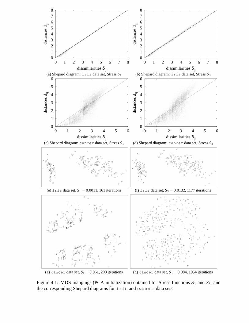


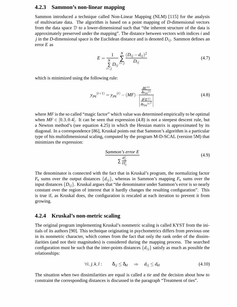
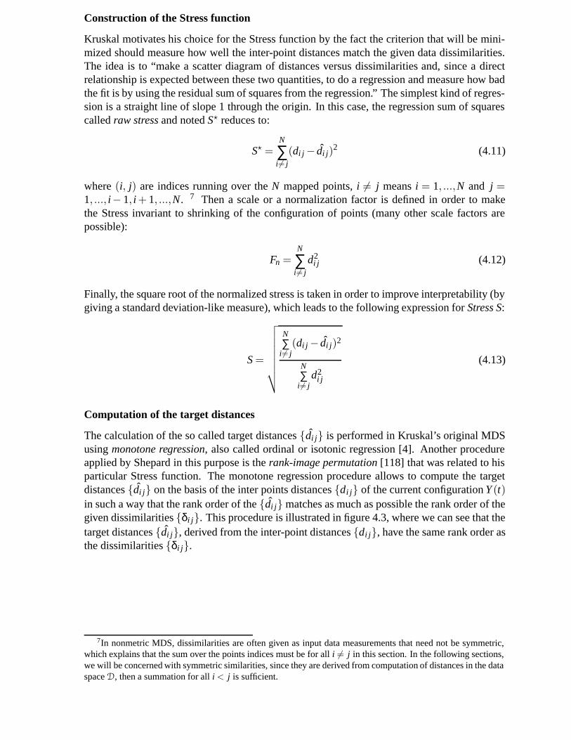


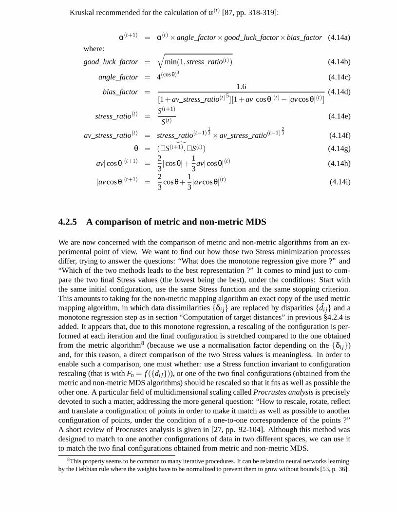


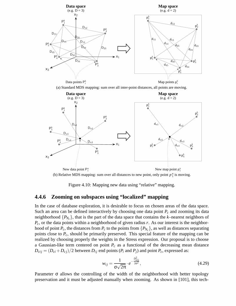


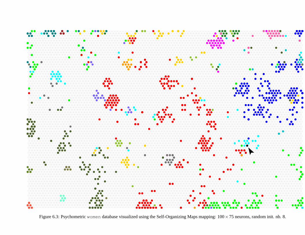
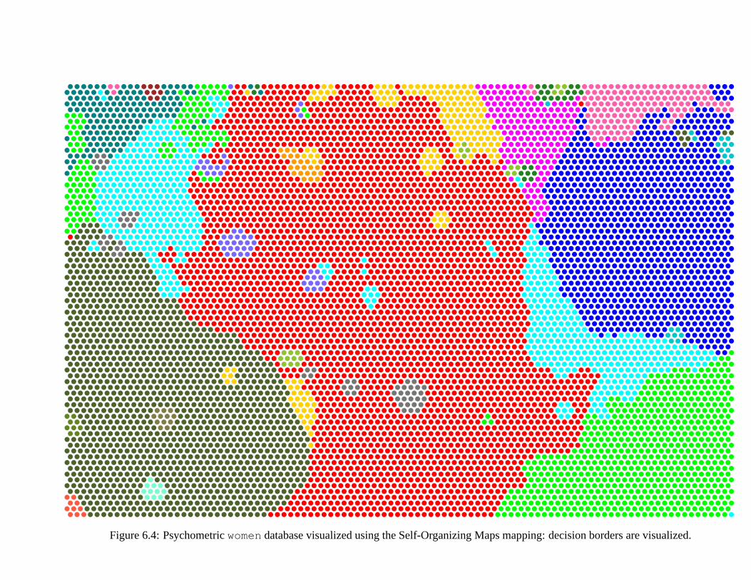


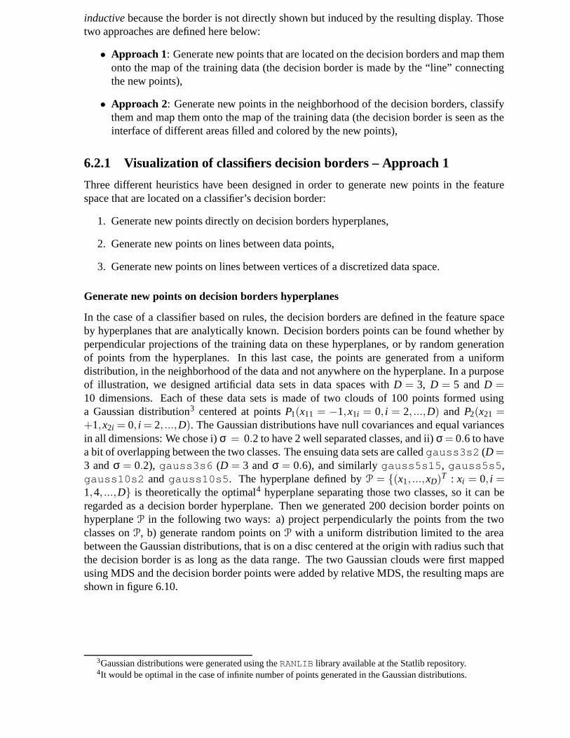


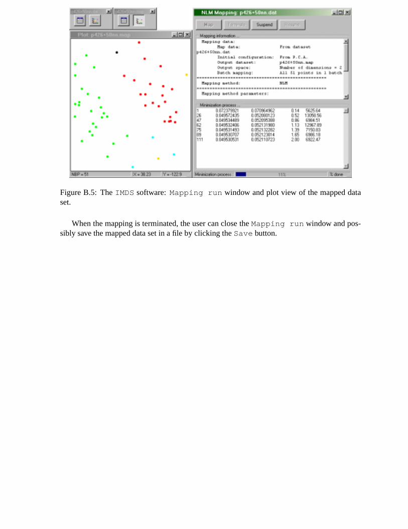


![[ KLIKNIJ I WPISZ NAZWĘ PRZEDMIOTU ] · A. Aho, J. E. Hopcroft, J. D. Ullman, Algorytmy i struktury danych, Helion, Gliwice, 2003. 3. J. Grebosz, Symfonia C++, Wydawnictwo Edition](https://static.documents.pub/doc/80x56/5b80ceb97f8b9ad9778e0933/-kliknij-i-wpisz-nazwe-przedmiotu-a-aho-j-e-hopcroft-j-d-ullman.jpg)

