1 MIXED FORMULATION USING IMPLICIT BOUNDARY FINITE ELEMENT METHOD By HAILONG CHEN A THESIS PRESENTED TO THE GRADUATE SCHOOL OF THE UNIVERSITY OF FLORIDA IN PARTIAL FULFILLMENT OF THE REQUIREMENTS FOR THE DEGREE OF MASTER OF SCIENCE UNIVERSITY OF FLORIDA 2012
Transcript
1
MIXED FORMULATION USING IMPLICIT BOUNDARY FINITE ELEMENT METHOD
By
HAILONG CHEN
A THESIS PRESENTED TO THE GRADUATE SCHOOL OF THE UNIVERSITY OF FLORIDA IN PARTIAL FULFILLMENT
OF THE REQUIREMENTS FOR THE DEGREE OF MASTER OF SCIENCE
B EQUILIBRIUM EQUATIONS OF 3D ELASTOSTATIC CASE .............................. 116
7
C DERIVATION OF SHEAR CORRECTION FACTOR ............................................ 118
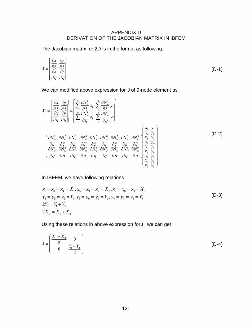
D DERIVATION OF THE JACOBIAN MATRIX IN IBFEM ........................................ 121
E FORMULATION OF MINDLIN PLATE ELEMENTS ............................................. 123
E.1 Element Q4D4 ................................................................................................ 123 E.2 Element Q5D6 ................................................................................................ 126 E.3 Element Q8D8 ................................................................................................ 128 E.4 Element Q9D12 .............................................................................................. 130 E.5 Element Q16D24 ............................................................................................ 132
LIST OF REFERENCES ............................................................................................. 136
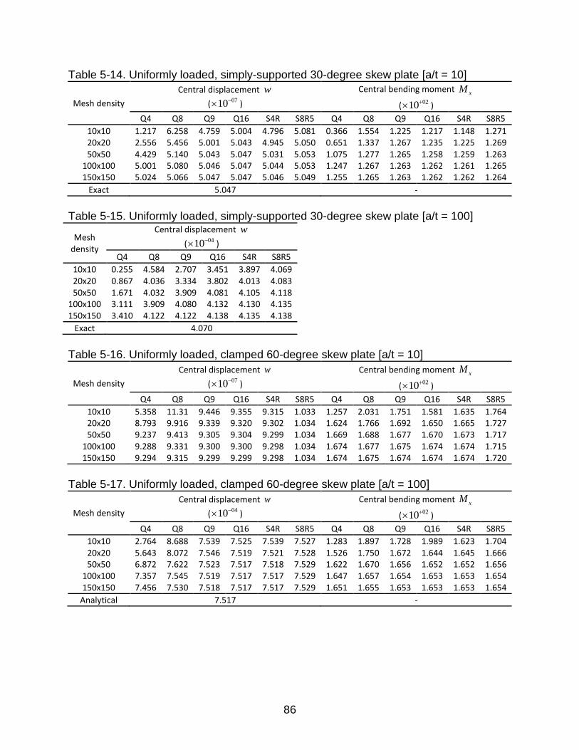
6-1 Transverse deflection of 60-degree skew plate with one edge clamped .......... 107
6-2 In plane displacement of 60-degree skew plate with one edge clamped .......... 107
9
6-3 Transverse deflection of square plate with one edge clamped ......................... 107
6-4 In plane displacement of square plate with one edge clamped ........................ 108
10
LIST OF FIGURES
Figure page 2-1 Conforming mesh in traditional FEM .................................................................. 24
2-2 Scattered nodes in meshless methods ............................................................... 24
2-3 Nonconforming structured mesh in IBFEM ......................................................... 24
2-4 Step function configuration in IBFEM ................................................................. 25
3-1 Geometry of the 2D bracket................................................................................ 40
3-2 Transverse displacement distribution after deformation (Q9M 130x80 mesh density) ............................................................................................................... 40
3-3 Maximum transverse displacement w.r.t Poisson’s ratio (Q4M) ......................... 40
3-4 Maximum transverse displacement w.r.t Poisson’s ratio (Q9M) ......................... 41
3-5 Geometry of 3D beam ........................................................................................ 41
3-6 Transverse displacement distribution after deformation (Hexa8M 65x10x10 mesh density) ..................................................................................................... 41
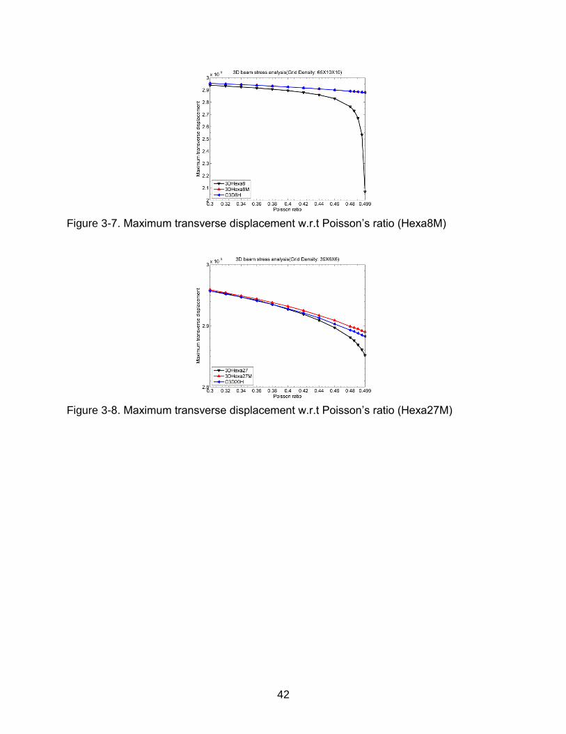
3-7 Maximum transverse displacement w.r.t Poisson’s ratio (Hexa8M) .................... 42
3-8 Maximum transverse displacement w.r.t Poisson’s ratio (Hexa27M) .................. 42
4-1 Configuration for CPT ......................................................................................... 62
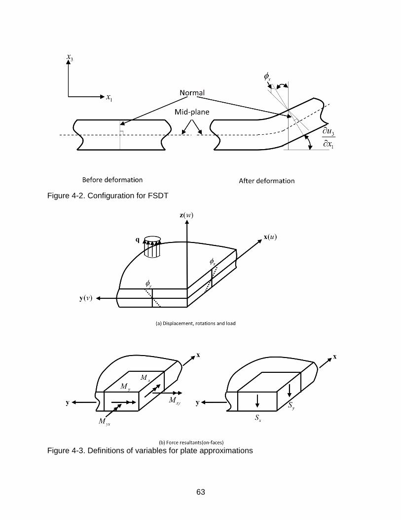
4-2 Configuration for FSDT ....................................................................................... 63
4-3 Definitions of variables for plate approximations ................................................ 63
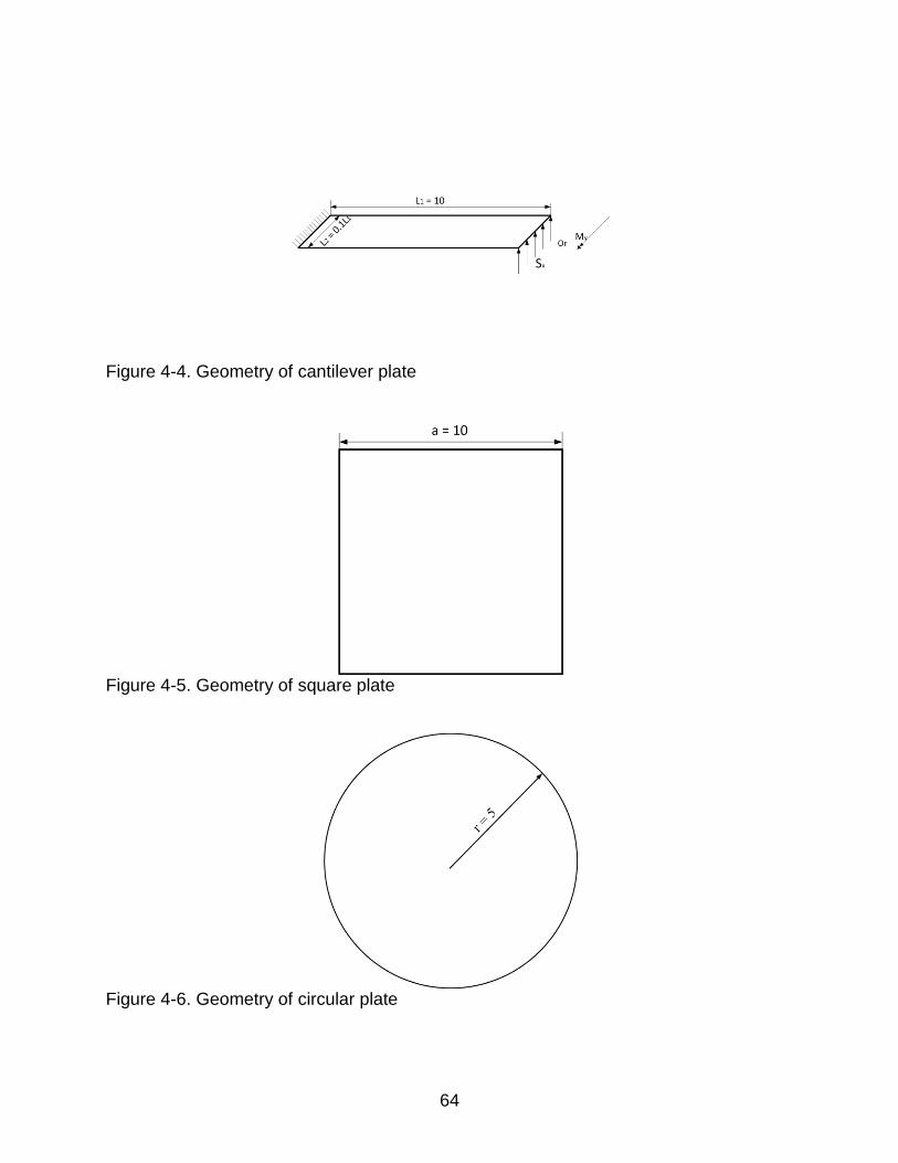
4-4 Geometry of cantilever plate ............................................................................... 64
4-5 Geometry of square plate ................................................................................... 64
4-6 Geometry of circular plate .................................................................................. 64
4-7 Geometry of 30-degree skew plate ..................................................................... 65
4-8 Geometry of 60-degree skew plate ..................................................................... 65
5-1 A typical background mesh using 20x2 Q4 element ........................................... 87
11
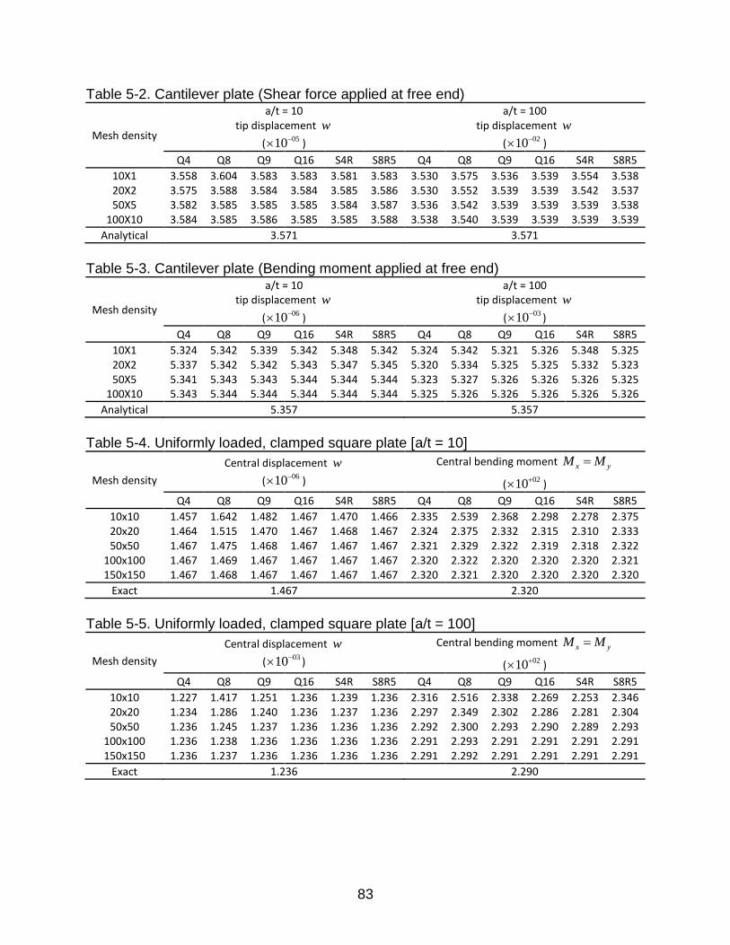
5-2 Distribution of transverse displacement after deformation for 100x10 Q4 element (L1/t = 100) ........................................................................................... 88
5-3 Convergence of total strain energy for cantilever when shear applied (L1/t = 10) ...................................................................................................................... 88
5-4 Convergence of total strain energy for cantilever when shear applied (L1/t = 100) .................................................................................................................... 88
5-5 Distribution of transverse displacement after deformation for 100x10 Q4 element (L1/t = 100) ........................................................................................... 89
5-6 Convergence of total strain energy for cantilever when bending moment applied (L1/t = 10) .............................................................................................. 89
5-7 Convergence of total strain energy for cantilever when bending moment applied (L1/t = 100) ............................................................................................ 89
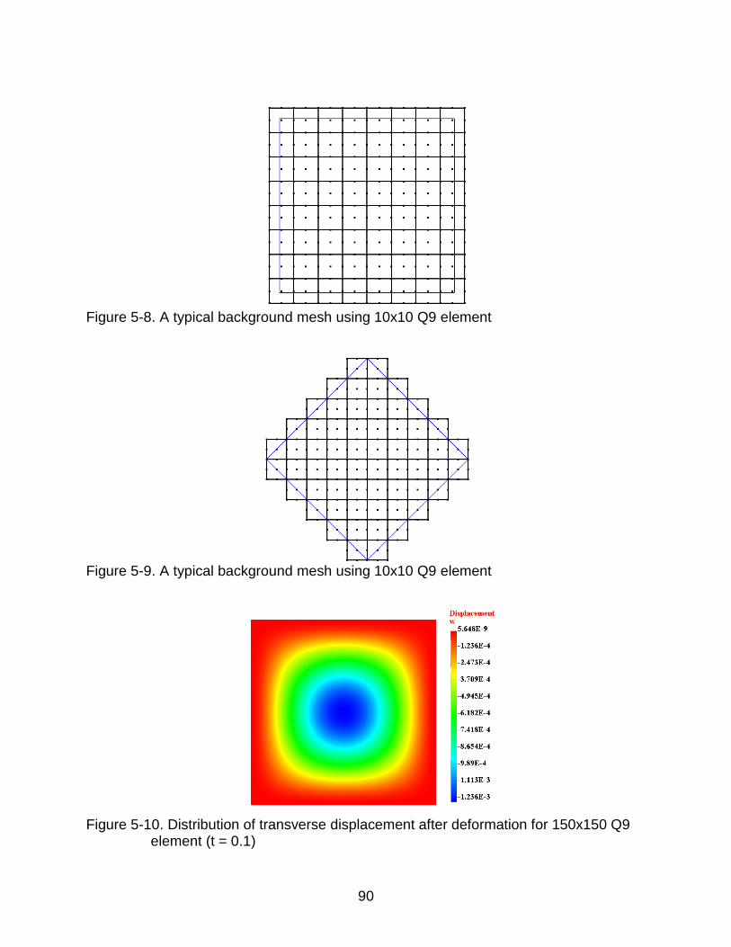
5-8 A typical background mesh using 10x10 Q9 element ......................................... 90
5-9 A typical background mesh using 10x10 Q9 element ......................................... 90
5-10 Distribution of transverse displacement after deformation for 150x150 Q9 element (t = 0.1) ................................................................................................. 90
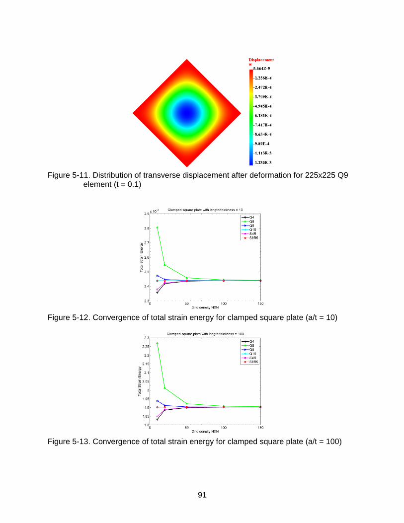
5-11 Distribution of transverse displacement after deformation for 225x225 Q9 element (t = 0.1) ................................................................................................. 91
5-12 Convergence of total strain energy for clamped square plate (a/t = 10) ............. 91
5-13 Convergence of total strain energy for clamped square plate (a/t = 100) ........... 91
5-14 Convergence of total strain energy for simply-supported square plate (a/t = 10) ...................................................................................................................... 92
5-15 Convergence of total strain energy for simply-supported square plate (a/t = 100) .................................................................................................................... 92
5-16 A typical background mesh using 10x10 Q4 element ......................................... 92
5-17 Distribution of transverse displacement after deformation for 150x150 Q4 element (t = 1) .................................................................................................... 93
5-18 Convergence of total strain energy for clamped circular plate (a/t = 10) ............ 93
5-19 Convergence of total strain energy for clamped circular plate (a/t = 100) .......... 93
5-20 Convergence of total strain energy for simply-supported circular plate (a/t = 10) ...................................................................................................................... 94
12
5-21 Convergence of total strain energy for simply-supported circular plate (a/t = 100) .................................................................................................................... 94
5-22 A typical background mesh using 10x10 Q8 element ......................................... 94
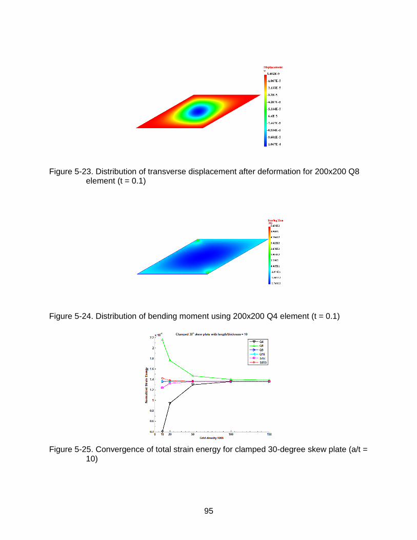
5-23 Distribution of transverse displacement after deformation for 200x200 Q8 element (t = 0.1) ................................................................................................. 95
5-24 Distribution of bending moment using 200x200 Q4 element (t = 0.1) ................. 95
5-25 Convergence of total strain energy for clamped 30-degree skew plate (a/t = 10) ...................................................................................................................... 95
5-26 Convergence of total strain energy for clamped 30-degree skew plate (a/t = 100) .................................................................................................................... 96
5-27 Convergence of total strain energy for simply-supported 30-degree skew plate (a/t = 10) .................................................................................................... 96
5-28 Convergence of total strain energy for simply-supported 30-degree skew plate (a/t = 100) .................................................................................................. 96
5-29 A typical background mesh using 10x10 Q16 element ....................................... 97
5-30 Distribution of transverse displacement after deformation for 200x200 Q9 element (t = 1) .................................................................................................... 97
5-31 Distribution of bending moment using 200x200 Q4 element (t = 0.1) ................. 97
5-32 Convergence of total strain energy for clamped 60-degree skew plate (a/t = 10) ...................................................................................................................... 98
5-33 Convergence of total strain energy for clamped 60-degree skew plate (a/t = 100) .................................................................................................................... 98
5-34 Convergence of total strain energy for simply-supported 60-degree skew plate (a/t = 10) .................................................................................................... 98
5-35 Convergence of total strain energy for simply-supported 60-degree skew plate (a/t = 100) .................................................................................................. 99
5-36 Geometry of flange plate .................................................................................... 99
5-37 A typical background mesh using 20x20 Q9 element ......................................... 99
5-38 Distribution of transverse displacement after deformation for 150x150 Q9 element (t = 0.1) ............................................................................................... 100
5-39 Convergence of total strain energy for arbitrary shape plate (a/t = 10) ............. 100
13
5-40 Convergence of total strain energy for arbitrary shape plate (a/t = 100) ........... 100
6-1 Convergence of total strain energy for 60-degree skew plate (a/t = 10) ........... 108
6-2 Convergence of total strain energy for 60-degree skew plate (a/t = 100) ......... 108
6-3 Distribution of transverse deflection after deformation for 60-degree skew plate using 150x150 Q4 element (t = 1)............................................................ 109
6-4 Geometry of the 60-degree skew plate ............................................................. 109
6-5 Convergence of total strain energy for square plate (a/t = 10) .......................... 109
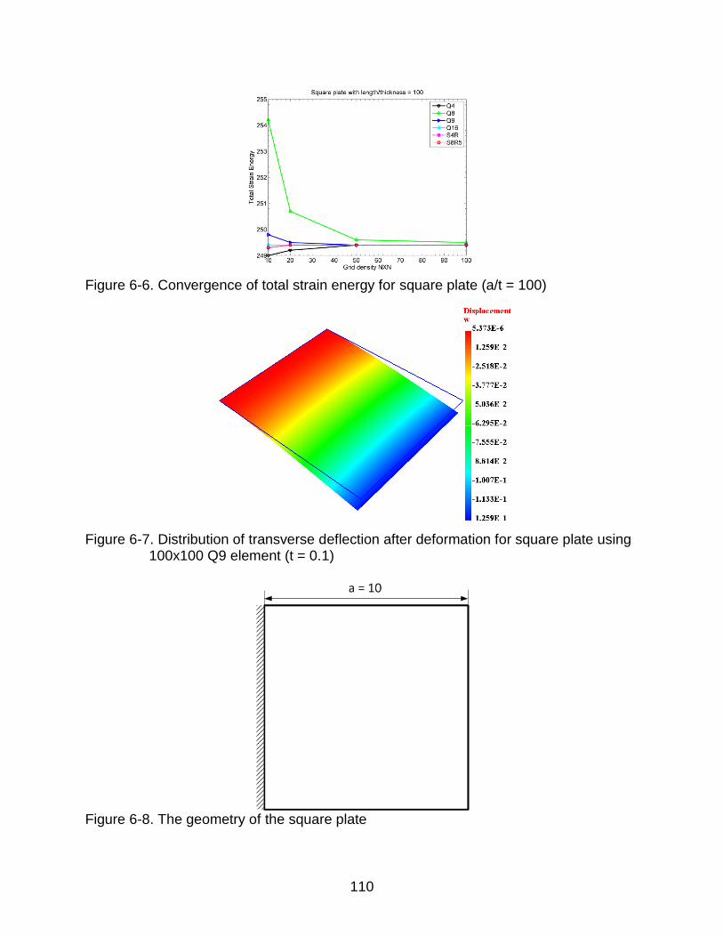
6-6 Convergence of total strain energy for square plate (a/t = 100) ........................ 110
6-7 Distribution of transverse deflection after deformation for square plate using 100x100 Q9 element (t = 0.1) ........................................................................... 110
6-8 The geometry of the square plate ..................................................................... 110
B-1 Stresses notations and directions ..................................................................... 116
C-1 Distribution of transverse shear stress through the thickness........................... 119
D-1 Global coordinate and Local coordinate in IBFEM ............................................ 122
E-1 Collocation constraints on a 4-node Lagrange element .................................... 123
E-2 Interpolation nodes for Q4D4 element .............................................................. 124
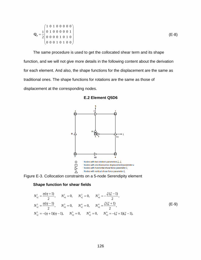
E-3 Collocation constraints on a 5-node Serendipity element ................................. 126
E-4 Interpolation nodes for Q5D6 element .............................................................. 127
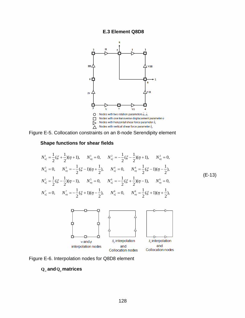
E-5 Collocation constraints on an 8-node Serendipity element ............................... 128
E-6 Interpolation nodes for Q8D8 element .............................................................. 128
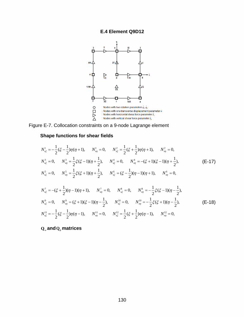
E-7 Collocation constraints on a 9-node Lagrange element .................................... 130
E-8 Interpolation nodes for Q9D12 element ............................................................ 131
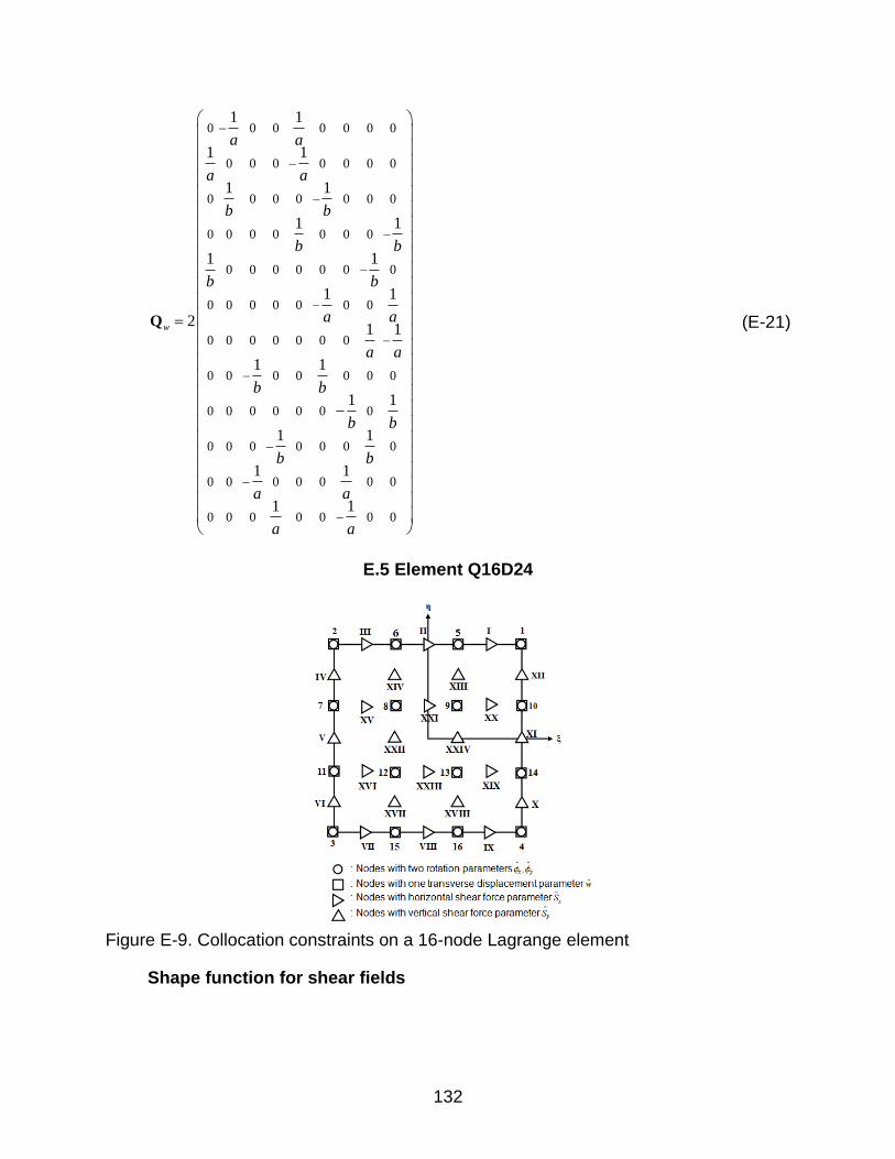
E-9 Collocation constraints on a 16-node Lagrange element .................................. 132
E-10 Interpolation nodes for Q16D24 element .......................................................... 135
CPE8H 8-node hybrid plane strain quadrilateral element, linear pressure
CPT Classical Plate Theory
EBC Essential Boundary Condition
FSDT First-Order Shear Deformable Theory
H27 27-node hexahedral element
H27M 27-node mixed hexahedral element
H8 8-node hexahedral element
H8M 8-node mixed hexahedral element
IBFEM Implicit Boundary Finite Element Method
LHS Left Hand Side
ODE Ordinary Differential Equation
Q4 4-node quadrilateral element
Q4M 4-node mixed quadrilateral element
Q8 8-node quadrilateral element
Q9 9-node quadrilateral element
Q9M 9-node mixed quadrilateral element
Q16 16-node quadrilateral element
RHS Right Hand Side
S4R 4-node doubly curved thin or thick shell element with reduced integration, hourglass control and finite membrane strains
S8R5 8-node doubly curved thin shell element with reduced integration using 5 degrees of freedom per node
15
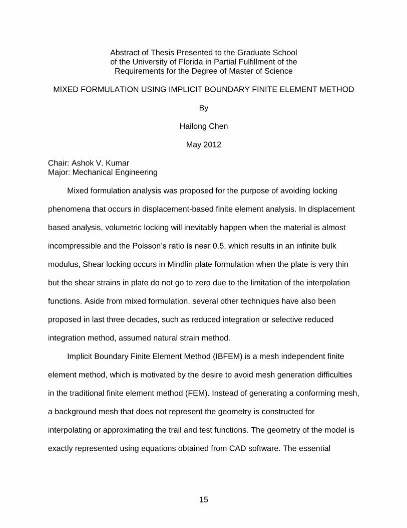
Abstract of Thesis Presented to the Graduate School of the University of Florida in Partial Fulfillment of the Requirements for the Degree of Master of Science
MIXED FORMULATION USING IMPLICIT BOUNDARY FINITE ELEMENT METHOD
By
Hailong Chen
May 2012
Chair: Ashok V. Kumar Major: Mechanical Engineering
Mixed formulation analysis was proposed for the purpose of avoiding locking
phenomena that occurs in displacement-based finite element analysis. In displacement
based analysis, volumetric locking will inevitably happen when the material is almost
incompressible and the Poisson’s ratio is near 0.5, which results in an infinite bulk
modulus, Shear locking occurs in Mindlin plate formulation when the plate is very thin
but the shear strains in plate do not go to zero due to the limitation of the interpolation
functions. Aside from mixed formulation, several other techniques have also been
proposed in last three decades, such as reduced integration or selective reduced
[20]. In this thesis, we will employ the mixed formulation to remove these locking
phenomena using Implicit Boundary Finite Element Method.
The main objectives of this thesis are
1. Extension of IBFEM to three-field mixed formulation for near incompressible media;
2. Extension of IBFEM to mixed formulation for Mindlin plates, pure bending;
3. Extension of IBFEM to 2D Mindlin shells, including both bending and in-plane stretching.
1.3 Outlines
The rest of this thesis is organized as follows:
In Chapter 1, a brief overview about FEM is presented, and the goals and
objectives of this thesis are clearly stated. In Chapter 2, we give some details and
reference to the meshless and mesh independent finite element methods. Two
20
challenges while using Implicit Boundary Finite Element Method are described and
scheme to solve these issues is presented. In Chapter 3, a three-field mixed formulation
for plane strain and 3D stress using IBFEM so as to remove the volumetric locking for
near incompressible media is derived in details. Two examples are used to test the
performance of this method. In Chapter 4, before proceeding to mixed formulation for
Mindlin plates, we review the two classical plate theories, Kirchhoff-Love plate theory
and Mindlin plate theory. The analytical or exact solution of several benchmark
problems, which used later to evaluate the performance of IBFEM, are given in Chapter
4 too. The two-field mixed formulation using Mindlin plate theory is detailed in Chapter
5. The focus is on the derivation of mixed form and imposing EBC using IBFEM. An
extension of Mindlin plate including both in plane stretching and bending is presented in
Chapter 6. Two examples have been used in Chapter 5, the same geometry but
different boundary conditions, are employed two test the performance of IBFEM for 2D
Mindlin shell case. The conclusion and future work is in Chapter 7. An appendix is also
included in order to give more details about some specific topics and also aimed to
make this thesis more self-contained.
21
CHAPTER 2 MESHLESS AND MESH INDEPENDENT METHOD
2.1 Traditional FEM
Finite Element Method ([1], [9], [21]) is a well established numerical technique and
is widely used in solving engineering problems such as stress analysis, heat transfer,
fluid flow and electromagnetics in academia as well as in industry.
According to Fish and Belytschko [6], the traditional Finite Element Method
consists of five procedures:
1. Preprocessing: subdividing the problem domain into finite elements and approximating the domain by these finite elements - mesh generation;
2. Element formulation: derivation of equations in the element level - discretization;
3. Element combination: obtaining the equation system for the approximated model from the equations of individual elements - assembly;
4. Solving the equations: using Gauss elimination, Cholesky decomposition or iterative schemes like Gauss-Siedel to solve the equation system;
5. Postprocessing: determining quantities of interest, such as displacement and force resultant, and visualizing the results for future evaluation - analysis.
Among above five procedures, mesh generation is the most challenge one, and
still most endeavors is spend on devising an effective automatic mesh generator for 3D
complex geometry, for which the generated mesh is unreliable nowadays. For finite
element analysis, the domain of interest is subdivided into small elements by mesh
generation techniques and the resulting element mesh approximates the geometry. A
typical mesh is shown in Figure 2-1. The mesh is also used to approximate the solution
by piece-wise interpolation within each element. In procedure 2, Galerkin’s approach is
employed to convert the strong from into weak form, namely, alleviate the interpolation
shape function degree requirement.
22
In order to avoid the problems associated with mesh generation, several
approaches have been proposed which falls into two categories:
1. Meshless methods;
2. Mesh independent methods.
Implicit Boundary Finite Element (IBFEM), [11]-[13], falls into the mesh
independent method category, which utilizes a structured background mesh only for the
purpose of interpolation. We will present some details about meshless and mesh
independent method in following two sections.
2.2 Meshless and Mesh Independent Method
The objective of meshless methods is to eliminate at least part of mesh generation
by constructing the approximation entirely in terms of nodes. A set of scattered nodes is
used to construct the trial and test function, see Figure 2-2. Several schemes are
developed to approximate these functions, such as moving least square method, kernel
method and partition of unity method, etc. [3].
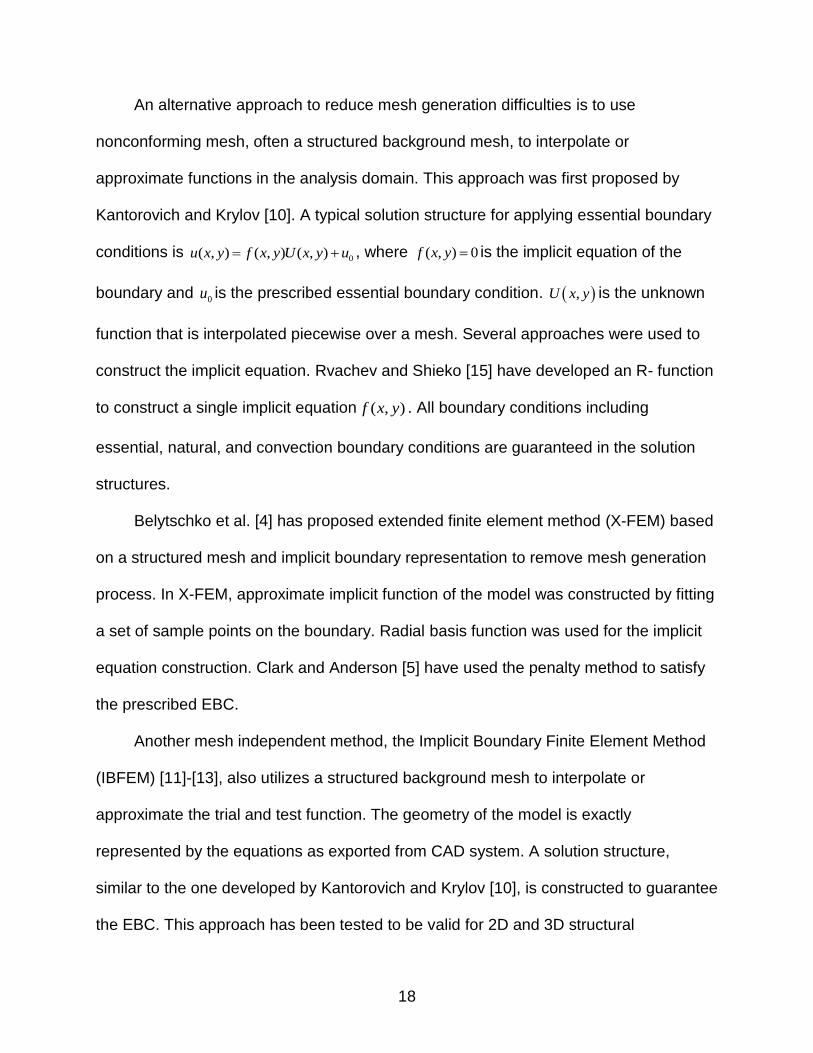
Mesh independent analysis is motivated by the desire to utilize accurate geometric
models presented by equations rather approximated by mesh while using a background
mesh solely for the purpose of piecewise approximation or interpolation of the trial and
test function. A solution structure is proposed by Kantorovich and Krylov [10],
0( , ) ( , ) ( , )u x y f x y U x y u , where ( , ) 0f x y is the implicit equation of the boundary and is
the essential boundary condition. ,U x y is the unknown function that interpolated
piecewise over a mesh. Rvachev and Shieko [15] have developed an R- function to
construct a single implicit equation to represent the entire boundary of a solid.
23
2.3 Implicit Boundary Finite Element Method
Comparing to traditional finite element method, Implicit Boundary Finite Element
Method (IBFEM) is a mesh independent finite element method, in which the geometry of
the model is exactly presented by the equations as exported from CAD system.
Although there is no geometry approximation in IBFEM, a background mesh (Figure 2-
3) is still employed but solely for the purpose of approximation or interpolation of the trial
and test function.
Contrary to the R-function technique used in Rvachev and Shieko [15], an
approximate step function was used in IBFEM to construct the implicit equation of the
interested domain. The solution structure used in IBFEM is
0( ) ( ) ( )u H U u x x x (2-1)
where ( , )H x y is the step function. A typical approximate step function being used
in IBFEM is
0 0
(2 ), 0
1
iH
(2-2)
where i can be 1,2,3 , is the distance between point to the boundary lines in the
normal direction, and is the transition width, see Figure 2-4.
24
Figure 2-1. Conforming mesh in traditional FEM
Figure 2-2. Scattered nodes in meshless methods
Figure 2-3. Nonconforming structured mesh in IBFEM
25
Figure 2-4. Step function configuration in IBFEM
26
CHAPTER 3 MIXED FORMULATION FOR NEARLY INCOMPRESSIBLE MEDIA
3.1 Overview
It has been frequently noted that in certain constitutive laws, such as those of
viscoelasticity and associative plasticity, the material behaves in a nearly
incompressible manner. The incompressibility of these media, at certain critical stage,
e.g., metals at the range of plastic deformations (yielding), results in a locking
phenomenon, named volumetric locking or Poisson locking. This phenomenon results
from the fact that when the material is near incompressible status, the Poisson’s ratio, v ,
tends to 0.5, which makes the bulk modulus / (3 6 )E v tend towards infinity and
hence result in a ill-conditioned stiffness matrix in the finite element model.
Several approaches have been proposed in last three decades to reduce or
alleviate volumetric locking occurrence. Reduced or selective reduced integration
technique was the first successful irreducible form of solutions for volumetric locking
problems, although in the beginning not directed specially towards volumetric locking.
Later, other formulations succeeded in using augmented functional, when compared to
that obtained from displacement-based approaches, incorporating additional fields into
the formulation and leading to the onset of general mixed methods. In the 1990s, the
enhanced strain method was also applied to alleviate this locking phenomenon.
Generally, there are two choices of mixed formulation on additional fields,
displacement u and mean stress p , which named two-field formulation, and
displacement u , mean stress p and volume changev , termed three-field formulation
([1], [9], [21]). Which of these should be employed may depend on the form of the
constitutive equation used. For situations where changes in volume affect only the
27
pressure the two-field form can be easily used. However, for problems in which the
response may become coupled between the deviatoric and mean components of stress
and strain the three-field formulation leads to much simpler forms from which to develop
a finite element model. In this thesis, we will only focus on the later formulation, three-
field mixed formulation.
The layout of Chapter 3 is as follows:
In section 3.2, we derive the general mixed formulation, and the resultant
equations using three-field formulation;
In section 3.3 and 3.4, we specify our discussion to 2D plan strain and 3D stress
respectively. A further modification of the mixed forms for 4-node and 9-node Lagrange
elements in 2D case and 8-node and 27-node hexahedron elements for 3D case;
In section 3.5, we employ some benchmark problems to test the performance of
elements developed in IBFEM. The conclusion of Chapter 3 is made in section 3.6.
3.2 Mixed Formulation
As mentioned in the introduction of Chapter 3, a three-field mixed formulation is
adopted in this section to develop some valuable elements both for 2D plane strain and
3D stress using IBFEM. In this section, we will develop the general mixed form for both
cases.
3.2.1 Matrix Decomposition
Generally, in most cases, the strain and stress matrices can be split into the
deviator (isochoric) and mean parts. Since the separation slightly differs for 2D and 3D.
Here, we utilize 3D case for illustration. That for 2D will be presented in section 3.3.
Accordingly, the mean stress, pressure part, can be expressed as
28
11 22 33( )1 1
3 3 iip (3-1)
We use sum notation here. And 1,2,3i .
And the deviatoric part can be defined as
( )ij ij ijdp (3-2)
where ij is the Kronecker delta function, which when i j is one and else zero for
all , 1,2,3i j .
Similarly, the mean strain, volume change, can be defined as
11 22 33)(v ii (3-3)
and the deviatoric strain as
1( )
3 vij ij ijd (3-4)
Have above definitions for mean part and deviatoric part of stress and strain, the
strain and stress may now be expressed in a mixed form as
Strain 1
( )3 vd
ε I u m (3-5)
Stress dp σ I σ m (3-6)
where the mean matrix operator
(1 1 1 0 0 0)Tm (3-7)
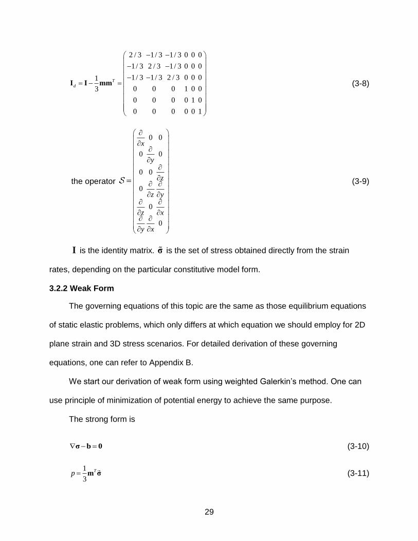
and deviatoric matrix operator
29
2 / 3 1/ 3 1/ 3 0 0 0
1/ 3 2 / 3 1/ 3 0 0 0
1/ 3 1/ 3 2 / 3 0 0 01
0 0 0 1 0 03
0 0 0 0 1 0
0 0 0 0 0 1
T
d
I I mm (3-8)
the operator
0 0
0 0
0 0
0
0
0
x
y
z
z y
z x
y x
(3-9)
I is the identity matrix. σ is the set of stress obtained directly from the strain
rates, depending on the particular constitutive model form.
3.2.2 Weak Form
The governing equations of this topic are the same as those equilibrium equations
of static elastic problems, which only differs at which equation we should employ for 2D
plane strain and 3D stress scenarios. For detailed derivation of these governing
equations, one can refer to Appendix B.
We start our derivation of weak form using weighted Galerkin’s method. One can
use principle of minimization of potential energy to achieve the same purpose.
The strong form is
σ b 0 (3-10)
1
3
Tp m σ (3-11)
30
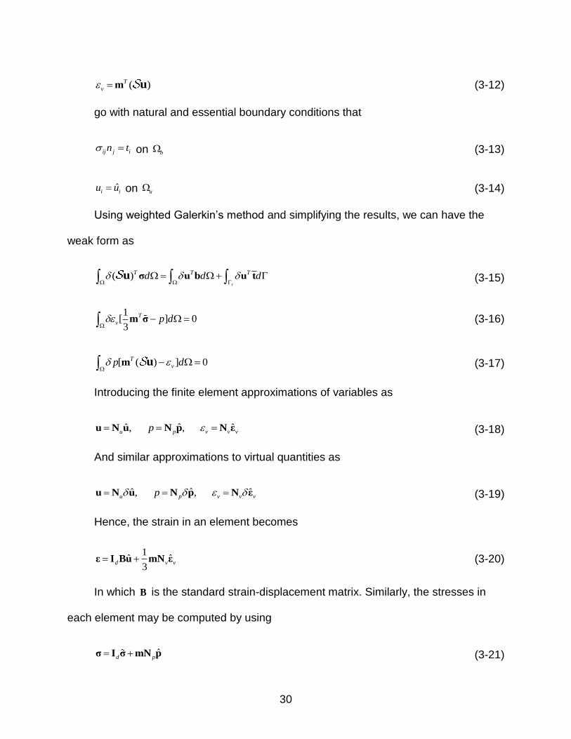
( )T
v m u (3-12)
go with natural and essential boundary conditions that
ij j in t on b (3-13)
ˆi iu u on u (3-14)
Using weighted Galerkin’s method and simplifying the results, we can have the
weak form as
( )t
T T Td d d
σ u b u tu (3-15)
1[ ] 03
T
v p d
m σ (3-16)
[ ( ) ] 0T
vp d
m u (3-17)
Introducing the finite element approximations of variables as
ˆˆ ˆ, ,u p v v vp u N u N p N ε (3-18)
And similar approximations to virtual quantities as
ˆˆ ˆ, ,u p v v vp u N u N p N ε (3-19)
Hence, the strain in an element becomes
1ˆ ˆ
3d v v ε I Bu mN ε (3-20)
In which B is the standard strain-displacement matrix. Similarly, the stresses in
each element may be computed by using
ˆd p σ I σ mN p (3-21)
31
Since strain εand stressσ are the element variables, we will keep it as constant
while constructing the weak form system.
Substitute Equations 3-18 and 3-19 into the weak form Equations 3-15 to 3-17, we
have
For Equation 3-15:
(
ˆ ˆ( ( ) ( )
)
ˆ )
t
t
t
T T T
T T T
u u u
T T T
u u
d d d
d d d
d d d
σ u b u t
N σ N u b N u t
B σ N b N t
u
u (3-22)
For Equation 3-16:
1ˆˆ [ ] 0
3
1ˆ( ) 0
3
T T
v v p
T T T
v v p
d
d d
N ε m σ N p
N m σ N N p
(3-23)
For Equation 3-17:
ˆ ˆ[ ( ) ] 0
ˆ( ) ( ) 0
ˆ
ˆ
T T
p u v v
T T T
p p v v
d
d d
N p m N N ε
N m B N N ε
u
u (3-24)
Writing Equations 3-22 to 3-24 in matrix form, the finite element equation system
becomes
ˆ ˆ
ˆ
T
vp v pu
p vp
P f
K ε K u 0
P K p 0 (3-25)
Where
T d
P B σ , 1
3
T T
p v d
P N m σ , T
vp v pd
K N N , T T
pu p d
K N m B
t
T T
u ud d
f N b N t
32
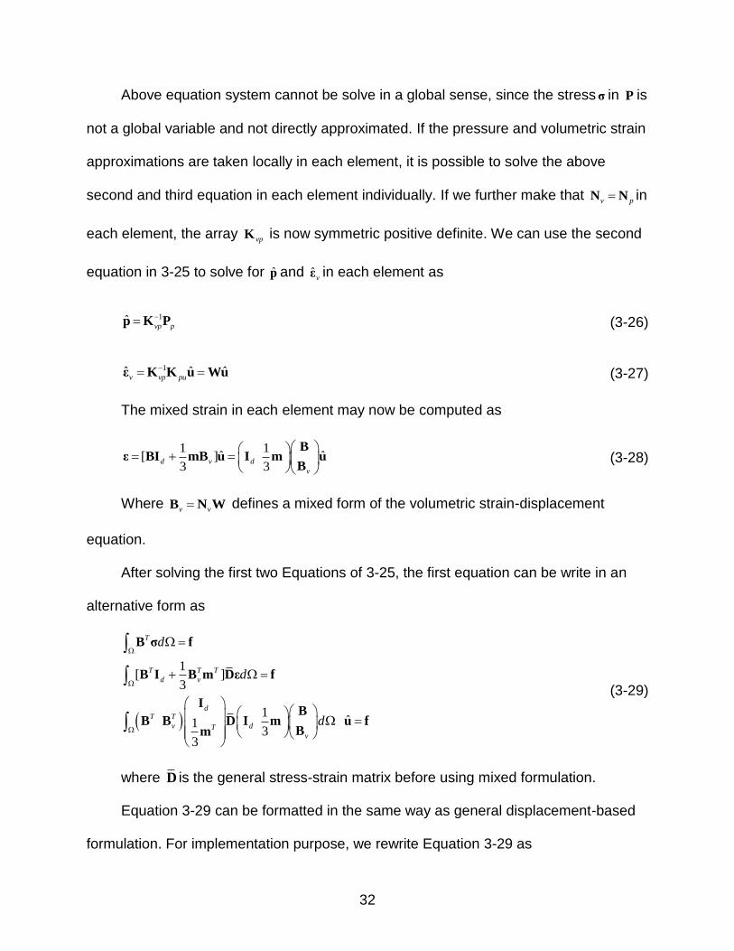
Above equation system cannot be solve in a global sense, since the stressσ in P is
not a global variable and not directly approximated. If the pressure and volumetric strain
approximations are taken locally in each element, it is possible to solve the above
second and third equation in each element individually. If we further make that v pN N in
each element, the array vpK is now symmetric positive definite. We can use the second
equation in 3-25 to solve for p and ˆvε in each element as
1ˆvp p
p K P (3-26)
1ˆ ˆ ˆv vp pu
ε K K u Wu (3-27)
The mixed strain in each element may now be computed as
1 1ˆ ˆ[ ]
3 3d v d
v
Bε BI mB u I m u
B (3-28)
Where v vB N W defines a mixed form of the volumetric strain-displacement
equation.
After solving the first two Equations of 3-25, the first equation can be write in an
alternative form as
1[ ]
3
1ˆ1
33
T
T T T
d v
dT T
v dTv
d
d
d
B σ f
B I B m Dε f
IB
B B D I m u fBm
(3-29)
where D is the general stress-strain matrix before using mixed formulation.
Equation 3-29 can be formatted in the same way as general displacement-based
formulation. For implementation purpose, we rewrite Equation 3-29 as
33
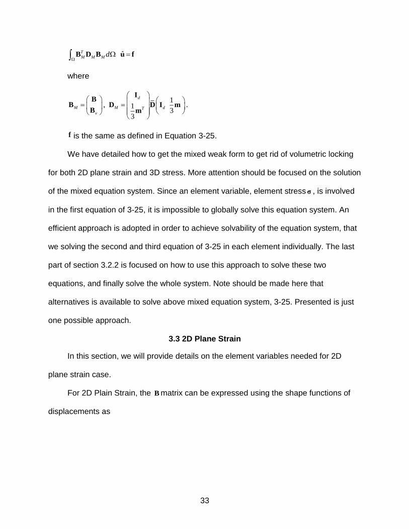
ˆT
M M M d
B D B u f
where
M
v
BB
B,
11
33
d
M dT
I
D D I mm
.
f is the same as defined in Equation 3-25.
We have detailed how to get the mixed weak form to get rid of volumetric locking
for both 2D plane strain and 3D stress. More attention should be focused on the solution
of the mixed equation system. Since an element variable, element stress σ , is involved
in the first equation of 3-25, it is impossible to globally solve this equation system. An
efficient approach is adopted in order to achieve solvability of the equation system, that
we solving the second and third equation of 3-25 in each element individually. The last
part of section 3.2.2 is focused on how to use this approach to solve these two
equations, and finally solve the whole system. Note should be made here that
alternatives is available to solve above mixed equation system, 3-25. Presented is just
one possible approach.
3.3 2D Plane Strain
In this section, we will provide details on the element variables needed for 2D
plane strain case.
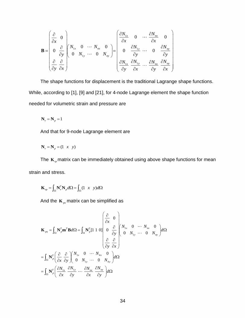
For 2D Plain Strain, the B matrix can be expressed using the shape functions of
displacements as
34
1
1 1
1
11
0 00
0 00 0 0
0 0
x nx
x nx y ny
y ny
y nyx nx
N N
x xxN N N N
N Ny y y
N NN N
y x y x y x
B
The shape functions for displacement is the traditional Lagrange shape functions.
While, according to [1], [9] and [21], for 4-node Lagrange element the shape function
needed for volumetric strain and pressure are
1v p N N
And that for 9-node Lagrange element are
(1 )v p x y N N
The vpK matrix can be immediately obtained using above shape functions for mean
strain and stress.
(1 )T
vp v pd x y d
K N N
And the puK matrix can be simplified as
1
1
1 4
1 4
11
0
0 0[1 1 0] 0
0 0
0 0
0 0
x nxT T T
pu p p
y ny
x xT
p
y y
y nyT x nxp
xN N
d dN Ny
y x
N Nd
N Nx y
N NN Nd
x y x y
K N m B N
N
N
35
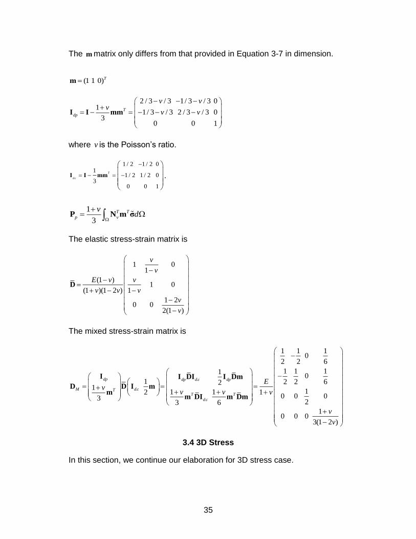
The m matrix only differs from that provided in Equation 3-7 in dimension.
(1 1 0)Tm
2 / 3 / 3 1/ 3 / 3 01
1/ 3 / 3 2 / 3 / 3 03
0 0 1
T
dp
v vv
v v
I I mm
where v is the Poisson’s ratio.
1 / 2 1 / 2 01
1 / 2 1 / 2 03
0 0 1
T
d
I I mm .
1
3
T T
p v
vd
P N m σ
The elastic stress-strain matrix is
1 01
(1 )1 0
(1 )(1 2 ) 1
1 20 0
2(1 )
v
v
E v v
v v v
v
v
D
The mixed stress-strain matrix is
1 1 10
2 2 6
1 1 110
1 2 2 621
11 12 10 0 03
23 6
10 0 0
3(1 2 )
dp dp d dp
M dTT T
d
Ev
v v v
v
v
I I DI I Dm
D D I mm
m DI m Dm
3.4 3D Stress
In this section, we continue our elaboration for 3D stress case.
36
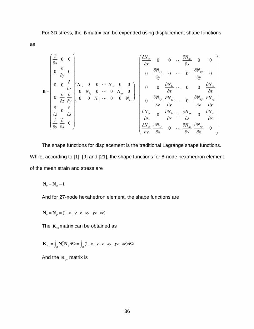
For 3D stress, the B matrix can be expended using displacement shape functions
as
1
1
1
0 0
0 0
0 0 0 00 0
0 0 0 0
0 0 0 0 0
0
0
x nx
y ny
z nz
x
y
N Nz
N N
N Nz y
z x
y x
B
1
1
1
1 1
1 1
11
0 0 0 0
0 0 0 0
0 0 0 0
0 0
0 0
0 0
x nx
y ny
nzz
y ny nzz
x nx nzz
y nyx nx
N N
x x
N N
y y
NN
z z
N N NN
z y z y
N N NN
z x z x
N NN N
y x y x
The shape functions for displacement is the traditional Lagrange shape functions.
While, according to [1], [9] and [21], the shape functions for 8-node hexahedron element
of the mean strain and stress are
1v p N N
And for 27-node hexahedron element, the shape functions are
(1 )v p x y z xy yz xz N N
The vpK matrix can be obtained as
(1 )T
vp v pd x y z xy yz xz d
K N N
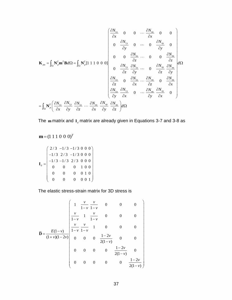
And the puK matrix is
37
1
1
1
1 1
1 1
11
0 0 0 0
0 0 0 0
0 0 0 0
[1 1 1 0 0 0]
0 0
0 0
0 0
x nx
y ny
nzz
T T T
pu p py ny nzz
x nx nzz
y nyx nx
N N
x x
N N
y y
NN
z zd d
N N NN
z y z y
N N NN
z x z x
N NN N
y x y x
K N m B N
N11 1y nyT x nx nzz
p
N NN N NNd
x y z x y z
The m matrix and dI matrix are already given in Equations 3-7 and 3-8 as
(1 1 1 0 0 0)Tm
2 / 3 1/ 3 1/ 3 0 0 0
1/ 3 2 / 3 1/ 3 0 0 0
1/ 3 1/ 3 2 / 3 0 0 0
0 0 0 1 0 0
0 0 0 0 1 0
0 0 0 0 0 1
d
I
The elastic stress-strain matrix for 3D stress is
1 0 0 01 1
1 0 0 01 1
1 0 0 01 1(1 )
1 2(1 )(1 2 ) 0 0 0 0 02(1 )
1 20 0 0 0 0
2(1 )
1 20 0 0 0 0
2(1 )
v v
v v
v v
v v
v v
v vE vvv vv
v
v
v
v
D
38
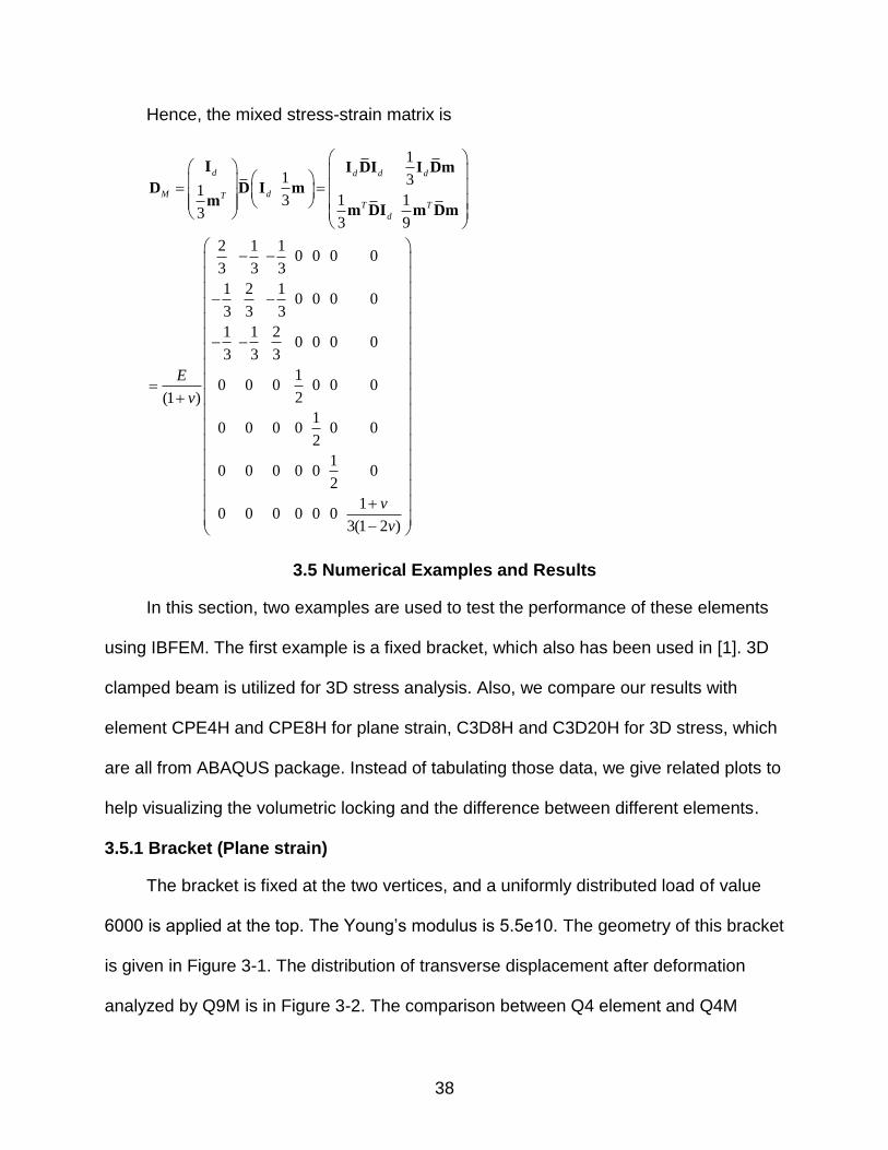
Hence, the mixed stress-strain matrix is
1
1 31
1 133
3 9
2 1 10 0 0 0
3 3 3
1 2 10 0 0 0
3 3 3
1 1 20 0 0 0
3 3 3
10 0 0 0 0 0
2(1 )
10 0 0 0 0 0
2
10 0 0 0 0 0
2
10 0 0 0 0 0
3(1 2 )
d d d d
M dTT T
d
E
v
v
v
I I DI I Dm
D D I mm
m DI m Dm
3.5 Numerical Examples and Results
In this section, two examples are used to test the performance of these elements
using IBFEM. The first example is a fixed bracket, which also has been used in [1]. 3D
clamped beam is utilized for 3D stress analysis. Also, we compare our results with
element CPE4H and CPE8H for plane strain, C3D8H and C3D20H for 3D stress, which
are all from ABAQUS package. Instead of tabulating those data, we give related plots to
help visualizing the volumetric locking and the difference between different elements.
3.5.1 Bracket (Plane strain)
The bracket is fixed at the two vertices, and a uniformly distributed load of value
6000 is applied at the top. The Young’s modulus is 5.5e10. The geometry of this bracket
is given in Figure 3-1. The distribution of transverse displacement after deformation
analyzed by Q9M is in Figure 3-2. The comparison between Q4 element and Q4M
39
element, Q9 element and Q9M element is plotted in Figure 3-3 and Figure 3-4,
respectively. From Figures 3-3 and 3-4, volumetric locking is very severe in Q4 element,
while with the increase of degree of shape function, using Q9 element, this
phenomenon can be better improved, but still cannot be avoided. See Figure 3-4.
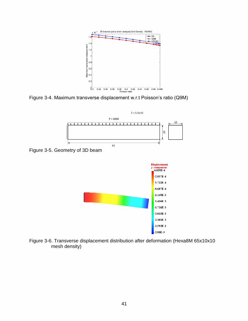
3.5.2 Beam (3D stress)
A beam clamped at the left end is loaded with a distributed load of 6000 at the top
surface. The Young’s modulus is 5.5e10. The geometry of this beam is shown in Figure
3-5. The deformed shape of the beam with transverse displacement distribution is given
in Figure 3-6. The comparison between different elements also given in this example,
Figure 3-7 and Figure 3-8. From Figures 3-7 and 3-8, volumetric locking is also drastic
in H8 element, while with the increase of degree of shape function, using H27 element,
this phenomenon is better improved, but still cannot avoid. See Figure 3-8.
3.6 Concluding Remarks
A three-field mixed formulation scheme has been adopted in Chapter 3 to remove
or alleviate the volumetric locking in 2D plane strain and 3D stress. The detailed
derivation of such formulation is presented in section 3.1, 3.2 and 3.3. Two examples
are employed to test the validity of the developed elements using IBFEM. The
comparison between displacement based formulation and the three-field mixed
formulation is also presented in these two examples. Elements from Abaqus package
are also used in the comparison. From the results and plots given, it’s obviously that
these IBFEM elements can better remove or alleviate volumetric locking phenomenon in
both 2D plane strain and 3D stress, and performs the same, if not better than, as the
Abaqus elements.
40
Figure 3-1. Geometry of the 2D bracket
Figure 3-2. Transverse displacement distribution after deformation (Q9M 130x80 mesh
density)
Figure 3-3. Maximum transverse displacement w.r.t Poisson’s ratio (Q4M)
41
Figure 3-4. Maximum transverse displacement w.r.t Poisson’s ratio (Q9M)
Figure 3-5. Geometry of 3D beam
Figure 3-6. Transverse displacement distribution after deformation (Hexa8M 65x10x10
mesh density)
42
Figure 3-7. Maximum transverse displacement w.r.t Poisson’s ratio (Hexa8M)
Figure 3-8. Maximum transverse displacement w.r.t Poisson’s ratio (Hexa27M)
43
CHAPTER 4 CLASSICAL PLATE THEORIES
4.1 Overview
The plate element has attracted considerable amount of attentions due to its great
application in engineering field. Among numerous plate theories that have been
developed since the late nineteenth century, the first widely accepted and used in
engineering was proposed by Kirchhoff and developed by Love, named Kirchhoff-Love
(KL) plate theory, which is an extension of Euler-Bernoulli beam theory. In KL plate
theory, it’s assumed that the transverse normals remain straight and perpendicular to
the mid-plane of the plate before and after deformation, and the strain in the thickness
direction is negligible. In other word, the strains , ,xz yz zz are negligibly zero in KL plate
theory. These assumptions render KL plate theory only applicable for thin structures
and C1 continuity is required for shape functions. Mindlin and Reissner have relaxed
Kirchhoff assumption to include the shear flexibility in the plate theory, which called
Mindlin-Reissner (MR) plate theory or First-order shear deformation theory. In MR plate
theory, the normal not necessary perpendicular to the mid-plane and the transverse
shear strains should be taken into consideration. Inclusion of the shear flexibility in the
MR plate theory makes it comparatively suitable for moderately thick plates and only C0
continuity is required. However, MR plate elements exhibit a phenomenon termed shear
locking when the thickness of the plate tends to zero.
Over last three decades, extensive efforts have been spent to device an effective
finite element scheme to overcome shear locking phenomenon for MR plate element. A
lot of finite element techniques have been developed, including but not limited to:
Reduced Integration or Selective Reduced Integration method, Mixed/Hybrid method,
Figure E-10. Interpolation nodes for Q16D24 element
136
LIST OF REFERENCES
[1] Bathe, K.J. (1996). Finite Element Procedures, 2nd ed., Prentice-Hall, New Jersey.
[2] Bathe, K.J., Dvorkin, E.N. (1985). A four-node plate bending element based on Mindlin/Reissner plate theory and a mixed interpolation. International Journal of Numerical Methods in Engineering, 21(2), 367-383.
[3] Belytschko, T., Krongauz, Y., Organ, D., Fleming, M., Krysl, P. (1996). Meshless Methods: An Overview and Recent Developments. Computer Methods in Applied Mechanics and Engineering, 139, 3-47.
[4] Belytschko, T., Parimi, C., Moes, N., Usui, S., Sukumar, N. (2003). Structured extended finite element methods for solids defined by implicit surfaces. International Journal for Numerical Methods in Engineering, 56(4), 609-635.
[5] Clark, B.W., Anderson, D.C. (2002). Finite Element Analysis in 3D Using Penalty Boundary Method. Proceedings of Design Engineering Technical Conferences, Montreal, Canada.
[6] Fish, J., Belytschko, T. (2007). A first course in finite elements, John Wiley and Sons.
[7] Hinton, E., Huang, H.C. (1986). A family of quadrilateral Mindlin plate elements with substitute shear strain fields. Computers and Structures, 23 (3), 409-431.
[8] Hrabok, M.M., Hrudey, T.M. (1984). A review and catalogue of plate bending finite elements. Computers and Structures, 19(3), 479-495.
[9] Hughes, T.J.R. (2000). The Finite Element Method: Linear Static and Dynamic Finite Element Analysis, 2nd edition. Dover Editions, New Jersey.
[10] Kantorovich, L.W., Krylov, W.I. (1956). Näherungsmethoden der Höheren Analysis. VEB Deutscher Verlag der Wissenschaften, Berlin.
[11] Kumar, A.V., Burla, R., Padmanabhan, S., Gu, L. (2008). Finite element analysis using nonconforming mesh. Journal of Computing and Information Science in Engineering, 8, 031005-1.
[12] Kumar, A.V., Lee, J. (2003). Step function representation of solid models and application to mesh free engineering analysis, Journal of Mechanical Design. Transactions of the ASME, 128(1), 46-56.
[13] Kumar, A.V., Padmanabhan, S., Burla, R. (2008). Implicit boundary method for finite element analysis using non-conforming mesh or mesh. International Journal for Numerical Methods in Engineering, 74 (9), 1421-1447.
[15] Rvachev, V.L., Shieko, T.I. (1995). R-functions in Boundary Value Problems in Mechanics. Applied Mechanics Review, 48, 151-188.
[16] Sengupta, D. (1995). Performance study of a simple finite element in the analysis of skew rhombic plates. Computers and Structures, 54 (6), 1173-1182.
[17] Taylor, R.L., Govindjee, S. (2004. )Solution of clamped rectangular problems. Communications in Numerical Methods in Engineering. 20, 757-765.
[18] Timoshenko, S., Woinowsky-Kreiger, S. (1987). Theory of Plates and Shells, second edition. McGraw-Hill, New York.
[19] Wang, C.M., Reddy, J.N., Lee, K.H. (2000). Shear Deformable Beams and Plates: Relationships with Classical Solutions. Elsevier, Oxford.
[20] Yang, T.Y., Saigal, S., Masud, A., Kapania, R.K. (2000). A survey of recent shell finite elements. International Journal for Numerical Methods in Engineering, 47, 101-127.
[21] Zienkiewicz, O.C., Taylor, R.L., Zhu, J.Z. (2005). The Finite Element Method for Solid and Structural Mechanics, sixth edition. Butterworth-Heinemann.
[22] Zienkiewicz, O.C., Xu, Z., Zeng, L.F., Samuelson, Wilbert, N.E. (1993). Linked interpolation for Reissner – Mindlin plate elements: Part I - A simple quadrilateral. International Journal for numerical Methods in Engineering, 36, 3043 – 3056.
138
BIOGRAPHICAL SKETCH
Hailong Chen was born and brought up in Jiangxi, China. He graduated with a
Bachelor of Science in engineering degree in mechanical engineering from Shanghai
Normal University, Shanghai, China in June 2010 with honors. After graduation, he
directly enrolled in the master’s program in Mechanical and Aerospace Engineering at
the University of Florida in fall 2010 with Achievement Award for New Engineering
Graduate Students. In 2011, he and Xiao Zhou got married in China. His area of interest
includes application of FEM in plates and shells, numerical methods and uncertainty