By - KU ScholarWorks

AN UNCONDITIONALLY STABLE METHOD FOR NUMERICALLY SOLVING SOLAR

SAIL SPACECRAFT EQUATIONS OF MOTION

By

Alex Karwas

Submitted to the graduate degree program in Aerospace Engineering and the Graduate Faculty of

the University of Kansas in partial fulfillment of the requirements for the degree of Doctor of

Philosophy.

________________________________

Chairperson Ray Taghavi, PhD

________________________________

Saeed Farokhi, PhD

________________________________

Shawn Keshmiri, PhD

________________________________

Zhongquan Charlie Zheng, PhD

________________________________

Bedru Yimer, PhD

Date Defended: March 25 2015

ii

The Dissertation Committee for Alex Karwas

certifies that this is the approved version of the following dissertation:

AN UNCONDITIONALLY STABLE METHOD FOR NUMERICALLY SOLVING SOLAR

SAIL SPACECRAFT EQUATIONS OF MOTION

________________________________

Chairperson Ray Taghavi, PhD

Date approved: March 25 2015

iii

ABSTRACT

Solar sails use the endless supply of the Sun's radiation to propel spacecraft through

space. The sails use the momentum transfer from the impinging solar radiation to provide thrust

to the spacecraft while expending zero fuel. Recently, the first solar sail spacecraft, or sailcraft,

named IKAROS completed a successful mission to Venus and proved the concept of solar sail

propulsion. Sailcraft experimental data is difficult to gather due to the large expenses of space

travel, therefore, a reliable and accurate computational method is needed to make the process

more efficient.

Presented in this document is a new approach to simulating solar sail spacecraft

trajectories. The new method provides unconditionally stable numerical solutions for trajectory

propagation and includes an improved physical description over other methods. The

unconditional stability of the new method means that a unique numerical solution is always

determined. The improved physical description of the trajectory provides a numerical solution

and time derivatives that are continuous throughout the entire trajectory. The error of the

continuous numerical solution is also known for the entire trajectory. Optimal control for

maximizing thrust is also provided within the framework of the new method.

Verification of the new approach is presented through a mathematical description and

through numerical simulations. The mathematical description provides details of the sailcraft

equations of motion, the numerical method used to solve the equations, and the formulation for

implementing the equations of motion into the numerical solver. Previous work in the field is

summarized to show that the new approach can act as a replacement to previous trajectory

iv

propagation methods. A code was developed to perform the simulations and it is also described

in this document. Results of the simulations are compared to the flight data from the IKAROS

mission. Comparison of the two sets of data show that the new approach is capable of accurately

simulating sailcraft motion.

Sailcraft and spacecraft simulations are compared to flight data and to other numerical

solution techniques. The new formulation shows an increase in accuracy over a widely used

trajectory propagation technique. Simulations for two-dimensional, three-dimensional, and

variable attitude trajectories are presented to show the multiple capabilities of the new technique.

An element of optimal control is also part of the new technique. An additional equation

is added to the sailcraft equations of motion that maximizes thrust in a specific direction. A

technical description and results of an example optimization problem are presented. The

spacecraft attitude dynamics equations take the simulation a step further by providing control

torques using the angular rate and acceleration outputs of the numerical formulation.

v

ACKNOWLEDGEMENTS

I would like to thank my wife, Rachel, for being at my side during my entire

undergraduate and graduate education, my parents, Fred and Kristie, for their unconditional

support, and my sisters, Dana and Karla, for their motivation and inspiration. I would like to

thank my graduate advisor Dr. Ray Taghavi for his instruction during my undergraduate

coursework and his guidance that has led to my doctoral degree. Also, I would like to thank Dr.

Karan Surana and Dr. Daniel Nunez for their help with teaching me the finite element method.

“I am putting myself to the fullest possible use, which is all I think that any conscious

entity can ever hope to do.”

-The HAL 9000 Computer from 2001: A Space Odyssey

vi

TABLE OF CONTENTS

ABSTRACT .............................................................................................................................................. III

ACKNOWLEDGEMENTS ........................................................................................................................ V

LIST OF FIGURES .................................................................................................................................... X

LIST OF TABLES .................................................................................................................................. XIII

LIST OF SYMBOLS .............................................................................................................................. XIV

1. INTRODUCTION ............................................................................................................................. 1

1.1 Overview ...................................................................................................................................................... 1

1.1.1 Motivation .................................................................................................................................................. 1

1.1.2 Objective ..................................................................................................................................................... 3

1.1.3 Practical Purpose ........................................................................................................................................ 5

1.2 Sailcraft ........................................................................................................................................................ 5

1.2.1 General Description .................................................................................................................................... 5

1.2.2 The IKAROS Sailcraft ................................................................................................................................... 8

1.3 Literature Review ....................................................................................................................................... 11

1.3.1 Mathematical Models of the Sailcraft Motion ......................................................................................... 12

1.3.2 Numerical Trajectory Propagation ........................................................................................................... 13

1.3.3 Numerical Integration Methods ............................................................................................................... 14

1.3.4 Determination of EOM Variables and Parameters ................................................................................... 17

vii

1.3.5 IKAROS Flight Data .................................................................................................................................... 17

2. THEORETICAL CONSIDERATION ........................................................................................... 19

2.1 Sailcraft Dynamics ...................................................................................................................................... 19

2.1.1 Frames of References ............................................................................................................................... 19

2.1.2 Modeling Solar Radiation Pressure .......................................................................................................... 20

2.1.3 One-Dimensional SRP Model .................................................................................................................... 23

2.1.4 Three-Dimensional Flat Sail Model ........................................................................................................... 24

2.1.5 The Sailcraft Equations of Motion ............................................................................................................ 29

2.2 Optimal Control .......................................................................................................................................... 32

2.2.1 Optimization ............................................................................................................................................. 33

2.2.2 Rate Equations .......................................................................................................................................... 36

2.3 The Least Squares hpk Finite Element Method ........................................................................................... 37

2.3.1 Mathematical Overview ........................................................................................................................... 37

2.3.2 Element Mesh and Time Steps ................................................................................................................. 42

2.3.3 Variable Approximations .......................................................................................................................... 43

2.4 Implementing the Equations of Motion ...................................................................................................... 48

2.4.1 One-Dimensional SRP Thrust .................................................................................................................... 48

2.4.2 Two-Dimensional EOM without Planetary Gravity ................................................................................... 50

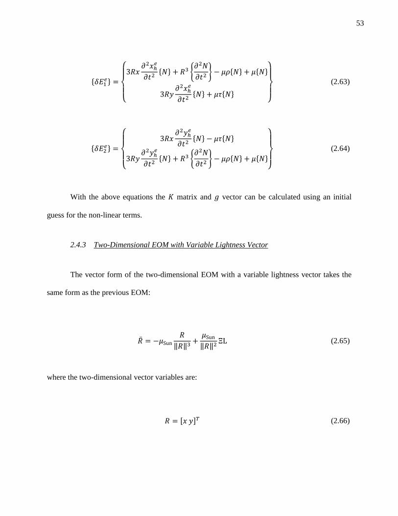
2.4.3 Two-Dimensional EOM with Variable Lightness Vector ........................................................................... 53

2.4.4 Two-Dimensional EOM with Variable Attitude ........................................................................................ 56

2.4.5 Two-Dimensional EOM with Planetary Gravity ........................................................................................ 60

2.4.6 3D EOM without Planetary Gravity .......................................................................................................... 64

2.4.7 Three-Dimensional EOM without Thrust .................................................................................................. 66

viii

2.5 Numerical Solution Details ......................................................................................................................... 69

2.5.1 Boundary Conditions ................................................................................................................................ 69

2.5.2 Time Domain and Step Size ...................................................................................................................... 70

2.5.3 Constants .................................................................................................................................................. 70

2.5.4 Input of Known Variables ......................................................................................................................... 70

3. TRAJECTORY PROPAGATION PROCEDURE ........................................................................ 73

3.1 Overview of STAR ....................................................................................................................................... 73

3.2 Routines ..................................................................................................................................................... 74

3.2.1 Input ......................................................................................................................................................... 74

3.2.2 Planetary Ephemerides............................................................................................................................. 76

3.2.3 Calculating I, K, and g ................................................................................................................................ 76

3.2.4 Newton's Linear Method .......................................................................................................................... 77

3.2.5 Post Processing ......................................................................................................................................... 78

4. TRAJECTORY PROPAGATION RESULTS ............................................................................... 79

4.1 IKAROS Simulation - SRP Acceleration ........................................................................................................ 79

4.2 AKATSUKI Simulation – Three-Dimensional EOM ....................................................................................... 83

4.3 Convergence Study ..................................................................................................................................... 93

4.4 Two-Dimensional Trajectory with Variable Lightness Vector ...................................................................... 95

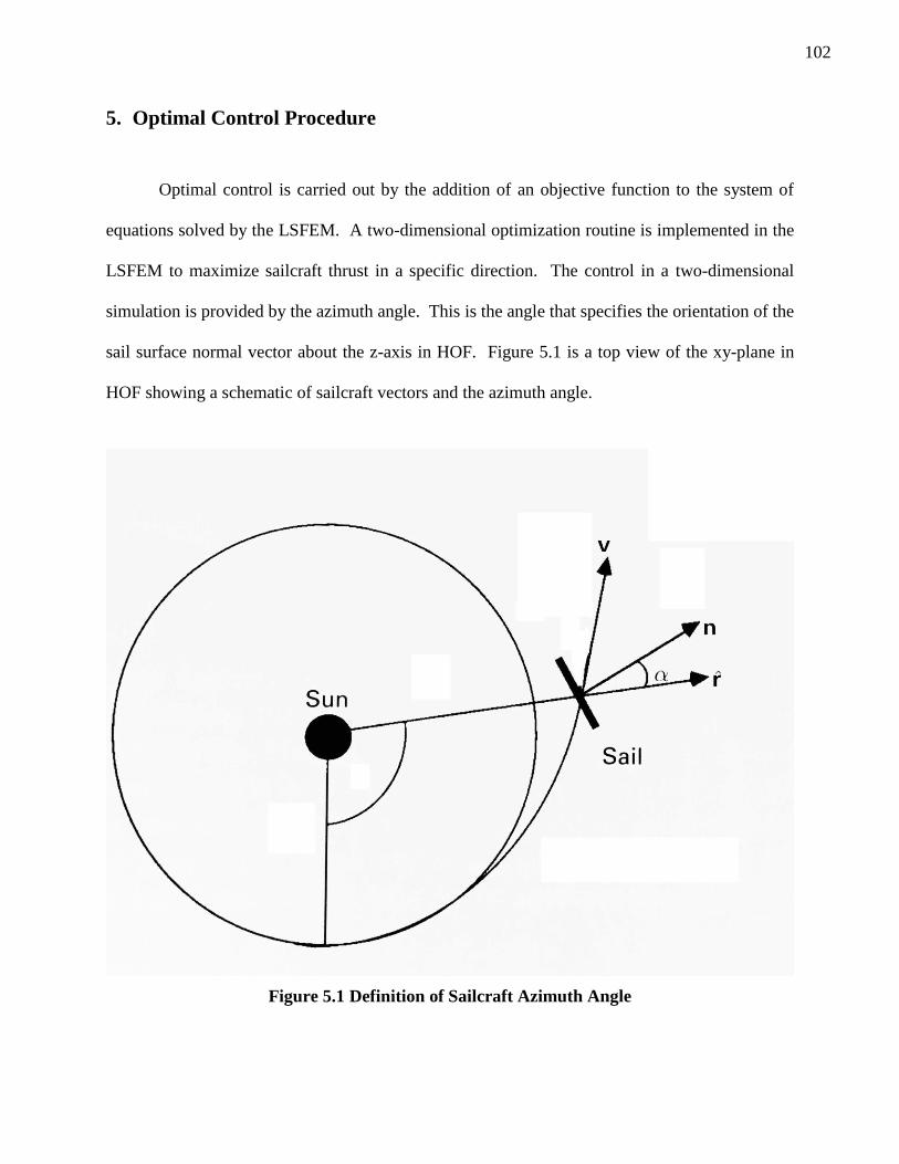
5. OPTIMAL CONTROL PROCEDURE ...................................................................................... 102

5.1 Objective function .................................................................................................................................... 103

ix

5.2 Attitude Adjustment Torques ................................................................................................................... 103

6. OPTIMAL CONTROL RESULTS ............................................................................................. 104

6.1 Thrust Optimization .................................................................................................................................. 104

6.2 Torque ...................................................................................................................................................... 108

7. CONCLUSION .............................................................................................................................. 110

7.1 Impacts and accomplishments .................................................................................................................. 111

7.2 Future Research ........................................................................................................................................ 112

8. REFERENCES .............................................................................................................................. 114

APPENDIX A: FINESSE INPUT FILE ................................................................................................... 1

APPENDIX B: TWO-DIMENSIONAL SIMULATION WITH PLANETARY GRAVITY .............. 1

APPENDIX C: HORIZONS INPUT AND OUTPUT ............................................................................ 1

x

LIST OF FIGURES

Figure 1.1 Effects from light impinging the sail surface [7] ........................................................... 6

Figure 1.2 Stages of IKAROS Sail Deployment [10] ..................................................................... 9

Figure 1.3 Schematic of IKAROS Sail Surface [11] .................................................................... 10

Figure 1.4 Photo taken of a section of the IKAROS sail [11] ...................................................... 10

Figure 1.5 Summary of Solar Sail Research ................................................................................. 11

Figure 2.1 Resultant force vectors from Sunlight on a sail........................................................... 20

Figure 2.2 Magnitudes of accelerations experienced by IKAROS ............................................... 30

Figure 2.3 Objective Functions ..................................................................................................... 35

Figure 3.1 Flow Chart of STAR Code .......................................................................................... 74

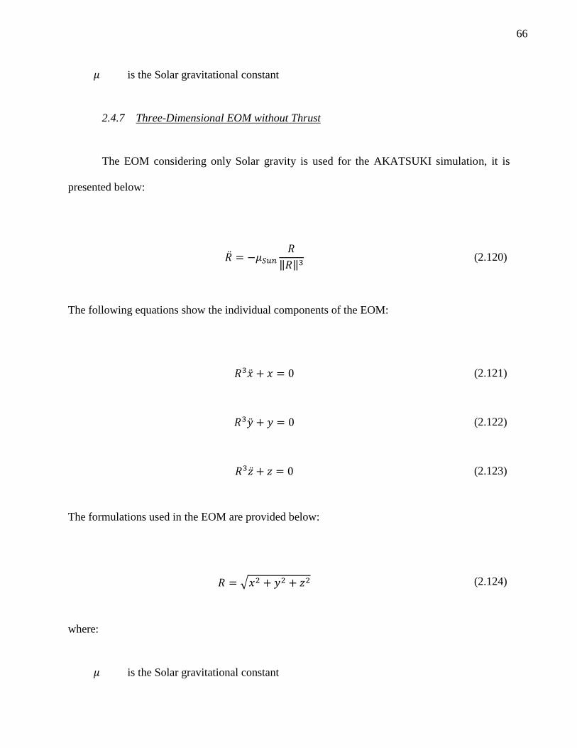
Figure 4.1 Velocity from SRP after IKAROS Sail Deployment [10]........................................... 79

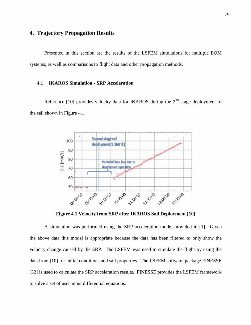
Figure 4.2 Comparison of LSFEM to Flight Data for SRP Acceleration Model ......................... 82

Figure 4.3 L2-norm versus Degrees of Freedom for IKAROS Simulation .................................. 83

Figure 4.4 LSFEM Results and Flight Data of AKATSUKI Trajectory ...................................... 88

xi

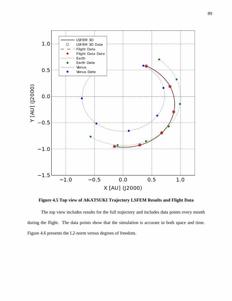
Figure 4.5 Top view of AKATSUKI Trajectory LSFEM Results and Flight Data ...................... 89

Figure 4.6 L2-norm versus Degrees of Freedom for AKATSUKI Simulation ............................ 90

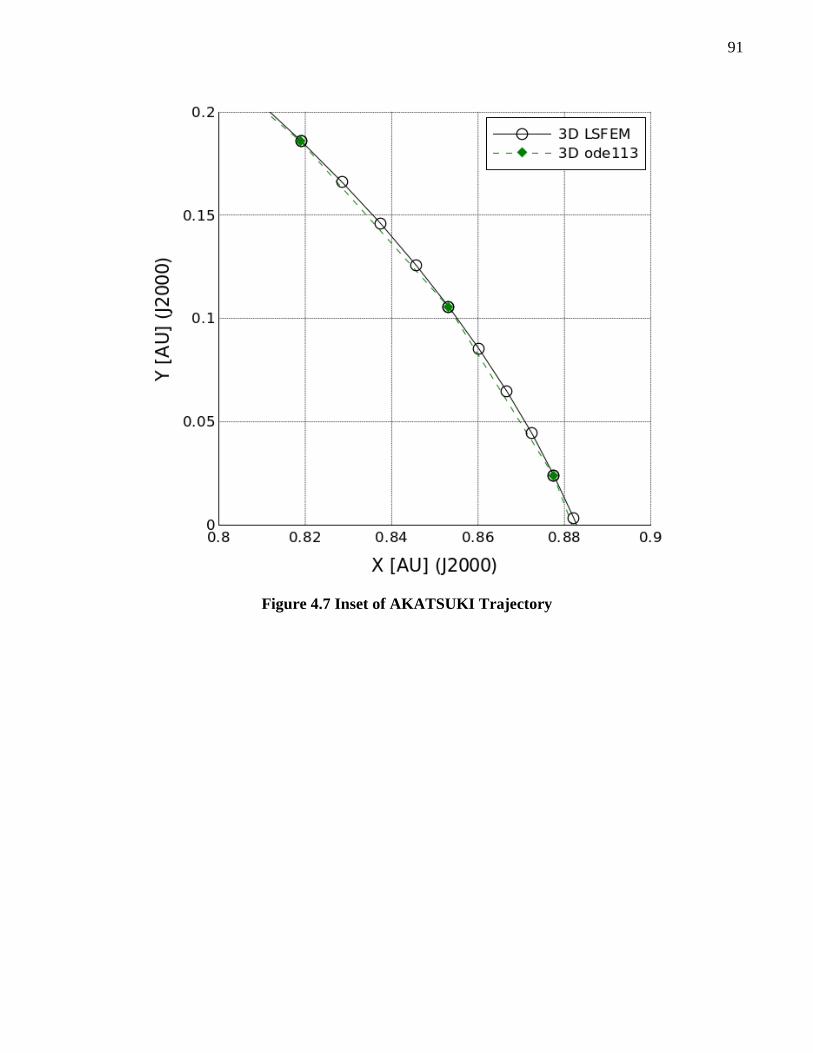
Figure 4.7 Inset of AKATSUKI Trajectory .................................................................................. 91

Figure 4.8 Inset of AKATSUKI Velocity ..................................................................................... 92

Figure 4.9 Convergence Studies of 1D and 3D Simulations ........................................................ 94

Figure 4.10 History of Lightness Vector Components ................................................................. 96

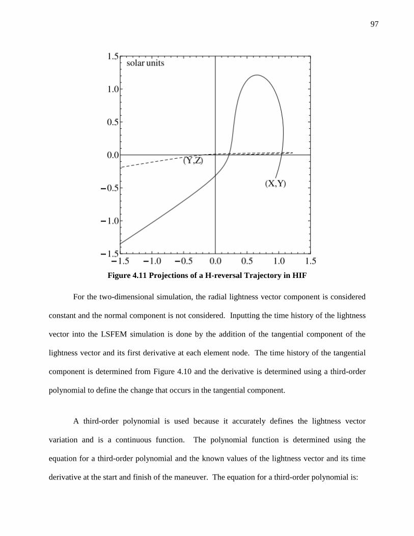
Figure 4.11 Projections of a H-reversal Trajectory in HIF ........................................................... 97

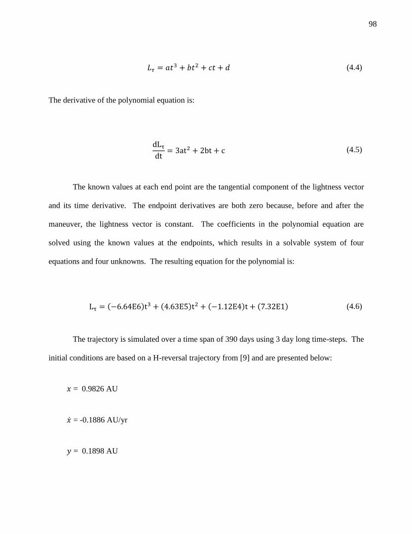
Figure 4.12 Change in Tangential Component of Lightness Vector .......................................... 100

Figure 4.13 Derivative of the Change in Tangential Component of Lightness Vector .............. 100

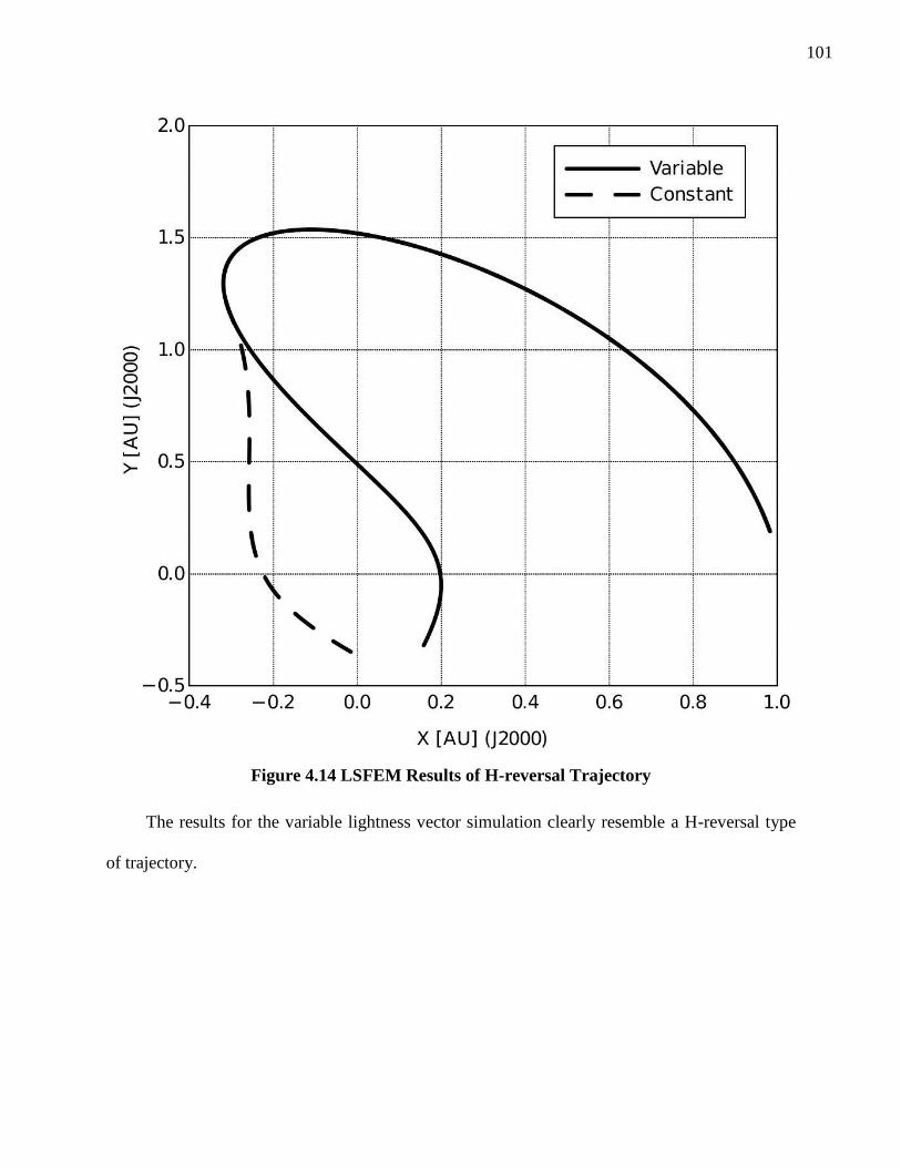
Figure 4.14 LSFEM Results of H-reversal Trajectory ................................................................ 101

Figure 5.1 Definition of Sailcraft Azimuth Angle ...................................................................... 102

Figure 6.1 Objective Function for Thrust Maximization at 30° Azimuth .................................. 105

Figure 6.2 Azimuth Angle of Sailcraft for Thrust Maximization ............................................... 106

Figure 6.3 Azimuth Angular Rate of Sailcraft for Thrust Maximization ................................... 107

xii

Figure 6.4 Azimuth Angular Acceleration of Sailcraft for Thrust Maximization ...................... 107

Figure 6.5 Trajectory for Thrust Optimization ........................................................................... 108

Figure 6.6 Torque for Thrust Optimization Maneuver ............................................................... 109

xiii

LIST OF TABLES

Table 1.1 Comparison of ODE Integration Methods [19][22][23] ............................................... 16

Table 4.1 AKATSUKI Trajectory Flight Data [26] ...................................................................... 85

Table 4.2 AKATSUKI Velocity Flight Data [26] ........................................................................ 86

Table 4.3 Final Data Points for LSFEM Simulation..................................................................... 93

Table 4.4 Final Data Points for ABM Simulation ........................................................................ 93

Table 4.5 Summary of Errors between LSFEM and ABM for AKATSUKI Trajectory .............. 93

Table 4.6 Time History of Lightness Vector Components and Derivatives ................................. 99

xiv

LIST OF SYMBOLS

ACRONYMS

Symbol Description

ABM Adams-Bashforth-Moulton

AU Astronomical Unit

BVP Boundary Value Problem

DOF Degrees of Freedom

EOM Equation of Motion

FEM Finite Element Method

GDE Governing Differential Equation

GNC Guidance, Navigation, and Control

HIF Heliocentric Inertial Frame

HOF Heliocentric Orbital Frame

IKAROS Interplanetary Kite-craft Accelerated by Radiation of the Sun

IVP Initial Value Problem

JAXA Japan Aerospace Exploration Agency

JPL Jet Propulsion Laboratory

LSFEM Refers to Least Squares hpk Fintie Element Method

ODE Ordinary Differential Equation

RCD Reflectance Control Devices

RHS Right Hand Side

SRP Solar Radiation Pressure

xv

STAR Sailcraft Trajectory Analysis Routine

TSI Total Solar Irradiance

VC Variationally Consistent

SYMBOLS

Symbol Description Units

𝐴 Sail area 𝑚2

𝐴 Differential operator ~

𝐴𝑓 Absorptance coefficient ~

𝑎 Acceleration 𝐴𝑈 𝑦𝑟2⁄

𝑐 Speed of light 𝐴𝑈 𝑦𝑟⁄

𝐸 Residual ~

𝐸 Total eneregy 𝑁 ∙ 𝑚

𝑓 Non-homogeneous term in BVP ~

𝐺 Gravity acceleration term 𝐴𝑈 𝑦𝑟2⁄

𝑔 First variation of the residual function ~

ℎ Direction of angular momentum vector ~

𝐼 Residual functional ~

𝐼 Sailcraft moment of inertia 𝑘𝑔 ∙ 𝑚2

𝐽0 Radiant energy per unit area per unit time 𝑊 𝑚2⁄

𝐾 Coefficient matrix ~

𝐿 Lightness vector ~

xvi

𝐿1𝐴𝑈 Length of one AU 𝑘𝑚

𝐿𝑆 Solar luminosity 𝑁 ∙ 𝑚/𝑠

𝑚 Mass 𝑘𝑔

𝑁 Approximation function ~

�⃗� Direction of the sail surface normal vector ~

𝑃 Pressure 𝑁 𝑚2⁄

𝑝 Momentum 𝑘𝑔 ∙ 𝑚 𝑠⁄

𝑝 Planetary term ~

𝑝 Polynomial degree ~

𝑅 Distance from the Sun 𝐴𝑈

𝑅 Vector location in HIF 𝐴𝑈

ℜ Reflectance coefficient ~

𝑟 Direction vector in HIF ~

𝑡 Time 𝑦𝑟

�⃗� Direction of the sailcraft location vector ~

𝑇 Control torque 𝑁 ∙ 𝑚

𝑉 Velocity vector in HIF 𝐴𝑈/𝑦𝑟

𝑊 Radiant energy flux 𝑁 𝑚 ∙ 𝑠⁄

𝑥 x-component of location sailcraft in HIF 𝐴𝑈

𝑥𝑠⃗⃗ ⃗ Direction of the sailcraft x-axis in HOF ~

𝑦 y-component of location sailcraft in HIF 𝐴𝑈

𝑧 z-component of location sailcraft in HIF 𝐴𝑈

xvii

GREEK SYMBOLS

Symbol Description Units

𝛼 Iteration parameter for Newton's method ~

𝛼 Sailcraft azimuth Angle deg

β̃ Angle from diffuse momentum vector to the x-axis of the sail in HOF ~

β(f) Reflection constant ~

𝛾 Absorption coefficient ~

𝛿 Degree of freedom vector ~

휀 Surface emittance ~

𝜂 Normal component of lightness vector ~

𝜅 Sail material emissivity ~

𝜇 Gravitational parameter 𝑘𝑚3

𝑠2

𝛯 Transformation matrix from HOF to HIF ~

𝜉 Independent variable in natural coordinate space ~

𝜌 Radial component of lightness vector ~

𝜎 Sailcraft loading 𝑘𝑔 𝑚2⁄

𝜏 Tangential component of lightness vector ~

𝜏𝑦𝑒𝑎𝑟 Seconds in a year 𝑠 𝑦𝑟⁄

𝜐 Sun incidence angle 𝑟𝑎𝑑

𝜑 Differential equation variable ~

𝜒 surface emission/diffusion coefficient ~

xviii

𝛺 Domain of integration ~

𝜔 Angular velocity 𝑟𝑎𝑑/𝑠

�̇� Angular acceleration 𝑟𝑎𝑑/𝑠2

SUBSCRIPTS

Symbol Description

b Back

cr Critical

d Diffuse

e Element

f Front

h Approximated variable

opt Optimum

p Planet

p-s Value between planet and Sun

s Specular

1

1. INTRODUCTION

Presented in this section is an overview of the research topic, which includes the

motivation of the research, brief details of solar sail spacecraft, and a summary of related topics.

1.1 Overview

The following subsections explain the research and the purpose for conducting the

research.

1.1.1 Motivation

Solar sail spacecraft accelerate payloads through space using zero propellant. Their

source of thrust is provided from an abundant and practically free source of energy, the Sun.

They utilize the Sun as a constant source of thrust to push them through our solar system. The

new method for solving the sailcraft EOM will help increase the success rate of solar sail

missions. It will help by providing numerical solutions that are true to the physics of sailcraft

trajectories and also provide a priori error analysis.

Recently, the Japan Aerospace Exploration Agency (JAXA) sent a sailcraft named

Interplanetary Kite-craft Accelerated by Radiation Of the Sun (IKAROS) on a mission to

demonstrate sailcraft technologies. It successfully completed its mission to Venus proving that

sailcraft are a realistic option for space travel. During its mission, IKAROS returned tracking

data that show clear evidence that SRP was producing thrust and providing attitude control for

the sailcraft. The next solar sail spacecraft, named LightSail, produced by The Planetary

2

Society, will launch in May of 2015 [1]. Its initial mission is a test flight to test the sail

deployment sequence. A full solar sailing demonstration mission is set to launch in 2016. The

upcoming launch of LightSail and the success of IKAROS show the current interest in sailcraft

as a viable option for space travel. A summary of sailcraft missions is presented below:

IKAROS launched by JAXA on May 21, 2010. It set a world record for becoming the first

solar sail spacecraft to complete an interplanetary flight. IKAROS confirmed acceleration

was achieved by a solar sail. [2]

NanoSail launched by NASA on November 19, 2010. It was deployed in low-Earth orbit to

demonstrate the deorbit capabilities of solar sails. [3]

Cosmos 1 was produced by the planetary society and launched on June 21, 2005. It failed to

reached orbit due to a launch vehicle failure. [4]

LightSail mission one will be launched by The Planetary Society in May 2015. It will

perform a test flight to determine how the sail will acts in a microgravity environment. [5]

LightSail mission two will be launched by The Planetary Society in 2016. It will

demonstrate the solar sailing capabilities of the spacecraft. [7]

The above list shows how solar sails are becoming a relevant source of propulsion for spacecraft.

To date, the data from the IKAROS mission is the only thrust data recorded for a

sailcraft, therefore, the amount of experimental data related to sailcraft is scarce. Gaining more

flight data requires extreme expenses of both time and money. Therefore, to efficiently design

3

and analyze sailcraft, an accurate and reliable computational simulation is needed. The new

approach presented here has the aim of filling this need by using the most up-to-date sailcraft

equations of motion coupled with an advanced numerical solver.

The numerical solver is a high-accuracy finite element method called the hpk least

squares finite element method (LSFEM). The LSFEM incorporates high order global

differentiability, high order polynomial approximations, and exact determination of numerical

errors into the numerical framework. These numerical advantages give the LSFEM the ability to

provide solutions that are more true to the physics of sailcraft motion.

1.1.2 Objective

A new approach is presented that combines the LSFEM with the sailcraft equations of

motion to achieve an accurate and reliable method for the design and analysis of sailcraft

missions. The mathematical model of the sailcraft EOM includes terms for SRP, attitude

changes, planetary perturbations, and solar gravity, but it has the potential to include all physical

aspects of the sailcraft motion. These include sail material degradation and relativistic affects.

The solution to the sailcraft EOM needs to be solved numerically due to the non-linear

nature of the ODE system. The research presented herein shows that the LSFEM has been found

to be a superior method. The LSFEM is setup to time-march through the duration of the

simulation, while providing simultaneous solutions of the sailcraft location, velocity,

acceleration, and, if applicable, attitude angles, rates and accelerations. The data from the

simulations will be compared to the flight data of the IKAROS sailcraft to verify the accuracy of

the results. Simulations are also presented for non-sail spacecraft to show the additional

4

capabilities of the new method.

The new method separates itself from other propagation methods by the following

features:

Unconditionally stable numerical solution for non-linear EOM

Improved physical description through the inclusion of derivatives in the DOFs

A priori error estimation at any point in the solution domain

Provides control input for optimizing thrust

The new trajectory propagation method is extended further with the addition of optimal

control. An additional equation is added to the EOM system to maximize thrust in a specific

direction. The LSFEM formulation inherently provides a minimization within the computational

framework. This is utilized to minimize an objective function that is created to maximize thrust.

Outputs of the optimal control solution are the sailcraft location, velocity, acceleration, attitude

angle, angular rate, and angular acceleration. The angular outputs are placed into the spacecraft

attitude dynamics equations to determine the torque required to maneuver the sailcraft to the

maximum thrust position.

Technical details of the EOM and LSFEM are presented, as well as the process of

implementing the EOM into the LSFEM. The procedure for running the simulations and

optimization are also presented, along with results for each simulation.

5

1.1.3 Practical Purpose

A key step in the design and analysis process for spacecraft involves propagating the

trajectory. Trajectory propagation is the process of solving the EOM through a specified span of

time. This is done for a number of reasons including simulating the flight path and validating

design parameters. The approach to solving EOMs presented in this research acts as a

replacement or a supplement to the current sailcraft trajectory propagation techniques.

1.2 Sailcraft

1.2.1 General Description

Solar sail spacecraft, or sailcraft, use light as their source of propulsion. The force

resulting from the impinging light on the sail will continue as long as light is allowed to irradiate

the surface of the sail. The amount of force exerted on the sailcraft depends on the surface area

and surface material of the sail. The distance of the sail from the Sun also affects the amount of

thrust produced by the sail. Thrust is approximately proportionate to the inverse square of the

distance between the Sun and the sail. For a sail the size of IKAROS, at 1 AU, the thrust is on

the order of 1 mN. Compared to the 91 mN [6] produced by the ion thrusters of the Dawn

spacecraft, the sailcraft thrust is small. However, IKAROS is considered a small sailcraft based

on its sail area of 196 m2. Current sailcraft concepts increase thrust using larger sails and flight

paths with close proximity to the Sun.

Force on the spacecraft is the result of momentum transported to the surface of the sail by

electromagnetic radiation from the Sun. In the quantum description, light photons irradiate the

6

sail surface causing a momentum transfer. Using the electromagnetic description, the

momentum transfer is the result of the sail interacting with radiation from electromagnetic

waves. Mathematically speaking, both descriptions provide equivalent values for solar radiation.

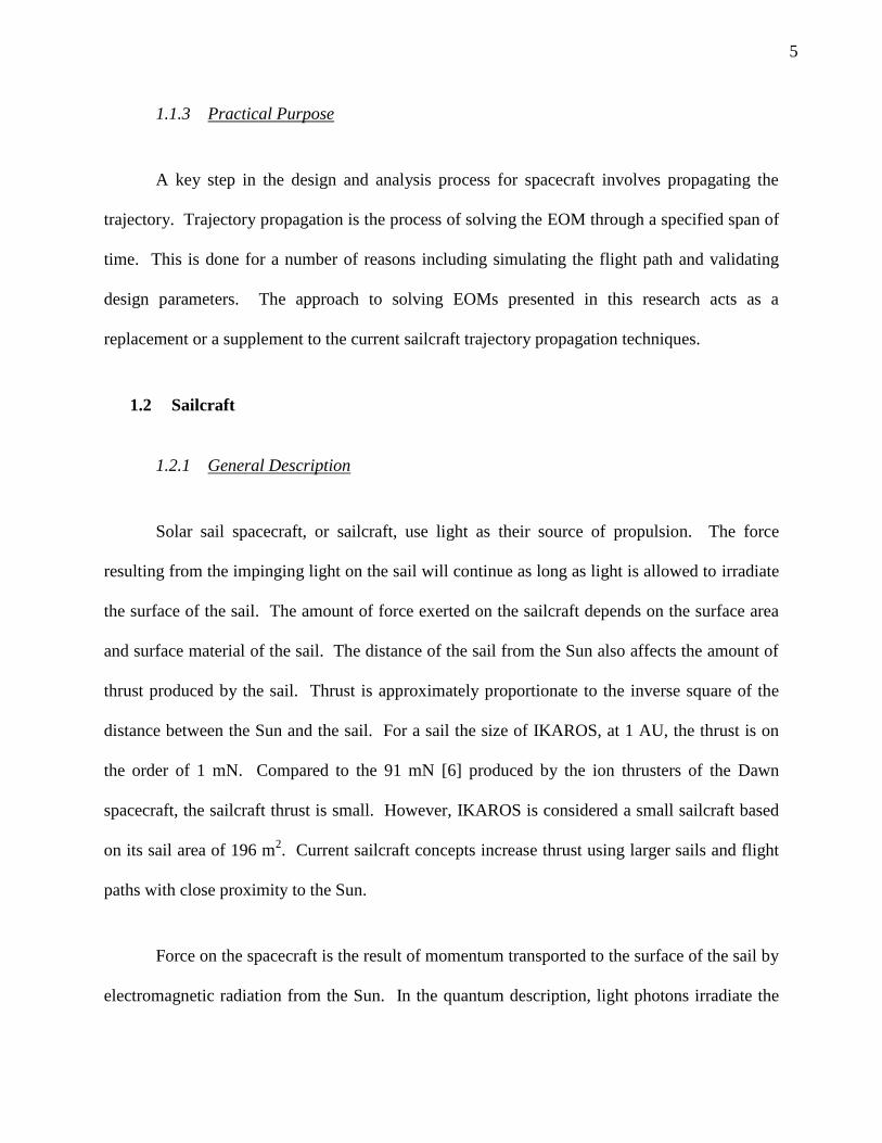
Once the radiation impinges on the surface of the sail it does one of four things: reflects

spectrally, reflects diffusively, absorbs into the sail, or transmits through the sail. Figure 1.1

displays these interactions.

Figure 1.1 Effects from light impinging the sail surface [7]

The appearance of a sailcraft, which is based on maximizing thrust, generally takes the

form of a large, flat square or circle with a relatively small, centralized payload. The large

surface area is made up almost entirely by the sail, which is made of a lightweight, highly

7

reflective material. When Sunlight irradiates a surface it generates solar radiation pressure

(SRP), thus thrust is the result of SRP acting on the sail. Keeping the sailcraft mass low results

in a greater amount of acceleration for a given amount of thrust, which makes sail material and

thickness key design variables. Attitude control can come from changing the orientation of

certain parts of the sail, or in the case of IKAROS, by using variable reflectance panels

positioned on the surface of the sail. The amount of SRP increases exponentially as the distance

between the sailcraft and the Sun decreases.

Equations for the momentum transfer caused by solar radiation are briefly described

below and will also be described in detail in subsequent sections. Equation (1.1) from [8] is one

of the first presentations of quantifying SRP on spacecraft and it shows the relation between

acceleration from SRP and distance from the sun.

𝑎𝑆𝑅𝑃 =𝑘

𝑟𝑆𝑢𝑛2

(1.1)

where:

𝑎𝑆𝑅𝑃 is the acceleration from SRP

𝑟𝑆𝑢𝑛 is the distance from the Sun

k is a constant representing Sunlight properties, spacecraft mass, spacecraft surface

area,and spacecraft optical properties

Despite its simplicity, Equation (1.1) shows how the position of the spacecraft and the

8

spacecraft physical properties affect the amount of SRP acceleration.

The sailcraft equation of motion from [9] in vector form is presented below in Equation

(1.2).

�̈� = 𝐺𝑆𝑢𝑛 + 𝐴 +∑𝐺𝑝𝑝=1

(1.2)

where:

�̈� is the sailcraft acceleration

𝐺𝑆𝑢𝑛 is the acceleration due to gravity from the Sun

A is the acceleration from the SRP

∑ 𝐺𝑝𝑝=1 is the sum of accelerations from planetary gravity

This equation states that as the sailcraft travels through the solar system it experiences

forces from the Sun's gravity, nearby planetary gravity, and SRP acting on the sail.

1.2.2 The IKAROS Sailcraft

The IKAROS sailcraft was produced and launched by JAXA with the purpose of

demonstrating technologies of the sailcraft concept for future missions. The main concepts

demonstrated during the mission were in-space sail deployment, power generation using solar

9

cells on the sail, thrust from SRP, and guidance and navigation capabilities of a sailcraft. Its

launch took place on May 21, 2010 at the Tanegashima space center aboard the H-IIA rocket as a

piggy-back payload of the AKATSUKI Venus climate orbiter [10]. Once IKAROS was injected

into the Venus transfer trajectory, it separated from the rest of the payload and began its 180 day

trip to Venus. Shortly after separation, the 20 m-span sail was deployed. To deploy the sail, the

sailcraft spun about its central axis while releasing tip masses at the four corners of the square

sail, the centrifugal force slowly drew the sail outward until it was fully deployed. Figure 1.2

provides a visualization of each step of the sail deployment.

Figure 1.2 Stages of IKAROS Sail Deployment [10]

The sail of IKAROS has a mass of 16 kg, an area of 196 m2 and a minimum thickness of

7.5 μm The total mass of the spacecraft is 307 kg. The sail weight is kept low as a result of

using the centrifugal force of the tip masses to keep the sail extended instead of using support

structure. Located on the sail surface are solar panels for power generation and reflectance

control devices (RCD) for attitude control. The location of these devices is shown in the

10

schematic in Figure 1.3 and the photograph of the sail in Figure 1.4.

Figure 1.3 Schematic of IKAROS Sail Surface [11]

Figure 1.4 Photo taken of a section of the IKAROS sail [11]

The RCDs are flexible sheets made of encapsulated liquid crystal. When electrical

voltage is applied to the sheets, the optical reflectance changes between specular and diffuse.

When these changes of reflectance are synchronized with the spinning phase of the sailcraft, they

change the spin axis of the sailcraft without using any propellant.

To prove the concept of using SRP for thrust, Doppler measurements were used to record

the sailcraft trajectory and provide data for the amount of SRP thrust that the sail was providing.

An accumulated velocity of over 100 m/s was recorded after the six month cruise to Venus.

11

After deployment, a thrust force of 1.12 mN was measured. Also recorded was the velocity of

the sailcraft immediately following the deployment of the sail, which will be used for verifying

the simulation later in this document. IKAROS successfully completed its Venus flyby mission

on December 8, 2010.

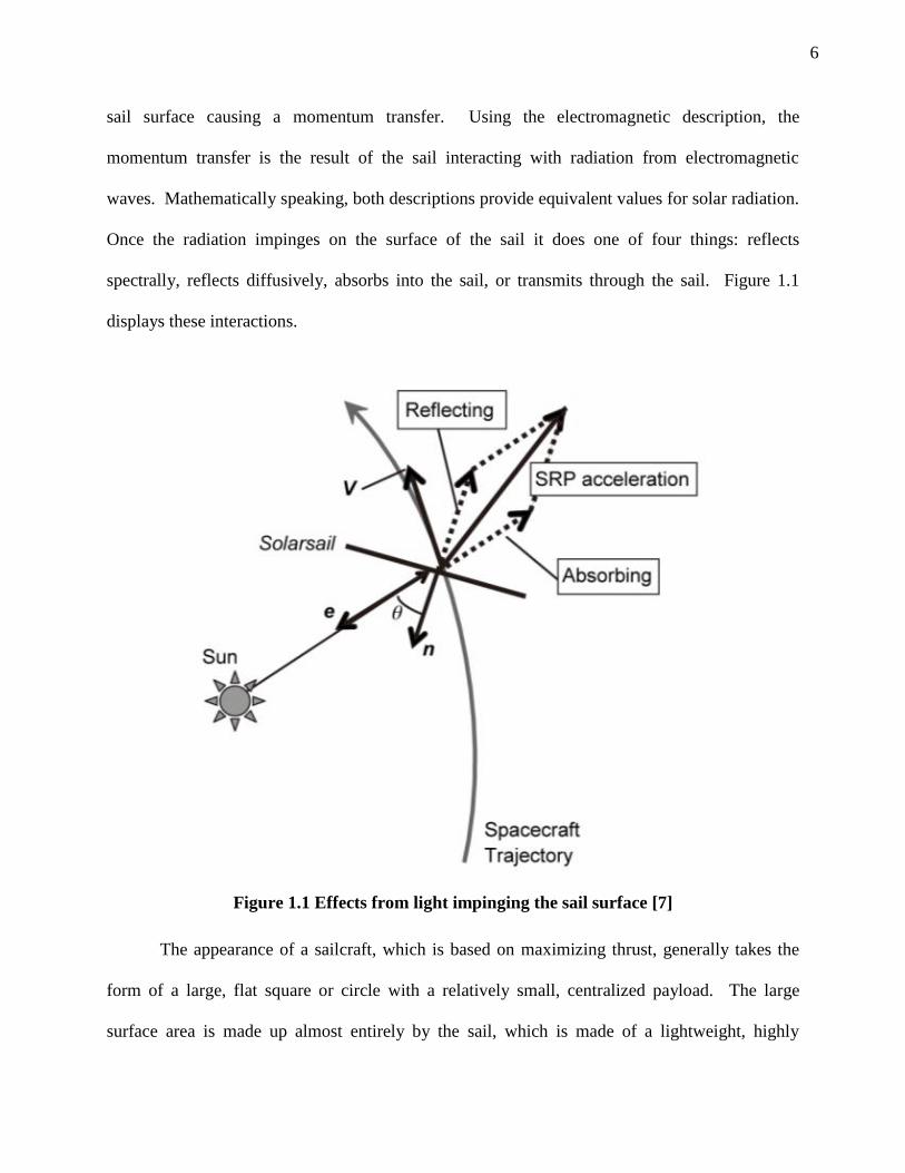
1.3 Literature Review

Similar research has been reviewed to help expand the capabilities of the new method and

to present comparison between methods currently in use. The flow chart shown in Figure 1.5

summarizes the history of sailcraft research.

Figure 1.5 Summary of Solar Sail Research

12

1.3.1 Mathematical Models of the Sailcraft Motion

The work of F[8] presents a solar radiation pressure mathematical model. Its purpose is

to provide an accurate model to calculate the spacecraft forces and torques for high-precision

attitude control. The model takes into account spacecraft mass, irradiated surface area, incident

and reflected light, absorbed light, and distance from the Sun. The outcome is an equation for

SRP that is a function of the spacecraft's distance from the Sun and the spacecraft's physical

properties. Compared to Sun-centered EOMs, this model is relatively simple because it uses the

spacecraft reference frame and only accounts for SRP force. Despite its simple nature, it is the

foundation for the more advanced models.

The work presented in [8] is expanded in [12] to become a three-dimensional, sailcraft-

specific SRP thrust model. SRP is calculated similar to the model in [8], however, the terms for

the material constants are more detailed and the attitude of the sailcraft with respect to the Sun is

considered. The inclusion of solar gravity results in a more complicated EOM due to the

coordinate transformation required between the Sun-centered and sailcraft-centered reference

frames. The outcome of the model is a sailcraft EOM based on accelerations from SRP, solar

gravity, and planetary gravity. The final form of the EOM is a non-linear, second order ODE.

Also in [12] is a description of how sailcraft in close proximity to the Sun (within 10 solar radii

of the Sun, or 0.047 AU,) will experience a decrease in SRP due to the non-parallel incidence

angles of the photons. Temperature of the sail is also addressed.

A generalized sail model is developed in [13]. It uses the SRP equation from [12] to

determine the forces on an arbitrary, fixed sail geometry. The model requires knowledge of the

normal direction of the entire sail surface with respect to the sail-fixed reference frame, which

13

accounts for the changes in force vector caused by surface geometry. The normal directions of

the sail surface come from splitting the sail into smaller flat surfaces. Force on the sail is

calculated using radiation pressure, optical properties, sail surface normal vectors, and the solar

incidence vector. The model is simplified using constants for geometric and optical properties,

however, it becomes more complex when sailcraft attitude is considered.

Most recently [9] has provided the most detailed EOM for sailcraft thus far. Like the

previous EOMs, this version is three-dimensional, includes sail material properties, uses a

coordinate transformation from the Heliocentric Orbital Frame (HOF) to the Heliocentric Inertial

Frame (HIF), and includes acceleration terms for SRP, solar gravity, and planetary gravity. It

can also be formulated to consider non-flat sail geometry similar to the model in [13] and

degradation of sail optical properties. Details of sail material properties include surface

roughness, reflection and transmission profiles, and mean surface behavior. These

characteristics are quantified for use in thrust calculations. Introduced in the text is the lightness

vector, which acts as a scaling factor in the sailcraft EOM for the flat-sail model by scaling the

SRP acceleration to the gravitational acceleration of the Sun, or central body. Also presented are

approaches for trajectory optimization and the theory of fast solar sailing.

1.3.2 Numerical Trajectory Propagation

In the sailcraft software presented in [14] trajectory propagation is calculated using three

numerical integration techniques: Adams-Bashforth-Moulton, Bulirsch-Stoer, and Runge-Kutta-

Shank. The Runge-Kutta-Shanks method is a higher order version of the traditional Runge-Kutta

method based on the Taylor series. Adams-Bashforth-Moulton is a mutli-step method that uses a

predictor corrector technique. Details of these techniques are presented in the following

14

subsection.

Presented in [15] is a software toolkit developed specifically for sailcraft mission design

and GNC analysis. It contains five primary modules that are each capable of calculating separate

details of the simulation that combine to provide details of a sailcraft mission simulation. Of

particular interest are the sections outlining the details of the SRP module and the orbit

determination module, which is referred to as DET. The SRP module uses the models presented

in [12] and [13] to provide thrust and torque data. The sailcraft equations of motion are handled

by the DET module, which calculates the trajectory evolution by integrating the EOM.

Reference [16] presents a sailcraft simulation toolbox designed to act as a single piece of

software that handles all aspects of sailcraft design and analysis. The simulation toolbox uses a

MATLAB based ODE solver named 'ode113' to propagate the trajectories. [17] states that this

integration sub-routine is based on the Adams-Bashforth-Moulton method.

1.3.3 Numerical Integration Methods

Sailcraft equations of motion, like most spacecraft equations of motion, take the form of a

system of non-linear, second order differential equations. Equations of this nature generally

have no analytical solution, however, the use of numerical integration techniques provides

reasonable approximations of such equations. All of the available techniques, in some way,

convert the ODE into a system of algebraic equations, and the solution of the system provides an

approximate solution to the ODE. The steps used to arrive at the algebraic system are what make

each technique unique.

15

In astrodynamics, numerical integration techniques are used to propagate spacecraft

trajectories, in other words, they provide numerical solutions to spacecraft EOMs. Based on [14]

and [16], common techniques are Runge-Kutta-Shanks , Bulirisch-Stoer, and Adams-Bashforth-

Moulton. In all cases, the techniques can only solve a system of first order ODEs. Handling

high order ODEs requires a rework of the EOMs or multiple integrations per step. This

introduces an increased amount of error at each step. Also, due to the nature of the numerical

techniques, there is no calculation of the exact error of the entire trajectory. At best, there errors

are only known at each time step. Each technique uses either a single-step or multi-step

methodology. Single-step are simple yet relatively inaccurate. Multi-step methods have high

accuracy compared to single-step methods of the same order and are recommended for long-

duration simulations. Also, multi-step methods usually require data from a set of previous step,

single-step methods are often used to initialize this data set. Order of accuracy for each method

depends on the order of the Taylor series expansion used to formulate the algebraic system.

Below is a brief review of the techniques found in sailcraft literature and techniques

commonly used in astrodynamic problems. The Runge-Kutta-Shanks method from [18] is an

improvement on the Runge-Kutta method by means of allowing high order approximations up to

the eighth order. The method is self-starting, therefore it requires only one set of initial

conditions. Like similar methods, a second order ODE must be split into a system of first order

ODEs.

Reference [19] reveals that the Burlisch-Stoer reduces computer time but it has reliability

issues. The Adams-Baschforth-Moulton technique uses a predictor-correcter, or mulit-step,

method. It requires a series of initial conditions and, therefore, is not self-starting. To obtain the

16

set of initial conditions, a Runge-Kutta method with matching order is generally used. Similar to

the Runge-Kutta-Shanks method mentioned above, higher order ODEs need to be integrated

twice or separated into a system of equations.

In the simulation toolkit presented in [16], the MATLAB subroutine 'ode113' was used to

integrate the EOM. [17] states that this subroutine implements the Adams-Bashforth-Moulton

technique described above.

Presented in [20] and [21] is an advanced version of the finite element method, which is

the numerical technique used for solving the sailcraft EOM for this research. This implicit form

of the FEM uses high order polynomials to approximate the equation variables. Higher order

global differentiability is implemented into the polynomial approximations, which provides

solutions for the variables and their derivatives simultaneously. ODEs of any order can be

solved as long as the appropriate initial conditions are provided. The required initial conditions

are the same for solving any ODE analytically and are based on order of the equation and

number of variables. A detailed description of the method is provided in Section 2.3.

Table 1.1 compares different common ODE integration methods to the LSFEM.

Table 1.1 Comparison of ODE Integration Methods [19][22][23]

Method

Unconditionally

Stable

Self

Starting

A Priori Error

Estimation

Continuous

Solution

High Order

Systems

LSFEM Yes yes yes yes yes

Runge-Kutta Yes yes no no no

Adams-Bashforth-

Moulton No no no no no

Burlisch-Stoer No no no no no

The numerical solution of the LSFEM can be trusted because it is variationally consistent and the

17

error between the numerical solution and the theoretical solution is known. For other methods to

be trustworthy, there must be knowledge of the equilibrium points, the nature of the solution, and

the stability properties [23].

1.3.4 Determination of EOM Variables and Parameters

Estimating the sail optical parameters is a required step in computing the EOM. [24]

presents numeric computations of the specular reflectance, diffusive reflectance, and absorptive

parameters of aluminum. Data for aluminum is relevant because most sailcraft designs use an

aluminum coated membrane for their sail material. Computations in [24] are based on

experimental data of an aluminum film similar to the type used on sailcraft. The results show

values for the three parameters as functions of photon incidence angle for varying thicknesses of

aluminum.

1.3.5 IKAROS Flight Data

Presented in [25] is a description of the IKAROS sailcraft and its purpose, which is to

demonstrate the capabilities of a solar sail spacecraft. Provided in the literature are important

details regarding physical aspects of the sail size and material. The demonstration mission of

IKAROS precedes a potential sailcraft mission to Jupiter.

The flight of IKAROS is documented in [10] and [11]. It was launched in 2010 and

deployed its 20 m sail to help propel it to its destination, Venus. Presented in [10] are details of

the mission, the designed trajectory, and most relevant to this research, velocity measurements

taken during and after sail deployment. Velocity data was collected using real time Doppler

18

observation minus calculation measurement during a three hour span, which captured the

acceleration from the SRP. Details of IKAROS attitude, spin rate and attitude control are also

provided in [10].

The content in [11] is similar to that in [10] except the data from IKAROS entire flight is

presented. A key feature of [11] is flight data for the velocity due to SRP during the entire trip to

Venus. The data shows a slight increase in acceleration as the sailcraft nears Venus, which is

likely due to higher levels of SRP from the sailcraft nearing the Sun. Included in [11] are the

time-lines of IKAROS trajectory and attitude during the flight.

19

2. THEORETICAL CONSIDERATION

The following sections describe the physical and mathematical details of the new

trajectory propagation method. Included are details of calculating SRP, construction of the

EOM, the mathematics of the FEM, and implementation of the EOM into the FEM.

2.1 Sailcraft Dynamics

2.1.1 Frames of References

The frames of reference are described in this section to clarify the different coordinate

systems that are utilized in sailcraft dynamics. The two frames of reference used in the model

are the HOF and HIF.

At the origin of the HOF is the barycenter of the sailcraft. Its axes are based on Cartesian

coordinates and orient themselves with respect to the sailcraft and the Sun. The HOF x-axis

extends from the sailcraft to the barycenter of the Sun. The z-axis is given by the direction of the

sailcraft angular momentum vector. Using HOF, sailcraft attitude and elevation angles are

measured from the x-axis using the sailcraft rotation about the z-axis and y-axis, respectively.

During FEM implementation, it is straightforward to handle attitude and elevation in the HOF

frame as opposed to calculating them in HIF.

HIF share's its origin with the Sun's barycenter. The reference plane, or the x-y plane,

uses the mean ecliptic at J2000 and the x-axis is directed along the equinox at J2000.

Simulations presented herein are based in HIF with attitude variables presented in HOF.

20

2.1.2 Modeling Solar Radiation Pressure

SRP is the result of Sunlight impinging on a surface, which causes a momentum transfer

from the light photons to the surface. When incident light shines on a surface, the light does one

of four things, it can reflect spectrally, reflect diffusively, absorb into the surface, or transmit

through the surface. Spectral reflection provides the greatest amount of pressure, followed by

diffuse reflection, then by absorption. When light transmits through a surface, no pressure is

exerted. Pressure from reflected light produces a resultant force normal to the surface. When

light is absorbed, the resultant force is parallel to the incident light. Figure 2.1 shows the force

vectors resulting from Sunlight impinging on the surface of a sailcraft.

Figure 2.1 Resultant force vectors from Sunlight on a sail

Momentum is transferred to the sail from SRP when solar photons impinge on the sail

surface. The effect of the photon interaction is described using the mass energy equivalence of a

moving body from special relativity.

21

𝐸2 = 𝑚02𝑐4 + 𝑝2𝑐2

(2.1)

where:

E is total energy

m0 is mass

c is the speed of light

p is the momentum

The total energy of the moving body is made from two parts, the energy of the body at

rest and the energy due to the motion of the body. For photons, which have zero mass, the first

term disappears, resulting in:

𝐸 = 𝑝𝑐 (2.2)

To calculate pressure generated by photons in motion, the momentum transported by a flux of

photons is related to the total energy.

𝛥𝐸 = 𝑊𝐴𝛥𝑡 (2.3)

where:

W is the radiant energy flux or radiant energy per unit area per unit time

A is the area normal to the incident radiation

22

t is time

Combining these two equations provides:

Δp=WAΔt

c

(2.4)

The definition of pressure, P, related to momentum transport is:

𝑃 =1

𝐴(𝛥𝑝

𝛥𝑡)

(2.5)

Defining P as SRP and combining the previous two equations together gives:

𝑆𝑅𝑃 =𝑊

𝑐

(2.6)

The resulting equation states that SRP is the radiant energy flux divided by the speed of light.

Flux of solar radiation can be scaled based on distance from the Sun using the following

relationships.

𝑊 = 𝑊𝐸 (𝑅𝐸𝑟)2

(2.7)

𝑊𝐸 =𝐿𝑆

4𝜋𝑅𝐸2

(2.8)

where:

LS is the solar luminosity

RE is one astronomical unit

23

R is distance from the Sun

The above relationship is used as part of the formulation for defining SRP as a function of

sailcraft location. To solve the SRP equations, which will be done as part of the sailcraft EOM,

they must be arranged to single out acceleration. When implemented into the LSFEM, the

evolution of the sailcraft location and time derivatives of location will be the solution variables

for a given span of time.

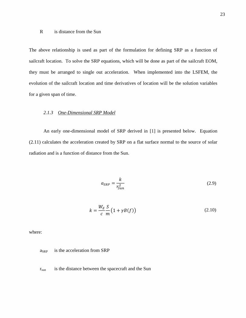
2.1.3 One-Dimensional SRP Model

An early one-dimensional model of SRP derived in [1] is presented below. Equation

(2.11) calculates the acceleration created by SRP on a flat surface normal to the source of solar

radiation and is a function of distance from the Sun.

𝑎𝑆𝑅𝑃 =𝑘

𝑟𝑆𝑢𝑛2 (2.9)

𝑘 =𝑊𝐸

𝑐

𝑆

𝑚(1 + 𝛾𝐵(𝑓)) (2.10)

where:

aSRP is the acceleration from SRP

rsun is the distance between the spacecraft and the Sun

24

WE is the radiant energy per unit area per unit of time at 1 AU

c is the speed of light in a vacuum

S is the surface area of the sail

m is the mass of the entire sailcraft

B(f) is the reflection constant

γ is the absorption coefficient

The acceleration equation clearly shows the inverse square law that governs the

relationship between SRP acceleration and distance from the Sun. When this model is

implemented in the LSFEM, it takes the following form:

𝑑2𝑅

𝑑𝑡2=1

𝑅2𝑊𝐸

𝑐

𝑆

𝑚

𝑡𝑦𝑟2

𝐿1𝐴𝑈(1 + 𝛾𝐵(𝑓)) (2.11)

R is the distance from the Sun and is the only variable.

2.1.4 Three-Dimensional Flat Sail Model

A common method for calculating SRP induced acceleration on a sailcraft is performed

by scaling down the solar gravity at the sailcraft location. The scale factor presented in [9],

25

which is also used for the FEM model presented in this research, is called the lightness vector.

Calculating the magnitude of the solar gravity on the sailcraft is achieved by dividing the solar

gravitational constant by the squared distance from the Sun. To get SRP acceleration, one

simply multiplies the lightness vector by the solar gravity acceleration. Equation (2.12) shows

the formulation.

𝑎𝑆𝑅𝑃 = 𝐿𝜇𝑆𝑢𝑛‖𝑅2‖

(2.12)

where:

L is the lightness vector

μSun is the Solar gravitational constant

R is the position vector of the sailcraft.

L is calculated in HOF, therefore, to determine the SRP acceleration in HIF, L needs to

be transformed from HOF to HIF. The SRP acceleration in HIF is presented below in Equation

(2.13) and Equation (2.14).

𝑎𝑆𝑅𝑃 = 𝛯𝐿𝜇𝑆𝑢𝑛‖𝑅‖2

(2.13)

𝛯 = (𝑟 ℎ × 𝑟 ℎ) (2.14)

26

where:

𝛯 is the transformation matrix from HOF to HIF

r is the direction of the sailcraft position vector in HIF

h is the direction of sailcraft angular momentum vector h

L accounts for all aspects related to SRP acceleration, which includes sailcraft area, mass,

optical properties, and attitude angles. It is often reasonable to assume constant sailcraft

properties, however, considerations for attitude adjustments and sail material degradation can

make L a function of time. The definition of L is presented below in Equation (2.15).

�⃗� =1

2

𝜎𝑐𝑟𝜎𝑐𝑜𝑠(𝜐𝑆𝑢𝑛)[(2ℜ𝑠𝑐𝑜𝑠(𝜐𝑆𝑢𝑛) + 𝜒𝑓ℜ𝑑𝑠𝑖𝑛(𝛽~) + 𝐴𝑓𝜅𝑠𝑎𝑖𝑙)�⃗�

+(𝐴𝑓 +ℜ𝑑)�⃗� − (𝜒𝑓ℜ𝑑𝑐𝑜𝑠(𝛽~)) 𝑥𝑠⃗⃗ ⃗] (2.15)

The part of the RHS outside of the brackets describes the total amount of SRP acceleration a

sailcraft can receive and is considered the acceleration for a perfect sail. The bracketed term

accounts for changes in optical properties based on sail material and the orientation of the sail

with respect to the Sun. The non-bracketed term is defined below.

𝜐𝑆𝑢𝑛 is the Sun incidence angle

𝜎𝑐𝑟 is the critical sail loading

27

𝜎 is the sail loading

The critical sail loading is shown in Equation (2.16) and the sail loading is shown in

Equation (2.17).

𝜎𝑐𝑟 =2𝑇𝑆𝐼

𝑐(𝜇𝑆𝑢𝑛𝐴𝑈2) (2.16)

𝜎 = 𝑚 𝐴⁄ (2.17)

where:

𝑇𝑆𝐼 is the total solar irridiance

𝑐 is the speed of light in a vacuum

𝜇𝑆𝑢𝑛 is the Solar gravitational constant

𝐴𝑈 is the distance form Earth to the Sun

𝑚 is the sailcraft mass

𝐴 is the area of the sail

The bracket term on the RHS is defined below:

ℜ𝑠 is the specular reflection coefficient

28

ℜ𝑑 is the diffuse reflection coefficient

𝐴𝑓 is the absorptance coefficient

𝛽 is the angle between the diffuse momentum vector and the x-axis of the sail in

HOF and is often defined as 𝜋 2⁄ + 0.675𝛼 [9]

𝜅 is the emittance parameter

�⃗� is the direction of the sail surface normal vector

�⃗� is the direction of the location vector of the sailcraft

𝑥𝑠⃗⃗ ⃗ is the direction of the sailcraft x-axis in HOF

The emittance parameter is determined from Equation (2.18).

𝜅 =휀𝑓𝜒𝑓 − 휀𝑏𝜒𝑏

휀𝑓 + 휀𝑏 (2.18)

where:

εf is the front sail surface emittance

εb is the back sail surface emittance

29

χf is the front sail surface emission/diffusion coefficient

χb is the back sail surface emission/diffusion coefficient

Depending on the sailcraft mission, some of the terms in L may change over time. Most

likely the sail orientation with respect to the Sun will change due to changes in sail attitude. This

will affect the values of 𝜐𝑆𝑢𝑛 and �⃗� . Additionally, if material degradation occurs, the reflection,

absorption and emittance parameters will change. These parameters usually change as a function

of both time and location. Functions for sail degradation are found in [14]. The terms that

change are considered known variables if their values are known functions of time during the

simulation. Details of handling known variables are presented in Section 2.3.3.

The formula for SRP acceleration is used in the sailcraft EOM, which is described in the

following section.

2.1.5 The Sailcraft Equations of Motion

An EOM for any spacecraft is simply a sum of the forces acting on the spacecraft center

of mass. Generally, for a spacecraft in orbit, or a spacecraft in an interplanetary trajectory, the

EOM includes terms for Solar gravity and planetary gravity. Additional terms including

disturbances from molecular mean free path or the solar wind can be included. When a solar sail

is in motion it, experiences an additional force from Sunlight irradiating the sail. Unlike most

other spacecraft, the SRP is constant at any reasonable distance from the Sun. The result is an

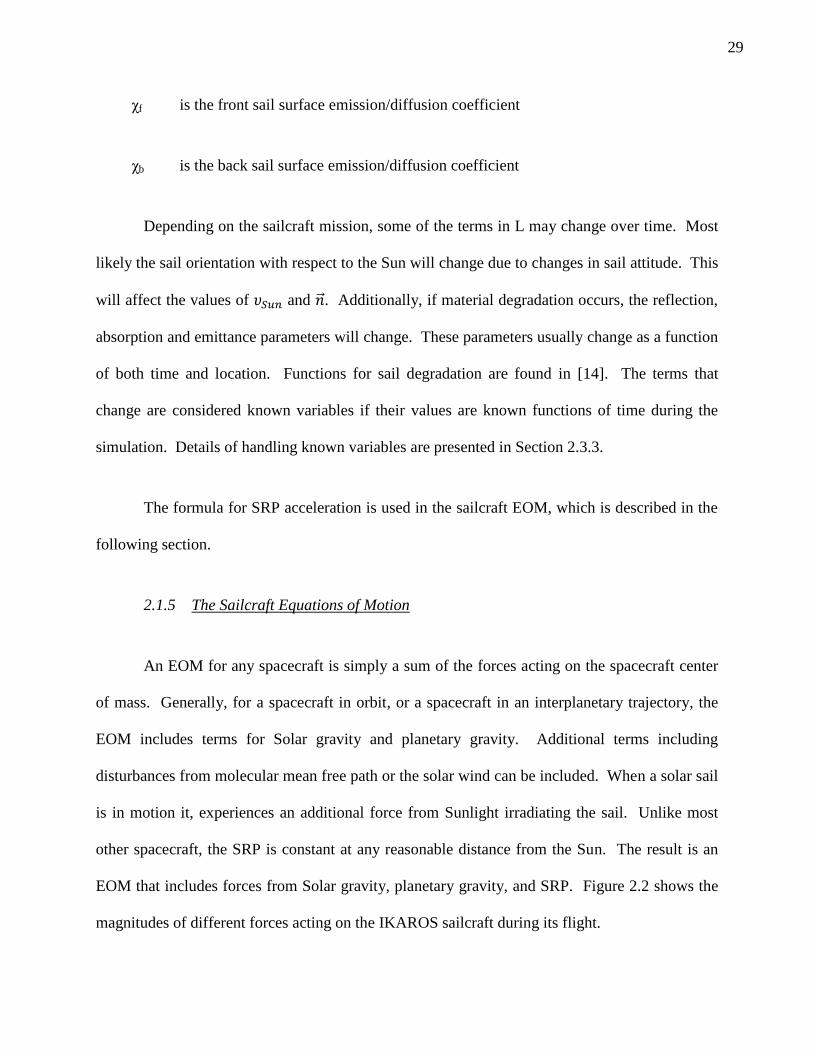
EOM that includes forces from Solar gravity, planetary gravity, and SRP. Figure 2.2 shows the

magnitudes of different forces acting on the IKAROS sailcraft during its flight.

30

Figure 2.2 Magnitudes of accelerations experienced by IKAROS

Like the gravity terms, the SRP is constantly changing as a function of the sailcraft

location, which further complicates the EOM. Mathematically speaking, the resulting sailcraft

EOM is a non-linear ordinary differential equation in time. Solving such an equation requires

numerical integration. This is where using the LSFEM is useful. Details of the LSFEM will be

saved for Section 2.3.

The sailcraft EOM describing motion influenced by SRP, Solar gravity, and planetary

gravity is shown in Equation (2.19) and Equation (2.20).

�̇� = 𝑉 (2.19)

31

�̇� = −𝜇𝑆𝑢𝑛𝑅

‖𝑅‖3+∑𝜇𝑝

𝑝

(−𝑅𝑝−𝑠

‖𝑅𝑝−𝑠‖3 +

𝑅𝑝

‖𝑅𝑝‖3) +

𝜇𝑆𝑢𝑛‖𝑅‖2

𝛯𝐿 (2.20)

where:

�̇� is the sailcraft acceleration vector in HIF

𝑉 is the sailcraft velocity vector in HIF

𝑅 is the sailcraft location vector in HIF

𝑅𝑝−𝑠 is the vector describing the distance from sailcraft to planet p

𝑅𝑝 is the location vector of planet p in HIF

𝐿 is the lightness vector

𝛯 is the transformation matrix from HOF to HIF

𝜇𝑆𝑢𝑛 is the Solar gravitation constant

𝜇𝑝 is the gravitation constant of planet p

For simplicity the velocity vector is left out to make the EOM take the form shown in

Equation (2.21).

32

�̈� = −𝜇𝑆𝑢𝑛𝑅

‖𝑅‖3+∑𝜇𝑝

𝑝

(−𝑅𝑝−𝑠

‖𝑅𝑝−𝑠‖3 +

𝑅𝑝

‖𝑅𝑝‖3) +


𝛯𝐿 (2.21)

where:

�̈� is the sailcraft acceleration vector in HIF, as the second time derivative of

location

The first RHS term quantifies the influence from solar gravity and the summed term provides the

influence of planetary gravity for any number of planets. The last term represents the

acceleration from SRP. A unique feature of the EOM is that despite including a thrust term, the

mass of the sailcraft remains constant, therefore, the sailcraft mass can be removed from the

EOM, resulting in a collection of acceleration terms.

2.2 Optimal Control

The LSFEM inherently has an optimization procedure that minimizes the squared

residuals of the sailcraft EOM. This optimization procedure will be used to maximize the thrust

of a sailcraft along a specific direction, which is controlled by sailcraft attitude adjustments. The

ability of the LSFEM to use high order polynomials for variable approximation functions means

the derivatives of the attitude angles are directly calculated within the LSFEM formulation. The

advantage of obtaining the derivatives is that they can be input directly into the spacecraft

angular rate equations to produce the torques required to perform the attitude changes.

An additional equation is solved alongside the equations of motion that adds the

33

capability of thrust optimization to the LSFEM simulation. This new equation is, in terms of

optimal control theory, acts as an objective function that solves for the optimum attitude angles.

2.2.1 Optimization

An optimization routine is found within the formulation of the finite element method.

Discussed in the finite element section are details of the conditions required to minimize the

residual functional. In particular, existence, necessary conditions, and sufficient conditions are

presented for determining a minimum of a functional [20][21]. This definition of determining

the minimum matches the necessary and sufficient conditions for determining a minimum using

optimal control theory [27][28][29][30]. In terms of optimal control, which include objective

functions and constraints, the equations of motion are the objective functions. Additional

objective functions can be included if more minimizations are desired.

The current LSFEM framework also has the ability to add optimal control to the solution

of the EOM. The LSFEM, like other finite element methods, inherently uses a minimization to

solve the system of differential equations. In the case of the LSFEM, the squared residual of the

system of equations is minimized. When the problem is setup appropriately, the squared residual

will be minimized to a value close to zero, thus producing a numerical solution. In terms of

optimal control, the squared residuals of the differential equations are objective functions.

Therefore, to add optimal control to the current LSFEM formulation, an additional objective

function can be added to the sailcraft EOM.

Optimal control gives the engineer the task of deciding what needs to be optimized and

what will drive to the optimization. A case has been formulated to maximize sailcraft thrust

34

along a given direction. The optimization will be controlled by the attitude of the sailcraft. The

state variables will be the location and velocity of the sailcraft, and the control variables will be

the sailcraft attitude angles. The optimization will determine the attitude change needed to

maximize the thrust.

Maximizing thrust in a specific direction is achieved by aligning the normal vector of the

sailcraft sail along the direction of maximum thrust. When this is achieved, the sail surface is

normal to the Sun, which maximizes the lightness vector, resulting in maximized thrust. An

objective function has been formulated to maximize thrust by changing the sailcraft attitude from

the current orientation. The following equation has been developed as the objective function for

performing the thrust optimization for a two-dimensional sailcraft trajectory.

𝛼 − 𝛼𝑓 − (𝛼𝑖 − 𝛼𝑓

1 + 𝑡5) = 0 (2.22)

where:

α is the sailcraft azimuth angle

αi is the initial azimuth angle

αf is the azimuth angle of the desired maximum thrust direction

t is time

35

This objective function is formulated to provide a smooth transition from the initial

sailcraft orientation to the orientation that provides the maximized thrust. Figure 2.3 shows

examples of the objective functions for three optimizations:

initial azimuth angle of 60° to azimuth angle of 30°



Figure 2.3 Objective Functions

The objective functions are added to the LSFEM formulation as an addition to the

sailcraft EOM. The implementation into the LSFEM is performed in asimilar manner to the

EOM with variable attitude angles.

36

2.2.2 Rate Equations

The spacecraft kinematic equations use the angular rates, angular accelerations, moments

of inertia, and products of inertia to determine the torque required to change the spacecraft

attitude. The optimization section shows that the attitude angles of the sailcraft can be solved

using the finite element framework. High order polynomial approximations provide the first and

second derivatives of the attitude angles, which fit directly into the attitude dynamics equations

for determining torque.

𝐼𝑥𝜔𝑥˙ + (𝐼𝑧 − 𝐼𝑦)𝜔𝑦𝜔𝑧 = 𝑇𝑥 (2.23)

𝐼𝑦𝜔𝑦˙ + (𝐼𝑥 − 𝐼𝑧)𝜔𝑥𝜔𝑧 = 𝑇𝑦 (2.24)

𝐼𝑧𝜔𝑧˙ + (𝐼𝑦 − 𝐼𝑥)𝜔𝑥𝜔𝑦 = 𝑇𝑧 (2.25)

where:

I is the sailcraft moment of inertia

𝜔 is the angular velocity

�̇� is the angular acceleration

T is the torque

37

x y z are the axes in the sailcraft HOF

Running either a variable attitude trajectory propagation or optimization, along with knowledge

of the sailcraft moments of inertia, provides the information required to determine the control

torques.

2.3 The Least Squares hpk Finite Element Method

The finite element method has made its mark in the field of structural analysis and is

showing popularity in the field of fluid dynamics. The general perception of FEM is that it is

used for structural mechanics and can be applied to fluid dynamics, but in reality the FEM is an

ODE and PDE solver. From the point of view of the FEM, the equations of continuum

mechanics used for structural and fluid analyses are simply PDEs. The independent variables

can be any number or combination of physical variables. When the EOM for sailcraft is

implemented in the FEM, it is seen as a one-dimensional non-linear ODE. When numerical

techniques are added, which is the case for the LSFEM method presented in this document, the

FEM becomes an unconditionally stable and accurate differential equation solver. Compared to

currently used numerical integration techniques for spacecraft, the LSFEM proves itself superior.

The following sections provide the details of the least squares hpk finite element method

used in this research.

2.3.1 Mathematical Overview

The finite element method takes differential equations and approximates their solutions

using three steps:

38

1. constructing a variation of a functional from the BVP or IVP

2. substituting polynomial approximations for the dependent variables

3. solving the resulting system of equations

The least squares process (LSP) is a method for creating the variation of a functional

using the differential equations. The least squares process for the FEM involves minimizing the

residuals of a functional based on the governing differential equation (GDE) being solved. To

understand the LSFEM consider the GDE to be a BVP in the form of Equation (2.26).

𝐴𝜑 − 𝑓 = 0 (2.26)

where:

A is the differential operator

φ is the dependent variable

f is the non-homogeneous term

The first step, as with all FEM, is replacing the dependent variable, φ, with an

approximation of the dependent variable, φn. Using the BVP, let a residual E be defined as

Equation (2.27) and, applying the least squares process, a residual functional I(φn) is defined by

Equation (2.28).

39

𝐴𝜑n − 𝑓 = 𝐸 (2.27)

𝐼(𝜑n) = (𝐸, 𝐸) = (𝐴𝜑n − 𝑓, 𝐴𝜑n − 𝑓) (2.28)

The meaning of the parenthesis in Equation (2.28) is defined in Equation (2.29) where Ω

is defined as the domain.

(𝑥, 𝑦) = ∫𝑥𝑦𝑑𝛺

𝛺 (2.29)

If 𝐼(𝜑𝑛) is differentiable by φn then the necessary condition for the extremum of 𝐼(𝜑𝑛) is

that the variation of 𝐼(𝜑𝑛) must be zero or 𝛿𝐼(𝜑𝑛) = 0. Equation (2.30) shows the variational

statement and how it affects the residuals.

𝛿𝐼(𝜑n) = (𝛿𝐸, 𝐸) + (𝐸, 𝛿𝐸) = 2(𝐸, 𝛿𝐸) = 0 (2.30)

A unique extremum principle means the formulation is variationally consistent (VC),

which leads to a mathematically and computationally sound formation. It also leads to a

minimization of 𝐼(𝜑𝑛) resulting in minimizing the residual of the GDE. The advantage of

minimizing the residual is obvious since the residual is the error resulting from substituting the

approximation functions into the GDE. When the algebraic system is formulated, the resulting

coefficient matrix will be symmetric and positive definite. For a unique extremum principle the

following formula in Equation (2.31) must hold true for the second variation of the residual.

40

𝛿2𝐼(𝜑n) = 2(𝛿𝐸, 𝛿𝐸) + 2(𝐸, 𝛿2𝐸) {> 0= 0< 0

} ∀𝑣 ∈ 𝑉𝑛 (2.31)

Reference [20] provides the mathematical framework for proving variational consistency

of linear operators. The result of the proof eliminates the second term of the residual's second

variation and shows the result is always positive. This is shown in Equation (2.32).

𝛿2𝐼(𝜑n) = 2(𝛿𝐸, 𝛿𝐸) > 0 (2.32)

For non-linear operators the above equation is used as a starting approximation. The first

variation of a BVP with a non-linear differential operator is treated as follows in Equation (2.33).

𝛿𝐸 = 𝛿(𝐴𝜑 − 𝑓) = 𝛿𝐴(𝜑𝑛) + 𝐴(𝛿𝜑𝑛) = 𝛿𝐴(𝜑𝑛) + 𝐴𝑣 = 0 (2.33)

Making the approximation from Equation (2.32) guarantees the variation of the residual

to have a unique extremum principle and results in variational consistency of the integral and a

unique solution. When the Newton's linear method is used along with the approximation from

Equation (2.32) the solution for φn is found iteratively and still maintains uniqueness. [20]

provides the mathematical proofs for the previous statements.

Newton's linear method, sometimes referred to as the Newton-Raphson method , provides

the necessary means for solving non-linear PDEs and ODEs using LSFEM while maintaining

41

variational consistency. Iterations are carried out based on the following formulation in

Equation (2.34) and Equation (2.35).

𝜑𝑛 = 𝜑𝑛0 + 𝛼𝛥𝜑𝑛 (2.34)

𝛥𝜑𝑛 = −1

2[𝛿2𝐼]𝜑𝑛0

−1𝑔(𝜑𝑛0) (2.35)

where:

𝜑𝑛0 is the initial or guessed solution

𝛼 is an iteration parameter

𝑔(𝜑𝑖) is described in Equation (2.36)

𝑔(𝜑𝑛) =1

2𝐼(𝜑𝑛) (2.36)

The parameter 𝛼 is determined using the inequality in Equation (2.37).

𝐼(𝜑𝑖) ≤ 𝐼(𝜑𝑖0) (2.37)

where:

42

i is the number of the current iteration

Iterations are repeated using the final values of the previous solution for the initial or

guessed solution of the current iteration. When a preset tolerance for either𝐼(𝜑𝑖) or 𝑔(𝜑𝑖) is

achieved, the iterations terminate and the numerical solution is determined.

Having a variationally consistent formulation provides numerous advantages. Variational

consistency means the coefficient matrices in the algebraic system formulated from the first

variation of the functional will always be symmetric and positive definite. These advantages

mean the resulting algebraic system is solvable mathematically and unconditionally stable

computationally.

Although this explanation of the LSFEM regards BVPs, the treatment of IVPs is no

different. In the case of an IVP like the sailcraft EOM, the LSFEM formulation is setup to solve

a one-dimensional, non-linear differential equation. The fact that the independent variable is

time and not a spacial variable does not have any effect. However, an IVP has the ability to

numerically solve the GDE through time by performing calculations one element at a time. The

next section describes the mesh and time domain used in the computations and includes an

explanation of calculating solutions element-by-element.

2.3.2 Element Mesh and Time Steps

At least one element is needed to run an FEM simulation. When dealing with a domain

consisting of only time, this can be advantageous. This is from the nature of the evolution of all

physical processes. Therefore, only a single element is needed to calculate the solution of a

43

differential equation and the solution will not differ from a simulation that uses multiple

elements.

The setup for a time domain that requires multiple elements can be split into time steps

that involve a single element. Initial conditions of the first element are used to calculate the

solution at the element's end node, which then become the initial conditions for the next element.

Computationally, there's generally less code involved in a single element formulation, but a time

stepping loop is required when multiple elements are needed.

The element size must have the appropriate resolution to capture changes in the solution

variables. If a time step is too large it may not capture changes in the variables that occur

between the end nodes of the element. This LSFEM formulation is able to capture these

changes, however, care needs to be taken to make sure the element size is still appropriate.

A distinct advantage of this formulation of the FEM is its ability to provide a unique

solution for an overdetermined system of equations. In Section 2.5.4, the reward of this

advantage will be described.

2.3.3 Variable Approximations

A distinct advantage of this LSFEM framework is the high order global differentiability.

This is described in this section as part of the description of the variable approximations. In most

finite element formulations, the approximations of the dependent variables are based on linear or

quadratic shape functions that are multiplied by the element's degrees of freedom. This is the

same technique for the present formulation, however, the shape functions are more complex

44

allowing the approximation functions to reach high-order polynomial shape functions and global

differentiability.

Consider 𝑁(𝑡)𝑖 the local approximation functions where 𝛿𝑖𝑒 is the nodal degree of

freedom vector and 𝑥ℎ𝑒 is the approximation of x over an element e. An approximation of 𝑥ℎ

𝑒 is

presented in Equation (2.38):

𝑥ℎ𝑒 =∑𝑁

𝑛

𝑖=1

(𝑡)𝑖𝑥𝑖𝑒 = [𝑁]{𝑥𝑒} (2.38)

where:

𝑁(𝑡)𝑖 is the vector of the local approximation functions

𝛿𝑖𝑒 is the nodal degree of freedom vector

𝑥ℎ𝑒 is the approximation of x over an element e

Similarly, Equation (2.39) shows the formulation for 𝑦ℎ𝑒.

𝑦ℎ𝑒 =∑𝑁

𝑛

𝑖=1

(𝑡)𝑖𝑦𝑖𝑒 = [𝑁]{𝑦𝑒} (2.39)

The vectors of the degrees of freedom, {𝑥𝑒} and {𝑦𝑒}, depend of the type of approximation

function [𝑁].

45

Before the approximation functions can be described the natural coordinate space will be

introduced. The EOMs for sailcraft are ODEs with variables and derivatives with respect to

time. During the simulations time can be input in days, months, or years, however, the LSFEM

sees time in the natural coordinate system. The domain for each element in time is mapped into

the natural coordinate system in a manner that shrinks or expands the element domain to [-1,1].

This is done using a linear interpolation that uses the end nodes of the one-dimensional time

elements.

The interpolation for mapping points from physical coordinates to natural coordinates is

defined by Equation (2.40).

𝑡(𝜉) = (1 − 𝜉

2) 𝑡1 + (

1 + 𝜉

2) 𝑡2 (2.40)

where:

𝑡(𝜉) is definition of the mapping from physical to natural coordinate space

𝜉 is the independent variable in the natural coordinate space

𝑡1 is the value of t at element node 1

𝑡2 is the value of t at element node 2

Plugging in the node values of t into the Equation (2.40) and varying the value of 𝜉 can

demonstrate how the interpolation works. Notice how the two lines sum to unity across the

46

domain of the element, this is the case for all types of interpolating functions.

Like the time domain discussed previously, the dependent variables are required to be

mapped to the natural coordinate space. As an example, Equation (2.41) shows the

approximation of x over an element e in the natural coordinate space.

𝑥𝑒 = (1 − 𝜉

2) 𝑥1

𝑒 + (1 + 𝜉

2) 𝑥2

𝑒 (2.41)

y follows the same formulation in Equation (2.42).

𝑦𝑒 = (1 − 𝜉

2) 𝑦1

𝑒 + (1 + 𝜉

2) 𝑦2

𝑒 (2.42)

Equation (2.41) can be rearranged to match the formula in Equation (2.38) using the

formulations below.

[𝑁] = [(1 − 𝜉

2) (

1 + 𝜉

2)] (2.43)

{𝛿𝑒} = [𝑥1𝑒 𝑥2

𝑒]𝑇 (2.44)

𝑥𝑒 = [𝑁]{𝛿𝑒} (2.45)

Equation (2.41) and Equation (2.42) are linear interpolation functions and represent the

47

lowest and least accurate level that the LSFEM has to offer. Interpolation equations range from

quadratic functions to high order polynomials exceeding 10th

order. Mathematical descriptions

of these functions are left to [20]. Important to the research presented in this document is the

third-order polynomial interpolation. [20] shows that beginning at the third order function, the

degrees of freedom include derivatives of the solution variables. This means that for the

approximation shown in Equation (2.46), the resulting degrees of freedom are in the vector

shown in Equation (2.47).

𝑥ℎ𝑒 = [𝑁]{𝑥𝑒} (2.46)

{𝑥𝑒} =

{

𝑥1𝑒

𝜕𝑥1𝑒

𝜕𝑡𝑥2𝑒

𝜕𝑥2𝑒

𝜕𝑡 }

(2.47)

The y approximation follows the same style. Jumping ahead to consider the EOM, the above

formulation provides simultaneous solutions for location and velocity.

Starting at a third-order polynomial approximation, the LSFEM formulation provides

global differentiability up to first order. Approximation functions extend further to provide

higher orders of global differentiability. This means, in terms of the EOM, solutions for

acceleration are solved alongside the location and velocity. The addition of these degrees of

freedom allows for more information to be input into the EOM solver. This results in a more

accurate solution with additional outputs. In terms of computations, high order global

48

differentiation results in higher accuracy.

Extending the degrees of freedom to include first and second order derivatives brings the

solution closer to the true physical solution. The solution of the LSFEM formulation provides a

continuous, numerical solution for the degrees of freedom. For sailcraft, degrees of freedom

include vector of location, velocity, and acceleration, which, considering the physics of the

trajectory, are all continuous functions. Derivatives describe the physics of the sailcraft

trajectory, therefore, it is extremely important to achieve a solution with continuous derivatives.

Often, spacecraft trajectory propagation methods only provide continuous solutions for location

and velocity, which leaves acceleration to be calculated by differencing methods. Adding

additional calculations introduces new and unknown error values. Differencing methods can

provide adequate solutions for acceleration across most of the trajectory time domain, but they

fall short at the boundaries where the data is limited.

2.4 Implementing the Equations of Motion

This section presents the LSFEM formulation for the sailcraft EOM using the details of

the previous section. To clearly show how the EOM is implemented, the 2-D EOM with Solar

gravity and SRP contributions will be described in detail. Additional formulations will be

presented without description but will follow the same methodology.

2.4.1 One-Dimensional SRP Thrust

The one-dimensional equation, shown below, calculates the acceleration from SRP for a

flat sail surface normal to the Sun.

49

𝑑2𝑅

𝑑𝑡2=1

𝑅2𝑘 (2.48)

The constant k is defined below:

𝑘 =𝑊𝐸

𝑐

𝑆

𝑚

𝑡𝑦𝑟2

𝐿1𝐴𝑈(1 + 𝛾𝐵(𝑓)) (2.49)

The residual is formed by rearranging the thrust equation and substituting the variable

approximation:

𝐸 =𝑑2𝑅ℎ

𝑒

𝑑𝑡2−

1

(𝑅ℎ𝑒)2

𝑘 (2.50)

where:

𝑅ℎ𝑒 = [𝑁]{𝑅𝑒} is the distance of the sailcraft from the Sun in AU

The variation of the residual is:

𝛿𝐸 = (𝑅ℎ𝑒)2

𝑑2𝑁

𝑑𝑡2+ 2𝑅ℎ

𝑒𝑑2𝑅ℎ

𝑒

𝑑𝑡2𝑁 − 𝑘 (2.51)

Depending on the order of the approximation space, the vector {𝑅𝑒} will include the distance

between the sailcraft and the Sun and time derivatives of the distance. For a second order

50

variable approximation, the vector will include sailcraft distance, velocity, and acceleration

relative to the Sun.

2.4.2 Two-Dimensional EOM without Planetary Gravity

The two-dimensional EOM is a truncated version of Equation (2.21) due to the removal

of the planetary gravity term. Equation (2.52) shows the vector formulation of the EOM.


‖𝑅‖3+𝜇𝑆𝑢𝑛‖𝑅‖2

𝛯𝐿 (2.52)

The vectors represent only x and y terms. Separating the x and y terms results in Equation (2.53)

and Equation (2.54).

𝑅3�̈� = 𝜇(𝜌𝑥 − 𝜏𝑦 − 𝑥) (2.53)

𝑅3�̈� = 𝜇(𝜌𝑦 + 𝜏𝑥 − 𝑦) (2.54)

The residual functions for the LSFEM are constructed from the above equations to form

Equation (2.55) and Equation (2.56).

𝐸1 = 𝑅3�̈� − 𝜇(𝜌𝑥 − 𝜏𝑦 − 𝑥) (2.55)

𝐸2 = 𝑅3�̈� − 𝜇(𝜌𝑦 + 𝜏𝑥 − 𝑦) (2.56)

51

where:

𝑅 = √(𝑥2 + 𝑦2) is the distance between the sailcraft and the Sun

𝜌 is the x-component of the lightness vector

𝜏 is the y-component of the lightness vector

Consider the local approximation functions, 𝑁(𝑡)𝑖, the nodal degrees of freedom, 𝛿𝑖𝑒, and

the approximation of x over an element e, 𝑥ℎ𝑒. Applying the local approximations changes the

residuals to the following form.

𝐸1𝑒 = ((𝑥ℎ

𝑒)2 + (𝑦ℎ𝑒)2)(3 2⁄ ) 𝜕𝑥ℎ

𝑒

𝜕𝑡− 𝜇(𝜌𝑥ℎ

𝑒 − 𝜏𝑦ℎ𝑒 − 𝑥ℎ

𝑒) (2.57)


𝑒)2 + (𝑦ℎ𝑒)2)(3 2⁄ ) 𝜕𝑦ℎ

𝑒

𝜕𝑡− 𝜇(𝜌𝑦ℎ

𝑒 + 𝜏𝑥ℎ𝑒 − 𝑦ℎ

𝑒) (2.58)

From the previous section, the local approximation functions of the sailcraft position

components are Equation (2.59) and Equation (2.60).

𝑥ℎ𝑒 = [𝑁]{𝑥𝑒} (2.59)

𝑦ℎ𝑒 = [𝑁]{𝑦𝑒} (2.60)

For first order global differentiability, the degree of freedom vectors take the following

52

forms.

{𝑥𝑒} =

{

𝑥1𝑒

𝜕𝑥1𝑒

𝜕𝑡𝑥2𝑒

𝜕𝑥2𝑒

𝜕𝑡 }

(2.61)

{𝑦𝑒} =

{

𝑦1𝑒

𝜕𝑦1𝑒

𝜕𝑡𝑦2𝑒

𝜕𝑦2𝑒

𝜕𝑡 }

(2.62)

The element degrees of freedom take the following form:

𝑥1𝑒

𝑑𝑥1𝑒

𝑑𝑡

𝑦1𝑒

𝑑𝑦1𝑒

𝑑𝑡

𝑥2𝑒

𝑑𝑥2𝑒

𝑑𝑡

𝑦2𝑒

𝑑𝑦2𝑒

𝑑𝑡

𝑥2𝑒

𝑑𝑥2𝑒

𝑑𝑡

𝑦2𝑒

𝑑𝑦2𝑒

𝑑𝑡

𝑥3𝑒

𝑑𝑥3𝑒

𝑑𝑡

𝑦3𝑒

𝑑𝑦3𝑒

𝑑𝑡

Taking the derivatives of the residuals with respect to the degree of freedom vectors

provides the variations of the residuals in Equation (2.63) and Equation (2.64).

1 2 2 3

element

1

element

2 node node node node

53

{𝛿𝐸1𝑒} =

{

3𝑅𝑥

𝜕2𝑥ℎ𝑒

𝜕𝑡2{𝑁} + 𝑅3 {

𝜕2𝑁

𝜕𝑡2} − 𝜇𝜌{𝑁} + 𝜇{𝑁}

3𝑅𝑦𝜕2𝑥ℎ

𝑒

𝜕𝑡2{𝑁} + 𝜇𝜏{𝑁}

}

(2.63)

{𝛿𝐸2𝑒} =

{

3𝑅𝑥

𝜕2𝑦ℎ𝑒

𝜕𝑡2{𝑁} − 𝜇𝜏{𝑁}

3𝑅𝑦𝜕2𝑦ℎ

𝑒

𝜕𝑡2{𝑁} + 𝑅3 {

𝜕2𝑁

𝜕𝑡2} − 𝜇𝜌{𝑁} + 𝜇{𝑁}

}

(2.64)

With the above equations the 𝐾 matrix and 𝑔 vector can be calculated using an initial

guess for the non-linear terms.

2.4.3 Two-Dimensional EOM with Variable Lightness Vector

The vector form of the two-dimensional EOM with a variable lightness vector takes the

same form as the previous EOM:

�̈� = −𝜇Sun𝑅

‖𝑅‖3+𝜇Sun‖𝑅‖2

ΞL (2.65)

where the two-dimensional vector variables are:

𝑅 = [𝑥 𝑦]𝑇 (2.66)

54

𝐿 = [𝜌 𝜏]𝑇 (2.67)

Separated out of vector form, the system of equations becomes:

𝑅3�̈� − 𝜇(𝜌𝑥 − 𝜏𝑦 − 𝑥) = 0 (2.68)

𝑅3�̈� − 𝜇(𝜌𝑥 + 𝜏𝑦 − 𝑦) = 0 (2.69)

At this step it is now possible to start the implementation into the LSFEM. The degrees

of freedom at each node contain variables of sailcraft location, velocity, and the lightness vector

components. When the lightness vector is a known variable, it can utilize first order global

differentiability. If the lightness vector is an unknown variable it cannot utilize global

differentiability, as this will introduce too many unknowns into the LSFEM solution. For

unknown lightness vectors, the components can be solved accurately using high order

polynomial approximation functions.

The residual functions for the variable lightness vector formulation are shown below:


𝑒)2 + (𝑦ℎ𝑒)2)(3 2⁄ ) 𝜕𝑥ℎ

𝑒

𝜕𝑡− 𝜇(𝜌ℎ

𝑒𝑥ℎ𝑒 − 𝜏ℎ

𝑒𝑦ℎ𝑒 − 𝑥ℎ

𝑒) (2.70)

55


𝑒)2 + (𝑦ℎ𝑒)2)(3 2⁄ ) 𝜕𝑦ℎ

𝑒

𝜕𝑡− 𝜇(𝜌ℎ

𝑒𝑦ℎ𝑒 + 𝜏ℎ

𝑒𝑥ℎ𝑒 − 𝑦ℎ

𝑒) (2.71)

The residuals are similar to the two-dimensional EOM, except that these contain approximations

for the lightness vector components. Two more rows are added to the variations of the residuals

due to the addition of the two lightness vector variables.

{𝛿𝐸1𝑒} =

{

3𝑅𝑥

𝜕2𝑥ℎ𝑒

𝜕𝑡2{𝑁} + 𝑅3 {

𝜕2𝑁

𝜕𝑡2} − 𝜇𝜌{𝑁} + 𝜇{𝑁}


𝑒

𝜕𝑡2{𝑁} + 𝜇𝜏{𝑁}

−𝜇𝑥ℎ𝑒{𝑁}

𝜇𝑦ℎ𝑒{𝑁} }

(2.72)

{𝛿𝐸2𝑒} =

{

3𝑅𝑥

𝜕2𝑦ℎ𝑒

𝜕𝑡2{𝑁} − 𝜇𝜏{𝑁}


𝑒

𝜕𝑡2{𝑁} + 𝑅3 {

𝜕2𝑁

𝜕𝑡2} − 𝜇𝜌{𝑁} + 𝜇{𝑁}

−𝜇𝑦ℎ𝑒{𝑁}

−𝜇𝑥ℎ𝑒{𝑁} }

(2.73)

The variable approximations are defined as:

𝑥ℎ𝑒 = [𝑁]{𝑥𝑒} (2.74)

𝑦ℎ𝑒 = [𝑁]{𝑦𝑒} (2.75)

56

𝜌ℎ𝑒 = [𝑁]{𝜌𝑒} (2.76)

𝜏ℎ𝑒 = [𝑁]{𝜏𝑒} (2.77)

Presented below are the element degrees of freedom for a variable lightness vector.

𝑥1𝑒

𝑑𝑥1𝑒

𝑑𝑡

𝑦1𝑒

𝑑𝑦1𝑒

𝑑𝑡

𝜌1𝑒

𝑑𝜌1𝑒

𝑑𝑡

𝜏1𝑒

𝑑𝜏1𝑒

𝑑𝑡

𝑥2𝑒

𝑑𝑥2𝑒

𝑑𝑡

𝑦2𝑒

𝑑𝑦2𝑒

𝑑𝑡

𝜌2𝑒

𝑑𝜌2𝑒

𝑑𝑡

𝜏2𝑒

𝑑𝜏2𝑒

𝑑𝑡

𝑥2𝑒

𝑑𝑥2𝑒

𝑑𝑡

𝑦2𝑒

𝑑𝑦2𝑒

𝑑𝑡

𝜌2𝑒

𝑑𝜌2𝑒

𝑑𝑡

𝜏2𝑒

𝑑𝜏2𝑒

𝑑𝑡

𝑥3𝑒

𝑑𝑥3𝑒

𝑑𝑡

𝑦3𝑒

𝑑𝑦3𝑒

𝑑𝑡

𝜌3𝑒

𝑑𝜌3𝑒

𝑑𝑡

𝜏3𝑒

𝑑𝜏3𝑒

𝑑𝑡

2.4.4 Two-Dimensional EOM with Variable Attitude

The EOM with variable attitude takes the same vector form as the previous two EOM

formulations. The variables, however, are now location and the sailcraft azimuth angle. Starting

with the two-dimensional EOM:

�̈� = −𝜇Sun𝑅

‖𝑅‖3+𝜇Sun‖𝑅‖2

ΞL (2.78)

1 2 2 3

element

1

element

2 node node node node

57

which then takes the form:

𝑅3�̈� − 𝜇(𝜌𝑥 − 𝜏𝑦 − 𝑥) = 0 (2.79)

𝑅3�̈� − 𝜇(𝜌𝑥 + 𝜏𝑦 − 𝑦) = 0 (2.80)

The azimuth angle is found within the radial and tangential components of the lightness vector.

For three-dimensional formulations, the azimuth and elevation angles are within all three

components of the lightness vector. The lightness vector components for the two-dimensional

EOM are presented below in terms of 𝛼:

ρ =

1

2

σcrσcos(α)[(2ℜscos(α) + χfℜdsin(π 2⁄ + 0.675α) + Afκsail)cos(−α)

+(Af +ℜd) − (χfℜdcos(π 2⁄ + 0.675α))sin(α)]

(2.81)

𝜏 =

1

2

𝜎𝑐𝑟𝜎𝑐𝑜𝑠(𝛼)[(2ℜ𝑠𝑐𝑜𝑠(𝛼) + 𝜒𝑓ℜ𝑑𝑠𝑖𝑛(𝜋 2⁄ + 0.675𝛼) + 𝐴𝑓𝜅𝑠𝑎𝑖𝑙)𝑠𝑖𝑛(−𝛼)

− (𝜒𝑓ℜ𝑑𝑐𝑜𝑠(𝜋 2⁄ + 0.675𝛼)) 𝑐𝑜𝑠(𝛼)] (2.82)

The residuals are presented below:


𝑒)2 + (𝑦ℎ𝑒)2)(3 2⁄ ) 𝜕𝑥ℎ

𝑒

𝜕𝑡− 𝜇(𝜌𝑥ℎ


𝑒) (2.83)


𝑒)2 + (𝑦ℎ𝑒)2)(3 2⁄ ) 𝜕𝑦ℎ

𝑒

𝜕𝑡− 𝜇(𝜌𝑦ℎ


𝑒) (2.84)

58

The variations of the residuals are presented in the following two equations:

{𝛿𝐸1𝑒} =

{

3𝑅𝑥

𝜕2𝑥ℎ𝑒

𝜕𝑡2{𝑁} + 𝑅3 {

𝜕2𝑁

𝜕𝑡2} − 𝜇𝜌{𝑁} + 𝜇{𝑁}


𝑒

𝜕𝑡2{𝑁} + 𝜇𝜏{𝑁}

−𝜇𝑥𝜕𝜌

𝜕{𝛼ℎ𝑒}+ 𝜇𝑦

𝜕𝜏

𝜕{𝛼ℎ𝑒} }

(2.85)

{𝛿𝐸2𝑒} =

{

3𝑅𝑥

𝜕2𝑦ℎ𝑒

𝜕𝑡2{𝑁} − 𝜇𝜏{𝑁}


𝑒

𝜕𝑡2{𝑁} + 𝑅3 {

𝜕2𝑁

𝜕𝑡2} − 𝜇𝜌{𝑁} + 𝜇{𝑁}

−𝜇𝑥𝜕𝜌

𝜕{𝛼ℎ𝑒}− 𝜇𝑦

𝜕𝜏

𝜕{𝛼ℎ𝑒} }

(2.86)

where:

𝑅 = √(𝑥2 + 𝑦2)

The derivatives of the lightness vector components with respect to the azimuth angle are

presented in the following two equations:

59

𝜕𝜌

𝜕{𝛼ℎ𝑒}=

−𝜎𝑐𝑟2𝜎

𝑠𝑖𝑛(𝛼ℎ𝑒)

[(2ℜ𝑠𝑐𝑜𝑠(𝛼ℎ𝑒) + 𝜒𝑓ℜ𝑑𝑠𝑖𝑛(𝜋 2⁄ + 0.675𝛼ℎ

𝑒) + 𝐴𝑓𝜅𝑠𝑎𝑖𝑙)𝑐𝑜𝑠(−𝛼ℎ𝑒) +

(𝐴𝑓 +ℜ𝑑) − (𝜒𝑓ℜ𝑑𝑐𝑜𝑠(𝜋 2⁄ + 0.675𝛼ℎ𝑒)) 𝑠𝑖𝑛(𝛼ℎ

𝑒)] +

𝜎𝑐𝑟2𝜎

𝑐𝑜𝑠(𝛼ℎ𝑒)

[−𝑠𝑖𝑛(−𝛼ℎ𝑒)(2ℜ𝑠𝑐𝑜𝑠(𝛼ℎ

𝑒) + 𝜒𝑓ℜ𝑑𝑠𝑖𝑛(𝜋 2⁄ + 0.675𝛼ℎ𝑒) + 𝐴𝑓𝜅𝑠𝑎𝑖𝑙) +]

𝑐𝑜𝑠(−𝛼ℎ𝑒)(−2ℜ𝑠𝑠𝑖𝑛(𝛼ℎ

𝑒) + 0.675𝜒𝑓ℜ𝑑𝑐𝑜𝑠(𝜋 2⁄ + 0.675𝛼ℎ𝑒)) −

𝑐𝑜𝑠(𝛼ℎ𝑒)(2ℜ𝑠𝑐𝑜𝑠(𝛼ℎ

𝑒) + 𝜒𝑓ℜ𝑑𝑠𝑖𝑛(𝜋 2⁄ + 0.675𝛼ℎ𝑒) + 𝐴𝑓𝜅𝑠𝑎𝑖𝑙) +

𝑠𝑖𝑛(𝛼ℎ𝑒)(0.675𝜒𝑓ℜ𝑑𝑠𝑖𝑛(𝜋 2⁄ + 0.675𝛼ℎ

𝑒))

(2.87)

𝜕𝜏

𝜕{𝛼ℎ𝑒}=

−𝜎𝑐𝑟2𝜎

𝑠𝑖𝑛(𝛼ℎ𝑒)

[(2ℜ𝑠𝑐𝑜𝑠(𝛼ℎ𝑒) + 𝜒𝑓ℜ𝑑𝑠𝑖𝑛(𝜋 2⁄ + 0.675𝛼ℎ

𝑒) + 𝐴𝑓𝜅𝑠𝑎𝑖𝑙)𝑐𝑜𝑠(−𝛼ℎ𝑒) +

(𝐴𝑓 +ℜ𝑑) − (𝜒𝑓ℜ𝑑𝑐𝑜𝑠(𝜋 2⁄ + 0.675𝛼ℎ𝑒)) 𝑠𝑖𝑛(𝛼ℎ

𝑒)] +

𝜎𝑐𝑟2𝜎

𝑐𝑜𝑠(𝛼ℎ𝑒)

[𝑐𝑜𝑠(−𝛼ℎ𝑒)(2ℜ𝑠𝑐𝑜𝑠(𝛼ℎ

𝑒) + 𝜒𝑓ℜ𝑑𝑠𝑖𝑛(𝜋 2⁄ + 0.675𝛼ℎ𝑒) + 𝐴𝑓𝜅𝑠𝑎𝑖𝑙) +]

𝑠𝑖𝑛(−𝛼ℎ𝑒)(−2ℜ𝑠𝑠𝑖𝑛(𝛼ℎ

𝑒) + 0.675𝜒𝑓ℜ𝑑𝑐𝑜𝑠(𝜋 2⁄ + 0.675𝛼ℎ𝑒)) +

𝑠𝑖𝑛(𝛼ℎ𝑒)(2ℜ𝑠𝑐𝑜𝑠(𝛼ℎ

𝑒) + 𝜒𝑓ℜ𝑑𝑠𝑖𝑛(𝜋 2⁄ + 0.675𝛼ℎ𝑒) + 𝐴𝑓𝜅𝑠𝑎𝑖𝑙) +

𝑐𝑜𝑠(𝛼ℎ𝑒)(0.675𝜒𝑓ℜ𝑑𝑠𝑖𝑛(𝜋 2⁄ + 0.675𝛼ℎ

𝑒))

(1)

(2.88)

The variable approximations are defined as:

𝑥ℎ𝑒 = [𝑁]{𝑥𝑒} (2.89)

𝑦ℎ𝑒 = [𝑁]{𝑦𝑒} (2.90)

60

𝛼ℎ𝑒 = [𝑁]{𝛼𝑒} (2.91)

The degrees of freedom for each node of an element e are:

𝛿𝑒 = [𝑥ℎ𝑒 𝑑𝑥ℎ

𝑒

𝑑𝑡 𝑦ℎ

𝑒 𝑑𝑦ℎ

𝑒

𝑑𝑡 𝛼ℎ

𝑒 𝑑𝛼ℎ

𝑒

𝑑𝑡]𝑇 (2.92)

2.4.5 Two-Dimensional EOM with Planetary Gravity

The EOM is repeated below in Equation (2.93):


‖𝑅‖3+∑𝜇𝑝

𝑝

(−𝑅𝑝−𝑠

‖𝑅𝑝−𝑠‖3 +

𝑅𝑝

‖𝑅𝑝‖3) +


𝛯𝐿 (2.93)

The component functions are shown in Equation (2.94) and Equation (2.95) with accompanying

formulas in the equations below.

𝑅3�̈� − (𝜌𝑥 − 𝜏𝑦 − 𝑥) +∑𝜇𝑝𝐷𝑝3(𝑥 − 𝑥𝑝)

𝑛

𝑝=1

= 0 (2.94)

𝑅3�̈� − (𝜌𝑦 + 𝜏𝑥 − 𝑦) +∑𝜇𝑝𝐷𝑝3(𝑦 − 𝑦𝑝)

𝑛

𝑝=1

= 0 (2.95)

61

𝑅 = √𝑥2 + 𝑦2 (2.96)

𝑅𝑝 = √(𝑥 − 𝑥𝑝)2+ (𝑦 − 𝑦𝑝)

2 (2.97)

𝐷 = 𝑅 𝑅𝑝⁄ (2.98)

where:

𝜇𝑝 is the gravitational constant for planet p

𝑥𝑝 is the x-component of the location of planet p

𝑦𝑝 is the y-component of the location of planet p

𝑛 is the total number of planets in the simulation



The residuals with the variable approximations are presented in Equation (2.99) and

Equation (2.100), they are found in the same manner as the previous EOM, with additional

formulations in Equation (2.101) and Equation (2.102).

62

𝐸1𝑒 = 𝑅3

𝜕2𝑥ℎ𝑒

𝜕𝑡2− 𝜇(𝜌𝑥ℎ


𝑒) + 𝑝𝑥 (2.99)

𝐸2𝑒 = 𝑅3

𝜕2𝑦ℎ𝑒

𝜕𝑡2− 𝜇(𝜌𝑦ℎ


𝑒) + 𝑝𝑦 (2.100)

𝑝𝑥 =∑𝜇𝑝𝐷𝑝3(𝑥ℎ

𝑒 − (𝑥ℎ𝑒)𝑝)

𝑛

𝑝=1

(2.101)

𝑝𝑦 =∑𝜇𝑝𝐷𝑝3(𝑦ℎ

𝑒 − (𝑦ℎ𝑒)𝑝)

𝑛

𝑝=1

(2.102)

The variations of the residuals are presented in Equation (2.103) and Equation (2.104).

{𝛿𝐸1𝑒} =

{

3𝑅𝑥

𝜕2𝑥

𝜕𝑡2{𝑁} + 𝑅3 {

𝜕2𝑁

𝜕𝑡2} − 𝜇𝜌{𝑁} + 𝜇{𝑁} +

𝜕𝑝𝑥𝜕{𝑥}

3𝑅𝑦𝜕2𝑥

𝜕𝑡2{𝑁} + 𝜇𝜏{𝑁} +

𝜕𝑝𝑥𝜕{𝑦}

𝜕𝑝𝑥𝜕{𝑥1}

𝜕𝑝𝑥𝜕{𝑦1}

𝜕𝑝𝑥𝜕{𝑥2}

𝜕𝑝𝑥𝜕{𝑦2} }

(2.103)

63

{𝛿𝐸2𝑒} =

{

3𝑅𝑥

𝜕2𝑦

𝜕𝑡2{𝑁} − 𝜇𝜏{𝑁} +

𝜕𝑝𝑦

𝜕{𝑥}

3𝑅𝑦𝜕2𝑦

𝜕𝑡2{𝑁} + 𝑅3 {

𝜕2𝑁

𝜕𝑡2} − 𝜇𝜌{𝑁} + 𝜇{𝑁} +

𝜕𝑝𝑦

𝜕{𝑦}

𝜕𝑝𝑦

𝜕{𝑥1}

𝜕𝑝𝑦

𝜕{𝑦1}

𝜕𝑝𝑦

𝜕{𝑥2}

𝜕𝑝𝑦

𝜕{𝑦2} }

(2.104)

The derivatives in the above equations are displayed in the following equations:

𝜕𝑝𝑥𝜕{𝑥}

= ∑𝜇𝑝 [3𝐿𝑝2 (

𝑥

𝑅 ∙ 𝑅𝑝−𝑅

𝑅𝑝3 (𝑥 − 𝑥𝑝)) (𝑥 − 𝑥𝑝) + 𝐿𝑝

3 ]

𝑛

𝑝=1

{𝑁} (2.105)

𝜕𝑝𝑥𝜕{𝑦}

= ∑𝜇𝑝 [3𝐿𝑝2 (

𝑦


𝑅𝑝3 (𝑦 − 𝑦𝑝)) (𝑥 − 𝑥𝑝)]

𝑛

𝑝=1

{𝑁} (2.106)

𝜕𝑝𝑥

𝜕{𝑥𝑝}= 𝜇𝑝 [3𝐿𝑝

2𝑅

𝑅𝑝3 (𝑥 − 𝑥𝑝)

2− 𝐿𝑝

3 ] {𝑁} (2.107)

𝜕𝑝𝑥

𝜕{𝑦𝑝}= 𝜇𝑝 [3𝐿𝑝

2𝑅

𝑅𝑝3 (𝑦 − 𝑦𝑝)(𝑥 − 𝑥𝑝)] {𝑁} (2.108)

64

𝜕𝑝𝑦

𝜕{𝑥}= ∑𝜇𝑝 [3𝐿𝑝

2 (𝑥


𝑅𝑝3 (𝑥 − 𝑥𝑝)) (𝑦 − 𝑦𝑝) + 𝐿𝑝

3 ]

𝑛

𝑝=1

{𝑁} (2.109)

𝜕𝑝𝑦

𝜕{𝑦}= ∑𝜇𝑝 [3𝐿𝑝

2 (𝑦


𝑅𝑝3 (𝑦 − 𝑦𝑝)) (𝑦 − 𝑦𝑝)]

𝑛

𝑝=1

{𝑁} (2.110)

𝜕𝑝𝑦

𝜕{𝑥𝑝}= 𝜇𝑝 [3𝐿𝑝

2𝑅

𝑅𝑝3 (𝑥 − 𝑥𝑝)(𝑦 − 𝑦𝑝)] {𝑁} (2.111)

𝜕𝑝𝑦

𝜕{𝑦𝑝}= 𝜇𝑝 [3𝐿𝑝

2𝑅

𝑅𝑝3 (𝑦 − 𝑦𝑝)

2− 𝐿𝑝

3 ] {𝑁} (2.112)

The degree of freedom vector follows similarly to the previous EOM with the addition of the

planet variables. Equation (2.113) shows the DOF vector for this formulation.

𝛿𝑒 = [𝑥ℎ𝑒 𝑑𝑥ℎ

𝑒

𝑑𝑡 𝑦ℎ

𝑒 𝑑𝑦ℎ

𝑒

𝑑𝑡 (𝑥ℎ

𝑒)𝑝 (𝑑𝑥ℎ

𝑒

𝑑𝑡)𝑝

(𝑦ℎ𝑒)𝑝 (

𝑑𝑦ℎ𝑒

𝑑𝑡)𝑝

]

𝑇

(2.113)

For simulations with more planets, additional degrees of freedom are included for

planetary location and velocity.

2.4.6 3D EOM without Planetary Gravity

The sailcraft equation of motion with SRP and Solar gravity contributions is presented

below:

65


‖𝑅‖3+𝜇𝑆𝑢𝑛‖𝑅‖2

𝛯𝐿 (2.114)

The following equations present the individual components of the EOM:

𝑅3𝐴�̈� − 𝜇𝐴(𝜌 − 1)𝑥 + 𝜇𝜏[𝑦(�̇�𝑥 − �̇�𝑦) + 𝑧(�̇�𝑥 − �̇�𝑧)] − 𝜇𝑅𝜂(�̇�𝑦 − �̇�𝑧) = 0 (2.115)

𝑅3𝐴�̈� − 𝜇𝐴(𝜌 − 1)𝑦 + 𝜇𝜏[𝑥(�̇�𝑦 − �̇�𝑥) + 𝑧(�̇�𝑦 − �̇�𝑧)] + 𝜇𝑅𝜂(�̇�𝑥 − �̇�𝑧) = 0 (2.116)

𝑅3𝐴�̈� − 𝜇𝐴(𝜌 − 1)𝑧 + 𝜇𝜏[𝑥(�̇�𝑧 − �̇�𝑥) + 𝑦(�̇�𝑧 − �̇�𝑦)] − 𝜇𝑅𝜂(�̇�𝑥 − �̇�𝑦) = 0 (2.117)

Equation (2.118) and Equation (2.119) provide the formulations used in the EOM.

𝑅 = √𝑥2 + 𝑦2 + 𝑧2 (2.118)

𝐴 = √(�̇�𝑥 − �̇�𝑦)2 + (�̇�𝑥 − �̇�𝑧)2 + (�̇�𝑦 − �̇�𝑧)2 (2.119)

where:



𝜂 is the z-component of the lightness vector

66

𝜇 is the Solar gravitational constant

2.4.7 Three-Dimensional EOM without Thrust

The EOM considering only Solar gravity is used for the AKATSUKI simulation, it is

presented below:


‖𝑅‖3 (2.120)

The following equations show the individual components of the EOM:

𝑅3�̈� + 𝑥 = 0 (2.121)

𝑅3�̈� + 𝑦 = 0 (2.122)

𝑅3�̈� + 𝑧 = 0 (2.123)

The formulations used in the EOM are provided below:

𝑅 = √𝑥2 + 𝑦2 + 𝑧2 (2.124)

where:

𝜇 is the Solar gravitational constant

67

Consider the local approximation functions, 𝑁(𝑡)𝑖, the nodal degrees of freedom, 𝛿𝑖𝑒, and

the approximation of x over an element e, 𝑥ℎ𝑒. Applying the local approximations changes the

residuals to the following forms:

𝐸1𝑒 = 𝑅3

𝜕2𝑥ℎ𝑒

𝜕𝑡2+ 𝑥 (2.125)

𝐸2𝑒 = 𝑅3

𝜕2𝑦ℎ𝑒

𝜕𝑡2+ 𝑦 (2.126)

𝐸3𝑒 = 𝑅3

𝜕2𝑧ℎ𝑒

𝜕𝑡2+ z (2.127)

where:

R = √(xhe)2+ (yh

e)2+ (zh

e)2 (2.128)

The variations of the residuals are:

68

E1e =

{

3Rx

∂2xhe

∂t2{N} + R3 {

∂2N

∂t2} + {N}

3Ry∂2xh

e

∂t2{N}

3Rz∂2xh

e

∂t2{N} }

(2.129)

E2e =

{

3Rx

∂2yhe

∂t2{N}

3Ry∂2yh

e

∂t2{N} + R3 {

∂2N

∂t2} + {N}

3Rz∂2yh

e

∂t2{N} }

(2.130)

E3e =

{

3Rx

∂2zhe

∂t2{N}

3Ry∂2zh

e

∂t2{N}

3Rz∂2zh

e

∂t2{N} + R3 {

∂2N

∂t2} + {N}

}

(2.131)

The local approximation functions of the sailcraft position components are the following

equations:

𝑥ℎ𝑒 = [𝑁]{𝑥𝑒} (2.132)

𝑦ℎ𝑒 = [𝑁]{𝑦𝑒} (2.133)

𝑧ℎ𝑒 = [𝑁]{𝑧𝑒} (2.134)

69

For first order global differentiability, the degree of freedom vectors take the following forms.

{𝑥𝑒} =

{

𝑥1𝑒

𝜕𝑥1𝑒

𝜕𝑡𝑥2𝑒

𝜕𝑥2𝑒

𝜕𝑡 }

(2.135)

The {𝑦𝑒} and {𝑧𝑒} degree of freedom vectors follow same form as {𝑥𝑒}.

2.5 Numerical Solution Details

This section contains the details of the parameters involved in the numerical solution of

the EOM.

2.5.1 Boundary Conditions

Boundary conditions for the sailcraft EOM, mathematically speaking, follow the same

guidelines shared for solving all differential equations. In the case of the two-dimensional EOM,

the equations are second order with respect to both x and y meaning that two boundary

conditions are needed for x and y. Luckily, problems in astrodynamics generally start with this

set of conditions. They are provided in the spacecraft state vector, which is made of the

spacecraft location and velocity components. Referring back to the two-dimensional EOM this

means it can use x and y and the respective time derivatives to fulfill the boundary condition

requirements.

70

2.5.2 Time Domain and Step Size

Every step is essentially a self-contained FEM simulation for a single element that spans

a length of time equal to the step size. The calculated final conditions are saved and

implemented into the next step's simulation. This gives a level of freedom to the size of each

step. To be sure the step size is not too large a convergence study, similar to what would be used

in CFD or structural analysis programs, should be performed.

2.5.3 Constants

Constants in the EOM, most of which include optical properties and sailcraft properties,

are defined in the code and remain constant during each time step. As described in the previous

subsection, it is possible to redefine each constant before calculation of the next step.

2.5.4 Input of Known Variables

Special treatment is needed when a situation arises where a constant in the EOM becomes

a variable. The form of the LSFEM used here is able to handle, with increased physical

description and high accuracy, the inclusion of known variables. The variables can be in the

form of a function, in this case with respect to time, or a set of data points that correspond to the

elemental nodes. Either way, the variable and its time derivative are required at each node. If

the variable is in the form of a function, then the function and its time derivative must be

determined at each node. The requirements for the known variables match the requirements for

boundary conditions with regard to the amount required.

When expanded, the two-dimensional EOM for solar sail motion resulting from solar

71

gravity and SRP is a set of two equations with two unknowns. Adding terms to the EOM to

handle either attitude adjustments or planetary gravitational accelerations increases the size of

the EOM, however, it still is a set of two equations and two unknowns. For attitude adjustment

and planetary considerations, known functions will be introduced for changes in sailcraft attitude

with respect to time and changes in planet location with respect to time, respectively. For

attitude adjustments, the function may resemble a step function with the step replaced by a third-

degree polynomial, resulting in a piecewise differentiable function. Similarly, planetary data can

be gathered as a continuous function or a set of data points for location and velocity. The nature

of these functions means they can be incorporated into the FEM calculations as known variables.

This provides the attitude and/or planetary accelerations as continuous functions during the entire

trajectory simulation.

When solving the system of equations for the sailcraft EOM with inclusion of planetary

gravitational acceleration, the solution vector contains the variables for sailcraft position and

velocity and planet position and velocity. Similar to the BC requirements, the planet data must

be in the form of a variable and its time derivative. In the case of the planets, location and

velocity are needed. This setup is ideal for the format of the planetary data provided by the JPL

from [26]. Using [26] for planetary data is ideal because it provides planet location and velocity

for specified time increments in a specified time frame. For attitude variations, the value of the

attitude variables and their time derivatives are needed. If the attitude changes can be described

as a polynomial function of time, then this is easily obtained. All variables are needed at the

beginning and end nodes of each time step. The result of this process is a numerical solution of

the EOM based on third order or greater polynomial approximations of planetary data and/or

attitude changes. Other methods of trajectory propagation use constant values based on values at

72

the start of the time step. Any known functions of time within the EOM can be solved with the

LSFEM if the above requirements are met.

73

3. Trajectory Propagation Procedure

Described in this section is the procedure for running a sailcraft simulation using the

method described in the previous sections. Also included are numerical details involved in the

computational process of the sailcraft trajectory analysis routine called STAR. The two-

dimensional EOM with Solar gravity and SRP contributions will be used to demonstrate the

procedure for solving the sailcraft EOM system using the LSFEM. STAR, written in MATLAB

[33], has the ability to handle all forms of the EOM.

3.1 Overview of STAR

Figure 3.1 is a flow chart of the STAR code:

74

Figure 3.1 Flow Chart of STAR Code

3.2 Routines

STAR code is made of multiple routines for calculating the solution of the sailcraft EOM.

3.2.1 Input

The following list shows the inputs required for simulations including Solar and planetary

gravitation, SRP acceleration, and constant sail attitude.

Time step [yrs]

75

Number of steps

Number of data points to be plotted between nodes

Radial value of the lightness vector

Tangential value of the lightness vector

Earth gravitational constant

Venus gravitational constant

x-component of sailcraft initial location

x-component of sailcraft initial velocity

y-component of sailcraft initial location

y-component of sailcraft initial velocity

The initial conditions for the sailcraft location and velocity are also used as the initial

guesses for Newton's linear method. After each iteration, the guessed values are updated but the

initial conditions stay the same. When the iterative solution converges, the final solution

replaces the values of the initial conditions and the routine repeats the same process until

solutions are obtained for all elements in the time domain.

76

3.2.2 Planetary Ephemerides

The data for the planetary ephemerides is input prior to running STAR. Data values for

planet location and velocity are needed for the beginning and end of each time step. This data

can be obtained easily from [26]. This method is also used for simulations with variables

attitude angles and lightness vector components. The requirements for such a simulation are the

attitude value and its derivative with respect to time at each time increment.

3.2.3 Calculating I, K, and g

The values most important to the calculating the numerical solution are I, K, and g, which

were previously described in Section 2.3. 𝐾 and 𝑔 share obvious importance in the solution

because they are the two variables involved in the iterative procedure. 𝑔 also acts as a

convergence test. When g converges below a user defined value, the iterative solution achieves

convergence. It is general practice when using the LSFEM to set the maximum g at 1 × 10−6.

Calculating 𝐾 requires two parts:

1. multiplying the variation of the residuals

2. integrating across the element natural domain

Gauss quadrature is used for the numerical integration. [20] suggests using 2𝑝 + 1

integration points when integrating p-ordered functions. In the case of third order approximation

functions, which are described in Section 2.3.3, seven integration points are used in the Gauss

quadrature routine. This routine is made more simple by the integration domain in the natural

77

coordinate system, which is [−1,1].

The calculation of 𝐼 provides the norm of the error function. This result is the purpose of

the LSFEM, which is to minimize the residual functional. Values of 𝐼 are calculated for each

time step and can be used to identify areas in the domain that may need smaller time steps.

Large I indicates large numerical solution error.

3.2.4 Newton's Linear Method

Newton's linear method is the iterative procedure for determining the solution to the non-

linear system of equations. In Section 2.3 there are details of how to define 𝛼, however, if a

reasonable initial guess is used 𝛼 can be fixed. In the case of the simulations presented in this

document a value of unity was used for 𝛼, and no convergence issues were encountered. This is

the result of small time step sizes and the use of the initial conditions for the initial guessed

solution instead of a zero solution.

If the solution does not converge after an iteration, the solution calculated during that

iteration is used for the following iteration's initial guess. Once a converged solution is reached,

the solutions values are used as the initial conditions for the next time step. If the entire time

domain is covered by multiple elements in the same calculation, then the converged solution is

the final solution. A solution is considered converge when the value of g shrinks below a

reasonably small value.

78

3.2.5 Post Processing

A unique trait of the FEM is its ability to provide values of the numerical solution

between element nodes. This feature comes from the continuous solution provided by the

LSFEM. The user is able to choose any amount of data points to provide the solution between

element nodes. The approximation functions are reused in this step to provide data between the

end nodes of each element.

79

4. Trajectory Propagation Results

Presented in this section are the results of the LSFEM simulations for multiple EOM

systems, as well as comparisons to flight data and other propagation methods.

4.1 IKAROS Simulation - SRP Acceleration

Reference [10] provides velocity data for IKAROS during the 2nd

stage deployment of

the sail shown in Figure 4.1.

Figure 4.1 Velocity from SRP after IKAROS Sail Deployment [10]

A simulation was performed using the SRP acceleration model provided in [1]. Given

the above data this model is appropriate because the data has been filtered to only show the

velocity change caused by the SRP. The LSFEM was used to simulate the flight by using the

data from [10] for initial conditions and sail properties. The LSFEM software package FINESSE

[32] is used to calculate the SRP acceleration results. FINESSE provides the LSFEM framework

to solve a set of user-input differential equations.

80

Equation (4.1) shows all terms in the SRP acceleration model.

𝑅2𝑑2𝑅

𝑑𝑡2=𝑊𝐸

𝑐

𝑆

𝑚

𝑡𝑦𝑟2

𝐿1𝐴𝑈(1 + 𝛾𝐵(𝑓)) (4.1)

where:

𝑅 is the sailcraft distance from the Sun

𝑡 is time

𝑊𝐸 = 1367 𝑊 𝑚2⁄

𝑐 = 299,792,500 𝑚 𝑠⁄

𝑆 = 173.63 𝑚2

𝑚 = 287 𝑘𝑔

𝑡𝑦𝑟 = 3.1536𝑒7 𝑠

𝐿1𝐴𝑈 = 1.4959𝑥1011 𝑚

𝛾 = 0.928

𝐵(𝑓) = 0.798

81

The initial conditions are:

𝑡 = 0 is the initial time

𝑅(0) = 1 𝐴𝑈 is the initial location

�̇�(0) = 0.6 𝐴𝑈 𝑦𝑟⁄ is the initial velocity

�̈�(0) = 28.13 𝐴𝑈 𝑦𝑟2⁄ is the initial acceleration

The time domain matches the two and a half hour duration of the IKAROS velocity data

collection. Four time steps are used to perform the propagation. Four elements and a fifth order

polynomial approximation function with 2nd

order global differentiability are used to carry out

the simulation. The LSFEM solution provides location, velocity, and acceleration data for the

entire time domain. Figure 4.2 shows the velocity results of the LSFEM simulation plotted with

the flight data from Figure 4.1.

82

Figure 4.2 Comparison of LSFEM to Flight Data for SRP Acceleration Model

The results of the LSFEM propagation match very closely to the flight data.

Computational error of the simulation is on the order of 1𝑥10−16. Figure 4.3 shows the L2-norm

plotted versus degrees of freedom that result from increasing the element amount.

83

Figure 4.3 L2-norm versus Degrees of Freedom for IKAROS Simulation

The L2-norm begins to show convergence as the degrees of freedom exceed 50. The L2 norm of

the residual is defined by the following equation:

‖𝐸‖2 = √∫(𝐸2)𝑑𝑡 (4.2)

where E is the sum of the residuals of all elements in the simulation.

4.2 AKATSUKI Simulation – Three-Dimensional EOM

The LSFEM model also has the ability to calculate three-dimensional trajectories. The

three-dimensional sailcraft EOM was implemented into the STAR code. The trajectory of the

84

AKATSUKI spacecraft will be simulated to show the capabilities of the three-dimensional

model. The AKATSUKI spacecraft is used for comparison because three-dimensional flight

data is not available for IKAROS. Three-dimensional flight data for AKATSUKI is available

from the JPL Horizons program [26]. The two satellites were launched on the same booster and

traveled on almost identical flight paths during their trips from Earth to Venus. This simulation

will also show that the LSFEM formulation is able to handle spacecraft and sailcraft. The

trajectory flight data for the six month flight of AKATSUKI is provided in Table 4.1.

85

Table 4.1 AKATSUKI Trajectory Flight Data [26]

Time [days] X [AU] (J2000EQ) Y [AU] (J2000EQ) Z [AU] (J2000EQ)

0 −0.150 −0.953 −0.428

5 −0.076 −0.963 −0.436

10 −0.001 −0.968 −0.440

15 0.074 −0.966 −0.442

20 0.148 −0.959 −0.441

25 0.222 −0.945 −0.438

30 0.294 −0.926 −0.431

35 0.364 −0.901 −0.422

40 0.432 −0.871 −0.411

45 0.497 −0.835 −0.397

50 0.560 −0.794 −0.380

55 0.618 −0.748 −0.361

60 0.673 −0.696 −0.339

65 0.722 −0.640 −0.316

70 0.767 −0.580 −0.289

75 0.806 −0.515 −0.261

80 0.839 −0.446 −0.231

85 0.866 −0.374 −0.199

90 0.885 −0.298 −0.165

95 0.896 −0.220 −0.130

100 0.899 −0.140 −0.094

105 0.894 −0.059 −0.057

110 0.880 0.023 −0.019

115 0.856 0.105 0.019

120 0.822 0.185 0.057

125 0.778 0.263 0.094

130 0.723 0.338 0.130

135 0.659 0.408 0.164

140 0.585 0.472 0.195

145 0.502 0.528 0.224

150 0.410 0.576 0.248

86

Table 4.2 shows the velocity flight data of AKATSUKI.

Table 4.2 AKATSUKI Velocity Flight Data [26]

Time [days] VX [AU/yr] VY [A/yr] VZ [AU/yr]

0 0.859 −0.156 −0.100

5 0.868 −0.086 −0.068

10 0.871 −0.017 −0.037

15 0.868 0.052 −0.005

20 0.860 0.120 0.026

25 0.847 0.188 0.057

30 0.829 0.255 0.088

35 0.805 0.321 0.119

40 0.776 0.385 0.149

45 0.742 0.448 0.179

50 0.702 0.509 0.208

55 0.657 0.568 0.236

60 0.606 0.625 0.264

65 0.550 0.679 0.290

70 0.488 0.730 0.316

75 0.420 0.777 0.340

80 0.345 0.820 0.362

85 0.265 0.859 0.382

90 0.179 0.892 0.400

95 0.087 0.919 0.415

100 −0.011 0.938 0.427

105 −0.115 0.950 0.436

110 −0.223 0.952 0.441

115 −0.336 0.944 0.441

120 −0.452 0.923 0.435

125 −0.571 0.890 0.424

130 −0.689 0.843 0.407

135 −0.805 0.780 0.382

140 −0.916 0.702 0.350

145 −1.018 0.607 0.310

150 −1.109 0.497 0.263

87

The flight data is provided for a time span of 150 days at increments of 5 days. This

same time span and time increment are used in the LSFEM simulation. The initial conditions

are:

𝑅 = [−0.150 − 0.953 − 0.428]𝑇

�̇� = [0.859 − 0.156 − 0.100]𝑇

The LSFEM simulation is run in STAR using 1st order global differentiability and 3

rd

order polynomial approximations. Figure 4.4 presents the results of the LSFEM simulation and

the flight data of the AKATSUKI trajectory.

88

Figure 4.4 LSFEM Results and Flight Data of AKATSUKI Trajectory

The results show the three-dimensional flight path from Earth to Venus. No visible

difference exists between the LSFEM results and the flight data. Figure 4.5 shows a top view of

the trajectory with LSFEM results and flight data.

89

Figure 4.5 Top view of AKATSUKI Trajectory LSFEM Results and Flight Data

The top view includes results for the full trajectory and includes data points every month

during the flight. The data points show that the simulation is accurate in both space and time.

Figure 4.6 presents the L2-norm versus degrees of freedom.

90

Figure 4.6 L2-norm versus Degrees of Freedom for AKATSUKI Simulation

The L2 norm is calculated using Equation (4.2).

A comparison between the LSFEM formulation and the Adams-Bashforth-Moulton

method is made using the AKATSUKI trajectory. Both methods were used to simulate the five

month flight path from Earth to Venus. The LSFEM setup is identical to the details mentioned

above. The ABM setup uses the same initial conditions and time steps as the LSFEM

formulation. Figure 4.7 and Figure 4.8 show close-up views of the AKATSUKI trajectory and

velocity, respectively.

91

Figure 4.7 Inset of AKATSUKI Trajectory

92

\

Figure 4.8 Inset of AKATSUKI Velocity

Both figures show that the LSFEM and ABM results are identical at each time step,

however, the LSFEM is able to provide data between the end points of each step. For this

simulation, five points per step is chosen, but any number of points can be used. This feature of

the LSFEM provides more detailed results compared to the ABM.

Although no visible difference is apparent between the data in the figure, a closer

examination of the data at the end of the flight path shows an increase in accuracy for the

LSFEM simulation. Table 4.3 and Table 4.4 present the final conditions of each simulation, and

include the final conditions from the flight data.

93

Table 4.3 Final Data Points for LSFEM Simulation

Parameter X [AU] Y [AU] Z [AU]

Flight Data 0.4100 0.5759 0.2482

FEM 0.4047 0.5759 0.2486

Error [%] −1.2934 −0.0004 0.1713

Table 4.4 Final Data Points for ABM Simulation

Parameter X [AU] Y [AU] Z [AU]

Flight Data 0.4100 0.5759 0.2482

ABM 0.4044 0.5757 0.2486

Error [%] −1.3628 −0.0313 0.1424

The errors are summarized in Table 4.5.

Table 4.5 Summary of Errors between LSFEM and ABM for AKATSUKI Trajectory

Location LSFEM Error [%] ABM Error [%] Absolute Difference [%]

X 1.293 1.363 0.069

Y 0.000 0.031 0.031

Z 0.171 0.142 -0.029

Sum 1.464 1.537 0.072

The absolute difference between the LSFEM and the ABM is 0.072%, with LSFEM

producing the smaller error. Therefore, the LSFEM final location is 0.072% more accurate than

the ABM, which equates to 107710 km.

4.3 Convergence Study

Convergence studies are performed for the 1D IKAROS and 3D AKATSUKI simulations.

The L2 norm of each simulation is calculated for decreasing time step size. The L2 norm of the

residual is defined by the following equation:

94

‖𝐸‖2 = √∫(𝐸2)𝑑𝑡 (4.3)

where E is the sum of the residuals of all elements in the simulation. Comparison of the L2 norm

to the time step size determines the truncation error of the numerical solution.

Figure 4.9 shows the comparison of the time step size to L2 norm for the 1D and 3D

simulations.

Figure 4.9 Convergence Studies of 1D and 3D Simulations

The convergence study is performed for the 1D simulation with first and second order

global differentiability, which is denoted by 1D 1st order and 1D 2

nd order in the legend. The 3D

results are for 1st order global differentiability, which is denoted as 3D 1

st order. The studies

95

show that first order global differentiability provides nearly second order accuracy and second

order global differentiability provides almost fourth order accuracy. The 1D simulation with

second order global differentiability stops at a minimum of 10−8, which is due to the L2 norm

taking the square root of a value on the order of 10−16. The simulation is calculated on a

computer with a machine epsilon of 10−16.

4.4 Two-Dimensional Trajectory with Variable Lightness Vector

The LSFEM formulation will be used to propagate the trajectory of a sailcraft that

changes attitude angles during flight. Modeling the attitude change is done using the lightness

vector components because the lightness vector accounts for changes in sailcraft attitude.

The ability of the LSFEM formulation to run simulations with variable lightness vector

values is demonstrated by simulating an H-reversal trajectory from [9]. H-reversal refers to the

reversal of the direction of the spacecraft angular momentum vector. This type of trajectory has

been demonstrated to have the ability of accelerating sailcraft to relatively high speeds compared

to other propulsion techniques [9] [14]. Performing a H-reversal requires the sailcraft to change

the tangential component of the lightness vector. Figure 4.10 presents the three-dimensional

values of the lightness vector for maneuvering the sailcraft into a H-reversal trajectory.

96

Figure 4.10 History of Lightness Vector Components

Figure 4.11 presents an example of a H-reversal trajectory in HIF.

97

Figure 4.11 Projections of a H-reversal Trajectory in HIF

For the two-dimensional simulation, the radial lightness vector component is considered

constant and the normal component is not considered. Inputting the time history of the lightness

vector into the LSFEM simulation is done by the addition of the tangential component of the

lightness vector and its first derivative at each element node. The time history of the tangential

component is determined from Figure 4.10 and the derivative is determined using a third-order

polynomial to define the change that occurs in the tangential component.

A third-order polynomial is used because it accurately defines the lightness vector

variation and is a continuous function. The polynomial function is determined using the

equation for a third-order polynomial and the known values of the lightness vector and its time

derivative at the start and finish of the maneuver. The equation for a third-order polynomial is:

98

𝐿𝜏 = 𝑎𝑡3 + 𝑏𝑡2 + 𝑐𝑡 + 𝑑 (4.4)

The derivative of the polynomial equation is:

dLτdt

= 3at2 + 2bt + c (4.5)

The known values at each end point are the tangential component of the lightness vector

and its time derivative. The endpoint derivatives are both zero because, before and after the

maneuver, the lightness vector is constant. The coefficients in the polynomial equation are

solved using the known values at the endpoints, which results in a solvable system of four

equations and four unknowns. The resulting equation for the polynomial is:

Lτ = (−6.64E6)t3 + (4.63E5)t2 + (−1.12E4)t + (7.32E1) (4.6)

The trajectory is simulated over a time span of 390 days using 3 day long time-steps. The

initial conditions are based on a H-reversal trajectory from [9] and are presented below:

𝑥 = 0.9826 AU

�̇� = -0.1886 AU/yr

𝑦 = 0.1898 AU

99

�̇� = 0.9814 AU/yr

The values of the tangential component of the lightness vector are summarized below in

Table 4.6.

Table 4.6 Time History of Lightness Vector Components and Derivatives

t [day] 𝑳𝝉 𝒅𝑳𝝉𝒅𝒕

0 to 297 −0.2488 0.00

300 −0.2488 0.00

303 −0.1708 17.07

306 0.0000 22.76

309 0.1721 17.07

312 0.2488 0.00

315 to 390 0.2488 0.00

Figure 4.12 shows the change in lightness vector over the 12 day maneuver.

100

Figure 4.12 Change in Tangential Component of Lightness Vector

Figure 4.13 shows the derivative of the change in the tangential component of the

lightness vector during the maneuver.

Figure 4.13 Derivative of the Change in Tangential Component of Lightness Vector

The radial component is constant during the simulation and is defined as:

𝐿𝜌 = 0.5348

𝑑𝐿𝜌

𝑑𝑡 = 0.0

Figure 4.14 shows the results of the simulation with and without variable lightness vector values.

101

Figure 4.14 LSFEM Results of H-reversal Trajectory

The results for the variable lightness vector simulation clearly resemble a H-reversal type

of trajectory.

102

5. Optimal Control Procedure

Optimal control is carried out by the addition of an objective function to the system of

equations solved by the LSFEM. A two-dimensional optimization routine is implemented in the

LSFEM to maximize sailcraft thrust in a specific direction. The control in a two-dimensional

simulation is provided by the azimuth angle. This is the angle that specifies the orientation of the

sail surface normal vector about the z-axis in HOF. Figure 5.1 is a top view of the xy-plane in

HOF showing a schematic of sailcraft vectors and the azimuth angle.

Figure 5.1 Definition of Sailcraft Azimuth Angle

103

5.1 Objective function

The objective function is presented below:

α − αopt − (αi − αopt

1 + t5) = 0 (5.1)

This objective function optimizes thrust by taking the sailcraft from the current azimuth angle,

𝛼𝑖, to an azimuth angle that will maximize thrust from SRP in a specific direction, 𝛼𝑜𝑝𝑡. The

objective function is solved simultaneously with the sailcraft EOM system. When the solution is

reached, the output of the LSFEM is the optimized trajectory and azimuth angles. Due to the

high order global differentiability and high order polynomial approximations, the angular rates

and angular accelerations associated with the optimization are also output.

5.2 Attitude Adjustment Torques

Due to the high order global differentiability and high order polynomial approximations,

the angular rates and angular accelerations associated with the optimization are included in the

output of the simulation. The angular rates and angular accelerations are input into the attitude

dynamics equations [31] to determine the torque required to perform the maneuver. The only

additional data needed to determine the torques are the sailcraft moments of inertia, which are a

property of sailcraft mass and geometry.

104

6. Optimal Control Results

The LSFEM is used to optimize a trajectory. Results are obtained for the optimized

trajectory, attitude dynamics, and control torque.

6.1 Thrust Optimization

A thrust maximization is performed that maneuvers the sailcraft from an initial

orientation to a final orientation that provides maximum thrust in a specific direction. The

following lists the initial conditions and the angle for maximized thrust:

𝑥 = 1.0 𝐴𝑈

�̇� = 0.0 AU/yr

𝑦 = 0.0 AU

�̇� = 1.0 AU/yr

𝛼𝑖 = 60 deg

𝛼𝑜𝑝𝑡 = 30 deg

The two azimuth angles in the above list produce the objective function in Figure 6.1.

105

Figure 6.1 Objective Function for Thrust Maximization at 30° Azimuth

The sailcraft loadings are defined as:

𝜎 = 0.1

𝜎𝑐𝑟 = 0.5

The following list provides the characteristics of the sailcraft (from [12] unless otherwise

specified):

ℜ𝑠 = 0.819

ℜ𝑑 = 0.062

𝐴𝑓 = 0.119

β̃ = 𝜋 2⁄ + 0.675𝛼 [9]

106

�⃗� = [𝑐𝑜𝑠(−𝛼) 𝑠𝑖𝑛(−𝛼)]𝑇[9]

�⃗� = [1 0]𝑇[9]

𝑥𝑠⃗⃗ ⃗ = [𝑠𝑖𝑛(𝛼) 𝑐𝑜𝑠(𝛼)]𝑇[9]

휀𝑓 = 0.05

휀𝑏 = 0.55

𝜒𝑓 = 0.79

𝜒𝑏 = 0.55

Figure 6.2 shows the azimuth angle resulting from the thrust maximization.

Figure 6.2 Azimuth Angle of Sailcraft for Thrust Maximization

Figure 6.3 shows the angular velocity resulting from the thrust maximization.

107

Figure 6.3 Azimuth Angular Rate of Sailcraft for Thrust Maximization

Figure 6.4 shows the angular acceleration resulting from the thrust maximization.

Figure 6.4 Azimuth Angular Acceleration of Sailcraft for Thrust Maximization

Figure 6.5 shows the trajectory resulting from the thrust maximization compared to the non-

maximized trajectory.

108

Figure 6.5 Trajectory for Thrust Optimization

The plot clearly shows that the sailcraft maneuvers to receive thrust in the maximized

direction.

6.2 Torque

The angular acceleration from the optimization results is used with the attitude dynamics

equations to calculate the torque required to achieve the azimuth angles required for maximizing

109

thrust.

For the two-dimensional case, the azimuth angle, which represents the rotation about the

z-axis in HOF, is the only angle considered. Therefore, the attitude dynamics equations are

reduce to:

Izω̇z = Tz (6.1)

A value of 66.38 slug-in2 is used for the moment of inertia about the z-axis in HOF.

Figure 6.6 shows the required torque for performing the thrust optimization maneuver.

Figure 6.6 Torque for Thrust Optimization Maneuver

The magnitude of the torque applied is similar to what would be expected from a large, low-

thrust spacecraft like a sailcraft.

110

7. Conclusion

A new method has been developed that provides unconditionally stable numerical

solutions to sailcraft trajectories. It is able to handle a greater input of data compared to other

propagation methods, which means a more detailed physical description of the trajectory is both

input and output from the new method. It has the ability to incorporate basic optimal control and

handles larger amounts of variables, which increases its accuracy over similar methods. The

descriptions provided in this document have outlined the different aspects of the new approach

for propagating sailcraft trajectories. Comparison of the IKAROS velocity data with the SRP

acceleration model showed extremely close values. The AKATSUKI simulation results also

matched the flight data and produced less error than the commonly used Adams-Bashforth-

Moulton method. The closeness of the LSFEM results and the flight data verifies the accuracy

of the LSFEM trajectory propagation and proves the new approach is worthy of continued

research.

The LSFEM framework allows for more inputs, which results in more accurate output of

data. The additional data and degrees of freedom in the model increase the detail of the

mathematical description of the physics of sailcraft motion. The solution also benefits from the

increase in degrees of freedom because more data can be output from a simulation. The proof of

the increased accuracy is evidenced by the 0.072% more accurate solution compared to the

ABM.

111

7.1 Impacts and accomplishments

The impacts and accomplishments of this research are summarized in the list below:

Unconditionally stable trajectory propagation technique

Thrust optimization incorporate into the trajectory propagation routine

Improved physical description of the sailcraft trajectory through an increase of input and

output variables

Numerical solution is always unique

2nd

order and higher ODE system are solvable

Data between times steps is always provided

High order differentiability and polynomial approximations make simulation more true to

physics

Accuracy increase of 0.072% over the ABM.

Additional capabilities of the new method are:

Initial conditions or initial and final conditions can be used

Capable of simulating attitude changes and planetary perturbations

112

The author developed the computer program for running trajectory simulations and

optimizations

Research on trajectory propagation presented at AIAA SciTech conference on January 5th

Research on trajectory propagation and optimization will be submitted to AAS/AIAA

Astrodynamics Specialist Conference (abstract in progress)

Manuscript for research on trajectory propagation and optimization will be submitted to the

Acta Astronautica journal (manuscript in progress)

7.2 Future Research

The following topics can expand the current research to include more spacecraft types

and optimization techniques:

Use the new method to propagate trajectories for spacecraft with chemical rocket and ion

propulsion systems using the following equations:

�̈� + 𝜇𝑹

|𝑅|3=

𝑻

𝑀

�̇� = −|𝑇|

𝑈𝑒

Include additional terms into the EOM to handle interplanetary perturbations and

disturbances. Apply the current numerical framework to more optimal control techniques

113

Study the numerical details of the current simulation, which may include numerical

dissipation and runtime, and compare them to other trajectory propagation techniques

Future research can be assisted by using the material in the Appendices. Appendix A

presents the input file for the one-dimensional SRP simulation, which was performed using [32].

Appendix B provides the full MATLAB source code for the two-dimensional EOM with

planetary perturbations. Appendix C provides the inputs and output for using the HORIZONS

code from [26]. With this material and a background in the numerical methods used to solve the

EOM, this research can be continue to include the recommendations mentioned in this document

and any possibilities from future researchers.

114

8. References

[1] The Planetary Society. (2015, February 26). LightSail A Solar Sailing Spacecraft from the

Planetary Society [Online]. Available: http://sail.planetary.org/

[2] Japan Aerospace Exploration Agency. (2015, February 26). Small Solar Power Sail

Demonstrator “IKAROS” Topics [Online]. Available:

http://global.jaxa.jp/projects/sat/ikaros/topics.html#topics2522

[3] National Aeronautics and Space Administration. (2015, February 26). Small Satellite

Missions Nanosail-D Latest News [Online].

Available: http://www.nasa.gov/mission_pages/smallsats/nanosaild.html

[4] B. Betts. (2005, June 21). The Launch of Cosmos 1: Live Reports [Online}. Available:

http://www.planetary.org/blogs/bruce-betts/ss_update_20050622.html

[5] J. Davis. (2015, January 26). It’s Official: LightSail Test Flight Scheduled for May 2015

[Online]. Available: http://www.planetary.org/blogs/jason-davis/2015/20150112-lightsail-

test-flight.html

[6] National Aeronautics and Space Administration. (2011, July 12). Dawn Journey to the

Asteroid Belt [Online]. Available:

http://www.nasa.gov/mission_pages/dawn/spacecraft/index.html

[7] T. Yamaguchi et. al., “Trajectory Analysis of Solar Sail Spacecraft Considering the Large

Uncertainty of Solar Radiation Pressure,” JAXA, Sagamihara, Japan, 2009.

115

[8] R. M. Georgevic, “Mathematical Model of the Solar Radiation Force and Torques Acting on

the Components of a Spacecraft,” NASA JPL, Pasadena, CA, TM 33-494, 1971.

[9] G. Vulpetti, Fast Solar Sailing: Astrodynamics of Special Sailcraft Trajectories. Springer,

2013.

[10] Y. Tsuda et al., “Flight status of IKAROS deep space solar sail demonstrator,” Acta

Astronautica, vol. 69, issue 9-10, pp. 833-840, Nov 2011.

[11] Y. Tsuda, et. al. “Achievement of IKAROS – Japanese deep space solar sail demonstration

mission,” Acta Astronautica, vol. 82, issue 2, pp. 183-188, Feb 2013.

[12] C. R. McInnes, “Solar Radiation Pressure,” in Solar Sailing: Technology, Dynamics and

Mission Applications, Chichester, UK, Praxis, 1999, ch. 2, pp. 43-49.

[13] L. Rios-Reyes and D. J. Scheeres, “Generalized Model for Solar Sails,” J. Spacecraft and

Rockets, vol. 42, no. 1, pp. 182-185, Jan. 2005.

[14] G. Vulpetti, “Sailcraft Trajectory Options for the Interstellar Probe: Mathematical Theory

and Numerical Results,” in The Interstellar Probe (ISP): Pre-Perihelion Trajectories and

Application of Holography, NASA Marshall Space Flight Center, Huntsville, AL,

NASA/CR -2002-211730, June 2002, ch. 4, pp.IV-1-IV-38.

[15] J. Ellis et al., “A Solar Sail Integrated Simulation Toolkit,” in 14th

AAS/AIAA Space Flight

Mechanics Conf., Maui, HI, 2004.

116

[16] S. Thomas et al., “Design and Simulation of Sailcraft Attitude Control Systems Using the

Solar Sail Control Toolbox,” in AIAA Guidance, Navigation, and Control Conf. And

Exhibit, Providence, RI, 2004.

[17] MathWorks. (2014, July 20). ode113 [online] Available:

http://www.mathworks.com/help/matlab/ref/ode113.html#bti6pdv-49

[18] E. B. Shanks, “Higher Order Approximations of Runge-Kutta Type,” NASA Langley,

Washington D.C.,Tech. Note D-2920, Sept. 1965.

[19] D. A. Vallado, Fundamentals of Astrodynamics and Applications, 2Nd

ed. El Segundo, CA:

Microcosm Press, 2001.

[20] K. S. Surana and J. N. Reddy, “Mathematics of Computations and the Finite Element

Method for Boundary Value Problems,” unpublished.

[21] K. S. Surana and J. N. Reddy, “Mathematics of Computations and the Finite Element

Method for Initial Value Problems,” unpublished.

[22] J. H. E. Cartwright and O. Piro, “The Dynamics of Runge-Kutta Methods,” Int. J.

Bifurcation and Chaos, no. 2, pp. 427-449, 1992.

[23] P. J. Olver, Applied Mathematics, University of Minnesota, 2012, ch. 20.

[24] G. Vulpetti and S. Scaglione, “The Aurora Project: Estimation of the Optical Sail

Parameters,” Acta Astronautica, vol. 44, nos. 2-4, pp. 123-132, 1999.

117

[25] O. Mori et al., “First Solar Power Sail Demonstration by IKAROS,” JAXA, Sagamihara,

Japan, Rep. 2009-o-4-07v, 2009.

[26] Solar System Dynamics Group. (2014, August 19). JPL Horizons, version 3.93 [online]

Available Telnet: horizons.jpl.nasa.gov 6775

[27] S Subchan, R. Zbikowski, Computational Optimal Control Tools and Practice, West

Sussex, UK, Wiley, 2009.

[28] G, Fasano, J. Pinter, Modeling and Optimization in Space Engineering, New York,

Springer, 2013.

[29] T. L. Friesz, “Nonlinear Optimal Control and Discrete-Time Optimal Control,” in Dynamic

Optimization and Differential Games, Springer, 2010, ch. 2, pp. 33-78.

[30] F. L. Lewis, D. L. Vrabie, V. L. Syrmos, Optimal Control, 3rd

ed., Wiley, Hoboken, NJ,

2012.

[31] A. H. J. De Ruiter, et al., “Introduction to Spacecraft Attitude Stabilization,” in Spacecraft

Dynamics and Control, Wiley, West Sussex, UK, 2013, ch. 11, pp. 219-225.

[32] FINESSE, Finite Element System, Software Package, Lawrence KS, 2014.

[33] MATLAB, The MathWorks, Inc., Software Package, R2008b.

A 1

APPENDIX A: FINESSE Input File

A 2

finesse ss08

*title

Solar Sail Performance Analysis

*solution

0,0,0, 0,0,1, 0,0,0

*element selection

1,11,15,3, 0,0,0, 5,0,0,0, 11,0,0,0, 0, 2,0,0,0, 0,0

*incidences

$$-4,1,2

1,2,3 $ 1,1,1,0, 1,1,2

*coordinates

1, 0.0000, 0.0000, 0.0000, 0

9, 0.0100, 0.0000, 0.0000, 0, 1

*real

1

********

** K |

** |

********

4.50045

*material

pe, 1 ,0 , 100.0

k, 1 ,0 , 100.0

*constraints

1

**

1, 1, 2, 0.4, p

1, 1, 2, 0.0, p1

1, 1, 2, 28.1278, p2

*initial

1

**

1, 9, 2, 0.4, p

1, 9, 2, 28.1278, p2

**debug

**0,0,0,0, 0, 0, 0, 0, 0, 1

**0,0,0,0, -20

**

*finesse

0, 30, 0, 2, 1.0e-6, 1.0e-6

***************************************

0,0,0,1,0

*quit

B 1

APPENDIX B: Two-Dimensional Simulation with Planetary Gravity

B 2

clc

clear all

tic

%------------------- initialization -------------------%

% input function

[he,step,pts,rho,tau,uE,uV,x1,dx1,y1,dy1]=inputF();

% initial guess

delta1=[x1;dx1;y1;dy1];

% Jacobian

J=he/2;

% preallocation

xp=zeros(1,step); yp=xp; dxp=xp; dyp=xp;

xp(1)=delta1(1); dxp(1)=delta1(2);

yp(1)=delta1(3); dyp(1)=delta1(4);

const=[J;rho;tau;uE;uV];

%------------------------------------------------------%

%--------------------- time loop ----------------------%

for dt=1:step

fprintf('\n=== Time Step : %i ===\n',dt);

% populating delta vector

[X,Y,Xe,Ye,Xv,Yv]=dofF(delta1,dt);

%-------------------- newton loop ---------------------%

g=1; it=0;

while g >= 1e-6 && it<20

it=it+1; flag=0;

fprintf('\n--- Iteration: %i ---\n',it);

% updating dofs per iteration

X(3:4)=[delta1(1);delta1(2)];

Y(3:4)=[delta1(3);delta1(4)];

% Gauss 7pt quadrature

[I,K,G]=gaussF(const,X,Y,Xe,Ye,Xv,Yv);

%Newtons method

[delta1,g]=newtonF(delta1,K,G);

%output

outputF(delta1,I,g);

if it==20; flag=1; end

end

%------------------------------------------------------%

% plotting dofs per step

xp(dt+1)=delta1(1); dxp(dt+1)=delta1(2);

B 3

yp(dt+1)=delta1(3); dyp(dt+1)=delta1(4);

end

%------------------------------------------------------%

%------------------ post processing -------------------%

% tabulation of solution variables

[Re,Ve]=EarthF(); [Rv,Vv]=VenusF();

xpe=Re(:,1); dxpe=Ve(:,1); ype=Re(:,2); dype=Ve(:,2);

xpv=Rv(:,1); dxpv=Vv(:,1); ypv=Rv(:,2); dypv=Vv(:,2);

[I_plot]=plotF(pts,xp ,dxp ,yp ,dyp ,step,he);

[E_plot]=plotF(pts,xpe,dxpe,ype,dype,step,he);

[V_plot]=plotF(pts,xpv,dxpv,ypv,dypv,step,he);

plot(I_plot(:,2),I_plot(:,5),E_plot(:,2),E_plot(:,5),...

V_plot(:,2),V_plot(:,5));

axis equal;xlim([-1,1]);ylim([-1,1]);

fprintf('\nError indicator = %i\n',flag);

%------------------------------------------------------%

toc

% end of MAIN %

function [X,Y,Xe,Ye,Xv,Yv]=dofF(delta1,dt)

% updating dofs per step (intital guess)

X=[delta1(1);delta1(2);delta1(1);delta1(2)];

Y=[delta1(3);delta1(4);delta1(3);delta1(4)];

% planetary variables

[Re,Ve]=EarthF(); [Rv,Vv]=VenusF();

Xe=[Re(dt,1);Ve(dt,1);Re(dt+1,1);Ve(dt+1,1)];

Ye=[Re(dt,2);Ve(dt,2);Re(dt+1,2);Ve(dt+1,2)];

Xv=[Rv(dt,1);Vv(dt,1);Rv(dt+1,1);Vv(dt+1,1)];

Yv=[Rv(dt,2);Vv(dt,2);Rv(dt+1,2);Vv(dt+1,2)];

%%

function [he,step,pts,rho,tau,uE,uV,x1,dx1,y1,dy1]=inputF()

step= 130;

he = (3/365.25)*2*pi;

pts = 5;

rho = 0.534810;

tau =-0.248777;

uE = 3.003486606393789e-06;

uV = 2.454178594336319e-06;

x1 = 0.9825873;

dx1 =-1.1851558/(2*pi);

B 4

y1 = 0.1898193;

dy1 = 6.1665726/(2*pi);

%{

step= 30;

he = (5/365.25)*2*pi;

pts = 5;

rho = 0;%0.000807505;

tau = 0;

x1 =-1.504699915740330E-01;

dx1 = 1.479451861635297E-02*365/(2*pi);

y1 =-9.526684223647366E-01;

dy1 =-2.688268126973769E-03*365/(2*pi);

%}

function [I,K,G]=gaussF(const,X,Y,Xe,Ye,Xv,Yv)

J=const(1);rho=const(2);tau=const(3); uE=const(4);uV=const(5);

% 7 point Gauss Quadrature

c=[ 0.1294849661688697 0.2797053914892766 0.3818300505051189...

0.4179591836734694 0.3818300505051189 0.2797053914892766...

0.1294849661688697];

x=[-0.9491079123427585 -0.7415311855993945 -0.4058451513773972...

0.000000000000 0.4058451513773972 0.7415311855993945...

0.9491079123427585];

I=0; K=0; G=0;

for i=1:7

[I0,K0,G0]=funcIKG(x(i),const,X,Y,Xe,Ye,Xv,Yv);

I=I+c(i).*I0.*J;

K=K+c(i).*K0.*J;

G=G+c(i).*G0.*J;

end

function [I,K,G]=funcIKG(ep,const,X,Y,Xe,Ye,Xv,Yv)

J=const(1);rho=const(2);tau=const(3);uE=const(4);uV=const(5);

% calling residuals and variations

[E1,E2,dE1,dE2]=funcE(ep,const,X,Y,Xe,Ye,Xv,Yv);

% I K G

I=(E1.^2+E2.^2);

K=(dE1*dE1.'+dE2*dE2.');

G=(E1.*dE1+E2.*dE2);

% truncating K and G down to dofs

BC=[1,2,5,6,[9:24]];

sBC=size(BC,2);

for i=sBC:-1:1

K(BC(i),:)=[]; K(:,BC(i))=[];

G(BC(i),:)=[];

end

B 5

%%

function [E1,E2,dE1,dE2]=funcE(ep,const,X,Y,Xe,Ye,Xv,Yv)

J=const(1);rho=const(2);tau=const(3);uE=const(4);uV=const(5);

% function call for polynomial approximation functions

[N,dN,d2N] = funcC1p3(ep,J);

% variable approximations

x=N*X; d2x=d2N*X;

y=N*Y; d2y=d2N*Y;

xe=N*Xe; xv=N*Xv;

ye=N*Ye; yv=N*Yv;

N=N.'; d2N=d2N.';

% Residual Equations {{x} {y} {xE} {yE} {xV} {yV}}

R=sqrt(x.^2+y.^2);

Re=sqrt((x-xe)^2+(y-ye)^2);

Rv=sqrt((x-xv)^2+(y-yv)^2);

Le=R/Re; Lv=R/Rv;

px=uE*(Le)^3*(x-xe)+uV*(Lv)^3*(x-xv);

py=uE*(Le)^3*(y-ye)+uV*(Lv)^3*(y-yv);

E1=R.^3.*d2x-(rho.*x-tau.*y-x)+px;

E2=R.^3.*d2y-(rho.*y+tau.*x-y)+py;

% variations of planet terms

pxX =uE*(3*Le^2*(x/(R*Re)-R*Re^-3*(x-xe))*(x-xe)+Le^3).*N + ...

uV*(3*Lv^2*(x/(R*Rv)-R*Rv^-3*(x-xv))*(x-xv)+Lv^3).*N;

pyX =uE*(3*Le^2*(x/(R*Re)-R*Re^-3*(x-xe))*(y-ye)).*N + ...

uV*(3*Lv^2*(x/(R*Rv)-R*Rv^-3*(x-xv))*(y-yv)).*N;

pxY =uE*(3*Le^2*(y/(R*Re)-R*Re^-3*(y-ye))*(x-xe)).*N + ...

uV*(3*Lv^2*(y/(R*Rv)-R*Rv^-3*(y-yv))*(x-xv)).*N;

pyY =uE*(3*Le^2*(y/(R*Re)-R*Re^-3*(y-ye))*(y-ye)+Le^3).*N + ...

uV*(3*Lv^2*(y/(R*Rv)-R*Rv^-3*(y-yv))*(y-yv)+Lv^3).*N;

pxXe=uE*(3*Le^2*R*Re^-3*(x-xe)*(x-xe)-Le^3).*N;

pyXe=uE*(3*Le^2*R*Re^-3*(x-xe)*(y-ye)).*N;

pxYe=uE*(3*Le^2*R*Re^-3*(y-ye)*(x-xe)).*N;

pyYe=uE*(3*Le^2*R*Re^-3*(y-ye)*(y-ye)-Le^3).*N;

pxXv=uV*(3*Lv^2*R*Rv^-3*(x-xv)*(x-xv)-Lv^3).*N;

pyXv=uV*(3*Lv^2*R*Rv^-3*(x-xv)*(y-yv)).*N;

pxYv=uV*(3*Lv^2*R*Rv^-3*(y-yv)*(x-xv)).*N;

pyYv=uV*(3*Lv^2*R*Rv^-3*(y-yv)*(y-yv)-Lv^3).*N;

%{{x} {y} {xE} {yE} {xV} {yV}}

dE1=[3.*R.*x.*d2x.*N + R.^3.*d2N - rho.*N+N + pxX;

3.*R.*y.*d2x.*N + tau.*N + pxY;

pxXe;

pxYe;

B 6

pxXv;

pxYv];

dE2=[3.*R.*x.*d2y.*N - tau.*N + pyX;

3.*R.*y.*d2y.*N + R.^3.*d2N - rho.*N+N + pyY;

pyXe;

pyYe;

pyXv;

pyYv];

%%

function [N,dN,d2N] = funcC1p3(ep,J)

N =[((1-ep)./2+(ep.^3-ep)./4);

((ep.^3-ep)./4-(ep.^2-1)./4).*J;

((1+ep)./2-(ep.^3-ep)./4);

((ep.^3-ep)./4+(ep.^2-1)./4).*J].';

dN=[(((3.*ep.^2)./4-3/4)./J);

((3.*ep.^2)./4-ep./2-1/4);

(-((3.*ep.^2)./4-3/4)./J);

((3.*ep.^2)./4+ep./2-1/4)].';

d2N=[(3*ep)/(2*J^2);

((3*ep)/2 - 1/2)/J;

-(3*ep)/(2*J^2);

((3*ep)/2 + 1/2)/J].';

function [delta1,g]=newtonF(delta0,K,G)

a=1;

deltaS=-inv(K)*G;

delta1=delta0+a*deltaS;

delta0=delta1;

g=max(abs(G));

function []=outputF(delta1,I,g)

fprintf(' x2 = %12.10e\n',delta1(1,1));

fprintf('dx2 = %12.10e\n',delta1(2,1));

fprintf(' y2 = %12.10e\n',delta1(3,1));

fprintf('dy2 = %12.10e\n',delta1(4,1));

fprintf('\nI = %8.6e\n',I);

fprintf('g = %8.6e\n',g);

function [v_plot]=plotF(pt,xp,dxp,yp,dyp,step,he)

% expands raw data into data points

st=-1:(2/(pt-1)):1;

tt=he/(pt-1);

J=he/2;

i=0;

t_time=0;

B 7

for dt=1:step

X=[xp(dt);dxp(dt);xp(dt+1);dxp(dt+1)];

Y=[yp(dt);dyp(dt);yp(dt+1);dyp(dt+1)];

for ar=1:pt

i=i+1;

ep=st(ar);

[N,dN,d2N] = funcC1p3(ep,J);

v_plot(i,1)=(t_time/(2*pi))*365.25;

v_plot(i,2)=N*X;

v_plot(i,3)=dN*X;

v_plot(i,4)=d2N*X;

v_plot(i,5)=N*Y;

v_plot(i,6)=dN*Y;

v_plot(i,7)=d2N*Y;

t_time=t_time+tt;

end

t_time=he*dt;

end

function [R,V]=EarthF()

R=[-9.446539984473329E-02 -9.279854415182310E-01 -4.023030891522794E-

01;

-9.973520644355244E-03 -9.323119633198301E-01 -4.041775691999610E-

01;

7.455358562169211E-02 -9.300814474852619E-01 -4.032131876430253E-

01;

1.585546242217790E-01 -9.213352621216739E-01 -3.994249656702445E-

01;

2.414696015032418E-01 -9.061226419162007E-01 -3.928308030215096E-

01;

3.227162853642873E-01 -8.845188807924735E-01 -3.834624975777912E-

01;

4.016857161675280E-01 -8.566553471858608E-01 -3.713802500722312E-

01;

4.777879423456552E-01 -8.227527036804405E-01 -3.566836120230795E-

01;

5.505037168320409E-01 -7.830790742901678E-01 -3.394876218794931E-

01;

6.193525362165220E-01 -7.379062673169930E-01 -3.199064018275714E-

01;

6.838577639176538E-01 -6.875173906984221E-01 -2.980604706414564E-

01;

7.435350530772362E-01 -6.322291368004207E-01 -2.740883806412449E-

01;

7.979060170262137E-01 -5.724275871550708E-01 -2.481619590311347E-

01;

8.465653712583271E-01 -5.085684704281598E-01 -2.204801334664474E-

01;

8.891860909365293E-01 -4.411126199282144E-01 -1.912394465515568E-

01;

B 8

9.254726320883451E-01 -3.705135070572933E-01 -1.606333584618669E-

01;

9.551411022610802E-01 -2.972356712257044E-01 -1.288628822299108E-

01;

9.779180114535151E-01 -2.217812157790199E-01 -9.614894499664325E-

02;

9.935814497345946E-01 -1.447177506579229E-01 -6.274121370525497E-

02;

1.002013776525697E+00 -6.663397900855210E-02 -2.889319850176821E-

02;

1.003161190179927E+00 1.190966582522439E-02 5.155809778068748E-

03;

9.969975789154286E-01 9.036913951437638E-02 3.917161842315768E-

02;

9.835153227367447E-01 1.681949937943081E-01 7.291426906354910E-

02;

9.627412946469501E-01 2.448030528254534E-01 1.061263889008820E-

01;

9.347949737365887E-01 3.195777967651188E-01 1.385402867106921E-

01;

8.998927558023139E-01 3.919393101212303E-01 1.699081758806857E-

01;

8.582922377252042E-01 4.613574252566048E-01 2.000030235649783E-

01;

8.102713784353023E-01 5.273308369285346E-01 2.286072005898223E-

01;

7.561287651281177E-01 5.893606209345263E-01 2.555008461485627E-

01;

6.962227953705078E-01 6.469314360122129E-01 2.804575820603324E-

01;

6.310121749320247E-01 6.995545272932105E-01 3.032677293521060E-

01;

5.610130584249298E-01 7.468178740595252E-01 3.237564823129853E-

01;

4.867549012053213E-01 7.883725486040408E-01 3.417737927205386E-

01;

4.087686155610895E-01 8.239084027708460E-01 3.571827890112296E-

01;

3.276043696765851E-01 8.531238581557908E-01 3.698486765424744E-

01;

2.438810707854747E-01 8.757376059117298E-01 3.796493176395928E-

01;

1.582798194846803E-01 8.915469538450939E-01 3.865007264122930E-

01];

V=[1.685551453742792E-02 -1.523080074540962E-03 -6.597049547703459E-

04;

1.692107967431582E-02 -2.083206410175591E-04 -9.049405687444465E-

05;

1.687123880980941E-02 1.099104109028617E-03 4.757455973204354E-

04;

B 9

1.671057200482215E-02 2.397812060174145E-03 1.038991916394572E-

03;

1.643604534035033E-02 3.684797902521943E-03 1.597650538421812E-

03;

1.604218450149661E-02 4.952537354784956E-03 2.147747319165797E-

03;

1.552564659188579E-02 6.185283402385519E-03 2.681698794096107E-

03;

1.489812933684606E-02 7.366685157942335E-03 3.193073344756471E-

03;

1.417228050703764E-02 8.493756297908104E-03 3.681554302440104E-

03;

1.335138407632479E-02 9.566000531013393E-03 4.146952344295335E-

03;

1.243457141986153E-02 1.057911599464001E-02 4.586859228057449E-

03;

1.142005423399952E-02 1.152340210490546E-02 4.996255445917846E-

03;

1.031485908141034E-02 1.238166833669366E-02 5.367524226418572E-

03;

9.138168997169349E-03 1.314663295529431E-02 5.698681399547937E-

03;

7.900321863492040E-03 1.382065587623216E-02 5.991180344951620E-

03;

6.604842819283895E-03 1.440358239652608E-02 6.244591586407432E-

03;

5.253324430155441E-03 1.489097221359574E-02 6.456296014802340E-

03;

3.849708927034955E-03 1.527168449366723E-02 6.620832632666454E-

03;

2.412025335776387E-03 1.553388497782531E-02 6.733750568440768E-

03;

9.592022268202616E-04 1.568102099188880E-02 6.797524184663511E-

03;

-5.010726424900543E-04 1.571836574912277E-02 6.814305256420911E-

03;

-1.964657436283823E-03 1.564721618119654E-02 6.784064816945554E-

03;

-3.427601536597929E-03 1.546371344110105E-02 6.704418928954655E-

03;

-4.878057651850695E-03 1.515861954614671E-02 6.571336721621155E-

03;

-6.292995782616394E-03 1.473197408149846E-02 6.386000262967384E-

03;

-7.659269341382400E-03 1.419502369993974E-02 6.153620070064548E-

03;

-8.971648798763939E-03 1.355560290553280E-02 5.877106987566477E-

03;

-1.022688038850195E-02 1.281723294491129E-02 5.557266003293843E-

03;

-1.141844916721125E-02 1.197734008348718E-02 5.192550930718418E-

03;

B 10

-1.252839865978329E-02 1.103445282227056E-02 4.783071360509651E-

03;

-1.353851301480502E-02 1.000116287449982E-02 4.335222795875634E-

03;

-1.444344726922960E-02 8.892598999122281E-03 3.855303395036973E-

03;

-1.524215539798986E-02 7.719074221515482E-03 3.347115635236810E-

03;

-1.593425289556969E-02 6.485187343467738E-03 2.811952666111317E-

03;

-1.651079989386864E-02 5.191344359188702E-03 2.250210720018685E-

03;

-1.695554122646210E-02 3.847385859820759E-03 1.667266594824369E-

03;

-1.726207734912696E-02 2.472721722400982E-03 1.071816097959259E-

03];

V = V*365/(2*pi);

function [R,V]=VenusF()

R=[-7.188579050555668E-01 -2.097895968152247E-02 3.604902175164499E-

02;

-7.116594258360722E-01 -1.131072109053967E-01 -5.856797782621908E-

03;

-6.904152406621795E-01 -2.030038256418288E-01 -4.764734844820582E-

02;

-6.555784539158444E-01 -2.889045726614958E-01 -8.850019653651305E-

02;

-6.078690860964548E-01 -3.691334120448522E-01 -1.276156969486050E-

01;

-5.482568747367821E-01 -4.421351085978560E-01 -1.642327549398743E-

01;

-4.779393481781363E-01 -5.065046980512286E-01 -1.976434712077828E-

01;

-3.983158340243400E-01 -5.610133100316741E-01 -2.272064050251582E-

01;

-3.109581087644696E-01 -6.046299791222794E-01 -2.523582447924449E-

01;

-2.175784097842352E-01 -6.365391953536870E-01 -2.726237285535598E-

01;

-1.199955229632879E-01 -6.561540545227702E-01 -2.876237065539060E-

01;

-2.009963301044854E-02 -6.631249646872635E-01 -2.970812826531075E-

01;

8.018341532869437E-02 -6.573439460924430E-01 -3.008260102065277E-

01;

1.789278438415507E-01 -6.389446266182234E-01 -2.987961503148014E-

01;

2.742431044040076E-01 -6.082980844467669E-01 -2.910390262500681E-

01;

B 11

3.643079791803892E-01 -5.660047277086627E-01 -2.777095280331349E-

01;

4.474031623929194E-01 -5.128824296750653E-01 -2.590668363318709E-

01;

5.219419068614982E-01 -4.499511578021708E-01 -2.354694461965387E-

01;

5.864983506890959E-01 -3.784143494126568E-01 -2.073685800844180E-

01;

6.398331649178645E-01 -2.996373005176173E-01 -1.753000874446342E-

01;

6.809161810267058E-01 -2.151228500726547E-01 -1.398749362174337E-

01;

7.089456701151200E-01 -1.264846638057014E-01 -1.017684122827223E-

01;

7.233639609856763E-01 -3.541845024495488E-02 -6.170815702631523E-

02;

7.238691026739160E-01 5.632852885337992E-02 -2.046118763009069E-

02;

7.104222927354608E-01 1.469892559226558E-01 2.117993867539250E-

02;

6.832508157057254E-01 2.348096179967366E-01 6.241163241835560E-

02;

6.428462748679594E-01 3.180814342271445E-01 1.024342422212959E-

01;

5.899579542316320E-01 3.951753045373129E-01 1.404672524987563E-

01;

5.255812183155780E-01 4.645726857250759E-01 1.757644479990244E-

01;

4.509409466477139E-01 5.248965587532648E-01 2.076287600737566E-

01;

3.674701054731255E-01 5.749400184564312E-01 2.354264874767055E-

01;

2.767836774569049E-01 6.136921016334339E-01 2.586005690301241E-

01;

1.806482997293681E-01 6.403601777977679E-01 2.766825808264833E-

01;

8.094809914697756E-02 6.543882613236935E-01 2.893031380713674E-

01;

-2.035264569608203E-02 6.554706650655991E-01 2.962004010155150E-

01;

-1.212492527215793E-01 6.435605047831449E-01 2.972264162966366E-

01;

-2.197379146131870E-01 6.188726811166366E-01 2.923510703164449E-

01];

V=[1.877748581851345E-05 -1.852818106097147E-02 -8.337381279810280E-

03;

2.854783731675988E-03 -1.826241985703917E-02 -8.397267675215441E-

03;

5.627746998161154E-03 -1.763730084455460E-02 -8.291482753983642E-

03;

B 12

8.282909407511431E-03 -1.666702095816037E-02 -8.022948954434575E-

03;

1.076843973010194E-02 -1.537257516493980E-02 -7.597832441937728E-

03;

1.303644022516558E-02 -1.378118506255340E-02 -7.025349800616863E-

03;

1.504382796503850E-02 -1.192561555193120E-02 -6.317516372437838E-

03;

1.675307817914986E-02 -9.843405159280670E-03 -5.488846981797454E-

03;

1.813282397568159E-02 -7.576034957342081E-03 -4.556019955111907E-

03;

1.915831194564747E-02 -5.168059059168799E-03 -3.537514741721067E-

03;

1.981171720982302E-02 -2.666217260521794E-03 -2.453232605076073E-

03;

2.008232459555903E-02 -1.185475684269200E-04 -1.324108768838386E-

03;

1.996658468339423E-02 2.426486794909485E-03 -1.717231338997645E-

04;

1.946805456751975E-02 4.920844549266865E-03 9.820846301915737E-

04;

1.859723359232521E-02 7.317719051720348E-03 2.115591036142919E-

03;

1.737130378789472E-02 9.572309844246530E-03 3.207552264803388E-

03;

1.581378333173811E-02 1.164254824613966E-02 4.237552577790719E-

03;

1.395410007170277E-02 1.348977375439825E-02 5.186335676412623E-

03;

1.182709091254672E-02 1.507935853784401E-02 6.036117370291410E-

03;

9.472431414793359E-03 1.638127717578382E-02 6.770878023678103E-

03;

6.933998532352966E-03 1.737061802598504E-02 7.376632994322153E-

03;

4.259169054506308E-03 1.802803104318881E-02 7.841678524940323E-

03;

1.498057377495437E-03 1.834010611946235E-02 8.156810131598066E-

03;

-1.297304016226367E-03 1.829967583004299E-02 8.315510593382943E-

03;

-4.073837992892607E-03 1.790603421359774E-02 8.314103599967258E-

03;

-6.778343961719093E-03 1.716506147580922E-02 8.151868068203318E-

03;

-9.358457575131497E-03 1.608924445639898E-02 7.831107982399879E-

03;

-1.176363659591342E-02 1.469758301678004E-02 7.357172652488820E-

03;

-1.394615692103932E-02 1.301537319706069E-02 6.738422368780209E-

03;

B 13

-1.586209913758628E-02 1.107385942451154E-02 5.986134687158183E-

03;

-1.747230313763544E-02 8.909750740075889E-03 5.114347424176015E-

03;

-1.874326598167340E-02 6.564600195637416E-03 4.139636250019376E-

03;

-1.964795605621766E-02 4.084051667914209E-03 3.080827159909052E-

03;

-2.016651530828227E-02 1.516963643007247E-03 1.958646501151266E-

03;

-2.028682183295397E-02 -1.085575005339092E-03 7.953136404251189E-

04;

-2.000488745380217E-02 -3.671316550742700E-03 -3.859160290492494E-

04;

-1.932506902743487E-02 -6.187987063994455E-03 -1.561247322654512E-

03];

V = V*365/(2*pi);

%%

function [JD]=julianF(yr,mo,d,h,min,s)

JD=367*yr-7*(yr+(mo+9)/12)/4+275*mo/9+d+1721013.5+...

((s/60+min)/60+h)/24;

C 1

APPENDIX C: Horizons Input and Output

C 2

telnet horizons.jpl.nasa.gov 6775 <<eod

399

E

v

@sun

frame

AD 2010-May-17 1:00

AD 2010-Dec-13 1:00

5d

n

J2000

1

2

NO

NO

2

N

**********************************************************************

*********

/_ /| /____/ \ /_ /| Horizons On-line Ephemeris System

v3.97c

| | | | __ \ /| | | | Solar System Dynamics Group

___| | | | |__) |/ | | |__ Jet Propulsion Laboratory

/___| | | | ___/ | |/__ /| Pasadena, CA, USA

|_____|/ |_|/ |_____|/

**********************************************************************

*********

Ephemeris / PORT_LOGIN Thu Feb 26 21:38:38 2015 Pasadena, USA /

Horizons

**********************************************************************

*********

Target body name: Earth (399) {source: DE-0431LE-

0431}

Center body name: Sun (10) {source: DE-0431LE-

0431}

Center-site name: BODY CENTER

**********************************************************************

*********

Start time : A.D. 2010-May-17 01:00:00.0000 CT

Stop time : A.D. 2010-Dec-13 01:00:00.0000 CT

Step-size : 7200 minutes

**********************************************************************

*********

Center geodetic : 0.00000000,0.00000000,0.0000000 {E-

lon(deg),Lat(deg),Alt(km)}

Center cylindric: 0.00000000,0.00000000,0.0000000 {E-

lon(deg),Dxy(km),Dz(km)}

C 3

Center radii : 696000.0 x 696000.0 x 696000.0 k{Equator, meridian,

pole}

Output units : AU-D

Output format : 02

Reference frame : ICRF/J2000.0

Output type : GEOMETRIC cartesian states

Coordinate systm: Earth Mean Equator and Equinox of Reference Epoch

**********************************************************************

*********

JDCT

X Y Z

VX VY VZ

**********************************************************************

*********

$$SOE

2455333.541666667 = A.D. 2010-May-17 01:00:00.0000 (CT)

-5.669344392669921E-01 -7.682750616079908E-01 -3.330649205062708E-01

1.397360174170675E-02 -8.908906918253317E-03 -3.861566232181605E-03

2455338.541666667 = A.D. 2010-May-22 01:00:00.0000 (CT)

-4.951346782777921E-01 -8.100052645164916E-01 -3.511532138314734E-01

1.472746969744663E-02 -7.774736193387962E-03 -3.370248709301256E-03

2455343.541666667 = A.D. 2010-May-27 01:00:00.0000 (CT)

-4.198422236597134E-01 -8.459499652764551E-01 -3.667367496738201E-01

1.537197818655461E-02 -6.596579701884285E-03 -2.860291797909422E-03

2455348.541666667 = A.D. 2010-Jun-01 01:00:00.0000 (CT)

-3.415869304744387E-01 -8.759060251361560E-01 -3.797268774545585E-01

1.591281989418112E-02 -5.379281177116986E-03 -2.332773148809358E-03

2455353.541666667 = A.D. 2010-Jun-06 01:00:00.0000 (CT)

-2.608928984346685E-01 -8.996784938946887E-01 -3.900353799235513E-01

1.634623899441358E-02 -4.123598822469913E-03 -1.787891125236140E-03

2455358.541666667 = A.D. 2010-Jun-11 01:00:00.0000 (CT)

-1.783175179129673E-01 -9.170860445039298E-01 -3.975811400681003E-01

1.666376967925708E-02 -2.834482144483316E-03 -1.228299807109011E-03

2455363.541666667 = A.D. 2010-Jun-16 01:00:00.0000 (CT)

-9.446539984473329E-02 -9.279854415182310E-01 -4.023030891522794E-01

1.685551453742792E-02 -1.523080074540962E-03 -6.597049547703459E-04

2455368.541666667 = A.D. 2010-Jun-21 01:00:00.0000 (CT)

-9.973520644355244E-03 -9.323119633198301E-01 -4.041775691999610E-01

1.692107967431582E-02 -2.083206410175591E-04 -9.049405687444465E-05

2455373.541666667 = A.D. 2010-Jun-26 01:00:00.0000 (CT)

7.455358562169211E-02 -9.300814474852619E-01 -4.032131876430253E-01

1.687123880980941E-02 1.099104109028617E-03 4.757455973204354E-04

2455378.541666667 = A.D. 2010-Jul-01 01:00:00.0000 (CT)

1.585546242217790E-01 -9.213352621216739E-01 -3.994249656702445E-01

1.671057200482215E-02 2.397812060174145E-03 1.038991916394572E-03

2455383.541666667 = A.D. 2010-Jul-06 01:00:00.0000 (CT)

2.414696015032418E-01 -9.061226419162007E-01 -3.928308030215096E-01

1.643604534035033E-02 3.684797902521943E-03 1.597650538421812E-03

2455388.541666667 = A.D. 2010-Jul-11 01:00:00.0000 (CT)

3.227162853642873E-01 -8.845188807924735E-01 -3.834624975777912E-01

1.604218450149661E-02 4.952537354784956E-03 2.147747319165797E-03

2455393.541666667 = A.D. 2010-Jul-16 01:00:00.0000 (CT)

C 4

4.016857161675280E-01 -8.566553471858608E-01 -3.713802500722312E-01

1.552564659188579E-02 6.185283402385519E-03 2.681698794096107E-03

2455398.541666667 = A.D. 2010-Jul-21 01:00:00.0000 (CT)

4.777879423456552E-01 -8.227527036804405E-01 -3.566836120230795E-01

1.489812933684606E-02 7.366685157942335E-03 3.193073344756471E-03

2455403.541666667 = A.D. 2010-Jul-26 01:00:00.0000 (CT)

5.505037168320409E-01 -7.830790742901678E-01 -3.394876218794931E-01

1.417228050703764E-02 8.493756297908104E-03 3.681554302440104E-03

2455408.541666667 = A.D. 2010-Jul-31 01:00:00.0000 (CT)

6.193525362165220E-01 -7.379062673169930E-01 -3.199064018275714E-01

1.335138407632479E-02 9.566000531013393E-03 4.146952344295335E-03

2455413.541666667 = A.D. 2010-Aug-05 01:00:00.0000 (CT)

6.838577639176538E-01 -6.875173906984221E-01 -2.980604706414564E-01

1.243457141986153E-02 1.057911599464001E-02 4.586859228057449E-03

2455418.541666667 = A.D. 2010-Aug-10 01:00:00.0000 (CT)

7.435350530772362E-01 -6.322291368004207E-01 -2.740883806412449E-01

1.142005423399952E-02 1.152340210490546E-02 4.996255445917846E-03

2455423.541666667 = A.D. 2010-Aug-15 01:00:00.0000 (CT)

7.979060170262137E-01 -5.724275871550708E-01 -2.481619590311347E-01

1.031485908141034E-02 1.238166833669366E-02 5.367524226418572E-03

2455428.541666667 = A.D. 2010-Aug-20 01:00:00.0000 (CT)

8.465653712583271E-01 -5.085684704281598E-01 -2.204801334664474E-01

9.138168997169349E-03 1.314663295529431E-02 5.698681399547937E-03

2455433.541666667 = A.D. 2010-Aug-25 01:00:00.0000 (CT)

8.891860909365293E-01 -4.411126199282144E-01 -1.912394465515568E-01

7.900321863492040E-03 1.382065587623216E-02 5.991180344951620E-03

2455438.541666667 = A.D. 2010-Aug-30 01:00:00.0000 (CT)

9.254726320883451E-01 -3.705135070572933E-01 -1.606333584618669E-01

6.604842819283895E-03 1.440358239652608E-02 6.244591586407432E-03

2455443.541666667 = A.D. 2010-Sep-04 01:00:00.0000 (CT)

9.551411022610802E-01 -2.972356712257044E-01 -1.288628822299108E-01

5.253324430155441E-03 1.489097221359574E-02 6.456296014802340E-03

2455448.541666667 = A.D. 2010-Sep-09 01:00:00.0000 (CT)

9.779180114535151E-01 -2.217812157790199E-01 -9.614894499664325E-02

3.849708927034955E-03 1.527168449366723E-02 6.620832632666454E-03

2455453.541666667 = A.D. 2010-Sep-14 01:00:00.0000 (CT)

9.935814497345946E-01 -1.447177506579229E-01 -6.274121370525497E-02

2.412025335776387E-03 1.553388497782531E-02 6.733750568440768E-03

2455458.541666667 = A.D. 2010-Sep-19 01:00:00.0000 (CT)

1.002013776525697E+00 -6.663397900855210E-02 -2.889319850176821E-02

9.592022268202616E-04 1.568102099188880E-02 6.797524184663511E-03

2455463.541666667 = A.D. 2010-Sep-24 01:00:00.0000 (CT)

1.003161190179927E+00 1.190966582522439E-02 5.155809778068748E-03

-5.010726424900543E-04 1.571836574912277E-02 6.814305256420911E-03

2455468.541666667 = A.D. 2010-Sep-29 01:00:00.0000 (CT)

9.969975789154286E-01 9.036913951437638E-02 3.917161842315768E-02

-1.964657436283823E-03 1.564721618119654E-02 6.784064816945554E-03

2455473.541666667 = A.D. 2010-Oct-04 01:00:00.0000 (CT)

9.835153227367447E-01 1.681949937943081E-01 7.291426906354910E-02

-3.427601536597929E-03 1.546371344110105E-02 6.704418928954655E-03

2455478.541666667 = A.D. 2010-Oct-09 01:00:00.0000 (CT)

9.627412946469501E-01 2.448030528254534E-01 1.061263889008820E-01

C 5

-4.878057651850695E-03 1.515861954614671E-02 6.571336721621155E-03

2455483.541666667 = A.D. 2010-Oct-14 01:00:00.0000 (CT)

9.347949737365887E-01 3.195777967651188E-01 1.385402867106921E-01

-6.292995782616394E-03 1.473197408149846E-02 6.386000262967384E-03

2455488.541666667 = A.D. 2010-Oct-19 01:00:00.0000 (CT)

8.998927558023139E-01 3.919393101212303E-01 1.699081758806857E-01

-7.659269341382400E-03 1.419502369993974E-02 6.153620070064548E-03

2455493.541666667 = A.D. 2010-Oct-24 01:00:00.0000 (CT)

8.582922377252042E-01 4.613574252566048E-01 2.000030235649783E-01

-8.971648798763939E-03 1.355560290553280E-02 5.877106987566477E-03

2455498.541666667 = A.D. 2010-Oct-29 01:00:00.0000 (CT)

8.102713784353023E-01 5.273308369285346E-01 2.286072005898223E-01

-1.022688038850195E-02 1.281723294491129E-02 5.557266003293843E-03

2455503.541666667 = A.D. 2010-Nov-03 01:00:00.0000 (CT)

7.561287651281177E-01 5.893606209345263E-01 2.555008461485627E-01

-1.141844916721125E-02 1.197734008348718E-02 5.192550930718418E-03

2455508.541666667 = A.D. 2010-Nov-08 01:00:00.0000 (CT)

6.962227953705078E-01 6.469314360122129E-01 2.804575820603324E-01

-1.252839865978329E-02 1.103445282227056E-02 4.783071360509651E-03

2455513.541666667 = A.D. 2010-Nov-13 01:00:00.0000 (CT)

6.310121749320247E-01 6.995545272932105E-01 3.032677293521060E-01

-1.353851301480502E-02 1.000116287449982E-02 4.335222795875634E-03

2455518.541666667 = A.D. 2010-Nov-18 01:00:00.0000 (CT)

5.610130584249298E-01 7.468178740595252E-01 3.237564823129853E-01

-1.444344726922960E-02 8.892598999122281E-03 3.855303395036973E-03

2455523.541666667 = A.D. 2010-Nov-23 01:00:00.0000 (CT)

4.867549012053213E-01 7.883725486040408E-01 3.417737927205386E-01

-1.524215539798986E-02 7.719074221515482E-03 3.347115635236810E-03

2455528.541666667 = A.D. 2010-Nov-28 01:00:00.0000 (CT)

4.087686155610895E-01 8.239084027708460E-01 3.571827890112296E-01

-1.593425289556969E-02 6.485187343467738E-03 2.811952666111317E-03

2455533.541666667 = A.D. 2010-Dec-03 01:00:00.0000 (CT)

3.276043696765851E-01 8.531238581557908E-01 3.698486765424744E-01

-1.651079989386864E-02 5.191344359188702E-03 2.250210720018685E-03

2455538.541666667 = A.D. 2010-Dec-08 01:00:00.0000 (CT)

2.438810707854747E-01 8.757376059117298E-01 3.796493176395928E-01

-1.695554122646210E-02 3.847385859820759E-03 1.667266594824369E-03

2455543.541666667 = A.D. 2010-Dec-13 01:00:00.0000 (CT)

1.582798194846803E-01 8.915469538450939E-01 3.865007264122930E-01

-1.726207734912696E-02 2.472721722400982E-03 1.071816097959259E-03

$$EOE

**********************************************************************

*********

Coordinate system description:

Earth Mean Equator and Equinox of Reference Epoch

Reference epoch: J2000.0

xy-plane: plane of the Earth's mean equator at the reference epoch

x-axis : out along ascending node of instantaneous plane of the

Earth's

C 6

orbit and the Earth's mean equator at the reference

epoch

z-axis : along the Earth mean north pole at the reference epoch

Symbol meaning [1 au=149597870.700 km, 1 day=86400.0 s]:

JDCT Epoch Julian Date, Coordinate Time

X x-component of position vector (AU)

Y y-component of position vector (AU)

Z z-component of position vector (AU)

VX x-component of velocity vector (AU/day)

VY y-component of velocity vector (AU/day)

VZ z-component of velocity vector (AU/day)

Geometric states/elements have no aberration corrections applied.

Computations by ...

Solar System Dynamics Group, Horizons On-Line Ephemeris System

4800 Oak Grove Drive, Jet Propulsion Laboratory

Pasadena, CA 91109 USA

Information: http://ssd.jpl.nasa.gov/

Connect : telnet://ssd.jpl.nasa.gov:6775 (via browser)

telnet ssd.jpl.nasa.gov 6775 (via command-line)

Author : [email protected]

**********************************************************************

*********

Date post:	26-Mar-2022
Category:	Documents
Upload:	others
View:	5 times
Download:	0 times

By - KU ScholarWorks

Documents