Page 1
PHYSICAL MODELS OF HUMAN MOTION FOR ESTIMATION AND SCENE
ANALYSIS
by
Marcus A Brubaker
A thesis submitted in conformity with the requirementsfor the degree of Doctor of Philosophy
Graduate Department of Computer ScienceUniversity of Toronto
Copyright c© 2011 by Marcus A Brubaker
Page 3
Abstract
Physical Models of Human Motion for Estimation and Scene Analysis
Marcus A Brubaker
Doctor of Philosophy
Graduate Department of Computer Science
University of Toronto
2011
This thesis explores the use of physics based human motion models in the context of video-
based human motion estimation and scene analysis. Two abstract models of human locomotion
are described and used as the basis for video-based estimation. These models demonstrate the
power of physics based models to provide meaningful cues for estimation without the use of
motion capture data. However promising, the abstract nature of these models limit the range
of motion they can faithfully capture. A more detailed model of human motion and ground
interaction is also described. This model is used to estimate the ground surface which a subject
interacts with, the forces driving the motion and, finally, to smooth corrupted motions from
existing trackers in a physically realistic fashion. This thesis suggests that one of the key
difficulties in using physical models is the discontinuous nature of contact and collisions. Two
different approaches to handling ground contacts are demonstrated, one using explicit detection
and collision resolution and the other using a continuous approximation. This difficulty also
distinguishes the models used here from others used in other areas which often sidestep the
issue of collisions.
iii
Page 4
Acknowledgements
There are many people that I need to thank both academically and personally. First I’d like to
thank my committee: David Fleet, Allan Jepson and Aaron Hertzmann. Not only have they
provided invaluable feedback, they have also been remarkably patient in the face of sometimes
compressed timelines. I would also like to single out my supervisor, David Fleet, who has
been incredibly supportive throughout my graduate studies. His enthusiasm for the problems,
sense of the “big picture” direction and technical grasp of the small things has been invaluable.
Beyond that, his willingness to speak frankly about the nature of research and academia has
had a significant positive impact on me and I am extremely grateful for his continuing support
of my academic endeavours.
I’d like to thank Sven Dickinson for his friendship and support of my academic ambitions.
Thank you to Leonid Sigal for suffering through some of the dead ends along this research
path with me. Additionally, thank you to Ryan Lilien for his energy, excitement, friendship
and mentorship. I also want to acknowledge all of my collaborators on this and other research
over my graduate career: David Fleet, Aaron Hertzmann, Leonid Sigal, Ryan Lilien, Navdeep
Jaitly, John Rubinstein and Yanshuai Cao. I also owe a debt of gratitude to Niko Troje for the
use of his motion capture data in a number of experiments. This work was supported in part by
grants from Bell University Labs, NSERC Canada, OSAP, CIFAR and GRAND.
Personally, I first and foremost must thank my beautiful wife Liv. She is a constant source
of inspiration and support, without whom I would likely still be languishing trying to graduate,
or worse yet, living in Memphis. Her patience and understanding throughout my studies has
been nothing short of incredible. Liv, you are an amazing person, partner and wife. I’m still
not sure what I did to deserve you, but thank you all the same and I hope that I am able to show
you all the love, support and encouragement that you deserve.
I also need to thank all of my friends and family for their support over these past years.
Between foodies, climbers, coffee aficionados, bellydancers, photo geeks, vinophiles and more
I’ve been lucky to be surrounded by such a diverse and exciting group of people. Though you
iv
Page 5
may not have realized it, you’ve all played a part in the completion of this document and my
degree. To all of you, a huge thank you! And last but not least, a special thank you to my
parents who have continued to encourage me through out these many long years of schooling
and to whom I owe so much.
v
Page 7
Contents
1 Introduction 1
1.1 Related Work . . . . . . . . . . . . . . . . . . . . . . . . . . . . . . . . . . . 4
2 Background Material 7
2.1 Classical Mechanics . . . . . . . . . . . . . . . . . . . . . . . . . . . . . . . . 7
2.1.1 Mass properties of a rigid body . . . . . . . . . . . . . . . . . . . . . 8
2.1.2 Pose of a Rigid Body . . . . . . . . . . . . . . . . . . . . . . . . . . . 11
2.1.3 Mechanics of a Rigid Body . . . . . . . . . . . . . . . . . . . . . . . . 12
2.1.4 Forces and Torques . . . . . . . . . . . . . . . . . . . . . . . . . . . . 14
2.1.5 Simulating Motion of a Rigid Body . . . . . . . . . . . . . . . . . . . 15
2.2 Constrained Dynamics . . . . . . . . . . . . . . . . . . . . . . . . . . . . . . 17
2.2.1 The Principle of Virtual Work . . . . . . . . . . . . . . . . . . . . . . 18
2.2.2 Generalized Coordinates . . . . . . . . . . . . . . . . . . . . . . . . . 20
2.2.3 Dynamics of Articulated, Rigid Bodies . . . . . . . . . . . . . . . . . 22
2.3 Quaternions . . . . . . . . . . . . . . . . . . . . . . . . . . . . . . . . . . . . 25
2.3.1 Quaternion Algebra . . . . . . . . . . . . . . . . . . . . . . . . . . . . 25
2.3.2 Unit Quaternions and Spatial Rotations . . . . . . . . . . . . . . . . . 27
2.3.3 Quaternion Dynamics . . . . . . . . . . . . . . . . . . . . . . . . . . 29
2.4 Biomechanics of Human Motion . . . . . . . . . . . . . . . . . . . . . . . . . 30
2.4.1 Kinematics . . . . . . . . . . . . . . . . . . . . . . . . . . . . . . . . 30
vii
Page 8
2.4.2 Anthropometrics . . . . . . . . . . . . . . . . . . . . . . . . . . . . . 35
2.4.3 Dynamics . . . . . . . . . . . . . . . . . . . . . . . . . . . . . . . . . 38
3 Video-based Tracking with the Anthropomorphic Walker 45
3.1 Related Work . . . . . . . . . . . . . . . . . . . . . . . . . . . . . . . . . . . 47
3.2 Motivation and Overview . . . . . . . . . . . . . . . . . . . . . . . . . . . . . 50
3.3 Dynamic Model of Human Walking . . . . . . . . . . . . . . . . . . . . . . . 51
3.3.1 Dynamics . . . . . . . . . . . . . . . . . . . . . . . . . . . . . . . . . 52
3.3.2 Control . . . . . . . . . . . . . . . . . . . . . . . . . . . . . . . . . . 56
3.3.3 Conditional Kinematics . . . . . . . . . . . . . . . . . . . . . . . . . 59
3.4 Sequential Monte Carlo Tracking . . . . . . . . . . . . . . . . . . . . . . . . . 63
3.4.1 Likelihood . . . . . . . . . . . . . . . . . . . . . . . . . . . . . . . . 64
3.4.2 Inference . . . . . . . . . . . . . . . . . . . . . . . . . . . . . . . . . 65
3.5 Results . . . . . . . . . . . . . . . . . . . . . . . . . . . . . . . . . . . . . . . 69
3.6 Discussion . . . . . . . . . . . . . . . . . . . . . . . . . . . . . . . . . . . . . 77
4 The Kneed Walker 79
4.1 Dynamics of the Kneed Walker . . . . . . . . . . . . . . . . . . . . . . . . . . 79
4.1.1 Equations of motion . . . . . . . . . . . . . . . . . . . . . . . . . . . 82
4.1.2 Non-holonomic constraints and simulation . . . . . . . . . . . . . . . 82
4.1.3 Efficient, Cyclic Gaits . . . . . . . . . . . . . . . . . . . . . . . . . . 85
4.1.4 Stochastic Prior Model . . . . . . . . . . . . . . . . . . . . . . . . . . 86
4.2 Tracking . . . . . . . . . . . . . . . . . . . . . . . . . . . . . . . . . . . . . . 89
4.3 Experimental Results . . . . . . . . . . . . . . . . . . . . . . . . . . . . . . . 91
4.4 Discussion . . . . . . . . . . . . . . . . . . . . . . . . . . . . . . . . . . . . . 95
5 Estimating Contact Geometry and Joint Torques from Motion 97
5.1 Related Work . . . . . . . . . . . . . . . . . . . . . . . . . . . . . . . . . . . 99
5.2 Motivating Example . . . . . . . . . . . . . . . . . . . . . . . . . . . . . . . 100
viii
Page 9
5.3 Physics of Motion and Contact . . . . . . . . . . . . . . . . . . . . . . . . . . 102
5.3.1 External Forces . . . . . . . . . . . . . . . . . . . . . . . . . . . . . . 103
5.3.2 Parameter Estimation . . . . . . . . . . . . . . . . . . . . . . . . . . . 106
5.4 Experiments . . . . . . . . . . . . . . . . . . . . . . . . . . . . . . . . . . . . 107
5.4.1 Motion Capture Data . . . . . . . . . . . . . . . . . . . . . . . . . . . 108
5.4.2 Video-Based Human Tracking . . . . . . . . . . . . . . . . . . . . . . 111
5.5 Discussion and Future Work . . . . . . . . . . . . . . . . . . . . . . . . . . . 114
6 Estimating Physically Realistic Motions 115
6.1 Plausible human motion . . . . . . . . . . . . . . . . . . . . . . . . . . . . . 117
6.1.1 Equations of Motion . . . . . . . . . . . . . . . . . . . . . . . . . . . 117
6.1.2 Physical realism . . . . . . . . . . . . . . . . . . . . . . . . . . . . . 120
6.1.3 Smoothness . . . . . . . . . . . . . . . . . . . . . . . . . . . . . . . . 121
6.1.4 Environment prior . . . . . . . . . . . . . . . . . . . . . . . . . . . . 122
6.2 Estimating motion and scene structure . . . . . . . . . . . . . . . . . . . . . . 125
6.2.1 Optimization . . . . . . . . . . . . . . . . . . . . . . . . . . . . . . . 125
6.3 Experiments . . . . . . . . . . . . . . . . . . . . . . . . . . . . . . . . . . . . 128
6.3.1 Results . . . . . . . . . . . . . . . . . . . . . . . . . . . . . . . . . . 130
6.4 Conclusions . . . . . . . . . . . . . . . . . . . . . . . . . . . . . . . . . . . . 135
7 Discussion and Future Work 137
Glossary 139
Bibliography 144
ix
Page 11
Chapter 1
Introduction
The reliable and accurate recovery of human pose and motion from video is an important, en-
abling technology for a wide range of applications. Markerless motion capture systems for
character animation and medical purposes is one clear application but others, such as novel
human-computer interfaces (e.g., Microsoft Kinect for gaming) and automatic activity recog-
nition for search and analysis of video, may prove even more exciting. While video-based
human motion estimation has seen substantial research attention in the past years, it has had
only qualified success and work remains.
The difficulty of human pose and motion estimation stems from a variety of factors. First,
the pose of the human body is high dimensional. How precisely the body is parameterized is
application dependant, however typical parameterizations include approximately 40 degrees of
freedom with more biomechanically accurate parameterizations having hundreds [3, 63]. This
high dimensionality results in a large search space and often admits only local or approximate
solutions. Further, the pose of a subject is practically never observed directly. Instead, the
skeleton of a person is covered in layers of muscle, soft tissue, skin and clothing. The mapping
from pose to observations is thus highly non-linear and often ambiguous [104, 105].
Image based observations add further complications. The occlusion of certain parts, either
by objects in the scene, other subjects or even other limbs of the same subject can result in
1
Page 12
2 CHAPTER 1. INTRODUCTION
missing observations. In addition, the 2D nature of images results in an inherent depth-scale
ambiguity. Even when multiple cameras are available to help resolve depth ambiguities, full
or partial occlusions can still occur. Beyond ambiguities, image based observations confound
the appearance of a person with their pose. The highly variable appearance of people due to
variations in, e.g., clothing and environmental factors like lighting, makes the construction of
methods capable of working under general circumstances especially difficult.
Non-image based observation modalities can make the problem more tractable but are often
impractical or limited. Direct skeletal measurements can be made using surgically implanted
markers [19, 40]. Multiple infrared and near-infrared cameras combined with reflective mark-
ers has formed the basis for optical motion capture systems for many years such as systems
provided by Vicon. Mechanical motion capture systems have also been devised using, e.g.,
exoskeletons or accelerometers. Motion capture systems can be effective but they are expen-
sive, limited to controlled settings and have been found to be inappropriate in some medical
applications due to issues with bias [26]. Recent work in using active depth sensors [41, 96]
has shown promise, however many of the same fundamental issues remain.
In order to cope with the ambiguities of image based human motion estimation, prior in-
formation must be used. Most attempts to do this in the past have applied statistical tech-
niques to motion capture databases (e.g., [20]) in order to characterize the space of likely poses
and motions. While this approach has allowed some of the fields’ most obvious successes
[10, 61, 96, 115], the strong reliance on motion capture data comes at the cost of generalization
as the models learned are restricted to poses and motions close to those found in the database.
Further, the scalability of purely motion capture based techniques is unclear. Capturing suf-
ficient data to generalize to motions where subjects are interacting, moving on uneven terrain
or carrying objects varying weights seems impractical. Even if such a large database could be
captured, the ability of existing methods to handle such a large database is questionable.
Owing in part to their failure to account for the impact of environmental factors on the mo-
tion, most existing methods also suffer from a range of characteristic errors. Common problems
Page 13
3
include noisy motions, “footskate”, where body parts which should be in static contact with the
ground move around, implausibly balanced poses, where the subject should almost certainly
fall, and subjects which appear to float above or penetrate the ground.
The main thesis explored in this dissertation is that physics-based models offer a solution to
many of these issues. Based on Newtonian mechanics, physics based models of human motion
provide an inherently general source of prior information. Moreover, they should naturally
generalize to changes in the environment, such as uneven terrain and the carrying of objects.
Motions which satisfy Newtonian mechanics are unlikely to exhibit problems such as footskate,
free-floating motions or ground penetration. And perhaps most importantly, physics based
models of human motion provide an opportunity to move towards the estimation of interactions.
Interactions between subjects and between the subject and the world naturally manifest in terms
of forces acting on the body, allowing their direct estimation.
The promise of physics-based human motion models and the outstanding problems in hu-
man pose estimation have served as the motivation for this thesis which explores such models
in the context of video-based human motion estimation and scene analysis. In the first half
of this thesis, two abstract models of human locomotion are described and used as the basis
for video-based estimation. These models demonstrate the power of physics based models
to provide meaningful cues for estimation without the use of motion capture data. However
promising, the abstract nature of these models limit the range of motion they can faithfully
capture. In the second half a more detailed model of human motion and ground interaction is
described. This model is then used to estimate the ground surface which a subject interacts
with, the forces driving the motion and, finally, to smooth corrupted motions from existing
trackers in a physically realistic fashion.
Overall, this thesis demonstrates that the recovery of human motion from video can be aided
through the use of physical models. Further, it shows that there is a strong interplay between
motion and environmental factors which can be exploited in the estimation of both motion and
the world. Finally, this thesis suggests that one of the key difficulties in using physical models
Page 14
4 CHAPTER 1. INTRODUCTION
is the discontinuous nature of contact and collisions. Two different approaches to handling
such constraints are demonstrated, one using explicit detection and collision resolution and the
other using a continuous approximation. This difficulty also distinguishes the models used here
from others used in other areas which often sidestep the issue of collisions.
1.1 Related Work
Video-based human motion estimation methods can be, roughly speaking, divided into gen-
erative and discriminative methods. Generative methods (e.g., [77, 117]) explicitly model the
generative relationship between pose and observations, often using motion capture data to learn
priors over the space of plausible poses and motions. Tracking then consists of finding poses
and motions which best match the observations and remain consistent with the prior model
of pose and motion. Alternately, discriminative methods (e.g., [35, 50, 106]) rely heavily on
motion capture data to learn a mapping between image features and pose directly. The range of
methods applied has been vast and a full review is beyond the scope of this thesis. See [38, 17]
for more detailed reviews. Beyond what is reviewed below discussion of related work is also
included where relevant throughout the thesis.
Historically in computer vision, there has been relatively little work using interpretable
physics-based models1 with a few notable exceptions [6, 11, 68, 69, 74, 79, 129]. Wren and
Pentland [129] used a physical model of human motion in tracking. However, it was limited
to the upper body and did not handle contact. Mann et al. [69] reasoned about physically
plausible interpretations of scene and contact dynamics based on video input, but the analysis
only applied to simple rigid objects in 2D. Brand [11] attempted to codify a set of physics-
based logical relations between objects in a scene to facilitate analysis of static scenes, though
the approach is not obviously generalizable to human motion. Bhat et al. [6] built a system
1Interpretable physics-based models are in contrast to physical systems where simulation is used as a metaphorfor minimization. In these approaches (e.g., [21, 30, 53, 54, 111]) virtual “forces” are applied to guide a simulationto an energy minima, however these forces are not meant to represent real forces in the world.
Page 15
1.1. RELATED WORK 5
to recover a physical simulation from video, however, it was limited to a single rigid body
observed during a ballistic trajectory. More recently, Bissacco [7] attempted to use a simple
physically motivated model of collisions in order to model human motion as a switching linear
system. Finally, Vondrak et al. [119] used a motion capture database, trajectory control and a
physics simulator to track people performing a variety of actions.
Physics based models of motion have played a central role in many fields, though the goals
of such models can differ significantly from those needed for video-based motion estimation.
The field of biomechanics focuses primarily on understanding the motion of biological organ-
isms, especially humans. As such, it is a valuable source of information and inspiration and
will be discussed in more detail in Section 2.4. Biomechanics tends to be highly focused on
either understanding specific kinds of human motion (e.g., running [76]) or producing highly
detailed models of movement [3] which are impractical and excessive for estimation related
tasks. One source of inspiration from biomechanics, however, is the use of abstract models of
locomotion [73, 109] and Chapters 3 and 4 explore the use of two such models in a video-based
tracker.
The field of humanoid robotics has also been interested in the study of human motion in
order to design more efficient bipedal robots [23]. Similarly, controller based animation has
attemped to design strategies by which a range of human motions could be physically simulated
[48, 121, 130]. However, efforts in both fields focus on producing a specific motion for an
individual robot or model, while motion models for estimation need to be able to generalize to
multiple individuals and stylistic variations. Further, because of the emphasis of feedforward
simulation, it is unclear how many of the techniques used could be integrated into a motion
estimation framework.
A well known technique for physically realistic character animation is space-time optimiza-
tion. Introduced by Witkin and Kass [127], motion synthesis is performed by optimizing to find
a motion which simultaneously satisfies the physics of the world along with user specified con-
straints, such as foot placements and contacts. This leads to complex non-linear optimization
Page 16
6 CHAPTER 1. INTRODUCTION
problems which have been difficult to solve in general and work has focused on ways to make
the optimization tractable. Safanova et al. [89] uses an activity specific, PCA subspace repre-
sentation of pose to reduce the number of degrees of freedom to be optimized. Liu et al. [66]
introduced stylistic parameters which were learned from motion capture data and then used
during synthesis. Popovic and Witkin [81] attempted to use low-dimensional abstract models
of motion to constrain the high dimensional motion for motion-editing. Space-time animation
also typically assumes that contacts are known and thus sidesteps the discontinuities inherent
in contact. The motion estimation method presented in Chapter 6 can be considered a form
of space-time animation where contacts are unknown and the discontinuity due to contact is
continuously approximated.
Note, portions of this thesis has previously appeared in [15, 14, 18, 16].
Page 17
Chapter 2
Background Material
This chapter reviews material which is central to either the understanding or the implementa-
tions of the work presented in this thesis. Classical mechanics, multibody dynamics, quater-
nions for spatial rotations and fundamentals of biomechanics are all covered. The review is not
meant to be exhaustive, but instead to provide the reader with the tools and context necessary
for the chapters to come.
2.1 Classical Mechanics
This section provides an overview of classical mechanics for an unconstrained rigid body.
Traditional texts on this subject, e.g., [42, 113], begin with the motion of point masses and work
up to rigid body motion. Instead, this section begins by defining the fundamental properties of
rigid bodies, and then immediately provides the equations of motion for a single rigid body.
The hope is to provide a direct introduction to the most relevant subjects with an eye towards
their use in modelling human motion.
Readers interested in the derivation of these concepts from the motion of simple point
masses are referred to the excellent course notes by Witkin and Baraff [126] or the classic
textbook by Thornton and Marion [113]
7
Page 18
8 CHAPTER 2. BACKGROUND MATERIAL
2.1.1 Mass properties of a rigid body
To begin let’s assume that we have a rigid body with a mass distribution (a mass density func-
tion) given by ρ(x). It specifies the mass per unit volume at each point in 3-space (measured
in kgm−3). For points inside the object ρ(x) > 0, and for points outside or in hollow regions,
ρ(x) = 0.
The mass properties that affect the motion of the body, that is, its response to external
forces, can be obtained directly from the mass density function in terms of the zeroth, first and
second-order moments. In particular, the total mass of the rigid body is given by the zeroth
moment, that is
m =∫
xρ(x)dx (2.1)
The center of mass is defined as the first moment of the density function
c = m−1∫
xρ(x)dx. (2.2)
The center of mass provides a natural origin for a local coordinate system defined for the part.
In reaction to forces acting on the body, the motion of the body also depends on the distri-
bution of mass about the center of mass. The relevant quantity is often referred to as the inertial
description, and is defined in terms of the second moments of the mass density function. In
particular the rotational motion about a specific axis is determined by the moment of inertia
about that axis.
The inertia tensor is a convenient way to summarize all moments of inertia of an object with
one matrix. It may be calculated with respect to any point in space, although it is convenient to
define it with respect to the center of mass of the body. The inertia tensor is defined as follow,
I =
I11 I12 I13
I21 I22 I23
I31 I32 I33
(2.3)
where
Ii j =∫
xρ(x)(‖r(x)‖2
δi j− rir j)dx (2.4)
Page 19
2.1. CLASSICAL MECHANICS 9
where r(x) ≡ (r1,r2,r3)T = x− c, c is the center of mass, and δi j is Kronecker delta func-
tion. The diagonal elements of I are called moments of inertia and off-diagonal elements are
commonly called products of inertia.
Since the inertia tensor is real and symmetric, it has an complete, orthogonal set of eigen-
vectors, which provide a natural intrinsic coordinate frame for the body (centered at the origin).
Within this coordinate frame it is straightforward to show that the inertia tensor is diagonal:
I′ =
Ix 0 0
0 Iy 0
0 0 Iz
(2.5)
The local coordinate axes are referred to as the principal axes of inertia and the moments
of inertial along those axes, Ix, Iy and Iz, are the principal moments of inertia. In this local
coordinate frame the inertial properties are fixed and can be compactly specified by Ix, Iy and
Iz. Analytic expressions for the principal moments of inertia for several simple geometrical
primitives are given in Table 2.1.
Measured in the world coordinate frame the inertia tensor (with the center, for convenience,
still defined at the center of mass of the body) about the world coordinate axes is a function of
the relative orientation between the two coordinate frames (i.e., changes as the body rotates).
In particular,
I = RI′RT (2.6)
where R is a 3-by-3 rotation matrix specifying the orientation of the local intrinsic coordinate
frame with respect to the global reference frame.
It can also be useful to compute the inertia tensor with respect to a point other than the
center of mass (e.g., a joint about which the part will rotate). To do so one can apply the
parallel axes theorem that states that the new inertial description about the point x0 can be
computed as
I = I+m[‖x0− c‖2E3×3− (x0− c)(x0− c)T ] , (2.7)
where E3×3 is the 3×3 identity matrix.
Page 20
10 CHAPTER 2. BACKGROUND MATERIAL
Shape Parameters Principal Moments of Inertia
Ix Iy Iz
Rectangular prism a – depth along x-axis 112m(b2 + c2) 1
12m(a2 + c2) 112m(a2 +b2)
b – height along y-axis
c – width along z-axis
Cylinder l – length along x-axis 12mr2 1
12m(3r2 + l2) 112m(3r2 + l2)
r – radius in y-z plane
Elliptical Cylinder l – length along x-axis 112m(4r2
z + l2) 112m(3r2
y + l2) 14m(r2
y + r2z )
ry – radius along y-axis
rz –radius along z-axis
Sphere r – radius 25mr2 2
5mr2 25mr2
Ellipsoid rx – radius along x-axis 15m(r2
y + r2z )
15m(r2
x + r2z )
15m(r2
x + r2y)
ry – radius along y-axis
rz – radius along z-axis
Table 2.1: Principal moments of inertia for standard geometric shapes. Moments of inertia
in the table are defined with respect to the center of mass of the corresponding geometry; all
geometrical objects are defined in axis aligned coordinate frames. The values are taken from
[86].
Page 21
2.1. CLASSICAL MECHANICS 11
Figure 2.1: Pose of a Rigid Body. Illustration of the reference frames for a rigid body in space.
2.1.2 Pose of a Rigid Body
Crucial in any discussion of mechanics is the frame of reference. The equations of motion
can be specified in any chosen coordinate frame, however their forms vary depending on the
particular choice. Here only the two most interesting (and practically useful) reference frames
will be considered: the world frame and the body frame. The world frame is a static, motionless
frame of reference, considered to be defined relative to a fixed origin and set of axes in the
world. The body frame is fixed to the body in question. Its origin is at the center of mass and
its axes are aligned with the principal axes of inertia.
The pose of a rigid body can then be defined as the transformation which takes a point in
the body frame x′ to a point in the world frame x. This transformation is defined by a linear
component, c, which specifies the location of the center of mass in the world frame and an
angular component represented by a rotation matrix, R, which aligns axes of the body and
world frames. Concretely, for a point on the body x′, the corresponding point in the world is
given by the rigid transform x = Rx′+ c.
While the representation of the linear component as a vector in R3 is obvious, the repre-
sentation of the orientation is more subtle. Rotation matrices are an option, however the nine
parameters are many more than the three degrees of freedom of a rotation. Further, during sim-
ulation the representation will change over time and ensuring that a matrix remains a rotation
Page 22
12 CHAPTER 2. BACKGROUND MATERIAL
during simulation can be difficult. Classical presentations of both kinematics and mechanics
typically use Euler angles to represent 3D rotations. With Euler angles, a 3D rotation is spec-
ified by a sequence of three rotations about different axes and the entire rotation is defined by
the three angles of rotation. Unfortunately, the singularities caused by Gimbal lock and the
multiplicity of representations results in Euler angles being a poor choice, particularly in the
context of human motion where singularities can be difficult to avoid over long periods of time.
Two of the most common and useful alternatives to Euler angles are exponential maps [44] and
quaternions [90].
Quaternions are an elegant, singularity free representation of 3D rotations which result in
stable and effective simulations. Care must be taken, however, since quaternions represent
rotations on a unit sphere in 4D. A review of quaternions is presented in Section 2.3.
2.1.3 Mechanics of a Rigid Body
The motion of a rigid body is traditionally defined in terms of the linear velocity v of its
center of mass and the angular velocity ωωω about the center of mass. Linear velocity is simply
understood as the instantaneous rate of change over time of the position of the rigid body.
In contrast, angular velocity cannot be related as the time derivative of a consistent quantity.
Instead, it represents the instantaneous rate of rotation of the body. The magnitude, ‖ωωω‖, is the
rate of rotation (e.g., in radians per second), and the direction of the vector ωωω/‖ωωω‖ is the axis
of rotation.
Newton’s laws of motion relate the time-derivative of momentum to force in a stationary
coordinate frame (e.g., the world frame). Linear momentum, p, and angular momentum, `, are
defined as
p = mv (2.8)
` = Iωωω (2.9)
for some frame of reference. For motion in the world frame, the Newton-Euler equations of
Page 23
2.1. CLASSICAL MECHANICS 13
World Frame Body Frame
Momentum ˙ = τ ˙′ = τ ′−ωωω ′× (I′ωωω ′)
Velocity Iωωω = τ− Iωωω I′ωωω ′ = τ ′−ωωω ′× (I′ωωω ′)
Table 2.2: Various Forms of Eulers Equations of Motion. The derivatives of angular velocity
and momentum in both body and world frames. Any one of these equations can be used to
define the angular motion of a rigid body.
motion specify the linear and angular components of rigid body motion, that is,
p = f (2.10)
˙ = τ (2.11)
where f represents the linear force acting on the body, τ is the angular force or torque, and
the dot indicates the derivative with respect to time. Any frame of reference for which these
equations hold is referred to as an inertial frame.
In the body frame, the equations for linear motion are decidedly uninteresting, because the
frame is defined to have its origin at the center of mass, and is therefore constant in the local
frame through time. In contrast, the equations for angular motion become
I′ωωω ′ = τ′−ωωω
′×(I′ωωω ′
)(2.12)
where I′ contains the principal moments of inertia, τ ′ is the torque acting on the system, and
ωωω ′ is the angular velocity, with all quantities being measured in the body frame of reference.
The equations in Table 2.2, combined with equation (2.10), provide the derivatives of angular
velocity and momentum.
To simulate the motion of a rigid body we require the notion of state, comprising pose and
orientation for a rigid body. The position has a natural representation as the location of the
center of mass in the world coordinate frame. Then, velocity and momentum are related to
derivatives of state straightforwardly. That is, for position,
c = v =1m
p (2.13)
Page 24
14 CHAPTER 2. BACKGROUND MATERIAL
Figure 2.2: Rigid motion of the body. Force applied at a point co-linear with the center of
mass will result in only linear motion, where as force applied at a point not co-linear with the
center of mass will result in the torque about the center of mass of the body and both linear and
angular motion (and momentum).
is the rate of change of the center of mass c in the world as a function of linear velocity or
linear momentum.
For orientation, the equations of motion in terms of state depend on the choice of represen-
tation for orientation. In the case of quaternions, the equations are
q =12
q◦
0
ωωω ′
or q =12
0
ωωω
◦q (2.14)
where ◦ is quaternion multiplication (see Section 2.3 for more details), ωωω = I−1` and ωωω ′ =
I′−1`′.
2.1.4 Forces and Torques
Newton’s laws of motion formally define force as the rate of change of momentum. More
concretely, force can be viewed as the result of external actions on an object or system of
objects. Forces can come from many sources, such as gravity, magnetism, friction, contact or
muscle actuations. From its formal definition then, force is measured in units of mass times
length over time squared. The SI unit of force is the Newton (N), where one Newton is the
amount of force required to accelerate a one kilogram object at a rate of one meter per seconds
squared, that is kg ms2 .
Newton’s formal definition of force is sufficient when discussing forces acting on a point
Page 25
2.1. CLASSICAL MECHANICS 15
mass or the center of mass of a system. However, forces can be applied at any point on a
system. For instance, frictional forces are applied to the surface of a rigid body, not directly on
its center of mass. Such forces cause not only a change in linear momentum but also a change
in angular momentum. That is, an external force, fe, acting at a point x results in a linear force,
f, on the center of mass and an angular force or torque, τ about the center of mass. These are
related by
f = fe (2.15)
τ = (x− c)× fe (2.16)
where all quantities are in the (right-handed) world coordinate frame. Torque is measured in
units of force times distance which can be seen by rewriting the cross product as
τ = ‖x− c‖‖fe‖ sinθ n (2.17)
where θ is the angle between x−c and fe and n is a unit vector orthogonal to both x−c and fe.
The SI unit for torque is the Newton meter, denoted by N m. Finally, if there are multiple forces
and torques acting on the center of mass of a rigid body, the net result can be summarized by a
single force and torque which is the sum of the individual forces and torques.
2.1.5 Simulating Motion of a Rigid Body
Simulating the motion of a rigid body is done by defining a differential equation and, given
an initial condition, integrating these equations over time. The concepts and equations above
provide the foundation for doing this. The state vector must describe both the position and
orientation of the rigid body as well their instantaneous rate of change. For instance one choice
of state vector is
y =
c
q
v
ωωω ′
(2.18)
Page 26
16 CHAPTER 2. BACKGROUND MATERIAL
where, as above, c is the center of mass, q is a quaternion, v is linear velocity, and ωωω ′ is
angular velocity. There are several possible alternative permutations of state which are found
by including linear and angular momentum vectors instead of velocity vectors and measuring
angular motion in the world instead of the body frame.
The differential equation can then be specified by using the relevant equations from above
yielding
y =
v
12q◦
0
ωωω ′
m−1f
I′−1 (τ ′−ωωω ′× (I′ωωω ′))
(2.19)
this can then be fed in to any standard initial value problem solver to simulate the resulting
motion. For instance, the first-order Euler integration method can be used where
y(t +δ ) = y(t)+δ y(t) (2.20)
for some step-size δ . This numerical integration step is simple, fast and easy to implement.
Unfortunately it is also inaccurate for anything but very small step sizes or very slow motions.
More complex methods integration can be used, see [56, 45]. However, care must be taken
with most numerical integration schemes. The quaternion norm may slowly drift over time. To
avoid this, at the end of each numerical integration step, the quaternion can be renormalized or
constraint aware integration schemes can be utilized [45].
The results of simulating equation 2.19 can be seen in Figure 2.3. The plots clearly demon-
strates several things. For instance, Figure 2.3 (left) plots `′, the body frame angular momen-
tum, for a rotating body in the absence of torque. Note how `′ changes overtime, even with
τ ′ = 0. In contrast, Figure 2.3 (right) plots `, the world frame angular momentum for the same
motion. Here it can be seen that the angular momentum is conserved in the absence of external
forces.
Page 27
2.2. CONSTRAINED DYNAMICS 17
0 1 2 3 4 5 6 7 8 9 10−6
−4
−2
0
2
4
6Body Angular Momentum
Time
x
y
z
0 1 2 3 4 5 6 7 8 9 101
1.5
2
2.5
3
3.5
4
4.5
5World Angular Momentum
Time
x
y
z
Figure 2.3: Angular momentum in the body (left) and world (right) coordinate frames for a
rigid body.
2.2 Constrained Dynamics
The equations of motion presented in section 2.1.3 are for a single, unconstrained rigid body.
In practice, for many problems of interest there are multiple interacting bodies and constraints
that must be enforced. Examples of such constraints include 1) the constraint that two parts of
an articulated body have a fixed point of relative motion at the joint connecting them, 2) the
fact that joints often have a restricted range of movement, 3) ground penetration constraints,
and 4) the unit norm constraint that ensures that the quaternion used to represent rotation has
norm one.
This section begins with the principle of virtual work that can be used to derive the equa-
tions of motion for constrained systems. In Section 2.2.1 we derive the equations of motion en-
tirely in terms of quaternions as an example of explicitly enforcing constraints with constraint
forces and Lagrange multipliers. In Section 2.2.2 the generalized coordinates are introduced
and used to derive equations of motion for a constrained set of rigid bodies. Finally, Section
2.2.3 demonstrates a formulaic approach for generating equations of motion for systems of
articulated rigid bodies.
Page 28
18 CHAPTER 2. BACKGROUND MATERIAL
2.2.1 The Principle of Virtual Work
Consider the problem of finding equations of motion for a system constrained by N constraint
functions such that e(z) = (e1(z), . . . ,eN(z))T = 0. In the case of a quaternion q, for example,
we require that qT q−1 = 0. For a collection of constraints an admissible state, z, is defined to
be one for which e(z) = 0. Differentiating the constraint, we find that an admissible velocity,
z, necessarily satisfies
e =∂e∂z
z = 0 , (2.21)
and an admissible acceleration is therefore one for which
e =∂ e∂z
z+∂e∂z
z = 0 . (2.22)
Now, assume that for an unconstrained version of the system the equations of motion can be
written as
M(z)z = f(z, z)+ fe (2.23)
where M is a mass matrix, f are the system forces and fe are constraint forces that will be used
to enforce the necessary constraints. Note that no specific form of the “unconstrained system”
is assumed here. For instance, equation (2.23) could represent a set of point masses, a set of
rigid bodies or even a set of articulated systems which are connected together.
To determine the constraint forces the principle of virtual work is applied. The principle
of virtual work requires that the work, δW , done by a constraint force must be zero for every
admissible velocity z. That is,
δW = fTe z = 0 (2.24)
for all z such that ∂e∂z z = 0. For example, in the case of quaternions the principle of virtual
work says, in order to maintain the unit norm constraint on the quaternion representation, the
constraint force, in and of itself, should not induce any rotation. In that case, all admissible
velocities lie in the tangent plane to the unit sphere in 4D, and that therefore the constraint
forces must be normal to the tangent plane.
Page 29
2.2. CONSTRAINED DYNAMICS 19
By combining Equations (2.21) and (2.24) we find that the space of such constraint forces
can be specified as
fe =∂e∂z
T
λ (2.25)
where λ is a vector of Lagrange multipliers. Substituting Equation (2.25) into Equation (2.23)
and combining it with Equation (2.22) gives M(z) ∂e∂z
T
∂e∂z 0
z
λ
=
f(z, z)
−∂ e∂z z
(2.26)
which is a fully constrained set of equations.
This approach is broadly applicable. For instance, the equations of motion of a rigid body
in terms of quaternion accelerations can be derived by substituting equations (2.58) and (2.60)
into equation (2.12), multiplying it by 2Q(q) and adding the constraint e(q) = ‖q‖2−1. This
gives
4QJQT 2q
2qT 0
q
λ
=
2Q
0
τ ′
+8QJQT q
−2‖q‖2
(2.27)
where J =(0 0
0 I′)
and Q = Q(q). (See Section 2.3 for more on quaternions and the definition
of Q.) More interesting uses include equations of motion for pendulums or bodies in static
contact.
Unfortunately, equations derived with this method will tend to drift during simulation due to
the accumulation of error in numerical integration. Figure 2.4 shows a point mass constrained
to lie on a circle around the origin. While it starts close to the circle, it slowly drifts away
with time. Several solutions to this problem exist. One approach, which works well with the
quaternion constraints in Equation (2.27), is to reproject the state to satisfy the constraints.
This must be done for both the state and its derivatives to be effective. However, it is not
always obvious how to do the projection with multiple, complex constraints. Another approach
is to change Equation (2.22) so that e = −αe− β e for some choice of parameters α and β
Page 30
20 CHAPTER 2. BACKGROUND MATERIAL
−1.5 −1 −0.5 0 0.5 1 1.5−1.5
−1
−0.5
0
0.5
1
1.5
Figure 2.4: Simulation of a point mass constrained to lie on a circle around the origin. The
dashed black line is the circle constrained, the solid blue line is the trajectory of the point mass
through time and the green crosses are spaced every second.
[128, 126]. This method, sometimes called constraint stabilization, can be thought of as a
damped spring which corrects errors in the constraints. Notice that if the constraint is satisfied
then this modification has no impact on the system. However, neither of these solutions are
ideal for large numbers of complex constraints, such as those implied by an articulated body.
For that, the concept of generalized coordinates is introduced next.
2.2.2 Generalized Coordinates
Generalized coordinates are any set of coordinates u which completely describe the state of
a physical system. In the case of a constrained system, these generalized coordinates can
implicitly define the constraints. For instance, an articulated set of rigid bodies which represent
a person can be described by the relative orientations between connected parts of the body and
the position and orientation of a root node. Then, the constraint that certain parts be connected
is implied by the choice of u rather than by explicit constraint functions as was done in the
previous section.
Deriving the equations of motion in terms of u for such a system can be done in a variety
of ways. Traditionally the Lagrangian method is used, however it can often be confusing and
Page 31
2.2. CONSTRAINED DYNAMICS 21
difficult for novices. Instead, the TMT method [118] is presented as being the most straightfor-
ward for modelling human motion. However, it should be noted that the myriad approaches to
deriving equations of motion with generalized coordinates are all mathematically equivalent.
The derivation of the TMT method is a simple and elegant application of the principle of virtual
work and is presented next.
Beginning as in Section 2.2.1 above, let the state of the unconstrained system be described
by the vector z and let its equations of motion be given by (2.23) with some constraint forces fe.
By definition, there is a function z(u) which maps the generalized coordinates u into the state of
the unconstrained system. This function is called the kinematic transformation. For example,
u might be a vector of joint angles for an articulated body, and z(u) might be the mapping from
joint angles to the position and orientation of the component parts of the articulated body.
Differentiating the kinematic transformation with respect to time gives the set of admissible
velocities
z = T(u)u (2.28)
and the set of admissible accelerations
z = T(u)u+
(ddt
T(u))
u (2.29)
where T = ∂z∂u is the Jacobian of the kinematic transformation. The principle of virtual work
requires, for all u, that
δW = fTe T(u)u = 0 (2.30)
which implies T(u)T fe = 0. Premultiplying equation (2.23) by T(u)T causes the constraint
forces fe to vanish. Substituting z(u) and its derivatives, Equations (2.28) and (2.29), then
gives
T(u)T M(u)T(u)u = T(u)T (f(u, u)−M(u)T(u, u)u)
(2.31)
which can be rewritten as
M (u)u = T(u)T f(u, u)+g(u, u) (2.32)
Page 32
22 CHAPTER 2. BACKGROUND MATERIAL
where
M (u) = T(u)T M(u)T(u)
is called the generalized mass matrix, and
g(u, u) =−T(u)T M(u)(
ddt
T(u))
u .
2.2.3 Dynamics of Articulated, Rigid Bodies
The TMT method provides a general technique for deriving equations of motion of a con-
strained system in terms of generalized coordinates. The resulting equation (2.32) provides a
compact and computationally efficient way to define a second-order ordinary differential equa-
tion which can be fed directly into standard initial and boundary value problem solvers.
The TMT method is also well suited to deriving equations of motion for articulated bodies
such as those used for representing human motion. Below the step-by-step procedure is out-
lined for doing this. Given a set of rigid parts connected at joints and parameterized by a set of
joint angles the following steps will derive the equations of motion necessary for simulation in
terms of generalized coordinates.
1. Define the inertial properties of the parts which make up the articulated body. For each
part i specify its mass, mi, and inertia tensor, I′i, in the body frame. Denote the world
frame position of the center of mass and orientation of each part as ci and qi as discussed
in 2.1.2. The net forces acting on each part is summarized by the total linear force fi and
torque τi.
2. The equations of motion for the unconstrained system are specified by defining the terms
Page 33
2.2. CONSTRAINED DYNAMICS 23
in equation (2.23). Specifically, the pose vector
z =
c1
q1
...
cN
qN
, (2.33)
mass matrix
M(z) =
m1E3×3
4Q(q1)J1Q(q1)T
. . .
mNE3×3
4Q(qN)JNQ(qN)T
,
(2.34)
and the force function
f(z, z) = A (z)f+a(z, z) (2.35)
where
f =
f1
0
τ1
...
fN
0
τN
(2.36)
Page 34
24 CHAPTER 2. BACKGROUND MATERIAL
is the system force vector,
A (z) =
E3×3
2Q(q1)
. . .
E3×3
2Q(qN)
(2.37)
is a matrix which transforms the system force vector, and
a(z, z) =
0
8Q(q1)J1Q(q1)T q1
...
0
8Q(qN)JNQ(qN)T qN
(2.38)
are the system Coriolis forces.
3. The generalized coordinates u constitute the joint angles and the position and orienta-
tion of some root node. The kinematic transformation function which maps from the
generalized coordinates u to the pose of all the parts z is then denoted by z(u). Derive
expressions for T(u) = ∂z∂u and
g(u, u) =−T(u)T M(u)(
ddt
T(u))
u =−T(u)T M(u)
(∑
i
∂T∂ui
ui
)u (2.39)
where ui and ui refer to the ith component of u and u respectively.
4. Define any constraints e(u) on the system which are not implicitly represented by the
generalized coordinates u. For instance, if quaternions are used to represent orientations
in the generalized coordinates, the unit norm constraints need to be specified. Another
example is if a part of the body is occasionally attached to some part of the environment.
While this could be enforced with a new set of generalized coordinates, this would re-
quire switching equations of motion which is tedious and error prone. Instead, constraint
functions can easily be added and removed as needed in order to handle this.
Page 35
2.3. QUATERNIONS 25
5. The final equations of motion are then M (u) ∂e∂u
T
∂e∂u 0
u
λ
=
T(u)T f(u, u)+g(u, u)
− ∂ e∂u u
(2.40)
2.3 Quaternions
Quaternions are an extension of complex numbers with a long and interesting history. A full
treatment of quaternions is beyond the scope of this thesis chapter. Instead, they are introduced
here from a practical perspective in the context of representing 3D rotations in dynamics. A
quaternion q can be thought of as a combination of a scalar part w∈R and a vector part u∈R3
and is written as q = (w,uT )T .
2.3.1 Quaternion Algebra
Quaternion addition, subtraction and multiplication by a scalar are defined in the obvious ways
q0 +q1 =
w0 +w1
u0 +u1
(2.41)
q0−q1 =
w0−w1
u0−u1
(2.42)
aq0 =
aw0
au0
(2.43)
for quaternions q0 = (w0,uT0 )
T , q1 = (w1,uT1 )
T and scalar a ∈R. More interestingly, multipli-
cation of quaternions is defined as
q0 ◦q1 =
w0w1−u0 ·u1
w0u1 +w1u0 +u0×u1
(2.44)
where · and × are the usual dot and cross products in R3. Quaternion multiplication is non-
commutative as q0◦q1 6= q1◦q0 in general. However, it is associative such that q0◦(q1◦q2) =
Page 36
26 CHAPTER 2. BACKGROUND MATERIAL
(q0 ◦q1)◦q2. The conjugate of a quaternion is defined as q∗ = (w,−uT )T which can be used
to define the multiplicative inverse
q−1 =q∗
‖q‖2 (2.45)
where ‖q‖ =√
w2 +‖u‖2 is the usual Euclidean norm. The quaternion inverse satisfies the
relation
q−1 ◦q = q◦q−1 = 1 (2.46)
where 1= (1,0T )T is the multiplicative identity for quaternion multiplication. Finally, if ‖q‖=
1, then q−1 = q∗.
An alternative representation of quaternion multiplication in terms of matrix-vector prod-
ucts can be useful in algebraic manipulations. Treating a quaternion q as a vector in R4 with
q = (w,x,y,z)T , then quaternion multiplication can be written as
q0 ◦q1 = Q(q0)q1 (2.47)
= Q(q1)q0 (2.48)
where
Q(q) =
w −(x,y,z)
(x,y,z)T wE3 +X(x,y,z)
(2.49)
Q(q) =
w −(x,y,z)
(x,y,z)T wE3−X(x,y,z)
(2.50)
are referred to as the quaternion matrices and
X(x,y,z) =
0 −z y
z 0 −x
−y x 0
(2.51)
is the skew-symmetric matrix representing the cross-product u× x = X(u)x. By the asso-
ciativity of quaternion multiplication, quaternion matrices satisfy the relation Q(q0)Q(q1) =
Q(q1)Q(q0) for any pair of quaternions q0 and q1. The quaternion matrices of the conjugate
quaternion are Q(q∗) = Q(q)T and Q(q∗) = Q(q)T .
Page 37
2.3. QUATERNIONS 27
2.3.2 Unit Quaternions and Spatial Rotations
A 3D rotation of θ radians about an axis represented by the unit vector v∈R3 can be expressed
as the unit quaternion q = (cos(θ/2),sin(θ/2)vT )T . In fact, any unit quaternion q = (w,uT )T
can be thought of as a rotation of θ = 2tan−1 ‖u‖w radians about the axis v = u
‖u‖ .
The rotation of a point x′ by a unit quaternion q can be computed using quaternion multi-
plication as: 0
x
= q◦
0
x′
◦q−1 (2.52)
where x is the rotated point. It follows from this that if q0 and q1 are unit quaternions rep-
resenting rotations then their product, q1 ◦q0, is the unit quaternion that represents rotating a
point by q0 and then by q1. That is, composition of rotations is equivalent to multiplication of
quaternions.
Rather than using quaternion multiplication directly, it can be more efficient to compute a
rotation matrix R(q). This can be done in two ways. Using the quaternion matrices 1 0
0 R(q)
= Q(q)Q(q−1) = Q(q)Q(q)T (2.53)
where the last equality is only true if ‖q‖= 1. Alternatively, using the elements of the quater-
nion q = (w,x,y,z)T directly
R(q) =
w2 + x2− y2− z2 2(xy−wz) 2(xz−wy)
2(yx+wz) w2− x2 + y2− z2 2(yz−wx)
2(zx−wy) 2(zy+wx) w2− x2− y2 + z2
(2.54)
is the explicit form for the rotation matrix of a unit quaternion. One feature of this form is
that if R(q) is used with a non-unit quaternion, then it corresponds to a rotation followed by a
scaling.
Quaternions can also be used to represent rotations with less than three rotational degrees
of freedom. For instance, suppose a two degree of freedom joint is required where the rotation
Page 38
28 CHAPTER 2. BACKGROUND MATERIAL
of the joint must not spin about an axis v. A unit quaternion q = (w,uT )T represents such a
rotation if and only if u · v = 0. This requirement can be easily ensured by linearly reparam-
eterizing u in a 2D basis orthogonal to v. If v is aligned with a coordinate vector, then this is
equivalent to fixing that coordinate of u to be zero. Altering a quaternion to represent a single
degree of freedom joint is similarly straight forward.
By virtue of embedding rotations in R4, quaternions are able to avoid the singularities of
other rotational representations. They also provide a compact and computationally efficient
formula for performing rotations. However, they do suffer from some drawbacks.
First, quaternions are ambiguous as a rotation of θ about v or a rotation of −θ about −v
are represented by the same unit quaternion. However, since these two rotations are effectually
equivalent this ambiguity is rarely a concern. Second, the quaternions q and −q represent
the same rotation. This duality is generally not problematic except when attempting to build,
e.g., PD controllers which treat state variables as existing in a linear space. In such cases,
care must be taken to ensure that all quaternions lie in the same halfspace (flipping signs when
necessary) and even then, the PD controller is not assured to take an efficient path to the target
quaternion. Alternatively, quaternions can be converted into Euler angles or exponential maps
where such controllers are better studied and can work better. Ideally though, alternative forms
of PD control can be derived which operate explicitly on quaternions and do not suffer from
this problem. Third, quaternions cannot represent rotations of magnitude larger than 2π . This
complicates tasks such as measuring how many full rotations an object has undergone over
a period of time. In the context of human motion this is rarely an issue as typical angular
velocities are much slower than the data sampling intervals.
Finally, but most importantly, a quaternion only represents a rotation if it is of unit norm.
Ensuring that a quaternion continues to have a norm of one throughout a simulation typically
requires changes, both in the equations of motion and in the simulation method. For a quater-
nion q the length constraint is written as
e(q)≡ 12(‖q‖2−1) = 0 . (2.55)
Page 39
2.3. QUATERNIONS 29
Further, since e(q) = 0 for q at all times, the first two temporal derivatives of e(q) must also be
equal to zero. This yields constraints
e(q) = qT q = 0 (2.56)
e(q) = qT q+ qT q = 0 . (2.57)
Satisfying (2.57) is done in part by augmenting the equations of motion as discussed in Sec-
tion 2.2.1. However, even with the augmentation, the constraints can drift so quaternions and
quaternion time derivatives should be projected to satisfy equations (2.55) and (2.56). Specifi-
cally, q = q/‖q‖ and q = ˆq− ( ˆqT q)q where q and ˆq are the quaternion and its time derivative
after the integration step but prior to projection.
Dually, care must be taken when computing derivatives from a sequence of quaternions,
e.g., from motion capture data. Simple finite differences neglect the consequences of the unit
norm constraints on the derivatives of quaternions. Specifically, the quaternion q is observed
but the result of the integration step q is unobserved. However, it is known that q = αq for
some unknown α . So the velocity (assuming an explicit Euler integration step) can be written
as qt = (αqt+1− qt)/∆ and the value of α can be solved for by constraining the recovered
velocity qt to satisfy (2.56). The same problem with quaternion velocity is solved by noting
that the observed velocity q is related to ˆq by ˆq = q+βq. The value of β is then solved for by
ensuring that the recovered acceleration qt satisfies (2.57).
2.3.3 Quaternion Dynamics
In order to use quaternions in dynamics the first step is to relate angular velocity to derivatives
of quaternions. This is derived in [90] and the equations are reproduced here for convenience.
If a quaternion q represents the rotation from the body frame to the world frame (see section
2.1.2) and q is its derivative with respect to time, then the angular velocity in the body and
Page 40
30 CHAPTER 2. BACKGROUND MATERIAL
world frames are 0
ωωω ′
= 2q∗ ◦ q or q =12
q◦
0
ωωω ′
(2.58)
0
ωωω
= 2q◦q∗ or q =12
0
ωωω
◦q (2.59)
respectively. Differentiating these expressions with respect to time 0
ωωω ′
= 2(q∗ ◦ q+ q∗ ◦ q) or q =12
q◦
0
ωωω ′
+q◦
0
ωωω ′
(2.60)
0
ωωω
= 2(q◦q∗+ q◦ q∗) or q =12
0
ωωω
◦q+
0
ωωω
◦ q
(2.61)
gives expressions which relate q with ωωω and ωωω ′.
2.4 Biomechanics of Human Motion
Biomechanics is the study of the biological organisms as a physical system. This section
presents the most important results and measurements for building physical models of humans.
It also reviews some results in the characterization of human locomotion including models
which have been successfully used to build trackers.
This section cannot possibly be a complete introduction of the field, but is instead a col-
lection of the most interesting or useful results in the context of this dissertation. For a more
thorough treatment, readers are referred to the excellent textbooks [86, 132, 133] from which
much of this material is drawn.
2.4.1 Kinematics
The human body is a complex collection of bones, muscles and other soft tissues. How seg-
ments of the body, and the bones which constitute them, are connected to each other is the
Page 41
2.4. BIOMECHANICS OF HUMAN MOTION 31
Figure 2.5: The three traditional anatomical planes of the body. c©Yassine Mrabet, CC-BY-SA
1.0.
subject of kinematics. Of importance for computer vision in general and physics in particular,
is how to define the pose of a person which can be used as generalized coordinates.
Below the major joints of the human body are discussed along with their range of motion.
Appropriate or typical simplifications are discussed in each case. It should be noted that these
simplifications, though often crude, are generally necessary for computer vision and graphics.
Some estimates place the number of degrees of freedom in the human body at well over 200,
far more than is reasonable or necessary is most applications. One simple way to understand
this complexity is to realize that the joints of the body are not rigid. Cartilage can compress
and expand and ligaments can stretch making seemingly simple ball-and-socket joints like the
hip suddenly have a full six degrees of freedom. Further, joints rarely rotate about a fixed set
of orthogonal axes, instead often rotating about axes which change as a function of pose.
In the following descriptions the traditional anatomic planes of the body are used for refer-
ence. The sagittal plane runs vertically through the body and includes the direction of forward
motion. The coronal plane also runs vertically but is perpendicular to the sagittal plane. Finally,
the transverse plane is parallel to the ground. These are illustrated in Figure 2.5.
Page 42
32 CHAPTER 2. BACKGROUND MATERIAL
Hip The hip joint is where the proximal end of the femur attaches to the pelvic girdle. The
ball-like head of the femur fits into a concave portion of the pelvis known as the acetabulum.
Both the head of the femur and the acetabulum are covered in cartilage which allows a smooth
movement between the surfaces. Because of the geometry, the joint is well modelled by a three
degree of freedom, ball-and-socket joint.
Knee The knee joint is actually considered to consist of two separate joints: the tibiofemoral
joint and the patellofemoral joints. The patellofemoral joint, the joint between the patella (i.e.,
the knee-cap) and the femur, is primarily of clinical interest but may also be of interest in more
detailed muscle models. During knee flexion the patella moves significantly along the femur
which can change the effective strength of the quadriceps.
The tibiofemoral joint, which is what is commonly meant by the “knee joint”, is the joint
between the distal end of the femur and the proximal end of the tibia. The tibiofemoral joint
rotates in all three planes of motion, however the range of motion in many of these planes is
small and depends strongly on the amount of flexion, i.e., rotation in the sagittal plane. Rotation
in the coronal plane is, at most, only a few degrees. Rotation in the transverse plane ranges
from practically nothing when the knee is fully extended, to a range of up to 75 degrees with
90 degrees of flexion. The motion of the tibiofemoral joint is further complicated as the center
of rotation is not well defined and is not fixed.
In spite of these complications, the knee joint is often modelled as a simple, one degree of
freedom hinge joint. The axis of rotation is usually assumed to be normal to the sagittal plane
and the center of rotation is fixed. This model is generally sufficient for most applications in
computer vision and computer graphics. As new applications arise in biomechanics this gross
simplification may no longer be tenable.
Ankle Like the knee, the ankle joint actually consists of two joints: the talocrural joint and the
subtalar joint. Unlike the knee, both joints are significant in the motion of the distal segment,
the foot. Both joints are effectively hinge joints but with axes which are oblique to the anatomic
Page 43
2.4. BIOMECHANICS OF HUMAN MOTION 33
planes.
The talocrural joint joins the distal ends of the tibia and the fibula to the talus. The axis
of rotation is roughly defined by the line through tips of the malleoli, the bony protrusions on
either side of the ankle. The center of rotation is approximately located at the midpoint of a
line between the lateral (outer) malleolus and a point 5mm below the tibial (inner) malleolus.
The subtalar joint joins the talus with the calcaneus and rotates about an axis which is about
42 degrees out of the transverse plane, pointing up, and 23 degrees out of the sagittal plane,
pointing towards the opposing foot. Thus, rotation of the tibia about this joint has the effect of
raising or lowering the inside of the foot.
Measurement of the motion of these joints independently is difficult. For most purposes,
the joint is combined into a single two degree of freedom joint between the shank and the foot.
A biologically and kinematically accurate choice of these degrees of freedom would be the
angles of rotation about the two aforementioned axes. The space of rotation spanned by these
two angles is also reasonably approximated by a rotation with no spin in the coronal plane, i.e.,
no rotation about the axis defined by the direction of the tibia. Quaternions (see Section 2.3)
and exponential maps [44] both can be easily constrained to lie in this 2D space.
Trunk and Neck The spine has 33 vertibrae including the sacrum and coccyx. Because the
intervertebral discs can compress, both linear and angular motions are possible between them
giving more 100 articulations in the spinal column. However, the motion of the vertibrae are
not independent and the spinal column is can be divided into five segments.
Starting from the skull, the first 7 vertebrae are called cervical vertebrae, which constitutes
the neck. The 7th cervical vertebra, C-7, can be identified as the bony protrusion at the base of
the neck. C-7 is often used as an anatomical landmark and is sometimes called the cervicale.
The next 12 vertebrae are the thoracic vertebrae, followed by the 5 lumbar vertebrae. The next
5 vertebrae are fused together and form the sacrum which are attached to the hip bones and
form part of the pelvic girdle. The final 4 vertebrae are also fused together to form the coccyx,
Page 44
34 CHAPTER 2. BACKGROUND MATERIAL
more commonly known as the tail bone.
Detailed kinematic models of the spine and torso are rarely necessary but have been used
in computer graphics [62, 63]. In most applications in computer vision, fairly simple models
suffice. Typically, the most complex models divide the body (and thus the spine) into the neck
(cervical vertebrae), thorax (thoracic vertebrae), abdomen (lumbar vertebrae) and the pelvis
(sacral vertebrae). The joints between the head, neck, thorax, abdomen and pelvis are all then
assumed to be three degree of freedom ball-and-socket joints. Further simplifications of this
model are commonly made by combining the thorax and abdomen or the thorax, abdomen and
pelvis into a single part. Additionally, in many vision applications the head and neck are also
combined.
Shoulder The shoulder complex contains three joints. The proximal end of the humerus
fits into the glenoid cavity of the scapula, or shoulder blade, to form the glenohumeral joint.
The glenohumeral joint is a ball-and-socket joint, similar to the hip, but the glenoid cavity is
shallower than the acetabulum, making the shoulder more prone to dislocation. The acromion
of the scapula connects to the clavicle, or collar bone, by way of the acromioclavicular joint.
This joint serves primarily to orient the glenoid cavity on the scapula to provide a wider range
of motion for the humerus. The acromion can be identified as the bony protrusion located above
the glenohumeral joint. The clavicle is connected to the sternum through the sternoclavicular
joint which is located to the side of the suprasternal notch. This is also a three degree of
freedom ball-and-socket joint.
The above suggests a redundant nine degree of freedom kinematic relation between the
humerus and the sternum. This number can be reduced somewhat because motion of the clav-
icle and the scapula are not independent. Taken together, these two bones form the shoulder
girdle which has roughly four degrees of freedom relative to the sternum: two translational de-
grees of freedom in the sagittal plane and two rotations, one each in the transverse and coronal
planes.
Page 45
2.4. BIOMECHANICS OF HUMAN MOTION 35
Kinematic models in computer graphics and computer vision typically use even simpler
models. Many regard the shoulder complex as rigidly attached to the sternum, leaving only
the three degree of freedom glenohumeral joint. Such models are sufficient for many tracking
applications which focus primarily on locomotion. In contrast, if more complex motions are
considered (e.g., gymnastics) such coarse approximations are clearly inadequate.
Elbow The elbow joint actually consists two joints, the humeroulnar and humeroradial joints,
which connect the distal end of the humerus to the proximal ends of the ulna and radius. The
humeroradial joint is a ball-and-socket joint and the humeroulnar is a hinge joint. Together, the
two joints form a hinge joint between the upper and lower arm. In the pose show in Figure 2.5,
the axis of rotation for this joint is approximately normal to the transverse plane.
The forearm has an additional rotational degree of freedom caused by the ability of the
radius to rotate relative to the ulna in the humeroradial joint. This results in a deformation of
lower arm which can be viewed as a spin of the distal end of the radius about an axis defined
by the length of the ulna.
Together, these two rotations can be readily modeled as a sequence of one degree of free-
dom rotations. If the hand is not being considered, then the spin of the radius about the ulna
can generally be ignored as it is difficult to measure in most computer vision domains.
2.4.2 Anthropometrics
Anthropometrics is the study of human size and weight. Of particular interest for this docu-
ments are measurements of the stature, limb length and segment mass properties. Several stud-
ies have been made of such parameters and a number of standard tables are available [86] either
with averages for the entire population, or separated by the group (e.g., sex and age). Studies
also differ as to the exact definition of segments and segment endpoints. For the purposes of
this document we utilize the values in [28] that are based on the measurements originally made
by Zatsiorsky et al. [131].
Page 46
36 CHAPTER 2. BACKGROUND MATERIAL
It is important to note that, due to the difficulty of performing these studies, the available
data is not generally representative of a broad population. For instance, the classic and often
used study by Dempster [31] was performed on the cadavers of middle-aged and older men,
some of whom were chronically ill prior to death. As a result, the mean age (69 years) and
weight (60 kilograms) are not representative. The numbers of reported here from [131] are
based on a live population of 100 men and 15 women. The men were typical young adults,
however the women were national athletes resulting in biased estimates for females. A more
recent study on living subjects [34] showed that significant variations existed between four sub-
populations and that these variations were not well accounted for by existing models. For many
applications in computer vision and computer graphics these issues are negligible, however re-
cent work (e.g., [84]) suggests that errors in body segment parameters could have a significant
impact on the forces estimated and, hence, the validity of their interpretation.
Finally, the numbers presented here are a convenient starting point, but are far from the
final word in models of body segment parameters. More complex models, including geometric
models and linear and non-linear regression models, are reviewed in [133].
Total Body Mass and Statue The measurements of the basic parameters that include total
body height (statue) and total body mass over the population of males and females is presented
in Table 2.3. Since most other quantities in this section are normalized by these quantities,
the values in Table 2.3 can be used to generate segment lengths and mass properties for an
individual within a typical population. The values here are based on those reported in [51].
Segment Lengths The measurements of segment lengths are presented in Table 2.4. They
have been reported as a percentage of total body height, i.e., the height of the subject while
standing. Segment end points are defined by joint centers or other anatomic landmarks which
are defined in the glossary or in section 2.4.1.
Page 47
2.4. BIOMECHANICS OF HUMAN MOTION 37
Female Male
5th% 50th% 95th% 5th% 50th% 95th%
Total body mass (kg) 49.44 59.85 72.43 66.22 80.42 96.41
Total body height (m) 1.52 1.62 1.72 1.65 1.76 1.90
Table 2.3: Total body mass and height. Total body mass and height for males and females at
5th, 50th and 95th percentile of the respective population (the 50th percentile can be thought
of as the mean of value for the population). Reported values are based on those in [51].
Mass and Moments of Inertia Three properties of a segment are necessary to specify its
mass and inertial properties: mass, location of the center of mass and the principal moments of
inertia. These three measurements are reported in Table 2.5 for men and Table 2.6 for women.
The mass of a segment is reported as a percentage of the total mass of the subject. The
position of the center of mass is reported as its distance from the proximal end (as defined
in Table 2.4), measured as a percentage of the length of the segment. The center of mass is
assumed to lie on the line connecting the proximal and distal ends of the segment.
The principal moments of inertia around each the segments center of mass are reported
assuming that the principal axes of inertia are aligned with the natural planes of the segment.
The longitudinal axis is defined as the axis connecting the proximal and distal ends of the
segment. The sagittal axis is orthogonal to the longitudinal axis, and parallel to the sagittal
plane defined in Figure 2.5 for a subject with arms at their sides, palms facing in. The transverse
axis is then defined as being orthogonal to both the sagittal and longitudinal axes.
The moments of inertia about these axes are reported in terms of the radius of gryration,
as is customary in biomechanics. Formally, the radius of gryration about a given axis is the
distance from the axis where a point mass would have the same moment of inertia. The radius
of gyration, r, of an object with mass m is related to the moment of inertia I as I = mr2. In
Tables 2.5 and 2.6 the radius of gyration is expressed as a percentage of the segment length.
For convenience, we also computed the relative principal moments of inertia in Tables 2.5 and
Page 48
38 CHAPTER 2. BACKGROUND MATERIAL
2.6, where we define the relative moments of inertia as by normalizing the true moments of
inertia with respect to mass and height (squared of the height to be exact). Therefore to obtain
the principal moments of inertial the unit less entries in the last 3 columns of the respective
tables must be multiplied by the total mass times the square of the total height of the body
(mh2).
2.4.3 Dynamics
While kinematics and anthropometrics describe how the structure and geometry of the body
are attached, dynamics uses both to describe how the body responds to applied forces. Motion
is the result of momentum and, more importantly, the forces acting on the system. There are
three main sources of force that will be discussed below: gravity, muscles and contact. There
are, of course, other sources of force which can be relevant to the modeling of human motion.
For instance, wind resistance, the spring like forces of ligaments and models of the friction
and damping at joints can be significant in some applications. However, these are often small
relative to the forces discussed below.
Gravity Gravity, the force of the Earth on other bodies, is not a force in that the effect on
an object does not depend on the mass of an object. This was famously demonstrated when
Galileo simultaneously dropped a cannon ball and a bowling ball from the Leaning Tower of
Pisa and observed that they struck the ground at approximately the same time. Instead, Earth’s
gravity is better understood as an acceleration directly on the center of mass of an object.
However, it is more convenient to express gravity as an equivalent force which can be
easily included in, e.g., equation (2.36). If the direction of gravity is the unit vector d then
the equivalent force acting on an object of mass m is gmd where g is the rate of gravitational
acceleration, which is approximately 9.81 meters per seconds squared.
That the effects of gravity are not dependent on the mass of an object is significant. It
means that models where the weight of a person is unknown can still accurately include the
Page 49
2.4. BIOMECHANICS OF HUMAN MOTION 39
effects of gravity so long as segment lengths are known. Conversely, this means that, without
additional information about force (e.g., the magnitude of a ground reaction force), the motion
of a person cannot provide information about the total mass of the person.
Muscles Skeletal muscles1 are tissues which connect bones and are able to voluntarily con-
tract and relax, inducing forces between parts of the body and, therefore, producing motion.
The human body contains hundreds of muscles which allow it to produce a wide range of mo-
tions and forces. Because muscles produce force by contracting, they can only result in one
direction of motion. As a result, most muscles are paired with an antagonistic muscle which
operate in opposition. For instance, the contraction of the quadriceps muscle can only cause an
extension of the shank (i.e., straightening of the knee), in order to cause flexion (i.e., the bend-
ing of the knee) the hamstring must be contracted. As a result kinematic joints are typically
spanned by multiple muscles.
Some muscles, known as biarticular muscles, span more than one kinematic joint. One
example is the rectus femorus which is part of the larger quadriceps muscle group. It attaches
to the front of the hip bone and, spanning both the knee and hip joints, connects to tibia by
way of the patella. From a purely mathematical perspective, these muscles are redundant.
However, considering them in models of, e.g., walking can result in more efficient locomotion
with simple control strategies [29]. They are also believed to play a significant role in energy
conservation in running [76].
Other interesting properties of muscles may ultimately be relevant to effectively modeling
human motion. For instance, noise in neural control, limited response times, pose dependent
strength and energy storage may all be important in modeling.
When considering the body to be an articulated system as described in section 2.4.1, mus-
cular activity results in torques about joints. Most applications in computer vision and some
in computer graphics opt to abstract away actual muscles and deal solely with joint torques
1As opposed to smooth and cardiac muscles which help make up organs.
Page 50
40 CHAPTER 2. BACKGROUND MATERIAL
which have a dimension equal to the number of joint degrees of freedom. This model is akin to
placing motors at each joint, similar to some robots. Such a model is attractive and compact but
is unable to exploit much of the knowledge available about muscles. In [66], joint torques are
used but the passive spring-like nature of tendons and ligaments is modelled using antagonistic
springs which are smoothly switched between using a sigmoid. To contrast, [62, 63] used a
highly detailed muscle model for upper body movements. The right level of muscle modelling
for human motion estimation is not clear. However, more detailed models than joint torques
may prove valuable.
Contact Ground contact is critical in the motion of any articulated object. With only muscles
or joint torques the global position and orientation of the body is under-actuated. Contact with
the ground effectively fixes one segment of the body to the surface, reducing the number of
degrees of freedom. More generally, contact with surfaces and objects other than the ground
provides the fundamental mechanism for describing interactions with the world.
Unfortunately, contact is difficult to model for a number of reasons and the discontinu-
ous nature of contact causes difficulties in simulation. Detecting when contacts occur requires
specialized algorithms for simulation and event detection, e.g., [43]. The large forces exerted
during contact result in stiff equations of motion which become difficult to efficiently inte-
grate. Once in contact with the ground, the transitions between static and dynamic contact are
complex and difficult to model.
Instead, approximate contact models can be used. These models are generally some form
of non-linear spring. The result is a contact force which is always active but becomes negligible
when the contact points are far from other surfaces. For instance, Anderson and Pandy [2] used
an exponential spring with sigmoid modulated linear damping. The parameters of the ground
model were fixed to those which produced stable and efficient numerical simulations. With this
model they were able to producing jumping motions and, in separate work, walking motions
[3], by finding muscle excitations which optimized some objective function. Chapters 5 and 6
Page 51
2.4. BIOMECHANICS OF HUMAN MOTION 41
further discuss an alternative model of ground contact.
Page 52
42 CHAPTER 2. BACKGROUND MATERIAL
Segment Endpoints Length (% of height)
Segment Proximal Distal Female Male
Head + Neck Vertex Cervicale 14.05 13.95
Head Vertex Gonion 11.54 11.68
Trunk Cervicale Hip Joint 35.44 34.65
Upper Trunk Cervicale Xiphoid process 13.14 13.91
Mid Trunk Xiphoid process Navel 11.83 12.38
Lower Trunk Navel Hip Joint 10.46 8.37
Upper Arm Shoulder joint Elbow joint 15.86 16.18
Forearm Elbow joint Wrist joint 15.23 15.45
Hand Wrist joint 3rd Metacarpale 4.50 4.95
Thigh Hip joint Knee joint 21.24 24.25
Shank Knee joint Lateral malleolus 24.92 24.93
Foot Heel Toe tip 13.16 14.82
Table 2.4: Segment lengths. Segment lengths for males and females as a percentage of the
total height of the person. The parameters for the trunk are given as a single segment or as a
combination of 3 segments. All values are adopted from [28] (which is based on measurements
of [131]). Here we express all the segment lengths as a percentage of the total height of the
person rather than absolute lengths with respect to the mean state (see [28]).
Page 53
2.4. BIOMECHANICS OF HUMAN MOTION 43
CM Radii of gyration Rel. Principal Moments
Segment Mass Position Sagittal Trans. Long. Sagittal Trans. Long.
(%) (%) (%) (%) (%) (%) (%) (%)
Head + Neck 6.94 50.02 30.3 31.5 26.1 1.24 1.34 0.92
Head 6.94 59.76 36.2 37.6 31.2 1.24 1.34 0.92
Trunk 43.46 51.38 32.8 30.6 16.9 56.14 48.86 14.90
Upper Trunk 15.96 50.66 50.5 32.0 46.5 7.88 3.16 6.68
Mid Trunk 16.33 45.02 48.2 38.3 46.8 5.81 3.67 5.48
Lower Trunk 11.17 61.15 61.5 55.1 58.7 2.96 2.38 2.70
Upper Arm 2.71 57.72 28.5 26.9 15.8 0.58 0.51 0.18
Forearm 1.62 45.74 27.6 26.5 12.1 0.29 0.27 0.06
Hand 0.61 79.00 62.8 51.3 40.1 0.06 0.04 0.02
Thigh 14.16 40.95 32.9 32.9 14.9 9.01 9.01 1.85
Shank 4.33 44.59 25.5 24.9 10.3 1.75 1.67 0.29
Foot 1.37 44.15 25.7 24.5 12.4 0.20 0.18 0.05
Table 2.5: Mass properties and distribution for MALEs. Definitions of segments are given
in Table 2.4. Segment masses are relative to a total body mass; segment center of mass (CM)
positions are given in percent of the segment length from the proximal end of the segment
(again see Table 2.4). All values (except for principal moments) are taken from [28] (which is
based on measurements of [131]). The relative principal moments (normalized by the the total
mass and square of the height) are computed directly from the radii of gyration.
Page 54
44 CHAPTER 2. BACKGROUND MATERIAL
CM Radii of gyration Rel. Principal Moments
Segment Mass Position Sagittal Trans. Long. Sagittal Trans. Long.
(%) (%) (%) (%) (%) (%) (%) (%)
Head + Neck 6.68 48.41 27.1 29.5 26.1 0.97 1.15 0.90
Head 6.68 58.94 33.0 35.9 31.8 0.97 1.15 0.90
Trunk 42.57 49.64 30.7 29.2 14.7 50.39 45.59 11.55
Upper Trunk 15.45 50.50 46.6 31.4 44.9 5.79 2.63 5.38
Mid Trunk 14.65 45.12 43.3 35.4 41.5 3.84 2.57 3.53
Lower Trunk 12.47 49.20 43.3 40.2 44.4 2.56 2.20 2.69
Upper Arm 2.55 57.54 27.8 26.0 14.8 0.50 0.43 0.14
Forearm 1.38 45.59 26.1 25.7 9.4 0.22 0.21 0.03
Hand 0.56 74.74 53.1 45.4 33.5 0.03 0.02 0.01
Thigh 14.78 36.12 36.9 36.4 16.2 9.08 8.83 1.75
Shank 4.81 44.16 27.1 26.7 9.3 2.19 2.13 0.26
Foot 1.29 40.14 29.9 27.9 13.9 0.20 0.17 0.04
Table 2.6: Mass properties and distribution for FEMALEs. Definitions of segments are
given in Table 2.4. Segment masses are relative to a total body mass; segment center of mass
(CM) positions are given in percent of the segment length from the proximal end of the segment
(again see Table 2.4). All values (except for principal moments) are taken from [28] (which is
based on measurements of [131]). The relative principal moments (normalized by the the total
mass and square of the height) are computed directly from the radii of gyration.
Page 55
Chapter 3
Video-based Tracking with the
Anthropomorphic Walker
Most current methods for recovering human motion from monocular video rely on kinematic
models learned from motion capture (mocap) data. Generative approaches rely on density
estimation to learn a prior distribution over plausible human poses and motions, whereas dis-
criminative models typically learn a mapping from image measurements to 3D pose. While
the use of learned kinematic models reduces ambiguities in pose estimation and tracking, the
3D motions estimated by these methods are often physically implausible. The most common
artifacts include jerky motions, feet that slide when in contact with the ground (or float above
it), and out-of-plane rotations that violate balance.
The problem is, in part, due to the relatively small amount of available training data, and,
in part, due to the limited ability of such models to generalize well beyond the training data.
For example, a model trained on walking with a short stride may have difficulty tracking and
reconstructing the motion of someone walking with a long stride or at a very different speed.
Indeed, human motion depends significantly on a wide variety of factors including speed, step
length, ground slope, terrain variability, ground friction, and variations in body mass distri-
butions. The task of gathering enough motion capture data to span all these conditions, and
45
Page 56
46 CHAPTER 3. VIDEO-BASED TRACKING WITH THE ANTHROPOMORPHIC WALKER
generalize sufficiently well, is prohibitive.
As an alternative to learned kinematic models, this thesis advocates the use of physics-based
models, hypothesizing that physics-based dynamics will lead to natural parameterizations of
human motion. Dynamics also allows one to model interactions with the environment (such
as ground contact and balance during locomotion), and it generalizes naturally to different
speeds of locomotion, changes in mass distribution and other sources of variation. Modelling
the underlying dynamics of motion should result in more accurate tracking and produce more
realistic motions which naturally obey essential physical properties of human motion.
This chapter considers the important special case of walking. Rather than attempting to
model full-body dynamics, the approach is inspired by simplified biomechanical models of hu-
man locomotion [24, 25, 59, 72]. Such models are low-dimensional and exhibit stable human-
like gaits with realistic ground contact. A generative model for people tracking is designed
that comprises one such model, called the Anthropomorphic Walker [59, 60], with a stochastic
controller to generate muscle forces, and a higher-dimensional kinematic model conditioned
on the low-dimensional dynamics.
Tracking is performed by simulating the model in a particle filter, producing physically
plausible estimates of human motion for the torso and lower body. In particular, stable monoc-
ular tracking over long walking sequences is demonstrated. The tracker handles occlusion,
varying gait styles, and turning, producing realistic 3D reconstructions. With lower-body oc-
clusions, it still produces realistic reconstructions and infers the time and location of ground
contacts. The tracker is also applied to the benchmark HumanEva dataset and quantitative
results are reported.
The Anthropomorphic Walker was first considered in the context of human pose estima-
tion in my Masters thesis [13] however it was never actually used in an image-based tracking
framework. This chapter goes beyond that work in a few key areas. First, the development of
a real image-based likelihood which allows the method to be run directly on video sequences.
Second, the characterization of the control space of the Anthropomorphic Walker was not ex-
Page 57
3.1. RELATED WORK 47
plored in the Masters thesis. Finally, this chapter explores the efficacy of the physics-based
model by applying the tracker to the HumanEva dataset [99].
3.1 Related Work
The 3D estimation of human pose from monocular video is often poorly constrained, and,
hence, prior models play a central role in mitigating problems caused by ambiguities, occlusion
and measurement noise. Most human pose trackers rely on articulated kinematic models. Early
generative models were specified manually (e.g., with joint limits and smoothness constraints),
while many recent generative models have been learned from motion capture data of people
performing specific actions (e.g., [22, 46, 64, 77, 97, 103, 117, 120]). Discriminative models
also depend strongly on human motion capture data, based on which direct mappings from
image measurements to human pose and motion are learned [1, 35, 87, 91, 108, 112].
In constrained cases, kinematic model-based trackers can produce good results. However,
such models generally suffer from two major problems. First, they often make unrealistic
assumptions; e.g., motions are assumed to be smooth (which is violated at ground contact),
and independent of global position and orientation. As a result, tracking algorithms exhibit
a number of characteristic errors, including rotations of the body that violate balance, and
footskate, in which a foot in contact with the ground appears to slide or float in space. Second,
algorithms that learn kinematic models have difficulty generalizing beyond the training data.
In essence, such models describe the probability of a motion by comparison to training poses;
i.e., motions “similar” to the training data are considered likely. This means that, for every
motion to be tracked, there must be a similar motion in the training database. In order to build
a general tracker using current methods, an enormous database of human motion capture will
be necessary.
To cope with the high dimensionality of kinematic models and the relative sparsity of avail-
able training data, a major theme of recent research on people tracking has been dimensionality
Page 58
48 CHAPTER 3. VIDEO-BASED TRACKING WITH THE ANTHROPOMORPHIC WALKER
reduction [35, 83, 103, 117, 116]. It is thought that low-dimensional models are less likely to
over-fit the training data and will therefore generalize better. They also reduce the dimension
of the state estimation problem during tracking. Inspired by similar ideas, the physics-based
model presented here is a low-dimensional abstraction based on biomechanical models. Such
models are known to accurately represent properties of human locomotion (such as gait vari-
ation and ground contact) that have not been demonstrated with learned models [8, 39, 59].
Thus the aim of this chapter is to gain the advantages of a physics-based model without the
complexity of full-body dynamics, and without the need for inference in a high-dimensional
state space.
A small number of authors have employed physics-based models of motion for tracking.
Pentland and Horowitz [78] and Metaxas and Terzopoulos [74] describe elastic solid models for
tracking in conjunction with Kalman filtering, and give simple examples of articulated tracking
by enforcing constraints. Wren and Pentland [129] use a physics-based formulation of upper
body dynamics to track simple motions using binocular inputs. For these tracking problems,
the dynamics are relatively smooth but high-dimensional. In contrast, here a model is employed
that captures the specific features of walking, including the nonlinearities of ground contact,
without the complexity of modelling elastic motion. Working with 3D motion capture data
and motivated by abstract passive-dynamic models of bipedal motion, Bissacco [7] uses a
switching, linear dynamical system to model motion and ground contact. Note that, despite
these attempts, the on-line tracking literature has largely shied away from physics-based prior
models. It is suspected that this is partly due to the perceived difficulty in building appropriate
models. This chapter shows that, with judicious choice of representation, building such models
is indeed possible.
It is also notable that the term “physics-based models” is used in different ways in computer
vision. Among these, physics is often used as a metaphor for minimization, by applying virtual
“forces” (e.g., [21, 30, 53, 54, 111]); unlike in this work, these forces are not meant to represent
forces in the world.
Page 59
3.2. MOTIVATION AND OVERVIEW 49
2D dynamics(simulation)
3D kinematics imageobservations
Figure 3.1: A cartoon outline of the graphical model used for visual tracking. Conditioned
on the control parameters one can simulate the equations of motion for the planar model to
produce a sequence of 2D poses. The 3D kinematic model is conditioned on the 2D dynamics
simulation. The image likelihood function then specifies the dependence of the image mea-
surements on the kinematic pose.
Physics-based models of human motion are also common in computer animation where
two main approaches have been employed. The Spacetime Constraints approach [127] solves
for a minimal-energy motion that satisfies animator-specified constraints, and has shown some
success at synthesizing full-body human motion [66, 89]. However, such batch optimization
is unsuitable for online tracking. Controller-based methods (e.g., [48, 130]) employ on-line
control schemes for interaction with physical environments. The control mechanism used here
is similar, where a minimal motion model is used with stochastic control for probabilistic 3D
tracking. Finally, the model developed here is perhaps most similar to motion editing methods
where low-dimensional physical constraints [58, 81, 94] are applied to a high-dimensional
kinematic model. The method presented in this chapter does not require example data to be
transformed, and it is important to note that for tracking a fully-realistic dynamical model is
not necessary.
Page 60
50 CHAPTER 3. VIDEO-BASED TRACKING WITH THE ANTHROPOMORPHIC WALKER
3.2 Motivation and Overview
The primary goal here is to track human locomotion from monocular video sequences. A
probabilistic formulation is employed which requires a prior density model over human motion
and an image likelihood model. The key idea, as discussed above, is to exploit basic physical
principles in the design of a prior probabilistic model.
One natural approach is to model full-body dynamics as is sometimes done in humanoid
robotics and computer animation. Unfortunately, managing the dynamics of full-body human
motion, like the control of complex dynamical systems in general, is extremely challenging.
Nonetheless, work in biomechanics and robotics suggests that the dynamics of bipedal walking
may be well described by relatively simple passive-dynamic walking models. Such models
exhibit stable, bipedal walking as a natural limit cycle of their dynamics. Early models, such
as those introduced by McGeer [70], were entirely passive and could walk downhill solely
under the force of gravity. Related models have since been developed, including one with a
passive knee [71], another with an upper body [125], and one capable of running [72].
More recently, powered walkers based on passive-dynamic principles have been demon-
strated to walk stably on level-ground [23, 59, 60]. These models exhibit human-like gaits
and energy-efficiency. The energetics of such models have also been shown to accurately pre-
dict the preferred relationship between speed and step-length in human walking [59]. In con-
trast, traditional approaches in robotics (e.g., as used by Honda’s humanoid robot Asimo), em-
ploy highly-conservative control strategies that are significantly less energy-efficient and less
human-like in appearance, making them a poor basis for modelling human walking [23, 82].
These issues motivate the form of the model sketched in Figure 3.1, the components of
which are outlined below.
Dynamical model. The walking model used here is based on the Anthropomorphic Walker
[59, 60], a planar model of human locomotion (Section 3.3.1). The model depends on active
forces applied to determine gait speed and step length. A prior distribution over these con-
Page 61
3.3. DYNAMIC MODEL OF HUMAN WALKING 51
trol parameters, together with the physical model, defines a distribution over planar walking
motions (Section 3.3.2).
Kinematic model. The dynamics represent the motion of the lower body in the sagittal plane.
As such it does not specify all the parts of the human body that one may wish to track. There-
fore a 3D kinematic model is defined for tracking (see Figure 3.1). As described in Section
3.3.3, the kinematic model is constrained to be consistent with the planar dynamics, and to
move smoothly in its remaining degrees of freedom (DOF).
Image likelihood. Conditioned on 3D kinematic state, the likelihood model specifies an ob-
servation density over image measurements. For tracking foreground and background appear-
ance models and optical flow measurements (explained in Section 3.4.1) are used for tracking.
With the prior generative model and the likelihood, tracking is accomplished with a form of
sequential Monte Carlo inference.
3.3 Dynamic Model of Human Walking
Our stochastic walking model is inspired by the minimally-powered Anthropomorphic Walker
of Kuo [59, 60]. Shown in Figure 3.2, the Anthropomorphic Walker is a planar abstraction with
two straight legs of length L and a rigid torso attached at the hip with mass mt and moment of
inertia It . The “feet” are circles of radius R, which roll along the ground as the model moves.
Each leg has mass m` and moment of inertia I`, centred at distance C from the foot. The origin
of the global frame of reference is defined to be the ground contact point of the stance foot
when the stance leg is vertical.
The legs are connected by a torsional spring to simulate muscle torques at the hips. The
spring stiffness is denoted κ . During normal walking, the stance leg is the leg which is in
contact with the ground, and the swing leg swings freely. The walker also includes an impulsive
“toe-off” force, with magnitude ι , that allows the back leg to push off as support changes from
Page 62
52 CHAPTER 3. VIDEO-BASED TRACKING WITH THE ANTHROPOMORPHIC WALKER
L 1.0m
C 0.645m
R 0.3m
mt 0.678
It 0.167
m` 0.161
I` 0.017
Figure 3.2: The planar Anthropomorphic Walker and inertial parameters. The model parame-
ters in the table are taken from Kuo [60]. Units of mass are given as a proportion of the total
mass of the walker.
the stance foot to the swing foot.
3.3.1 Dynamics
As in a Lagrangian formulation, generalized coordinates are defined which represent the con-
figuration of the walker at a given instant: u = (φ1,φ2)T , where φ1 and φ2 are the global ori-
entations of the stance and swing legs, respectively. The state of the walker is given by (u, u),
where the generalized velocities are u ≡ dudt . The equations of motion during normal walking
are then written as a function of the current state:
M (u)u = F (u, u, κ) , (3.1)
where M (u) is the generalized mass matrix, F (u, u,κ) is a generalized force vector which
includes gravity and the spring force between the legs, and κ denotes the spring stiffness. This
equation is a generalization of Newton’s Second Law of Motion. Solving (3.1) at any instant
gives the generalized acceleration u.
Equations of Motion: In order to derive the equations of motion for the walking model
the TMT method [118] is used which is a convenient recipe for constrained dynamics which
Page 63
3.3. DYNAMIC MODEL OF HUMAN WALKING 53
is described in Section 2.2. The TMT formulation is equivalent to Lagrange’s equations of
motion and can be derived in a similar way, using d’Alembert’s Principle of virtual work [42].
However, the derivation of equations of motion using the TMT method was found to be simpler
and more intuitive for articulated bodies.
Begin by defining the kinematic transformation, which maps from the generalized coordi-
nates u = (φ1,φ2) to a 6× 1 vector z that contains the linear and angular coordinates of each
rigid body which specify state for the Newton-Euler equations of motion. The torso is treated
as being rigidly connected to the stance leg and hence there are only two rigid parts in the
Anthropomorphic Walker. The kinematic transformation can then be written as
z(u) =
−Rφ1− (C1−R)sinφ1
R+(C1−R)cosφ1
φ1
−Rφ1− (L−R)sinφ1 +(L−C)sinφ2
R+(L−R)cosφ1− (L−C)cosφ2
φ2
(3.2)
where C1 =(Cm`+Lmt)
m`+mtis the location along the stance leg of the combined center rigid body.
Dependence of angles on time is omitted for brevity. The origin, O, of the coordinate system is
on the ground as shown in Figure 3.2. The origin is positioned such that, when the stance leg is
vertical, the bottom of the stance leg and the origin are coincident. Assuming infinite friction,
the contact point between the rounded foot and the ground moves as the stance leg rotates.
The equations of motion are summarized as
TT MTu = f+TT M(fg−g) (3.3)
where the matrix T is the 6×2 Jacobian of z, i.e., T=∂z/∂u. The reduced mass matrix is
M = diag(m1,m1, I1,m`,m`, I`) , (3.4)
where m1 = m`+mt is the combined mass of the stance leg. The combined moment of inertia
Page 64
54 CHAPTER 3. VIDEO-BASED TRACKING WITH THE ANTHROPOMORPHIC WALKER
of the stance leg is given by
I1 = I`+ It +(C1−C)2m`+(L−C1)2mt (3.5)
using the parallel axes theorem. The convective acceleration is
g=− ∂
∂u
(∂z∂u
u)
u (3.6)
and fg = g[0,−1,0,0,−1,0]T is the generalized acceleration vector due to gravity (g= 9.81m/s2).
The generalized spring force is f = κ[φ2−φ1,φ1−φ2]T . By substitution of variables, it can be
seen that (3.3) is equivalent to (3.1), with M (u) = TT MT and F (u, u,κ) = f+TT M(fg +g).
Collisions: An important feature of walking is the collision of the swing leg with the ground.
The Anthropomorphic Walker treats collisions of the swing leg with the ground plane as im-
pulsive and perfectly inelastic. As a consequence, at each collision, all momentum of the body
in the direction of the ground plane is lost, resulting in an instantaneous change in velocity. The
collision model used also allows for the characteristic “toe-off” of human walking, in which
the stance leg gives a small push before swinging, which happens simultaneously with the col-
lision of the foot with the ground. By changing the instantaneous velocity of the body, toe-off
helps to reduce the loss of momentum upon ground contact.
Since the end of the swing leg is even with the ground when φ1 =−φ2, collisions are found
by detecting zero-crossings of C (φ1,φ2) = φ1 +φ2. However, the model also allows the swing
foot to move below the ground1, and thus a zero-crossing can occur when the foot passes above
the ground. Hence, collisions are detected as zero-crossings of C when φ1 < 0 and C < 0.
The dynamical consequence of collision is determined by a system of equations relating
the instantaneous velocities immediately before and after the collision. By assuming ground
collisions to be impulsive and inelastic the result can be determined by solving a set of equa-
tions for the post-collision velocity. To model toe-off instantaneously before such a collision,
1Because the Anthropomorphic Walker does not have knees, it can walk only by passing a foot through theground.
Page 65
3.3. DYNAMIC MODEL OF HUMAN WALKING 55
an impulse along the stance leg is added. In particular, the post-collision velocities u+ can be
solved for [118] using
T+T MT+u+ = T+T (v+MTu−) (3.7)
where u− are the pre-collision velocities, T = ∂z∂u is the pre-collision kinematic transfer matrix
specified above,
z+(u) =
−Rφ2−(L−R)sinφ2 +(L−C)sinφ1
R+(L−R)cosφ2− (L−C)cosφ1
φ1
−Rφ2− (C1−R)sinφ2
R+(C1−R)cosφ2
φ2
(3.8)
is the post-collision kinematic transformation function, T+ = ∂z+/∂u, is the post-collision
kinematic transfer matrix, M is the mass matrix as above and
v = ι [−sinφ1,cosφ1,0,0,0,0]T (3.9)
is the impulse vector with magnitude ι . Defining
M+(u) = T+T MT+T (3.10)
M−(u) = T+T MT (3.11)
I (u, ι) = T+T v (3.12)
and substituting into (3.7) gives
M+(u) u+ = M−(u) u− + I (u, ι) (3.13)
where u is the pose at the time of collision, M−(u) and M+(u) are the pre- and post-collision
generalized mass matrices, and I (u, ι) is the change in generalized momentum due to the
toe-off force.
Given κ and ι , the dynamics equations of motion (3.1) can be simulated using a standard
ODE solver. A fourth-order Runge-Kutta method is used with a step-size of 130s. When a
Page 66
56 CHAPTER 3. VIDEO-BASED TRACKING WITH THE ANTHROPOMORPHIC WALKER
collision of the swing foot with the ground is detected, the roles of the stance and swing legs
are switched (i.e., φ1 and φ2 are swapped), then (3.13) is used to solve for the post-collision
velocities and the origin of the coordinate system shifts forward by 2(Rφ2 +(L−R)sinφ2).
The simulation is then restarted from this post-collision state.
3.3.2 Control
The walking model has two control parameters θ = (κ, ι), where κ is the spring stiffness and
ι is the magnitude of the impulsive toe-off. Because these parameters are unknown prior to
tracking, they are treated as hidden random variables. For effective tracking, a prior distribution
over θ is desired which, together with the dynamical model, defines a distribution over motions.
A gait may then be generated by sampling θ and simulating the dynamics.
One might learn a prior over θ by fitting the Anthropomorphic Walker to human mocap
data of people walking with different styles, speeds, step-lengths, etc. This is challenging,
however, as it requires a significant amount of mocap data, and the mapping from 3D kinematic
description used for the mocap to the abstract 2D planar model is not obvious. Rather, a simpler
approach is taken, motivated by the principle that walking motions are characterized by stable,
cyclic gaits. The prior over θ then assumes that likely control parameters lie in the vicinity of
those that produce cyclic gaits.
Determining cyclic gaits. The first step in the design of the prior is to determine the space
of control parameters that generate cyclic gaits spanning the natural range of human walking
speeds and step-lengths. This can be formulated as an optimization problem. For a given speed
and step-length, initial conditions (u0, u0) and parameters θ are sought such that the simulated
motion ends in the starting state. The initial pose u0 can be directly specified since both feet
must be on the ground at the desired step-length. The simulation duration T can determined by
the desired speed and step-length. Newton’s method is then used to solve
D(u0, u0, θ ,T ) − (u0, u0) = 0 , (3.14)
Page 67
3.3. DYNAMIC MODEL OF HUMAN WALKING 57
0
0.5
1
0.811
1.22
0
5
10
0.811
1.22
Step length(m)
Step length(m)
Speed(m/s)
Speed(m/s)
Impulsemagnitude
Springstiffness
Figure 3.3: Optimal stiffness κ (left) and impulse magnitude ι (right) as functions of speed and
step length are shown. These plots illustrate the flexibility and expressiveness of the model’s
control parameters. Parameters were found by searching for cyclic motions with the desired
speed and step length.
for u0 and θ where D is a function that simulates the dynamics for duration T given an initial
state (u0, u0) and parameters θ . The necessary derivatives are computed using finite differ-
ences. In practice, the solver was able to obtain control parameters satisfying (3.14) up to
numerical precision for the tested range of speeds and step-lengths.
Solving (3.14) for a discrete set of speeds and step-lengths produces the control param-
eters shown in Figure 3.3. These plots show optimal control parameters for the full range
of human walking speeds, ranging from 2 to 7 km/h, and for a wide range of step-lengths,
roughly 0.5-1.2m. In particular, note that the optimal stiffness and impulse magnitudes depend
smoothly on the speed and step-length of the motion. This is important as it indicates that the
Anthropomorphic Walker is reasonably stable. To facilitate the duplication of these results,
Matlab code has been published which simulates the model, along with solutions to (3.14), at
http://www.cs.toronto.edu/˜mbrubake/permanent/awalker.
Stochastic control. To design a prior distribution over walking motions for the Anthropo-
morphic Walker noise is assumed in control parameters which are expected to lie in the vicin-
Page 68
58 CHAPTER 3. VIDEO-BASED TRACKING WITH THE ANTHROPOMORPHIC WALKER
0.40.6
-3
-2
-10
0.5
1
Swing leg pre-collisionangular velocity
(rad/s)
_Á¡¡
2
Impulse magnitude
_Á¡¡
1
Stance leg pre-collisionangular velocity
(rad/s)
Figure 3.4: Impulse magnitude ι of the optimal cyclic gaits plotted versus pre-collision veloc-
ities u− = (φ−1 , φ−2 ). During tracking, a bilinear fit to the data shown here is used to determine
the conditional mean for a Gamma density over ι at the beginning of each stride.
ity of those that produce cyclic gaits. Further, it is assumed that speed and step-length change
slowly from stride to stride. Walking motions are obtained by sampling from the prior over
the control parameters and then performing deterministic simulation using the equations of
motion.
In addition it is assumed that the magnitude of the impulsive toe-off force, ι > 0, follows a
Gamma distribution. For the optimal cyclic gaits, the impulse magnitude was very well fit by
a bilinear function µι(u−) of the two pre-collision velocities u− (see Figure 3.4). This fit was
performed using least-squares regression with the solutions to (3.14). The parameters of the
Gamma distribution are set such that the mean is µι(u−) and the variance is 0.052.
The unknown spring stiffness at time t, κt , is assumed to be nearly constant throughout
each stride, and to change slowly from one stride to the next. Accordingly, within a stride κt is
defined to be Gaussian with constant mean κ and variance σ2κ :
κt ∼N (κ,σ2κ) (3.15)
where N (µ,σ2) is a Gaussian distribution with mean µ and variance σ2. Given the mean
Page 69
3.3. DYNAMIC MODEL OF HUMAN WALKING 59
Figure 3.5: The 3D kinematic model is conditioned on the 2D planar dynamics of the Anthro-
pomorphic Walker.
stiffness for the ith stride, the mean stiffness for the next stride κ(i+1) is given by
κ(i+1) ∼N (β µκ +(1−β )κ(i),σ2
κ) (3.16)
where µκ is a global mean spring stiffness and β determines how close κ(i) remains to µκ over
time. The following parameter values were used: β = 0.85, σ2κ = 1.0, µκ = 0.7 and σ2
κ= 0.5.
During tracking, κ does not need to be explicitly sampled. Instead, using a form of Rao-
Blackwellization [33, 55], κ can be analytically marginalized out. Then, only the sufficient
statistics of the resulting Gaussian distribution over κ needs to be maintained for each particle.
Because the walking model is very stable, the model is relatively robust to the choice of
stochastic control. Other controllers may work just as well or better.
3.3.3 Conditional Kinematics
The model above is low-dimensional, easy to control, and produces human-like gaits. Never-
theless, it is a planar model, and hence it does not specify pose parameters in 3D. Nor does
it specify all parameters of interest, such as the torso, knees and feet. Therefore a higher-
dimensional 3D kinematic model is added, conditioned on the underlying dynamics. The
Page 70
60 CHAPTER 3. VIDEO-BASED TRACKING WITH THE ANTHROPOMORPHIC WALKER
coupling of a simple physics-based model with a detailed kinematic model is similar to the
physics-based motion editing system of Popovic and Witkin [81].
The kinematic model, depicted in Figure 3.5, has legs, knees, feet and a torso. It has
ball-and-socket joints at the hips, a hinge joint for the knees and 2 DoF joints for the ankles.
Although the upper body is not used in the physics model, it provides useful features for track-
ing. The upper body in the kinematic model comprises a single rigid body attached to the
legs.
The kinematic model is constrained to match the dynamics at every instant. In effect, the
conditional distribution of these kinematic parameters, given the state of the dynamics, is a
delta function. Specifically, the upper-leg orientations of the kinematic model in the sagittal
plane are constrained to be equal to the leg orientations in the dynamics. The ground contact
of stance foot in the kinematics and rounded “foot” of the dynamics are also forced to be
consistent. In particular, the foot of the stance leg is constrained to be in contact with the
ground. The location of this contact point on the foot rolls along the foot proportional to the
arc-length with which the dynamics foot rolls forward during the stride.
When the simulation of the Anthropomorphic Walker predicts a collision, the stance leg,
and thus the contact constraint, switches to the other foot. If the corresponding foot of the
kinematic model is far from the ground, applying this constraint could cause a “jump” in the
pose of the kinematic model. However, such jumps are generally inconsistent with image
data and are thus not a significant concern. In general, this discontinuity would be largest
when the knee is very bent, which does not happen in most normal walking. Because the
Anthropomorphic Walker lacks knees, it is unable to handle motions which rely on significant
knee bend during contact, such as running and walking on steep slopes. It is anticipated that
using a physical model with more degrees-of-freedom should address this issue.
Each remaining kinematic DOF ψ j,t is modeled as a smooth, 2nd-order Markov process:
ψ j,t = ψ j,t−1 +∆tα jψ j,t−1 +∆t2(k j(ψ j−ψ j,t−1))+η j) (3.17)
where ∆t is the size of the timestep, ψ j,t−1 = (ψ j,t−1−ψ j,t−2)/∆t is the joint angle velocity,
Page 71
3.3. DYNAMIC MODEL OF HUMAN WALKING 61
Joint Axis α* k ψ σ (ψmin,ψmax)
Torso
Side 0.9 5 0 25 (−∞,∞)
Front 0.9 5 0 25 (−∞,∞)
Up 0.75 0 0 300 (−∞,∞)
HipFront 0.5 5 0 50 (−π
8 ,π
8 )
Up 0.5 5 0 50 (−π
8 ,π
8 )
Stance Knee Side 0.75 20 0 50 (0,π)
Swing Knee Side 0.9 15 ** 300 (0,π)
AnkleSide 0.9 50 0 50 (−π
8 ,π
8 )
Front 0.9 50 0 50 (−π
8 ,π
8 )
Table 3.1: The parameters of the conditional kinematic model used in tracking. The degrees of
freedom not listed (Hip X) are constrained to be equal to that of the Anthropomorphic Walker.
(*) Values of α shown here are for ∆t = 130s. For ∆t = 1
60s, the square roots of these values are
used. The σ ’s do not need to be rescaled to handle different timescales because their impact
on the state is mitigated by ∆t, see Equation 3.17. (**) ψswing knee is handled specially, see text
for more details.
Page 72
62 CHAPTER 3. VIDEO-BASED TRACKING WITH THE ANTHROPOMORPHIC WALKER
Figure 3.6: A cropped image (left) is shown with a example of the background negative log
likelihood (middle), and a grid of motion trajectories (blue/yellow depict large/small speeds).
and η j is IID Gaussian noise with mean zero and variance σ2j . This model is analogous to a
damped spring model with noisy accelerations where k j is the spring constant, ψ j is the rest
position, α j is related to the damping constant and η j is noisy acceleration. Joint limits which
require that ψminj ≤ ψ j ≤ ψmax
j are imposed where appropriate and η j is truncated [85] to
satisfy the joint limits. Note that the values of σ are in units of radians per second per second.
The joint evolution parameters α , k, ψ and σ2 are fixed to the values shown in Table 3.1,
with the exception of the knee rest position of the swing leg. Due to the sharp bend in the
knee immediately after toe-off, a simple smoothness prior has difficulty modelling this joint.
To account for this, define ψswing knee = 5ψhip where ψhip is the sagittal angle between the two
legs. This encourages a bent knee at the beginning of a stride when ψhip is positive and a
straight knee towards the end of a stride when ψhip becomes negative.
It is interesting to note that, while most existing methods for people tracking rely heavily
on learned models from motion capture data, our model does not use any motion capture data.
However, it is clear that the kinematic model in general, and of the knee in particular, is crude,
and could be improved greatly with learning, as could other aspects of the model.
Page 73
3.4. SEQUENTIAL MONTE CARLO TRACKING 63
3.4 Sequential Monte Carlo Tracking
Pose tracking is formulated with a state-space representation. The state st at time t comprises
dynamics parameters, dt , and the kinematic DOFs, kt ; i.e., st = (dt , kt). The dynamics pa-
rameters comprises 2 continuous joint angles and their angular velocities, a binary variable to
specify the stance foot, and two variables for the sufficient statistics for the mean spring stiff-
ness as described at the end of 3.3.2. The kinematic state comprises 3 DOFs for the global
torso position, 3 DOFs for global torso orientation, and 12 DOFs for remaining joint angles.
Note that, while the dynamics contain the joint angles and angular velocities of the Anthropo-
morphic Walker, they are deterministic given the previous state and current control parameters.
In essence, inference is done over the control parameters in lieu of the pose parameters.
With the Markov properties of the generative model given in Section 3.3, and conditional
independence of the measurements, one can write the posterior density over motions recur-
sively;
p(s1:t |O1:t) ∝ p(Ot |st) p(st |st−1) p(s1:t−1 |O1:t−1) (3.18)
where s1:t ≡ [s1, ...,st ] denotes a state sequence, O1:t ≡ [O1, ...,Ot ] denotes the observation
history, p(Ot |st) is the observation likelihood, and p(st |st−1) is derived from the generative
model in Section 3.3.
By the definition of the generative model, the temporal state evolution can be factored
further; i.e.,
p(st |st−1) = p(kt |dt , kt−1) p(dt |dt−1) . (3.19)
Here p(dt |dt−1) is the stochastic dynamics of the Anthropomorphic Walker described in Sec-
tions 3.3.1 and 3.3.2 and p(kt |dt ,kt−1) is the conditional kinematic model explained in Sec-
tion 3.3.3. Thus, to sample from p(st |st−1), the dynamics state dt is sampled according to
p(dt |dt−1) and, conditioning on dt , the kinematic state kt is then sampled from p(kt |dt ,kt−1).
The likelihood function and the inference procedure are described below.
Page 74
64 CHAPTER 3. VIDEO-BASED TRACKING WITH THE ANTHROPOMORPHIC WALKER
3.4.1 Likelihood
The 3D articulated body model comprises a torso and lower limbs, each of which is modelled as
a tapered ellipsoidal cylinder. The size of each part is set by hand, as is the pose of the model in
the first frame of each sequence. To evaluate the likelihood p(Ot |st), the 3D model is projected
into the image plane. This allows self-occlusion to be handled naturally as the visibility of each
part can be determined for each pixel. The likelihood is then based on appearance models for
the foreground body and the background, and on optical flow measurements [37].
A background model, learned from a small subset of images, comprises mean color (RGB)
and intensity gradients at each pixel and a single 5×5 covariance matrix (e.g., see Figure 3.6
(middle)). The foreground model assumes that pixels are IID in each part (i.e., foot, legs,
torso, head), with densities given by Gaussian mixtures over the same 5D measurements as the
background model. Each mixture has 3 components and its parameters are learned from hand
labeled regions in a small number of frames.
Optical flow is estimated at grid locations in each frame (e.g., see Figure 3.6 (right)), using
a robust M-estimator with non-overlapping regions of support. The eigenvalues/vectors of the
local gradient tensor in each region of support provide a crude approximation to the estimator
covariance Σ. For the likelihood of a flow estimate, ~p, given the 2D motion specified by the
state,~p′, a heavy-tailed Student’s t distribution is used which was chosen for robustness. The
log-likelihood is given by
log p(~p|~p′) = − log |Σ|2− n+2
2log(1+e2)+ c (3.20)
where e2 = 12(~p−~p
′)T Σ−1(~p−~p′) and n = 2 is the degrees of freedom, and c is a constant.
Because the camera is not moving in the image sequences used, the log-likelihood of a flow
measurement on the background is defined by (3.20) with~p′ = 0.
The visibility of each part defines a partition of the observations, such that Ot(i) are the
measurements which belong to part i. The background is simply treated as another part. Then
Page 75
3.4. SEQUENTIAL MONTE CARLO TRACKING 65
the log-likelihood contribution of part i is
log p(Ot(i)|st) = ∑m∈Ot(i)
log p(m|st) (3.21)
where the sum is over the measurements belonging to part i. To cope with large correlations be-
tween measurement errors, the appearance and flow log-likelihood is defined to be the weighted
sum of log-likelihoods over all visible measurements for each part
log p(Ot |st) = ∑i
wi log p(Ot(i)|st) (3.22)
where the weights are set inversely proportional to the expected size of each part in the image.2
If multiple cameras are available, they are assumed to be conditionally independent given the
state st . This yields a combined log-likelihood of
log p(O1t ,O
2t , · · · |st) = ∑
ilog p(O i
t |st) (3.23)
where O it is the observation from camera i.
3.4.2 Inference
Using a particle filter, the posterior (3.18) is approximated by a weighted set of N samples
St ={s( j)1:t , w( j)
t }Nj=1. Given the recursive form of (3.18), the posterior St , given St−1, can be
computed in two steps; i.e.,
1. Draw samples s( j)t ∼ p(st |s( j)
t−1) using (3.19) to form the new state sequences s( j)1:t =
[s( j)1:t−1,s
( j)t ]; and
2. Update the weights w( j)t = cw( j)
t−1 p(Ot |s( j)t ) , where c is used to normalize the weights
so they sum to 1.
This approach, without re-sampling, often works well until particle depletion becomes a
problem, i.e., where only a small number of weights are significantly non-zero. One common
2To avoid computing the log-likelihood over the entire image, log-likelihood ratios of foreground versus back-ground are equivalently computed over regions of the image to which the 3D body geometry projects.
Page 76
66 CHAPTER 3. VIDEO-BASED TRACKING WITH THE ANTHROPOMORPHIC WALKER
solution to this is to re-sample the states in St according to their weights. This is well-known
to be suboptimal since it does not exploit the current observation in determining which states
should be re-sampled (i.e., survive). Instead, inspired by the auxiliary particle filter [80], future
data is used to predict how well current samples are likely to fare in the future. This is of
particular importance with a physics-based model, where the quality of a sample is not always
immediately evident based on current and past likelihoods. For instance, the consequences of
forces applied at the current time may not manifest until several frames into the future.
In more detail, an approximation St:t+τ ={s( j)t:t+τ , w( j)
t:t+τ}Nj=1 is maintained to the marginal
posterior distribution over state sequences in a small temporal window of τs + 1 frames,
p(st:t+τs |O1:t+τs). The sample set is obtained by simulating the model for τ + 1 time steps,
given St−1, evaluating the likelihood of each trajectory and setting
w( j)t:t+τ = cw( j)
t−1
t+τs
∏`=t
p(O`|s( j)` ) (3.24)
where c is set such that the weights sum to one.
Following [33, 57], when the effective number of samples,
Neff =
(∑
j(w( j)
t:t+τ)2
)−1
, (3.25)
becomes too small the sample set St−1 is re-sampled using importance sampling; i.e.,
1. Draw samples s(k)t−1 from the weights {w( j)t−1}N
j=1 where w( j)t−1 = (1−γ)w( j)
t−1+γw( j)t:t+τs
and
γ represents the level of trust in the approximation St:t+τ ;
2. Set the new weights to be w(k)t−1/w(k)
t−1, and then normalize the weights so they sum to 1.
The importance re-weighting (step 2) is needed to maintain a properly weighted approximation
to the posterior (3.18). Below τ = 3 and γ = 0.9 are used. With this form of importance
sampling, resampling occurs once every 4 or 5 frames on average for the experiments below.
Page 77
3.4. SEQUENTIAL MONTE CARLO TRACKING 67
Figure 3.7: Composite images show the subject at several frames, depicting the motion over
the 130 frame sequence: (left) the original images; (middle) the inferred poses of the MAP
kinematics overlayed on the images, with the corresponding state of the Anthropomorphic
Walker depicted along the bottom (the stance leg in red); (right) a 3D rendering of MAP poses
from a different viewpoint.
0 20 40 60 80 100 120 1402
3
4
5
6
7
Vel
oci
ty (
km
/h)
0 20 40 60 80 100 120 1400
0.5
1
P(S
tan
ce L
eg =
Lef
t)
Figure 3.8: Inferred speed as a function of time for the MAP trajectory in Experiment 1 (blue).
The dashed green line is p(stance leg = left|O1:t), the probability of the left leg being the stance
leg given the data up to that frame.
Page 78
68 CHAPTER 3. VIDEO-BASED TRACKING WITH THE ANTHROPOMORPHIC WALKER
Figure 3.9: Two rows of cropped images showing every second frame of the MAP trajectory in
Experiment 1 for two strides during change of speed: (top) the kinematic skeleton is overlayed
on the subject; (middle) the corresponding state of the Anthropomorphic Walker is shown with
the stance printed in red; (bottom) a 3D rendering of the kinematic state.
Figure 3.10: Composite images show the input data (left), background model (middle) and
MAP trajectory (right) at several frames for Experiment 2. Only the outline of the occluder is
shown for illustration.
Page 79
3.5. RESULTS 69
Figure 3.11: Cropped images showing every 4th frame of the MAP trajectory (top), the corre-
sponding state of the Anthropomorphic walker (middle) and the posterior distribution (bottom)
in Experiment 2. In the posterior points on the head (blue), left and right feet (white and
yellow), left and right knees (green and red) and hip (blue) are plotted for each particle with
intensity proportional to their log weight.
3.5 Results
Here the results of four experiments with the model are presented. The first three experiments
use the same set of parameters for the kinematic evolution and the same prior over the control
parameters for the dynamics. The parameters for the fourth experiment were set to similar
values, but adjusted to account for a difference in frame rate (30 frames per second for exper-
iments one through three and 60 frames per second for experiment four). These parameters
were empirically determined. Finally, for each image sequence, the camera intrinsics and ex-
trinsics are determined with respect to a world coordinate frame on the ground plane based on
10-12 correspondences between image locations and ground truth 3D locations in each scene.
The direction of gravity is assumed to be normal to the ground plane.
All experiments used 5000 particles, with resampling when Neff < 500. Experimentally it
was determined that, while as few as 1000 particles can result in successful tracking of some
sequences (e.g., experiment 1), 5000 particles was necessary to consistently track well across
Page 80
70 CHAPTER 3. VIDEO-BASED TRACKING WITH THE ANTHROPOMORPHIC WALKER
all experiments. Excluding likelihood computations, the tracker runs at around 30 frames per
second. The body geometry was set by hand and the mean initial state was coarsely hand-
determined. Initial particles were sampled with a large variance about that mean state. The
inference procedure results in a set of particles that approximate the posterior distribution
p(s1:t |O1:t) for a given time t. The reported results will focus mainly on the maximum a-
posteriori (MAP) trajectory of states over all T frames,
sMAP1:T = argmax
s1:Tp(s1:T |O1:T ) . (3.26)
This is crudely approximated by choosing the state sequence associated with the particle at
time T with the largest weight. The MAP trajectory is presented because it ensures that the
sequence of poses has non-zero probability with the underlying motion model.
Experiment 1: Changes in Speed. Figure 3.7 (left) shows a composite image of a walking
sequence in which the subject’s speed decreases from almost 7 to 3 km/h. Figure 3.8 shows the
recovered velocity of the subject over time in the solid blue curve. Also shown with the dashed
green curve is the posterior probability of which leg is the stance leg. Such speed changes are
handled naturally by the physics-based model. Figure 3.7 (middle) shows the recovered MAP
trajectory from the original camera position while Figure 3.7 (right) shows that the recovered
motion looks good in 3D from other views.
Figure 3.9 shows cropped versions of tracking results for a short subsequence, demonstrat-
ing the consistency of the tracker. Weakness in the conditional kinematic model at high speeds
leads to subtle anomalies, especially around the knees, which can be seen in the early frames
of this subsequence.
Experiment 2: Occlusion. Occlusion is simulated by blacking out an image region as shown
in Figure 3.10. The silhouette of the lower body is therefore lost, and all flow measurements
that encroach upon the occluder are discarded. Nevertheless, the subtle motion of the torso is
enough to track the person, infer foot positions, and recover 3D pose.
Page 81
3.5. RESULTS 71
Figure 3.12: 3D rendering of the MAP trajectory in Experiment 2.
It is particularly interesting to examine the posterior distribution p(st |O1:t) which can be
seen in the bottom row of Figure 3.11. These images show colour coded points for the head,
hip, knees and feet for each particle in the posterior. The brightness of each point is propor-
tional to its log weight. While there is increased posterior uncertainty during the occlusion, it
does not diffuse monotonically. Rather, motion of the upper body allows the tracker to infer the
stance leg and contact location. Notice that, soon after ground contacts, the marginal posterior
over the stance foot position tends to shrink.
Finally, during occlusion, leg-switching can occur but is unlikely. This is visible in the
posterior distribution as an overlap between yellow (right foot) and white (left foot) points.
However, the ambiguity is quickly resolved after the occlusion.
Experiment 3: Turning. While the Anthropomorphic Walker is a planar model it is still able
to successfully track 3D walking motions because of the conditional kinematics. As can been
seen in Figure 3.14, the model successfully tracks the person through a sharp turn in a sequence
of more than 400 frames. Despite the limitations of the physical model, it is able to accurately
represent the dynamics of the motion in 2D while the conditional kinematic model represents
the turning motion.
Figure 3.13 shows the speed of the subject and the posterior probability of which leg is
the stance leg. Between frames 250 and 300 there is significant uncertainty in which leg is in
Page 82
72 CHAPTER 3. VIDEO-BASED TRACKING WITH THE ANTHROPOMORPHIC WALKER
200 250 300 350
2
3
4
5
6
Vel
ocity
(km
/h)
200 250 300 3500
0.5
1
P(St
ance
Leg
= L
eft)
Figure 3.13: MAP trajectory velocity (blue) and stance leg posterior p(stance leg = left|O1:t)
(dashed green) for the times shown in Figure 3.14. The highlighted region, corresponding to
the middle row of Figure 3.14, exhibits significant uncertainty about which leg is the stance
leg.
contact with the ground. This is partly because, in these frames which correspond to the middle
row in Figure 3.14, there are few visual cues to disambiguate when a foot has hit the ground.
Experiment 4: HumanEva. To quantitatively assess the quality of tracking, results are re-
ported on the HumanEva benchmark dataset [99]. This dataset contains multi-camera video,
synchronized with motion capture data that can be used as ground truth. Error is measured
as the average Euclidean distance over a set of defined marker positions. Because the method
does not actively track the head and arms, results are reported using only the markers on the
torso and legs.
As above, tracking was hand initialized and segment lengths were set based on the static
motion capture available for each subject. The camera calibration provided with the dataset
was used and it was assumed that the ground plane was located at Z = 0. Monocular and
binocular results are reported on subjects 2 and 4 from HumanEva II. Error is measured from
the poses in the MAP trajectory of states over all T frames. The results are summarized in
Table 3.2 and errors over time are plotted in Figures 3.15 and 3.16.
Page 83
3.5. RESULTS 73
Figure 3.14: Cropped images showing every 5th frame of the MAP trajectory through an
acceleration and sharp turn, starting at frame 200. The skeleton of the kinematic model is
overlaid in green. The middle row corresponds to the shaded portion of Figure 3.13.
It is important to note that the same model (dynamics and kinematics) is used to track the
two HumanEva subjects as well as the subject in the preceding experiments. Only the body size
parameters were different. This helps to demonstrate that the model can generalize to different
subjects.
In this paper, both relative and absolute 3D error measures are reported. Absolute error is
computed as the average 3D Euclidean distance between predicted and ground truth marker
positions [100]. Following HumanEva, relative error is computed by translating the pelvis of
the resulting pose to the correct 3D position before measuring the 3D Euclidean distance. This
removes gross errors in depth.
The type of error reported is significant, as different measures make meaningful compar-
isons difficult. Both error types are reported here to allow a more direct comparison with other
methods. For example, relative error is often used by discriminative methods which do not
recover absolute 3D depth.
Page 84
74 CHAPTER 3. VIDEO-BASED TRACKING WITH THE ANTHROPOMORPHIC WALKER
The difference between the relative and absolute errors is also indicative of the nature of
errors made by the tracker. Table 3.2 shows that, unsurprisingly, absolute errors are lower when
using two cameras. In contrast, the plots in Figure 3.16 suggest a negligible gain in relative
error when using two cameras. Taken together, these results suggest that depth uncertainty
remains the primary source of monocular tracking error. With these depth errors removed, the
errors in binocular and monocular tracking are comparable.
This is further illustrated in Figures 3.17(a) and 3.17(b) which show frames from the
monocular trackers. The pose of the subject fits well in 2D and is likely to have a high likeli-
hood at that frame. However, when viewed from other cameras, the errors in depth are evident.
Table 3.2 also reveals that relative error can be higher than absolute error, particularly for
binocular tracking. This peculiar result can be explained with two observations. First, while
relative error removes error from the pelvic marker, it may introduce error in other markers.
Further, direct correspondences between positions on any articulated model and the virtual
markers of the motion capture may not be possible as the motion capture models have signif-
icantly more degrees of freedom. These correspondence errors can then be magnified by the
translation of the pelvic marker, particularly if there are errors in the pelvic marker itself.
Interestingly, the monocular tracking errors shown in Figure 3.15 (the green and blue
curves) tend to have significant peaks which fall off slowly with time. While evident in all
experiments, this can be most clearly seen when tracking subject 4 from camera 2. These
peaks are the combined result of depth uncertainty and a physically plausible motion model.
According to the motion model, the only way the subject can move in depth is by walking
there. If a foot is misplaced it cannot gradually slide to the correct position, rather the subject
must take a step. This results in errors persisting over at least one stride. However, this is also
the same behaviour which prevents footskate and ensures more realistic motions.
Page 85
3.5. RESULTS 75
Sequ
ence
Err
orTy
peM
onoc
ular
(Cam
era
2)M
onoc
ular
(Cam
era
3)B
inoc
ular
(Cam
eras
2an
d3)
Med
ian
Mea
nM
edia
nM
ean
Med
ian
Mea
n
Subj
ect2
,Com
bo1,
Fram
es25
-350
Abs
olut
e82
mm
88m
m±
3867
mm
82m
m±
3452
mm
53m
m±
9
Rel
ativ
e67
mm
70m
m±
1367
mm
67m
m±
1164
mm
66m
m±
9
Subj
ect4
,Com
bo4,
Fram
es15
-350
*A
bsol
ute
98m
m12
7mm±
7077
mm
96m
m±
4252
mm
54m
m±
10
Rel
ativ
e74
mm
76m
m±
1771
mm
70m
m±
1065
mm
66m
m±
10
Tabl
e3.
2:Q
uant
itativ
ere
sults
onse
quen
ces
from
Hum
anE
vaII
.(*)
As
note
don
the
Hum
anE
vaII
web
site
,fra
mes
298-
335
are
excl
uded
from
the
calc
ulat
ion
due
toer
rors
inth
egr
ound
trut
hm
otio
nca
ptur
eda
ta.
Page 86
76 CHAPTER 3. VIDEO-BASED TRACKING WITH THE ANTHROPOMORPHIC WALKER
0 50 100 150 200 250 300 3500
50
100
150
200
250
300
350
Frame Number
Abso
lute
Mark
er
Err
or
(mm
)
0 50 100 150 200 250 300 3500
50
100
150
200
250
300
350
Frame Number
Abso
lute
Mark
er
Err
or
(mm
)
Figure 3.15: Average absolute marker error over time for Subject 2, Combo 1 (left) and Subject
4, Combo 4 (right). Plots are shown for monocular tracking with camera 2 (solid blue) and
camera 3 (dashed green) as well as binocular tracking with cameras 2 and 3 (dot-dashed red).
0 50 100 150 200 250 300 3500
50
100
150
200
250
300
350
Frame Number
Rela
tive M
ark
er
Err
or
(mm
)
0 50 100 150 200 250 300 3500
50
100
150
200
250
300
350
Frame Number
Rela
tive M
ark
er
Err
or
(mm
)
Figure 3.16: Average relative marker error over time for Subject 2, Combo 1 (left) and Subject
4, Combo 4 (right). Plots are shown for monocular tracking with camera 2 (solid blue) and
camera 3 (dashed green) as well as binocular tracking with cameras 2 and 3 (dot-dashed red).
Page 87
3.6. DISCUSSION 77
(a) Subject 2, Combo 1, Camera 3. The pose at
frame 225 of the MAP trajectory is shown from cam-
era 3 on the left. On the right are the views from
cameras 2 and 4 respectively.
(b) Subject 4, Combo 4, Camera 2. The pose at
frame 125 of the MAP trajectory is shown from cam-
era 2 on the left. On the right are the views from
cameras 3 and 4 respectively.
Figure 3.17: Monocular tracking errors due to depth ambiguities. In both examples, the model
appears to fit well in the view from which tracking is done. However, when viewed from other
cameras the errors in depth become evident.
3.6 Discussion
In this chapter it was shown that physics-based models offer significant benefits in terms of
accuracy, stability, and generality for person tracking. Results on three different subjects in
a variety of conditions, including in the presence of severe occlusion, are presented which
demonstrate the ability of the tracker to generalize. Quantitative results for monocular and
binocular 3D tracking on the HumanEva dataset [99] allows for direct comparison with other
methods where, for instance, the baseline method using an annealed particle filter had reported
absolute error of 515mm for monocular tracking of walking sequences. More recent work has
reported relative errors of less than 70mm [98] however that method, and most other, do not
recover absolute 3D position, but only estimate pose relative to the pelvis.
Page 88
78 CHAPTER 3. VIDEO-BASED TRACKING WITH THE ANTHROPOMORPHIC WALKER
Page 89
Chapter 4
The Kneed Walker
This chapter shows that a physics-based model significantly more complex than the Anthropo-
morphic Walker of Chapter 3 can be designed for tracking a wider range of walking motions.
The new model is based on a biomechanical characterization of human walking [73] called the
Kneed Walker. It has a torso and two legs with knees and ankles. It is capable of exhibiting a
wide range of plausible gait styles.
One of the key contributions in this chapter is to characterize the space of suitable joint
torques for this more complex model. It is shown that one can optimize a parameterization of
the joint torques, s a function of speed, step length and ground slope, to find stable human-like
gaits. In doing so, the problem of handling ground collisions and joint limits is addressed,
both of which produce discontinuous motion. Based on the Kneed Walker, a simple generative
model for monocular, video-based people tracking is proposed. Based on this model, the new
tracker handles people walking on steep hills and is capable of capturing subtle aspects of their
motion.
4.1 Dynamics of the Kneed Walker
The Kneed Walker is a powered generalization of passive-dynamic planar models [71, 73]
which is capable of a human-like gait over a wide range of speeds and step lengths, with real-
79
Page 90
80 CHAPTER 4. THE KNEED WALKER
mTo , ITo, cTo 0.676, 0.0747, 0.4194
mT , IT , `T , cT 0.1, 0.0022, 0.46, 0.2
mS, IS, `S, cS, wS 0.062, 0.0016, 0.54, 0.24, 0.01
R, e 0.2, 0.2 (rad)
Figure 4.1: The Kneed Walker. (Left) The kinematic and inertia parameters. (Right) The joint
degrees of freedom and torques. The model variables are defined in the text.
Page 91
4.1. DYNAMICS OF THE KNEED WALKER 81
istic knee bend and torso sway. It also produces natural gaits on a wide range of ground slopes.
It is inspired by planar biomechanical models which exhibit essential physical properties, such
as balance and ground contact, while walking and running with human-like gaits and efficiency
[23, 59, 60, 71].
The Kneed Walker comprises a torso and two legs, modelled as articulated rigid bodies. It
does not have an explicit ankle joint, but rather a rounded foot that rolls along the ground to
simulate the effects of ankle articulation. The model’s kinematic and inertial parameters are
specified in Figure 4.1(left). The mass m, center of mass offsets c and w, and the moment of
inertia I for each part are consistent with Dempster’s body segment parameters [86]. Geometric
parameters, including segment lengths `, foot radius R, and foot eccentricity e, are based on
[71].
In humans, antagonistic muscles between segments tighten and relax to exert forces on the
body. These forces are represented using joint torques (see Figure 4.1(right)). A parametric
model of the joint torques is defined in terms of torsional springs. The swing knee is defined to
have a damped spring with a stiffness κK2, resting length φ 0K2 and damping constant dK2. This
specifies torque as
τK2 =−κK2(φT 2−φS2−φ0K2)−dK2(φT 2− φS2) . (4.1)
The stance knee torque τK1 is defined similarly, with a separate set of parameters, with resting
length φ 0K1 = 0. Inspired by [60], the hip spring is undamped with a resting length of φ 0
H = 0,
thereby producing torque
τH =−κH(φT 1−φT 2) . (4.2)
Finally the torque on the torso is defined as
τTo =−κTo(φTo−φ0To)−dToφTo . (4.3)
In addition to the torques applied during simulation, an impulsive force with magnitude ι
is added at the time of ground contact (see Figure 4.1(right)). This simulates the effects of the
Page 92
82 CHAPTER 4. THE KNEED WALKER
ankle during toe-off, where the back leg pushes off as support is transferred to the front foot
[15]. In The Kneed Walker, toe-off is assumed to occur instantly before the leading (swing) leg
contacts the ground. Toe-off after contact could also be handled in a similar manner, but was
not done so in this work.
4.1.1 Equations of motion
The generalized coordinates for the Kneed Walker comprise the 2D orientation of each rigid
part, i.e., u = (φTo,φT 1,φS1,φT 2,φS2) . The pose u and its velocity u = du/dt define the state of
the dynamics, denoted d = (u, u). The equations of motion for the Kneed Walker are second-
order ordinary differential equations defining the generalized acceleration u at each time in
terms of u, u, and the forces acting on the body:
M (u) u = F (u, u, θ ,γ) , (4.4)
where M is a generalized mass matrix, F is a generalized force vector that includes gravity
and all internal forces, θ specifies the spring parameters defined above, and γ is the ground
slope. To derive these equations the TMT method [118] was used which was described in
Section 2.2.
4.1.2 Non-holonomic constraints and simulation
The equations of motion (4.4) fully characterize the dynamics of the unconstrained model.
However it is also desired to impose joint limits on the knees, and prevent the feet from
penetrating the ground. Doing so requires the use of unilateral, non-holonomic constraints,
which can be challenging to handle computationally [12]. They can be incorporated using La-
grange multipliers or springs that are active only near constraint boundaries. However, these
approaches produce stiff equations of motion that are computationally expensive to simulate
with a realistic model of the (discontinuous) motion at constraint boundaries. This is unsuit-
able for tracking where efficient simulation is critical. Ways to better handle ground contact
Page 93
4.1. DYNAMICS OF THE KNEED WALKER 83
and joint limits are outlined next.
Ground Contact Following [7, 15, 60, 71] and as in the previous Chapter, ground collisions
are treated as impulsive events that cause an instantaneous change in momentum. For the
Kneed Walker it is assumed that ground contact coincides with the transfer of support from
one leg to the other.1 Contact can therefore be detected by monitoring the height of the swing
foot during simulation. Such events are expected to be relatively infrequent. Upon contact the
simulation is stopped, the change in momentum is computed, and the simulation is restarted
but with the roles of the swing and stance legs reversed.
With this formulation, one can derive a constraint on the velocities immediately before and
after the collision to model the change in momentum [15]. Given pre-collision velocity u− and
toe-off impulse magnitude ι , the post-collision velocities, u+, are found by solving
M+(u) u+ = M−(u) u− + I (u, ι) . (4.5)
As above, the specific forms of the generalized mass matrices before and after collision, M−
and M+, and the impulsive force I can be derived using the TMT method [118] described in
Section 2.2.
Joint Limits Unlike ground contact, joint limit collisions are problematic for event-driven
strategies. If a joint remains close to its limit, small variations in joint angle can produce
large numbers of collisions in a short period of time. When at the joint limit, the equations of
motion can be switched to prevent constraint violations (e.g., locking the knee as in [71]). But
this yields multiple equations of motion along with the need to detect when to switch among
them. Two knees, locked or unlocked, yields 4 separate equations of motion plus switching
conditions.
1This effectively means that, like the Anthropomorphic Walker, the dynamics of The Kneed Walker usedhere cannot have two-footed support. Such a variation could in principle be handled but adds a notable level ofcomplexity and is not explored here.
Page 94
84 CHAPTER 4. THE KNEED WALKER
Instead, a variant of the approach in [92, 93] is advocated. Like event-driven strategies,
constraints are monitored, and when violations are detected the constraint boundary is localized
and velocities are instantaneously updated. Once on the boundary, the equations of motion (4.4)
are modified to prevent acceleration into the prohibited region.
In detail, let the jth joint limit be written as aTj u ≥ b j for some vector a j and scalar b j.
For instance, the stance knee joint limit is φT 1− φS1 ≥ 0, so aK1 = (0,1,−1,0,0) and bK1 =
0. When an event is localized, any momentum pushing the system towards the constraint
boundary needs to be (instantaneously) removed. That is, the new velocity u+ is found, given
the old velocity u−, by solving M (u) −a j
aTj 0
u+
λ
=
M (u) u−
0
. (4.6)
With this instantaneous change in velocity the system is then located on the constraint bound-
ary.
A constraint is then called active when on the constraint boundary and the current forces
would otherwise violate the joint limits; i.e., the jth constraint is active when
aTj u = b j , aT
j u = 0 , aTj M (u)−1F (u, u,θ .γ) < 0 . (4.7)
To ensure that accelerations do not push the pose u into the prohibited region of the pose space,
it is required that aTj u = 0 for all active constraints j. This is achieved by adding virtual torques
which operate normal to the constraint boundary for each active constraint. For the knee, these
forces can be thought of as reactive forces caused by the kneecap to prevent hyperextension.
Let A be a matrix whose columns contain the vectors a j for all active constraints. Virtual
torques, given by Aτv where τv is the vector of torque magnitudes, are added to the right side of
(4.4). Virtual torque magnitudes, τv, are found by solving the following augmented equations
of motion M (u) −A
AT 0
u
τv
=
F (u, u, θ , γ)
0
. (4.8)
Page 95
4.1. DYNAMICS OF THE KNEED WALKER 85
In practice, numerical error prevents (4.6) and (4.8) from being exactly satisfied, and a final
least-squares projection onto the boundary is often necessary. This technique has proved to be
a stable, efficient component of the Kneed Walker.
4.1.3 Efficient, Cyclic Gaits
The control space of the Kneed Walker includes the impulsive toe-off and the four joint torques,
parameterized as damped springs. However, most points in the control space will not generate
plausible human-like gaits. It is therefore useful to formulate a prior distribution over the
control space. One could learn a prior by fitting the Kneed Walker to mocap data, and then
characterizing the space of forces. Unfortunately, this requires an large mocap database to
cover the desired range of walking speeds, step-lengths and ground slopes for several subjects.
An alternative approach stems from first principles, with the assumption that human walk-
ing motions are fundamentally efficient. The space of plausible walking motions is character-
ized by searching for efficient, periodic gaits at a dense set of speeds, step-lengths and slopes.
Plausible walking motions are then assumed to lie in the neighbourhood of these optimal gaits.
To find efficient gaits, an objective function is defined that penalizes large joint torques and
large impulsive toe-off forces. That is, for simulation duration T
E(d0,θ ;γ) = αι ιρ+ ∑
j∈joints
α j
T
∫ T
0τ
2j dt, (4.9)
where the torques τ j depend on the initial state d0, the spring parameters θ , and the slope
γ . The weights α j balance the costs of joint torques, and ρ =1.5 is set based on the energy
function in [59]. The optimizations were robust to choices of α; αK1=0.3, αH =αK2=0.007,
αTo=0.034 and αι =0.62 were used, placing the greatest penalties on the stance knee torque
and the impulse magnitude.
To find optimal cyclic gaits, E(d0,θ ;γ) is minimized with respect to control parameters θ
and the initial state d0 such that the simulated motion has the target speed and step length for
slope γ . That is, let S(d0,θ ;γ) be the stride function that simulates the Kneed Walker from the
Page 96
86 CHAPTER 4. THE KNEED WALKER
initial state until the first ground contact; fixed points S(d0,θ ;γ)=d0 are cyclic gaits. Also,
let V (d0,θ ;γ) and L(d0,θ ;γ) be the speed and step length after simulation to the first ground
contact. Thus, given target speed v, step length ` and ground slope γ , minimize (4.9) subject to
S(d0,θ ;γ) = d0, V (d0,θ ;γ) = v, L(d0,θ ;γ) = ` . (4.10)
This is solved using constrained optimization [75], with gradients approximated using finite
differences. This is done for speeds between 3 and 7 km/h, step lengths from 0.5 to 1 meters,
and ground slopes from −4.3◦ to 4.3◦.
Optimal gaits, like those in Figure 4.2, are found exhibit many important characteristics
of natural human walking. For instance, a natural bend of the swing knee is clearly evident
throughout the entire motion. Also, the stereotypical lean of the upper body can be seen,
including a forward lean when climbing up a hill and a slight backwards lean when walking
down. In a validation of passive dynamic models [23], the optimal parameters for the swing
knee spring were small, suggesting a damped but otherwise passive joint.
4.1.4 Stochastic Prior Model
The prior walking model based on the Kneed Walker assumes that plausible motions lie in the
vicinity of the optimal gaits. First, for optimal gaits it was observed that the torque for most
joints is well modelled with a subset of the spring parameters. This is significant as it reduces
the number of hidden random variables. In particular, the damping constant for the knee springs
is fixed to be the median of the optimized damping constants for both legs, dK1 =dK2 =0.05.
Further, given the nearly passive nature of the swing knee in the optimal motions, κK2 can be
set to 0. Also, the torso spring model is simplified by setting its resting length relative to the
ground slope to φ 0To =−γ/3. Finally, the torso damping constant is fixed at dTo = 1.5. This
is much larger than that found by the optimizations, to account for noise during tracking and
other dynamic phenomenon not captured in the optimizations, such as speed changes which
require the rapid dissipation of momentum.
Page 97
4.1. DYNAMICS OF THE KNEED WALKER 87
Figure 4.2: Three optimal gaits for the Kneed Walker; (Top) walking uphill (4.3◦), (Middle)
on level ground, and (Bottom) downhill (−4.3◦). Note the knee bend at contact while walking
up hill. There is also a subtle bend in the knee just after contact while walking downhill which
occurs to regulate the amount of momentum carried forward at the end of the stride.
Page 98
88 CHAPTER 4. THE KNEED WALKER
The remaining stiffnesses are modelled as follows. For a joint j within a stride s there is
an unknown mean stiffness κ j(s). The prior over κ j(s) is Gaussian with a mean and variance
set roughly according to the optimizations with the exception that the means for the torso and
stance knee spring stiffnesses are higher to account for differences between tracked motions
and optimal cyclic gaits.2 Within a stride, the stiffness at time t, κ j(t), is Gaussian with mean
κ j(s) and variance σ2j .
Joint torques due to spring forces remain deterministic functions of stiffness parameters.
When the swing leg hits the ground and support is transferred, the impulse ιs is drawn from an
Exponential distribution with a scale of 0.015.
To account for stylistic variations additive process noise is also added in each joint torque,
independent of the spring. The process noise for the jth torque at time t is
η j(t) = β jη j(t−1)+ s jζ (4.11)
where 0≤ β j ≤ 1 is used to bias the torque process noise towards zero, s j determines the scale
of variation over time, and ζ is white with a Cauchy distribution. Beyond the joints specified
in Figure 4.1, a torque against the ground by the stance leg is allowed, which is also modelled
using (4.11).
Finally, while the Kneed Walker is a 2D abstraction, the goal is to perform human pose
tracking with a 3D model. Therefore, a 3D kinematic model is defined which is conditioned
to be consistent with the Kneed Walker in the sagittal plane. Following [15], the kinematic
model has 15 DOFs, comprising 3 DOF hip joints, hinge joints for knees and ankles, and the
3 DOF global position and 2 DOF for the orientation of the body. Pose variables that are not
constrained by the Kneed Walker are modelled using (damped) 2nd-order Markov processes
with zero-mean Gaussian acceleration.
To summarize, the model state at time t is given by st = (θt , ηt ,dt ,kt) where θt are the
spring parameters, ηt is the process noise, dt = (ut , ut) is the dynamics state, and kt denotes
2For instance, real motions tend to have more bend in the stance knee than seen in the optimizations whichrequires a stiffer spring to prevent the model from collapsing.
Page 99
4.2. TRACKING 89
the kinematic DOFs. The model also defines a state transition density p(st |st−1) from which
one can draw samples. That is, after sampling the dynamics parameters, (θt , ηt), the dynamics
are deterministically simulated to find dt . Then, kt is sampled conditioned on dt .
4.2 Tracking
Tracking is formulated as a filtering problem. With the Markov properties of the generative
model above, and conditional independence of the measurements, one can write the posterior
recursively, i.e.,
p(s1:t |O1:t) ∝ p(Ot |st) p(st |st−1) p(s1:t−1 |O1:t−1) (4.12)
where s1:t ≡ [s1, . . . ,st ] denotes a state sequence, O1:t ≡ [O1, . . . ,Ot ] denotes the observation
history, p(Ot |st) is the observation likelihood, and p(st |st−1) is the temporal model described
above.
Likelihood: The 3D articulated body model comprises tapered ellipsoidal cylinders for the
torso and limbs, the sizes of which are set manually. The likelihood is based on an appearance
model and optical flow measurements.
The background model, learned from a small subset of images, includes the mean colour
(RGB) and intensity gradient at each pixel, with a 5×5 covariance matrix to capture typical
color and gradient variations. Foreground pixels are assumed to be IID in each body part (i.e.,
foot, legs, torso, head). The observation density for each part is a Gaussian mixture, learned
from the initial pose in the first frame.
Optical flow [37] is estimated at locations x on a coarse grid in each frame (e.g., see Figure
4.3, row 2), using a robust M-estimator with non-overlapping support. The eigenvalues/vectors
of the local 2×2 gradient tensor in the neighbourhood of each grid point give an approximate
estimator covariance Σ. The observation density for a flow measurement, ~p(x), given the 2D
Page 100
90 CHAPTER 4. THE KNEED WALKER
motion predicted by the state ,~p′(kt ,x), is a heavy-tailed Student’s t distribution; i.e.,
log p(~p(x)|~p′(kt ,x)) = −log |Σ|
2− n+2
2log(1+e2)+ c (4.13)
where e2 = 12(~p−~p
′)T Σ−1(~p−~p′), n = 2 is the degrees of freedom, and c is a constant. The
camera is stationary for the experiments below, so the flow log-likelihood for measurements
on the background is merely (4.13) with~p′=0.
To cope with large correlations between nearby measurement errors, the appearance and
flow log-likelihood for each body part are defined to be the average log-likelihood over visi-
ble measurements for each part. To avoid computing the log-likelihood over the entire image,
log-likelihood ratios are computed only over regions of the image to which the 3D body ge-
ometry projects. Then, the total log-likelihood-ratio is the sum of the appearance and flow
log-likelihood-ratios of the parts. This yields the log-likelihood, log p(Ot |st), up to an additive
constant.
Inference: The posterior is approximated by a weighted sample set St = {s( j)1:t , w( j)
t }Nj=1,
where w( j)t denotes the weight associated with the state sequence s( j)
1:t . Given the recursive
form of (4.12), the posterior St , given St−1, can be computed in two steps: 1) draw samples
s( j)t ∼ p(st |s( j)
t−1); and 2) update weights w( j)t =cw( j)
t−1 p(Ot |s( j)t ) where c is used to ensure the
weights sum to 1.
This approach often works well until particle depletion becomes a problem, i.e., where
only a small number of weights are significantly non-zero. To avoid severe particle depletion,
following [33, 57], when the effective number of samples, Neff ,t≈ (∑ j(w( j)t )2)−1 becomes too
small the particle set is resampled using importance sampling.
In simple particle filters one re-samples states at time t in proportion to the weights (treating
weights as the probabilities of a multinomial distribution); the new weights are then set to 1/N.
Here, following [15], resampling is done at a previous time t−τs rather than at the current
time. This aims to re-sample before the onset of particle depletion. It also allows the proposal
distribution to depend on future observations (i.e., those between t−τs and t), since the quality
Page 101
4.3. EXPERIMENTAL RESULTS 91
of a sample is not always immediately evident.
As a proposal distribution a mixture of two multinomials is used, one based on the weights
at t, and one based on weights at t − τs, with mixing probabilities γ and 1−γ . Importance
re-weighting is then needed to maintain a properly weighted sample set. So the new weights
are given by w( j)t−τs
/(γw( j)t +(1−γ)w( j)
t−τs) (up to a constant so they sum to unity). Thus, most
of the samples will correspond to probable states based on all information up to time t. The
remaining samples are probable states according to the posterior at time t−τs. With this form
of importance sampling resampling occurs less frequently, and the tracker is more efficient. In
practice τs = 3 and γ = 0.95 is used.
4.3 Experimental Results
Experimental results are now described for the Kneed Walker on several image sequences of
people walking on level ground, with occlusion and changes in speed, and on hills. In all exper-
iments, camera parameters and the location of the ground plane are roughly calibrated. 5000
particles are used with a resampling threshold of 500. The initial state is specified coarsely in
the first frame, but with a large covariance. One could also initialize the tracker with discrimi-
native methods (e.g., [1, 108]).
Experiment 1. Figure 4.3(top-left) shows composite images of a walking subject on nearly
level ground. The scene has harsh shadows, background clutter, and a cyclist that occludes
the subject. Figure 4.3(2nd row) shows cropped examples of image measurements, including
optical flow estimates and the negative log likelihood of the background, early and then later
in the sequence during the occlusion. They are particularly noisy during the occlusion.
Despite the occlusion and noisy measurements, the estimated motion with the Kneed Walker
model agrees with the subject’s gait. The green stick figure in Figure 4.3(top-right) depicts the
projection of the 3D kinematic model for the MAP state sequence obtained by the particle fil-
ter. More detail can be seen in the cropped images in the bottom two rows of Figure 4.3. These
Page 102
92 CHAPTER 4. THE KNEED WALKER
Figure 4.3: (Top row) Composite of image sequence showing a walking subject and an oc-
cluding cyclist. The green stick figure in the right composite depicts on the MAP estimate of
the pose on selected frames. (Second row) Examples of the background likelihood and optical
flow measurements (yellow, blue, and red flow measurements correspond to slow, moderate
and fast speeds). (Bottom two rows) Cropped frames around occlusion. The green skeleton
and blue 3D rendering are the recovered MAP trajectory for 10 consecutive frames.
Page 103
4.3. EXPERIMENTAL RESULTS 93
Figure 4.4: (Top) Composite images showing, for selected frames, the original sequence, the
MAP kinematics (green stick figure) and dynamics (superimposed black stick figure), and a
3D rendering of the model pose froma different camera viewpoint. (Middle) Tracking results
using the Kneed Walker. (Botttom) Tracking results with the Anthropomorphic Walker [15].
cropped images show the recovered MAP estimates for 10 consecutive frames through the oc-
clusion. The last row shows a 3D rendering of the model from a different camera viewpoint to
illustrate the 3D pose in each frame. The video in the supplemental material demonstrates that
the recovered motion not only matches the image data, but is also natural in its appearance.
Experiment 2. With the richer dynamics of the Kneed Walker, it was found that the knees
and torso are estimated more accurately than with the Anthropomorphic Walker. For example,
Figure 4.4 shows results on a sequence used in [15] in which the subject slows down from
roughly 7 km/hr to 3 km/hr. The cropped images in the middle and bottom rows of Figure
4.4 show MAP estimates every two frames for the Kneed Walker and the Anthropomorphic
Walker. The same likelihood and number of particles were used in both cases.
The Kneed Walker estimates the knee pose more accurately. Interestingly this is the result
Page 104
94 CHAPTER 4. THE KNEED WALKER
Figure 4.5: Tracking up hill. (Top) Composites of the input sequence, recovered MAP motion
in 2D and 3D. (Bottom) Zoomed in views of every other frame of a subsequence. The hill has
a 10.0◦ grade, and the subject is walking 40◦ out of the image plane.
of a simpler prior model. That is, where the Anthropomorphic Walker of the previous chapter
uses a second-order kinematic smoothness model with an ad hoc dependance on the angle
between the legs, the model here uses a passive knee with a small amount of noise. The knee
bend at the beginning of a stride and the straightening towards the end is a fundamental property
of the physics of the Kneed Walker.
Experiment 3. The last experiment involves a subject walking up an incline of approximately
10◦ which is close to the steepest grade up which cars drive. Because the optimizations only
included slopes up to 4.3◦, the damping constant on the swing knee and torso was adjusted and
the mean stiffnesses for the stance knee and torso were set to be larger to account for the larger
slope. All other parameters were identical to those in other experiments.
The results in Figure 4.5 show that the tracker faithfully recovers the 3D motion in this
sequence despite the large difference in the gait. In particular, Figure 4.5 (top-right) shows the
recovered motion from a very different viewpoint looking uphill at the walking figure. One can
clearly see the significant knee bend at contact that is characteristic of people walking up hills.
Also evident is a slight lean of the torso into the slope. Because the camera is about 40◦ away
Page 105
4.4. DISCUSSION 95
from a sagittal view, both the knee bend and the torso lean would be difficult to recover purely
from the image evidence.
4.4 Discussion
This chapter introduced the Kneed Walker, a complex physics-based model of bipedal loco-
motion. As part of this model, a method for handling joint limits in an efficient but physically
realistic manner was introduced. It was demonstrated that a wide range of realistic walking
motions on sloped surfaces and level ground could be found through the constrained optimiza-
tion of energy. When used in a tracker with a simple control strategy, the Kneed Walker was
able to recover subtle aspects of motion such as knee bend and torso lean, even when these
were not strongly indicated by the image evidence.
The Kneed Walker demonstrates both the promise and challenge of abstract models of dy-
namics. They are easier to control than full body models of dynamics, making the construction
of motion priors based on them more straightforward. However, the simplicity comes at the
cost of generality. Both the Kneed Walker and the Anthropomorphic Walker are limited in the
range of motions they can model. Extending either of them to handle motions with free flight
phases, multiple points of contact (e.g., two footed support) and full 3D motion is non-trivial.
However, recent work by Wang et al. [121, 122] has shown that optimizing controllers from
first principles may be possible in more general contexts.
Page 106
96 CHAPTER 4. THE KNEED WALKER
Page 107
Chapter 5
Estimating Contact Geometry and Joint
Torques from Motion
Motion and interaction with the environment are fundamentally intertwined. The motion of
an object is determined in part by its contact with the environment, and conversely, motion is
a rich source of information about contact, much like the locations of people are informative
about the ground plane [36, 49]. Prior knowledge of an inelastic ground plane has been incor-
porated in the physics-based models presented in the previous chapters and elsewhere [119].
The inference of surface contact from motion is, however, unexplored in computer vision.
This chapter formulates a general physics-based model of motion and contact for artic-
ulated bodies. The principal results are general in that they apply to the dynamics of any
physical system with contact, but the primary concern is with human pose tracking. It is shown
how one can explain motion and contact by decomposing the net forces acting on a body in
terms of external forces (contact and gravity) and internal forces (muscle actuations at joints).
The intimate relation between internal and external forces is explored, and a method to simul-
taneously recover both (up to a single scalar ambiguity) from observed motion is presented. At
the same time it is shown how one can estimate the parameters of a damped, elastic model of
surface interaction.
97
Page 108
98CHAPTER 5. ESTIMATING CONTACT GEOMETRY AND JOINT TORQUES FROM MOTION
Figure 5.1: Recovery of Contact Forces and Joint Torques: These two figures show the
skeleton of the subject (red), the joint torques (cyan disks), a planar contact surface (blue
grid), and the ground reaction forces (green arrows) acting on the body as estimated from
synchronized video (left) and motion capture data (right) for a jumping motion. The radii of
the cyan disks are proportional to joint torques, and the green arrows are proportional to the
ground reaction forces acting on the body.
The resulting approach provides information about the timing and location of contact. This
includes, but it is not restricted to, contact with the ground plane. Similarly, the model explicitly
allows for contact at arbitrary locations over the surface of body, e.g., as someone leans on a
table, falls down, or performs a cartwheel (see Figure 5.5). The parametric contact model also
provides information about material properties such as stiffness and damping; these are useful
for prediction and control, and of course for understanding intrinsic surface properties.
In the process of recovering contact properties, the formulation effectively decomposes
the forces acting on a body into external forces and internal joint torques (e.g., see Figure
5.1). Such external and internal forces are valuable for biomechanical research on human
locomotion, and for clinical applications where expensive and cumbersome force plates are
the principal source of existing data. Internal joint torques should be useful for developing
physics-based models of human motion for tracking, and they may also form a useful basis
for identifying motion and scene interpretation, like inferring that a person is carrying a heavy
object.
Page 109
5.1. RELATED WORK 99
The approach is demonstrated on motion capture data and video-based 3D pose tracking.
Contact with both hands and feet is considered, as are several different activities, including
walking, jogging, jumping (Figure 5.1), and gymnastics.
5.1 Related Work
Context is important for detecting and tracking people in images. It has been shown, for exam-
ple, that prior knowledge of scene geometry significantly improves people detection, and the
detection of people is useful for estimating scene geometry, assuming prior information about
human heights and that people are supported by the ground plane (e.g., [36, 49]). With prior
knowledge of foot contact on the peddles of a bicycle Rosenhahn et al. [88] showed how to
enforce kinematic constraints to improve 3D pose tracking.
The interplay between motion and contact is naturally expressed in multi-body dynamics.
Interaction and contact are inherent in physics-based models. So one might hope that they
would facilitate the simultaneous inference of motion and interaction. Recent physics-based
methods for 3D people tracking incorporate an explicit representation of the ground plane and
contact dynamics [14, 15, 119]. Nevertheless, rather than inferring contact properties (e.g.,
ground geometry and elasticity) during pose inference, they assume that these properties are
known a priori.
While not extensive, there is other related work in computer vision and in computer graph-
ics that has inspired this research. At a high-level, physics-based models and contact have been
used for image interpretation of simple scene domains [11, 68, 102]. At a lower level, us-
ing modal analysis Pentland and Williams [79] considered the inference of material properties
from two non-rigid colliding bodies, assuming that the time-varying shapes of the two bodies
are given. Bhat et al. [6] estimate physical properties of rigid objects in free flight but do not
address the issue of contact.
Physics-based animation with spring-based contact models is common in computer graph-
Page 110
100CHAPTER 5. ESTIMATING CONTACT GEOMETRY AND JOINT TORQUES FROM MOTION
0.2
0.3
0.4
0 0.2 0.4 0.6 0.8 1.00
0
-2
2
4
6
0
-2
2
4
6
0
-2
2
4
6
0
-2
2
4
6
0.2
0.3
0.4
0.2 0.4 0.6 0.8 1.0 1.2
Time (s)
Heig
ht (m
)E
xt. forc
es (
N)
Conta
ct fo
rce (
N)
Figure 5.2: The image depicts a ball dropping onto a table. The plots show results for a ball
bouncing onto a hard surface (left) and onto a soft mouse pad (right). The top plots show height
as a function of time as a ball bounces. The net forces are then decomposed into gravitational
forces (green) and contact forces (blue) in the middle two plots. The bottom plots compare
contact forces to those predicted by a damped elastic contact model (dashed red).
ics [66, 81, 127]. In this paper a similar class of models is adopted but, rather than hand-
specifying the contact geometry, the times of contact, and the spring parameters for individual
classes of motion, these are automatically infered from the observed kinematics.
5.2 Motivating Example
As a motivating example, Figure 5.2(top) depicts a video of a ball dropped onto a surface. The
height of the ball is tracked, as shown in the first row of plots in Figure 5.2. By measuring the
accelerations, the net force acting on the ball (up to mass) is determined by Newton’s second
Page 111
5.2. MOTIVATING EXAMPLE 101
law of motion. These forces can be decomposed as the sum of forces due to gravity and to
contact (shown in the middle row of plots in Figure 5.2). This experiment was done with the
same ball dropped onto a hard table and then onto a soft mouse pad (respectively the left and
right plots in Figure 5.2). In both cases the occurrence of contact is clearly evident by virtue of
the spike in external forces. The somewhat smaller magnitude and broader temporal duration
of the contact forces on the right plot are consistent with the greater compliance and damping
of the softer surface.
Based on these forces one can infer properties of a simple contact model comprising a
surface of unknown height which, through a sigmoidal non-linearity, modulates a linear spring
of unknown stiffness and damping. (See Figure 5.3 and Section 5.3.1 for more details on the
contact model used.) The model parameters are optimized to minimize the difference between
the measured net contact forces and those produced by the model (Figure 5.2(bottom) plots).
For the two surfaces in Figure 5.2, the optimization yields stiffness values of approximately 24
and 15 N/m (Newtons per meter), indicating that the interface with the table top is considerably
harder (stiffer) than with the mousepad. The damping for the soft surface was found to be
marginally greater, and the heights of the two surfaces were extremely close to ground truth.
This example demonstrates that motion contains information about surface contact. Below
this idea is generalized to surfaces acting on articulated human motion. Obviously, coping with
human motion is much more challenging than a bouncing ball. Far from a simple point mass,
the human body is a complex articulated body for which the dynamics are the result of forces
and torques on each body part, which are constrained by rotational joints. The net force on the
body must be explained in terms of internal forces (e.g., joint torques) in addition to external
forces (e.g., gravity and contact). Finally, unlike the model of the ball, contact between a person
and the environment can occur at one or more points over the entire the surface of the body.
Page 112
102CHAPTER 5. ESTIMATING CONTACT GEOMETRY AND JOINT TORQUES FROM MOTION
5.3 Physics of Motion and Contact
Consider an articulated body consisting of P parts with N degrees of freedom (DoF) comprising
N−6 joint angles and 6 DoFs for the global position and orientation of the root of the kinematic
tree (usually the pelvis). A Lagrangian formulation expresses the configuration of the body in
terms of its generalized coordinates, u ∈ RN , and N second-order differential equations that
govern its motion:
M (u) u = F (u, u)+a(u, u) (5.1)
where u and u denote the first and second time derivatives of u, M is called a generalized mass
matrix, F denotes a vector of generalized forces acting on the N DoFs (including contact,
gravity and joint torques), and a comprises all other terms including those necessary to enforce
joint constraints. These equations can be derived in different ways, e.g., the TMT method
described in [124, 127] and Section 2.2. Specifically, see Section 2.2.3 for information on how
the derivation was done for this thesis. The mass and inertial parameters used were based on
the population averages of de Leva [28], reproduced in Section 2.4.2.
The goal is to explain the N generalized accelerations in u. To begin, first express F in
terms of the N−6 internal torques, τint ∈RN−6, induced by muscle actuations at the joints, and
the external forces acting on the body:
F (u, u) = Aintτint + τext(u, u) (5.2)
where the matrix Aint maps the joint torques into the vector of N generalized forces (e.g.,
Aint =[IN−6 0]T ). Given just N−6 linear DoFs for the joint torques in (5.2) one cannot fully
model the generalized forces in (5.1). That is, with only joint torques the model is under-
actuated and will not be able to reproduce u ∈ RN in general. External forces must be taken
into account. Indeed, estimates of internal torques depend strongly on the external forces (e.g.,
knees are passive when a person hangs freely by their hands, but stiff while standing).
Page 113
5.3. PHYSICS OF MOTION AND CONTACT 103
5.3.1 External Forces
A natural and convenient way to parameterize external forces is through forces (torques) acting
on (about) the centers of mass of each body part. This is straightforward as there is a linear
mapping from part-specific forces and torques to generalized forces. External forces can be
further decomposed into those due to gravity fg, and other, as of yet unexplained forces fe:
τext(u, u) = T(u)T [ fg + fe(u, u) ] (5.3)
where fg and fe are vectors in R6P, comprising 3 forces and 3 torques for each of P body parts.
The state dependent Jacobian matrix T maps the forces (torques) on parts into generalized
forces. Finally, note that fe is, in general, a (non-linear) function of u, u and scene parameters
(e.g., the locations of contact surfaces).
Contact Forces: In this chapter contact forces are assumed to arise due to contact between
the body and fixed surfaces in the scene. For many hard surfaces contact is effectively inelastic
and velocity is discontinuous at contact (e.g., [14]). While such models are appealing in their
realism, they are challenging computationally; they require explicit detection of contact events,
and often result in difficult, mixed discrete-continuous optimization problems. In contrast, here
a continuous contact model is adopted, similar to those employed in space-time optimization
(e.g., [66]). As a result the contact model parameters can be estimated using efficient, gradient-
based optimization techniques.
The model for the force at a point p on the body, due to contact with surface S, is a damped,
linear spring modulated by two sigmoidal functions. One sigmoid prevents forces from being
applied when p is far from the surface S. The other sigmoid prevents forces from pulling
points on the body towards the surface (i.e., sticky ground forces). As depicted in Figure 5.3,
the model requires dS(p), the signed shortest distance (positive for outside/above, negative for
inside/below, in meters) from p to S, and nS(p) the unit normal of S at the point on S closest to
Page 114
104CHAPTER 5. ESTIMATING CONTACT GEOMETRY AND JOINT TORQUES FROM MOTION
Figure 5.3: Continuous Model of Contact: Springs are modulated by two sigmoids, one of
distance from the surface and the other of force. The distance sigmoid is illustrated here as a
gradient with brighter red indicating the value of the sigmoid non-linearity.
p. The model contact force acting on p, denoted fc ∈ R3, is given by
fc(p, p,θS) = h(−60dS(p))h(5nc(p)) [nc(p)nS(p)+ tc(p)] (5.4)
where h(x) = 12(1+ tanh(x)) is the sigmoidal function, nc(p) is the signed magnitude of the
normal force due to the linear spring alone, and tc(p) is the tangential force of the frictional
damper. The normal spring force is given by
nc(p) = −κN (dS(p)−1)−δN pT nS(p) (5.5)
where κN denotes stiffness, and δN denotes the normal damping constant. The tangential force
is given by
tc(p) = −δT (p− (nS(p)T p)nS(p)) (5.6)
where δT is a damping constant, and p is the velocity of p. Finally, θS denotes the vector of
surface parameters (e.g., the position and orientation of a plane, the spring stiffness κN , and the
damping constants, δN and δT ). The remaining constants in the model are somewhat arbitrary
but the same values have worked well in all of the experiments described below.
The non-linear spring described above is applied independently at a set of contact points
defined over the surface of the articulated body. When a force is applied to a contact point
Page 115
5.3. PHYSICS OF MOTION AND CONTACT 105
on the body, it induces both a force at, and an angular torque about, the center of mass of the
corresponding part. The net external force caused by contact between P contact points and S
surfaces, denoted fs ∈ R6P, can be written as
fs(u, u; θ) =S
∑j=1
P
∑k=1
Ak(u) fc(pk(u), pk(u, u),θ j) (5.7)
where θ = {θ j}Sj=1 are the parameters of the surfaces and Ak(u) maps the force applied at point
k into a force and torque on the part containing point k.
Substituting fs for fe in (5.3) one obtains a model for external forces in terms of contact and
gravity. A natural way to estimate the joint torques and the contact model parameters is then to
minimize the discrepancy between the observed motion and that generated by simulating the
equations of motion. This is, however, extremely challenging due to noise and the existence of
local minima. It was found to be very difficult to obtain satisfactory results with this approach,
even assuming a single planar surface for the ground plane. Accordingly, alternative models
are considered.
Root Forces: Imagine that arbitrary forces and torques could be applied to the root of the
kinematic tree (or any other body part). This provides 6 independent DoFs which complement
the N−6 internal joint torques. Then, the combined joint torques and root forces would be
sufficiently rich to exactly account for the the N-dimensional accelerations. Accordingly, there
should be no accumulated error in the output of a simulator that uses the estimated forces. This
greatly simplifies the estimation problem by decoupling the estimation of the forces at each
instant in time. This, therefore, avoids the need for optimization via simulation.
The problem with this model is obvious. It is not physically meaningful for almost all
scenes of any interest.
Model of External Forces: The model of external forces used below is a combination of
surface contact (5.7), gravity and root forces, that is:
τext(u, u) = T(u)T [ fg + fs(u, u) + Arootfroot ] (5.8)
Page 116
106CHAPTER 5. ESTIMATING CONTACT GEOMETRY AND JOINT TORQUES FROM MOTION
where froot∈R6 is the root force vector, and matrix Aroot∈R6P×6 maps the 6 components of the
root forces into the forces and torques of the part to which root forces are applied. The addition
of root forces allows us to decouple the estimation problem at different time steps. But the
model is redundant; i.e., there are multiple ways to reproduce the accelerations. The objective
below is to explain as much of the accelerations as possible with the contact model. The root
forces are only used to explain residual accelerations not accounted for by joint torques, gravity
or the contact model; i.e., to model noise not accounted for by the contact model.
5.3.2 Parameter Estimation
In the experiments below a single planar contact surface is assumed and is parameterized by its
normal and its distance from the origin. The goal is to estimate the parameters θ that minimize
the magnitude of the root forces, froot . Substituting (5.8) into (5.2) and subsequently (5.2) into
(5.1) produces:
A(u)
τint
froot
= M (u)u−a(u, u)−T(u)T [fg + fs(u, u;θ)] (5.9)
where A(u) = [Aint , T(u)T Aroot ] ∈ RN×N . This yields closed-form expressions for froot and
τint , as functions of θ , at every time step.
The parameters θ are solved for by minimizing an objective function equal to the sum of
root force magnitudes through time:
O(θ) = ∑t‖froot(t,θ)‖2 (5.10)
where froot(t,θ) are the root forces at time t with contact model parameters θ . Constraints
are imposed on the parameters κN ∈ [1,20] and δN ,δT ∈ [0.1,20]. Small values for these pa-
rameters produce an inactive contact model and large values are implausible given the data
sampling rates. The objective O(θ) is differentiable with respect to θ , and the L-BFGS-B op-
timizer [134] is used to minimize (5.10) subject to the bound constraints. Once estimated, θ
can then be used to compute the internal torques τint at each time.
Page 117
5.4. EXPERIMENTS 107Joint DoFs
Ankle 2
Knee 1
Hip 3
Pelvis-Torso 3
Shoulder 3
Elbow 1
Figure 5.4: 3D Articulated model of the human body.
Figure 5.5: Cartwheel Sequence: The motion capture and estimated forces are shown for
a cartwheel (from right to left). Joint torques and ground reaction forces are indicated as in
Figure 5.1. Joint torques are small as the body initially stands comfortably and then as the the
legs rotate (almost passively) over the torso. They are larger during landing as the feet collide
with the ground and the body regains balance.
The objective function requires u, u and u at each time. To estimate u and u given a pose
sequence u1, . . . ,uT forward differences are used, ut = (ut+1−ut)/∆ and ut = (ut+1−ut)/∆
for a time-step ∆. This choice of derivative estimator is consistent with the first-order Euler
integration ut+1 = ut +∆ut , ut+1 = ut +∆ut . Thus, forces that reproduce such accelerations
will automatically reproduce the motion when integrated with this method.
5.4 Experiments
The proposed approach to estimating internal torques and contact properties reduces to two
steps: (1) Estimate velocity and acceleration; (2) Estimate the contact model parameters and
Page 118
108CHAPTER 5. ESTIMATING CONTACT GEOMETRY AND JOINT TORQUES FROM MOTION
internal torques by minimizing root forces. The algorithm has been applied to 3D mocap data
and to the output of a 3D people tracking algorithm. In both cases ground contact properties and
ground reaction forces are estimated with the 12-part, 23-DoF 3D articulated model depicted
in Figure 5.4. Joint angles are represented with quaternions as described in Section 2.3. Body
segment lengths are estimated from the mocap data for each subject, and then combined with
standard biomechanical data [28] to determine mass and inertial properties. Eight contact
points are placed around the end of each body segment, except for the feet, which have four
contact points on the bottom.
5.4.1 Motion Capture Data
The algorithm was tested on 120 subjects performing a wide range of activities, including walk-
ing, jogging, jumping, hopscotch, and cartwheels. The estimated ground forces and torques are
illustrated in Figure 5.1 for one such jumping motion (joint torques in cyan, ground reaction
forces in green, ground plane in blue). Figure 5.5 shows results on a cartwheel sequence.
Figure 5.6(left) shows the distribution of average root force magnitudes per frame for sev-
eral hundred walking and jogging motions when there are no contact model forces (i.e., remove
fs from (5.9) before solving for froot). Not surprisingly, these root forces for jogging are much
larger than for walking. Figure 5.6(right) shows the fraction of these root forces that remain
after the contact model is incorporated. For both walking and jogging, the contact model is
explaining approximately 90% of root force magnitudes.
It was also found that joint torque estimates are remarkably consistent over different sub-
jects for running and walking. Based on approximately 3 trials of jogging and walking for each
of 100 subjects, Figure 5.7 shows the time-varying distribution of joint torques for the ankle,
knee, hip and shoulder (mean in blue; one standard deviation in green). The contact models
are also consistent. Over all walking and running data, the mean angle of the ground with
respect to the mocap ground plane (ground truth, defined as Z = 0), is −0.058◦, with standard
deviation 1.11◦. While the contact model does not explicitly define the location of the ground,
Page 119
5.4. EXPERIMENTS 109
walkjog
0 0.1 0.2 0.30
0.1
0.2
0.3
50 100 150 200 2500
0.6
0.2
0.4
Figure 5.6: (left) Distribution over average root force magnitude per frame for 500 sequences
of walking (blue) and jogging (red), when no contact model is present. External forces in jog-
ging are much larger than those in walking. (right) Distribution over the fraction of root forces
not explained by the contact model. For both motions the contact model explains approxi-
mately 90% of the root forces shown in the left plot. (Forces normalized by subject mass).
the parameters do indicate its height. That is, the ground height is taken to be that at which
ground forces exactly cancel force due to gravity for a motionless subject. Relative to the mo-
cap ground plane, the mean resting height is estimated to be 6.8cm with a standard deviation
of 1.13cm.
While ground plane geometry is consistent across subjects and motions, the contact param-
eters are not. Figure 5.8 shows a scatter plot of the estimated stiffness κN and the normal damp-
ing δN constants. Values for men and women are similarly distributed, but jogging (crosses)
consistently produces higher stiffness and damping values than walking (circles). Stiffness and
damping values are also correlated. The ratio of the average jogging stiffness to the average
walking stiffness for each subject and found an average ratio of 3.59 with a standard deviation
of 1.55; i.e., jogging requires a consistently stiffer ground model.
Figure 5.9(left) shows the estimated vertical (normal) ground reaction force on the feet for
three strides of walking. Figure 5.9(right) shows vertical ground reaction forces measured with
a force plate (for a different subject). The timing and magnitudes are similar, but the shape of
the curves differ. This is believed to be due to the (fixed) steepness of the sigmoids in (5.4), and
the placement of contact points only near the heel of the foot, making toe-off hard to express.
Page 120
110CHAPTER 5. ESTIMATING CONTACT GEOMETRY AND JOINT TORQUES FROM MOTION
Time (s)
Jo
intTo
rqu
e (
N)
Time (s)
Figure 5.7: Consistency in Walking and Running: Estimated joint torques (in Newtons) for
the ankle, knee, hip and shoulder (from top to bottom), based on 250 samples of walking (left)
and 250 samples of running (right) from 115 subjects. Bold blue curves show mean torque
(in Newtons) as a function of time (in seconds). Light green curves show one standard devia-
tions. Despite variations in morphology, style, speed and step-length, the estimated torques are
consistent.
Stiffness
No
rma
l D
am
pin
g C
on
sta
nt
0 2 4 6 8 10 12 14 160
2
4
6
Figure 5.8: Scatter plot of stiffness κN and the (normal) damping parameter δN for men (blue)
and women (red), walking (circles) and jogging (crosses). Parameters are normalized by body
mass.
Page 121
5.4. EXPERIMENTS 111
0
200
400
600
800
1000
0.6 0.8 1.0 01.2 0.51.4 1.01.6 1.5
Right FootLeft Foot
Right FootLeft Foot
Time (s)F
orc
e (
N)
Time (s)
Figure 5.9: Comparison of ground reaction force to force plate data: (right) Force plate
data for a walking motion. (left) Ground reaction forces estimated from mocap of a different
subject.
Finally, to test the generality of the method it was applied to gymnastic motions, namely,
jumping, hopscotch (successive short jumps on one and two feet) and cartwheels. Figure 5.5
depicts the cartwheel sequence, along with estimated joint torques and ground forces. Note
that the ground reaction forces applied to the hands and feet have similar magnitudes. One can
also see that the legs are nearly passive as they rotate over the body.
5.4.2 Video-Based Human Tracking
The algorithm can also be applied to 3D poses estimated from video. The pose tracker used two
views of a subject (one roughly sagittal and one roughly frontal). The cameras were stationary
and calibrated with a mocap system to enable a comparison of estimated contact models and
internal torques with those obtained using mocap (see Figure 5.11).
3D pose tracking was achieved with an Annealed Particle Filter (APF) [32] using the im-
plementation of Balan et al. [5]. The likelihood used a probabilistic background model and the
output of the 2D region-based WSL tracker [52]. The background model comprised the mean
color image and intensity gradient, along with a single 5D covariance matrix (estimated over
the entire image). Typical measurements from the WSL tracker are shown in Figure 5.10, the
likelihood for which was a truncated Gaussian (for robustness) on the 2D joint locations. The
pose tracker did not employ a prior model other than weak joint limit constraints (learned from
Page 122
112CHAPTER 5. ESTIMATING CONTACT GEOMETRY AND JOINT TORQUES FROM MOTION
100 200 300 400 500 600 700 800
50
100
150
200
250
300
350
400
450
500
550
Figure 5.10: WSL Tracks: This depicts a cropped, time-lapse image sequence where 7
regions were tracked, for input to a 3D people tracker. Red curves depict 2D tracks for the
head and left foot.
mocap) and interpenetration constraints. Following [32], the tracker used a first-order diffusion
process whose variance was loosely learned from mocap (based on interframe differences in
joint angles). All experiments used an APF with 200 particles per layer and 10 layers.
The performance of the tracker and the estimated dynamics are demonstrated in Figure
5.11, for walking, a long jump, and hopscotch (alternating jumps on one or two feet). While
the tracker results are noisy they were sufficient to estimate the parameters of the contact model
in all cases. Rows 7 and 8 of Figure 5.11 illustrate that the recovered ground reaction forces and
internal joint torques correlate well with those recovered from the synchronized mocap. Not
surprisingly, due to tracking noise, the joint torques are very noisy and somewhat overpowered.
Because the approach is restricted to adjusting the contact parameters in order to explain the
given motion, any errors in the tracking must be explained in terms of forces. One solution to
this, which is explored in the next chapter, is to also allow the motion itself to be smoothed
while estimating the forces.
Page 123
5.4. EXPERIMENTS 113
Wal
kJu
mp
Hop
scot
ch
0 1 2 3
0
5
10
15
20
0 1 2 3
4
0
3
2
1
-1
0.4
0
0.3
0.2
0.1
-0.10 1 2 3
0 1 2 3
0
5
10
15
20
0 1 2 3
4
0
3
2
1
-10 1 2 3
0.4
0
0.3
0.2
0.1
-0.1
Figure 5.11: Video-Based Estimation: Rows 1, 3, and 5 show results for binocular tracking from two views
(only one view shown). Rows 2, 4, and 6 show results on the corresponding mocap. Each figure shows the stick
figure (red), the estimated ground plane (blue), the ground reaction forces (green) generated by the estimated
model, and the magnitude of internal joint torques (diameter of the cyan disks). Plots on rows 7 and 8 compare
the mocap (blue) and video tracking results (smoothed (red) and unsmoothed (green)) for the hopscotch sequence.
Row 7 (8) shows, from left to right, ground reaction forces, knee torque and ankle torque for the left (right) leg.
Page 124
114CHAPTER 5. ESTIMATING CONTACT GEOMETRY AND JOINT TORQUES FROM MOTION
5.5 Discussion and Future Work
This chapter describes a method for recovering joint torques and a parametric contact model
from motion. Experimental results demonstrate the validity, generality and robustness of the
algorithm and contact model for a wide range of subjects and motions, from mocap data. The
results on tracking based motion data shows that, while there is some information there, the
noise found in tracking data is not well handled and a more explicit modelling of these errors
is necessary to handle video-based tracking data.
There are many interesting issues remaining for future work. These include the investi-
gation of ambiguities when estimating contact with multiple surfaces, better models of human
morphology to yield more accurate estimates of biomechanically interesting quantities, and the
inclusion of different contact models (e.g., to allow active, or grasping, contact). Taken with
the work in the previous chapters and elsewhere [119] showing the benefits of physics-based
pose tracking, it is also be natural to consider the recovery of contact properties and surface
geometry during tracking.
Page 125
Chapter 6
Estimating Physically Realistic Motions
This chapter introduces a general model of human motion that incorporates Newtonian prin-
ciples. The model ensures that video-based estimates of 3D human motion are physically
plausible. It also enables the inference of relevant environmental parameters, including the
direction of gravity and the location of the ground plane. In doing so, it offers several advan-
tages. By estimating gravity, one can be assured that motions are reasonably balanced. By
incorporating the ground surface feet, which are often poorly estimated by existing methods,
is improved. By separating accelerations due to contact from those due to joint actuations one
can formulate a natural measure of smoothness which encourages smooth joint motion while
still permitting discontinuous motion at contact. In contrast to the previous chapter, here errors
in the estimated motions are explicitly handled and factored out, allowing smoother and more
reasonable estimation of both forces and motion from video.
Models of pose and motion, whether explicitly, or implicitly, are ubiquitous in video-based
3D people tracking. Almost all such models are kinematic, and most are activity specific; this
includes learned generative models (e.g., [4, 35, 65, 97, 103, 110, 117]), and discriminative
models (e.g., [1, 9, 101, 107, 106, 115]). Activity-specific models have enabled impressive
results, but it remains unclear how they can be generalized to myriad activities and stylistic
variations exhibited by different people. Generic kinematic smoothness models do not provide
115
Page 126
116 CHAPTER 6. ESTIMATING PHYSICALLY REALISTIC MOTIONS
enough constraints to cope with noise, occlusion and ambiguities.
Because kinematic models do not inherently enforce fundamental physical principles, they
also yield implausible motions. Some of the problems include pose estimates for which the
body appears to float above or penetrate the ground. Out-of-plane rotations and motions in
which the feet slide along the ground plane (“footskate”) are also common. Some methods
suffer from drop-out, failing to return any pose when the image data is too ambiguous. Noise
is particularly problematic with single-frame discriminative methods; post-processing is often
used to attenuate estimation noise. Some discriminative methods do not estimate the absolute
3D position of the body, or the pose of the feet as they are often hard to resolve.
It has been conjectured that physics-based models have the potential to generalize well to
different motions, different subjects, and multi-body interactions [14, 18, 119]. Nevertheless,
recent physics-based models have either been specific to bipedal walking via feedforward con-
trol [14, 18], or they have assumed the existence of motion capture data that is similar to the
motion being tracked [119]. Wei and Chai [123] use a physics-based model for pose inference
from video, but they require manual specification of key poses and contacts.
In particular, an energy-based model is proposed that comprises physical principles, smooth-
ness, and local environmental properties that provide necessary external constraints on motion.
The model can be used to constrain motion estimation for a wide range of activities and arbi-
trary motion styles. While it is designed for use in video-based motion estimation, it can also
be used in conjunction with other modalities (e.g., Microsoft’s Kinect or motion capture data).
In particular, the energy-based model can be used as a regularizer when combined with image
data.
To demonstrate the impact of the model, it is combined with two existing methods for
human motion estimation, one discriminative and one generative. Doing so provides a simple
way to directly compare pose estimates with and without the physics-based model. Diverse
motions are considered including walking, jogging, boxing, jumping, and hopscotch. Recovery
of feet is demonstrated, even when they are not necessarily resolvable in the image. Global 3D
Page 127
6.1. PLAUSIBLE HUMAN MOTION 117
position is estimated when it is not constrained with current discriminative mappings. Also,
the context of the motion in terms of the direction of gravity, and the position and orientation
of the ground plane is estimated. The attenuation of noise, footskate, and ground penetration
is demonstrated. Finally, in addition to being physically plausible, the resulting poses are
generally more accurate when compared against ground truth mocap.
6.1 Plausible human motion
Human motion, and biological motion generally, can be explained in terms of internal and
external forces acting on the body. Internal forces are largely caused by the contraction of
muscles. These contractions induce actuation about joints whose net result can be expressed
by torque about the joint. External forces are the result of environmental elements acting on the
body, primarily gravity and contact with the ground.1 The primary function of ground reaction
forces are to prohibit surface penetration and to inhibit slippage through friction. While feet are
more often in contact with the ground, any part of the body can be in contact with the ground
and therefore subject to ground reaction forces.
6.1.1 Equations of Motion
The articulated model of the body used here comprises 12 rigid parts. Its pose, denoted u,
is specified by 23 joint degrees of freedom (DOFs), plus 6 DOFs to represent global position
and orientation of the root of the kinematic tree (taken to be the pelvis). The mass and inertial
parameters for the parts are set to population averages [28].
The pose of the body, u, along with its velocity and acceleration, u, and u, are constrained
by classical mechanics. The TMT method [118] is an easy way to derive equations of mo-
tion for articulated models in terms of generalized coordinates. It results in a computationally
1Of course there are other forms of contact, e.g., when sitting, swinging, and leaning, but they are not dealtwith here.
Page 128
118 CHAPTER 6. ESTIMATING PHYSICALLY REALISTIC MOTIONS
convenient system of 2nd order, ordinary differential equations. In what follows explicit de-
pendence on time is dropped for notational clarity.
Each part of the articulated model has some mass and inertia tensor, denoted mi and Ii, and
position and orientation, zi(u), which is the kinematic transformation from pose vector u. By
writing z(u) = (z1(u),z2(u), . . .) and defining T(u) = dzdu to be the Jacobian of the kinematic
transformation, then the equations of motion are
M (u) u = T(u)T [Af(u)f + e(u, u,θ)] + a(u, u) (6.1)
where M (u) = T(u)T MT(u) is the generalized mass matrix, M is a block diagonal matrix
with entries (m1,I1,m2,I2, . . .), f≡ (τ1, . . . ,τ23,r f ,rτ) comprises the internal joint torques and
root forces, Af(u) maps joint torques and root forces into forces and torques acting on each
part, e(u, u,θ) are the net external forces, and a(u, u) comprises the generalized inertial forces
(e.g., Coriolis and centrifugal forces). These equations can be derived in different ways, e.g.,
the TMT method described in [124, 127] and Section 2.2. Specifically, see Section 2.2.3 for
information on how the derivation was done for this thesis. The mass and inertial parameters
used were based on the population averages of de Leva [28], reproduced in Section 2.4.2.
The function e(u, u,θ) constitutes the environment forces acting on each part of the body
including gravity and contact. In particular, if the contact model results in a force f j,i(u, u,θ)
and torque τ j,i(u, u,θ), then e(u, u,θ) = [m1gd(θ)+∑i f1,i(u, u,θ),∑i τ1,i(u, u,θ), . . . ] where
g = 9.81ms−2 is the gravitational acceleration constant and d(θ) is the direction of gravity.
The approximate contact model used is similar to the one used by [16] and is described next.
Contact is modelled as a form of nonlinear spring that aims to prevent ground penetration
and to capture aspects of friction. An approximate model of contact is formulated through the
use of the sigmoid function
s(x;ζ ) =12
(1+ tanh
(ζ x2
)), (6.2)
which approximates a 0− 1 step function arbitrarily well as ζ → ∞. By using the sigmoid
function, the approximate model of contact is continuous and differentiable.
Page 129
6.1. PLAUSIBLE HUMAN MOTION 119
Each part has a set of defined contact points which interact with a single planar surface.
The plane is defined by two angles φp and ψp which specify the direction of the normal n =
(cos(φp)cos(ψp),cos(φp)sin(ψp),sin(φp)) and the distance dp from the plane to the origin.
The signed distance of a point on the body, say p, to the ground plane is then
d(p) = nT p−dp (6.3)
with d(p)> 0 if p is above the plane and d(p)< 0 if p is below it.
There are two components of force that act on a contact point at a given time. The normal
forces act in the direction of the surface normal n and are responsible for preventing interpen-
etration. The tangential forces act perpendicular to the surface normal and are responsible for
frictional effects such as preventing foot-skate.
To model the normal forces, a sigmoid modulated spring and damper model is used. Specif-
ically, the force acting on the part in the direction of the normal is
fn = s(−d(p);ζn) s(`n;ζs) `n n (6.4)
where `n = κn(12 − d(p))− γnd(p) is the spring and damper component, d(p) = nT p is the
normal velocity of p, ζn = 100 controls the scale of the sigmoid for the ground displacement
and ζs = 5 controls the sigmoid which prevents forces which would pull the contact points
toward the ground. When the contact point on the body is relatively high above the plane, the
sigmoidal function, and hence the magnitude of the normal force, are quickly reduced toward
zero.
The tangential forces begin with a simple linear damping model that acts on the tangential
(i.e., parallel to the plane) velocity of the contact point. It produces forces of the form
ftan = − γtan(E3×3−nnT )p (6.5)
However, the magnitude of the frictional forces is limited to be a fraction αtan of the normal
forces where αtan = 0.7 is the coefficient of friction. This is done by computing a new damping
Page 130
120 CHAPTER 6. ESTIMATING PHYSICALLY REALISTIC MOTIONS
coefficient
γtan = (1−ξ )γtan +ξαtan‖fn‖
εtan +‖(E3×3−nnT )p‖(6.6)
where ξ = s(‖ftan‖−αtan‖fn‖;ζtan). Equation (6.6) is such that γtan is equal to γtan when the
frictional force would be less than the coefficient of friction times the normal force and is equal
to αtan‖fn‖εtan+‖(E3×3−nnT )p‖ otherwise which causes the magnitude of the tangential to be equal to the
magnitude of the normal force. The constant εtan = 0.01 is set to prevent division by zero when
the contact point has no velocity in the normal direction. The tangential force becomes
ftan = − γtan (E3×3−nnT ) p (6.7)
and the combined force acting on a contact point is then f = fn + ftan.
Finally, a force f applied at a point p on a rigid part with center of mass at c results in a
force f applied at the center of mass of that part and a torque τ = (p− c)× f about the center
of mass.
The following three sections formulate the key energy terms that comprise the measure of
plausible human motion:
Emodel = Eroot +Esmooth +Escene . (6.8)
The three terms in (6.8) are designed to encourage motions that are physically realistic (Eroot),
smooth (Esmooth), and exhibit plausible surface contact (Escene).
6.1.2 Physical realism
The equations of motion in Newtonian mechanics relate forces to the pose of the body and its
time derivatives (see Section 6.1.1). As explained above, the forces acting on the articulated
body comprise joint torques, gravity and contact forces. When a motion can be explained
perfectly by such forces it can be defined to be physically realistic. To the extent that a motion
cannot be explained by joint torques, gravity and contact forces, it is physically unrealistic.
One way to model unrealistic forces acting on the body is to define virtual forces and
torques, denoted r f and rτ , that act directly on the root of the kinematic tree (e.g., the pelvis)
Page 131
6.1. PLAUSIBLE HUMAN MOTION 121
[16]. These are called root forces. With root forces, one can explain arbitrary external forces
acting on the body, but they are not physically realistic. Nevertheless, the magnitude of the
root forces required to explain a motion provides a natural measure of the physical realism of
a given motion. In particular, let Eroot be the integral of the squared magnitudes of the root
forces and torques:
Eroot =1
2σ2r f
T
∑t=1‖r f ,t‖2 +
12σ2
rτ
T
∑t=1‖rτ,t‖2 (6.9)
where rτ,t and r f ,t are the torque and force applied on the root node at time t. By explaining
as much of the external forces in terms of gravity and contact the magnitude of the root forces
required to explain the motion is reduced If a motion could be exactly explained by internal
torques, gravity and contact forces, then Eroot should be zero.
The constants σ2r f
and σ2rτ
in (6.9) denote the variances that might be expected in these
quantities. For example, they can be estimated from motion capture data.2 Table 6.1 gives the
values used in the experiments.
6.1.3 Smoothness
Human motion estimation is sensitive to noise in image measurements and to errors in models
of appearance, kinematics and body shape. It has therefore been common for motion models
to incorporate some form of smoothness assumption. The problem is that many aspects of
motion are not smooth. Smoothness is appropriate for some parts of the body, but ground
contact usually produces discontinuous motion. Definitions of smoothness that do not account
for this will inevitably over-smooth the motion, especially around contact.
This problem can be avoided and the desired smoothness achieved straightforwardly with
a physics-based model. In particular, to promote smoothness where physically plausible, the
2Note that even with clean motion capture data it is necessary to incorporate non-zero root forces (e.g., [66])due to modelling error. Principally, the number of model DOFs may be fewer than the subject’s and the soft-tissuegeometry (on which the markers are placed) is uncertain.
Page 132
122 CHAPTER 6. ESTIMATING PHYSICALLY REALISTIC MOTIONS
magnitude of changes in torque from one time to the next is penalized. That is,
Esmooth =T
∑t=2
∑i
‖τi,t− τi,t−1‖2
2σ2τi
(6.10)
where τi,t is the torque applied at joint i at time t. The constants σ2τi
denote variances in
torque differences at different joints. The values given in Table 6.1 are roughly consistent with
empirical torque in a motion capture corpus.
Note that, while Esmooth does encourage smooth motions, it does not penalize acceleration
in general. In particular, it does not penalize accelerations due to gravity or ground contact.
However, it can penalize stiff reactions to contact. For instance, if the end of a limb strikes a
surface a sudden change in torque might be needed to keep the limb straight. This smoothness
penalty would prefer a motion where the energy of the collision is counteracted over a longer
period, potentially permitting a bend. Finally, note that it is common in computer animation to
penalize the magnitudes of joint torques (e.g., [127]). This was found to be inappropriate as it
required action-specific tuning of parameters to achieve satisfactory results.
6.1.4 Environment prior
The inelastic nature of surface contact makes optimization of surface geometry and related
contact parameters difficult. As a consequence, like in the previous chapter, an approximate
model of contact is used for which the inherent discontinuity is continuously approximated
using a sigmoid nonlinearity. With this model the environment parameters, denoted by θ ,
comprise the direction of gravity, and the parameters of the surface, including its position,
orientation, compliance, and frictional damping.
The form of this physical model (described above) is designed to be physically realistic, but
for some values of the model parameters it may not be. Further, while some parameter values
(e.g., the position and orientation of the ground or the orientation of gravity) can be readily
understood and constrained, this is more difficult for other parameters like the stiffness and
damping constants of a contact model. Rather than attempting to regularize these parameters
Page 133
6.1. PLAUSIBLE HUMAN MOTION 123
Parameter Value
σr f * 0.05
σrτ* 0.01
σ∆τ †
shoulder, elbow, ankle pronation 0.001
hip, pelvis-thorax, ankle flexion 0.1
knee 0.5
Parameter Value
αd† 1
β 100
σp* 0.05
σd* 1m
d0 1m
σg 10−5
Table 6.1: Parameter values used in the model energy function, for a timestep of 30Hz. For
a framerate of NHz, parameters were rescaled as follows (*)√
N/30, (†)√
30/N. The same
parameters are used in all experiments.
directly, the effects of these aspects of the model are regularized instead. This has the added
advantage that the regularization can remain unchanged with different environment models. In
total, the environment energy is the sum of four terms,
Escene = Ep +Ep +Ed +Eg , (6.11)
which are formulated below.
As discussed above, contact occurs at points distributed on the surface of the body, where
p j,i(u) denotes the world position of the ith contact point on body part j, given the pose u, and
define d(p,θ) to be the signed distance of point p to the ground. Assuming that contact points
should not penetrate the ground, the first energy term i (6.11) is designed to discourage such
ground penetration:
Ep =T
∑t=1
∑j∑
iαd exp[−β d(p j,i(ut),θ)] (6.12)
When a contact point is close to the ground, its velocity parallel to the ground is expected to
be small. To this end, the magnitude of tangential velocity is penalized as a sigmoidal function
of height. Specifically,
Ep =T
∑t=1
∑j∑
i
‖ ˆp j,i(ut , ut ,n(θ))‖2
2σ2p
s j,i(ut ,θ) (6.13)
Page 134
124 CHAPTER 6. ESTIMATING PHYSICALLY REALISTIC MOTIONS
where ˆp j,i(u, u,n) = (I3×3− nnT ) p j,i(u, u) is the velocity of contact point i on body part j
tangent to the unit ground plane normal n. The normalized sigmoid function s j,i(u,θ) in (6.13)
is near zero when point i on part j is far from the ground. Otherwise it is approximately one
divided by the number of contact points on the ground; i.e.,
s j,i(u,θ) =s(p j,i(u),θ)
(0.1+∑k s(p j,k(u),θ))(6.14)
where s(p) = 12(1+ tanh(−50d(p,θ))) is a sigmoid function of d(p,θ), the signed distance of
p from the ground. Normalizing the sigmoid function in this way prevents unduly penalizing
parts with more contact points, as the contact points rigidly connect.
The above terms help prohibit ground penetration and a frictionless contact but they do
little to constrain the position or orientation of either the ground or gravity. For example, both
the contact point position and velocity terms can be trivially minimized by placing the ground
sufficiently far from the contact points. The primary and secondary contributors to root forces,
in the absence of an active ground model, are gravity and the direction of motion. Hence, once
the ground is removed from the body, the root forces can be significantly reduced by orienting
gravity so that it pushes the subject in the direction of the motion. This is particularly true
when the motion lies primarily in one direction.
Two more energy terms are therefore added to constrain the ground position and the direc-
tion of gravity. First, the position of the pelvis is penalized if its height above the ground is far
from a nominal height d0:
Ed =T
∑t=1
(d(ppelvis(ut),θ)−d0)2
2σ2d
(6.15)
where ppelvis(ut) is the pelvis position at time t. The parameters d0 and σd are set so this
penalty is generally weak and will not greatly impact motions with a flight phase, like jumping.
Second, the orientation of gravity is assumed to be nearly perpendicular to the ground:
Eg =(n(θ)T d(θ)+1)2
2σ2g
(6.16)
where n(θ) and d(θ) are unit vectors that specify the ground normal and the direction of
gravity; Eg is 0 when n = −d. In practice, after optimization has terminated, these two terms
Page 135
6.2. ESTIMATING MOTION AND SCENE STRUCTURE 125
have little influence on the solution, i.e., Ed and Eg can be turned off with little to no impact
on the resulting solution. However, without them the optimization can become trapped in
undesirable local optima when initialized far from an optimal solution.
6.2 Estimating motion and scene structure
Human motion and environment estimation is formulated as a batch energy minimization prob-
lem. From that perspective, the energy Emodel in (6.8) is a regularizer for general motion in
which the primary contact involves a single planar surface. It is particularly important to note
that it is not specific to any particular activity (e.g., walking). It can be combined with different
image likelihoods to estimate motion and scene structure from an image. The combined energy
function comprises the regularizer and a data consistency term:
E = Edata +Emodel . (6.17)
The data term, Edata, ensures that the recovered motion is consistent with the observed image
evidence:
Edata = ∑t
ρ(It ,ut) (6.18)
where It is the image evidence at time t, and ρ(It ,ut) measures the discrepancy between the
image evidence and model pose at time t. This chapter is focused on the motion model and as
opposed to the likelihood. As such, a likelihood is chosen which can be easily differentiated
to allow for gradient-based optimization methods. The specific form of ρ is given below with
other experimental details.
6.2.1 Optimization
The unknown forces in the model comprise the joint torques and the root forces: f≡ (~τ,r f ,rτ)
where~τ is a vector of all the individual joint torques, e.g., τhip, τknee, etc. Let f1:T ≡ (f1, . . . , fT )
denote the force trajectory from time 1 to time T . Given the environment parameters, θ , initial
Page 136
126 CHAPTER 6. ESTIMATING PHYSICALLY REALISTIC MOTIONS
conditions u1 and u1, and the force trajectory, f1:T , one can simulate the equations of motion
(see Section 6.1.1) to find pose and velocity, u1:T and u1:T . One possible formulation of motion
estimation is to minimize the energy E with respect to the forces f1:T and initial conditions,
u1, u1. Unfortunately, this was found to be numerically unstable, particularly for all but short
sequences. This stems, in part, from the fact that some unknowns, such as ft for t close to T ,
have a very small influence on the objective function, while the initial conditions u1 and u1
have an enormous influence.
Alternatively, following [127], one might formulate motion estimation as a constrained
optimization, minimizing E with respect to pose, u1:T , the forces, f1:T , and the environment
parameters, θ , subject to the constraints imposed by the equations of motion (6.1). Because the
constraints are highly non-linear, this is a difficult optimization problem; it is slow and easily
trapped in poor local minima.
Here a formulation is advocated in which the unknown forces, f, are re-parameterized in
terms of pose. The variables u1:T and u1:T can be written as functions of u1:T by approximating
velocity and acceleration using forward differences; i.e., ut = (ut+1−ut)/∆ and ut = (ut+1−
ut)/∆, where ∆ is the size of the time step. To write the unknown forces as a function of pose
and pose derivatives the equations of motion (6.1) are rewritten as
f = J(u)−1[M (u)u−a(u, u)−T(u)T e(u, u,θ)] (6.19)
where J(u) = T(u)T Af(u). This is possible as f includes a torque at each joint DOF and root
forces and torques. This makes the model fully actuated meaning that each degree of freedom
of the kinematic model can be independently controlled with the available set of forces f. As
a result, J(u) is invertible. For a typical set of generalized coordinates u and forces f, J(u) is
block diagonal and, for linear DOFs like the root force r f , the block is the identity. For angular
DOFs the blocks are more complex and depend on the joint rotation parameterization.
Equation (6.19) demonstrates that the joint torques and root forces in f are, in effect, ex-
plaining that part of the observed generalized forces (M (u)u−a(u, u)) which is not accounted
for by the external forces e(u, u,θ). From this perspective, penalizing root forces amounts to
Page 137
6.2. ESTIMATING MOTION AND SCENE STRUCTURE 127
encouraging the model of external forces to explain more of the forces acting on the body.
Further, penalizing changes in joint torques is effectively forcing the external forces to account
for discontinuities in generalized forces.
As a consequence of this re-parameterization, the optimization can be expressed as an
energy minimization problem, purely in terms of the motion, u1:T = (u1, . . . ,uT ), and the en-
vironmental parameters, θ ; i.e.,
minθ ,u1:T
E(θ , u1:T ) . (6.20)
This formulation avoids both the need to explicitly perform simulation and the use of non-
linearly constrained optimization methods. Perhaps more importantly, it works well in practice.
Finally, since the re-parameterization and the contact model are continuous and differentiable,
analytic gradients of the energy function can be used.
Quaternions are used to parameterize the joint rotations. The use of quaternions requires
a modification of the equations of motion and small changes in the procedure for computing
velocities and accelerations using finite differences. For a review of the use of quaternions for
spatial rotations and in dynamics and with finite differences see Section 2.3.
During optimization, the quaternions may not remain of unit length. Quaternions of non-
unit length will invalidate the computation of the velocities, accelerations, equations of motion
and the objective function in general. Thus, the quaternions are first renormalized then the
velocities, accelerations, equations of motion and the objective functions are computed based
on the renormalized quaternions. Without further constraint, the norm of the quaternions will
drift and cause numerical conditioning problems with the optimization. To prevent this an
additional energy term is used during optimization
Eq =T
∑t=1
∑i
αq(‖qi,t‖2−1)2 , (6.21)
which keeps the quaternions close to unit norm to ensure good conditioning but has no other ef-
fect on the optimization. More sophisticated constrained optimization [75] techniques can and
were tried but were found to be more computationally expensive with no obvious advantages
Page 138
128 CHAPTER 6. ESTIMATING PHYSICALLY REALISTIC MOTIONS
Figure 6.1: The motion model is combined with two existing pose trackers, the discriminative
Twin-Gaussian Process model [9], and a binocular particle filter [16, 99]. Both suffer from
noise, footskate, and missing data (e.g., foot orientation).
over the above approach.
6.3 Experiments
To explore the behaviour of the physics-based motion model it is shown that estimates from
existing pose trackers can be improved through optimization. Specifically, assuming that rough
3D pose estimates are provided either from a discriminative mapping from image evidence to
pose, or from a generative pose tracker with a simple smooth motion prior. In either case one
can construct the data energy in terms of the error between 3D model poses and the rough
estimates based on image data. In this way the data energy term is readily differentiable, and
the focus is on the improvements provided by the physics-based model.
In the first instance, the discriminative TGP method of Bo and Sminchisescu [9] is em-
ployed. TGP maps image features to relative pose and global orientation. Although state-
of-the-art, TGP provides noisy pose estimates. Furthermore, it does not provide global 3D
position nor the orientation of the feet. As a robust measure of error between the TGP poses
and the model poses, a data energy term based on the Student t distribution is used:
ρ(It ,ut) = ∑i
(n+3)2
log(
1+‖pi(ut)− qi(It)‖2
nσ2e
)(6.22)
where qi(It) is the TGP regressor output for marker i at frame t, pi(u) = pi(u)−pre f (u), and
pre f (u) provides the global reference position, i.e., the pelvis. The constants were fixed at
Page 139
6.3. EXPERIMENTS 129
n= 150 and σe = 5mm. HumanEva [99] sequences of subjects walking, jogging and boxing
(e.g., see Figure 6.1 (left)) were tracked at 60Hz.
Poses obtained with an annealed particle filter (APF) [32], based on binocular input, a
probabilistic background model, and 2D point tracks [16, 99] were also used (e.g., see Figure
6.1 (right)). As above, a robust data energy is used:
ρ(It ,ut) = ∑i
(n+3)2
log(
1+‖pi(ut)−qi(It)‖2
nσ2e
)(6.23)
where qi(It) is the position of marker i provided by the APF based on image evidence It and n
and σe are the same as above. From [16], 4 sequences were obtained, Jumping, Hopscotch and
two Walking, each with 120Hz ground truth mocap and image-based pose estimates at 30Hz.
For these sequences, the feet were so poorly estimated by the APF that they were discarded.
Motion estimation then proceeds as follows: First, the pose at each frame is initialized by
fitting the kinematic model to the image evidence alone, i.e., by minimizing Edata alone. The
feet are initialized to a neutral pose at all frames. To initialize the length of the foot a simple
least squares linear regressor is used which was fit to mocap data of 100 different subjects, none
of which were used for testing. For the TGP data initial 3D global position is determined by
regressing the single frame displacement vector of the pelvis at each frame from the positions of
the ankles, knees and hips in the previous 2 frames. When full poses are missing the kinematic
model is interpolated between adjacent frames. An initial guess for the environment model
is then found by minimizing Eroot +Eg with respect to θ , given the initial poses. Finally, the
full energy function E is minimized (6.20), to find the pose sequence u1:T and the environment
parameters θ . All optimizations were ultimately performed at 120Hz using a staged refinement
process; the first stage is run at the data framerate, and each subsequent stage at a higher
framerate, initialized by (spherical) linear interpolation [95] of the previous stage result. The
parameters of the model were modified for different framerates as described in Table 6.1. In all
cases the limited memory, quasi-Newton method L-BFGS-B [134] was used for optimization.
Page 140
130 CHAPTER 6. ESTIMATING PHYSICALLY REALISTIC MOTIONS
Figure 6.2: Foot Inference: Despite the missing foot in the pose inputs, the optimized foot,
shown here for part of the jump (top) and walk (bottom) sequences, is realistic. The estimated
ground plane (blue) and the ankle trajectory (red) are also shown.
6.3.1 Results
The supplementary videos provide comparisons between the pose input data, the optimized
motions, and ground truth motion capture data. They also demonstrate the apparent realism of
the optimized motions.
Inference of the Feet: Figure 6.2(top) shows a time-lapse drawing of the optimized left
foot for the APF jump sequence. Even when initialized with a fixed, neutral foot pose, the
optimization produces a realistic ankle actuation. The ankle flexes for the initial push off,
followed by further extension of the foot due to momentum, and ends with an extension of the
foot to land on the toes, just like the true motion. Figure 6.2(bottom) shows the optimized foot
for an APF walking sequence. In contrast to the jump sequence, notice the heel strike and the
weaker toe-off.
Using the available ground truth mocap data one can also quantitatively compare APF
pose sequences with and without the optimization with the physics-based model. Figure 6.3
plots the angle of the right ankle for the jump and hopscotch motions, showing behaviour
consistent with ground truth. For hopscotch, the average difference between the estimated and
mocap ankle angle (left and right) is 4± 14◦. For the jump, where there is significant foot-
ground interaction during take off and landing, but not during the flight phase, the difference
is 11± 20◦. By comparison, the red dashed curves in Figure 6.3 show how poorly the APF
Page 141
6.3. EXPERIMENTS 131
0 0.2 0.4 0.6 0.8 1 1.2 1.4 1.6 1.8−60
−40
−20
0
20
40
60
80
Time (s)
Deg
rees
Restored
Tracked
Mocap
0 0.5 1 1.5 2 2.5 3 3.5 4−40
−20
0
20
40
60
80
Time (s)
De
gre
es
Restored
Tracked
Mocap
Figure 6.3: Ankle angle (deg) vs. time (s) for jumping (left) and hopscotch (right). The opti-
mized ankle angles (green) can be seen to agree well with motion capture (blue). The estimated
ankle angles provided by the APF tracker are shown in red (but not used).
estimated the corresponding foot poses.
Inference of Joint Torques: Figure 6.4 plots the estimated torque for the right knee for the
jump and hopscotch sequences. To compare these torques with mocap, the same environment
parameters are estimated from the mocap by minimizing Eroot +Eg. Note that the estimated
torques are smooth and comparable to those computed from the ground truth mocap data. The
jump sequence torques are smoother but differences with the mocap data are evident. These
differences occur during those times when the residual root force magnitudes for the mocap
are still high, suggesting that the mocap itself is not entirely physically consistent with the
articulated model (c.f., [66]); this makes direct comparisons of joint torques somewhat difficult.
Ground Contact and Footskate: One common problem of human pose trackers is footskate,
as discussed in the introduction. In order to attempt to quantify the impact of the motion model
on footskate, note that when contact points are close to the ground they should have negligible
tangential velocity. For the jump data, Figure 6.5 shows a scatter plot of height (above the
ground plane) and tangential speed (parallel to the ground), for points on the bottom of the
foot. Green points in Figure 6.5 represent ground truth (mocap) data. For points at or below
the ground plane the tangential velocities are effectively zero. As the height increases above the
Page 142
132 CHAPTER 6. ESTIMATING PHYSICALLY REALISTIC MOTIONS
0 0.2 0.4 0.6 0.8 1 1.2 1.4 1.6−2
−1.5
−1
−0.5
0
0.5
1
1.5
2
2.5
3
Time (s)
Restored
Initial
Mocap
0 0.5 1 1.5 2 2.5 3 3.5−2
−1.5
−1
−0.5
0
0.5
1
1.5
2
2.5
3
Time (s)
Restored
Initial
Mocap
Figure 6.4: Knee torque vs. time (s) time for jumping (left) and hopscotch (right). The opti-
mized knee torques (green) can be seen to agree well with motion capture (blue) while being
smoother than the torques directly from the APF pose data (red).
−0.1 −0.075 −0.05 −0.025 0 0.025 0.05 0.075 0.10
1.25
2.5
3.75
5
Distance (m)
Tan
gen
tial V
elo
cit
y (
m/s
)
Restored
Tracked
Mocap
Sigmoid
Figure 6.5: Inference of Ground Contact: Shown are the tangential velocities of foot contact
points versus the height of the contact point for the jump sequence (relative to the midpoint of
the sigmoid function). In effect, points below 0 are in contact with the ground and should have
small tangential velocities while points below −0.025 are effectively penetrating the ground
and should be rare. The input (tracked) motions (red) are not physically plausible. The op-
timized motion (blue) shows no footskate, and is qualitatively similar to the mocap from the
same sequence (green).
Page 143
6.3. EXPERIMENTS 133
Figure 6.6: Ground projection of feet for TGP boxing motion. (left) The TGP ankles (red)
indicate significant noise and footskate. (right) The optimized foot indicates a stable toe (green)
in ground contact, and smooth motion of the ankle (blue) when the heel is somewhat raised off
the ground. The grid spacing is 10 cm.
ground plane the mean and variance of tangential speeds both increase. Red points in Figure
6.5 depict the APF pose data; clearly the tangential velocities are far from zero, even when the
points on the foot penetrate the ground. By comparison, the blue points in Figure 6.5 depict the
same points on the feet for the optimized motion. These points behave much like the ground
truth motion capture data, with negligible tangential velocity near the ground plane.
Figure 6.6 shows the projection of the ankle onto the ground plane for a HumanEva boxing
sequence. The red trajectory shows the TGP pose data. The blue trajectories show the same
ankle projections and the green trajectories show the toe projections for the optimized motion.
(The toe is not estimated by the TGP regressor.) Compared to the noisy ankle positions in the
TGP pose data, the optimization produces smoother and markedly slower motions. While the
ankle does move during this sequence, as the subject sometimes raises the heel of the foot off
the ground during body rotation, the motion of the ankle should be relatively small.
Recovery of 3D Position: The TGP pose data lacks global 3D position. In this case the opti-
mization can approximately recover the 3D position, up to an arbitrary translation. Figure 6.7
Page 144
134 CHAPTER 6. ESTIMATING PHYSICALLY REALISTIC MOTIONS
Optimization
Mocap
Drop−outs
Optimization
Mocap
Figure 6.7: Recovered 3D trajectory of the pelvis, projected onto the ground plane, for ground
truth mocap (green) and the optimized motion (blue), with grid spacing of 10cm and circles
drawn at 10Hz. Left: A 3.3s TGP walking sequence with 12 missing frames in the original
60Hz tracking data. Right: A 3s jogging sequence 43 missing frames in the 60Hz TGP data.
shows the estimated 3D position of the motion projected onto the ground for the TGP walking
and jogging sequences. The recovered trajectory is compared with the ground truth motion
capture data and demonstrates that the method is able to reasonably recover 3D position. Sig-
nificant dropout is present in the TGP pose data (green), indicated in the figure by removing the
corresponding points of the mocap trajectory. Despite this, optimization recovers a comparable
3D trajectory. The quality of the interpolation is evident in the supplementary videos.
Quantitative accuracy: Using the ground truth mocap associated with the APF sequences
one can also compute quantitative measures of full-body pose errors before and after opti-
mization with the physics-based model. Errors in 3D joint position, summarized in Table 6.2,
indicate that not only does the optimized motion appear realistic, that realism generally corre-
sponds to a reduction in pose errors. For comparison, the RMSE is also reported for the output
of a simple sliding (5-frame) window smoother applied to 3D joint positions.
It is also interesting to see the effects of different energy terms. To determine the impact of
Page 145
6.4. CONCLUSIONS 135
Motion Tracker Naive Smoothing NEMO
Walk I 6.91cm 6.70cm 6.13cm
Walk II 5.73cm 5.54cm 5.78cm
Jump 5.82cm 5.29cm 4.70cm
Hopscotch 6.24cm 5.90cm 5.79cm
Table 6.2: Comparison of RMSE of APF pose data, a simple smoother, and the optimized
motions. The physics-based optimization provides both physical realism and lower RMSE in
pose.
the smoothing energy, Esmooth, optimizations were run without it. For the jumping motion, for
example, the pose error increased from 4.70cm to 5.17cm, demonstrating that physical realism
alone is not sufficient.
6.4 Conclusions
This chapter describes a model of human motion which provides an activity and subject inde-
pendent measure of the plausibility of motion. By combining the model with existing state-
of-the-art trackers, a method was demonstrated for recovering physically realistic motion from
video. Without an activity specific prior, the method is able to prevent imbalances and minimize
footskate, fill in missing data, attenuate noise, and estimate a motion which is both physically
plausible and accurate. Further, the method provides consistent estimates for the position of
the ground and the orientation of gravity.
Page 146
136 CHAPTER 6. ESTIMATING PHYSICALLY REALISTIC MOTIONS
Page 147
Chapter 7
Discussion and Future Work
This dissertation has presented four different attempts to utilized physics in human motion
estimation and scene analysis. Taken together the results showcase the potential of physics-
based methods. Further, the work has introduced a new class of human motion models to the
computer vision community.
Chapters 3 and 4 have demonstrated that for monocular tracking a simple model of walking
dynamics can greatly aid the estimation of human motion. Yet it remains an open question how
far these results can generalize or even how to do so. Hand designing specialized dynamical
models for each tracked motion is unrealistic and working with full-body dynamical models
remains challenging. An alternative is to try to automatically learn these abstract models of
dynamics as has been done with physically realistic fluid simulation [114]. Chapters 5 and 6
utilize a full-body dynamical model which could be applied to the tracking problem however
it seems likely that, without stronger priors on the space of joint torques, it is unlikely to be
successful.
Learning a prior over joint torque priors from motion capture data is one obvious direction,
but other sources of a priori knowledge remain untapped. Recent work in animation [67,
27] suggests that features of human motion such as regulation of angular momentum [47]
may provide strong cues for balance and control. More accurate models of muscle actuation
137
Page 148
138 CHAPTER 7. DISCUSSION AND FUTURE WORK
may also be useful. Muscle models which incorporate biarticulation have been shown to be
significant for low-energy locomotion [29] and it’s well recognized that joint torque magnitude
is a poor proxy for metabolic energy. In the domain of upper-body simulation it has also been
suggested that realistic muscle modelling was critical to effective control [62, 63].
Chapters 5 and 6 demonstrate the power of a more holistic approach to motion estima-
tion and scene analysis. By incorporating a physics based model, motion alone can become
a powerful cue for estimating aspects of the scene. These chapters show that one of the pri-
mary challenges to effectively using physics in motion analysis is the discontinuous nature of
contact. The solution utilized, a non-linear, continuous approximation, is one possible solu-
tion. Alternative forms of approximation are clearly possible and it may be possible to sidestep
an explicit form of approximation altogether. Perhaps the most interesting direction of future
work here is the question of multiple points of contact and multiple interacting objects and
surfaces. Ambiguities seem algebraically fundamental with multiple contacts as the system
becomes generally over-actuated, yet intuition suggests these should be resolvable with appro-
priate definitions of contact (e.g., disallowing “sticky contact”) and priors on internal muscle
actuations.
This thesis has begun to explore the use of physics in human motion estimation and scene
analysis. In the context of motion estimation, physics-based models can provide an infor-
mative and otherwise general prior on estimation without necessitating the use of inappropri-
ate smoothness assumptions or motion-capture driven strategies. Perhaps most significantly
physics provides a rich language for scene analysis which couples motion, interactions and
scene properties in a principled fashion. However, much work remains in order to fulfil the
promise of physics-based methods.
Page 149
Glossary
acetabulum The socket like part of the pelvic girdle which connects to the femur. Several
different bones make up the surface of the acetabulum with the three main contributors
being the ilium, the ischium and the pubis. 32, 34, 140
acromion The part of the scapula which connects to the end of the clavicle. It can be identified
as the bony protrusion located above the glenohumeral joint. 34
angular momentum (`, `′) The angular equivalent of linear momentum. It is related to angu-
lar velocity through the inertia tensor. Angular momentum depends on the frame of
reference in which it is measured. Notationally, ` = Iωωω is measured in the world frame
and `′ = I′ωωω ′ is measured in the body frame. 12, 15, 143
angular velocity (ωωω , ωωω ′) The rate of change of orientation in space. Generally, the magnitude
of an angular velocity vector specifies the instantaneous rate of rotation (e.g., in radians
per second) about the axis specified by the direction of the vector. Angular velocity
depends on the frame of reference in which it is measured. Notationally, ωωω is measured
in the world frame and ωωω ′ is measured in the body frame. 12, 139
body frame A frame of reference fixed to a moving body with the origin located at the center
of mass and the axes aligned with the principal axes of inertia. 11, 22, 139, 141, 143
center of mass (c) The center of an object as determined by its density function. It is be
computed as the first moment of the mass density function ρ(x), c = m−1 ∫ xρ(x)dx
where m is the total mass of the object. 8, 9, 22, 37, 139–141, 143
cervicale The 7th cervical vertibra of the spine. It can be identified as the bony protrusion at
139
Page 150
140 Glossary
the base of the neck. 33, 42
clavicle The bone which connects the sternum to the scapula. More commonly known as the
collar bone, it runs from the sternal notch (the indentation below the throat) to connect
to the scapula above the glenohumeral joint, above the shoulder joint. 34, 139, 142
distal An anatomical direction indicating the end of a segment which is furthest from the torso.
e.g., the knee joint is located at the distal end of the thigh. 32, 33, 35, 37, 140, 142,
143, See in contrast proximal
femur The thigh bone. Its proximal end connects to the pelvis in the acetabulum to form the
hip joint. The distal end joins with the patella and the tibia to form the knee joint. 32,
139, 142
force (f) When regarding the motion of the center of mass of a point mass or an unconstrained
rigid body, force is the time derivative of linear momentum. More generally, a force is
the result of an external action on a system. 12, 14, 141, 143, see Newton
frame of reference A coordinate frame from which motion is measured. 11, 139, 141, 143,
See for example world frame, body frame & inertial frame
generalized coordinates (u) Generalized coordinates are a set of coordinates u such that the
position and orientation of every part of a constrained system can be described as a
function of u. For instance, the position and orientation of the pelvis plus a set of joint
angles are one choice of generalized coordinates for an articulated body. 20, 22, 31
glenoid cavity The part of the scapula where the proximal end of the humerus attaches. The
glenoid cavity serves as the socket for a ball-and-socket joint between the humerus and
the scapula. 34
humerus The primary bone of the upper arm. The proximal end connects to the glenoid cavity
of the scapula through the glenohumeral joint. 34, 35, 140, 142, 143
inertia tensor (I, I′) A rank two tensor (i.e., a matrix) which is the second moment of the mass
density function and plays the angular counterpart to total mass. The most compact
Page 151
Glossary 141
and general formula is I =∫
x ρ(x)(‖r(x)‖2E3×3− r(x)r(x)T )dx where r(x) = x− c
and c is the center of mass. It is important to note that the inertia tensor is dependent
on the frame of reference in which it is measured, i.e., the coordinate frame in which
the integral is taken. Notationally, I is computed in the world frame and I′ is computed
in the body frame. 8, 9, 22, 139, 141, 142
inertial frame Any frame of reference in which Newton’s equations of motion are valid. A
frame of reference in which momentum is conserved in the absence of external forces.
13, 141, 143
linear momentum (p) The total mass times the linear velocity of a point mass or a rigid body.
In an inertial frame the time derivative of linear momentum is force. 12, 15, 139, 140
linear velocity (v) The rate of change of position in space. 12, 141
mass density function (ρ) A function specifying the mass density of an object at a specific
point in space. 8, 139, 140, 143
moment of inertia The diagonal entries of the inertia tensor. 9
Newton (N) The SI unit of measure for force. The amount of force required to accelerate a one
kilogram object at a rate of one meter per seconds squared, that is 1N = 1 kg ms2 . 14, 141
Newton meter (N m) The SI unit of measure for torque. The result of applying one Newton
of force at a point which is one meter from the center of mass and in a direction
perpendicular to the direction of the center of mass. 15
principal axes of inertia A set of body fixed orthogonal axes for which the the inertia tensor
is diagonalized. Together with the center of mass, the principal axes define the body
frame. 9, 11, 37, 139
principal moments of inertia The diagonal entries of the inertia tensor in the body frame.
Alternately, the eigenvalues of the inertia tensor, independent of reference frame. 9,
13, 37
Page 152
142 Glossary
principle of virtual work The principle that, in a constrained system, the work done by con-
straint forces must be zero for every system velocity which satisfies the constraints.
Sometimes called d’Alembert’s Principle. 18, 21
product of inertia The off diagonal entries of the inertia tensor. 9
proximal An anatomical direction indicating the end of a segment which is closer to torso.
e.g., the hip joint is located at the proximal end of the thigh. 32, 34, 35, 37, 140, 142,
143, See in contrast distal
radius One of two bones which make up the lower arm, with the other being the ulna. The
proximal end of the radius connects to the humerus through a ball-and-socket joint
called the humeroradial joint. Both ends of the radius connect to the ulna through the
proximal and distal radioulnar joints. These pivot joints, combined with humeroradial
joint, allow the distal end of the radius to rotate around the ulna. 35, 143
radius of gryration (r) A measure of the moment of inertia about an axis which is independent
of total mass. The radius of gyration about a given axis can be understood as the
distance from the axis where a point mass, with the same total mass, has the same
moment of inertia about the axis. The radius of gyration, r, of an object with mass m
is related to the moment of inertia I as I = mr2. The units of the radius of gyration is
length and, as such, is often reported as a percentage of the length of the segment in
question. 37
scapula The bone which includes the shoulder blade and the glenoid cavity. 34, 139, 140
sternum The breast bone. The sternum joins the front of the rib cage with cartilage and con-
sists of three parts. From top to bottom is: the manubrium, the body and the xiphoid
process. The manubrium attaches to the right and left clavicles to form the sternoclav-
icular joints. 34, 35, 140, 143
tibia The shin bone. The tibia is the larger of the two bones making up the lower leg. The other
is the fibula. The proximal end joints with the femur at the knee joint. The distal of
Page 153
Glossary 143
the tibia and fibula attach to the talus to form the talocrural joint at the ankle. 32, 33,
39, 140
torque (τ , τ ′) The time derivative of angular momentum in an inertial frame. The spin resulting
from a force applied at a point other than the center of mass, τ = (x− c)× fe, where
fe is a force applied at point x of a body with center of mass located at c. Notationally,
τ denotes torque measured in the world frame, and τ ′ denotes torque measured in the
body frame. 13, 15, 141, see Newton meter
total mass (m) The mass of an entire object. The integral of the mass density function: m =∫x ρ(x)dx. 8, 22, 37, 139–142
ulna One of two bones which make up the lower arm, with the other being the radius. The
proximal end of the ulna connects to the humerus through a hinge joint called the
humeroulnar joint. Both ends of the ulna connect to the radius through the proximal
and distal radioulnar joints. These pivot joints, combined with humeroradial joint,
allow the distal end of the radius to rotate around the ulna. 35, 142
world frame An inertial frame of reference which is statically fixed to the environment. 11,
22, 139, 141, 143
xiphoid process The bottom most part of the sternum. The xiphoid process can be identified
as the downward pointing, bony protrusion from the front of the ribcage. It is often used as an
anatomical landmark. 42, 142
Page 155
Bibliography
[1] Ankur Agarwal and Bill Triggs. Recoving 3D Human Pose from Monocular Images.
IEEE Transactions on Pattern Analysis and Machine Intelligence, 28(1):44–58, January
2006.
[2] Frank C. Anderson and Marcus G. Pandy. A dynamic optimization solution for verti-
cal jumping in three dimensions. Computer Methods in Biomechanics and Biomedical
Engineering, 2:201–231, 1999.
[3] Frank C. Anderson and Marcus G. Pandy. Dynamic optimization of human walking.
Journal of Biomechanical Engineering, 123:381–390, 2001.
[4] M. Andriluka, S. Roth, and B. Schiele. Monocular 3d pose estimation and tracking by
detection. In Proceedings of IEEE Conference on Computer Vision and Pattern Recog-
nition, 2010.
[5] A. Balan, L. Sigal, and M.J. Black. A quantitative evaluation of video-based 3d person
tracking. In IEEE Workshop on Visual Surveillance and Performance Evaluation of
Tracking and Surveillance, pages 349–356, 2005.
[6] K. Bhat, S. Seitz, J. Popovic, and P. Khosla. Computing the physical parameters of rigid-
body motion from video. In Proceedings of IEEE European Conference on Computer
Vision, May 2002.
[7] Alessandro Bissacco. Modeling and Learning Contact Dynamics in Human Motion.
145
Page 156
146 BIBLIOGRAPHY
In Proceedings of IEEE Conference on Computer Vision and Pattern Recognition, vol-
ume 1, pages 421–428, 2005.
[8] R. Blickhan and R. J. Full. Similarity in multilegged locomotion: Bouncing like a
monopode. Journal of Comparative Physiology A: Neuroethology, Sensory, Neural, and
Behavioral Physiology, 173(5):509–517, November 1993.
[9] L. Bo and C. Sminchisescu. Twin Gaussian Processes for Structured Prediction. Inter-
national Journal of Computer Vision, 87(1):28–52, 2010.
[10] L. Bo, C. Sminchisescu, A. Kanaujia, and D. Metaxas. Fast algorithms for large scale
conditional 3d prediction. In Proceedings of IEEE Conference on Computer Vision and
Pattern Recognition, June 2008.
[11] M. Brand. Physics-based visual understanding. Computer Vision and Image Under-
standing, 65(2):192–205, 1997.
[12] B Brogliato, AA ten Dam, L Paoli, F Genot, and M Abadie. Numerical simulation
of finite dimensional multibody nonsmooth mechanical systems. Applied Mechanical
Engineering Reviews, 55(2):107–150, March 2002.
[13] Marcus A Brubaker. Physics-based priors for human pose tracking. Master’s thesis,
University of Toronto, September 2006.
[14] Marcus A. Brubaker and David J. Fleet. The kneed walker for human pose tracking. In
Proceedings of IEEE Conference on Computer Vision and Pattern Recognition, 2008.
[15] Marcus A. Brubaker, David J. Fleet, and Aaron Hertzmann. Physics-based person track-
ing using simplified lower-body dynamics. In Proceedings of IEEE Conference on Com-
puter Vision and Pattern Recognition, 2007.
[16] Marcus A. Brubaker, Leon Sigal, and David J. Fleet. Estimating contact dynamics. In
Proceedings of IEEE International Conference on Computer Vision, 2009.
Page 157
BIBLIOGRAPHY 147
[17] Marcus A Brubaker, Leonid Sigal, and David J Fleet. Video-based people tracking. In
H. Nakashima, H. Aghajan, and J.C. Augusto., editors, Handbook on Ambient Intelli-
gence and Smart Environments. Springer Verlag, 2009.
[18] Marcus A. Brubaker, David J. Fleet, and Aaron Hertzmann. Physics-based person track-
ing using the anthropomorphic walker. International Journal of Computer Vision, 87(1):
140–155, 2010.
[19] A Cappozzo, F Catani, A Leardini, MG Benedetti, and U Della Croce. Position and
orientation in space of bones during movement: experimental artefacts. Clinical Biome-
chanics, 11(2):90 – 100, 1996.
[20] Carnegie Mellon University Graphics Lab. Motion capture database. URL http:
//mocap.cs.cmu.edu/.
[21] Michael Chan, Dimitri Metaxas, and Sven Dickinson. Physics-Based Tracking of 3D
Objects in 2D Image Sequences. In Proceedings of International Conference on Pattern
Recognition, pages 432–436, 1994.
[22] Kiam Choo and David J Fleet. People tracking using hybrid Monte Carlo filtering. In
Proceedings of IEEE International Conference on Computer Vision, volume II, pages
321–328, 2001.
[23] Steve Collins, Andy Ruina, Russ Tedrake, and Martijn Wisse. Efficient Bipedal Robots
Based on Passive-Dynamic Walkers. Science, 307(5712):1082–1085, 2005.
[24] Steven H. Collins and Andy Ruina. A bipedal walking robot with efficient and human-
like gait. In Proceedings of International Conference on Robotics and Automation,
2005.
[25] Steven H. Collins, Martijn Wisse, and Andy Ruina. A Three-Dimensional Passive-
Page 158
148 BIBLIOGRAPHY
Dynamic Walking Robot with Two Legs and Knees. International Journal of Robotics
Research, 20(7):607–615, 2001.
[26] S Corazza, L Muendermann, A Chaudhari, T Demattio, C Cobelli, and T Andriacchi. A
markerless motion capture system to study musculoskeletal biomechanics: visual hull
and simulated annealing approach. Annals of Biomedical Engineering, 34(6):1019–
1029, 2006.
[27] Martin de Lasa, Igor Mordatch, and Aaron Hertzmann. Feature-Based Locomotion
Controllers. ACM Transactions on Graphics, 29(3), 2010.
[28] Paolo de Leva. Adjustments to Zatsiorsky-Seluyanov’s segment inertia parameters.
Journal of Biomechanics, 29(9):1223–1230, 1996.
[29] J. C. Dean and A. D. Kuo. Elastic coupling of limb joints enables faster bipedal walking.
Journal of the Royal Society Interface, 6(35):561–573, June 2009.
[30] Quentin Delamarre and Olivier Faugeras. 3D articulated models and multiview tracking
with physical forces. Computer Vision and Image Understanding, 81(3):328–357, 2001.
[31] W. T. Dempster. Space requirements of the seated operator: Geometrical, kinematic,
and mechanical aspects of the body with special reference to the limbs. Technical report,
Wright-Patterson Air Force Base 55-159, 1955.
[32] J. Deutscher and I. Reid. Articulated body motion capture by stochastic search. Inter-
national Journal of Computer Vision, 61(2):185–205, 2005.
[33] Arnaud Doucet, Simon Godsill, and Christophe Andrieu. On sequential Monte Carlo
sampling methods for Bayesian filtering. Statistics and Computing, 10(3):197–208, July
2000.
Page 159
BIBLIOGRAPHY 149
[34] Jennifer L. Durkin and James J. Dowling. Analysis of body segment parameter differ-
ences between four human populations and the estimation errors of four popular mathe-
matical models. Journal of Biomechanical Engineering, 125:515–522, August 2003.
[35] A. Elgammal and C.-S. Lee. Inferring 3D body pose from silhouettes using activity
manifold learning. In Proceedings of IEEE Conference on Computer Vision and Pattern
Recognition, volume 2, pages 681–688, 2004.
[36] A. Ess, B. Leibe, and L. Van Gool. Depth and appearance for mobile scene analysis. In
Proceedings of IEEE International Conference on Computer Vision, October 2007.
[37] David J Fleet and Yair Weiss. Optical flow estimation. In Mathematical Models of
Computer Vision: The Handbook, pages 239–258. Springer, 2005.
[38] David A. Forsyth, Okan Arikan, Leslie Ikemoto, James F. O’Brien, and Deva Ramanan.
Computational studies of human motion: Part 1, tracking and motion synthesis. Foun-
dations and Trends in Computer Graphics and Vision, 1(2/3), 2005.
[39] R. J. Full and D. E. Koditschek. Templates and Anchors: Neuromechanical Hypotheses
of Legged Locomotion on Land. Journal of Experimental Biology, 202:3325–3332,
1999.
[40] J. Fuller, L. J. Liu, M. C. Murphy, and R. W. Mann. A comparison of lower-extremity
skeletal kinematics measured using skin- and pin-mounted markers. Human Movement
Science, 16(2-3):219 – 242, 1997.
[41] Varun Ganapathi, Christian Plagemann, Daphne Koller, and Sebastian Thrun. Real time
motion capture using a single time-of-flight camera. In Proceedings of IEEE Conference
on Computer Vision and Pattern Recognition, 2010.
[42] Herbert Goldstein, Charles P Poole, and John L Safko. Classical Mechanics. Addison
Wesley, 3rd edition, 2001.
Page 160
150 BIBLIOGRAPHY
[43] Gerald Grabner and Andres Kecskemethy. An integrated Runge-Kutta root finding
method for reliable collision detection in multibody systems. Multibody System Dy-
namics, 14:301–316, 2005.
[44] F. Sebastin Grassia. Practical parameterization of rotations using the exponential map.
Journal of Graphics Tools, 3(3):29–48, 1998.
[45] E. Hairer, C. Lubich, and G. Wanner. Geometric Numerical Integration. Springer, 2nd
edition, 2006.
[46] L. Herda, R. Urtasun, and P. Fua. Hierarchical implicit surface joint limits for human
body tracking. Computer Vision and Image Understanding, 99(2):189–209, 2005.
[47] Hugh Herr and Marko Popovic. Angular momentum in human walking. Journal of
Experimental Biology, 211:467–481, 2008.
[48] Jessica K. Hodgins, Wayne L. Wooten, David C. Brogan, and James F. O’Brien. An-
imating human athletics. ACM Transactions on Graphics (SIGGRAPH), pages 71–78,
1995.
[49] D. Hoiem, A.A. Efros, and M. Hebert. Putting objects in perspective. International
Journal of Computer Vision, 80(1), 2008.
[50] N. Howe. Silhouette lookup for monocular 3d pose tracking. Image and Vision Com-
puting, 25:331–341, March 2007.
[51] Ronald Huston. Principles of Biomechanics. CRC Press, 2009.
[52] A.D. Jepson, D.J. Fleet, and T. El-Maraghi. Robust on-line appearance models for vision
tracking. IEEE Transactions on Pattern Analysis and Machine Intelligence, 25(10):
1296–1311, 2003.
Page 161
BIBLIOGRAPHY 151
[53] L. Kakadiaris and D. Metaxas. Model-based estimation of 3D human motion. IEEE
Transactions on Pattern Analysis and Machine Intelligence, 22(12):1453–1459, 2000.
ISSN 0162-8828.
[54] M. Kass, A. Witkin, and D. Terzopoulos. Snakes: Active contour models. International
Journal of Computer Vision, 1(4):321–331, 1987.
[55] Zia Khan, Tucker Balch, and Frank Dellaert. A rao-blackwellized particle filter for
eigentracking. In Proceedings of IEEE Conference on Computer Vision and Pattern
Recognition, volume 2, pages 980–986, 2004.
[56] David Kincaid and Ward Cheney. Numerical Analysis: Mathematics of Scientific Com-
puting. Brooks/Cole, 3rd edition, 2001.
[57] Augustine Kong, Jun S. Liu, and Wing Hung Wong. Sequential imputations and
bayesian missing data problems. Journal of the American Statistical Association, 89
(425):278–288, mar 1994. ISSN 0162-1459.
[58] Lucas Kovar, John Schreiner, and Michael Gleicher. Footskate Cleanup for Motion
Capture Editing. In Proceedings of Symposium on Computer Animation, 2002.
[59] Arthur D. Kuo. A Simple Model of Bipedal Walking Predicts the Preferred Speed–Step
Length Relationship. Journal of Biomechanical Engineering, 123(3):264–269, June
2001.
[60] Arthur D Kuo. Energetics of Actively Powered Locomotion Using the Simplest Walking
Model. Journal of Biomechanical Engineering, 124:113–120, February 2002.
[61] C.-S. Lee and A. Elgammal. Modeling view and posture manifolds for tracking. In
Proceedings of IEEE International Conference on Computer Vision, 2007.
[62] S.-H. Lee and D. Terzopoulos. Heads up! biomechanical modeling and neuromuscular
control of the neck. ACM Transactions on Graphics, 25(3):1188–1198, August 2006.
Page 162
152 BIBLIOGRAPHY
[63] S.-H. Lee, E. Sifakis, and D. Terzopoulos. Comprehensive biomechanical modeling and
simulation of the upper body. ACM Transactions on Graphics, 28(4):99:1–17, August
2009.
[64] Rui Li, Tai-Peng Tian, and Stan Sclaroff. Simultaneous learning of non-linear mani-
fold and dynamical models for high-dimensional time series. In Proceedings of IEEE
International Conference on Computer Vision, 2007.
[65] Rui Li, Tai-Peng Tian, Stan Sclaroff, and Ming-Hsuan Yang. 3d human motion track-
ing with a coordinated mixture of factor analyzers. International Journal of Computer
Vision, 87(1-2):170–190, 2010.
[66] C. Karen Liu, Aaron Hertzmann, and Zoran Popovic. Learning physics-based motion
style with nonlinear inverse optimization. ACM Transactions on Graphics, 24(3):1071–
1081, 2005. ISSN 0730-0301.
[67] Adriano Macchietto, Victor Zordan, and Christian R. Shelton. Momentum control for
balance. ACM Transactions on Graphics, 28:80:1–80:8, July 2009.
[68] R. Mann and A. Jepson. Toward the computational perception of action. In Proceedings
of IEEE Conference on Computer Vision and Pattern Recognition, pages 794–799, 1998.
[69] Richard Mann, Allan Jepson, and Jeffrey Mark Siskind. The computational perception
of scene dynamics. Computer Vision and Image Understanding, 65(2):113–128, 1997.
[70] Tad McGeer. Passive Dynamic Walking. International Journal of Robotics Research, 9
(2):62–82, 1990. ISSN 0278-3649.
[71] Tad McGeer. Passive walking with knees. In Proceedings of International Conference
on Robotics and Automation, volume 3, pages 1640–1645, 1990.
[72] Tad McGeer. Principles of Walking and Running. In Advances in Comparative and En-
vironmental Physiology, volume 11, chapter 4, pages 113–139. Springer-Verlag, 1992.
Page 163
BIBLIOGRAPHY 153
[73] Tad McGeer. Dynamics and Control of Bipedal Locomotion. Journal of Theoretical
Biology, 163:277–314, 1993.
[74] D. Metaxas and D. Terzopoulos. Shape and nonrigid motion estimation through physics-
based synthesis. IEEE Transactions on Pattern Analysis and Machine Intelligence, 15
(6):580–591, 1993. ISSN 0162-8828.
[75] Jorge Nocedal and Stephen J. Wright. Numerical Optimization. Springer Series in
Operations Research. Springer, 2nd edition, 2006.
[76] Tom F. Novacheck. The biomechanics of running. Gait and Posture, 7:77–95, 1998.
[77] V. Pavlovic, J.M. Rehg, Tat-Jen Cham, and K. Murphy. A dynamic Bayesian network
approach to figure tracking using learned dynamic models. In Proceedings of IEEE
International Conference on Computer Vision, pages 94–101, 1999.
[78] Alex Pentland and Bradley Horowitz. Recovery of Nonrigid Motion and Structure. IEEE
Transactions on Pattern Analysis and Machine Intelligence, 13(7):730–742, 1991.
[79] A.P. Pentland and J. Williams. Perception of non-rigid motion: Inference of shape,
material and force. In Proceedings of International Joint Conference on Artificial Intel-
ligence, pages 1565–1570, 1989.
[80] M. K. Pitt and N. Shepard. Filtering via simulation: Auxilary particle filters. Journal of
the American Statistical Association, 94:590–599, 1999.
[81] Zoran Popovic and Andrew Witkin. Physically base motion transfer. ACM Transactions
on Graphics (SIGGRAPH), 1999.
[82] Gill A. Pratt. Legged robots at MIT: what’s new since Raibert? IEEE Robotics &
Automation, 7(3):15–19, 2000. ISSN 1070-9932.
Page 164
154 BIBLIOGRAPHY
[83] Ali Rahimi, Ben Recht, and Trevor Darrell. Learning Appearance Manifolds from
Video. In Proceedings of IEEE Conference on Computer Vision and Pattern Recog-
nition, pages 868–875, 2005.
[84] Guillaume Rao, David Amarantini, Eric Berton, and Daniel Favier. Influence of body
segment’ parameters estimation models on inverse dynamics solutions during gait. Jour-
nal of Biomechanics, 39:1531–1536, 2006.
[85] Christian P. Robert. Simulation of truncated normal variables. Statistics and Computing,
5(2):121–125, 1995.
[86] Gordon E. Robertson, Graham Caldwell, Joseph Hamill, Gary Kamen, and Sandy Whit-
tlesey. Research Methods in Biomechanics. Human Kinetics, 2004.
[87] Romer Rosales, Vassilis Athitsos, Leonid Sigal, and Stan Sclaroff. 3D hand pose recon-
struction using specialized mappings. In Proceedings of IEEE International Conference
on Computer Vision, volume 1, pages 378–385, 2001.
[88] B. Rosenhahn, C. Schmaltz, T. Brox, J. Weickert, D. Cremers, and H.-P. Seidel. Mark-
erless motion capture of man-machine interaction. In Proceedings of IEEE Conference
on Computer Vision and Pattern Recognition, 2008.
[89] A. Safanova, J. K. Hodgins, and N. S. Pollard. Synthesizing physically realistic human
motion in low-dimensional behavior-specific spaces. ACM Transactions on Graphics
(SIGGRAPH), August 2004.
[90] A.L. Schwab and J.P.Meijaard. How to draw Euler angles and utilize Euler parameters.
In Proc. of IDETC/CIE, 2006.
[91] Gregory Shakhnarovich, Paul Viola, and Trevor Darrell. Fast pose estimation with
parameter-sensitive hashing. In Proceedings of IEEE International Conference on Com-
puter Vision, pages 750–757, 2003.
Page 165
BIBLIOGRAPHY 155
[92] L. F. Shampine. Conservation laws and the numerical solutions of ODEs, II. Computers
and Mathematics with Applications, 38:61–72, 1999.
[93] L. F. Shampine, S. Thompson, J. A. Kierzenka, and G. D. Byrne. Non-negative solutions
of ODEs. Applied Mathematics and Computation, 170:56–569, 2005.
[94] Hyun Joon Shin, Lucas Kovar, and Michael Gleicher. Physical Touchup of Human
Motions. In Proceedings of Pacific Graphics, pages 194–203, 2003.
[95] K. Shoemake. Animating rotation with quaternion curves. In Proc. SIGGRAPH, pages
245–254, 1985.
[96] Jamie Shotton, Andrew Fitzgibbon, Mat Cook, Toby Sharp, Mark Finocchio, Richard
Moore, Alex Kipman, and Andrew Blake. Real-time human pose recognition in parts
from a single depth image. In Proceedings of IEEE Conference on Computer Vision and
Pattern Recognition, 2011.
[97] Hedvig Sidenbladh, Michael J. Black, and David J. Fleet. Stochastic tracking of 3D
human figures using 2D image motion. In Proceedings of IEEE European Conference
on Computer Vision, volume 2, pages 702–718, 2000. ISBN 3-540-67686-4.
[98] L. Sigal, R. Memisevic, and D.J. Fleet. Shared kernel information embedding for dis-
criminative inference. In Proceedings of IEEE Conference on Computer Vision and
Pattern Recognition, 2009.
[99] L. Sigal, A. O. Balan, and M. J. Black. Humaneva: Synchronized video and motion
capture dataset and baseline algorithm for evaluation of articulated human motion. In-
ternational Journal of Computer Vision, 87(1):4–27, 2010.
[100] Leon Sigal and Michael Black. HumanEva: Synchronized video and motion capture
dataset for evaluation of articulated human motion. Technical Report CS-06-08, Com-
puter Science, Brown University, 2006.
Page 166
156 BIBLIOGRAPHY
[101] Leonid Sigal and Michael J. Black. Predicting 3d people from 2d pictures. In Proc.
AMDO, pages 185–195, 2006.
[102] J. M. Siskind. Grounding and lexical semantics of verbs in visual perception using force
dynamics and event logic. Journal of Artificial Intelligence Research, 15, 2001.
[103] C. Sminchisescu and A. Jepson. Generative modeling for continuous non-linearly em-
bedded visual inference. In Proceesings of International Conference on Machine Learn-
ing, pages 96–103, 2004. ISBN 1-58113-828-5.
[104] C. Sminchisescu and B. Triggs. Kinematic jump processes for monocular 3d human
tracking. In Proceedings of IEEE Conference on Computer Vision and Pattern Recogni-
tion, 2003.
[105] C. Sminchisescu and B. Triggs. Fast Mixing Hyperdynamic Sampling. Journal of Im-
age and Vision Computing, 2004. Special Issue on Selected Papers from the European
Conference on Computer Vision (2002).
[106] C. Sminchisescu, A. Kanaujia, Z. Li, and D. Metaxas. Discriminative density propaga-
tion for 3d human motion estimation. In Proceedings of IEEE Conference on Computer
Vision and Pattern Recognition, volume 1, pages 390–397, 2005.
[107] C. Sminchisescu, A. Kanajujia, and D. Metaxas. Learning joint top-down and bottom-
up processes for 3d visual inference. In Proceedings of IEEE Conference on Computer
Vision and Pattern Recognition, volume 2, pages 1743–1752, 2006.
[108] C. Sminchisescu, A. Kanaujia, and D.N. Metaxas. BM3E: Discriminative density prop-
agation for visual tracking. IEEE Transactions on Pattern Analysis and Machine Intel-
ligence, 29(11):2030–2044, November 2007.
[109] Manoj Srinivasan and Andy Ruina. Computer optimization of a minimal biped model
Page 167
BIBLIOGRAPHY 157
discovers walking and running. Nature, 439(7072):72–75, January 2006. ISSN 0028-
0836.
[110] Graham W. Taylor, Leonid Sigal, David J. Fleet, and Geoffrey E. Hinton. Dynamical
binary latent variable models for 3d human pose tracking. In Proceedings of IEEE
Conference on Computer Vision and Pattern Recognition, pages 631–638, 2010.
[111] D. Terzopoulos and D. Metaxas. Dynamic 3D models with local and global deforma-
tions: deformable superquadrics. In Proceedings of IEEE International Conference on
Computer Vision, pages 606–615, 1990.
[112] Arasanathan Thayananthan, Ramanan Navaratnam, Bj orn Stenger, Philip H.S. Torr, and
Roberto Cipolla. Multivariate relevance vector machines for tracking. In Proceedings
of IEEE European Conference on Computer Vision, volume 3, pages 124–138. Springer
Berlin / Heidelberg, 2006.
[113] Stephen T. Thornton and Jerry B. Marion. Classical Dynamics of Particles and Systems.
Brooks/Cole, 5th edition, 2004.
[114] Adrien Treuille, Andrew Lewis, and Zoran Popovic. Model reduction for real-time
fluids. ACM Transactions on Graphics, 25(3):826–834, July 2006.
[115] R. Urtasun and T. Darrell. Local probabilistic regression for activity-independent human
pose inference. In Proceedings of IEEE Conference on Computer Vision and Pattern
Recognition, June 2008.
[116] R. Urtasun, D. J. Fleet, A. Hertzmann, and P. Fua. Priors for people tracking from small
training sets. In Proceedings of IEEE International Conference on Computer Vision,
volume 1, pages 403–410, October 2005.
[117] Raquel Urtasun, David J. Fleet, and Pascal Fua. 3D people tracking with gaussian
Page 168
158 BIBLIOGRAPHY
process dynamical models. In Proceedings of IEEE Conference on Computer Vision
and Pattern Recognition, volume 1, pages 238–245, 2006.
[118] Richard Q. van der Linde and Arend L. Schwab. Lecture Notes Multibody Dynamics B,
wb1413, course 1997/1998. Lab. for Engineering Mechanics, Delft Univ. of Technology,
2002.
[119] M. Vondrak, L. Sigal, and O. C. Jenkins. Physical simulation for probabilistic motion
tracking. In Proceedings of IEEE Conference on Computer Vision and Pattern Recogni-
tion, 2008.
[120] S. Wachter and H. H. Nagel. Tracking Persons in Monocular Image Sequences. Com-
puter Vision and Image Understanding, 74(3):174–192, June 1999.
[121] Jack M Wang, David J Fleet, and Aaron Hertzmann. Optimizing walking controllers.
ACM Transactions on Graphics (SIGGRAPH Asia), 28(5), December 2009.
[122] Jack M Wang, David J Fleet, and Aaron Hertzmann. Optimizing walking controllers for
uncertain inputs and environments. ACM Transactions on Graphics (SIGGRAPH), 29
(4), 2010.
[123] X. Wei and J. Chai. Videomocap: Modeling physically realistic human motion from
monocular video sequences. ACM Trans. Graphics (SIGGRAPH), 29(4), 2010.
[124] Martijn Wisse, Arend L Schwab, and Richard Q van der Linde. A 3D passive dynamic
biped with yaw and roll compensation. Robotica, 19(3):275–284, 2001.
[125] Martijn Wisse, Daan G. E. Hobbelen, and Arend L. Schwab. Adding an upper body to
passive dynamic walking robots by means of a bisecting hip mechanism. IEEE Trans-
actions on Robotics, 23(1):112–123, 2007.
[126] Andrew Witkin and David Baraff. Physically based modelling. SIGGRAPH Course,
2001.
Page 169
BIBLIOGRAPHY 159
[127] Andrew Witkin and Michael Kass. Spacetime Constraints. In Proc. SIGGRAPH, vol-
ume 22, pages 159–168, August 1988.
[128] Andrew Witkin, Michael Gleicher, and William Welch. Interactive dynamics. ACM
SIGGRAPH Computer Graphics, 24(2):11–21, March 1990.
[129] C. R. Wren and A. Pentland. Dynamic models of human motion. In Proceedings of
IEEE International Conference on Automatic Face and Gesture Recognition, pages 22–
27, 1998.
[130] KangKang Yin, Kevin Loken, and Michiel van de Panne. SIMBICON: Simple biped
locomotion control. ACM Transactions on Graphics (SIGGRAPH), 2007.
[131] V. M. Zatsiorsky, V. N. Seluyanov, and L. G. Chugunova. Methods of determining
mass-inertial characteristics of human body segments. In Contemporary Problems of
Biomechanics, pages 272–291, 1990.
[132] Vladimir M. Zatsiorsky. Kinematics of Human Motion. Human Kinetics, 1998.
[133] Vladimir M. Zatsiorsky. Kinetics of Human Motion. Human Kinetics, 2002.
[134] C. Zhu, R. H. Byrd, and J. Nocedal. L-BFGS-B: Algorithm 778: L-BFGS-B, FOR-
TRAN routines for large scale bound constrained optimization. ACM Transactions on
Mathematical Software, 23(5):550–560, 1997.


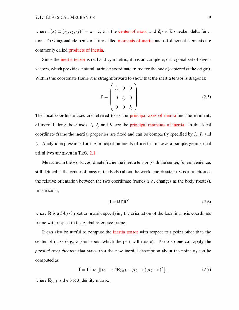


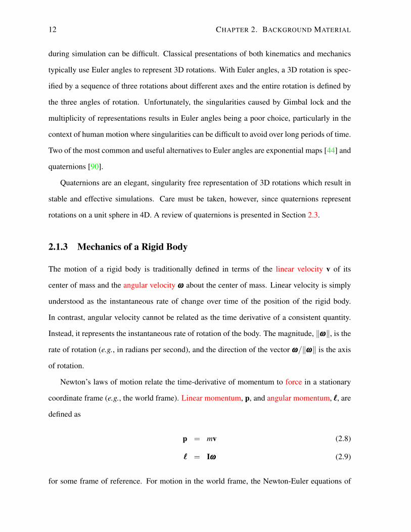
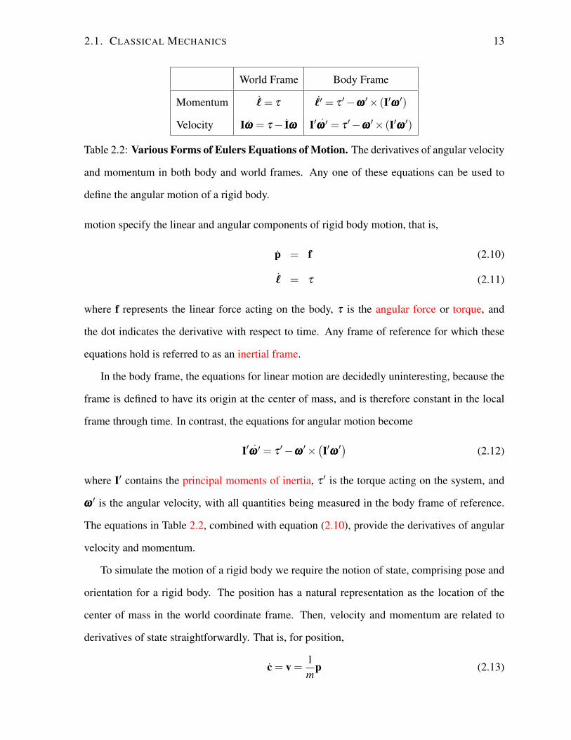
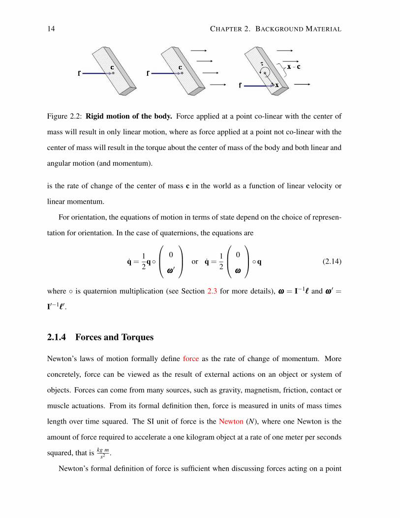
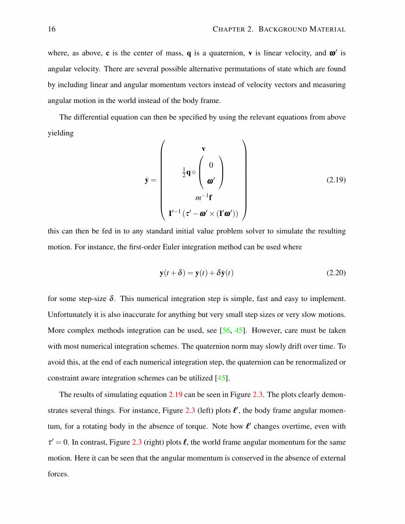
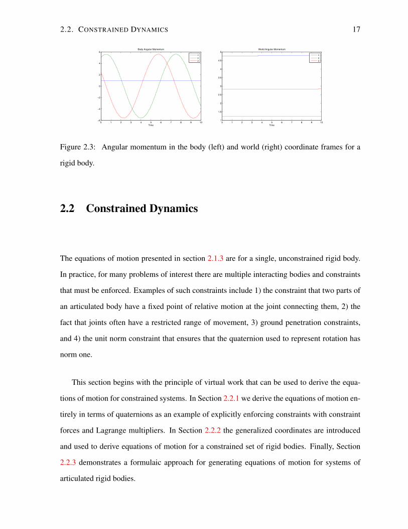


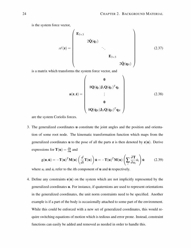
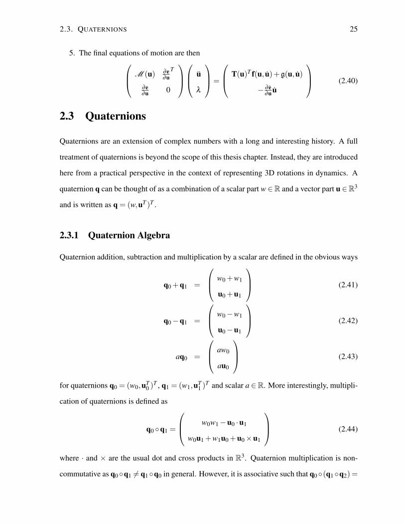


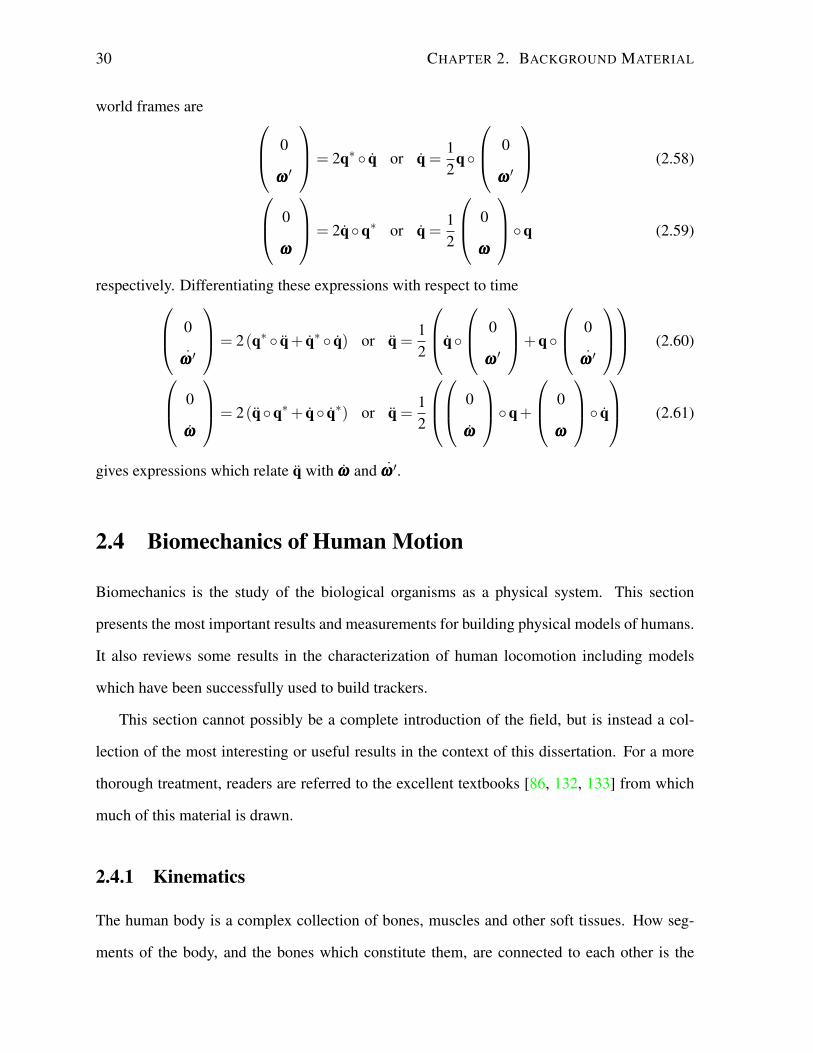
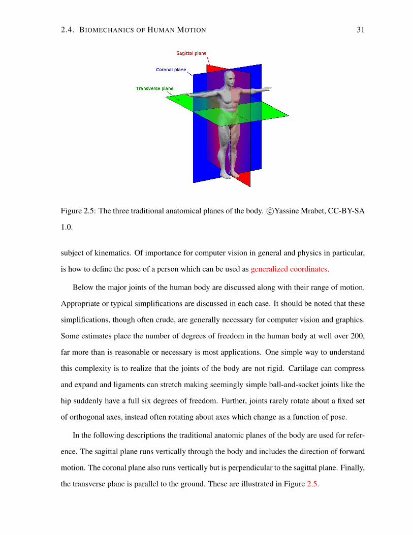


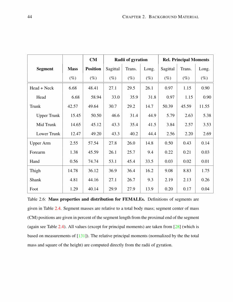


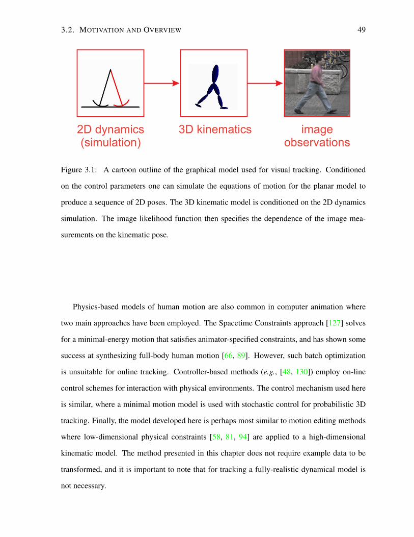


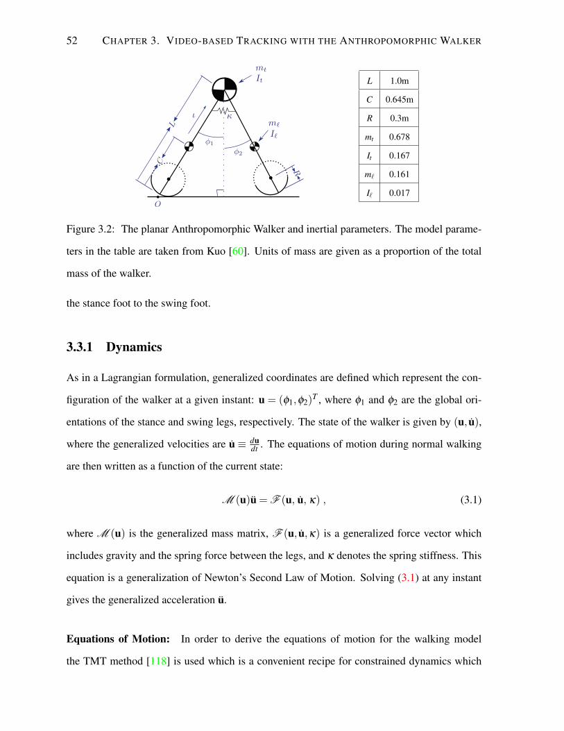


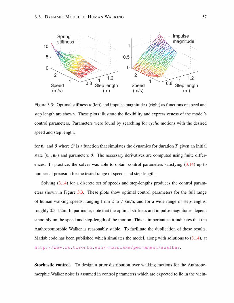
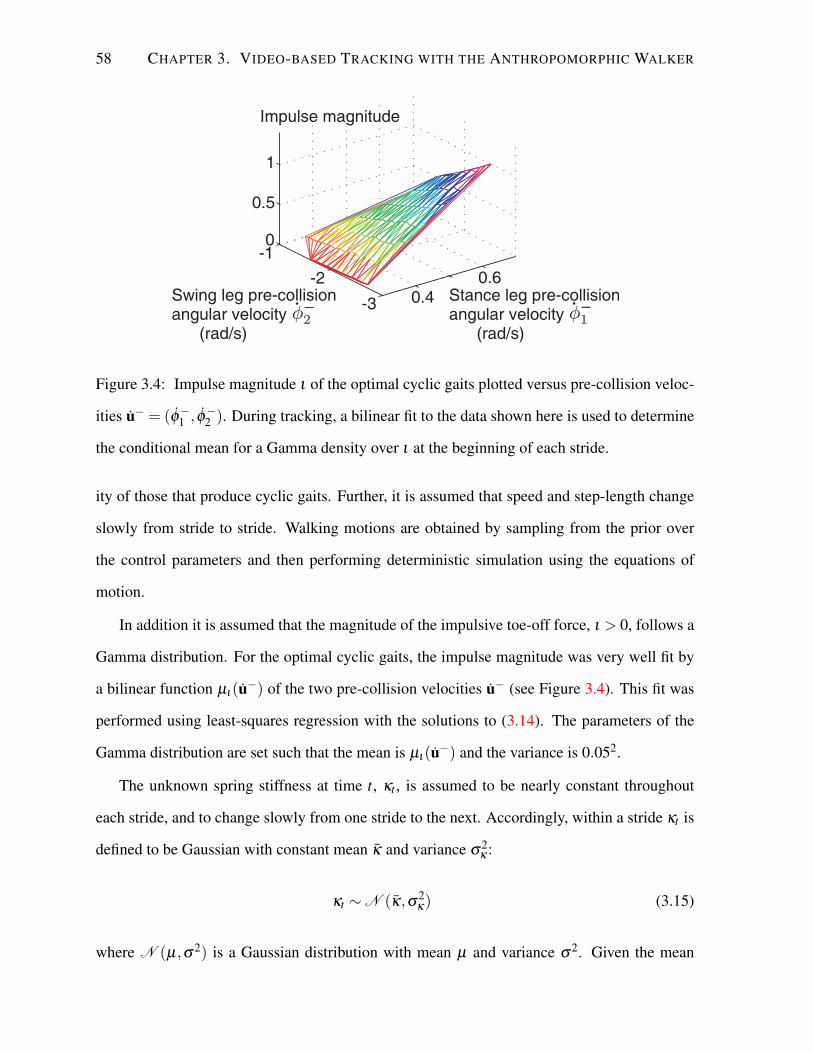
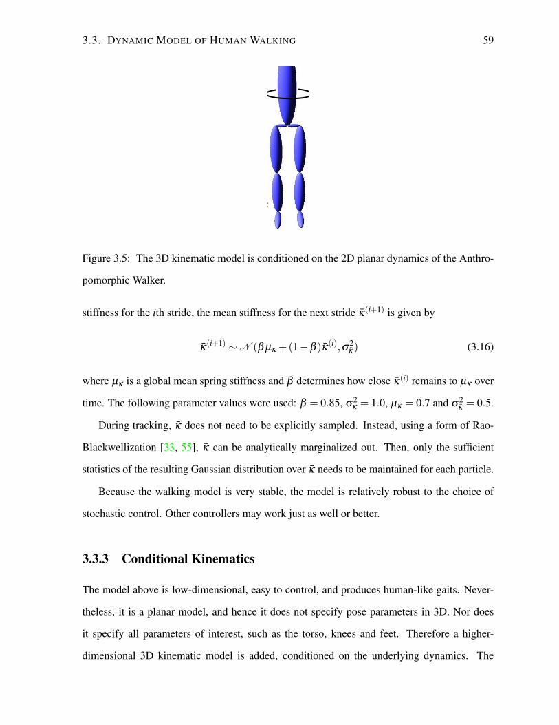

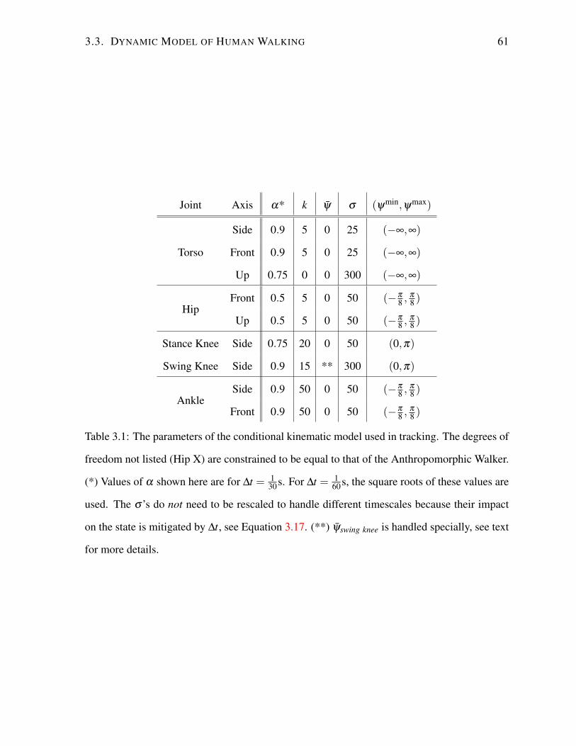
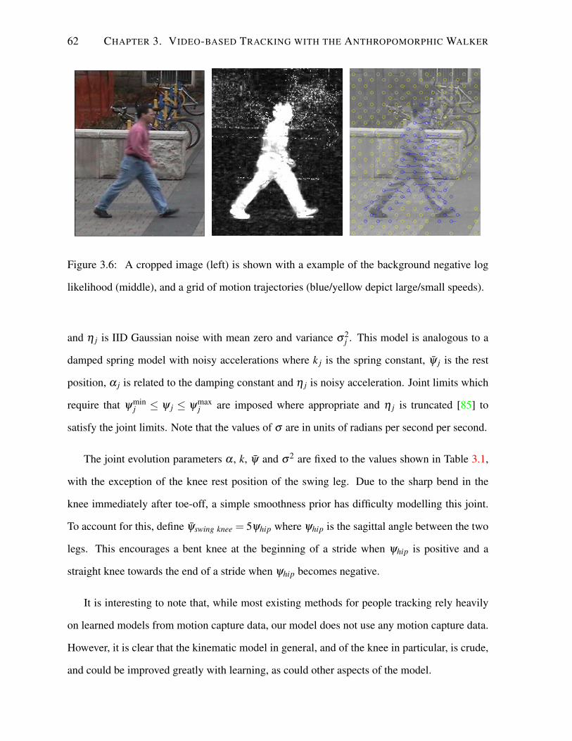
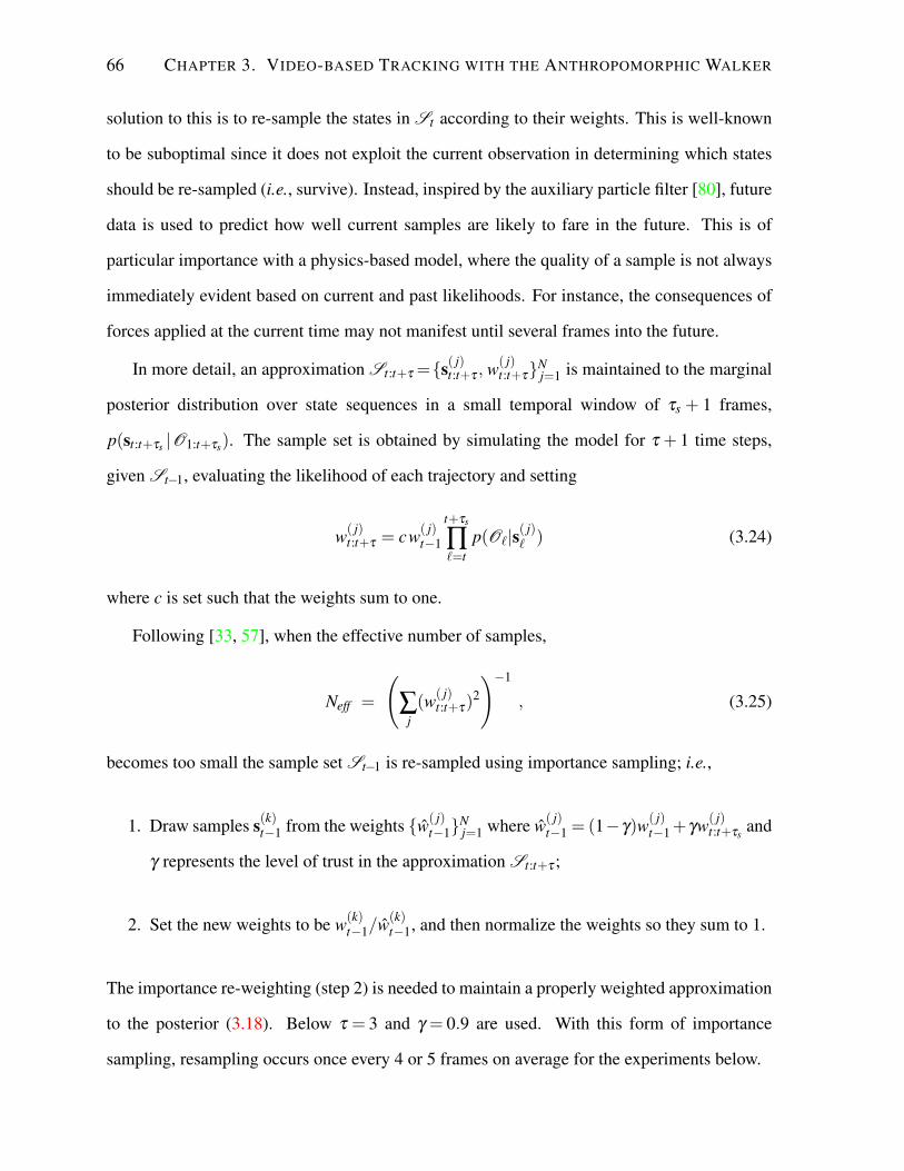
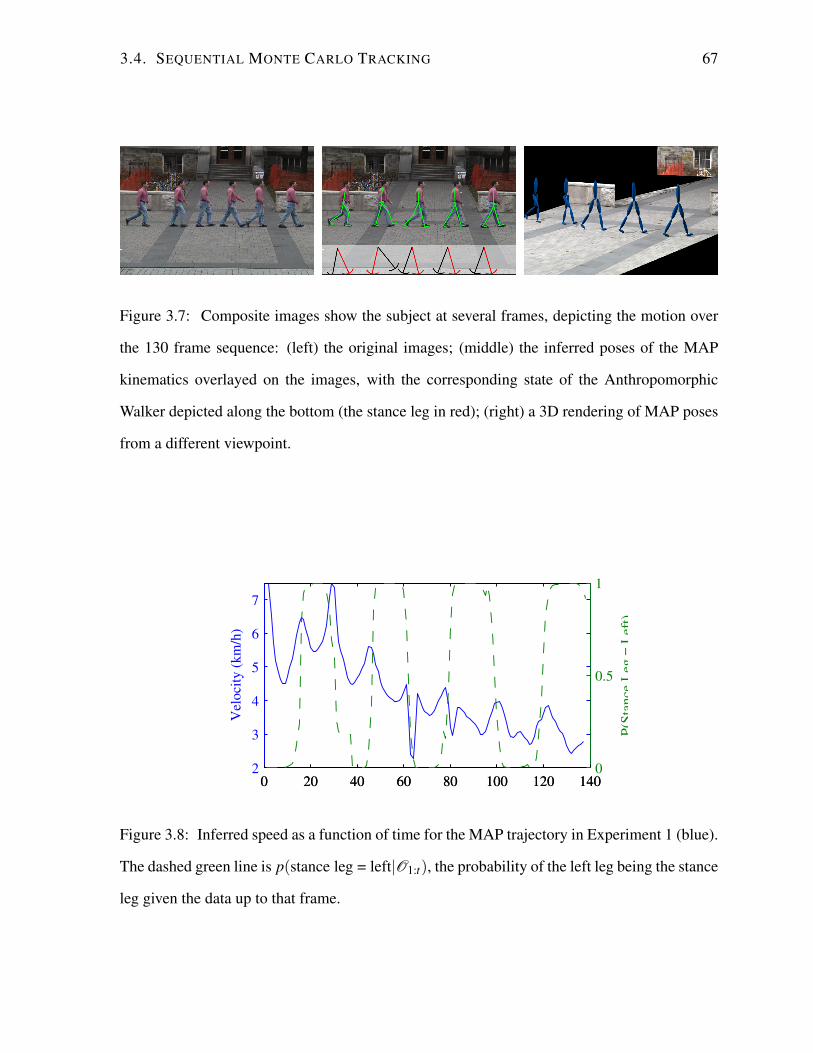
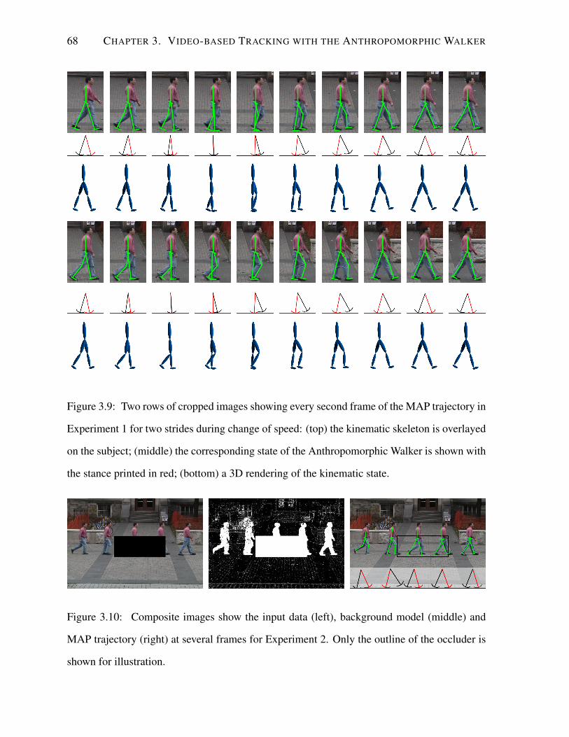
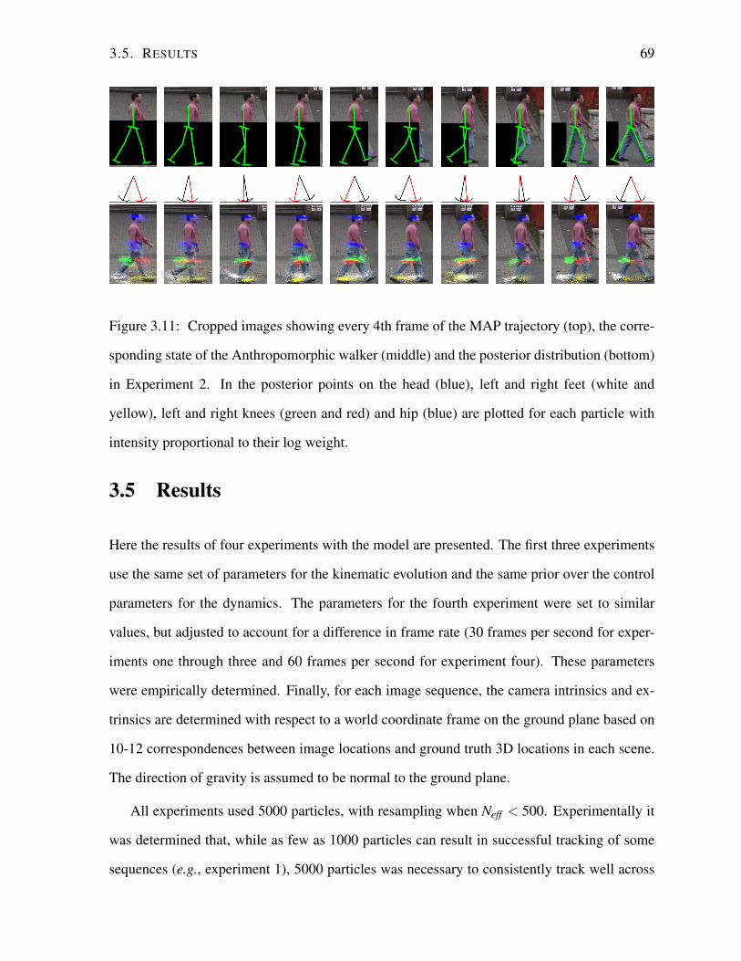
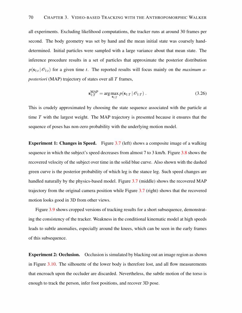
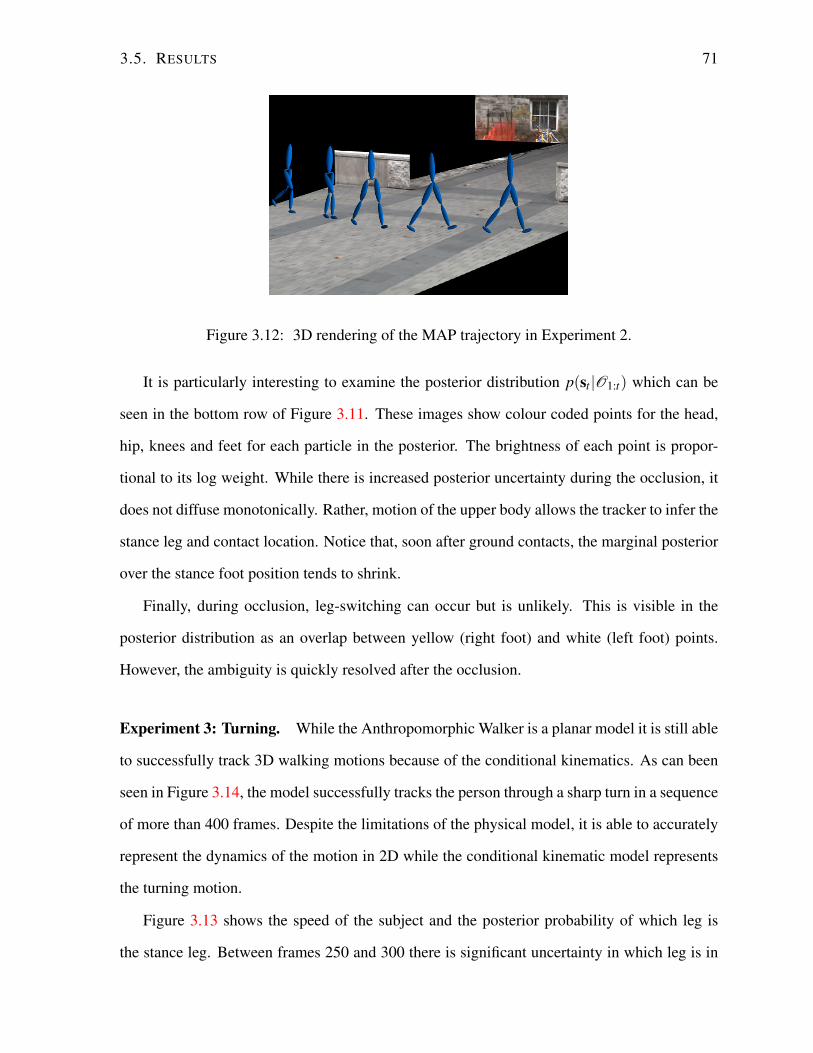
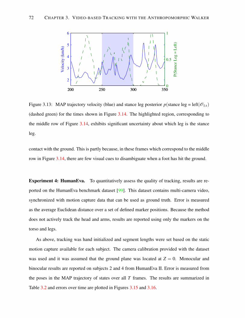


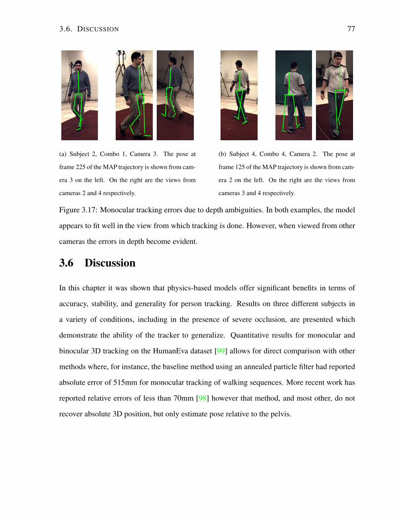


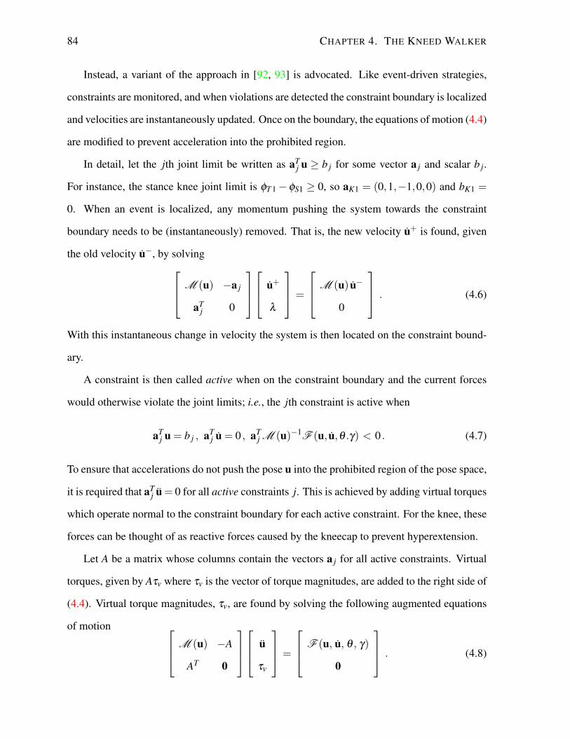
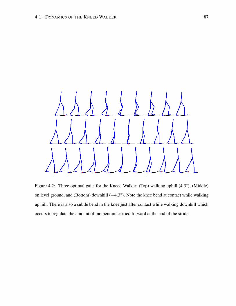

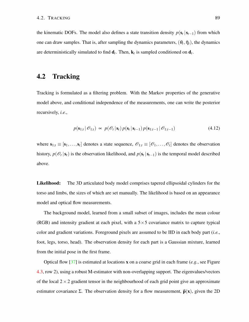
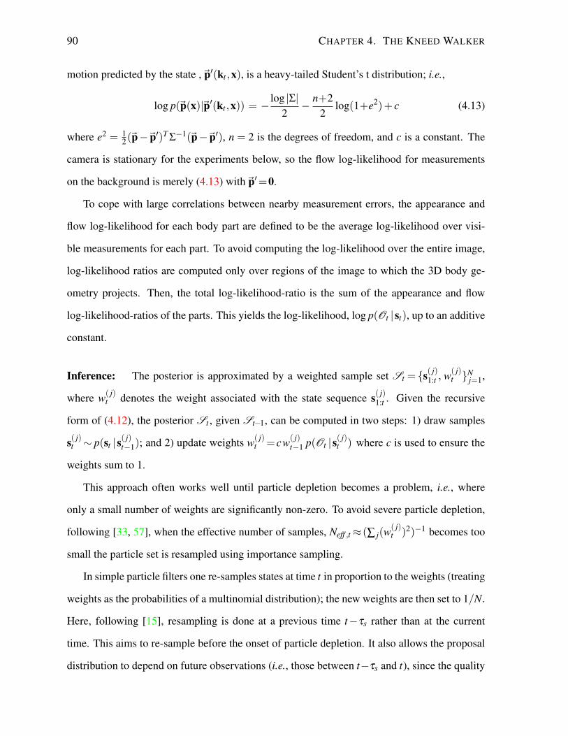

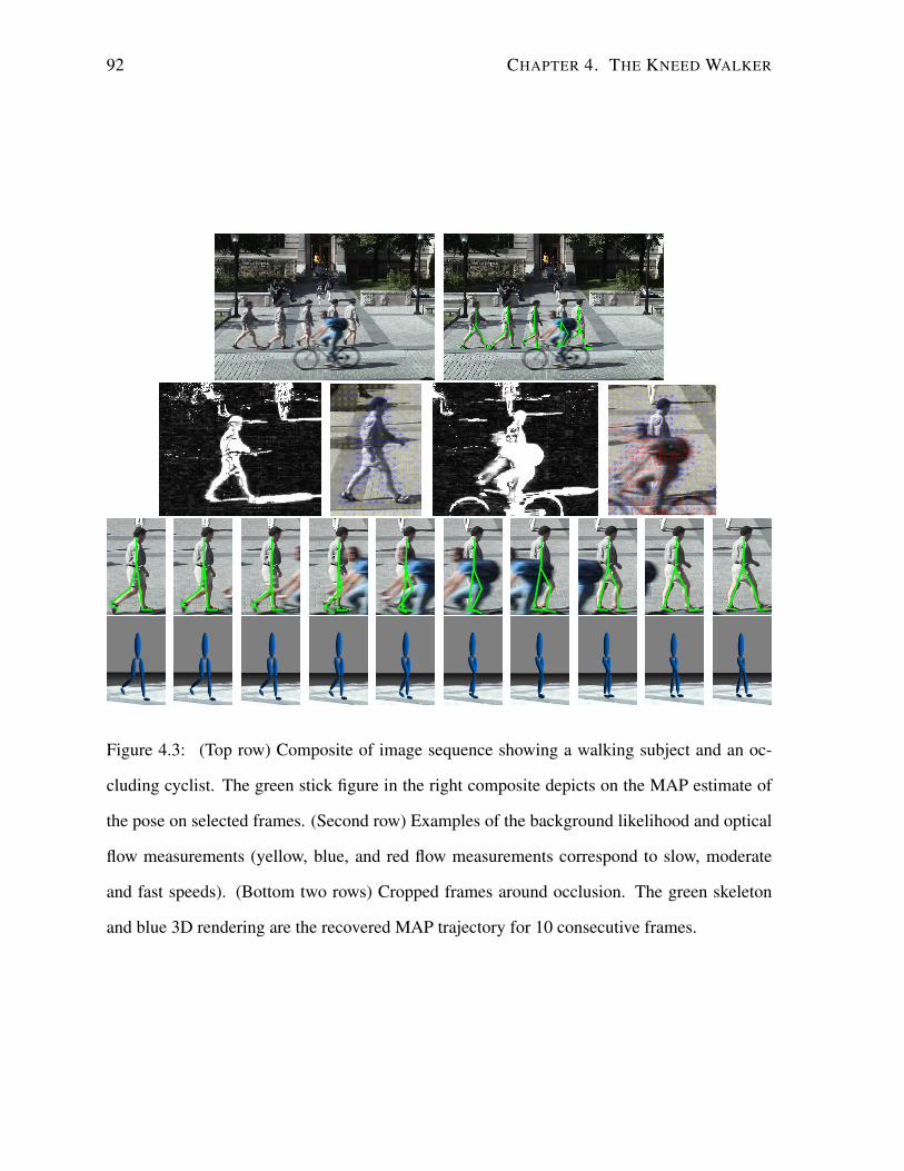
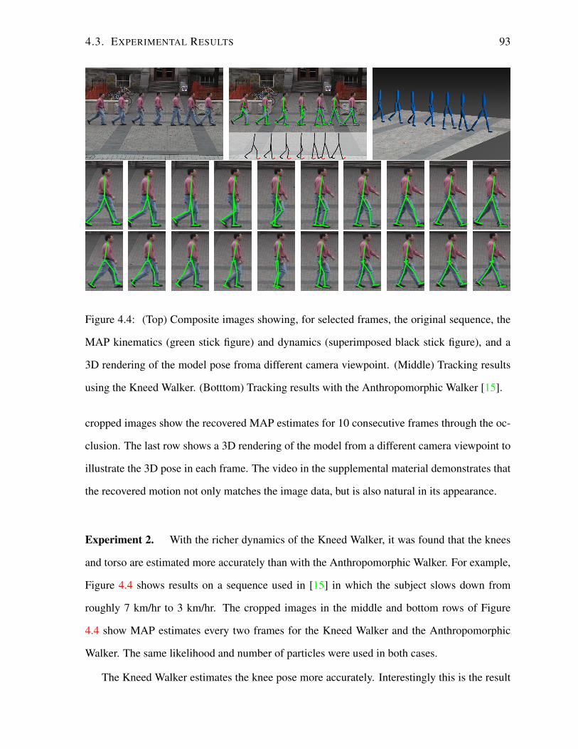
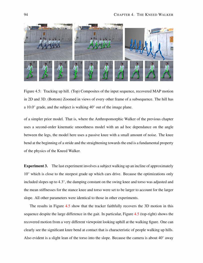
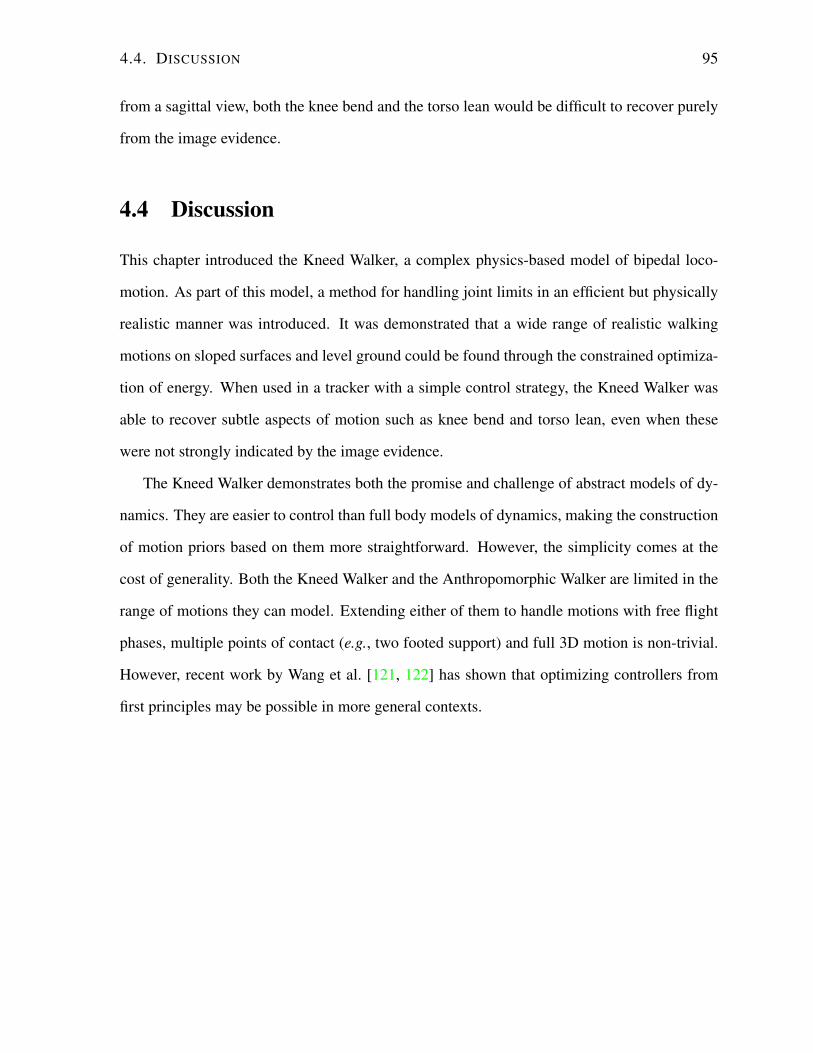

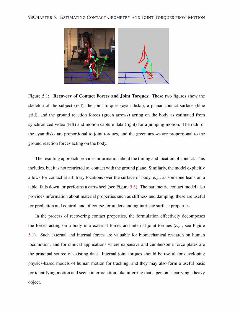


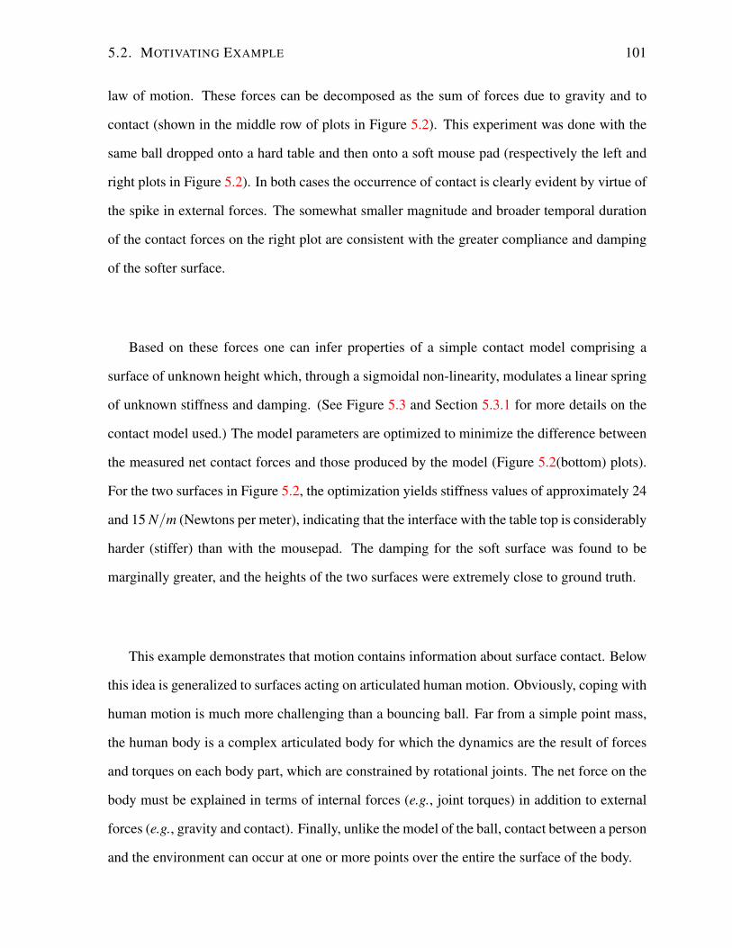

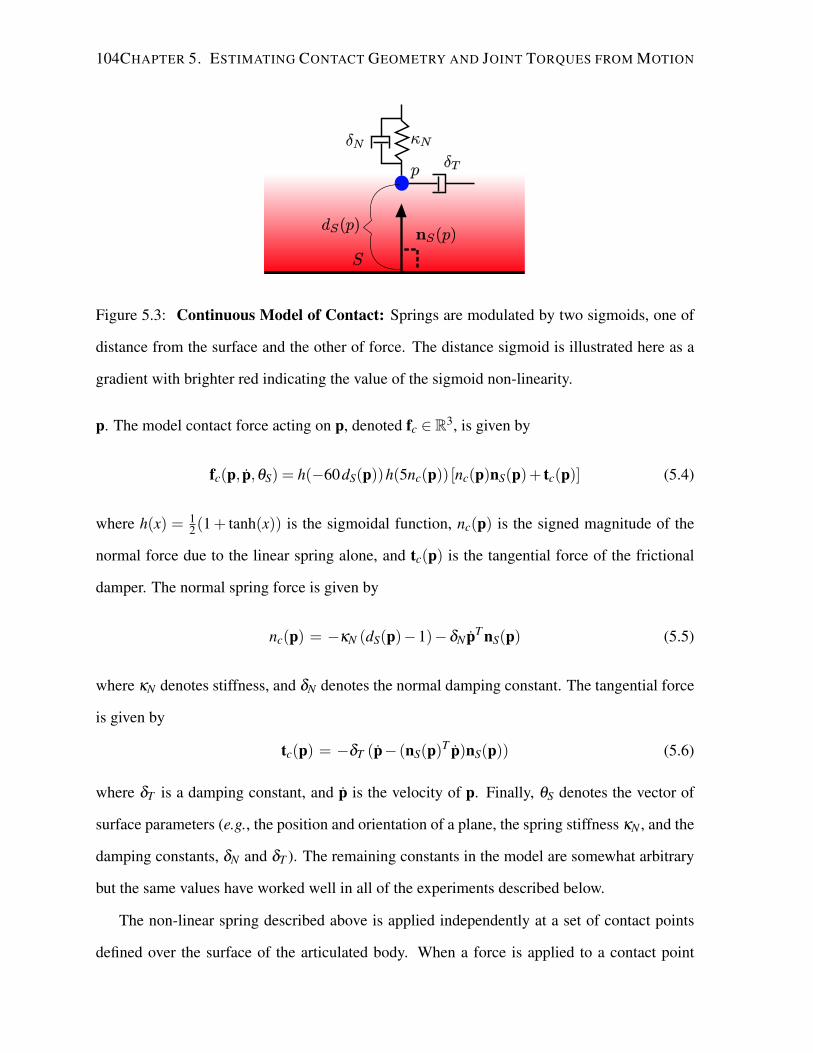
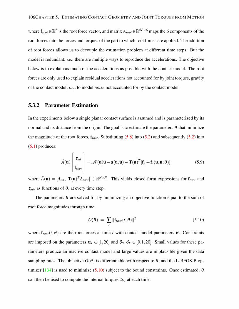

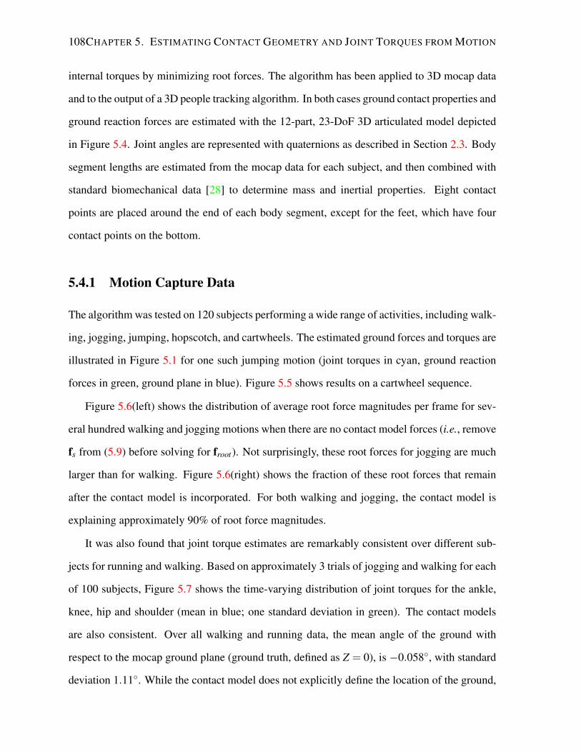
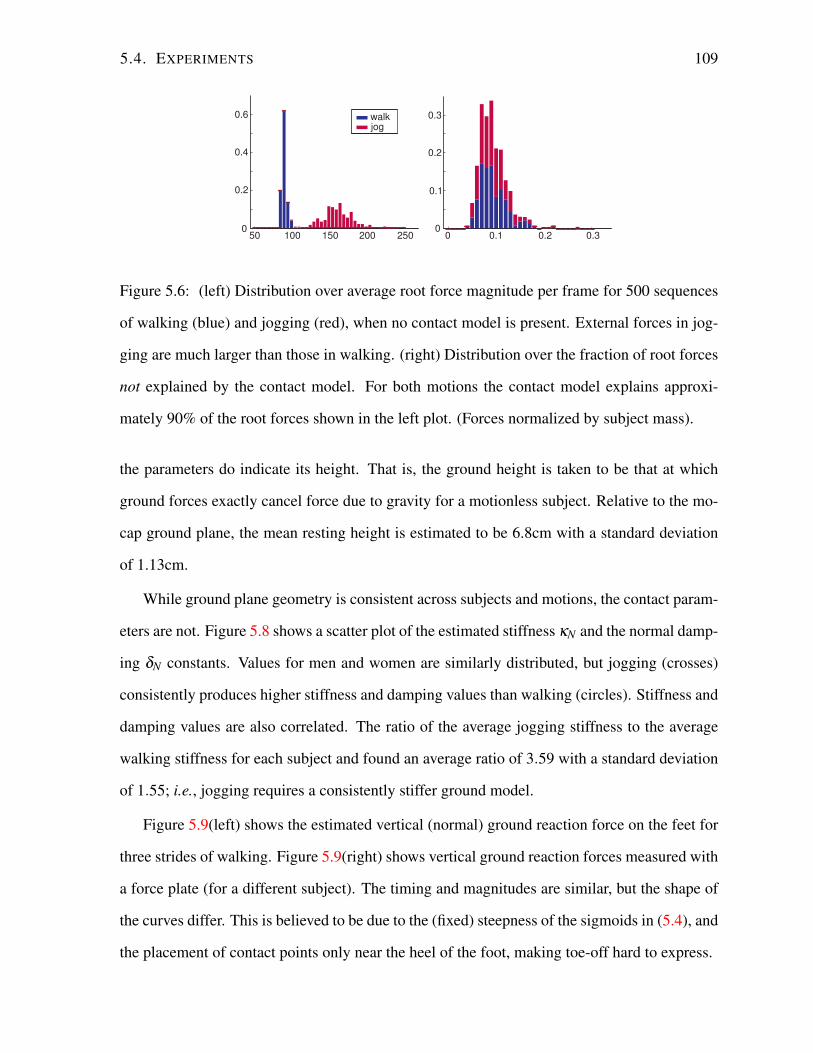
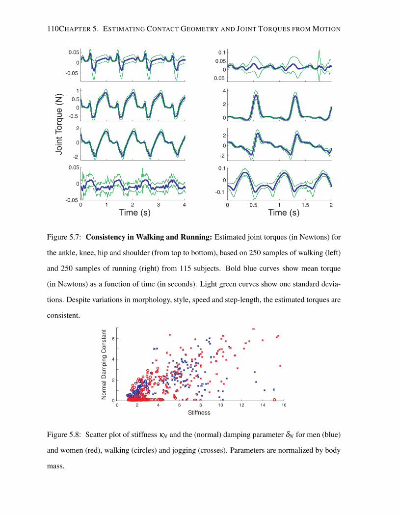

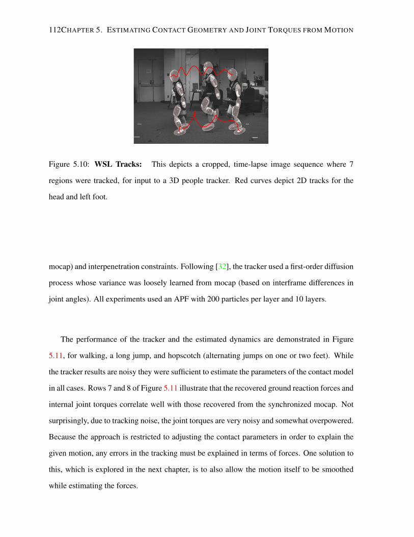
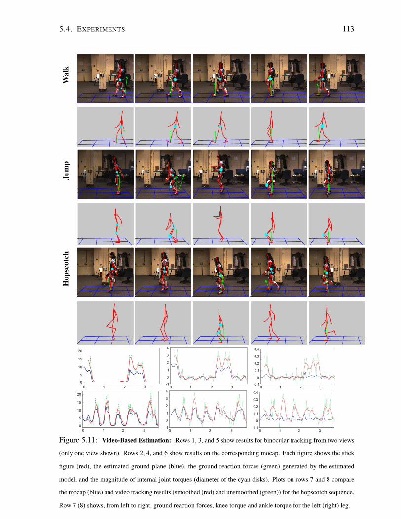


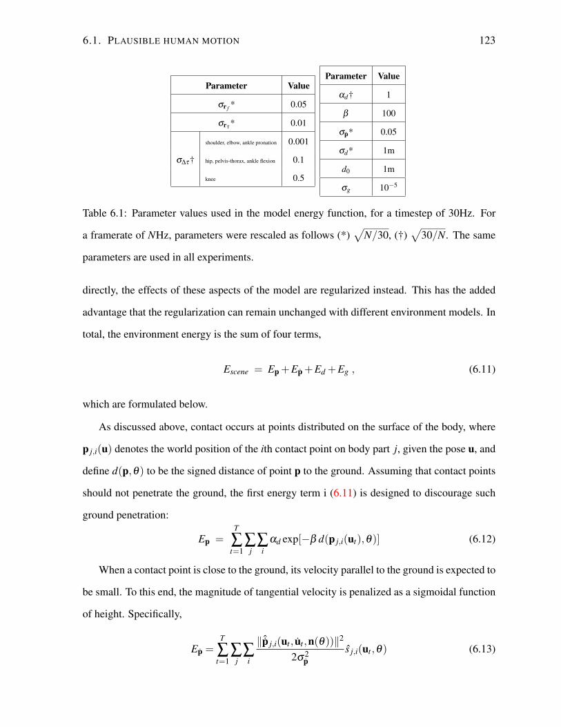
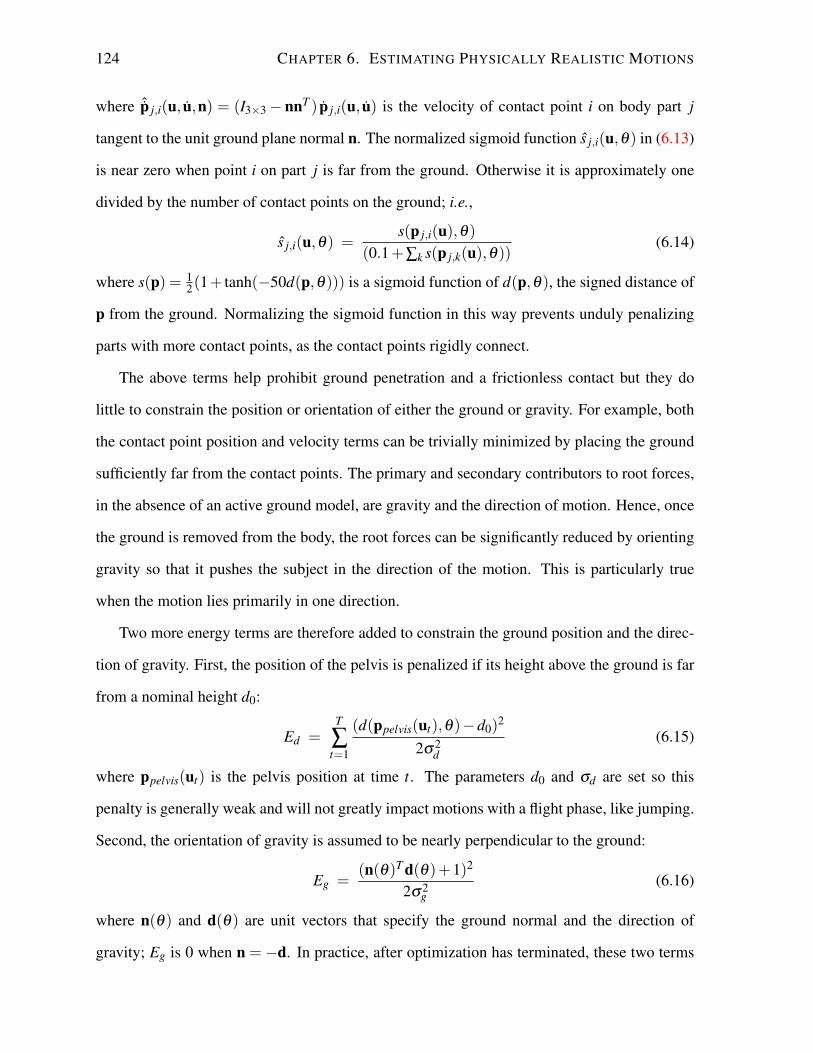


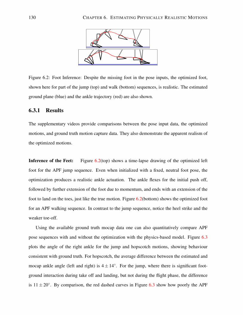
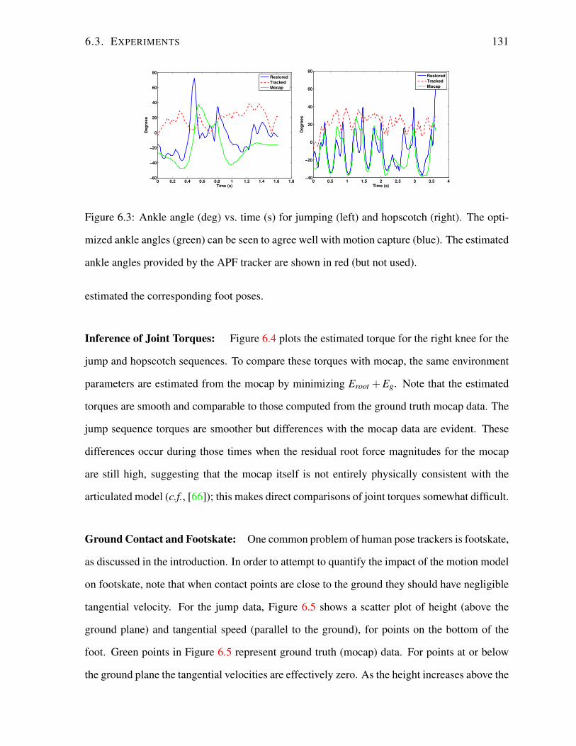

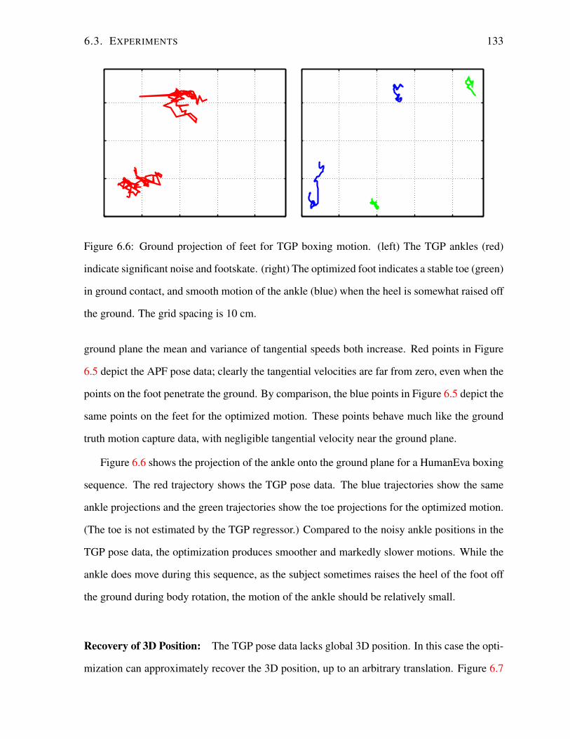


![[Rogers Brubaker] Ethnicity Without Groups](https://static.documents.pub/doc/80x56/5460995eaf79593f708b5515/rogers-brubaker-ethnicity-without-groups.jpg)


