Page 1
MODELING AND ASSESSMENT OF ENERGY MANAGEMENT CHALLENGES
FOR DISTRIBUTED WIND FARMS
By
RAMYAA PARTHASARATHY
A thesis submitted to the
School of Graduate Studies
Rutgers, The State University of New Jersey
In partial fulfillment of the requirements
For the degree of
Master of Science
Graduate Program in Electrical and Computer Engineering
Written under the direction of
Prof. Hana Godrich
And approved by
_____________________________________
_____________________________________
_____________________________________
New Brunswick, New Jersey
October, 2017
Page 2
ii
ABSTRACT OF THE THESIS
MODELING AND ASSESSMENT OF ENERGY MANAGEMENT
CHALLENGES FOR DISTRIBUTED WIND FARMS
By RAMYAA PARTHASARATHY
Thesis Director:
Dr. Hana Godrich
The advent of deregulation of electricity to meet the increasing load demands and
the call for more efficient sustainable energy practices, have dominantly amplified the
need for incorporation of renewable energy systems in today’s power networks. Wind
energy systems can be a leading source of renewable energy with adequate exploration
into the uncertainty surrounding its dependency on climatic changes.
The aim of the thesis is to analyze the potential of energy savings through the
inclusion of wind energy in the already existing network. Wind, in conjunction with the
conventional power generators, needs to meet the continuously varying load demand
while considering the technical real-time constraints imposed by the system. The output
from conventional generators is deterministic while in the case of wind, due to its
Page 3
iii
stochastic nature, the output is intermittent. This is modeled by Weibull probability
distribution function due to its discontinuous behavior.
The first step involved in planning and operating the power system with a wind
farm, is providing a load flow solution. Among various techniques, Newton-Raphson is
one of the most widely used methods to calculate the total generation and line losses
involved in transmission. The next step is to use the load flow solution to optimize the
economic dispatch of the real power in the system. The optimal allocation of the
generated power among conventional and wind units are based on the operating cost of
the units and the cost of wind power. The cost of wind units accounts for various
scenarios such as the penalty cost due to overestimation and underestimation of wind
power and the direct cost pertaining to the issue of ownership of the wind generators.
The research involved in this thesis provides a novel model for power system
operation combining conventional and renewable energy along with remote energy
storage systems, which are validated effectively for the proposed system. Furthermore,
with the help of the Newton-Raphson load flow technique followed by economic
dispatch, an efficient and economical solution is provided to determine the optimal output
at the lowest cost while keeping the transmission and other operational constraints in
check.
Page 4
iv
Acknowledgement
First and foremost, I would like to express my sincerest and deepest gratitude to
my advisor, Professor Hana Godrich, who has supported and guided me throughout my
thesis with utmost patience. Her keen perspective, acute engineering insights, wide
knowledge and constructive comments has been of been great value for my thesis.
I would also like to thank the members of my defense committee, Professor Zoran
Gajic, and Professor Michael Caggiano for being a part of my thesis committee and for
providing invaluable insights and comments.
I would also like to thank all my colleagues, namely Mr. Joseph Amato, Mr.
Christopher Kim Reyes, and Mr. Barney Leinberger who constantly helped me with my
dissertation and proof-read my work. Their keen, sharp eyes, and grammatical advice on
my thesis proved very valuable and greatly enriched my work.
Finally, I would also like to thank the Electrical and Computer Engineering
Department faculty, the staff, and my fellow classmates. I appreciate their unfailing
support and confidence in me.
Page 5
v
Contents ABSTRACT OF THE THESIS................................................................................................ ii
Acknowledgement ...................................................................................................................... iv
List of Illustrations ................................................................................................................... viii
List of Tables ................................................................................................................................ x
CHAPTER 1: Introduction ........................................................................................................ 1
1.1. The Need for Electricity and the Growing Importance of Renewable Energy .... 1
1.2. Urbanization and Mega-cities .............................................................................. 3
1.2.1. Energy consumption ..................................................................................... 5
1.2.2. Population explosion ..................................................................................... 6
1.2.3. Megacity trends ............................................................................................. 7
1.3. Eco-city ................................................................................................................ 8
1.4. Smart Grid ............................................................................................................ 9
1.4.1. Smart Grid – Motivation and Objectives .................................................... 10
1.5. Impact on Economy ........................................................................................... 11
CHAPTER 2: Wind Energy .................................................................................................... 13
2.1. Historical Background and Development of Wind Turbines ............................. 13
2.2. Current Status of Wind Energy .......................................................................... 14
2.3. Wind Resources.................................................................................................. 21
2.4. Advantages and Disadvantages .......................................................................... 22
2.5. Wind Energy and Quality / Extracting Energy from the Wind .......................... 23
2.6. Wind Turbine Efficiency .................................................................................... 25
2.7. Factors Affecting Wind Energy: ........................................................................ 26
2.7.1. Velocity of the wind.................................................................................... 26
2.7.2. Air Density .................................................................................................. 27
2.7.3. Betz Ratio.................................................................................................... 27
2.8 Wind Machinery and Generating Systems ......................................................... 28
2.8.1 Vertical - Axis Wind Turbine ..................................................................... 29
2.8.2 Horizontal- Axis Wind Turbine .................................................................. 30
2.9 Major Components of the Turbine ..................................................................... 31
Page 6
vi
2.9.1. Rotor ........................................................................................................... 33
2.9.2. Nacelle: ....................................................................................................... 33
2.9.3. Tower .......................................................................................................... 34
2.9.4. Blades .......................................................................................................... 34
2.9.5. Controller .................................................................................................... 34
2.9.6. Transformer: ............................................................................................... 34
2.10 Integration into the Wind ................................................................................... 35
2.11 Economics of Wind Power ................................................................................. 36
CHAPTER 3: Newton Raphson Load flow and Economic Dispatch ............................... 38
3.1 Power Flow Analysis ......................................................................................... 38
3.2 Classification of Buses ....................................................................................... 38
3.2.1 Slack Bus or Swing Bus or Reference Bus ................................................. 39
3.2.2 Generator Buses or Voltage Controlled Buses ........................................... 40
3.2.3 Load Buses .................................................................................................. 40
3.3 Load Flow/ Power Flow Techniques ................................................................. 41
3.3.1 Load Flow Objectives ................................................................................. 41
3.4 Newton Raphson Load Flow Analysis ............................................................... 42
3.4.1 The Formulation of Admittance Matrix, Real and Reactive Power ........... 42
3.4.2 Data for the Power Flow ............................................................................. 45
3.4.3 Power Flow Method .................................................................................... 46
3.5 Modified Newton Raphson Power Flow ............................................................ 49
3.5.1 Wake Effect ................................................................................................ 49
3.5.2 RX Bus Model with Wind Farm ................................................................. 51
3.5.3 Algorithm .................................................................................................... 57
3.5.4. Flow Chart: ................................................................................................. 58
3.6 Economic Dispatch ............................................................................................ 59
3.6.1. Objective of Economic Dispatch Problem .................................................. 60
3.6.2. Constraints of the Economic Dispatch Problem ......................................... 63
3.7 Probability Analysis of Wind Power .................................................................. 66
3.7.1 Wind Speed Characterization ..................................................................... 66
CHAPTER 4: IMPLEMENTATION AND RESULTS ...................................................... 67
Page 7
vii
4.1 Test Case: IEEE 14-Bus Test System ................................................................ 67
4.2 Wind Generator Placement ................................................................................ 68
4.3 Results of the Modified Newton Raphson Power Flow Algorithm ................... 72
4.4 Economic Load Dispatch Model for the Modified Test Case ............................ 83
4.4.1. Effects of Wind Power Coefficients ........................................................... 84
4.4.1.1. Effect of Reserve Cost Coefficient ............................................................. 85
4.4.1.2. Effect of Penalty Cost Coefficient .............................................................. 86
CHAPTER 5: Conclusion and Future Scope ........................................................................ 88
5.1. Conclusion .......................................................................................................... 88
5.2. Future Scope ....................................................................................................... 90
5.2.1. Algorithm Optimization .............................................................................. 90
5.2.2. Incorporation into Smart Grids ................................................................... 91
5.2.3. Storage System............................................................................................ 91
Bibliography ............................................................................................................................... 92
Page 8
viii
List of Illustrations
Figure 1 Movement of GDP with change in Energy Consumption in the World ............... 2
Figure 2 US Electricity Consumption and Per Capita GDP Growth .................................. 2
Figure 3 Electricity Sales by Sector .................................................................................... 3
Figure 4 Distribution of Energy Across the World ............................................................. 4
Figure 5 Energy Consumption Across the World ............................................................... 5
Figure 6 Energy Consumption Per Capita .......................................................................... 5
Figure 7 World PopulationGrowth ..................................................................................... 6
Figure 8 Global Cumulative Installed Wind Power Capacity- 2006 to 2016 ................... 15
Figure 9 Cumulative Wind Power and Installation Capacity Around the World ............. 16
Figure 10 Cumulative Capacity of Wind Energy across the World ................................. 17
Figure 11 Consumption and Generation of WInd Energy across North America ............ 18
Figure 12 Wind Power Capacity in North America.......................................................... 19
Figure 13 Conversion from Wind Energy to Electrical Energy ....................................... 25
Figure 14 Steady State Wind Speed - Power Curve ......................................................... 26
Figure 15 Wind Energy Conversion System .................................................................... 28
Figure 16 Wind Turbine Configurations........................................................................... 29
Figure 17 Horizontal-Axis Turbine Parts ......................................................................... 32
Figure 18 Turbine Components ........................................................................................ 33
Figure 19 Components of a WInd Turbine ....................................................................... 34
Figure 20 Classification of Buses ..................................................................................... 39
Figure 21 Wake Effect ...................................................................................................... 50
Page 9
ix
Figure 22 Generator's Equivalent Circuit Discounting Stator Impedance ........................ 51
Figure 23 Flow Chart for NR Power Flow with Wind ..................................................... 58
Figure 24 Wind Energy Availability over a Day .............................................................. 61
Figure 25 IEEE 14 Bus Single Line Diagram ................................................................... 67
Figure 26 Modified IEEE 14 bus with Wind Turbine [PSAT Model] ............................. 69
Figure 27 Power Flow Model for Iteration1 ..................................................................... 76
Figure 28 Power Flow Model for Iteration2 ..................................................................... 79
Figure 29 Power Flow Model for Iteration 3 .................................................................... 82
Figure 30 Effect of Reserve Cost Coefficient on the Output ............................................ 85
Figure 31 Effect of Penalty Cost Coefficient .................................................................... 86
Page 10
x
List of Tables
Table 1 Bus Variable Values ............................................................................................ 40
Table 2 Wind Turbine Parameter ...................................................................................... 68
Table 3 Line Data for Modified IEEE 14 Bus with Wind Farm ....................................... 70
Table 4 Bus Data for Modified IEEE 14 Bus with Wind Farm ........................................ 71
Table 5 Convergence characteristics and power system values ....................................... 72
Table 6 Load Flow for Iteration1 ...................................................................................... 74
Table 7 Line Flow and Losses for Iteration1 .................................................................... 75
Table 8 Load Flow for Iteration 2 ..................................................................................... 77
Table 9 Line Flow and Losses for Iteration 2 ................................................................... 78
Table 10 Load Flow for Iteration 3 ................................................................................... 80
Table 11 Line Flow and Losses for Iteration3 .................................................................. 81
Table 12 Generator Data for Modified IEEE 14 Bus Test System ................................... 83
Table 13 Parameters of Wind Power Plant ....................................................................... 83
Page 11
1
CHAPTER 1:
Introduction
1.1. The Need for Electricity and the Growing
Importance of Renewable Energy
One of the most important factor for development of social and economic growth
today's modern world is the availability of electricity [3] While Graph 1 depicts the
relationship between energy consumption and prosperity for various countries around the
world, Graph 2 depicts the relation between the 2 factors from 1960 to 2010 in the US.
[4] Thus it is clear that over the past 50 years, the Gross Domestic Product (GDP) per
capita has increased with an increase in the electricity consumption per capita. Should
we continue this upward trend, it can be expected that this consumption will only
continue to increase. The main cause behind this assumption is the constant pressure on
power generation utilities to meet the demands of a growing world population and growth
in industrial development to meet their electrical demands.
Page 12
2
Figure 1 Movement of GDP with change in Energy Consumption in the World
Figure 2 US Electricity Consumption and Per Capita GDP Growth
Page 13
3
The above graph provides us with important data from the EIA which represents
the consumption of electricity. Although the numbers constantly keep varying and follow
a stochastic pattern, nevertheless they provide an annually estimated arrangement. Thus,
we notice that the annual consumption of energy resources in the United States has been
at an all-time high and is projected to increase through 2040, in all the three sectors
(commercial, residential and industrial). In 2015, US consumed almost 3.7 trillion
kilowatt-hours (kWh) of energy and it's projected that the total sales would rise 0.7%
annually through 2040. [5]
Figure 3 Electricity Sales by Sector
1.2. Urbanization and Mega-cities
Over the past decades, cities around the world have experienced enormously
unprecedented economic development. This in turn has contributed to a population
Page 14
4
increase through rapid and uncontrolled growth. The result has been the enhanced
environmental pollution and increase consumption of energy resources.
These issues were described by Thomas L. Friedman in "Hot, Flat and Crowded",
2008. He discussed the improper use of energy leading to Global warming due to the
increase of greenhouse gasses. As shown in Graph 4, the unequal distribution of
available energy is a major contributing factor. While countries such as United States,
Canada and other industrialized nations have high energy resources available at their
disposal, developing nations such as Bangladesh and countries in Africa depend on
developing countries for energy.
Figure 4 Distribution of Energy Across the World
Page 15
5
1.2.1. Energy consumption
Comprehending the flow of materials and the drivers of energy in cities is vital for
addressing the environmental challenges at a global scale. Accessing, sharing, and
managing energy and material resources is particularly critical for megacities, which face
enormous social stresses because of their sheer size and complexity.
Figure 5 Energy Consumption Across the World
Figure 6 Energy Consumption Per Capita
Page 16
6
1.2.2. Population explosion
In the 19th century the world population crossed the 1 billion mark. Post this, the
rate of increase in population was exponential. Currently the world population stands at 7
billion. Before the 19th century the deaths were caused by critical reasons like epidemic,
famine or both together. With the advancement in science and technology the health
conditions improved, elimination of deadly diseases like small pox, better transportation,
well connected canals for irrigation. These advancements have led to decrease in
mortality rate.
As the population is rising, so is the energy demand increasing. The per capita
energy needs have also increased with improvement in living conditions, increase in
standard of living etc. The growth in world population has also put a tremendous strain
on the energy industry so that they can meet these demand supply gap.
Figure 7 World Population Growth
Page 17
7
1.2.3. Megacity trends
According to the OECD and the World Economic Forum, the contribution from
the energy industries to the GDP of the United States has grown from 4% in 2009 to
5.9% in 2016. [6]Out of this, the EIA estimated that 65% was generated from fossil fuels,
about 20% of nuclear energy and only 15% from the renewable resource. [7]This rising
demand is a potential cause for the deterioration of the environment because of the
combustion of fossil fuels to meet the energy requirements. So, in order to keep meeting
the generation capacity while ensuring minimum carbon dioxide emissions, more
emphasis needs to be put on renewable energy resources. Among the various renewable
energy resources, wind energy has been considered by far the most promising resource.
[8]
Page 18
8
In the past two decades, wind energy has proven to be one of the fastest growing
technologies. Moreover, with the increasing technological advancements, harvesting
wind energy has proven to be highly reliable, profitable and efficient. As per the
American Wind Energy Association (AWEA) press release, US lead the world in wind
energy production, which has tremendously increased from 4.7% in 2015 to 5.6% in 2016
and is forecasted to increase to 20% by 2030. [9]
1.3. Eco-city
Socio and economic modernization throughout the world have brought about booms
as nations attempt to strengthen their economic growth. These societal changes are
accompanied by two major issues that nations need to address, a population growth
explosion and a shortage of energy for the masses. As counties reach this point in their
growth, a balance needs to be reached between nature, energy, food, water and
necessities, and the economic growth of the nation. [1] The aim is to building self-
sustaining cities and neighborhoods, one would be able to reduce the ecological footprint
and make for a more environment friendly place. This point is coined with the term Eco-
City or Sustainable City, a term coined by urban theorist and author Richard Register.
He theorizes that by creating this type of environment nations would reduce water and air
pollution, caused by methane, CO2, etc., while supplying its own energy, food, water and
necessities.
In creating a sustainable city, the interaction between technology and human
behavior is vital. Large stakeholders need to be involved in creating and running of such
an infrastructure. A current example of this type of Eco-City is Sino-Singapore Tianjin
Page 19
9
Eco City in China. It is considered a landmark project, using smart grid construction that
uses wind and photovoltaic power, integrated into the micro grid. The Eco-City grid
helped in reducing the fuel consumption by 1,074 tons per year and saved 5,930 tons of
coal. Other new technologies such as auto-distribution, equipment on-line monitoring,
intelligent scheduling and substations were adopted that improved power quality and
power supply reliability. [2]
These types of ideas combined with the promotion of renewable energy are here
today. Combining these technologies, along with a sustainable energy philosophy, and
an increase of technological innovations that target building a viable, affordable and
highly reliable renewable source are the future and will help us in creating a smart and
efficient energy infrastructure.
1.4. Smart Grid
With the increasing demand for power and electricity, more power plants and
transmission and distribution facilities are built to meet the needs. However, these
modifications are very expensive and are hard to achieve while keeping the
environmental regulations in check. So, alternatively, it’s imperative to revise the current
power distribution network and harness the renewable energy such as the wind and solar
power in a more efficient way. This approach can be effectively implemented through
smart grid technology as a productive and profitable solution.
A smart grid, although based on the physical grid, is an electrical infrastructure that
integrates renewable energy with advanced computer technology, sensor measurement,
Page 20
10
communication and control technology. [10] The primary target is to manage and
monitor the energy usage by providing a sense of energy independence, which would
provide the liberty to choose when and how to use the electricity. With the help of smart
meters, the users would have a better knowledge about the real time pricing information
of electricity during normal and peak hours which would in-turn optimize the demand
and supply chain use of it.
1.4.1. Smart Grid – Motivation and Objectives
The electrical power grid that still exists today was designed almost fifty years
ago. With the increasing power needs, a lot of pressure is put on these systems, which
results in occasional blackouts causing interruption of services which inadvertently pose
significant safety and economic threats. In such a scenario, smart grids offer a sound
system that allows automatic monitoring and evaluation of the grid conditions. The
various devices on the network have the capability to communicate with each other and
detect and repair faults and automate rerouting if required, at the time of power line
faults. This helps reduce the power outages.
Communication is also possible between the user and the power suppliers through
the help of smart meters. These meters provide a means of accumulating and transmitting
accurate power consumption reports with respect to the quantity of the power used at
specific times of the day, which further provide information such as the real time pricing
and emergency requests to lower consumption when needed.
Newer technologies have been integrated into the smart grid system that is meant
to encourage consumers to invest in distributed generation system, or locally generated
Page 21
11
sources like solar panels on the rooftop of a home, to supplement the needs. [11] For
example, the Pecan Street project near Austin, Texas, integrates a variety of DER
(Distributed Energy Resources) technologies and the residents have not experienced a
power outage in over four years. [12] Moreover, houses could install solar panels and can
power their homes by its solar energy during the day, and sell any extra energy produced
back to the grid.
The smart electric infrastructure presents an unprecedented opportunity to provide an
efficient and reliable structure that will help in our economic and environmental growth.
It is much more than just utilities and technologies, it is about providing the information
and the tools to use energy judiciously.
1.5. Impact on Economy
The increase of dependence on high-quality and reliable energy delivery system has
persuaded out economic security for growth to become more reliant on replenishable
forms of energy. The complete deployment and integration of Smart Grid technologies in
the system will most certainly assuage the pressure put on American businesses as a
result of congestions, power fluctuations, failures of the present electric grid. The vital
step towards improving the American economy at a global level is to increase the energy
efficiency and the reliability of the system.
Several studies suggest that the optimization capacity provided by the smart grid
system will proportionally improve the consistency in energy delivery, reduce waste and
lower the business costs. [13]Although, the impact of power blackouts and power
Page 22
12
inconsistency may affect residential areas on a minor level, at an industrial scale they
could be devastating. One such overwhelming power outage occurred in southern
California in 2003 when the blackout created a loss of approximately $75 billion dollars
and resulted in the collapse of one of the largest energy company in the state, Enron
Corporation [14]. In such a scenario, Smart Grid system will provide the energy security
required to sustain an energy dependent economy by optimizing the system and ensuring
the electrical normalcy is returned within a short frame of time or avoiding the disruption
completely.
Moreover, Smart Grid is helping in the creation of a new market which is gaining
popularity and momentum. This involves developing energy efficient and intelligent
appliances, smart meters and passenger vehicles. Tis would in turn pave a path to new
and enhanced communication procedures and capabilities. According to Department of
Energy, shift to Smart Grid system will create a market for $100 billion in smart
technologies [15]. Consecutively, an additional GDP of $2 trillion dollars will be
created. Therefore, adoption of the Smart Grid has made the market competitive, secure
and given birth to numerous new market opportunities.
Page 23
13
CHAPTER 2:
Wind Energy
2.1. Historical Background and Development of Wind
Turbines
Wind energy is considered to be one of the most abundant renewable resources
and for centuries man has tried to harvest it. It has been predicted that humans have tried
to harness wind energy for about 4000 years in different aspects of their daily work such
as powering sailing ships. The Windwheel of Heron of Alexandria which used the energy
of the passing gusts of wind was one of the first known instances of wind-powered
machinery. [16] As early as the 17th century BC, the emperor of Babylonian, King
Hammurabi used wind-powered scoops for the irrigation of the plains in Mesopotamia.
[17] However, the Panemone windmills were the first practical wind-powered machinery
that was built in Sistan, a region between Afghanistan and Iran, around the 7th century.
[18] They were vertical axle windmills with braided mats utilized to generate drag to rate
the device around a central axis. These windmills were used to pump water and grind
grain and corn. The first wind turbine to generate electricity was built by James Blyth in
Page 24
14
July 1887. He used the electricity to charge accumulators which were then used to power
the lights in his cottage. [19]
So, though wind energy was used for electricity generation in early times, the low
cost of fossil fuels, such as coal and oil, made the harvesting of the wind economically
unappealing. But, with the oil energy crises of 1973 and the growing environmental
concerns about the effect of fossil fuel usage, a new interest was inspired by alternative
energy resources and the research on Wind Electric Systems (WES) or WECS (Wind
Energy Conversion Systems) was invigorating. Thus, over the last few decades, the
WECS technology has given birth to several configurations of wind turbines, which
utilize various types of electric generators.
2.2. Current Status of Wind Energy
The sixth edition of the Global Wind Energy Outlook released on November 14,
stated about 3.7% of the global electricity demand was met by wind power in 2015 and it
was predicted that with the increasing growth of renewable sources the share could reach
up to 12% by the year 2020. The Renewable 2017 Global Status Report states that in
2016, almost 55GW of wind power capacity was added which brought the total global
installed capacity to 487GW. By the end of the year, more than 90 countries had some
kind of commercial power activity.
Page 25
15
Figure 8 Global Cumulative Installed Wind Power Capacity- 2006 to 2016
The above graph depicts a steady growth of installations, happening at a rapid
pace until 2010. From the period of 2009 to 2013, there was an unprecedented decline in
new installations which went as below as 21%. This further affected the industry wherein
the sales and the profit declined incredibly. Although from 2014 onwards, the industry
quickly recovered and then in 2015 the 63.5GW of new capacity was installed which
brought the total to 432.9 GW. In 2016, the new installations went up by 55GW and it’s
predicted to be followed by 68GW in 2017 which is equivalent to an increase of 6.3%.
Page 26
16
Figure 9 Cumulative Wind Power and Installation Capacity Around the World
The data indicates that from the year 2014 to 2018, even though the cumulative
wind power capacity in 2013 illustrated a low growth rate of 12.3%, it increased
tremendously in 2014. [20] [21]
Page 27
17
Figure 10 Cumulative Capacity of Wind Energy across the World
Page 28
18
It is also very interesting to note that 84% of the cumulative capacity (411,172
MW) was contributed by the top 10 countries i.e. China, USA, Germany, Spain, India,
UK, France, Brazil, and Italy. [22]China has been experiencing a boom in wind energy
and currently accounts for 34.7% share of the world’s total installed capacity.
Figure 11 Consumption and Generation of WInd Energy across North America
Page 29
19
Figure 12 Wind Power Capacity in North America
The United States is also gaining momentum and has supplied around 5.55% of
the total electricity generated in the country in 2015. The installed wind power capacity
has doubled from 40,283 MW (2011) to 82,183 MW (2016) over a span of 5 years.
According to the "Electric Power Monthly" Report by U.S. Department of Energy,
Energy Information Administration, the electricity currently produced from wind power
in the USA amounts to about 226.5 terawatt-hours.
A lot of initiatives have been undertaken by the US. Department of Energy
through various lucrative programs. Programs such as the ‘Wind and Water Power
Program’ and the federal production tax credit (PTC) sought to support and accelerate
wind power deployment. Ample opportunities are provided to promote the development
of small scale wind power generation industries. The federal government has issued
Page 30
20
numerous tax- based policies as incentives in order to encourage various companies to
increase production and installations while ensuring that the reliability and efficiency of
the turbines are constantly increasing. These incentives could be structured as tax credits,
renewable electricity standards and grants at the local, state and federal levels. Apart
from this, the Department of Energy also offers short and long-term loans and financial
assistance to help the industries and small scale private wind farm owners to deploy clean
and innovate technologies that reduce the production of harmful gases. According to the
report Wind Vision: A New Era for Wind Power in the United States released by DOE,
the intention is to supply 10% of the country’s electricity from wind power by 2020, 20%
by 2030 and 35% by the year 2050. [23]
Generally, wind turbines capture 20% to 40% of the energy of the wind. So at a
site with average wind speeds of 7 m/s, a typical turbine will produce about 1,100 kWh
per square meter of area per year. If the turbine’s blades are 35 meters long, for a total
swept area of 1,000 square meters, the power output will be about 1.1 million kWh for
the year.
The power output from a wind turbine is a function of the cube of the average
wind speed. In other words, if wind speed doubles, the power output increases eight
times. Also, wind speed increases as the height from the ground increases. For example,
if the average wind speed at 10 meters above ground is 6 meters/second (m/s), it will
typically be about 7.5 m/s (25% greater) at a height of 50 meters. Finally, the power in
the wind varies with temperature and altitude, both of which affect the air density. Chilly
winter winds in Minnesota will carry more power, due to greater air density, than warm
summer winds of the same speed high in the passes of southern California.
Page 31
21
On the other hand, wind turbines operate over a limited range of wind speeds. If
the wind is too slow, they won’t be able to turn, and if too fast, they shut down to avoid
being damaged. Ideally, a wind turbine should be matched to the speed and frequency of
the resource to maximize power production.
Another factor in the cost of wind power is the turbines’ distance from
transmission lines. It is not unusual for remote areas (for example, northern Canada or
Siberia) to have high average wind speeds, but be too far from major electricity demand
centers (cities) for the wind power to be used economically. Considerable wind energy
development has taken place in recent years in U.S. states like Indiana and Illinois, which
are not as windy as North Dakota or Montana but have substantial transmission capacity.
For offshore wind projects, the economics depend on the distance from shore
because turbine foundation costs increase rapidly with increasing water depth. Offshore
wind turbines are generally much larger than land-based turbines. Larger rotors can be
incorporated more easily because large rotor blades can easily be transported by ship.
2.3. Wind Resources
Wind energy is originated by the Sun. The uneven heating caused by the rays of
the Sun heats up the surface of the Earth in an uneven manner which consequently
produces the wind. Only a small fraction of the wind produced near selected locations,
close enough to the surface has sufficient strength to run the wind turbines in order to
generate electricity. Places such as the Great Plains regions in the mid-west, like the
Page 32
22
North and South Dakota, if fully exploited, have the capability to generate 50% of current
US electricity consumption.
2.4. Advantages and Disadvantages
With increasing environmental concerns and exponentially escalating fuel prices,
the research behind the integration of wind power generation with the conventional
power system is also rising. The main target is to reduce the dependency on non-
renewable resources while curtailing the greenhouse gas emissions in order to ensure the
protection of the environment. In addition, after the initial land and capital costs, there is
no other cost involved in the generation of electricity as the cost of the fuel is zero.
However, the intermittent and unpredictable nature of the wind speed which
varies during the day and according to the season makes wind power generation
unreliable and rather difficult to control in terms of frequency and scheduling of
generation. Also, the inability to find a cheap means of storage makes it an undesirable
renewable energy that can be harnessed. Moreover, most of the fields, which have a high
potential such as the Dakotas and other off-shore wind farms are not in a reasonable
proximity to large population areas which in turn require the construction of expensive
high-voltage transmission systems that result in large line losses.
Page 33
23
2.5. Wind Energy and Quality / Extracting Energy
from the Wind
Wind turbine power generation is based on the principle that the kinetic energy of
air can be converted into rotating mechanical power of the turbine blades to generate
electricity. It is therefore essential to know the amount of kinetic energy available and the
amount of extractable energy from the wind.
The power, W, due to the wind velocity relative to the ground is given by the following
equation:
𝑊 =1
2 𝑚𝑉2
Where:
V: wind speed
m: mass flow rate of wind through column of area A
The mass flow rate through an area A is given by:
𝑚 = 𝜌 𝐴 𝑉
Where:
ρ: air density
A: cross-sectional area of column
Page 34
24
On combining the above two equations, we get:
𝑊 =1
2(𝜌 𝐴 𝑉) ∗ 𝑉2
=1
2𝜌 𝐴 𝑉3
This result is highly imperative because we can deduce that the power available in
a cross-sectional area of wind is proportional to the cube of the value of the wind speed.
Thus, if the wind speed is doubled, there will be an eightfold increase in the wind power
relative to the ground.
Mostly, the wind farms experience high wind speeds only for a few hours in a
day. So, with the varying wind velocity, the spectrum-average power plays a crucial role.
𝑃’’(𝑣) = ∫ 𝑃’(𝑣) 𝑓(𝑣)
∞
0
𝑑𝑣
Where:
∫ 𝑓(𝑣) 𝑑(𝑣) = 1∞
0
Where:
f (v): frequency spectrum which is defined as the fraction of the time over a year when
the wind blows at velocity v
Page 35
25
2.6. Wind Turbine Efficiency
According to the first law of thermodynamics, Conservation of mass, the energy
that comes out of the wind turbine over a period of time should equal the energy that fed
into the turbine over the same amount of time. It is not possible to convert all of the
kinetic energy of the wind into mechanical; some of the energy is lost in the atmosphere.
Thus, the output energy is equal to the mechanical energy converted to electricity and the
energy left in the air.
Figure 13 Conversion from Wind Energy to Electrical Energy
The above figure, [24], depicts the similar scenario. The wind enters the turbine at
very high speed. The turbine with a diameter of “D” sweeps a circular area represented
by the blue oval, which is the area available for production of power. The energy is
affected by the velocity of the wind and the density of the air.
Page 36
26
2.7. Factors Affecting Wind Energy:
2.7.1. Velocity of the wind
Figure 14 Steady State Wind Speed - Power Curve
Figure 7, depicts that at very low wind speeds, around 3-4m/s, the cut-in speed,
the power that can be generated is too low to be utilized [25]. The wind turbine is started
at cut-in speed and the power is increased till the moment, the rated speed is reached.
This usually ranges from 12 m/s to 25 m/s. The amount of power produced is limited at
the rated power of the turbine with stall-regulators or pitch-control systems. As soon as
the wind speed exceeds 20-25 m/s, also termed as the cut-out speed, the turbines are
brought to a standstill to avoid the high mechanical loads on the turbine elements.
Page 37
27
2.7.2. Air Density
𝑷’(𝑣) = 𝑃(𝑣)
𝐴= 𝜌 𝑣3
2
So, when the temperature is 1°C and 1 atmosphere, the dry air has a density equal
to 1.226 kg/m3. Now, when the turbine is placed above sea level, for example, in case of
Denver, which is 1.6km above sea level, the air density reduces to 0.84 kg/m3. Moreover,
factors such as water vapor in the air, also decreases the density.
2.7.3. Betz Ratio
The Betz law is analogous to the Carnot cycle efficiency in thermodynamics. It
states that the maximum theoretical power that can be extracted from the wind by a wind
turbine is 16/27 (59.3%) of the total kinetic energy of air flowing through the effective
disk area of the turbine. This ratio, limits the upper bound on the annual energy that can
be extracted at a site. Moreover, as the wind speed varies according to various factors, the
annual capacity of a site is around 25% to 60% of the energy that would be generated
with constant wind.
Page 38
28
2.8 Wind Machinery and Generating Systems
Figure 15 Wind Energy Conversion System
Figure 8, [26] shows how the energy from wind can be harnessed through a Wind
Energy Conversion System (WECS). The system comprises of the wind turbine blades, a
power electronic converter, an electric generator, and a required control system. Although
the functional objective is to convert the kinetic energy into electric power and in turn
inject this power into a utility grid, there are different WECS configurations. These are
based on if they use synchronous or asynchronous machines, and stall-regulated or pitch
regulated systems.
Wind turbines can be further classified according to the orientation of the axis of
rotation with respect to the direction of the wind, which is vertical-axis and horizontal
axis.
Page 39
29
The figure below depicts the two type configurations. [27]
Figure 16 Wind Turbine Configurations
2.8.1 Vertical - Axis Wind Turbine
Initially, the first windmills, in small-scale installations, were of vertical structure.
Some of the typical ones include Darrius rotor. They have numerous advantages and
disadvantages as mentioned below.
2.8.1.1 Advantages:
They provide easy maintenance for ground mounted generators
No yaw control is required so they can receive wind from any direction
The simplicity of the blade design promoted low cost of fabrication
Page 40
30
2.8.1.2 Disadvantages:
They need a generator to start the motor, so they don’t self-start
The efficiency is lower and the blades lose energy as they out of the
2.8.2 Horizontal- Axis Wind Turbine
These comprise the most common design of the modern turbines. They are
mounted on towers, which raise the turbine above the ground to intercept stronger winds
in order to harness more energy.
2.8.2.1 Advantages:
The efficiency is high
The cost to power ratio is low
The blades are turned with more ease, thereby reducing the wear and tear over the
years.
2.8.2.2 Disadvantages:
The need to mount the generator and gearbox on the tower, restricts the service
The design is more complex as a yaw or tail drive has to be incorporated
Page 41
31
2.9 Major Components of the Turbine
One of the most common configurations is a 3-blade horizontal-axis turbine for
large grid-connected turbines. The turbine comprises of four major components:
Foundations, Tower, Nacelle, Blades, Hub and Transformer (step up 690V to MV) [28].
Page 42
32
Figure 17 Horizontal-Axis Turbine Parts
Page 43
33
Figure 18 Turbine Components
2.9.1. Rotor: It is also called the hub. It connects the blades to the gear box and the
power generation train within the nacelle.
2.9.2. Nacelle: It is an enclosure mounted on top of the tower. It contains the electrical
and mechanical components, namely the gear box, controller, the brake, the
generator, the high speed shaft and the yaw mechanism. It comprises of
2.9.2.1. Gearbox: The gearbox is used to connect the low-speed shaft to
high-speed shaft to increase the rotational speed of the shaft to match
the required rotation speed of the generator, to produce electricity
optimally.
2.9.2.2. Generator: An induction generator, doubly-fed induction generator
or asynchronous generator converts the mechanical energy into
Page 44
34
electrical energy. The synchronous generators require lesser rotational
speed and can be operated without the gearbox.
2.9.3. Tower: They are tubular steel structures made from concrete or steel lattice that
support the rotor and the nacelle. Towers enable the rotor to be raised high in the
air where the blades would be exposed to stronger winds. They are made up of
several sections of varying heights
2.9.4. Blades: Most turbines are comprised of two or three blades, of 30-50 meters
length. These rotor blades need to be light and durable and so are made of
composite material such as fiberglass and vacuum resin infusion.
2.9.5. Controller: The controller is used to start the turbine when the wind reaches the
cut-in speed and shuts it off when the cut-off speed is reached.
2.9.6. Transformer: The electric power generated by the turbines need to be delivered
to the grid. The voltage need to be stepped up in order to transfer. The system
consists of a large transformer for this operation.
Figure 19 Components of a WInd Turbine
Page 45
35
2.10 Integration into the Wind
Each unit of electric power generated by wind, prevents the emission of
greenhouse gases, waste products and various pollutants. They are connected to an
already existing grid and replace the plant whenever they are able to do so. The replace
the other conventional generators which are used to back up to follow the fluctuations in
power demand within the system.
One of the major economic benefits includes fuel savings that indirectly arise from
the reduced need to run other generating conventional plants. In turn, lower amount of
fuel is used while reducing the staff and other variable costs including plant maintenance.
The vital factors that must be taken into account while introducing wind systems
into already existing electrical network include, operation and maintenance cost savings,
fuel savings within the plant and the expenses from the enforced operation of the
additional conventional generators at no full load conditions.
The capacity of a grid is dictated by the magnitude of demand at peak conditions.
Therefore, it is vital that the WECS is able to contribute at that demand. Since wind is a
very unstable power source, it sometimes doesn’t have a capacity credit. At increasing
wind energy penetration levels, the relative capacity credit reduces drastically. This
suggests that another wind plant needs to be added to the system with higher penetration
levels to substitute the existing system.
Page 46
36
2.11 Economics of Wind Power
Wind is a free source, so the fuel cost is zero for electricity generation. 80% of the
costs are mainly based on the capital. Typically, the cost for an onshore wind farm has
reached a value of $1,000/kW of installed rated capacity and in case of offshore wind
farms it is about $1,600/kW. [29]The corresponding costs vary due to the variations in
wind speed and locations.
The main factors regulating the wind power economics are as follows
Investment costs like the cost required in providing the grid connection etc.
Operation and maintenance costs
Average wind speed
Life of the turbine
Discount rate provided by various entities.
Out of all the above parameters, the investment costs and the electricity produced by
the turbine are vital as they are dependent on wind conditions which in turn require most
apt site selection. The predicted lifetime- levelized cost of wind energy is around 4-16
c/kWe hr onshore and 15-23 c/kWe hr offshore.
The cost of wind energy is a direct function of 3 basic features, the speed of the wind,
the time intervals in which the resource is available, specifically the hour, day, month or
season when its effects would be most readily available.
As compared to conventional fossil fuels that are non-renewable, many economists
consider wind energy as a massive indigenous power source that is safe, clean and
Page 47
37
available in abundance around the world. In contrast, resources such as, nuclear, coal,
etc., are considered to have high volatile market prices, the energy provided by through
wind turbines has the price volatility of zero through its lifetime.
In addition to the various wind and power forecasting techniques, the Government
and the private entities can determine an estimated of the expected production for both
short (48-72 hours) and long terms (5-7 days). This methodology enables them to
maintain and improve system operation and reliability by reducing the operating costs
and wind curtailment. [30]
The cost of wind power generation has dropped by more than 80% over the past
20 years, which has immensely helped in the growth of wind energy investments. In the
early 1980's, when the first large scale wind farms were set up, wind power was sold at
30 cents per kilowatt-hour (¢/kWhr). While presently, due to the latest technological
advancements and better forecasting and techniques, electricity is produced for less than
5 ¢/kWhr. Apart from this, the higher prices of fossil fuels such as coal and natural gas
which are priced at $5-15 per million British Thermal Units (BTUs) are making wind
power ever more competitive. [31]
The National Renewable Energy Laboratory and the U.S. Department of Energy's
office of Energy Efficiency and Renewable Energy established the Database for State
Incentives for Renewable and Efficiency (DSIRE) project in 1995. The project provides
incentives through the Production Tax Credit (PTC) and the Investment Tax Credit
(ITC). While the ITC grants invests for specific ventures such as wind projects, the PTC
provides tax credits for the wholesale electricity producers from the wind energy
facilities, based on the amount of generated. [32]
Page 48
38
CHAPTER 3:
Newton Raphson Load flow and Economic
Dispatch
3.1 Power Flow Analysis
Power flow analysis or load-flow study is a vital tool involving numerical analysis
to determine the operating conditions of a power system in a steady state. It provides a
sinusoidal steady state of the system which includes real and reactive power absorbed and
generated, the voltages and the line losses. This method of analysis is widely used during
the operation and planning of power distribution while designing the system. The steady
state as well as the reactive power supplied by the bus is expressed through non-linear
algebraic equations which involve an iterative solution methodology. The load or power
flow analysis, unlike the traditional circuit analysis, uses simple notation such as one-line
diagrams. This allows expansion of the system in the future as well.
3.2 Classification of Buses
A bus is a node wherein one or more loads and generators are connected. Each
node or bus in the system has four variables: voltage angle, voltage magnitude, real and
reactive power. Each bus, at the point of operation has two known and two unknown
Page 49
39
variables. The objective of the power flow analysis is to deduce the voltage magnitude of
each bus and the angle when the loads and powers generated are pre-specified. The buses
are classified as generation and load buses. The generation buses inject active and
reactive power to meet the network demand and to regulate the bus voltage. The load
buses consume power from the network.
The different buses are classified in order to facilitate the classification of the buses in the
system.
Figure 20 Classification of Buses
3.2.1 Slack Bus or Swing Bus or Reference Bus
The slack bus is a generation bus which is also called as the reference bus. It’s usually the
first bus in the system. It is connected to a generator of high rating relative to other
generators. It is one of the important buses as it sets the reference for the angles for the
rest of the bus voltages. At the time of operation, the voltage of the bus is specified and
remains constant in magnitude and the angle is chosen as 0°.
Page 50
40
3.2.2 Generator Buses or Voltage Controlled Buses
These generation buses are PV buses which determine the active power injection.
Thus, the generation is manipulated with the help of a prime mover while controlling the
terminal voltage through the excitation of the generator. The automatic voltage regulator
keeps the voltage, |Vi| of the bus constant, while the input power, PGi, is kept constant
through a turbine controller. The reactive power, QGi, supplied by the generator varies
according to the configuration of the system.
3.2.3 Load Buses
In these PQ buses, there is a fixed injected active power and reactive power. But,
the load will vary the powers at the bus in a random manner. During operation, complex
real and reactive power values have to be assumed at the bus. Thus, the real and reactive
powers, PGi and QGi from the generators are taken as 0. The load drawn are called real
and reactive power depicted as –PLi and –QLi, where the negative sign indicated that the
power is flowing out of the bus. The objective is to find the bus voltage magnitude |Vi|
and its angle δi.
Bus Type Given Variables Unknown Variables
PQ Pi , Qi Vi , δi
PV Pi , Vi Qi , δi
Slack Vi , δi Pi , Qi
Table 1 Bus Variable Values
Page 51
41
3.3 Load Flow/ Power Flow Techniques
The electric power generated needs to be balanced to meet the load demand as it
is not possible to store the AC power in a device. Moreover, with the changing load, the
power system should meet the peak load and the base load demand for economic and
reliable use of power. This is where power flow analysis comes to the rescue [33]. There
are various solutions for performing the analysis, the three most common methods are:
Gauss - Siedel method, Newton- Raphson method and Fast decoupled method. The Gauss
Seidel method is based on rearranging the power flow equation in order to estimate the
bus voltages. It is considered to be simpler than the Newton Raphson method. But the
Newton Raphson method has been proven to have better convergence and is faster than
the primary method. The third method, fast-decoupled method is an approximation of the
Newton Raphson method and provides the same results for most of the power flow
systems. But the Newton power flow technique is widely used due to its robustness and
for the ability to process large amounts of data comprising of longer branches and buses.
It is used for solving non-linear equations.
3.3.1 Load Flow Objectives
The preeminent objectives of the power flow study are as follows:
a. This analysis is essential during the addition of new networks to an already
existing grid network or while building new systems in orders to meet the
increased demand or introduction of renewable energy.
b. The study is very helpful in determining the optimal sites and the generation
capacity.
Page 52
42
c. The ability to calculate the voltages at the buses allows the monitoring of voltage
within particular tolerance levels
d. The solution provides voltages and angles at every node and hence the power
injected and power flow can be calculated at each bus and through various
interconnecting power channels respectively.
e. The performance of the transformer, generator and transmission lines can be
studied at the steady state condition and the transmission losses can be minimized.
f. The line flow can be determined which would in turn ensure that the line is not
overloaded
3.4 Newton Raphson Load Flow Analysis
The method is used in finding roots for nonlinear equations with the help of linear
approximations. Newton Raphson performs quadratic convergences in the less than 10
iterations, even for larger cases. It is less sensitive to the start point but there is a
possibility that it may not converge in some cases. [34]
3.4.1 The Formulation of Admittance Matrix, Real and Reactive Power
Electric networks consist of linear elements connected by transmission lines.
Initially, they are modeled as equivalent circuits based on impedance matrix (Z) or
admittance matrix (Y). This impedance matrix is a crucial element for performing the
fault analysis of power systems. The admittance matrix, Y, is the inverse of the
impedance matrix. It is commonly used to model the electric network for solving the
power flow. Yii is called self-admittance and is the sum of all admittances connected to
Page 53
43
the bus. The off-diagonal elements Yij, are called mutual admittance and include negative
value of admittance between the buses (i) and (j).
Thus, the self-admittance at bus I is defined as,
𝑌𝑖𝑖 |𝑌𝑖𝑖| 𝑖𝑖 |𝑌𝑖𝑖| (𝑐𝑜𝑠𝑖𝑖 𝑗𝑠𝑖𝑛𝑖𝑖) = 𝐺𝑖𝑖 + 𝐵𝑖𝑖
Similarly, the mutual admittance between buses i and j can be formulated as,
𝑌𝑖𝑗 |𝑌𝑖𝑗| 𝑖𝑗 |𝑌𝑖𝑗| (𝑐𝑜𝑠𝑖𝑗 𝑗𝑠𝑖𝑛𝑖𝑗 ) 𝐺𝑖𝑗 𝑗𝐵𝑖𝑗
In order to calculate the real and reactive power entering a bus, following quantities are
defined.
Let the voltage at the ith bus be denoted as,
𝑉𝑖 𝑉𝑖 𝑖 |𝑉𝑖|(𝑐𝑜𝑠 𝑖 𝑗 𝑠𝑖𝑛𝑖)
Assuming, that the power system contains n total number of buses, the current injected at
bus I is given as,
𝐼𝑖 = 𝑌𝑖1 𝑉1 + 𝑌𝑖2 𝑉2 + ……… + 𝑌𝑖𝑛 𝑉𝑛 = ∑𝑌𝑖𝑘 𝑉𝑘
𝑛
𝑘=1
The most common assumption is that the current entering the bus is considered
positive and that leaving the bus is negative. So, the active power and reactive power
entering the bus is positive.
Page 54
44
The complex power at bus I will be,
𝑃𝑖 – 𝑗𝑄𝑖 = 𝑉𝑖 ∗ 𝐼𝑖
= 𝑉𝑖 ∗∑𝑌𝑖𝑘 𝑉𝑘
𝑛
𝑘=1
= |𝑉𝑖|𝑒−𝑗𝑖 ∑ |𝑌𝑖𝑘|𝑒
𝑗𝑘 |𝑉𝑘|𝑒−𝑗𝑘
𝑛
𝑘=1
=∑|𝑌𝑖𝑘 𝑉𝑖𝑘𝑉𝑘|𝑒𝑗(𝑘+𝑘+𝑖 )
𝑛
𝑘=1
=∑|𝑌𝑖𝑘 𝑉𝑖𝑘𝑉𝑘|
𝑛
𝑘=1
cos(𝑖𝑘𝑘𝑖) + 𝑗∑ |𝑌𝑖𝑘 𝑉𝑖𝑘𝑉𝑘|
𝑛
𝑘=1
sin(𝑖𝑘𝑘𝑖)
Therefore, the real and reactive powers are,
𝑃𝑖 ∑ |𝑌𝑖𝑘 𝑉𝑖𝑘𝑉𝑘|
𝑛
𝑘=1
cos(𝑖𝑘𝑘𝑖)
𝑄𝑖 = ∑ |𝑌𝑖𝑘 𝑉𝑖𝑘𝑉𝑘|
𝑛
𝑘=1
sin(𝑖𝑘𝑘𝑖)
Page 55
45
3.4.2 Data for the Power Flow
The real and reactive power generated at bus i can be denoted as PGi and QGi. The real
and reactive power consumed at the ith
bus be by PLi and QLi
Then the net real power injected in bus i will be denoted as
𝑃𝑖,𝑖𝑛𝑗 = 𝑃𝐺𝑖 – 𝑃𝐿𝑖
Let the injected power that was calculated by the power flow program be Pi, calc. The
mismatch between the calculated and the injected real values will be given by
𝑃𝑖 𝑃𝑖,𝑖𝑛𝑗 𝑃𝑖,𝑐𝑎𝑙𝑐 𝑃𝐺𝑖 – 𝑃𝐿𝑖 𝑃𝑖,𝑐𝑎𝑙𝑐
Similarly, in case of reactive power, it is
𝑄𝑖 𝑄𝑖,𝑖𝑛𝑗 𝑄𝑖,𝑐𝑎𝑙𝑐 𝑄𝐺𝑖 – 𝑄𝐿𝑖 𝑄𝑖,𝑐𝑎𝑙𝑐
The load flow aims at minimizing the mismatch for both real and reactive powers.
Using equations (3.6) and (3.7), the real and reactive powers in equations (3.9) and (3.10)
are calculated. Yet, since the magnitude and angle of the voltages isn’t knows
beforehand, an iterative process estimates the bus voltages and angles to calculate the
mismatch. According to the method, the mismatch Pi and Qi reduce with each iteration
and the target is to help the system converge when the difference values of the buses
become lesser than a known value.
Page 56
46
3.4.3 Power Flow Method
Assuming an n-bus power system containing a total np number of P-Q (Load)
buses and ng number of P-V (Generator) buses such that,
𝑛 = 𝑛𝑝 + 𝑛𝑔 + 1
There is one slack bus in the system which is Bus 1. The relationship between the
change in active and reactive power and the change in voltage magnitude and angle is
provided by the following equation:
[PQ] = [
J11 J12 J21 J22
] [δV
]
At each iteration, a Jacobian matrix is formed and solved for the corrections. The size
of the Jacobian matrix is (n + np -1) x (n + np -1). The formation of the Jacobian matrix
sub-matrices is as follows:
1. Formation of J11
The sub-matrix is used to represent the changes in the active power relative to the
change in voltage angle. The bus voltage angle for a slack bus is fixed, so J11 now
becomes:
P2 ….. P2
J11 = δ2 δn
Pn ….. Pn
δ2 δn
Page 57
47
The matrix J11 is a matrix of dimension (n-1) x (n-1). The elements are derived by
differentiating equation (3.6) with respect to δ.
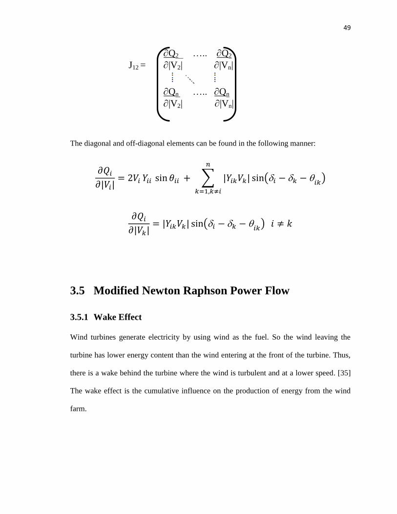
The diagonal and off-diagonal elements can be found in the following manner:
𝜕𝑃𝑖𝜕𝑖
= −𝑉𝑖 ∑ |𝑌𝑖𝑘𝑉𝑘|
𝑛
𝑘=1,𝑘≠𝑖
sin(𝑖 − 𝑘 − 𝑖𝑘)
𝜕𝑃𝑖𝜕𝑖
= |𝑉𝑖 𝑌𝑖𝑘𝑉𝑘| sin(𝑖 − 𝑘 − 𝑖𝑘) 𝑖 ≠ 𝑘
2. Formation of J12
This submatrix has a dimension of (n-1) x np. It is formed by differentiating the
active power with respect to the magnitude value of the voltage. Here, the magnitudes
values of the voltages are fixed and the derivate terms for the same are neglected.
P2 ….. P2
J12 = |V|2 |V|n
Pn ….. Pn
|V|2 |V|n
The diagonal and off-diagonal elements can be found in the following manner:
𝜕𝑃𝑖𝜕|𝑉𝑖|
= 2𝑉𝑖 𝑌𝑖𝑖 cos 𝜃𝑖𝑖 + ∑ |𝑌𝑖𝑘𝑉𝑘|
𝑛
𝑘=1,𝑘≠𝑖
cos(𝑖 − 𝑘 − 𝑖𝑘)
Page 58
48
𝜕𝑃𝑖𝜕|𝑉𝑘|
= |𝑌𝑖𝑘𝑉𝑘| cos(𝑖 − 𝑘 − 𝑖𝑘) 𝑖 ≠ 𝑘
3. Formation of J21
This (np) x (n-1) dimension submatrix is generated by finding the partial derivate
of the reactive power with respect to the voltage angle.
Q2 ….. Q2
J21 = δ2 δn
Qn ….. Qn
δn δn
The diagonal and off-diagonal elements can be found in the following manner:
𝜕𝑄𝑖𝜕𝛿𝑖
= 𝑉𝑖 ∑ |𝑌𝑖𝑘𝑉𝑘|
𝑛
𝑘=1,𝑘≠𝑖
cos(𝑖 − 𝑘 − 𝑖𝑘)
𝜕𝑄𝑖𝜕𝛿𝑖
= −|𝑉𝑖𝑌𝑖𝑘𝑉𝑘| cos(𝑖 − 𝑘 − 𝑖𝑘) 𝑖 ≠ 𝑘
4. Formation of J22
The matrix J22 is a (np) x (np) formed by the derivative values of the reactive power with
respect to the magnitude of the voltage value. It is given by:
Page 59
49
Q2 ….. Q2
J12 = |V2| |Vn|
Qn ….. Qn
|V2| |Vn|
The diagonal and off-diagonal elements can be found in the following manner:
𝜕𝑄𝑖𝜕|𝑉𝑖|
= 2𝑉𝑖 𝑌𝑖𝑖 sin 𝜃𝑖𝑖 + ∑ |𝑌𝑖𝑘𝑉𝑘|
𝑛
𝑘=1,𝑘≠𝑖
sin(𝑖 − 𝑘 − 𝑖𝑘)
𝜕𝑄𝑖𝜕|𝑉𝑘|
= |𝑌𝑖𝑘𝑉𝑘| sin(𝑖 − 𝑘 − 𝑖𝑘) 𝑖 ≠ 𝑘
3.5 Modified Newton Raphson Power Flow
3.5.1 Wake Effect
Wind turbines generate electricity by using wind as the fuel. So the wind leaving the
turbine has lower energy content than the wind entering at the front of the turbine. Thus,
there is a wake behind the turbine where the wind is turbulent and at a lower speed. [35]
The wake effect is the cumulative influence on the production of energy from the wind
farm.
Page 60
50
Figure 21 Wake Effect
In case of the model generated here, in order to calculate the wind speed for the turbines
in the second row, the following equation is used:
𝑈2 = 𝑈1𝐾
= 𝑈1 (1 − (1 − √1 − 𝑐𝑡) [𝐷
𝐷+2𝑘𝑋]2)
Where:
U1: Wind speed for the first turbine,
U2: Wind speed for the second turbine,
ct : turbine thrust coefficient,
D: Rotor diameter,
X: Axial distance between both wind turbines,
k: wake decay constant, calculated as,
Page 61
51
𝑘 = (𝐴ln (ℎ 𝑧0⁄⁄ )
Wherein:
A = 0.5
h: hub height
z0: roughness length
3.5.2 RX Bus Model with Wind Farm
The primary step involved in calculating the power flow for such an electrical
network is modeling of the farm. WT is considered to operate as a RX load with
equivalent impedance Z= R+jX, where R and X are Resistance and Reactance
respectively of the wind turbine. The inclusion of the wind turbine while excluding the
stator impedances modifies the NR power flow in the following manner:
Figure 22 Generator's Equivalent Circuit Discounting Stator Impedance
Page 62
52
Rs and Xs are disregarded and it is assumed that
(1 − 𝑠
𝑠) =
1
𝑠
Where, s is the slip of the wind turbine
|𝐼𝑟|2 =
|𝑉|2
(𝑅𝑟𝑠 + 1𝑠)2
+ 𝑋𝑟2
Mechanical power is computed by the formula:
𝑃𝑚𝑒𝑐ℎ = − |𝐼𝑟|2 𝑅𝑟𝑠
= −|𝑉|
2 𝑅𝑟 𝑠
(𝑠 + 1)2𝑅𝑟2 + 𝑠2𝑋𝑟
2
Organizing the above equation, the slip is derived as:
𝑠 = −(2𝑃𝑚𝑒𝑐ℎ𝑅𝑟 + |𝑉|
2 𝑅𝑟 ) ± √∆
2(𝑃𝑚𝑒𝑐ℎ𝑅𝑟2 + 𝑃𝑚𝑒𝑐ℎ𝑋𝑟
2)
Where,
∆ = (2𝑃𝑚𝑒𝑐ℎ𝑅𝑟2 + |𝑉|2 𝑅𝑟 )
2− 4𝑃𝑚𝑒𝑐ℎ𝑅𝑟
2(𝑃𝑚𝑒𝑐ℎ𝑅𝑟2 + 𝑃𝑚𝑒𝑐ℎ𝑋𝑟
2)
Page 63
53
The RX model is based on the steady state model with impedance Zwt.
𝑍𝑤𝑡 =𝑗𝑋𝑚 (𝑅𝑟
𝑠 + 1𝑠
+ 𝑗𝑋𝑐)
𝑅𝑟 𝑠 + 1𝑠
+ 𝑗(𝑋𝑚 + 𝑋𝑟)
= 𝑅1 + 𝑗𝑋1
Where, R1 and X1 are
𝑅1 = 𝑋𝑚
2𝑅𝑟 𝑠 + 1𝑠
(𝑅𝑟𝑠 + 1𝑠)2
+ (𝑋𝑚 + 𝑋𝑟)2
𝑋1 = 𝑋𝑚𝑋𝑟 (𝑋𝑚 + 𝑋𝑟) + 𝑋𝑚 (𝑅𝑟
𝑠 + 1𝑠)2
(𝑅𝑟𝑠 + 1𝑠)2
+ (𝑋𝑚 + 𝑋𝑟)2
The active power generated by the rotor windings and the input mechanical power can be
expressed as:
𝑃𝑔𝑒𝑛 = 𝐼𝑟2𝑅1
=(𝑆|𝑉|)2
𝑅𝑟𝑠 + 1𝑠
𝑋𝑚2
(𝑅𝑟𝑠 + 1𝑠)2
+ (𝑋𝑚 + 𝑋𝑟)2
𝑃𝑚𝑒𝑐ℎ = (𝑆|𝑉|)2
(1 − 𝑠) 𝑅𝑟 𝑠 + 1𝑠
𝑋𝑚2
𝑅𝑟𝑠 + 1𝑠
𝑋𝑚2
Page 64
54
The Jacobi matrix is then computed by the below equation
[𝐽] = 𝜕𝑃𝑚𝑒𝑐ℎ𝜕𝑠
𝜕𝑃𝑚𝑒𝑐ℎ𝜕𝑠
= 𝜕
𝜕𝑥{
(𝑆|𝑉|)2
𝑋𝑚(1 − 𝑠) 𝑅𝑟 𝑠 + 1𝑠
(𝑅𝑟𝑠 + 1𝑠)2
+ (𝑋𝑚 + 𝑋𝑟)2}
= 𝐴 {𝑅𝑟
2(1 − 4𝑠2 − 4𝑠3 − 𝑠4) − (𝑠2 + 𝑠4)(𝑋𝑚 + 𝑋𝑟)2
[𝑅𝑟2 + 𝑠2(𝑋𝑚 + 𝑋𝑟)
2]2 }
Where:
𝐴 = (𝑆
|𝑉|)2
𝑋𝑚2𝑅𝑟
𝑆 = √𝑃𝑔2 + 𝑄𝑐
2
𝑃𝑔 = −|𝑉|2
|𝑍𝑤𝑡| 𝑅𝑒(𝑍𝑤𝑡)
𝑄𝑐 = |𝑉|2
|𝑍𝑤𝑡| 𝐼𝑚(𝑍𝑤𝑡)
Page 65
55
With all the known values, now the active power extracted from the wind can be
determined in the following manner:
𝑃𝑤𝑖𝑛𝑑 = ½ 𝜌𝐴 𝑣𝑤𝑖𝑛𝑑3 𝐶𝑝
Where:
Ρ: Air density,
A: Swept area of blades,
vwind: Wind speed
Cp: Power coefficient, defined as
𝐶𝑝 = ½ (𝜆 – 5.6) 𝑒−0.17𝜆
Where:
λ: Tip speed ratio (TSR) of the wind turbine
R: length of the blade of the turbine
ωr: Rotor speed
𝜆 = 𝜔𝑟 𝑅
𝑣𝑤𝑖𝑛𝑑
= 𝜔𝑠 (1 − 𝑠) 𝑅
𝑣𝑤𝑖𝑛𝑑
Page 66
56
In general, due to the initially assumed slip value, the mechanical power and the
wind power are not equal to each other. After the first set of iterations of the power flow
calculations, if the difference between them is not zero, the new slip value is updated
continuously. The process stops when 𝛥𝑃𝑚 ≤ 휀.
𝛥𝑃𝑚 = 𝑃𝑤𝑖𝑛𝑑 − 𝑃𝑚𝑒𝑐ℎ
When the two powers are not equal, the next iteration begins. The result is updated in the
following manner:
𝑠𝑘+1 = 𝑠𝑘 + 𝛥𝑠
Where:
𝛥𝑠 = 𝐽−1 𝛥𝑃𝑚
Page 67
57
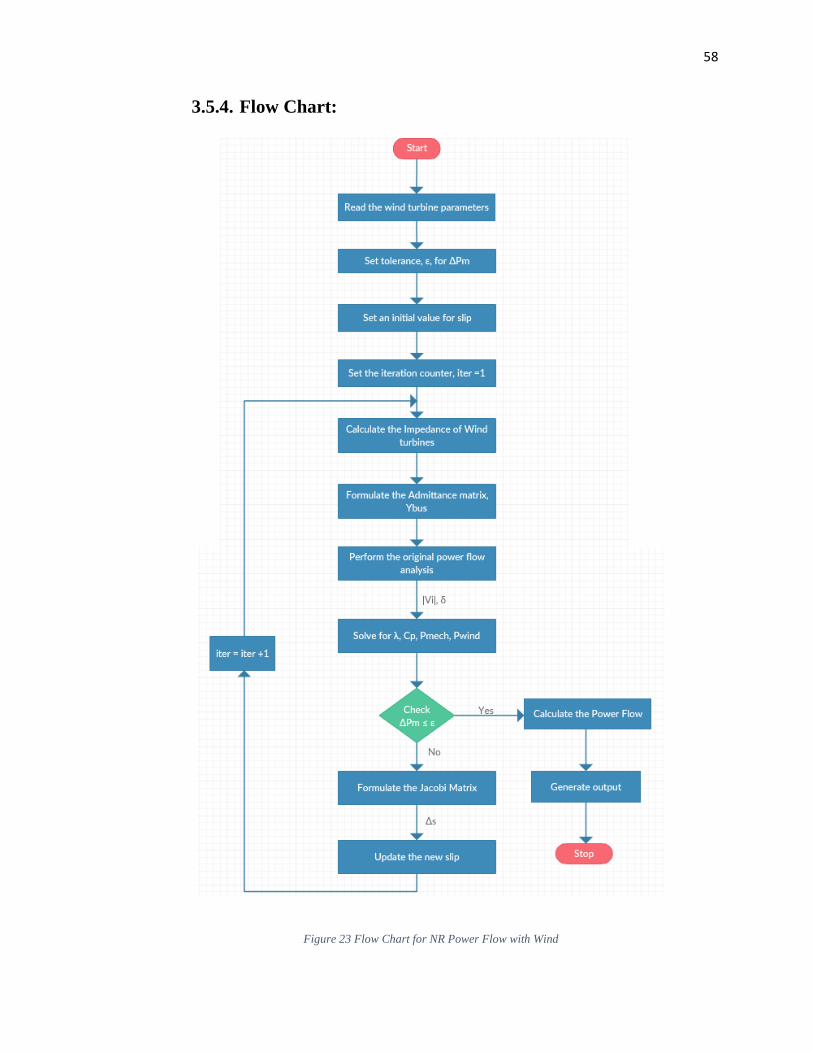
3.5.3 Algorithm
With the inclusion of Wind farm in the system, the Newton Raphson power flow
algorithm will be solved in the following manner:
1. A value of slip is assumed for the wind turbine which is equal to the rated slip. The
equivalent impedance, Zwt, is calculated using the proposed slip value.
2. Using the corresponding Zwt value, the admittance matrix is modified such that it
includes the admittance of the Wind turbines.
3. After the first iteration of the original power flow with the obtained voltages, the
input mechanical power is computed.
4. The wind power is calculated with the values of slip, TSR and power coefficient.
5. The difference between the two powers is found and the difference is checked against
the tolerance level. If the difference is not satisfied, the slip value is updated and all
the steps from Step 2 are solved. Otherwise, the iteration is stopped and the solution
is printed.
Page 68
58
3.5.4. Flow Chart:
Figure 23 Flow Chart for NR Power Flow with Wind
Page 69
59
3.6 Economic Dispatch
Any interconnected power system generally consists of three stages. The first
stage is production wherein the generators produce electrical energy. This is followed by
transmission of the power through transmission lines to meet the demand. The final stage
is the consumption of electricity by various loads. During each of these phases, some
amount of energy is lost to the environment. Thus, the main objective of a power system
is to supply power to the load continuously and as economically as possible. The process
of planning the power distribution and generation for each unit is done by optimizing the
power flow and the economic load dispatch.
The optimal power flow problem aims at optimizing the cost function, subject to
certain objectives, under provided capacity and network constraints. While, the network
constraints may include variables such as real and reactive power outputs, voltages
magnitudes, and phase angles at a number of buses, the objective may be the
minimization of generation cost and power losses while maximization of the lifetime of
the wind farm.
The economic load dispatch problem, on the other hand, allocates the generation
limit among the various generators, such that, the overall cost of generation is minimized
while meeting the constraints. Unlike optimal power flow, economic dispatch does not
consider power loss through the transmission lines, so the total power generated is real
and equal to the total load. The total cost of generation is analyzed as a quadratic
equation and includes the cost of labor, fuel cost, the maintenance and the supplies.
Page 70
60
Economic dispatch allows the allocation of output power in the power system
among all the available generators with the given constraints. This process of allocation
depends on various factors such as the security of the system, the operating cost and the
CO2 emissions which together are called as the cost factors.
3.6.1. Objective of Economic Dispatch Problem
The main objective of an economic dispatch problem is to minimize the operating
cost of real power generation. Both the constraints as well the objective function is non-
linear. The optimal combination of the power generators is detected such that the total
cost of generation is minimized while satisfying equality and inequality constraints. The
operating cost for conventional generators is a quadratic cost function which is
represented by
𝐶𝑖 (𝑝𝑖) = 𝑎𝑖2 𝑝𝑖2 + 𝑏𝑖𝑝𝑖 + 𝑐𝑖
Where:
pi: power from the ith
conventional generator
a, b, c: cost coefficients of the ith
generator
The variables a, b, and c values are dependent on the particular type of fuel used and the
input-output curve generated.
In case of wind power generators, there is a linear cost function involved. The
generation cost may not exist if the wind farms are owned by the power operators as the
power requires no fuel. But it may be considered as a maintenance cost, renewal cost or a
Page 71
61
payback cost. However, in a non-utility owned system, the generation through wind has a
price associated to it that may be based on special agreements.
This cost is represented as
𝐶𝑤,𝐼 (𝑤𝑖) = 𝑑𝑖𝑤𝑖
Where:
wi: the scheduled wind power from the ith
wind-powered generator
di: direct cost coefficient for the ith
wind generator
As we are aware, the wind speed is highly uncertain and unpredictable in nature,
so the power generated from wind is also highly ambiguous. From the figure below, the
variation of availability of wind energy over a certain period of time is observed. [36]
Figure 24 Wind Energy Availability over a Day
Page 72
62
There is surplus of wind wherein the wind power produced is more than the
scheduled wind power, wi, has a cost associated to it when the turbines are not owned by
the utility. So, if there is a surplus of unused wind power, the operator who owns the
turbine is paid a certain amount.
While, if there is a deficit of power, which occurs when available wind power is
less than scheduled, the difference in power has to be supplied or compensated by a
reserve power source such as standby generators, batteries or any such energy storing
systems.
Thus, the penalty cost applied for not utilizing all the available wind power at that
period of time is linearly related to the difference between the available wind power and
the actual wind power used. It is defined as:
𝐶𝑝,𝑤,𝑖 (𝑊𝑖,𝑎𝑣 – 𝑤𝑖) = 𝑘𝑝,𝑖 (𝑊𝑖,𝑎𝑣 – 𝑤𝑖)
= 𝑘𝑝,𝑖 ∫ (𝑤 – 𝑤𝑖) 𝑓𝑊(𝑤) 𝑑𝑤
𝑤𝑟,𝑖
𝑤𝑖
Where:
fW : Weibull distribution for wind speed after its conversion to wind power
kp,i: Penalty cost coefficient for the ith
wind generator due to the underestimation of
available wind
Page 73
63
Similarly, the reserve cost requirement is represented by the reserve power
wherein the scheduled wind power is not sufficient. So, the difference between the
scheduled and available wind power is integrated over the pdf value of the wind power. It
can be written as:
𝐶𝑟,𝑤,𝑖 (𝑤𝑖 − 𝑊𝑖,𝑎𝑣 ) = 𝑘𝑟,𝑖 (𝑤𝑖 − 𝑊𝑖,𝑎𝑣 )
= 𝑘𝑟,𝑖 ∫ (𝑤𝑖 − 𝑤) 𝑓𝑊(𝑤) 𝑑𝑤
𝑤𝑖
0
Where:
kr,i: Penalty cost coefficient for the ith
wind generator due to the overestimation of
available wind power
In order to simplify the model, the difference between the available and scheduled
wind power multiplied by the probability density function of the wind power output is
assumed to be linearly related to the reserve cost.
3.6.2. Constraints of the Economic Dispatch Problem
Each system operation should satisfy certain constraints to find a feasible solution
because of the operational limits in case of a practical system. These constraints include:
Constraints on generation capacity
The real power output in case of each generator is bound by upper and lower limits.
𝑝𝑖𝑚𝑖𝑛 ≤ 𝑝𝑖 ≤ 𝑝𝑖
𝑚𝑎𝑥
Page 74
64
0 ≤ 𝑤𝑖 ≤ 𝑤𝑟,𝑖
Where:
wr,I : the rated wind power from the ith
wind generator
Constraints on balancing the power values:
The total demand must be met by the total power from conventional and wind generators.
So,
∑𝑝𝑖
𝑀
𝑖=1
+ ∑𝑤𝑖
𝑁
𝑖=1
= 𝐿
Where:
M: Number of conventional power generators
N: Number of wind-powered generators
L: System load and losses
Constraints on operating the system:
𝑉𝑖𝑚𝑖𝑛 ≤ 𝑉𝑖 ≤ 𝑉𝑖
𝑚𝑎𝑥
𝑆𝑙𝑖𝑛𝑒𝑖 ≤ 𝑆𝑙𝑖𝑛𝑒𝑖𝑚𝑎𝑥
Where:
Vi: Magnitude of voltage at the ith
bus
Sline,I: Rating of the ith
transmission line
Page 75
65
In summation, the main objective of economic dispatch is to minimize the
operating cost from the conventional and wind- powered generators while including the
penalty cost from underestimation and overestimation of the wind power, while subject to
specific constraints.
The model for economic dispatch is defined in the following manner:
∑𝐶𝑖
𝑀
𝑖=1
(𝑝𝑖) + ∑𝐶𝑤,𝑖
𝑁
𝑖=1
(𝑤𝑖) +∑𝐶𝑝,𝑖
𝑁
𝑖=1
(𝑤𝑖) +∑𝐶𝑟,𝑖
𝑁
𝑖=1
(𝑤𝑖)
Subject to:
𝑝𝑖𝑚𝑖𝑛 ≤ 𝑝𝑖 ≤ 𝑝𝑖
𝑚𝑎𝑥
0 ≤ 𝑤𝑖 ≤ 𝑤𝑟,𝑖
∑𝑝𝑖
𝑀
𝑖=1
+ ∑𝑤𝑖
𝑁
𝑖=1
= 𝐿
𝑉𝑖𝑚𝑖𝑛 ≤ 𝑉𝑖 ≤ 𝑉𝑖
𝑚𝑎𝑥
𝑆𝑙𝑖𝑛𝑒𝑖 ≤ 𝑆𝑙𝑖𝑛𝑒𝑖𝑚𝑎𝑥
Page 76
66
3.7 Probability Analysis of Wind Power
In order to approach the economic dispatch with wind-powered generation
system, it is necessary to identify the wind speed characterization of the uncertainty
nature of wind through the principles of probability and the subsequent transformation to
wind power.
3.7.1 Wind Speed Characterization
The wind speeds, according to prior research [37], in a particular location, closely
follow and take the form of a Weibull distribution over time. The probability density
function (pdf) of the Weibull distribution is defined by the following equation:
𝐹𝑊(𝑤) = (𝑘
𝑐) (𝑤
𝑐)𝑘−1
𝑒−(𝑣𝑐)𝑘 0 < 𝑤 < ∞
Where:
W: wind speed random variable
w: wind speed
c: scale factor at a given location (units of wind speed)
k: shape factor at a given location (dimensionless)
The PDF value of Weibull distribution is:
𝐹𝑤(𝑤) = ∫ 𝑓(𝜏) 𝑑𝜏𝑤
0
Page 77
67
= 1 − 𝑒−(𝑤 𝑐⁄ )𝑘
CHAPTER 4:
IMPLEMENTATION AND RESULTS
4.1 Test Case: IEEE 14-Bus Test System
A standard IEEE 14 bus system is considered as a basic model for analysis. It
consists of 2 synchronous condensers at Buses 6, and 8 providing both active and reactive
powers. There are three synchronous condensers at Buses 3, 6 and 8. Automatic voltage
regulators (AVR) of type II are incorporated in each machine. The base generation of the
system is 392.0304MW and 204.2345MVar. Apart from that, there are 11 loads at Buses
2, 3, 4, 5, 6, 9, 10, 11, 12, 13, and 14. The general case is modeled in the following way
Figure 25 IEEE 14 Bus Single Line Diagram
Page 78
68
4.2 Wind Generator Placement
Consequently, the power grid model is modified into the smart grid which
incorporates wind energy into the bus. The model is represented as a single line diagram.
The simulation is generated using the Power System Analysis Toolbox (PSAT) in
MATLAB and is depicted in figure 19. Bus 6 is found to be the most suitable bus for
addition of the wind turbine due to its maximum strength stability and proven increased
penetration. [38] For simulation, GE’s 1.6MW wind turbines are used to construct the
wind farm. This wind farm is added at bus 6 in place of the synchronous condenser. It has
the following Parameters:
Parameters Value
Rated power, P (MW) 1.6
Rated voltage, V (kV) .69
Rated frequency, f (Hz) 50
Number of pole pairs, p 4
Rotor diameter, d (m) 100
Stator resistance, Rs (pu) 0.00706
Rotor resistance, Rr (pu) 0.005
Stator leakage inductance, Xs (pu) 0.171
Rotor leakage inductance, Xr (pu) 0.310
Magnetizing inductance, Xm (pu) 2.0
Gear ratio 1:91
Table 2 Wind Turbine Parameter
Page 79
69
Figure 26 Modified IEEE 14 bus with Wind Turbine [PSAT Model]
The wind farm is composed of two rows of wind turbines. It is ensured that they
are separated by a distance large enough to ensure that there is no interaction between the
two rows when the wind blows in a direction perpendicular to them. At the same time, it
Page 80
70
is made sure that they wind turbines are close enough to make the interaction among the
turbines important due to the presence of wake effect. The total wind power obtained
from the two rows of wind turbines is calculated by taking the wake effect into
consideration.
Furthermore, the line and bus data for the simulation are given in the tables
below.
LINE DATA:
Table 3 Line Data for Modified IEEE 14 Bus with Wind Farm
Page 81
71
BUS DATA:
Table 4 Bus Data for Modified IEEE 14 Bus with Wind Farm
Page 82
72
4.3 Results of the Modified Newton Raphson Power
Flow Algorithm
The results obtained in table 5, depict that the algorithm for the load flow analysis
converged after 4 iterations for a primary wind speed of 9m/s. The calculated value of the
slip for the turbine is -2.1321x 10⁻¹⁰
.
Solutions Value
No. of iterations 4
Tolerance, ε 1 x 10⁻⁴
Wind Turbine slip, s -2.1321x 10⁻¹⁰
Total active power generation (MW) 289.902
Total reactive power generation (MVar) 19.315
Total active load (MW) 259.000
Total reactive load (MVar) 73.500
Total active line loss (MW) 4.632
Total reactive line loss (MVar) 19.333
Table 5 Convergence characteristics and power system values
When compared to the values from actual power flow without wind, a remarkable
influence can be noticed on the bus voltage at bus 6, where the wind turbines are
connected.
Page 83
73
It is ensured that the calculated voltages across all buses, including bus 6 to which
the wind farm is connected, are within permitted limits. However, during exceptional
cases or faults, such as a short circuit occurring at the bus connected to the turbines, the
voltage values would be modified significantly. Apart from that, the rapid and dynamic
changes in wind speed would make the injected power in the network highly variable.
The rate of change and the intensity would in turn make the regulation of voltage
challenging which would directly impact the quality level of the electrical energy.
After the iterations for the electrical network are performed and the solution
converges, the load flow in each branch is found and represented in the model as shown
below. The sent and received active and reactive powers in each branch vary by a small
value. Every step of the iteration has been modeled below to represent the data at each
bus and the line losses. It is noticed that as the slip is varied, the solution converges and
the generation is increased while reducing the losses.
Page 84
74
ITERATION: 1
Table 6 Load Flow for Iteration1
Page 85
75
Table 7 Line Flow and Losses for Iteration1
Page 86
76
Figure 27 Power Flow Model for Iteration1
Page 87
77
ITERATION: 2
Table 8 Load Flow for Iteration 2
Page 88
78
Table 9 Line Flow and Losses for Iteration 2
Page 89
79
Figure 28 Power Flow Model for Iteration2
Page 90
80
ITERATION: 3
Table 10 Load Flow for Iteration 3
Page 91
81
Table 11 Line Flow and Losses for Iteration3
Page 92
82
Figure 29 Power Flow Model for Iteration 3
From the above results, we can draw conclusions that the total active and reactive
powers generated are 289.902 MW and 19.315 MVar. Out of this, the slack bus (bus 1)
was the major contributor towards the active power generation, providing 175.703MW.
The positive and negative signs in front of the power values designate if the power was
consumed by the bus or generated at that point.
Page 93
83
4.4 Economic Load Dispatch Model for the Modified
Test Case
In the preceding sections, the base IEEE 14 bus model was described and the
modified bus model incorporating the wind farm was developed. Weibull probability
distribution was used to model the wind speed and with the help of linear power
equations, from Chapter 3, the wind speed distributions were converted into wind power
distributions.
MATLAB was used to develop a program based on the economic dispatch model
with the modified case system to generate a tool to examine the effect of variations in
wind speeds and cost coefficients on the optimum solution of the ED problem. The
assumed wind farm parameters and generator data is specified below.
Table 13 Parameters of Wind Power Plant
Table 12 Generator Data for Modified IEEE 14 Bus Test System
BUS ai bi ci 𝑷𝒊𝒎𝒊𝒏 𝑷𝒊
𝒎𝒂𝒙
1 0.007 7 240 50 500
2 0.0095 10 200 20 200
3 0.009 8.5 220 20 300
6 0.009 11 200 20 150
8 0.008 10.5 220 20 200
Page 94
84
The economic dispatch is modeled to minimize the operating cost of the real
power generation in an electrical network. In order to achieve that various scenarios have
been taken into considerations such as, varying the shape and size parameters in Weibull
pdf, modifying the wind speed profile, etc. The best case is found with the least operating
cost that would satisfy the model. The different cases are as follows.
4.4.1. Effects of Wind Power Coefficients
The primary case would be the investigation of the effects of change in wind
speed profile on the output of the generators in the model. Initially, the penalty cost
coefficient would be zero for the prototype. This is the case where the wind farms are
owned by the power system operator. So, accessing a cost for overuse or no use is not
required.
The constants a, b, and c for the generators are taken from table 13. For the wind-
powered generator, the direct cost coefficient d =1.12 is assumed. Initially, no penalty
cost coefficient is assumed, a reserve cost coefficient of 1 is taken. This is followed by
cases wherein the wind farms are owned by the private entities, such that there is an over
estimation and under estimation cost involved. These situations are not always ideal in
terms of threats caused to the stability and security of the system.
The critical wind speed parameters for the turbines are provided in table 12. The
scale factor for the Weibull pdf is varied from 5 to 25. While the shape factor is kept
constant at k=2.
Page 95
85
Based on the Weibull distribution, the scale factor, c has a proportional impact on
the wind speeds. As the c factor increases, the probability of obtaining a greater
proportion of wind speed also increases.
4.4.1.1. Effect of Reserve Cost Coefficient
Firstly, assuming that the wind farms are owned by utility so the penalty cost of
the additionally available wind power over the scheduled wind power, kp = 0. As the
scale factor of the Weibull pdf grows, the reserve cost decreases.
Figure 30 Effect of Reserve Cost Coefficient on the Output
Figure 23 verifies the above statement. The graph is plotted by taking the various
values of reserve cost coefficients. When the value of c which is the scale factor
increases, there is a greater amount of wind energy, which means there is more available
wind power from the generators. However, at a higher reserve cost, the wind at a higher
speed becomes less attractive and the output of the turbine falls to a lower rate. So, the
Page 96
86
reduction in reserve cost, in turn increases the output of wind powered generators. Hence,
increasing the reserve cost coefficient requires the operator to be more conservative with
the scheduling of energy as a greater price would have to be paid for overestimating the
amount of scheduled wind power in a given time frame under certain restrictions.
4.4.1.2. Effect of Penalty Cost Coefficient
The effect of the penalty cost coefficient for underestimation is modeled next. In
this scenario, the reserve cost coefficient is set to 0 in order to isolate the changes of
the penalty cost coefficients.
Figure 31 Effect of Penalty Cost Coefficient
The effect of penalty cost on the scheduled output is explained in figure 24. With
the increase in the penalty cost coefficient, kp more wind power would have to be used
Page 97
87
for the model. This is because with increase in kp, the operator is encouraged to take more
risk, thereby increasing the scheduled wind power limit. This in turn means that as the
wind farm has the ability to meet the load demand under no reserve cost, the other
conventional generators would be kept at their minimal levels.
Therefore, the previous two sections provide a stronger understanding of the
trends involved with the inclusion of wind energy into the electrical network. So, an
increase in the reserve cost coefficient would decrease the scheduled amount of wind
power, while an increase in the penalty cost coefficient would increase the scheduled
amount of wind power.
Page 98
88
CHAPTER 5:
Conclusion and Future Scope
5.1. Conclusion
The tremendous potential of wind energy, along with its environment-friendly
distinction and its increasing competitiveness in the energy market, has made it one of the
most popular fuels for power generation in the modern era. It is quickly becoming one the
preeminent technologies to provide a viable and sustainable source to the world’s
development, but is still shrouded in misunderstandings due to lack of research. This
makes it imperative to conduct in-depth studies and research in order to understand and
comprehend the wind power generation and develop modern ways to integrate the wind
farms into existing electrical networks.
With the increase of penetration of wind power, the process of integration of wind
farms to power grids is getting trickier as it involves understanding the significant
influences on the already existent host system. Moreover, in order to become competitive
in the liberalized market, precise prediction of the generation levels for each moment of
the day is essential. Thus, there is a need for more reliable and accurate models for
performing the power simulation analysis that could account for the variability and
inconsistency of wind availability.
Page 99
89
The preliminary step of the research has been focused on modeling a load flow
system. Proper analysis is required for finding a method for distributing the power within
an electrical grid when a Wind Energy Conversion System has been included. For this
purpose, the wind farm has been modeled as an RX load bus and the already existing
Newton-Raphson Power Flow method has been modified to incorporate the new bus
system such that it would reflect the real, accurate, and steady output of the generators. In
this paper, we consider a wind farm with 10 turbines used to replace a synchronous
condenser at bus 6 in the IEEE 14 bus system. The changes in the power generation are
observed and vetted against an existing model consisting of conventional generators. The
simulation results validate that the model is effective for practical use and has the
capability to converge in lesser time. The proposed model and the technique involved in
computing the system can be further utilized for more complex distributions.
Apart from analyzing the power distribution, it is essential to further comprehend
the irregular nature of wind speed to generate an algorithm to modulate the power
allocation. The uncertainty of wind is modeled by the Weibull probability density
function. To the already existing economic dispatch model, two more factors accounting
for the over- and under-estimations of available wind power is added. The reserve and the
penalty cost factors play a vital role while scheduling the amount of wind power. So, if
the reserve cost coefficient is increased, the scheduled amount of power from the wind
farms will be reduced as over-estimation of the wind power, while it increases the load on
other generators. This increases the need for other conventional generators to produce
more energy to satisfy the load requirements. Conversely, if the penalty cost coefficient is
increased, it means that the wind farms are not being utilized to their full potential. This
Page 100
90
provides the operator an incentive to take more risk and increase the scheduled amount of
wind power. In both cases, the efficiency of the system is reduced. Thus, these
incremental costs, when compared to quadratic costs of the conventional units, could
provide a simplified economic model that would incorporate both thermal and wind
power.
Analytical arguments have been presented to demonstrate that the proposed
algorithm is capable of achieving the minimum cost allocation under certain constraints
over time. This developed model can be further used as a fundamental design in the
future for building more cost-efficient environmental-friendly systems.
5.2. Future Scope
5.2.1. Algorithm Optimization
The basic algorithm for economic dispatch with wind farm integration described
in this research can be refined and extended in numerous ways. Using the provided model
and constraints, the optimum minimal solution can be found. There are several
optimization techniques available which can be applied to the economic dispatch
problem. Such improvements can use basic calculus or can include modern stochastic
searching solutions, such as the direct search method, particle swarm optimization,
Lagrangian relaxation, genetic algorithm and simulated annealing. These optimization
techniques provide a precise oversimplified model of the system with the help of
contemporary mathematical properties. Using optimization tools, we can generate a
system such that the load allocation is more accurate and none of the generators are
loaded above the safe point.
Page 101
91
5.2.2. Incorporation into Smart Grids
The research has been motivated by the needs to satisfy the future grid networks by
providing a system wherein the generators and the load respond intelligently. This would
enable a real-time system and maximize the efficiency for better energy utilization. It is
imperative to extend the load flow and the cost optimization problem into a distributed
approach.
5.2.3. Storage System
The economic dispatch model with wind energy has two more factors which
account for the over-estimation or under-estimation of wind power. At the time of under-
estimation, such as during the nighttime or when more wind is generated, the excess of
energy can be stored for future use. The inclusion of a storage system can be an effective
option as it would allow for a larger penetration of such renewable energy resources. This
would warrant that the efficiency is not reduced and the excess energy can be stored in a
battery or in some other form. One such example could be the running of the Robert
Moses Niagara Power Plant at night by using the excess energy generated by the wind
farms rather than depending on generators.
Page 102
92
Bibliography
[1] R. Register, EcoCities: Rebuilding Cities in Balance with Nature, New Society
Publishers, 2006.
[2] G. E. I. D. a. C. Organization, "Smart Grid," Geidco, 2016. [Online]. Available:
http://www.geidco.org/html/qqnycoen/col2015100801/column_2015100801_1.html.
[3] P. M. Chi Seng Leun, "How electricity consumption affects social and economic
development".
[4] S. Sceptic, "Enerconics: The Relationship between Energy and GDP," October
2013. [Online]. Available: http://scottishsceptic.co.uk/2013/10/18/enerconics-the-
relationship-between-energy-and-gdp/.
[5] K. Klaiman, "Total U.S. electricity sales projected to grow slowly as electricity
intensity declines," 2016. [Online]. Available:
https://www.eia.gov/todayinenergy/detail.php?id=26672.
[6] Statista, "Energy's share of business sector Gross Domestic Product, by country,"
2017. [Online]. Available: https://www.statista.com/statistics/217556/percentage-of-
gdp-from-energy-in-selected-countries/.
[7] "Energy Information Administration," 2016. [Online]. Available:
https://www.eia.gov/tools/faqs/faq.php?id=427&t=3.
[8] J. Leonard, "Wind tops list as most promising renewable energy source," 2009.
[Online]. Available: http://www.futurity.org/wind-tops-list-as-best-renewable-
energy/.
[9] A. W. A. Energy, "U.S. number one in the world in wind energy production," 29
February 2016. [Online]. Available:
https://www.awea.org/MediaCenter/pressrelease.aspx?ItemNumber=8463.
[10] S. Ashok and R. Banerjee, "An optimization mode for industrial load management,"
in IEEE Transactions on Power Systems, 2001.
[11] A. a. A. F. Ipakchi, "Grid of Future," in IEEE power & energy magazine, 2009.
[12] P. Street, "Pecan Street," [Online]. Available: http://www.pecanstreet.org/what-is-
pecan-street-inc/.
[13] S. C. Collaborative, Smart Grid Economic and Environmental Benefits: A Review
and Synthesis of Research on Smart Grid Benefits and Costs, Smart Grid Consumer
Collaborative, 2013.
[14] C. Weare, The California Electricity Crisis: Causes and Policy Options, PUBLIC
Page 103
93
POLICY INSTITUTE OF CALIFORNIA, 2003.
[15] E. A. Committee, "Smart Grid: Enabler of the New Energy Economy," 2008.
[16] A. Drachmann, ""Heron's Windmill"," Centaurus, 1961.
[17] M. Sathyajith, "Wind Energy: Fundamentals, Resource Analysis and Economics,"
2006.
[18] Wikipedia, "History_of_wind_power," [Online]. Available:
https://en.wikipedia.org/wiki/History_of_wind_power.
[19] Wikipedia, "James Blyth," [Online]. Available:
https://en.wikipedia.org/wiki/James_Blyth_(engineer).
[20] GEWC, "Market Forecast 2012-2016," [Online]. Available:
http://www.gwec.net/global-figures/market-forecast-2012-2016/ .
[21] GWEC, "Wind in Numbers," [Online]. Available: http://www.gwec.net/global-
figures/wind-in-numbers/ .
[22] S. Wind, "The challenges of wind turbine maintenance in China," 2017. [Online].
Available: http://windfarmmanagement.skf.com/a-tall-order/.
[23] A. W. E. A. (AWEA), " Wind Vision: A New Era for Wind Power in the United
States," Wind Vision, [Online]. Available: https://www.awea.org/doe-wind-vision.
[24] F. Exploring, "Wind Turbines and the Energy in Wind," [Online]. Available:
http://www.ftexploring.com/energy/wind-enrgy.html.
[25] W. P. Program, "Power curve," Wind Power Program, [Online]. Available:
https://www.wind-power-program.com/popups/powercurve.htm.
[26] J. Z. a. S. Xu, "Jianzhong Zhang and Shuai Xu (2015). Application of Fuzzy Logic
Control for Grid-Connected Wind Energy Conversion System, Fuzzy Logic - Tool
for Getting Accurate Solutions, Prof. Elmer Dadios (Ed.), InTech, DOI:
10.5772/59923. Available from: https://www.," in Application of Fuzzy Logic
Control for Grid-Connected Wind Energy Conversion System, 2015.
[27] IGET, "What are the Basic Wind Turbine Configurations?," [Online]. Available:
https://www.igetcol.it/turbine.htm.
[28] Turbinesinfo, "Horizontal Axis Wind Turbines – HAWT," Turbines Info, 05 July
2011. [Online]. Available: http://www.turbinesinfo.com/horizontal-axis-wind-
turbines-hawt/.
[29] E. W. E. Association, "The Economics of Wind Energy," 2009.
[30] G. J. a. R. Piwko, "The Value of Wind Power Forecasting," in 91st American
Page 104
94
Meteorological Society Annual Meeting, the Second Conference on Weather,
Climate, and the New Energy Economy, Washington, DC, 2011.
[31] M. Ragheb,
"http://mragheb.com/NPRE%20475%20Wind%20Power%20Systems/Economics%
20of%20Wind%20Energy.pdf," 2017.
[32] W. E. Foundation, "Wind Energy Economics," Wind Energy Foundation, [Online].
Available: http://windenergyfoundation.org/about-wind-energy/economics/.
[33] B.Stott, "Review of Load –Flow Calculation Methods," 1974.
[34] T. T. P. a. V. L. Nguyen, "RX Model-Based Newton Raphson Load Flow for
Distribution Power System Considering Wind Farm with Asynchronous
Generators," GMSARN International Journa, vol. 10, pp. 11-18, 2016.
[35] D. W. I. Association, "Wake Effect," 2003.
[36] 1957CHEV, "Why Intermittent Wind Power Increases CO2 Emissions in the
Electricity Sector," 7 September 2014. [Online]. Available:
https://mothersagainstwindturbines.com/2014/09/07/wind-turbines-increase-the-
amount-of-co2-being-produced-to-make-electricity/.
[37] M. R. Patel, Wind and Solar Power Systems, Boca Raton, 2005.
[38] Q. Yang, J.-H. Zhang, Z. Wu, W. Li and J. Yang, "Analysis on Stability of
Integration of Wind Farms into Power Systems," in Power and Energy Engineering
Conference, 2009.